LarKC The Large Knowledge Collider a platform for large scale integrated reasoning and Web-search FP7 – 215535 D4.3.1 Strategies and Design for Interleaving Reasoning and Selection of Axioms Coordinator: [Zhisheng Huang (VUA)] With contributions from: [Zhisheng Huang (VUA), Yi Zeng (WICI), Stefan Schlobach (VUA), Annette den Teije (VUA), Frank van Harmelen (VUA), Yang Wang (WICI), Ning Zhong (WICI) Quality Assessor: [Gulay Unel (STI)] Quality Controller: [Frank van Harmelen (VUA)] Document Identifier: LarKC/2008/D4.3.1/V1.0 Class Deliverable: LarKC EU-IST-2008-215535 Version: version 1.0.0 Date: September 29, 2009 State: final Distribution: public
Transcript
LarKCThe Large Knowledge Collider
a platform for large scale integrated reasoning and Web-search
FP7 – 215535
D4.3.1Strategies and Design forInterleaving Reasoning and
Selection of Axioms
Coordinator: [Zhisheng Huang (VUA)]With contributions from: [Zhisheng Huang (VUA), Yi Zeng(WICI), Stefan Schlobach (VUA), Annette den Teije (VUA),
Frank van Harmelen (VUA), Yang Wang (WICI), NingZhong (WICI)
Quality Assessor: [Gulay Unel (STI)]Quality Controller: [Frank van Harmelen (VUA)]
Document Identifier: LarKC/2008/D4.3.1/V1.0Class Deliverable: LarKC EU-IST-2008-215535Version: version 1.0.0Date: September 29, 2009State: finalDistribution: public
FP7 – 215535
Deliverable 4.3.1
Executive Summary
In this document, we discuss the main features of Web scale reasoning and develop aframework of interleaving reasoning and selection. We examine the framework of inter-leaving reasoning and selection with the LarKC platform. The framework is exploredfurther from the following three perspectives: i) Query-based selection. We proposevarious query-based strategies of interleaving selection and reasoning with respect tothe LarKC data sets; ii) Granularity-based selection. We investigate the Web scalereasoning from the perspective of granular reasoning, and develop several strategiesof Web scale reasoning with granularity; and iii) Language-based selection. We pro-pose an approach of classification with anythime behaviours based on approximatereasoning and report the results of the experiments with several realistic ontologies.
2 of 64
FP7 – 215535
Deliverable 4.3.1
Document Information
IST ProjectNumber
FP7 – 215535 Acronym LarKC
Full Title The Large Knowledge Collider: a platform for large scale integratedreasoning and Web-search
In this document, we discuss the main features of Web scale reasoningand develop a framework of interleaving reasoning and selection. Weexamine the framework of interleaving reasoning and selection with theLarKC platform. The framework is explored further from the followingthree perspectives: i) Query-based selection. We propose various query-based strategies of interleaving selection and reasoning with respect tothe LarKC data sets; ii) Granularity-based selection. We investigate theWeb scale reasoning from the perspective of granular reasoning, and de-velop several strategies of Web scale reasoning with granularity; and iii)Language-based selection. We propose an approach of classification withanythime behaviours based on approximate reasoning and report the re-sults of the experiments with several realistic ontologies.
Keywords Reasoning, Selection, Semantic Web, Web scale reasoning
3 of 64
FP7 – 215535
Deliverable 4.3.1
Project Consortium Information
Participant’s name Partner ContactSemantic Technology Institute Innsbruck,Universitaet Innsbruck
Prof. Dr. Dieter FenselSemantic Technology Institute (STI),Universitaet Innsbruck,Innsbruck, AustriaEmail: [email protected]
AstraZeneca AB Bosse AnderssonAstraZenecaLund, SwedenEmail: [email protected]
5.1 Comparison of predicted and actual completeness value. . . . . . . . . . 345.2 Normalized edge degree distribution in the SwetoDBLP RDF dataset. . 375.3 Coauthor number distribution in the SwetoDBLP dataset. . . . . . . . 385.4 log-log diagram of Figure 5.3. . . . . . . . . . . . . . . . . . . . . . . . 385.5 A zoomed in version of Figure 5.3. . . . . . . . . . . . . . . . . . . . . 385.6 A zoomed in version of coauthor distribution for “Artificial Intelligence”. 385.7 Publication number distribution in the SwetoDBLP dataset. . . . . . . 385.8 log-log diagram of Figure 5.7. . . . . . . . . . . . . . . . . . . . . . . . 38
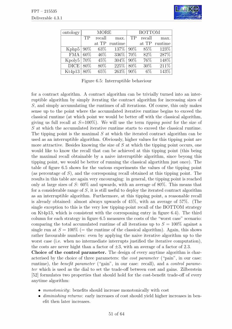
6.1 anytime performance profile from examples 1 and 2 . . . . . . . . . . . 456.2 Some properties of the ontologies used in our experiments . . . . . . . . 476.3 Results for the MORE strategy on the DICE ontology . . . . . . . . . . 486.4 Summary of success and failure of the different strategies. . . . . . . . . 506.5 Interruptible behaviour . . . . . . . . . . . . . . . . . . . . . . . . . . . 516.6 . . . . . . . . . . . . . . . . . . . . . . . . . . . . . . . . . . . . . . . . 52
7 of 64
FP7 – 215535
Deliverable 4.3.1
List of Acronyms
Acronym Description
DL Description LogicsOWL Web Ontology LanguagePION The System of Processing Inconsistent OntologiesRDF Resource Description FrameworkRDFS Resource Description Framework SchemaSPARQL SPARQL Protocol And RDF Query Language
8 of 64
FP7 – 215535
Deliverable 4.3.1
1. Introduction
Web scale reasoning has become a crucial issue for practical applications of the Seman-tic Web, because of the extremely large scale data on the Web. Web scale semanticdata have the following main features:
• Infiniteness. There are extremely large amount of semantic data on the Web.Till June 2009, Linked Data have reached the scale of above four billion triples.More linked data are expected to grow rapidly in coming few years. Therefore,Web scale data can be considered to be infinitely scalable.
• Dynamics. Web scale data are in flux. They are growing extremely rapidly, sothat it is hard to know what the clear border of data is.
• Inconsistency. Re-using and combining multiple ontologies on the Web isbound to lead to inconsistencies between the combined vocabularies. Even manyof the ontologies that are in use today turn out to be inconsistent once some oftheir implicit knowledge is made explicit. Therefore, infinitely scaled Web datatend to be semantically inconsistent. Moreover, consistency checking of Webscale data is impossible because of the infinite scale.
Because of those features of Web scale data, many traditional notions of reasoning arenot valid any more. Essence of the LarKC project is to go beyond tranditional notionsof absolute correctness and completeness in reasoning. We are looking for retrievalmethods that provide useful responses at a feasible cost of information acquisition andprocessing. Therefore, generic inference methods need to be extended to non-standardapproaches.
In this document, we will explore an approach of Web scale reasoning, in whichvarious strategies of interleaving reasoning and selection are developed, so that thereasoning processing can focus on limited part of data to improve the scalability ofWeb scale reasoning. This approach is inspired by our previous work on reasoningwith inconsistent ontologies[19]. However, in this document we will develop a generalframework of interleaving reasoning and selection, so that it can deal with not onlyreasoning with inconsistent ontologies, but also generic Web scale data.
Collins and Quillian observe that knowledge is stored as a system of propositionsorganized hierarchically in memory [11], in problem solving, human can focus on ap-propriate levels to avoid redundant information. Minsky remarks that in order to avoidthe failure of understanding knowledge in one way, knowledge should be representedfrom different viewpoints [28]. As an emerging field of study, Granular Computingextracts the commonality of human and machine intelligence and emphasizes on mul-tilevel and Multiperspective organization of granular structures [47].
In this document, we will develop various strategies under the notion of granu-lar reasoning to solve the problems for Web scale reasoning. Inspired by CognitiveScience, Artificial Intelligence and Granular Computing, we bring the strategies ofmultilevel, multiperspective, starting point to Web scale reasoning. With user in-volvement, switching among different levels and perspectives during the process ofreasoning is the basic philosophy of granular reasoning. From the multilevel point ofview, in order to meet different levels of user needs, we can provide reasoning resultswith variable completeness and variable specificity. From the multiperspective pointof view, reasoning can be based on different perspectives of the knowledge source.
9 of 64
FP7 – 215535
Deliverable 4.3.1
Reasoning based on starting point utilizes the user background and provides mostimportant reasoning results to users. These strategies is aimed at satisfying a widevariety of user needs and removing the scalability barriers.
Anytime algorithms are attractive for Web scale reasoning, because they allowa trade-off between the cost of the algorithm and the quality of the results. Suchanytime algorithms have been developed for many AI reasoning tasks, such as plan-ning, diagnosis and search. However, until now no anytime methods exist yet forsubsumption-based classification in Description Logics. This is important among theother problems because classification is essential to Semantic Web applications, whichrequire reasoning over large or complex ontologies.
In this document, we will present an algorithm for classification with anytimebehaviour based on approximate subsumption. We give formal definitions for approx-imate subsumption, and show soundness and monotonicity. We develop an algorithmand heuristics to obtain anytime behaviour for classification reasoning. This anytimebehaviour can be realised with classical DL reasoners. We study the computationalbehaviour of the algorithm on a set of realistic ontologies. Our experiments showattractive performance profiles. The most interesting finding is that anytime classifi-cation works best where it is most needed: on ontologies where classical subsumptionis hardest to compute.
This document is organized as follows: In Chapter 2 we discuss the main features ofWeb scale reasoning and develop a framework of interleaving reasoning and selection.In Chapter 3 we explore the framework from the perspective of query-based selection.In Chapter 4 we examine the framework of interleaving reasoning and query-basedselection with the LarKC platform and propose several strategies of interleaving selec-tion and reasoning with respect to the LarKC data sets. In Chapter 5 we investigatethe Web scale reasoning from the perspective of granular reasoning, and develop sev-eral strategies of Web scale reasoning with granularity. In Chapter 6 we propose anapproach of classification with anythime behaviours based on approximate reasoningand report the results of the experiments with several realistic ontologies. In Chapter7 we discuss the future work and conclude the document.
10 of 64
FP7 – 215535
Deliverable 4.3.1
2. A Framework of Interleaving Reasoning and Selection
2.1 Web Scale Reasoning
Web scale reasoning is reasoning with Web scale semantic data. As we discussed before,The main features of Web scale semantic data are: i)Infiniteness. There are extremelylarge amount of semantic data on the Web. They can be considered to be infinitelyscalable. ii) Dynamics. Web data are in flux. There is no a clear border of data,and iii) Inconsistency. It is most likely that so large amount of data are semanticallyinconsistent. However, consistency checking of Web scale data is impossible.
Those features of Web scale data force us to re-examine the traditional notion ofreasoning. The classical notion of reasoning is to consider the consequence relationbetween a knowledge base (i.e. a formula set Σ) and a conclusion (i.e., a formula φ),which is defined as follows:
Σ |= φ iff for any model M of Σ, M is a model of φ.
For Web scale reasoning, Knowledge base Σ can be considered as an infinite formulaset. However, when the cardinality |Σ| of the knowledge base Σ becomes infinite and Σis inconsistent, many notions of logic and reasoning in classical logics, including manyexisting description logics, which are considered to be standard logics for ontologyreasoning and the Semantic web, are not valid any more.
It is worthy to mention that classical logics do not limit the cardinality of theirknowledge bases to be finite, because the compactness theorem in classical logics wouldhelp them to deal with the infiniteness.
The Compactness theorem states that:
(CT) a (possibly infinite) set of first-order formulas has a model, iff every finite subsetof it has a model,
Or conversely:
(CT’) a (possibly infinite) set of formulas doesn’t have a model if there exists itsfinite subset that doesn’t have a model.
That means that given an infinite set of formulas Σ and a formula φ, if we canfind a finite subset Σ′ ⊆ Σ such that Σ′ ∪ {¬φ} is unsatisfiable (namely, there existsno model to make the formula set holds), it is sufficiently to conclude that φ is aconclusion of the infinite Σ. In other words, the compactness theorem means thatin the formalisms based on FOL we can positively answer the problems of the formΣ |= φ, by showing that Σ ∪ {¬φ} |= contradiction. Thus, we have chances to show(even if Σ is infinite) if we are able to identify a finite subset of Σ (call it Σ′ ) suchthat Σ′ ∪ {¬φ} |= contradiction.
However, we would like to point out that the compactness theorem would not helpfor Web scale reasoning because of the following reason.
For Web scale data, Knowledge base Σ may be inconsistent. Now, consider theproblem to answer the form Σ |= φ where Σ is inconsistent. When Σ is inconsistent,a finite subset of Σ (call it Σ′) such that Σ′ ∪ {¬φ} |= contradiction would not besufficient to lead to a conclusion that Σ |= φ, because there might exist another subsetof Σ (call it Σ′′) such that Σ′′ ∪ {φ} |= contradiction.
11 of 64
FP7 – 215535
Deliverable 4.3.1
If we re-examine the classical notions of the complexity in the setting of Web scalereasoning, many those of the notions would also become meaningless. Just take theexample of the complexity of finding the answer problems of the form Σ |= φ. Considera polynomial complexity with respect to the complexity of knowledge base Σ, say, alinear complexity O(|Σ|). When Σ becomes infinite, a linear complexity would becomeintractable.
2.2 Framework of Web Scale Reasoning by Interleaving Reason-ing and Selection
A way out to solve the infiniteness and inconsistency problems of Web scale reasoningis to introduce a selection procedure so that our reasoning processing can focus on alimited (but meaningful) part of the infinite data. That is the motivation for developingthe framework of Web scale reasoning by interleaving reasoning and selection.
Therefore, the proceddure of Web scale reasoning by interleaving reasoning andselection consists of the following selection-reasoning-decicison-loop:
Algorithm 2.1: Selection-Reasoning-Loop
repeatSelection: Select a (consistent) subset Σ′ ⊆ ΣReasoning: Reasoning with Σ′ |= φ to get answersDecision: Deciding whether or not to stop the processing
until Answers are returned.Namely, the framework depends on the following crucial processes: i) How can
we select a subset of a knowledge base and check the consistency of selected data, ii)How can we reason with selected data, iii) how can we make the decision whether ornot the processing should be stop. That usually depends on the problem how we canevaluate the answer obtained from the process ii), Our framework is inspired by ourprevious work in reasoning with inconsistent ontologies[19]. Since Web scale data maybe inconsistent, we can apply the same framework to deal with the problem of Webscale reasoning.
In the following, we will explore the framework further from the following threeperspectives: i) Query-based selection. We propose various query-based strategies ofinterleaving selection and reasoning; ii) Granularity-based selection. We investigatethe Web scale reasoning from the perspective of granular reasoning, and develop severalselection strategies of Web scale reasoning with granularity; and iii) Language-basedselection. We propose an approach of classification with anythime behaviours based onsub-language selection and report the results of the experiments with several realisticontologies.
12 of 64
FP7 – 215535
Deliverable 4.3.1
3. Query-based Selection Strategies
3.1 Selection Functions
Selection functions play the main role in the framework of interleaving reasoning andquery-based selection. A system of interleaving reasoning and query-based selectionuses a selection function to determine which subsets of a knowledge base should beconsidered in its reasoning process. This general framework is independent of theparticular choice of selection function. The selection function can either be based on asyntactic approach, like Chopra, Parikh, and Wassermann’s syntactic relevance [8] andthose in PION[19], or based on semantic relevance like for example in computationallinguistics as in Wordnet [7] or based on semantic relevance which is measure by theco-occurrence of concepts in search engines like Google[22].
In our framework, selection functions are designed to query-specific, which is differ-ent from the traditional approach in belief revision and nonmonotoic reasoning, whichassumes that there exists a general preference ordering on formulas for selection. Givena knowledge base Σ and a query φ, a selection function s is one which returns a sub-set of Σ at the step k > 0. Let L be the ontology language, which is denoted as aformula set. A selection function s is a mapping s : P(L)× L×N → P(L) such thats(Σ, φ, k) ⊆ Σ.
A selection function s is called monotonic if the subsets it selects monotonicallyincrease or decrease, i.e., s(Σ, φ, k) ⊆ s(Σ, φ, k + 1), or vice versa. For monotonicallyincreasing selection functions, the initial set is either an emptyset, i.e., s(Σ, φ, 0) = ∅,or a fixed set Σ0. For monotonically decreasing selection functions, usually the initialset s(Σ, φ, 0) = Σ. The decreasing selection functions will reduce some formulas fromthe inconsistent set step by step until they find a maximally consistent set.
Traditional reasoning methods cannot be used to handle knowledge bases withlarge scale. Hence, selecting and reasoning on subsets of Σ may be appropriate as anapproximation approach with monotonically increasing selection functions. Web scalereasoning on a knowledge base Σ can use different selection strategies to achieve thisgoal. Generally, they all follow an iterative procedure which consists of the followingprocessing loop, based on the selection-reasoning-decision loop discussed above:i) select part of the knowledge base, i.e., find a subset Σ′
i of Σ where i is a positveinteger, i.e., i ∈ I+;ii) apply the standard reasoning to check if Σ′
i |= φ;iii) decide whether or not to stop the reasoning procedure or continue the reasoningwith gradually increased selected subgraph of the knowledge graph (Hence, Σ′
1 ⊆ Σ′2 ⊆
... ⊆ Σ).Monotonically increasing selection functions have the advantage that they do not
have to return all subsets for consideration at the same time. If a query can beanswered after considering some consistent subset of the knowledge graph KG forsome value of k, then other subsets (for higher values of k) don’t have to be consideredany more, because they will not change the answer of the reasoner. In the following,we use Σ |= φ to denote that φ is a consequence of Σ in the standard reasoning1, anduse Σ |≈ φ to denote that φ is a consequence of Σ in the nonstandard reasoning.
1Namely, for any model M of Σ, M |= φ.
13 of 64
FP7 – 215535
Deliverable 4.3.1
Figure 3.1: Linear Extension Strategy.
3.2 Strategies
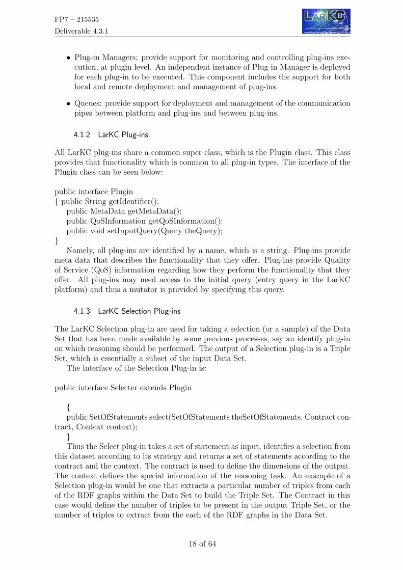
A linear extension strategy is carried out as shown in Figure 3.1. Given a queryΣ |≈ φ, the initial consistent subset Σ′ is set. Then the selection function is calledto return a consistent subset Σ′′, which extends Σ′, i.e., Σ′ ⊂ Σ′′ ⊆ Σ for the linearextension strategy. If the selection function cannot find a consistent superset of Σ′,the inconsistency reasoner returns the answer ‘undetermined’ (i.e., unknown) to thequery. If the set Σ′′ exists, a classical reasoner is used to check if Σ′′ |= φ holds. Ifthe answer is ‘yes’, the reasoner returns the ’accepted’ answer Σ |≈ φ. If the answer is‘no’, the reasoner further checks the negation of the query Σ′′ |= ¬φ. If the answer is‘yes’, the reasoner returns the ’rejected’ answer Σ |≈ ¬φ, otherwise the current resultis undetermined, and the whole process is repeated by calling the selection functionfor the next consistent subset of Σ which extends Σ′′.
It is clear that the linear extension strategy may result in too many ‘undetermined’answers to queries when the selection function picks the wrong sequence of monotoni-cally increasing subsets. It would therefore be useful to measure the successfulness of(linear) extension strategies. Notice, that this depends on the choice of the monotonicselection function.
In general, one should use an extension strategy that is not over-determined (i.e.,the selected set is inconsistent) and not undetermined. For the linear extension strat-egy, we can prove that a reasoner using a linear extension strategy may be undeter-mined, always sound, and always meaningful[20]. A reasoner using a linear extensionstrategy is useful to create meaningful and sound answers to queries. The advantagesof the linear strategy is that the reasoner can always focus on the current working setΣ′2. The reasoner doesn’t need to keep track of the extension chain. The disadvantageof the linear strategy is that it may lead to an inconsistency reasoner that is undeter-mined. There exists other strategies which can improve the linear extension approach,
2Alternatively it is called the selected set.
14 of 64
FP7 – 215535
Deliverable 4.3.1
for example, by backtracking and heuristics evaluation. We will discuss how it can beachieved in the over-determined processing in Section Over-determined Processing.
3.3 Relevance based Selection Functions
[8] proposes a syntactic relevance to measure the relationship between two formulasin belief sets, so that the relevance can be used to guide the belief revision based onSchaerf and Cadoli’s method of approximate reasoning[34]. Given a formula set Σ,two atoms p, q are directly relevant, denoted by R(p, q,Σ) iff there is a formula α ∈ Σsuch that p, q appear in α. A pair of atoms p and q are k-relevant with respect to Σiff there exist p1, p2, . . . , pk ∈ L such that: (a) p, p1 are directly relevant; (b) pi, pi+1
are directly relevant, i = 1, . . . , k − 1; and (c) pk, q are directly relevant (i.e., directlyrelevant is k-relevant for k = 0).
The notions of relevance above are based on propositional logics. However, ontologylanguages are usually written in some fragment of the first order logic. We extend theideas of relevance to ontology language. The Direct relevance between two formulasare defined as a binary relation on formulas, namely R ⊆ L × L. Given a directrelevance relation R, we can extend it to a relation R+ on a formula and a formulaset, i.e., R+ ⊆ L× P(L) as follows:
〈φ,Σ〉 ∈ R+ iff ∃ψ ∈ Σ such that 〈φ, ψ〉 ∈ R.
Namely, a formula φ is relevant to a knowledge base Σ iff there exists a formulaφ′ ∈ Σ such that φ and φ′ are directly relevant. We can similarly specialize the notionof k-relevance. Two formulas φ, φ′ are k-relevant with respect to a formula Σ iff thereexist formulas φ0, . . . φk ∈ Σ such that φ and φ0, φ0 and φ1, . . ., and φk and φ′ aredirectly relevant. A formula φ is k-relevant to a set Σ iff there exists a formula φ′ ∈ Σsuch that φ and φ′ are k-relevant with respect to Σ.
We can use a relevance relation to define a selection function s to extend the query‘Σ |≈ φ?’ as follows: We start with the query formula φ as a starting point for theselection based on syntactic relevance. Namely, we define:
s(Σ, φ, 0) = ∅.
Then the selection function selects the formulas ψ ∈ Σ which are directly relevant toφ as a working set (i.e. k = 1) to see whether or not they are sufficient to give ananswer to the query. Namely, we define:
s(Σ, φ, 1) = {ψ ∈ Σ | φ and ψ are directly relevant}.
If the reasoning process can obtain an answer to the query, it stops. Otherwise theselection function increases the relevance degree by 1, thereby adding more formulasthat are relevant to the current working set. Namely, we have:
s(Σ, φ, k) = {ψ ∈ Σ | ψ is directly relevant to s(Σ, φ, k − 1)},
for k > 1. This leads to a ”fan out” behavior of the selection function: the first selectionis the set of all formulae that are directly relevant to the query; then all formulae areselected that are directly relevant to that set, etc. This intuition is formalized in this:
15 of 64
FP7 – 215535
Deliverable 4.3.1
The relevance-based selection function s is monotonically increasing. We observe thatIf k ≥ 1, then
s(Σ, φ, k) = {φ|φ is (k-1)-relevant to Σ}
The relevance-based selection functions defined above usually grows up to an incon-sistent set rapidly. That may lead to too many undetermined answers. In order toimprove it, we can require that the selection function returns a consistent subset Σ′′
at the step k when s(Σ, φ, k) is inconsistent such that s(Σ, φ, k− 1) ⊂ Σ′′ ⊂ s(Σ, φ, k).It is actually a kind of backtracking strategies which are used to reduce the num-ber of undetermined answers to improve the linear extension strategy. We call theprocedure an over-determined processing(ODP) of the selection function. Note thatthe over-determined processing does not need to exhaust the powerset of the sets(Σ, φ, k)− s(Σ, φ, k−1), because of the fact that if a consistent set S cannot prove ordisprove a query, then nor can any subset of S. Therefore, one approach of ODP is toreturn just a maximally consistent subset. Let n be |Σ| and k be n− |S|, i.e., the car-dinality difference between the ontology Σ and its maximal consistent subset S (notethat k is usually very small), and let C be the complexity of the consistency checking.The complexity of the over-determined processing is polynomial to the complexity ofthe consistency checking. Note that ODP introduces a degree of non-determinism:selecting different maximal consistent subsets of s(Σ, φ, k) may yield different answersto the query Σ |≈ φ. The simplest example of this is Σ = {φ,¬φ}.
16 of 64
FP7 – 215535
Deliverable 4.3.1
4. Interleaving Reasoning and Selection in the LarKC Platform
4.1 LarKC Platform
4.1.1 LarKC Architecture
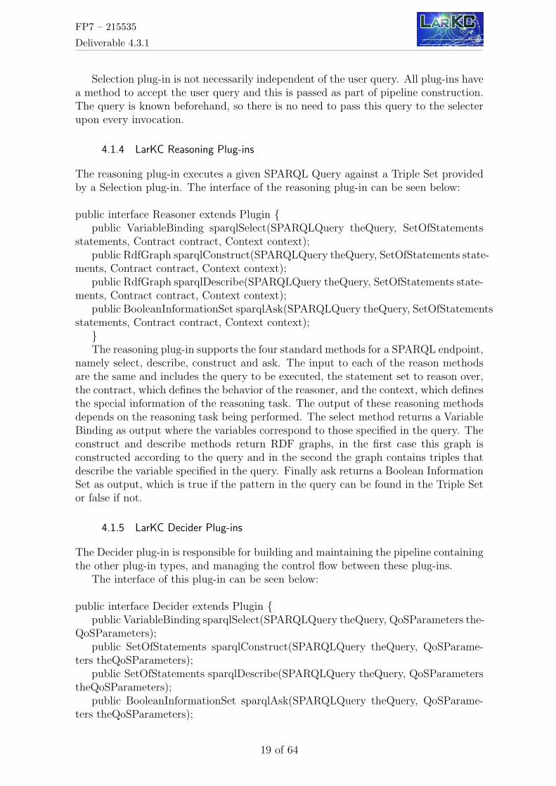
In this document, we consider the LarKC architecture which has been proposed in[43]. Figure 4.1 shows a detailed view of the LarKC Platform architecture.
The LarKC platform has been designed in a way so that it is as lightweight aspossible, but must provide all necessary features to support both users and plug-ins.For this purpose, the following components are distinguished as part of the LarKCplatform:
• Plug-in API: it defines interfaces for required behaviour from plug-in and there-fore provides support for interoperability between platform and plug-ins andbetween plug-ins.
• Data Layer API: the Data Layer provides support for data access and manage-ment via its API.
• Plug-in Registry: it contains all necessary features for plug-in registration anddiscovery
• Pipeline Support System: it provides support for plug-in instantiation, throughthe deployment of plug-in managers, and for monitoring and controlling plug-inexecution at pipeline level.
Figure 4.1: The LarKC Platform Architecture
17 of 64
FP7 – 215535
Deliverable 4.3.1
• Plug-in Managers: provide support for monitoring and controlling plug-ins exe-cution, at plugin level. An independent instance of Plug-in Manager is deployedfor each plug-in to be executed. This component includes the support for bothlocal and remote deployment and management of plug-ins.
• Queues: provide support for deployment and management of the communicationpipes between platform and plug-ins and between plug-ins.
4.1.2 LarKC Plug-ins
All LarKC plug-ins share a common super class, which is the Plugin class. This classprovides that functionality which is common to all plug-in types. The interface of thePlugin class can be seen below:
public interface Plugin{ public String getIdentifier();
public MetaData getMetaData();public QoSInformation getQoSInformation();public void setInputQuery(Query theQuery);
}Namely, all plug-ins are identified by a name, which is a string. Plug-ins provide
meta data that describes the functionality that they offer. Plug-ins provide Qualityof Service (QoS) information regarding how they perform the functionality that theyoffer. All plug-ins may need access to the initial query (entry query in the LarKCplatform) and thus a mutator is provided by specifying this query.
4.1.3 LarKC Selection Plug-ins
The LarKC Selection plug-in are used for taking a selection (or a sample) of the DataSet that has been made available by some previous processes, say an identify plug-inon which reasoning should be performed. The output of a Selection plug-in is a TripleSet, which is essentially a subset of the input Data Set.
tract, Context context);}Thus the Select plug-in takes a set of statement as input, identifies a selection from
this dataset according to its strategy and returns a set of statements according to thecontract and the context. The contract is used to define the dimensions of the output.The context defines the special information of the reasoning task. An example of aSelection plug-in would be one that extracts a particular number of triples from eachof the RDF graphs within the Data Set to build the Triple Set. The Contract in thiscase would define the number of triples to be present in the output Triple Set, or thenumber of triples to extract from the each of the RDF graphs in the Data Set.
18 of 64
FP7 – 215535
Deliverable 4.3.1
Selection plug-in is not necessarily independent of the user query. All plug-ins havea method to accept the user query and this is passed as part of pipeline construction.The query is known beforehand, so there is no need to pass this query to the selecterupon every invocation.
4.1.4 LarKC Reasoning Plug-ins
The reasoning plug-in executes a given SPARQL Query against a Triple Set providedby a Selection plug-in. The interface of the reasoning plug-in can be seen below:
public interface Reasoner extends Plugin {public VariableBinding sparqlSelect(SPARQLQuery theQuery, SetOfStatements
statements, Contract contract, Context context);}The reasoning plug-in supports the four standard methods for a SPARQL endpoint,
namely select, describe, construct and ask. The input to each of the reason methodsare the same and includes the query to be executed, the statement set to reason over,the contract, which defines the behavior of the reasoner, and the context, which definesthe special information of the reasoning task. The output of these reasoning methodsdepends on the reasoning task being performed. The select method returns a VariableBinding as output where the variables correspond to those specified in the query. Theconstruct and describe methods return RDF graphs, in the first case this graph isconstructed according to the query and in the second the graph contains triples thatdescribe the variable specified in the query. Finally ask returns a Boolean InformationSet as output, which is true if the pattern in the query can be found in the Triple Setor false if not.
4.1.5 LarKC Decider Plug-ins
The Decider plug-in is responsible for building and maintaining the pipeline containingthe other plug-in types, and managing the control flow between these plug-ins.
}The interface of the Decider plug-in is very similar to that of the reasoning plug-in.
The major difference is that actual data to reason over is not explicitly specified, asthe Identify plug-in is responsible for finding the data within the pipeline.
4.2 Interleaving Reasoning and Selection
In the following, we examine a framework of interleaving reasoning and selection inthe setting of the LarKC platform. We will propose several selection functions whichwhich are based on the LarKC data model, namely, in which a knowledge base isconsidered to be triple sets.
In the LarKC platform, ontology data are represented as a SetofStatements. Namely,they are a set of RDF statements. We can consider a RDF statement as a triple. Thus,conceptually, ontology data can be considered as a set of triples. Alternatively, it iscalled a triple set. A triple t has the form 〈s, p, o〉 where s is called a subject, p iscalled a predicate, and o is called an object of the triple.
For OWL ontology data, we usually use the popular DL reasoners such as Racer,FACT++, KAON2, and Pellet to obtain the standard DL reasoner support if OWLontology data is consistent and can be handled by those DL reasoners. All of thosepopular Dl reasoners provide the DIG interface. Thus, those popular DL reasonerscan serve as an external reasoner which can be called within the LarKC platform viaits DIG interface reasoner plugin. Furthermore, OWL APIs provide OWL-DL/OWL2reasoning interface, which is considered as a new generation and updated DIG inter-face. Thus, in the LarKC platform, we will use the OWL APIs reasoner plug-in forreasoning with OWL ontology data. In the following, we will use |= to denote thestandard DL reasoning.
In the LarKC platform, a query of a reasoner is represented as a SPARQL query,like sparqlAsk and sparqlSelect, which have been discussed in the previous section. TheSPARQL query language is designed for querying with RDF data originally. Thus, itis too powerful for a DL-based reasoner for reasoning with OWL ontology data. Thus,we will consider only the limited part of the SPARQL language, which is called asSPARQL-DL, i.e., the part of the SPARQL which corresponds with DL expressionssemantically. SPARQL-DL can be considered as a special case of conjunctive queriesfor DL, which provide a facility for databaselike querying with DL data. In the follow-ing, we will use a formula φ to denote a SPARQL-DL query. Semantically, a formulaφ corresponds to be a set of triples which is implied by the formula. Namely,
[[φ]] = {t : φ |= t}
A SparqlAsk query corresponds with a query formula φ in which there are no freevariables. A SparqlSelect query corresponds with a query formula φ in which thereare some free variables. For a triple set Σ and a query φ, we use Σ |= φ to denote thatΣ |= t for all t ∈ [[φ]].
Various selection functions can be defined in the LarKC platform. In the following,we will propose several selection functions for the processing of interleaving reasoningand selection.
20 of 64
FP7 – 215535
Deliverable 4.3.1
4.3 Syntactic Relevance based Selection Functions
Syntactic relevance means that the relevance is measured with respect to symbolic ap-pearrance of two triple sets without considering the semantics of the symbols. However,we should ignore the predicates of triples when two trilples are examined with respectto their relevance, because many predicates such as ”rdf:type” and ”rdfs:subClassOf”appear frequently in a RDF/RDFS data set, which suggests nothing on the relevanceof two triples. Thus, we can define a syntactic relevance relation Syn on two triplesas follows.
For any triple t1 = 〈s1, p1, o1〉 and any triple t2 = 〈s2, p2, o2〉,
〈t1, t2〉 ∈ Syn iff s1 = s2 or s1 = o2 s2 = o1 or o1 = o2.
Thus, we can extend this relevance measure to the relevance measure between atriple and a triple set Σ as discussed in the previous chapter. Namely, a triple t issaid to be relevant with a triple set Σ if there exists a triple t′ ∈ Σ such as t and t′
are relevant (with respect to the relation Syn). Furthermore, we can define a relevantsubset of a triple set Σ with respect to a relevance relation Syn and a triple set Σ′,written Syn(Σ,Σ′) as follows:
Syn(Σ,Σ′) = {t ∈ Σ : t is relevant with Σ′ with respect to the relevance relationSyn.}
Now, we can define a selection function s with respect to a relevance relation Synas follows:
(i) s(Σ, φ, 0) = ∅;(ii)s(Σ, φ, 1) = Syn(Σ, [[φ]]);(iii) s(Σ, φ, k) = Syn(Σ, s(Σ, φ, k − 1)), for k > 1.
Furthermore, we can define a syntactic relevance relation SynC which considers onlythe relevance with concepts as follows:
For any triple t1 = 〈s1, p1, o1〉 and any triple t2 = 〈s2, p2, o2〉,
〈t1, t2〉 ∈ SynC iff 〈t1, t2〉 ∈ Syn and((p1 =”rdfs:subClassOf” and o1 6=”owl:Thing” and s1 6=”owl:Nothing”) or(p2 =”rdfs:subClassOf” and o2 6=”owl:Thing” and s2 6=”owl:Nothing”)).
In the concept relevance measure above, we consider the triples which state thesubClassOf relation and ignore their relevance of the trivial subClassOf relation viathe top concept and the bottom concept.
4.4 Semantic Relevance based Selection Functions
The syntactic relevance-based selection functions prefer shorter paths to longer pathsin the reasoning. It requires knowledge engineers should carefully design ontologies toavoid unbalanced reasoning path. Naturally we will consider semantic relevance basedselection functions as alternatives of syntactic relevance based selection functions. In[22] we propose a semantic relevance based section function that is developed basedon Google distances. Namely, we want to take advantage of the vast knowledge on
21 of 64
FP7 – 215535
Deliverable 4.3.1
the web by using Google based relevance measure, by which we can obtain light-weight semantics for selection functions. The basic assumption here is that: morefrequently two concepts appear in the same web page, more semantically relevantthey are, because most of web pages are meaningful texts. Therefore, informationprovided by a search engine can be used for the measurement of semantic relevanceamong concepts. We select Google as the targeted search engine, because it is themost popular search engine nowaday. The second reason why we select Google is thatGoogle distances are well studied in [10, 9].
In [10, 9], Google Distances are used to measure the co-occurrence of two keywordsover the Web. Normalized Google Distance (NGD) is introduced to measure semanticdistance between two concepts by the following definition:
NGD(x, y) =max{logf(x), logf(y)} − logf(x, y)
logM −min{logf(x), logf(y)}
wheref(x) is the number of Google hits for the search term x,f(y) is the number of Google hits for the search term y,f(x, y) is the number of Google hits for the tuple of search terms x and y, and,M is the number of web pages indexed by Google.NGD(x, y) can be understood intuitively as a measure for the symmetric condi-
tional probability of co-occurrence of the search terms x and y.NGD(x, y) takes a real number between 0 and 1. NGD(x, x) = 0 means that
any search item is always the closest to itself. NGD(x, y) is defined for two searchitems x and y, which measures the semantic dissimilarity, alternatively called semanticdistance, between them.
The semantic relevance is considered as a reverse relation of the semantic dissimi-larity. Namely, more semantically relevant two concepts are, smaller distance betweenthem. Mathematically this relation can be formalized by the following equation if thesimilarity measurement and the distance measurement take a real number between 0and 1.
Similarity(x, y) = 1−Distance(x, y).
In the following we use the terminologies semantic dissimilarity and semantic dis-tance interchangeably. To use NGD for reasoning with inconsistent ontologies, weextend this dissimilarity measure on two triples in terms of the dissimilarity measureon the distances between two concepts/roles/individuals from the two triples. More-over, in the following we consider only concept names C(t) as the symbol set of a triplet to simplify the formal definitions. However, note that the definitions can be easilygeneralized into ones in which the symbol sets contain roles and individuals. We useSD(t1, t2) to denote the semantic distance between two triples. We expect semanticdistances between two formulas SD(t1, t2) satisfying the following intuitive properties:
• (i) (Range) The semantic distances are real numbers between 0 and 1. Namely,0 ≤ SD(t1, t2) ≤ 1 for any t1 and t2.
• (ii) (Reflexivity) Any triple is always semantically closest to itself. Namely,SD(t, t) = 0 for any t.
22 of 64
FP7 – 215535
Deliverable 4.3.1
• (iii) (Symmetry) The semantic distances between two triples are symmetric.Namely, SD(t1, t2) = SD(t2, t1) for any t1 and t2.
• (iv) (Remoteness) If all symbols in a triple is semantically most-dissimilarfrom any symbol of another triple, then these two triples are totally semantic-dissimilar. Namely, if NGD(Ci, Cj) = 1 for all Ci ∈ C(t1) and Cj ∈ C(t2), thenSD(t1, t2) = 1.
• (v) (Intermediary) If there are some shared symbols which appear in bothtriples and some symbols are semantically dissimilar between two triples, thenthe semantic distance between two triples are neither the closest, nor are themost dissimilar. Namely, if C(t1) ∩ C(t2) 6= ∅ and C(t1) 6= C(t2), then 0 <SD(t1, t2) < 1.
However, note that the semantic distance does not always satisfy the triangle Inequality
SD(t1, t2) + SD(t2, t3) ≥ SD(t1, t3),
a basic property of distances in a metric topology. [25] provides a counter-example ofthe Triangle Inequality in semantic similarity measure.
Simple ways to define the semantic distance between two triples is to take the mini-mal or the maximal or the average NGD values between two concepts/roles/individualswhich appear in two triples as follows:
where |C(t)| means the cardinality of C(t). However, it is easy to see that SDmin
and SDmax do not satisfy the property (v)Intermediary, and SDave do not satisfy theproperties (ii) Reflexivity and (iv) Remoteness.
In the following, we propose a semantic distance which is measured by the ratio ofthe distance sum of the difference between two formulas to the total distance sum ofthe symbols between two triples.
Definition 1 (Semantic Distance between two triples)
SD(t1, t2) = sum{NGD(Ci, Cj)|Ci, Cj ∈ (C(t1)/C(t2))∪(C(t2)/C(t1))}/(|C(t1)| ∗ |C(t2)|)
It is easy to prove that the following proposition holds:
Proposition 4.4.1 The semantic distance SD(φ, ψ) satisfies the properties (i)Range,(ii)Reflexivity, (iii)Symmetry, (iv)Remoteness, and (v)Intermediary.
23 of 64
FP7 – 215535
Deliverable 4.3.1
Using the semantic distance defined above, we can define a relevance relation forselection functions. Naturally, an easy way to define a direct relevance relation betweentwo triples in an ontology Σ is to define them as the semantically closest triples, i.e.,there exist no other triples in the ontology that is semantically more close, like this,
Based on the semantic relevance above, we can define the selection functions likethose defined in the previous section.
Using semantic distances, we propose a specific approach to deal with subsumptionqueries which have the form like C1 v D where C1 is a concept. In this new approach,C1 is considered as a center concept of the query, and the newly defined selectionfunction will track along the concept hierarchy in an ontology and always add theclosest formulas (to C1) which have not yet been selected, into the selected set asfollows:
s(Σ, C1 v D, 0) = ∅.
Then the selection function selects the formulas φ ∈ Σ which is the closest to C1 asa working set (i.e. k = 1) to see whether or not they are sufficient to give an answerto the query. Namely, we define1
If the reasoning process can obtain an answer to the query, it stops. Otherwisethe selection function selects the formulas that are closest to the current working set.Namely, we have:
s(Σ, C1 v D, k) = {t ∈ Σ | ¬∃t′ ∈ Σ(SD(t′, C1) <SD(t, C1) ∧ ψ 6∈ s(Σ, C1 v D,k − 1))} ∪ s(Σ, C1 v D, k − 1)
for k > 1.
4.5 Strategies
4.5.1 Variant Strategies of Interleaving Reasoning and Selection
Various strategies can be developed for interleaving reasoning and selection of axioms.In Chapter 5, we will intestigate the processing of interleaving reasoning and selectionvia a relevance measure with respect to the connections among nodes in triples. Thatwould provide an approach of granular reasoning in which varous granularity of webscale data can be selected for reasoning to improve the scalability. In Chapter 6, wewill propose a different strategies for interleaving reasoning and selection of axioms,by selecting a sub-language of ontology data, namely, by focusing on axioms in whichsome pre-selected concepts appear.
1It is easy to see the definition about SD(t1, t2) is easily extended into a definition about SD(t1, C),where t1, t2 are triples, and C is a concept.
24 of 64
FP7 – 215535
Deliverable 4.3.1
4.5.2 Strategies for Over-determined Processing
For inconsistent ontology data, reasoning extension procedure usually grows up toan inconsistent set rapidly. That may lead to too many undetermined answers. Inorder to improve it, over-determined processing (ODP) is introduced, by which werequire that the selection function returns a consistent subset Σ′′ at the step k whens(Σ, φ, k) is inconsistent such that s(Σ, φ, k − 1) ⊂ Σ′′ ⊂ s(Σ, φ, k). It is actually akind of backtracking strategies used to reduce the number of undetermined answersto improve the extension strategy. An easy solution to the over-determined processingis to return the first maximal consistent subset (FMC) of s(Σ, φ, k), based on certainsearch procedure. Query answers which are obtained by this procedure are still sound,because they are supported by a consistent subset of the ontology. However, it doesnot always provide intuitive answers because it depends on the search procedure ofmaximal consistent subset in over-determined processing.
One of the improvements for the over-determined processing is to use the semanticrelevance information. For example, we can prune semantically less relevant pathsto obtain a maximal consistent set. Namely, In the over-determined processing, thereasoning processing will remove the most dissimilar formulas from the set s(Σ, φ, k)−s(Σ, φ, k−1) first, until it can find a maximal consistent set such that the query φ canbe proved or disproved.
25 of 64
FP7 – 215535
Deliverable 4.3.1
5. Unifying Search and Reasoning from the Viewpoint of Gran-ularity
5.1 Introduction
The assumption of traditional reasoning methods do not fit very well when facingWeb scale data. One of the major problems is that acquiring all the relevant data isvery hard when the data goes to Web scale. Hence, unifying reasoning and search isproposed [12]. Under this approach, the search will help to gradually select a smallset of data (namely, a subset of the original dataset), and provide the searched resultsfor reasoning. If the users are not satisfied with the reasoning results based on the subdataset, the search process will help to select other parts or larger sub dataset preparedfor producing better reasoning results [12]. One detailed problem is that how to searchfor a good or more relevant subset of data and do reasoning on it. In addition, thesame strategy may not meet the diversity of user needs since their backgrounds andexpectations may differ a lot. In this chapter, we aim at solving this problem.
Granular computing, a field of study that aims at extracting the commonality ofhuman and machine intelligence from the viewpoint of granularity [46, 47], emphasizesthat human can always focus on appropriate levels of granularity and views, ignoringirrelevant information in order to achieve effective problem solving [47, 49]. Thisprocess contains two major steps, namely, the search of relevant data and problemsolving based on searched data. As a concrete approach for problem solving based onWeb scale data, the unification of search and reasoning also contains these two steps,namely, the search of relevant facts, and reasoning based on rules and searched facts.A granule is a set of elements that are drawn together by their equality, similarities,indistinguishability from some aspects (e.g. parameter values) [45]. Granules can begrouped into multiple levels to form a hierarchical granular structure, and the hierarchycan also be built from multiple perspectives [47]. Following the above inspirations, theweb of data can be grouped together as granules in different levels or under differentviews for searching of subsets and meeting various user needs. From the perspective ofgranularity, we provide various strategies for unifying user driven search and reasoningunder time constraints. From the multilevel point of view, in order to meet user needsin different levels, unifying search and reasoning with multilevel completeness andmultilevel specificity are proposed. Furthermore, from the multiperspective point ofview, the unifying process can be investigated based on different perspectives of theknowledge source. We also propose unifying search and reasoning with a startingpoint, which is inspired by the basic level advantage from cognitive psychology [32],to achieve diversity and scalability.
Section 5.2 introduces some basic notions related to this study. Section 5.3 give avery preliminary discussion on the search and reasoning process on a knowledge graph.The rest of this chapter focuses on introducing various strategies for unifying searchand reasoning from the viewpoint of granularity: Section 5.4 discusses the startingpoint strategy. Section 5.5 introduces the multilevel completeness strategy. Section 5.6introduces unifying strategy with multilevel specificity. Section 5.7 investigates on themultiperspective strategy. In Section 5.8, for each strategy introduced in this chapter,we provide some preliminary experimental results based on a semantic Web datasetSwetoDBLP, an RDF version of the DBLP dataset [3]. Section 5.9 discusses some
26 of 64
FP7 – 215535
Deliverable 4.3.1
related work. Finally, Section 7 makes concluding remarks by highlighting majorcontributions of this chapter.
5.2 Basic Notions
In this section, we introduce some basic notions for unifying selection and reasoningfrom the viewpoint of granularity, namely, knowledge graph, granule, level, perspective,which are fundamental thoughts that this study is built upon.
5.2.1 Knowledge Graph
We consider knowledge graphs as a general data model for Web data/knowledge (e.g.,RDF/RDFS data and OWL ontologies). Thus, in this chapter, granular reasoning isbased on graph representation of knowledge.
Definition 2 (Knowledge Graph) A knowledge graph (KG) is defined as:
KG = 〈N,E, T 〉, (5.1)
where N is a set of nodes, E is a set of edges, and T is a triple set of N × E ×N .1
In a knowledge graph, the edges are with directions, and the nodes can be understoodas classes in RDF/RDFS modeling. The relationship of two nodes in a knowledgegraph is represented as a triple t = 〈s, p, o〉. The subject (s) and object (o) are nodesfrom N , and the predicate (p) is from the set of edges (namely p ∈ E). T is a set oftriple sets (t ∈ T ). 2
Definition 3 (Node Degree) For a node n in the knowledge graph KG = 〈N,E, T 〉,its degree degree(n) is measured by:
The normalized degree(n) or normalized degree(e) can give a relative evaluationon the importance of the node or the edge in the KG.
1The definition of the knowledge graph can be extended to be with weighted edges. Namely, aweighted knowledge graph WKG = 〈N,E, T, R〉 where R : T → R is a mapping which assigns atriple t ∈ T a real number r ∈ R.
2A knowledge graph is said to be a first order one if its node set and its edge set are disjoint (i.e.,N ∩ E = ∅). If a knowledge graph G is a second order one, then an edge can be a node.
27 of 64
FP7 – 215535
Deliverable 4.3.1
5.2.2 Granule
In the context of the KG, a granule is a set of nodes that are grouped together byequality, similarity, indistinguishability, etc [14, 47]. A granule can be a singleton, i.e.,{n}. When a granular is a singleton, we can use a node n to denote a granule.
We define a general binary relation “contains” to represent the hierarchical relationamong granules3. We assume that this relation satisfy the following rational postulates:
In a knowledge graph, there might be various types of edges, if we consider creating aseries of subgraphs by a subset of the edge type, several subgraphs reflecting differentcharacteristics of the knowledge graph can be acquired.
Definition 6 (Perspective) In a knowledge graph KG, a perspective P is a subsetof edges (i.e., P ⊆ E).
A perspective is a viewpoint to investigate the KG. It can be a singleton (namely,P = {e}) or a set of predicates. Different perspectives reflect various characteristicsof the graph. The set of all perspectives P ⊆ E collectively describe a graph frommultiple viewpoints. Under a specified perspective, a subgraph of KG is generated,the node degree of this subgraph may reflect a unique characteristic of the originalKG.
Definition 7 (Node Degree under a Perspective) The Node Degree under a per-spective is defined as:
degree(n, P ) = degreein(n, P ) + degreeout(n, P ),degreein(n, P ) = |{〈s, p, n〉 : 〈s, p, n〉 ∈ T and p ∈ P}|,degreeout(n, P ) = |{〈n, p, o〉 : 〈s, p, n〉 ∈ T and p ∈ P}|,
(5.5)
where degreein(n, P ) and degreeout(n, P ) denote the indegree and outdegree for thenode n under the perspective P respectively.
Proposition 5.2.1 (Formal Properties of Node Degree under a Perspective)For a knowledge graph KG = 〈N,E, T 〉, the following properties hold:(1) Monotonicity: P ′ ⊆ P ′′ ⇒ degree(n, P ′) ≤ degree(n, P ′′),
(2) Triviality: P ′ = E ⇒ degree(n, P ′) = degree(n),(3) Emptyness: P ′ = ∅ ⇒ degree(n) = 0,(4) Union: degree(n, P ′ ∪ P ′′) ≤ degree(n, P ′) + degree(n, P ′′),(5) Disjointness: P ′ ∩ P ′′ = ∅ ⇒ degree(n, P ′ ∪ P ′′) = degree(n, P ′) + degree(n, P ′′).
3For ontologies, the contain relation can be understood as the union of the subClassOf andthe instanceOf relation, etc. From the perspective of the set theory, the contain relation can beunderstood as either the subset relation or the membership relation. Namely, contains = {⊆,⊂,∈}.
28 of 64
FP7 – 215535
Deliverable 4.3.1
Definition 8 (Normalized Node Degree under a Perspective)
normalized degree(n, P ) =degree(n, P )
maxn′∈N{degree(n′, P )}, (5.6)
Normalized node degree under a perspective can be used to evaluate the relativeimportance of a node in a knowledge graph.
5.2.4 Level
Granularity is the grain size of granules. In a knowledge graph, a level of granularity,denoted as Lg(i) (where i is a positive integer, i ∈ I+), can be considered as a parti-tion/covering over the set of all granules or the set of all nodes if we only consider sin-gleton granules. A level of granularity Lg(i) is finer than Lg(j) iff the partition/coveringin Lg(i) is finer than Lg(j).
Considering the semantics of the nodes in a knowledge graph, some nodes are moregeneral, while some are more specific than others. Hence, they belong to different levelof specificity, denoted as Ls(i) (where i ∈ I+). Let gm, gn be two granules, and the levelof specificity Ls(i) is said to the next level of specificity Ls(i−1), written Ls(i) � Ls(i−1)
if the following conditions are satisfied:
• Exclusion. Any two granules which are located at the same level would notcontain each other. ∀ gm, gn ∈ Ls(i)[¬(gm contains gn) ∧ ¬(gn contains gm)].
• Neighboring. There are no middle granules which are located in two neighbor-ing levels. (gm contains gn) ∧ (gm ∈ Ls(i)) ∧ (gn ∈ Ls(i−1)) ⇒@g′[(gm contains g′) ∧ (g′ contains gn)].
5.3 Searching and Reasoning on a Knowledge Graph
In general, in the context of knowledge graph (KG), we can consider a task of reasoningis to check whether or not a KG entails a triple t, written as KG |= t4. We can extendthis entailment relation with a knowledge graph and a triple set as follows:
KG |= {t1, . . . , tn} iff KG |= t1, . . . , KG |= tn.
Traditional reasoning method cannot be used to handle knowledge graph with largescale. Hence, selecting and do reasoning on subgraphs of KG may be appropriateas an approximation approach. Unifying search and reasoning from the viewpoint ofgranularity provides several strategies to achieve this goal on a KG. Generally, theyall follow an (iterative) procedure which consists of the following processing loop :i) select part of the knowledge graph, i.e., find a subgraph KG′
i of KG where i is apositive integer, i.e., i ∈ I+;ii) apply the standard reasoning to check if KG′
i |= t for some triple t ∈ {t1, . . . , tn} 5;iii) decide whether or not to stop the reasoning procedure or continue the reasoningwith gradually increased selected subgraph of the knowledge graph (Hence, KG′
1 ⊆KG′
2 ⊆ ... ⊆ KG).
4In logics, this entailment relation can be formally defined as KG |= t iff for any model M ofKG,M |= t.
5Here we assume standard reasoning is sound.
29 of 64
FP7 – 215535
Deliverable 4.3.1
From this processing loop, it is easy to see that unifying search and reasoning iswith anytime behavior, hence each of the strategies introduced below can be consideredas a method for anytime reasoning.
5.4 Starting Point Strategy
Psychological experiments support that during problem solving, in most cases, peopletry to investigate the problem starting from a “basic level” (where people find con-venient to start according to their own background knowledge), in order to solve thethe problem more efficiently [32]. In addition, concepts in a basic level are used morefrequently than others [42]. Following this idea, we define that during the unificationof search and reasoning process on the Web for a specified user, there is a startingpoint (denoted as SP ).
Definition 9 (Starting Point) A starting point SP consists of a set of nodes Nand a (relevant) perspective P . Namely, SP = 〈N ′, P ′〉, which satisfies the followingrelevance condition:
∀p ∈ P ′∃n ∈ N ′[∃o(〈n, p, o〉 ∈ T ) ∨ ∃s(〈s, p, n〉 ∈ T )].
The nodes in N ′ is with orders which are ranked based on the node degree under thespecified perspective (degree(n, P ′)). Among these nodes, there is one node represent-ing the user (e.g. a user name, a URI, etc.), and other nodes are related to this nodefrom the perspective P ′ which serve as the background for the user (e.g. user interests,friends of the user, or other user familiar or related information).
A starting point SP can be understood as a context or background for reasoningtasks which contains user related information (More specifically, for the LarKC project,a starting point is used to create the context for retrieval and reasoning). It is easy tosee that this strategy would make sense only when a starting point should be connectedwith the knowledge graph. A starting point is used for refining the unification of searchand reasoning process in the form that the user may prefer.
Following the idea of starting point, the search of important nodes for reasoningcan be based on the following strategies:
• Strategy 1 (Familiarity-Driven): The search process firstly select out the nodeswhich are directly related to the SP for the later reasoning process, and SPrelated results are ranked to the front of others.
• Strategy 2 (Novelty-Driven): The search process firstly select out the nodeswhich are not directly related to the SP , then they are transferred to the rea-soning process, and SP related nodes are pushed to the end of others.
Strategy 1 is designed to meet the user needs who want to get more familiar resultsfirst. Strategy 2 is designed to meet the needs who want to get unfamiliar results first.One example for strategy 2 is that in news search on the Web, in most cases the usersalways want to find the relevant news webpages which have not been visited. We willprovide an example which uses strategy 1 in Section 5.8.2.
30 of 64
FP7 – 215535
Deliverable 4.3.1
5.5 Multilevel Completeness Strategy
Web scale reasoning is very hard to achieve complete results, since the user may nothave time to wait for a reasoning system going through the complete dataset. If theuser does not have enough time, a conclusion is made through reasoning based on asearched partial dataset, and the completeness is not very high since there are stillsome sets of data which remain to be unexplored. If more time is allowed, and thereasoning system can get more sub datasets through search, the completeness canmigrate to a new level since the datasets cover wider range.
There are two major issues in this kind of unifying process of search and reasoning:(1) Since under time constraint, a reasoning system may just can handle a sub dataset,methods on how to select an appropriate subset need to be developed. (2) Since thisunification process require user judges whether the completeness of reasoning results isgood enough for their specific needs, a prediction method for completeness is required.We name this kind of strategy as unifying search and reasoning with multilevel com-pleteness, which provides reasoning results in multiple levels of completeness basedon the searched sub dataset under time constraints, meanwhile, provides predictionon the completeness value for user judges. In this chapter, we develop one possibleconcrete solution.
For issue (1), searching for a more important sub dataset for reasoning may bea practical approach to select the subset effectively [12], and may be an approachto handle the scalability issue, since in most cases, the amount of important data isrelatively small. Under the context of the Semantic Web, the semantic dataset canbe considered as a graph that contains a set of nodes (subjects and objects in RDFdataset) and a set of relations (predicates in RDF dataset) on these nodes. Hence, inthis chapter, we borrow the idea of “pivotal node” from network science [5], we proposea network statistics based data selection strategy. Under this strategy, we use the nodedegree (denoted as degree(n)) to evaluate the importance of a node in a dataset. Thenodes with relatively high value of node degree are selected as more important nodesand grouped together as a granule for reasoning tasks. In the context of a knowledgegraph, first we choose a perspective (P ) from the starting point (SP ) of a specifieduser, then nodes with the same or close node degree under a perspective (degree(n, P ))are grouped together as a granule (If the starting point does not provides constraintsfor this, normally, edges with a relatively high edge degree (degree(e)) is suggested.).Nodes are ranked according to degree(n, P ) for reasoning. With different numberof nodes involved, a subgraph with different scale is produced for reasoning, hencereasoning results with multiple levels of completeness are provided.
For issue (2), here we give a formula to produce the predicted completeness value(PC(i)) when the nodes which satisfy degree(n, P ) ≥ i (i is a nonnegative integer)have been involved.
where |Nsub(i)| represents the number of nodes which satisfy degree(n, P ) ≥ i, |Nrel(i)|is the number of nodes which are relevant to the reasoning task among the involvednodes Nsub(i), and |N | is the total number of nodes in the dataset. The basic ideais that, first we can obtain a linear function which go through (|Nsub(i)|, |Nrel(i)|) and(|Nsub(i′)|, |Nrel(i′)|) (i′ is the last assigned value of degree(n, P ) for stopping the rea-soning process before i). Knowing |N | in the dataset (|N | only needs to be acquired
31 of 64
FP7 – 215535
Deliverable 4.3.1
once and can be calculated offline), by this linear function, we can predict the numberof satisfied nodes in the whole dataset, then the predicted completeness value can beacquired.
5.6 Multilevel Specificity Strategy
Reasoning results can be either very general or very specific. If the user has not enoughtime, the search and reasoning process will just be on a very general level. And if moretime is available, this process may go to a more specific level which contains results ina finer level of grain size (granularity). Namely, the unification of search and reasoningcan be with multilevel specificity, which provides reasoning results in multiple levelsof specificities under time constraints.
The study of the semantic networks emphasizes that knowledge is stored as a sys-tem of propositions organized hierarchically in memory [11]. The concepts in variouslevels are with different levels of specificities. Hence, the hierarchical knowledge struc-ture can be used to supervise the unification of search and reasoning with multilevelspecificity.
Definition 10 (Hierarchical Knowledge Structure) Although as a whole, a knowl-edge graph does not force a hierarchical organization, some ordered nodes (n ∈ N) andtheir interrelation “contains” can form a subgraph of KG, which is a hierarchicalknowledge structure(HKS), which can be represented as:
HKS = 〈N, {contains}, T 〉. (5.8)
In the HKS, some nodes are with a coarser level of granularity and are more generalthan others, while some of them are more specific, and with a finer level of granularity.The nodes are well ordered by the “contains” relations. In the unification process ofsearch and reasoning with multilevel specificity strategy, the search of sub datasets isbased on the hierarchical relations (e.g. sub class of, sub property of, instance of, etc.)among the nodes (subjects and objects in RDF) in the HKS and is forced to be relatedwith the time allowed. Nodes which are not sub classes, instances or sub propertiesof other nodes will be searched out as the first level for reasoning. If more time isavailable, more deeper levels of specificity can be acquired according to the transitiveproperty of these hierarchical relations. The specificity will just go deeper for one leveleach time before the next checking of available time (Nodes are searched out basedon direct hierarchical relations with the nodes from the former direct neighborhoodlevel).
5.7 Multiperspective Strategy
User needs may differ from each other when they expect answers from different per-spectives. In order to avoid the failure of understanding in one way, knowledge needsto be represented in different points of view [28]. If the knowledge source is inves-tigated in different perspectives, it is natural that the search and reasoning resultsmight be organized differently. Each perspective satisfies user needs in a unique way.As another key strategy, unifying search and reasoning from multiperspective aims atsatisfying user needs in multiple views.
32 of 64
FP7 – 215535
Deliverable 4.3.1
It is possible to choose all the edges in a KG as a perspective, but as mentionedin Proposition 1(2), in this case, it will be too trivial to realize the uniqueness of eachtype of edge, and may be hard to satisfy various user needs. In a KG, consideringeach P ⊆ E, a subgraph KGP of the original one is generated. Different subgraphsreflect various characteristics of the original one. Hence, perspectives and the differentcharacteristics reflected from these perspectives can be considered as another attemptto meet the diverse user needs.
For a reasoning task, if the perspective in a starting point is available, the processwill take this acquired perspective. If not, the perspectives will be chosen by the nor-malized edge degree (normalized degree(e)). They can help to judge the importanceof a perspective in the KG. Edges with relatively high value of normalized degree(e)may reflect major characteristics of the KG, but users are not force to accept therecommended perspectives, they can switch perspectives to meet their needs. Afterthe perspective is chosen, the multilevel completeness/specificity strategy can be used.
The multiperspective strategy aims at satisfying various user needs from multi-ple perspectives. Based on different perspectives, even using the same method torank nodes for reasoning (e.g., in this report, we use node degree under a perspec-tive (degree(n, P )) for the multilevel completeness strategy), the organization of theresults are different.
5.8 A Case Study on the Semantic Dataset
In the context of the Semantic Web, an RDF file is composed of triple sets, and itcan be considered as a knowledge graph (KG). All the defined statistical parametersfor the knowledge graph can be used on the RDF graph. In this section, we providesome illustrative examples of the granular reasoning strategies discussed above. Allthe examples are developed based on the SwetoDBLP dataset [3].
5.8.1 Multilevel Completeness Strategy
Variable completeness reasoning on the Semantic Web provides reasoning results inmultiple levels of completeness under time constraints. A perspective (P ) need tobe chosen and the nodes in the RDF graph for reasoning will be ordered accordingto degree(n, P ). As an illustrative example, we take the reasoning task “Who areauthors in Artificial Intelligence (AI)?” based on the SwetoDBLP dataset. For themost simple case, following rule can be applied for reasoning to find relevant authors:
haspaper(X, Y ), contains(Y,“Artificial Intelligence”) → author(X,“AI”)
where haspaper(X,Y ) denotes that the authorX has a paper titled Y . contains(Y, “Ar-tificial Intelligence”) denotes that the title Y contains the term “Artificial Intelligence”.author(X,“AI”) denotes that the author X is an author in the field of AI. Since theSwetoDBLP contains too many publications (More than 1,200,000), doing reasoningbased on a dataset like this may require an unacceptable period of time, it is betterthat more important authors could be provided to the user first. Here we assume astarting point that indicate using coauthor number as the chosen perspective (denotedas Pcn). Under this perspective, the authors with more coauthors, namely, has a highervalue of degree(n, Pcn), are more important. In order to illustrate the levels of com-pleteness, we randomly choose some degree(n, Pcn) to stop the reasoning process, as
33 of 64
FP7 – 215535
Deliverable 4.3.1
shown in Table 5.1. The reasoning process will start from the nodes with the biggestvalue of degree(n, Pcn), reduce the value gradually as time passed by, and will stopat the chosen degree(n, Pcn) for user judges. In order to meet users’ specific needs onthe levels of completeness value, using the proposed completeness prediction methodintroduced above, the prediction value has also been provided in Figure 5.1. This pre-diction value serves as a reference for users to judge whether they are satisfied. If moretime is allowed and the user has not been satisfied yet, more nodes are involved, onecan get reasoning results with higher levels of completeness. In this way, we providesolutions for the various user needs.
degree(n, Pcn) Satisfied AIvalue to stop authors authors
Table 5.1: Unifying search andreasoning with multilevel com-pleteness and anytime behavior.
Figure 5.1: Comparison of predictedand actual completeness value.
5.8.2 Starting Point Strategy
We continue the discussion of the above example for the multilevel completeness strat-egy, and give an example using strategy 1 for the starting point strategy. Notice thatthis example is a synergy of the multilevel completeness strategy and the starting pointstrategy.
Following the same reasoning task in the above sections, “John McCarthy”, istaken as a concrete user name in a SP , and his coauthors6 whom he definitely knows(with * after the names) are ranked into the top ones in every level of the “ArtificialIntelligence” author lists when the user tries to stop while an arbitrary degree(n, Pcn)of the relevant nodes has been involved (Since the coauthors are all persons whomthe author should know. These information helps users get more convenient reasoningresults.). Some partial output in some levels is shown in Table 5.2. The strategy ofmultilevel specificity and starting point can also be integrated together, which providereasoning results based on starting point in every level of specificity to produce a moreuser-preferred form of results.
5.8.3 Multilevel Specificity Strategy
In the multilevel specificity strategy, if the user has very limited time, we may justuse the input keywords as reasoning constraints and do not move to more specific orgeneral levels. As an illustrative example, we use the same reasoning task in the upper
6In this study, we represent the coauthor information for each author in an RDF file using theFOAF vocabulary “foaf:knows”. The coauthor network RDF dataset created based on the SwetoD-BLP dataset can be acquired from http://www.iwici.org/dblp-sse. One can utilize this dataset tocreate a starting point for refining the reasoning process.
34 of 64
FP7 – 215535
Deliverable 4.3.1
Table 5.2: A comparative study of the multilevel completeness strategy without andwith a starting point. (User name: John McCarthy)
Completeness Authors (coauthor numbers) Authors (coauthor numbers)without a starting point with a starting pointCarl Kesselman (312) Hans W. Guesgen (117) *
Level 1 Thomas S. Huang (271) Carl Kesselman (312)Edward A. Fox (269) Thomas S. Huang (271)
degree(n, Pcn) Lei Wang (250) Edward A. Fox (269)≥ 70 John Mylopoulos (245) Lei Wang (250)
Ewa Deelman (237) John Mylopoulos (245)... ...
Claudio Moraga (69) Virginia Dignum (69) *Level 2 Virginia Dignum (69) John McCarthy (65) *
Ralph Grishman (69) Aaron Sloman (36) *degree(n, Pcn) Biplav Srivastava (69) Claudio Moraga (69)∈ [30, 70) Ralph M. Weischedel (69) Ralph Grishman (69)
Andrew Lim (69) Biplav Srivastava (69)... ...
... ... ...
section. For the very general level, the reasoning system will just provide authorswhose paper titles contain “Artificial Intelligence”, and the reasoning result is 2355persons (It seems not too many, which is not reasonable.). Since in many cases, theauthors in the field of AI do not write papers whose titles include the exact term “Ar-tificial Intelligence”, they may mention more specific terms such as “Agent”, “MachineLearning”, etc. If more time is given, answers with a finer level of specificity accordingto a hierarchical domain ontology of “Artificial Intelligence” can be provided. Basedon all the AI related conferences section and subsection names in the DBLP, we createa “three-level Artificial Intelligence ontology” automatically (This ontology has a hier-archical structure representing “Artificial Intelligence” related topics. Topic relationsamong levels are represented with “rdfs:subClassOf”), and we utilize this ontology todemonstrate the unification of search and reasoning with multilevel specificity7.
The rule for this reasoning task is:
hasResttime, haspaper(X, Y ), contains(Y,H), topics(H,“AI”) → author(X,“AI”)
where hasResttime is a dynamic predicate which denotes whether there is some resttime for the reasoning task8, topics(H, “AI”) denotes that H is a related sub topicfrom the hierarchical ontology of AI. If the user allows more time, based on the“rdfs:subClassOf” relation, the subtopics of AI in Level 2 of the ontology will beused as H for reasoning to find more authors in the field of AI. Further, if the user
7Here we ignore the soundness of this ontology, which is not the focus of this paper (Supportingmaterials on how we build the ontology can be found from : http://www.iwici.org/user-g.). One canchoose other similar ontologies instead.
8For implementation, logic programming languages such as Prolog does not allow a dynamicpredicate like hasResttime. But we can consider resttime(T ) as a counter which would return anumber. Then, we can check the number to know whether there is any rest time left. Namely:resttime(T ), T > 0 → hasResttime.
35 of 64
FP7 – 215535
Deliverable 4.3.1
Table 5.3: Answers to “Who are the authors in Artificial Intelligence?” in multi-ple levels of specificity according to the hierarchical knowledge structure of ArtificialIntelligence.
Table 5.4: A comparative study on the answers in different levels of specificity.
Specificity Number of authors CompletenessLevel 1 2355 0.85%
Level 1,2 207468 75.11%Level 1,2,3 276205 100%
wants to get results finer than Level 2, then the subtopics in Level 3 are used as Hto produce an even more complete result list. As shown in Tables 5.3 and 5.4, basedon the hierarchy of Artificial Intelligence, Since Levels 2 and 3 contain more specificsub branches, it is not surprising that one can get more authors when deeper levelsof terms are considered, hence, the completeness of the reasoning result also goes tohigher levels, as shown in Table 5.4.
5.8.4 Multiperspective Strategy
For simplification, here we consider the situation that a perspective is a singleton(P = {e}). As mentioned in section 5.7, we choose P by the normalized edge degree(normalized degree(e)). Figure 5.2 shows the distribution of normalized degree(e).According to this figure, we find that among the edges who hold relatively big normalizeddegree(e), “rdf:Seq” and “rdfs:label” are very meaningful (“rdf:Seq” can be used to
find coauthor numbers, and “rdfs:label” can be used to find publication numbers foreach author). Hence, we analyze the distribution of the node degrees under the per-
36 of 64
FP7 – 215535
Deliverable 4.3.1
spective of coauthor numbers (Pcn) and publication numbers (Ppn). Firstly, We choosethe perspective of the number of coauthors. From this perspective, we find followingcharacteristics of the SwetoDBLP dataset: Coauthor number distribution is shownas in Figure 5.3. In the left side of Figure 5.4, there is a peak value in the distri-bution, and it does not appear at the point of 0 or 1 coauthor number (as shown inFigure 5.5). Hence, the shape of the distribution is very much like a log-normal dis-tribution. These phenomena are not special cases that just happen to all the authors,we also observed the same phenomenon for authors in many sub-fields in computerscience, such as Artificial Intelligence (as shown in Figure 5.6, Software Engineering,Data Mining, Machine Learning, the World Wide Web, Quantum Computing, etc. Asa comparison of the coauthor number view, we provide some partial results from theview point of publication number. We observe that, different from the perspective ofcoauthor number distribution, the publication number distribution follows very muchlike a power law distribution, without a peak value in the middle of the distributioncurve, as shown in Figures 5.7 and 5.8.
Figure 5.2: Normalized edge degree distribution in the SwetoDBLP RDF dataset.
Table 5.5: A partial result of the variable specificity reasoning task “The list of authorsin Artificial Intelligence” in level 1 from two perspectives.
Publication number perspective Coauthor number perspectiveThomas S. Huang (387) Carl Kesselman (312)John Mylopoulos (261) Thomas S. Huang (271)Hsinchun Chen (260) Edward A. Fox (269)Henri Prade (252) Lei Wang (250)
Table 5.5 provides a partial result for the experiment in variable specificity reason-ing introduced in Section 5.8.3 from two perspectives (namely, publication number andcoauthor number). As shown in Figure 5.4, Figure 5.8, and Table 5.5, it is clear thatsince the distribution of node degree under the above two perspectives are different,
37 of 64
FP7 – 215535
Deliverable 4.3.1
Figure 5.3: Coauthor number distribu-tion in the SwetoDBLP dataset.
Figure 5.4: log-log diagram of Fig-ure 5.3.
Figure 5.5: A zoomed in version of Fig-ure 5.3.
Figure 5.6: A zoomed in version ofcoauthor distribution for “Artificial In-telligence”.
Figure 5.7: Publication number distri-bution in the SwetoDBLP dataset.
Figure 5.8: log-log diagram of Fig-ure 5.7.
and for the same node, the node degree under these two perspectives are different, wecan conclude that using different perspectives, both of the sequence of nodes providedfor reasoning and the reasoning results are organized differently. In this way, varioususer needs can be satisfied.
38 of 64
FP7 – 215535
Deliverable 4.3.1
5.9 Related Work
The study of unifying reasoning and search at Web scale [12] is the framework thatthis chapter is based on. The strategies introduced in this chapter aim at providingsome possible solutions for how the unification can be done in a more user-orientedway from the viewpoint of granularity. They are developed based on many existingstudies. Here we introduce some major related areas, namely, variable precision logicand previous studies on reasoning with granularity.
Variable precision logic is a major method for reasoning under time constraints,which provides two reasoning strategies, namely, variable certainty and variable speci-ficity reasoning [27]. Concerning time constraint, given more time, a system withvariable specificity can provide a more specific answer, while a system with variablecertainty can provide a more certain answer [27]. Some strategies on unifying searchand reasoning introduced in this chapter, for example, the multilevel specificity strat-egy is inspired by variable specificity reasoning. The major difference is that: variablespecificity reasoning uses “if-then-unless” rule, while multilevel specificity strategy useshierarchical knowledge structure to supervise the unification process of search and rea-soning. In this document, we did not investigate on the idea of variable certainty. Sinceit belongs to non-monotonic reasoning, and the certainty won’t necessarily go higheras more data is involved (since there might be contradictions [1] or inconsistency [21]on the facts, especially in the dynamic changing context of the Web). How it can beapplied to a more user-centric environment still needs further investigations.
The study of reasoning with granularity starts from the logic approaches for gran-ular computing [14, 26, 51], etc. Under the term of granular reasoning, it has alsobeen studied from the perspectives of propositional reasoning [29], Aristotle’s cate-gorial syllogism [30], and granular space [44]. These studies concentrate on the logicfoundations for reasoning under multi-granularity (mainly on zoom-in and zoom-out).In this chapter, our focus is on how to unify the search and reasoning process fromthe viewpoint of granularity, namely, how to search for a good subset of the originaldataset, and do reasoning on the selected dataset based on the idea of granularity.Besides the inspiration from granular computing [47, 49], especially granular struc-tures [47]. The strategies proposed in this chapter are also inspired from CognitivePsychology studies on human problem solving (e.g. starting point) [32, 41]. Further,we concentrate on how granularity related strategies can help to effectively solve Webscale reasoning problems according to different user context and time constraints.
We also need to point out that although the strategies introduced in this chapterare inspired by some basic strategies in granular computing, the granular structures,more specifically granular knowledge structures that are mentioned in this chapter aredifferent from previous studies [47, 48]. In granular computing, granules are organizedhierarchically from larger grain sizes to smaller ones (or the other way around), andthe granules in coarser levels contain the ones in finer levels. In this study, althoughgranules are still in a hierarchy, the granules does not contain each other. In the mul-tilevel completeness strategy, granules are organized into different levels by the nodedegree under a perspective, granules with higher value of degree(n, P ) do not containthose with lower values. In the multilevel specificity strategy, although the hierarchi-cal knowledge structures of Artificial Intelligence has a typical granular structure (Allthe subtopics are covered under the terms one level coarser than them.), the granularstructure of the reasoning results based on this hierarchy is different from the granular
39 of 64
FP7 – 215535
Deliverable 4.3.1
structures studied previously [47, 48], since the results which were got from the coarserlevels cannot cover finer levels (The reason is that if the user does not have enoughtime, nodes in finer levels, such as authors of “Decision Trees”, will not be selected forthe reasoning task whether they are AI authors.).
The idea of network analysis has been introduced from Network Science to theSemantic Web [39, 18, 23], ranging from Social Network analysis [39, 23] to Ontol-ogy structure analysis [18] and Ontology partition [37]. Anytime Reasoning has beenstudied from the perspective of approaches [24, 40, 31], evaluation (in terms of com-pleteness and soundness) [16, 17], and applications [2]. nevertheless, there are notmuch study that touch the prediction of completeness when the reasoning process isstopped, which will be very useful for users to judge whether they are satisfied or not.In our study, we develop network statistical degree distribution analysis consideringthe semantics of the edges, and based on this analysis, we provide a concrete type ofanytime reasoning method as well as a simple completeness prediction method.
5.10 Conclusion and Future Work
As an approach for incomplete reasoning at Web scale, unifying search and reasoningfrom the viewpoint of granularity provides some strategies which aim at removing thediversity and scalability barriers for Web reasoning.
For the diversity issue: The strategy of starting point focuses on user specificbackground and the unification process is familiarity driven or novelty driven, andis obviously user oriented. Multilevel completeness strategy is with anytime behav-ior [40], and provides predictions of completeness for user judges when the user interactwith the system. Multilevel specificity strategy emphasizes on reasoning with multiplelevels of specificity and users can choose whether to go into more specific or moregeneral levels. Multiperspective strategy attempts to meet various user needs frommultiple perspectives.
For the scalability issue: In the multilevel completeness strategy, althoughthe partial results may have low completeness, more important results have beensearched out and ranked to the top ones for reasoning based on their higher valuesof degree(n, P ). In other words, more important results are provided as a possibleway to solve the scalability problems. The starting point strategy also provides twomethods to select important nodes for reasoning. The multilevel specificity strategyconcentrates on the appropriate levels of specificity controlled by the knowledge hier-archy and does not get into unnecessary levels of data. Hence, under limited time, thereasoning task and time is reduced.
Here we provide a preliminary discussion on the relationship of granularity andcentrality. In this chapter, we use granularity (for example, in the multilevel speci-ficity strategy) to supervise the hierarchical search and reasoning process, and we usenormalized node degree under a perspective normalized degree(n, P ) to select thenodes (and organize them as different granules) for reasoning in the multilevel com-pleteness strategy. Actually, these two concepts are highly related but totally different.The related part for these two concepts is that normalized degree(n, P ) can be con-sidered as a simplified model for calculating centrality. Hence, in other words, herewe use centrality to produce granules in different granularity (Nodes with differentnormalized degree(n, P ) are organized as granules with different granularity.). Thedifferent part for these two concepts is that a node with coarser granularity is not
40 of 64
FP7 – 215535
Deliverable 4.3.1
necessarily have high centrality. For example, suppose there is a node A that is asuper class of only one direct connected node B, hence, B is with low centrality. Butif the direct connected node B is super class of many other nodes, by reasoning, wecan conclude that A is a super class of these nodes. Hence, A is with coarser granu-larity, and more extra links have been produced for A. In this way, we can find thatthrough reasoning, more implicit relationship can be found, and a node with lowercentrality explicitly, may has higher centrality implicitly. More deeper discussions andrelated experiments (currently, the WordNet dataset is considered since it containsmany hierarchical relations) is planned for future work to find deeper relationships ofthese two concepts which are considered to be two approaches to solve the scalabilitybarriers for Web-scale reasoning.
Since user needs are very related to the satisfaction of reasoning results, in futurestudies, we would provide a comparison from the user perspective on the effects ofmultiple strategies mentioned in this chapter. We would also like to investigate ingreat details on how these strategies can be combined together to produce bettersolutions. Since normalized degree(n, P ) is used to rank nodes for reasoning, byProposition 1 (4), it is clear that for each node, normalized degree(n, P ) is not hardto get from several knowledge graphs if they come from multiple sources. In orderto solve the scalability problem, it is also possible to parallelize the calculation ofnormalized degree(n, P ) based on multiple knowledge graphs, and we are going toinvestigate on this problem in our future study9. Since the unification of Web scalesearch and reasoning from the viewpoint of granularity brings many human problemsolving strategies to Web reasoning, it can be considered as an effort towards Webintelligence [50].
9Further investigations can be tracked through the USeR-G (Unifying Search and Reasoning fromthe viewpoint of Granularity) website http://www.iwici.org/user-g
41 of 64
FP7 – 215535
Deliverable 4.3.1
6. Anytime Classification by Ontology Approximation
6.1 INTRODUCTION
Motivation Since the introduction of anytime algorithms in [6] it has become widelyaccepted that they are attractive for many reasoning tasks in AI [52]. Instead of pro-ducing the perfect answer after a long period of computation, they allow a reasoningtask to progress gradually, producing output of increasing quality as runtime pro-gresses. This allows to produce meaningful output under time-pressure, and to savetime for applications where an approximate answer is already sufficient.
A recent set of reasoning challenges has been posed to AI by Semantic Web appli-cations. These applications typically use very large or complex ontologies for purposesof searching information on the Web, personalising Web sites, matchmaking betweenweb-services, etc. They rely on subsumption reasoning in languages based on De-scription Logics [15]. Many of these Semantic Web applications are performed undertime pressure (e.g. because of user-interaction), and often approximate answers aresufficient. Given the incomplete and noisy nature of the data on the Web, manyuser-queries do not require exact and complete answers
This raises the question whether we can develop an anytime algorithm for subsumption-based classification.Approach: The basic intuition of our approach will be to select a subset of the vo-cabulary of an ontology, to perform classification only with this limited vocabulary,and to gradually increase the selected vocabulary during the runtime of the algorithm.This will yield an anytime algorithm that produces sound but incomplete results forclassifying a given ontology, with increasing completeness as the algorithm progresses.A key ingredient of this approach is the strategy to select the subset of the vocabulary.We will empirically investigate the behaviour of a number of different strategies.Related work: The basic intuition of selecting a subset of the vocabulary can beformalised in terms of approximate deduction, given in [35]. This foundation has beenused in earlier work on approximate subsumption by [13] and [38], and in fact we willapply a rewrite procedure defined in [38]. The essential difference with our approachis that in [13, 38] the approximation is used to reformulate the queries, whereas weuse it to approximate the ontology. The results in [13] are mostly negative, while [38]does not report any empirical results. Our experiments show that approximating theontology produces much better anytime behaviour then the results on approximatingthe query reported.Experiment and main findings: The main parameter determining the anytimebehaviour of our algorithm is the strategy used to select the increasing subset of thevocabulary used in the classification. In our experiments we will measure the perfor-mance of four different selection strategies on eight ontologies which have been chosento cover a range of size and complexity. The performance of the strategies is measuredin terms of the recall obtained vs. the runtime required on increasing subsets of theontology vocabulary.
Our experiments will show that some approximation strategies do indeed give goodanytime behaviour, i.e. for a small percentage of the run-time, we already obtain alarge percentage of the answers. Most interestingly, it will turn out that anytimeclassification works best where it is most needed: on ontologies where classical sub-sumption is hardest to compute.
42 of 64
FP7 – 215535
Deliverable 4.3.1
Contributions and structure of this chapter: The main contributions of thisresearch are (a) formal definitions of a sound and incomplete form of terminologicalreasoning based on vocabulary selection (based on [38], section 6.2) (b) an algorithmand heuristics for anytime behaviour for approximation classification reasoning (alsosection 6.2) (c) experiments that show attractive performance profiles for our approach,and that investigate which factors influence the anytime behaviour (sections 6.3 and6.4).
6.2 A SOUND APPROXIMATION FOR CLASSIFICATION
In this section we will define a sound and incomplete approximation for terminologicalreasoning. This will then be the basis for an anytime classification algorithm.
Our definitions will be based on the usual syntax and semantics for the ALCdescription logic. An ontology is a set of ALC axioms of the form Ai v Bi, with Ai
and Bi built from atomic concepts, conjunction, disjunction, negation, and universallyand existentially quantified role expressions. See [4] for details.
The basic intuition of our approximation is that if we rewrite an ALC theory T to aweaker theory T ′, then establishing T ′ |= C v D is sufficient to establish T |= C v D(but not vice versa). In other words, entailment under T ′ is a sound (but incomplete)approximation of entailment under T .
We will now define a rewrite procedure that we will apply to every axiom Ai v Bi
of T in order to obtain T ′. Following the ideas of Cadoli & Schaerf [35] we define anapproximation set S, consisting of a subset of the atoms from T . The rewrite procedurewill restrict the vocabulary of T only to atoms that appear in S. The rewrite procedureconstructs a lower approximation (.)S− by replacing atoms not in S with ⊥, and anupper approximation (.)S+ by replacing atoms not in S with >:
AS− =A if A ∈ S AS+ =A if A ∈ SAS− =⊥ if A 6∈ S AS+ => if A 6∈ S(¬C)S− =¬CS+ (¬C)S+ =¬CS−
(C uD)S−=CS− uDS− (C uD)S+=CS+ uDS+
(C tD)S−=CS− tDS− (C tD)S+=CS+ tDS+
(∃R.C)S− =∃R.CS− (∃R.C)S+ =∃R.CS+
(∀R.C)S− =∀R.CS− (∀R.C)S+ =∀R.CS+
It is easy to see that both (·)+Sand (·)−S
terminate on any concept C in ALC as thecomplexity of the formula decreases in any application of the rules1.
The theory T S is obtained by applying this rewrite procedure to every axiom inT . This rewrite procedure equals the one proposed in [38]. However the essentialdifference is that in [38] this procedure is applied to approximate the queries (i.e.T |= φS), whereas we use it to approximate the ontology (i.e. T S |= φ).
1The rewrite procedure can be trivially extended to concept abstraction in OWL DL
43 of 64
FP7 – 215535
Deliverable 4.3.1
The following property is crucial to establish that T S is a sound approximation ofT :
Theorem 1 (From [38])For any formula Ai v Bi: if Ai v Bi then Ai
S− v BiS+.
The intuition behind this is that AiS− v Ai, (since the atoms in Ai not listed in S
have been replaced by ⊥), and Bi v BiS+ (since the atoms in Bi not listed in S have
been replaced by >). The full proof of this is given in [36]. From this the following isimmediate:
Corrolary 1 (Soundness) If T S |= C v D then T |= C v D
It is also easy to see that if S = ∅, T S is reduced to the empty (trivial) theory, entailingonly tautologies. Similarly, if S contains all atoms from T then the rewrite operationis the identity, and the consequences of T S equal those of T . In general, if S grows,the entailments from T S become more complete:
Theorem 2 (Monotonicity) If S1 ⊆ S2 thenT S1 |= C v D entails T S2 |= C v D.
This is because any model for T S2 is necessarily also a model for T S1 . A full proof isgiven in [36].
Anytime classification algorithm: We can now obtain an anytime algorithm forclassifying T by starting out with classifying T S for an initial (typically small) setS. We then increase S and repeat the procedure until either (a) the quality of theclassification is sufficient for our purposes, or (b) we run out of available computingtime, or (c) S contains all atoms from T .
Theorem 2 guarantees that the output of this algorithm monotonically improvesduring the iteration, as is typically required of anytime algorithms [52]
We illustrate all this with a small example.
Example 1 Let T = {A v B u C,B v D}.If we take as successive values
S = ∅, {B}, {A,B}, {A,B,D}, {A,B,C,D},then the rewriting procedure produces approximate theories T S as follows:
T ∅ = {⊥ v > u>,⊥ v >}T {B} = {⊥ v B u >, B v >}T {A,B} = {A v B u >, B v >}T {A,B,D} = {A v B u >, B v D}T {A,B,C,D} = T
To show that the theories T S for increasing S are a sequence of sound and increas-ingly less incomplete approximations for T , we list all their atomic non-tautologicalentailments.
T ∅ : ∅T {B} : ∅T {A,B} : {A v B}T {A,B,D} : {A v B,A v D,B v D}T {A,B,C,D} : {A v B,A v D,B v D,A v C}
44 of 64
FP7 – 215535
Deliverable 4.3.1
0
25
50
75
100
0 1 2 3 4
Example 1
Example 2
Figure 6.1: anytime performance profile from examples 1 and 2
This example illustrates that for small values of S, T S is a very incomplete approxima-tion of T ; with increasing S, T S becomes a less incomplete approximation; and whenS contains all atoms from T , T S is no longer an approximation, but simply equals T .
The anytime classification algorithm given above increases S in successive itera-tions. The choice of how to increment S determines how quickly the approximationapproaches the classical result. This is shown in the following example:
Example 2 Let T be the same as in ex. 1, but now with the sequence
S = ∅, {D}, {C,D}, {A,C,D}{A,B,C,D}.
This yields the following set of atomic non-tautological entailments:
T ∅ : ∅T {D} : ∅T {C,D} : ∅T {A,C,D} : {A v C,A v D}T {A,B,C,D} : {A v C,A v D,A v B,B v D}
Figure 6.1 plots the anytime performance profiles for both approximation strategies.For each size of S it plots the percentage of non-tautological atomic subsumptionsentailed by T S. The first strategy has a more attractive anytime behaviour then thesecond, since it already obtains a higher degree of completeness for smaller valuesof S. This shows that the strategy for choosing successive values of S is crucial indetermining the behaviour of the anytime algorithm.
6.3 EXPERIMENTAL SETUP
The example from the previous section illustrates that different approximation strate-gies for the set S result in different anytime behaviours of the classification algorithm.This raises the question on what would be a good approximation strategy. In thissection, we will define three different strategies and we will investigate their resultinganytime behaviour on a number of realistic datasets.
45 of 64
FP7 – 215535
Deliverable 4.3.1
6.3.1 Approximation Strategies
In our experimentation, we tested eight selection functions, namely:
• RANDOM: select concept-names in a random order. This strategy is includedas a baseline measurement.
• MORE, LESS: select the most or least often occurring concept-name first. Theintuition behind MORE is that by choosing the most frequently occurring con-cept names first we can quickly get a “general” view of the overall classificationhierarchy, which can then be successively refined by using less frequently occur-ring symbols in later iterations. To test this hypothesis, we compare MOREwith the exact opposite strategy (LESS).
• BOTTOM, TOP, MIDDLE: BOTTOM selects the most specific and TOP themost general concepts first. Of course, in general we do not precisely know whichconcepts are most specific or most general, since that is exactly what we wantto compute through classification). One would instead need a heuristic oraclethat is able to order concepts based on their heuristically expected generality. Inour experiments, we use the actual classification of the ontologies as the perfectversion of such an oracle, allowing us to test the perfect version of these selectionfunctions.
• MAXLABEL, MINLABEL: select concept names with the longest or shortestconcept-label first. The intuition behind these selection functions is that theyare an implementation of the BOTTOM and TOP heuristics: more specificconcepts can be expected to have longer descriptive labels.
6.3.2 Datasets
For our experiments we used the following well known ontologies: DICE, a medicalterminology used for registering diagnoses in Intensive Care units2; MGED3, an on-tology for microarray experiments; UNSPSC4, an ontology version of a coding systemto classify products and services; FMA5, the foundational model of anatomy; and thepizza ontology6, used as training example for the OWL language. We also used threeontologies (Kpoly5, Kt4p13 and Kphp5) taken from the DL benchmark7.
Because of technical limitations, all ontologies were simplified from their originalOWL versions into corresponding ALC versions. Consequently, our experiments onlygive insight into the approximation properties of ALC ontologies. The majority ofpractical OWL ontologies do not go much beyond ALC, and running experiments onOWL DL ontologies is planned for future work.
Table 6.2 summarises some properties of these ontologies: the number of axioms,their respective classification time8, as well as the number of occurrences of operators.
This table shows that we have chosen a dataset of realistic ontologies of differentsize (ranging from hundreds of axioms to tens of thousands of axioms), of different
2kik.amc.uva.nl/dice/home.jsp3mged.sourceforge.net/ontologies/index.php4www.unspsc.org5sig.biostr.washington.edu/projects/fm6www.co-ode.org/ontologies/pizza7dl.kr.org/dl98/comparison/data.html8using RACER Version 1.7.24
Figure 6.2: Some properties of the ontologies used in our experiments
logical expressivity (with very different use of the logical connectives), and of differentcost (with classification times ranging from tenths of seconds to tens of seconds).
Notice that classification time does not depend only on the number of axioms, butis also greatly determined by the logical complexity of the ontology: DICE has 4 timesfewer axioms then UNSPSC, but requires an order of magnitude more classificationtime. This is caused by the differences in logical expressivity. We use the ratio ofsecs/axioms as a rough measure of the complexity of an ontology (scaled to secondsper 1000 axioms for readability).
6.3.3 Performance Measure
Quality Measure: To study the effect of our approximation method, and of thechoice of the approximation set, we need an appropriate performance measure. Sinceour algorithm is a sound but incomplete approximation we need to somehow measurethe “degree of completeness” of an answer9. As in the examples 1 and 2 from section6.2 we will use the number of entailed atomic subsumption relationsand take this as apercentage of the number of atomic subsumptions entailed classically. 10
Intuitively, this measures the percentage of atomic subsumption queries that canbe answered correctly using the approximated ontology.
The advantage of this performance metric is that it puts a small penalty on mis-takes in the details lower down in the ontology, and a high penalty on mistakes in theimportant top-level categorisations. Subsumptions higher in the hierarchy are consid-ered more important, since they are involved in entailing more pairwise subsumptions(because of the tree-structure of most ontologies). This is illustrated in the followingtoy example:
Example 3
9Following standard accepted terminology, we will use the shorter term “recall” for “degree ofcompleteness”. Notice that since our approximation is only incomplete, but always sound (theorem1), our precision will always be 100% and need not be measured.
10From here on, we include tautological atomic entailments in our recall measure. This constantfactor (the two entailments ⊥ v A and A v > for every atom A ∈ S) will not influence ourmeasurements in an essential way.
47 of 64
FP7 – 215535
Deliverable 4.3.1
-100
-50
0
50
100
0 20 40 60 80 100
recallruntime
gain
Figure 6.3: Results for the MORE strategy on the DICE ontology
A
/ \
B C
/ \
D E
A
/ \
B C
/
D E
A
/
B C
/ \
D E
Classical Approx. 1 Approx. 2
Both Approximation 1 and Approximation 2 miss to compute a single link in the hi-erarchy. However, because the missing link in Approximation 2 is higher in the hi-erarchy, the recall of Approximation 2, measured by the number of entailed atomicsubsumption is lower: Classically, the following 6 atomic subsumption are entailed:B v A,C v A,D v A,E v A,D v C,E v C. All of these are also entailed by Ap-proximation 1, with the exception of E v C and E v A, giving a recall of 4/6=66%.Approximation 2 however only entails 3 atomic subsumptions (B v A,D v C,E v C).giving a recall of only 3/6=50%, showing that a single missing subsumption higher inthe hierarchy leads to a lower recall then a single missing subsumption lower in thehierarchy.
Cost Measure: As our cost measure, we will simply take the run-time of the ap-proximate classification task, taken as a percentage of the computation time of theclassical algorithm.Performance Measure: As overall performance measure we will take the differencebetween the quality measure (“gain”) and cost measure (“pain”). These will be plot-ted in a “pain/gain diagram” as a function of the increasing size of the approximationset S (again taken as percentage of the total vocabulary of T ).
Figure 6.3 illustrates these measures11: as the size of S increases along the x-axisfrom 0-100%12, both the recall (gain) and the runtime (pain) also increase from 0-100%,
11In fact, this figure plots the curves for one of the experiments to be discussed in section 6.4,namely running the MORE strategy on the DICE ontology
12In all our experiments we used fixed increments of S with 10%. This somewhat arbitrary step-sizeis a pragmatic trade-off between the resolution of our plots and the costs of running the experiments
48 of 64
FP7 – 215535
Deliverable 4.3.1
plotted on the y-axis. The combined performance measure (gain-curve) is calculatedas the difference between these two.
The ideal recall curve rises sharply at small values of S (convex), while the idealruntime curve only starts to increase significantly at large values of S (concave). To-gether, these would produce an ideal gain curve that rises sharply at small values of Srepresenting the desired outcome of a high recall and low runtime in the early stagesof the algorithms.
Although such a convex gain-curve is the most ideal, even a flat gain curve aty = 0 is already attractive, because it indicates that the gains grow proportionallywith costs, giving still an attractive anytime behaviour.
In figure 6.3 the recall-function is everywhere above the runtime-function hencethere is a positive gain everywhere. If the anytime algorithm would cost more relativeruntime than it would yield in relative recall, the gain curve would falls below they = 0 mark, indicating that the pain is greater than the gain, resulting in negativegains.
Notice that gain-curves always start in (0,0), since for the empty vocabulary bothruntime and recall are 0, hence their difference is 0. Gain curves always ends in(100,0), since for the complete vocabulary both recall and runtime are 100%, hencetheir difference is again 0.
In our plots, the runtimes are not summed over all previous value for S. Therefore,the gain curve is not a performance profile of an interruptible algorithm, but showsthe optimal point for a contract-algorithm (namely the value of S where the gain ismaximal). However, [33] has shown that contract algorithms can be converted intointerruptible algorithms with a constant overhead of at most a factor 4. Since this isconstant factor, this difference can be ignored
Since the gain curve of a strategy summarises how successful the strategy is inobtaining attractive anytime behaviour, we will report the full set of experimentsshowing only the gain curves for every strategy, and not the separate recall and runtimecurves.
6.4 EXPERIMENTAL RESULTS
In this section, we will investigate (1) in which cases anytime classification is effective,and (2) which of our strategies is most effective.
Figure 6.4 summarises the results of our experiments: for each ontology it indicateshow attractive the anytime behaviour is under the various strategies. The amounts of+’s summarise the length of the interval where the gain curve is positive and how highthis value is. The full gain curves for all experiments can be found in the appendix.From these results we can observe the following:Anytime classification benefits some cases: The plots in the appendix show anumber of cases with very attractive anytime behaviour: on FMA, all strategies havean always-positive gain curve. This confirms our hope that anytime classification is auseful reasoning method for large and complex ontologies. Other examples are Kphp5,where again all strategies have positive gains everywhere; kt4p13, where all strategiesexcept LESS have positive gains; and kpoly5 where again all strategies have positivegains everywhere, although the gains are smaller. Less positive but still attractive isthe behaviour on DICE, where all strategies are positive up to the 90% point. Evenstrategies that score around the 0 gain mark (e.g. most of the other strategies on
Figure 6.4: Summary of success and failure of the different strategies.
FMA) are still attractive because this means that the recall growths proportionallywith the runtime while increasing S, hence still giving a nice anytime behaviour.Anytime classification doesn’t benefit all cases: However, we also see cases withless attractive anytime behaviour. On UNSPSC and MGED all strategies have neg-ative gains everywhere. This means that more time is lost than correct answers arefound.When does anytime classification benefit? Figure 6.4 is sorted by the classification-complexity of the ontologies (as rated by their secs/axiom score, see figure 6.2). Fromthis it is immediately apparent that approximate classification has most success oncomplex ontologies. This is of course very good news: Approximate classificationworks best in exactly those cases when it is needed most, namely for those ontologiesthat are expensive to classify with classical algorithms.Which strategy performs best? Our data is inconclusive on the question whichstrategy performs best. Figure 6.4 shows weak evidence to suggest that the MOREand BOTTOM strategies perform best, although each of them is outperformed byothers on some of the ontologies. Furthermore, it is noticable that these two winningstrategies are somehow complementary, performing best on different cases. Finally,even though MAXLABEL and MINLABEL were introduced as heuristic estimates forthe TOP and BOTTOM strategies respectively, figure 6.4 shows almost no correlationbetween these, suggesting that label-length is not a good estimator of concept speci-ficity.Contract algorithms vs. interruptible algorithms. An important distiction be-tween different types of anytime algorithms is that between contract and interruptiblealgorithms [52]. Interruptible algorithms are anytime because they can be interruptedat any point during their execution, at which point they give the best answer availableat the time. Contract algorithms instead must be given in advance what their max-imal allowed resources areis, and then aim to compute the best possible result withthose available resources.
If we regard our iterative algorithm as an interruptible algorithm, the performancemust be measured against the cumulated values of the runtimes of all iterations overincreasing S before the interrupt. If we aim for a contract algorithm, it is sufficientto set an appropriate size for S at the start of the algorithm, and measure only theruntime of that single computation.
All the results above are based on non-cumulative runtimes, and hence are valid
50 of 64
FP7 – 215535
Deliverable 4.3.1
ontology MORE BOTTOMTP recall max. TP recall max.
at TP runtime at TP runtimeKphp5 90% 63% 137% 90% 85% 123%FMA 60% 46% 336% 70% 82% 287%
for a contract algorithm. A contract algorithm can be trivially turned into an inter-ruptible algorithm by simply iterating the contract algorithm for increasing sizes ofS, and simply accumulating the runtimes of all iterations. Of course, this only makessense up to the point where the accumulated iterative runtime begins to exceed theclassical runtime (at which point we would be better off with the classical algorithm,giving us full recall at S=100%). We will use the term tipping point for the size ofS at which the accumulated iterative runtime starts to exceed the classical runtime.The tipping point is the maximal S at which the iterated contract algorithm can beused as an interruptible algorithm. Obviously, higher values for this tipping point aremore attractive. Besides knowing the size of S at which the tipping point occurs, onewould like to know the recall that can be achieved at this tipping point (this beingthe maximal recall obtainable by a naive interruptible algorithm, since beyong thistipping point, we would be better of running the classical algortithm just once). Thetable of figure 6.5 shows for the various experiments the values of the tipping point(as percentage of S), and the corresponing recall obtained at this tipping point. Theresults in this table are again very encouraging: in general, the tipping point is reachedonly at large sizes of S: 60% and upwards, with an average of 80%. This means thatfor a considerable range of S, it is still useful to deploy the iterated contract algorithmas an interruptible algorithm. Furthermore, at this tipping point, a reasonable recallis already obtained: almost always upwards of 45%, with an average of 57%. (Thesingle exception to this is the very low tipping-point recall of the BOTTOM strategyon Kt4p13, which is consistent with the corresponing entry in figure 6.4). The thirdcolumn for each strategy in figure 6.5 measures the costs of the “worst case” scenario:comparing the total accumulated runtime of all iterations up to S = 100% against asingle run at S = 100% (= the runtime of the classical algorithm). Again, this showsrather favourable numbers: even by applying the naive iterative algorithm up to theworst case (i.e. when no intermediate interrupts justified the iterative computation),the costs are never hight than a factor of ±3, with an average of a factor of 2.3.Choice of the control parameter. The design of every anytime algorithm is char-acterised by the choice of three parameters: the cost parameter (“pain”, in our case:runtime), the benefit parameter (“gain”, in our case: recall), and a control parame-ter which is used as the dial to set the trade-off between cost and gains. Zilberstein[52] formulates two properties that should hold for the cost-benefit trade-off of everyanytime algorithm:
• monotonicity : benefits should increase monotonically with cost• diminishing returns : early increases of cost should yield higher increases in ben-
efit then later increases.
51 of 64
FP7 – 215535
Deliverable 4.3.1
(a) (b) (c)
Figure 6.6:
Figure 6.6(a) shows these properties do indeed hold for all the “interesting cases”: ourtwo most promising strategies (MORE and BOTTOM) on the 5 complex ontologiesfrom the top half of figure 6.4) all display a nicely convex curve.
In many anytime settings, runtime is used as the cost parameter. However, ina practical algorithm, one can often not control the runtime explicitly, but insteadanother quantity (the control parameter) is used as a substitute measure for costs.This control parameter must be chosen in such a way that (1) it can be explicitlycontrolled in the algorithm, and (2) it reflects the actual runtime costs of the algorithm.In our algorithm the set S plays the role of this control parameter, the intuition beingthat runtime increases with S. The question is then whether the desired propertiesof monotonicity and diminishing returns still hold for the relation between control-parameter and gains (instead of the relation between cost parameter and gains, shownin fig. 6.6(a)). Figure 6.6(b) shows that the relation S vs. recall is still monotonic (asalready guaranteed by theorem 1), but that it does not satisfy diminishing returns:most of the curves are concave. Figure 6.6(c) gives us the explanation for this: itshows that runtime does not grow linearly with S; in fact the runtime only starts toincrease at very high values of S.
This is actually an attractive property, since apparently recall already increaseseven for low values of S (fig. 6.6(b)), while runtime only starts to increase at highvalues of S (fig. 6.6(c)). This behaviour suggests that our current linear iterationover S (in steps of 10%) is not the optimal approach. Instead, we can use a greadyapproach, where early iterations choose larger slices of S, for example an exponentiallydecaying set of intervals of S: 50%, 75%, 87.5%, etc. This has two benefits: (1) recallbecomes higher in the earlier iterations, while figure 6.6(c) ensures us that costs willstill remain low; and (2) the steep jump in recall at high values of S shown in figure6.6(b) is more equally spread out over multiple iterations. Together, these two effectscause the graph to become convex, hence satisfying the requirement of diminishingreturns. We have experimentally confirmed these hypothesis.
6.5 CONCLUSIONS
In this chapter we have presented a method for approximate classification based onselecting only part of the set of atoms in an ontology. By incrementally increasingthis set, we can construct an anytime classification algorithm, which yields sound andincreasingly complete answers w.r.t. classical reasoning.Theorems and algorithm: We have given theorems that establish the soundness
52 of 64
FP7 – 215535
Deliverable 4.3.1
and monotonicity of the algorithm, and we have shown how a classical inference proce-dure can be used to compute the approximate classification, by applying the classicalinference procedure to an approximated version of the ontology. The behaviour of thisalgorithm is dependent on the strategy for selecting the subset of atoms taken intoaccount by the approximation.Experiments: We have tested our anytime classification method with a rich set ofheuristics on a set of 8 realistic benchmark ontologies, comparing its performanceagainst classical reasoning in terms of runtime and recall (since the approximation issound, precision is always guaranteed).Main Findings: Our experiments show that the algorithm is indeed a well-behavedanytime algorithm with monotonic gains and diminishing returns. Furthermore, sig-nificant gains can indeed be obtained. In many cases, the algorithm already achievesa high recall against only a low runtime in its first few approximations. We have alsoargued that the performance of our contract algorithm is still attractive when deployedas an interruptible algorithm, even if this is done in the naive way. The approximationworks best on very complex ontologies, namely those that are expensive to classifywith traditional methods. This shows that our algorithm works best in the cases whereit is needed most.Future work: This research has shown that it is indeed possible to obtain attrac-tive anytime behaviour for classification reasoning. Future work should aim at thefollowing. First, our rewrite procedure can be trivally extended from ALC to OWLas long as only concepts are being approximated. The rewrite procedure should beextended to include role approximation, and experiments should be performed withOWL ontologies. Second, we should develop a truly incremental algorithm, whereresults of the previous iterations are used to compute the results of later iterations.This would result in a non-naive interruptible algorithm, improving over our resultsin figure 6.5. A major future task is the quest for even more effective strategies. Inparticular, we would expect that strategies which exploit properties of the task forwhich the ontology is deployed would bring major benefits. Finally, it remains to beinvestigated how these strategies behave in realistic Semantic Web applications.
6.6 Proofs
In this section we will sketch the formul justification for the soundness and incom-pleteness of our approximation, as well as for the monotonicity of our approximationwith increasing size of S.
The general intuition will be that we will define approximate models for a theory T ,and a corresponding notion of approximate entailment (|=S) using these approximatemodels. Since (as we will show) any approximate model is also a classical model (butnot vice versa), establishing approximate entailment |=S implies classical entailment|=, giving a sound but incomplete approximation of classical entailment.
In a second step, we will then show that establishing |=S for a theory (T ) is equiva-lent to establishing |= for an approximation of the theory (T S). This result will enableus to compute approximate entailment |=S on a theory T by calling a classical reasoneron the approximated version T S of the theory (corrolary 1).
First, we must then define the notion of an approximate interpretation, using theseto define approximate models, and using this to define approximate entailment. Thefollowing definition of lower and upper S-approximation closely follows [35]:
53 of 64
FP7 – 215535
Deliverable 4.3.1
Definition 2 (Approximate Interpretations)
The lower approximate interpretation (.)I−S and the upper approximate interpretation
The crucial property of these approximate interpretations is that the lower approx-imation interpretations grow, and upper approximation interpretations shrink withincreasing size of S:
Lemma 1 (Generalised Monotonicity) Given a lower I−S and an upper S-approximateinterpretation I+
S , and two sub-vocabularies S1 ⊆ S2, the following equations hold forall concept expressions C.
1) CI−S1 ⊆ CI−S2 2) CI+S2 ⊆ CI+
S1
Proof: The proof is by induction over the structure of C. 2
Based on these approximations of an interpretation we can now define the notion ofan approximate model for a terminology. The basic intuition is that we slightly releasethe constraints on the terminology by forcing the left-hand sides (lhs) of axioms to bemore specific, and the right-hand side (rhs) of the axioms to be more general, thanin the classical case. This can be achieved by considering also interpretations to bemodels of an axioms, in which the lower approximation of the lhs is a subset of theupper approximation of the rhs.
Definition 3 (S-approximate models) Let C and D be Description Logic con-cepts, and T a TBox. An interpretation I is an S-approximate model of an axiom
C v D if, and only if, CI−S v DI+S . An interpretation I is an S-approximate model
of the TBox T if, and only if, it is an S-approximate model of all axioms ax ∈ T . Inthis case we write I |=S T .
The crucial property of approximate models is that the approximation preservemodels, i.e. if an interpretation is a model for an axiom or a TBox, it is also anS-approximate model for any subset S of the vocabulary.
54 of 64
FP7 – 215535
Deliverable 4.3.1
Lemma 2 If I is a (classical) model for an axioms ax, it is an S-approximate modelfor ax for any S. Similarly, if I is a classical model for a TBox T , it is an S-approximate model for T .
Proof: As CI−S ⊆ CI ⊆ CI+S we also have that CI−S ⊆ CI ⊆ DI ⊆ DI+
S for any axiomC v D with model I. 2
Finally we need to consider monotonicity for increasing size of set S to be able toapply an anytime algorithm to approximate classification.
Lemma 3 Let S1 ⊆ S2, T be a TBox. Then, I |=S2 T implies that I |=S1 T .
Proof: From Lemma 1 we know that CI−S1 ⊆ CI−S2 and DI+S2 ⊆ DI+
S1 , from whichLemma 3 follows immediately. 2
Note that this lemma shows inverse monotonicity for models, i.e. with increasingsize of S there are lesser models for any TBox. From this (proper) monotonicity ofterminological reasoning follows for classical (not approximated) subsumption’
Theorem 3 (Monotonocity of |=S) Let S1 ⊆ S2 and T be a TBox, and C and DDL concepts. We then have that T |=S1 C v D implies that T |=S2 C v D.
The theorem follows immediately from Lemma 3. This theorem also immediatelyimplies the soundness of approximate subsumption (simply take in the theorem for S2
the set of all atoms in T ):
Corrolary 2 (Soundness) For any Si, T |=SiC v D implies T |= C v D
This gives us all the results we need on approximate entailment |=S. However, wewill show that it is possible to rewrite T is such a way that computing approximateentailments on T is equivalent to computing classical entailments |= on a rewrittentheory T S:
Theorem 4 Let T be a TBox. T |=S C v D if, and only if, T S |= C v D.
55 of 64
FP7 – 215535
Deliverable 4.3.1
56 of 64
FP7 – 215535
Deliverable 4.3.1
57 of 64
FP7 – 215535
Deliverable 4.3.1
58 of 64
FP7 – 215535
Deliverable 4.3.1
59 of 64
FP7 – 215535
Deliverable 4.3.1
7. Conclusion
In this document, we have developed a general framework of Web scale reasoning, inwhich various strategies of interleaving reasoning and selection are developed, so thatthe reasoning processing can focus on limited part of data to improve the scalabilityof Web scale reasoning. That provides a general approach for interleaving reasoningand selection of axioms. This framework is explored further with three specific se-lection approaches: an approach of query-based selection and reasoning, an approachof granular reasoning with selection of different perspectives and multiple views fromthe users, and an approach of approximate reasoning with with selection of differentsub-languages.
For the approach of query-based seletion and reasoning, we have proposed variousselection strategies, which include syntactic-relevance-based selection functions andsemantic-relevance-based selection functions. We also explore various strategies ofover-determined processing.
For the approach of granular reasoning , we have developed various strategies underthe notion of granular reasoning to solve the problems for Web scale reasoning. Webring the strategies of multilevel, multiperspective, starting point to Web scale reason-ing. From the multilevel point of view, in order to meet different levels of user needs,we have provided reasoning results with variable completeness and variable specificity.From the multiperspective point of view, reasoning are based on different perspectivesof the knowledge source. Reasoning based on starting point utilizes the user back-ground and provides most important reasoning results to users. These strategies andtheir experiments show that it can provide a satisfying and wide variety of user needsand removing the scalability barriers.
For the approach of approximate reasoning , we have presented an algorithm forclassification with anytime behaviour based on approximate subsumption. We giveformal definitions for approximate subsumption, and show soundness and monotonic-ity. We have developed an algorithm and heuristics to obtain anytime behaviour forclassification reasoning. We have explored further the computational behaviour of thealgorithm on a set of realistic ontologies. Our experiments show attractive performanceprofiles.
60 of 64
FP7 – 215535
Deliverable 4.3.1
References
[1] W. ACarnielli, L. F. del Cerro, and M. Lima-Marques. Contextual negationsand reasoning with contradictions. In Proceedings of the 12th International JointConference on Artificial Intelligence, pages 532–537.
[2] P. Adjiman, P. Chatalic, F. Goasdoue, M. Rousset, and L. Simon. Distributedreasoning in a peer-to-peer setting: Application to the semantic web. Journal ofArtificial Intelligence Research, 25:269–314, 2006.
[3] B. Aleman-Meza, F. Hakimpour, I.B. Arpinar, and A.P. Sheth. Swetodblp ontol-ogy of computer science publications. Journal of Web Semantics, 5(3):151–155,2007.
[4] Franz Baader, Diego Calvanese, Deborah L. McGuinness, Daniele Nardi, andPeter F. Patel-Schneider, editors. The Description Logic Handbook: Theory, Im-plementation, and Applications. Cambridge University Press, 2003.
[5] A. Barabasi. Linked: The New Science of Networks. Perseus Publishing, 2002.
[6] Mark S. Boddy and Thomas Dean. Solving time-dependent planning problems.In IJCAI, pages 979–984, 1989.
[7] Alexander Budanitsky and Graeme Hirst. Semantic distance in wordnet: Anexperimental, application-oriented evaluation of five measures. In Workshop onWordNet and Other Lexical Resources, 2nd meeting of the North American Chap-ter of the Association for Computational Linguistics. Pittsburgh, PA., 2001.
[8] Samir Chopra, Rohit Parikh, and Renata Wassermann. Approximate belief revi-sion prelimininary report. Journal of IGPL, 2000.
[9] R. Cilibrasi and P. Vitany. The Google similarity distance. IEEE/ACM Trans-actions on Knowledge and Data Engineering, 19:3:370–383, 2007.
[10] Rudi Cilibrasi and Paul Vitanyi. Automatic meaning discovery using Google.Technical report, Centre for Mathematics and Computer Science, CWI, 2004.
[11] A. M. Collins and M. R. Quillian. Retrieval time from semantic memory. Journalof Verbal Learning & Verbal Behavior, 8:240–247, 1969.
[12] D. Fensel and F. van Harmelen. Unifying reasoning and search to web scale. IEEEInternet Computing, 11(2):96, 94–95, 2007.
[13] Perry Groot, Heiner Stuckenschmidt, and Holger Wache. Approximating descrip-tion logic classification for semantic web reasoning. In Asuncion Gomez-Perezand Jerome Euzenat, editors, ESWC, volume 3532 of Lecture Notes in ComputerScience, pages 318–332. Springer, 2005.
[14] J. R. Hobbs. Granularity. In Proceedings of the 9th International Joint Conferenceon Artificial Intelligence, pages 432–435, 1985.
[15] Ian Horrocks, Peter F. Patel-Schneider, and Frank van Harmelen. From SHIQand RDF to OWL: The making of a web ontology language. Journal of WebSemantics, 1(1):7–26, 2003.
61 of 64
FP7 – 215535
Deliverable 4.3.1
[16] H. Horst. Extending the rdfs entailment lemma. In Proceedings of the 3rd Inter-national Semantic Web Conference, pages 77–91, 2004.
[17] H. Horst. Completeness, decidability and complexity of entailment for rdf schemaand a semantic extension involving the owl vocabulary. Journal of Web Semantics,3(2-3):79–115, 2005.
[18] B. Hoser, A. Hotho, R. Jaschke, C. Schmitz, and G. Stumme. Semantic net-work analysis of ontologies. In Proceedings of the 3rd European Semantic WebConference, pages 514–529, 2006.
[19] Z. Huang, F. van Harmelen, and A. ten Teije. Reasoning with inconsistent ontolo-gies. In Proceedings of the International Joint Conference on Artificial Intelligence- IJCAI’05, 2005.
[20] Z. Huang, F. van Harmelen, A. ten Teije, P. Groot, and C. Visser. Reasoningwith inconsistent ontologies: a general framework. Project Report D3.4.1, SEKT,2004.
[21] Z. S. Huang, F. van Harmelen, and A. ten Teije. Reasoning with inconsistentontologies. In Proceedings of the 19th International Joint Conference on ArtificialIntelligence, pages 454–459, 2005.
[22] Zhisheng Huang and Frank van Harmelen. Using semantic distances for reasoningwith inconsistent ontolgies. In Proceedings of the 7th International Semantic WebConference (ISWC2008), 2008.
[23] J. Jung and J. Euzenat. Towards semantic social networks. In Proceedings of the4th European conference on The Semantic Web, pages 267–280, 2007.
[24] L. Khreisat and K. Dalal. Anytime reasoning with probabilistic inequalities. InProceedings of the 9th International Conference on Tools with Artificial Intelli-gence, pages 60–66, 1997.
[25] Dekang Lin. An information-theoretic definition of similarity. In Proceedings ofInternational Conference on Machine Learning, Madison, Wisconsin, July, 1998.
[26] Q. Liu and Q. Y. Wang. Granular logic with closeness relation λ and its reasoning.In Lecture Notes in Computer Science, volume 3641, pages 709–717, 2005.
[28] M. Minsky. The Emotion Machine : commonsense thinking, artificial intelligence,and the future of the human mind. Simon & Schuster, 2006.
[29] T. Murai, G. Resconi, M. Nakata, and Y. Sato. Granular reasoning using zoomingin & out: Propositional reasoning. In Lecture Notes in Artificial Intelligence,volume 2639, pages 421–424, 2003.
[30] T. Murai and Y. Sato. Granular reasoning using zooming in & out: Aristo-tle’s categorical syllogism. Electronic Notes in Theoretical Computer Science,82(4):186–197, 2003.
62 of 64
FP7 – 215535
Deliverable 4.3.1
[31] E. Oren, C. Guereret, and S. Schlobach. Anytime query answering in rdf throughevolutionary algorithms. In Proceedings of the 7th International Semantic WebConference, pages 98–113, 2008.
[32] T. Rogers and K. Patterson. Object categorization: Reversals and explana-tions of the basic-level advantage. Journal of Experimental Psychology: General,136(3):451–469, 2007.
[33] Stuart J. Russell and Shlomo Zilberstein. Composing real-time systems. In IJCAI,pages 212–217, 1991.
[34] Marco Schaerf and Marco Cadoli. Tractable reasoning via approximation. Arti-ficial Intelligence, 74:249–310, 1995.
[35] Marco Schaerf and Marco Cadoli. Tractable reasoning via approximation. Arti-ficial Intelligence, 74(2):249–310, 1995.
[36] S. Schlobach, E. Blaauw, M. El Kebir, A. ten Teije, F. van Harmelen, S. Bortoli,M. Hobbelman, K. Millian, Y. Ren, S. Stam, P. Thomassen, R. van het Schip,and W. van Willigem. Anytime classification by ontology approximation. InRuzica Piskac et al., editor, Proceedings of the workshop on new forms of reasoningfor the Semantic Web: scalable, tolerant and dynamic, pages 60–74, 2007.
[37] Heiner Stuckenschmidt. Network analysis as a basis for partitioning class hierar-chies. In Proceedings of the ISWC-2005 Workshop on Semantic Network Analysis,pages 43–54, 2005.
[38] Heiner Stuckenschmidt. Partial matchmaking using approximate subsumption.In Proceedings of the Twenty-Second Conference on Artificial Intelligence (AAAI-07), 2007.
[39] Gerd Stumme, Bettina Hoser, Christoph Schmitz, and Harith Alani. Proceedingsof the ISWC 2005 Workshop on Semantic Network Analysis (SNA2005). 2005.
[40] K. Vanderveen and C. Ramamoorthy. Anytime reasoning in first-order logic. InProceedings of the 9th International Conference on Tools with Artificial Intelli-gence, pages 142–148, 1997.
[41] W.A. Wickelgren. Handbook of learning and cognitive processes, chapter Memorystorage dynamics, pages 321–361. Hillsdale, NJ: Lawrence Erlbaum Associates,1976.
[42] E.J. Wisniewski and G.L. Murphy. Superordinate and basic category names indiscourse: A textual analysis. Discourse Processing, 12:245–261, 1989.
[43] Michael Witbrock, Blaz Fortuna, Luka Bradesko, Mick Kerrigan, Barry Bishop,Frank van Harmelen, Annete ten Teije, Eyal Oren, Vassil Momtchev, Axel Ten-schert, Alexey Cheptsov, Sabine Roller, and Georgina Gallizo. D5.3.1 - require-ments analysis and report on lessons learned during prototyping, Joune 2009.Available from: http://www.larkc.eu/deliverables/.
63 of 64
FP7 – 215535
Deliverable 4.3.1
[44] L. Yan and Q. Liu. Researches on granular reasoning based on granular space.In Proceedings of the 2008 International Conference on Granular Computing, vol-ume 1, pages 706–711, 2008.
[45] Y. Y. Yao. Perspectives of granular computing. In Proceedings of 2005 IEEEInternational Conference on Granular Computing, volume 1, pages 85–90, 2005.
[46] Y. Y. Yao. The art of granular computing. Lecture Notes in Artificial Intelligence,4585:101–112, 2007.
[47] Y. Y. Yao. Handbook of Granular Computing, chapter A unified framework ofgranular computing, pages 401–410. Wiley, 2008.
[48] Y. Zeng and N. Zhong. On granular knowledge structures. In Proceedings of thefirst International Conference on Advanced Intelligence, pages 28–33, 2008.
[49] B. Zhang and L. Zhang. Theory and Applications of Problem Solving. ElsevierScience Inc., 1 edition, 1992.
[50] N. Zhong, J. M. Liu, and Y. Y. Yao, editors. Web Intelligence. Springer, 1 edition,2003.
[51] B. Zhou and Y. Y. Yao. A logic approach to granular computing. The Interna-tional Journal of Cognitive Informatics & Natural Intelligence, 2(2):63–79, 2008.
[52] Shlomo Zilberstein. Using anytime algorithms in intelligent systems. AI Magazine,17(3):73–83, 1996.