226
Dark Energy: current theoretical issues and progress toward future experiments A. Albrecht UC Davis PHY 262 (addapted from: Colloquium at University of Florida Gainesville January 15 2009)
| Date post: | 15-Dec-2015 |
| Category: |
Documents |
| Upload: | jeff-lounsberry |
| View: | 219 times |
| Download: | 0 times |
Dark Energy:current theoretical issues and progress toward future
experiments
A. Albrecht
UC Davis
PHY 262
(addapted from: Colloquium at University of Florida Gainesville January 15 2009)

Dark Energy (accelerating)
Dark Matter (Gravitating)
Ordinary Matter (observed in labs)
95% of the cosmic matter/energy is a mystery. It has never been observed even in our best laboratories

American Association for the Advancement of Science
…at the moment, the nature of dark energy is arguably the murkiest question in physics--and the one that, when answered, may shed the most light.

“Right now, not only for cosmology but for elementary particle theory, this is the bone in our throat.” - Steven Weinberg
“… Maybe the most fundamentally mysterious thing in basic science.” - Frank Wilczek
“… would be No. 1 on my list of things to figure out.” - Edward Witten
“Basically, people don’t have a clue as to how to solve this problem.” - Jeff Harvey
‘This is the biggest embarrassment in theoretical physics” - Michael Turner

Q U A N T U M U N IV E R S ET H E R E V O L U T I ON I N 2 1ST C E N T U R Y P A R T I C L E P H Y S I C S

Questions that describe the current excitement and promise of particle physics.
2HOW CAN WE SOLVE THE MYSTERY OF DARK ENERGY?
Q U A N T U M U N IV E R S ET H E R E V O L U T I ON I N 2 1ST C E N T U R Y P A R T I C L E P H Y S I C S

“Most experts believe that nothing short of a revolution in our understanding of fundamental physics will be required to achieve a full understanding of the cosmic acceleration.”
Dark Energy Task Force (DETF) astro-ph/0609591

“Of all the challenges in cosmology, the discovery of dark energy poses the greatest challenge for physics because there is no plausible or natural explanation…”
ESA Peacock report
2008 US Particle Physics Project Prioritization Panel report
Dark Energy
Dark Energy
2008 US Particle Physics Project Prioritization Panel report
Dark Energy
LSSTJDEM
2008 US Particle Physics Project Prioritization Panel report
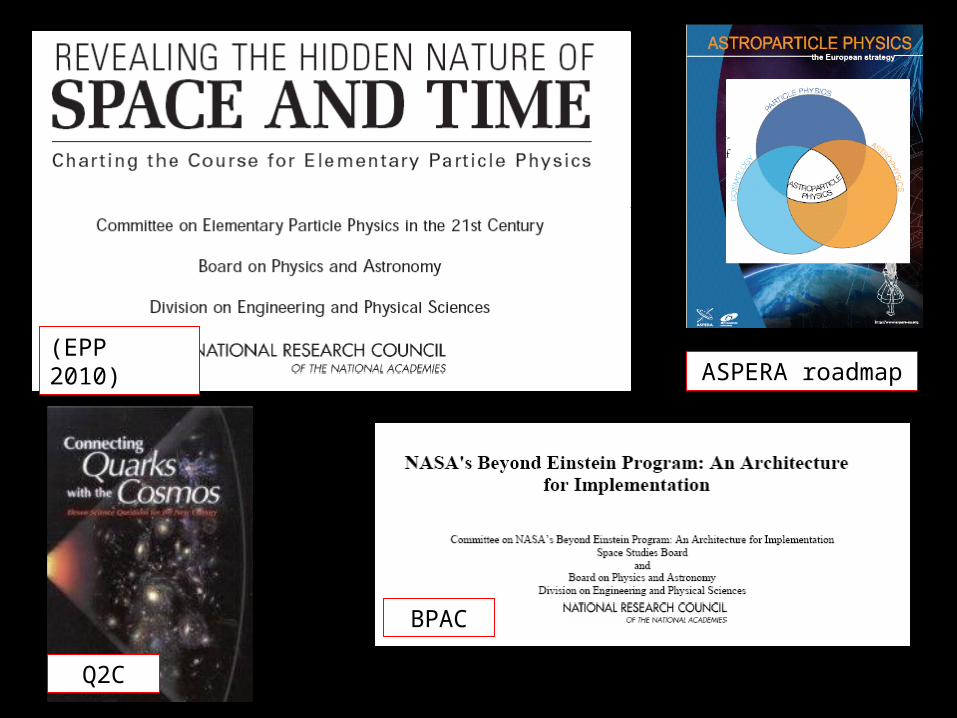
(EPP 2010)
BPAC
Q2C
ASPERA roadmap
(EPP 2010)
BPAC
Q2C
ASPERA roadmap

?
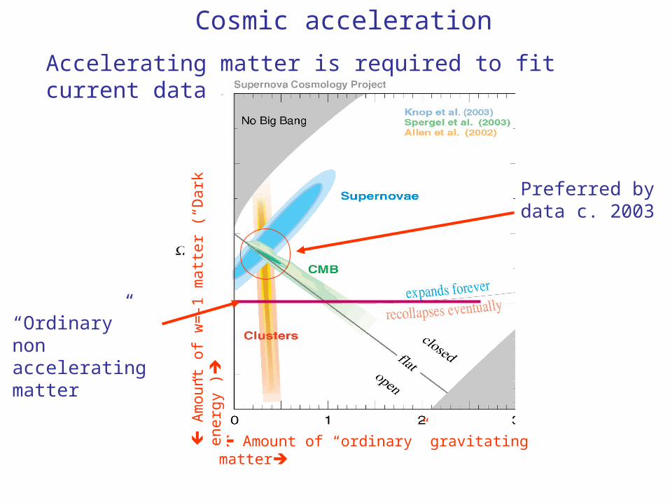
Supernova
Preferred by data c. 2003
Amount of “ordinary” gravitating matter A
mount
of
w=
-1 m
att
er
(“D
ark
energ
y”)
“Ordinary” non accelerating matter
Cosmic acceleration
Accelerating matter is required to fit current data

Cosmic acceleration
Accelerating matter is required to fit current data
Supernova Amount of “ordinary” gravitating matter A
mount
of
w=
-1 m
att
er
(“D
ark
energ
y”)
“Ordinary” non accelerating matter
Preferred by data c. 2008
BAO
Kowalski, et al., Ap.J.. (2008)
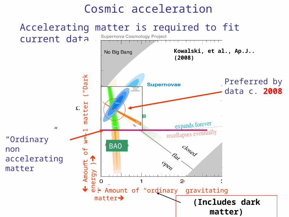
Cosmic acceleration
Accelerating matter is required to fit current data
Supernova Amount of “ordinary” gravitating matter A
mount
of
w=
-1 m
att
er
(“D
ark
energ
y”)
“Ordinary” non accelerating matter
Preferred by data c. 2008
BAO
Kowalski, et al., Ap.J.. (2008)
(Includes dark matter)
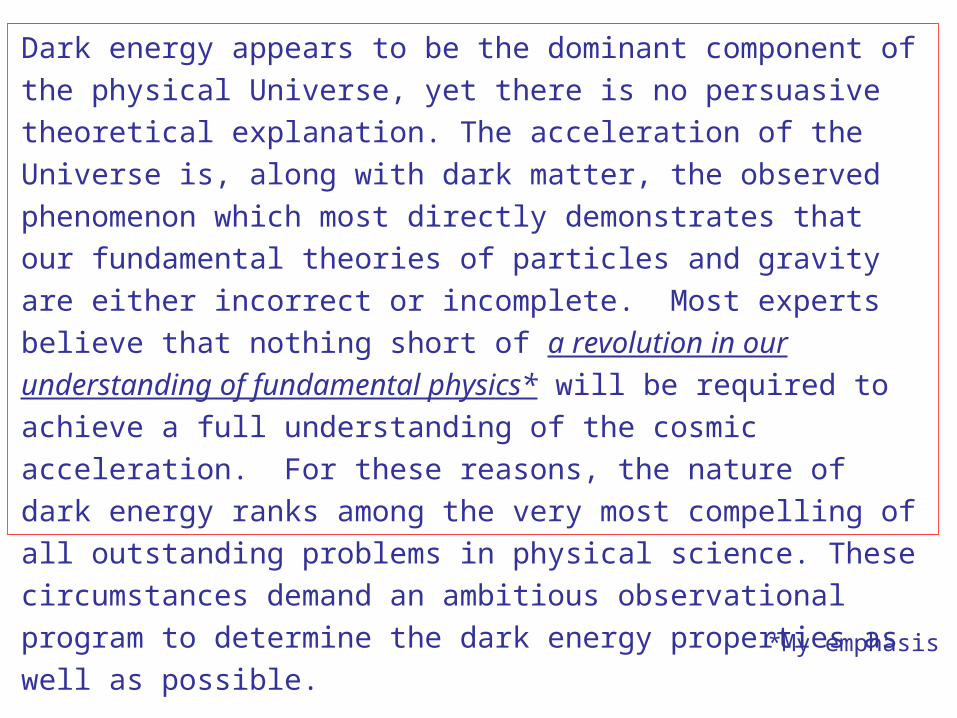
Dark energy appears to be the dominant component of the physical
Universe, yet there is no persuasive theoretical explanation. The
acceleration of the Universe is, along with dark matter, the observed
phenomenon which most directly demonstrates that our fundamental
theories of particles and gravity are either incorrect or incomplete.
Most experts believe that nothing short of a revolution in our
understanding of fundamental physics* will be required to achieve a
full understanding of the cosmic acceleration. For these reasons, the
nature of dark energy ranks among the very most compelling of all
outstanding problems in physical science. These circumstances
demand an ambitious observational program to determine the dark
energy properties as well as possible.
From the Dark Energy Task Force report (2006)www.nsf.gov/mps/ast/detf.jsp,
astro-ph/0690591*My emphasis
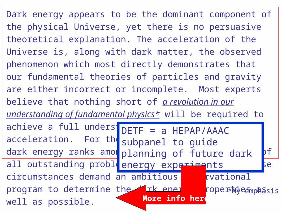
DETF = a HEPAP/AAAC subpanel to guide planning of future dark energy experiments
More info here
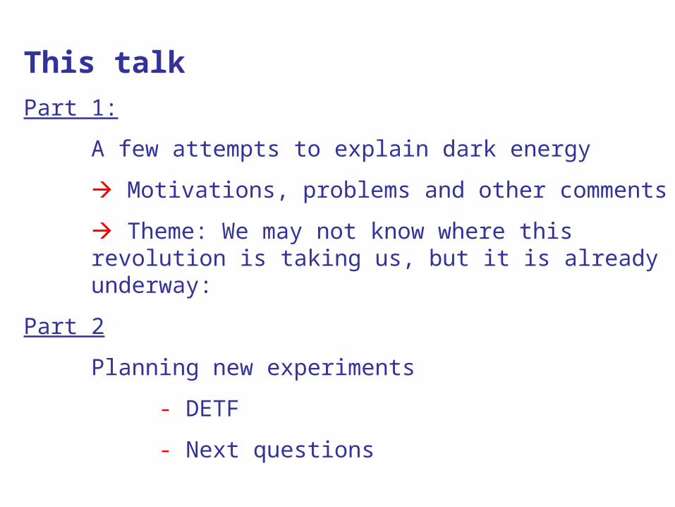
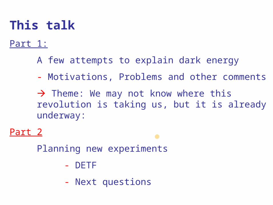
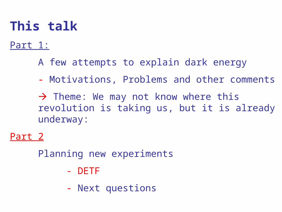
This talk
Part 1:
A few attempts to explain dark energy
Motivations, problems and other comments
Theme: We may not know where this revolution is taking us, but it is already underway:
Part 2
Planning new experiments
- DETF
- Next questions

Some general issues:
Properties:
Solve GR for the scale factor a of the Universe (a=1 today):
Positive acceleration clearly requires
• (unlike any known constituent of the Universe) or
• a non-zero cosmological constant or
• an alteration to General Relativity.
/ 1/ 3w p
43
3 3
a Gp
a

• Today,
• Many field models require a particle mass of
Some general issues:
Numbers:
4120 4 310 10DE PM eV
31010Qm eV H 2 2
Q P DEm M from

• Today,
• Many field models require a particle mass of
Some general issues:
Numbers:
4120 4 310 10DE PM eV
31010Qm eV H 2 2
Q P DEm M from
Where do these come from and how are they protected from quantum corrections?

Some general issues:
Properties:
Solve GR for the scale factor a of the Universe (a=1 today):
Positive acceleration clearly requires
• (unlike any known constituent of the Universe) or
• a non-zero cosmological constant or
• an alteration to General Relativity.
/ 1/ 3w p
43
3 3
a Gp
a
/ 1/ 3w p
Two “familiar” ways to achieve acceleration:
1) Einstein’s cosmological constant and relatives
2) Whatever drove inflation: Dynamical, Scalar field?
1w
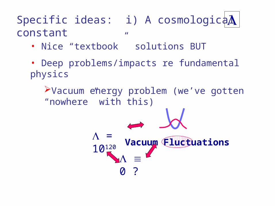
Specific ideas: i) A cosmological constant
• Nice “textbook” solutions BUT
• Deep problems/impacts re fundamental physics
Vacuum energy problem (we’ve gotten “nowhere” with this)
= 10120
0 ?
Vacuum Fluctuations
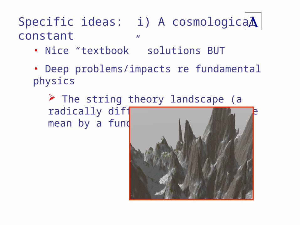
Specific ideas: i) A cosmological constant
• Nice “textbook” solutions BUT
• Deep problems/impacts re fundamental physics
The string theory landscape (a radically different idea of what we mean by a fundamental theory)

Specific ideas: i) A cosmological constant
• Nice “textbook” solutions BUT
• Deep problems/impacts re fundamental physics
The string theory landscape (a radically different idea of what we mean by a fundamental theory)
“Theory of Everything”
“Theory of Anything”
?

Specific ideas: i) A cosmological constant
• Nice “textbook” solutions BUT
• Deep problems/impacts re fundamental physics
The string theory landscape (a radically different idea of what we mean by a fundamental theory)
Not exactly a cosmological
constant
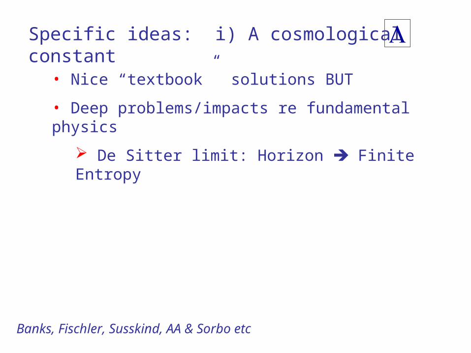
Specific ideas: i) A cosmological constant
• Nice “textbook” solutions BUT
• Deep problems/impacts re fundamental physics
De Sitter limit: Horizon Finite Entropy
Banks, Fischler, Susskind, AA & Sorbo etc

2 1S A H
“De Sitter Space: The ultimate equilibrium for the universe?
Horizon
Quantum effects: Hawking Temperature
8
3 DE
GT H
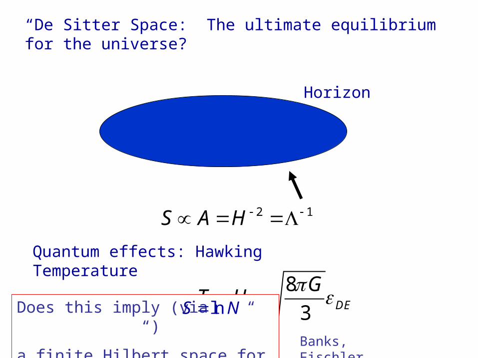
2 1S A H
“De Sitter Space: The ultimate equilibrium for the universe?
Horizon
Quantum effects: Hawking Temperature
8
3 DE
GT H
Does this imply (via “ “)
a finite Hilbert space for physics?
lnS N
Banks, Fischler
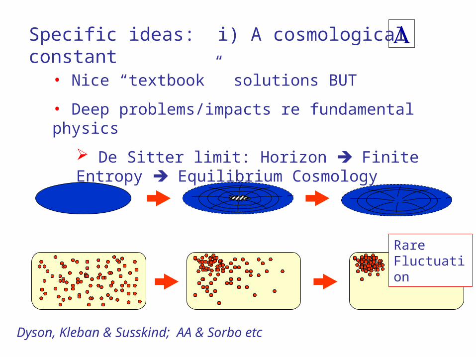
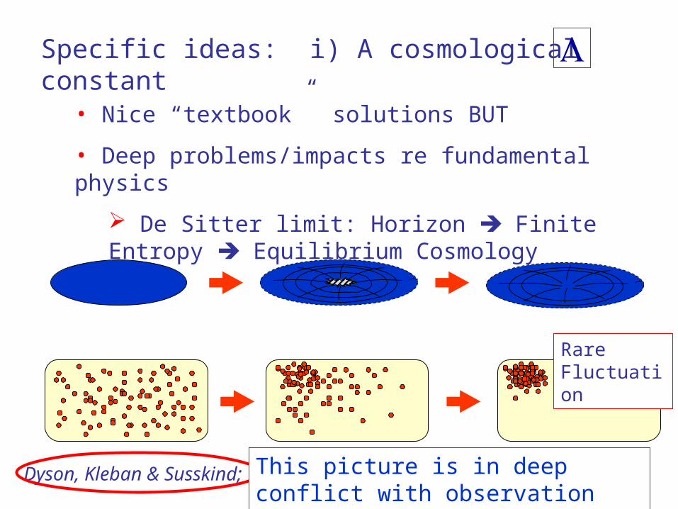
Specific ideas: i) A cosmological constant
• Nice “textbook” solutions BUT
• Deep problems/impacts re fundamental physics
De Sitter limit: Horizon Finite Entropy Equilibrium Cosmology
Rare Fluctuation
Dyson, Kleban & Susskind; AA & Sorbo etc

Specific ideas: i) A cosmological constant
• Nice “textbook” solutions BUT
• Deep problems/impacts re fundamental physics
De Sitter limit: Horizon Finite Entropy Equilibrium Cosmology
Rare Fluctuation
“Boltzmann’s Brain” ?
Dyson, Kleban & Susskind; AA & Sorbo etc
Specific ideas: i) A cosmological constant
• Nice “textbook” solutions BUT
• Deep problems/impacts re fundamental physics
De Sitter limit: Horizon Finite Entropy Equilibrium Cosmology
Rare Fluctuation
Dyson, Kleban & Susskind; AA & Sorbo etcThis picture is in deep conflict with observation

Specific ideas: i) A cosmological constant
• Nice “textbook” solutions BUT
• Deep problems/impacts re fundamental physics
De Sitter limit: Horizon Finite Entropy Equilibrium Cosmology
Rare Fluctuation
Dyson, Kleban & Susskind; AA & Sorbo etcThis picture is in deep conflict with observation (resolved by landscape?)

Specific ideas: i) A cosmological constant
• Nice “textbook” solutions BUT
• Deep problems/impacts re fundamental physics
De Sitter limit: Horizon Finite Entropy Equilibrium Cosmology
Rare Fluctuation
Dyson, Kleban & Susskind; AA & Sorbo etc
This picture forms a nice foundation for inflationary cosmology
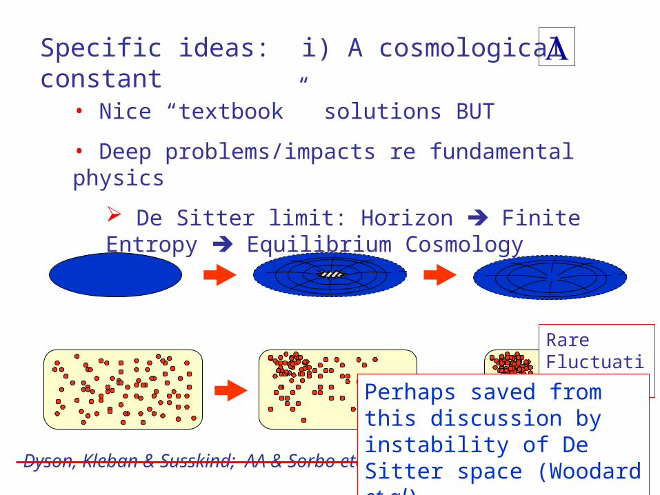
Specific ideas: i) A cosmological constant
• Nice “textbook” solutions BUT
• Deep problems/impacts re fundamental physics
De Sitter limit: Horizon Finite Entropy Equilibrium Cosmology
Rare Fluctuation
Dyson, Kleban & Susskind; AA & Sorbo etc
Perhaps saved from this discussion by instability of De Sitter space (Woodard et al)

Specific ideas: i) A cosmological constant
• Nice “textbook” solutions BUT
• Deep problems/impacts re fundamental physics
is not the “simple option”

Some general issues:
Alternative Explanations?:
Is there a less dramatic explanation of the data?

Some general issues:
Alternative Explanations?:
Is there a less dramatic explanation of the data?
For example is supernova dimming due to
• dust? (Aguirre)
• γ-axion interactions? (Csaki et al)
• Evolution of SN properties? (Drell et al)
Many of these are under increasing pressure from data, but such skepticism is critically important.
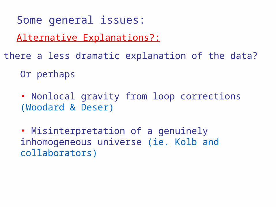
Some general issues:
Alternative Explanations?:
Is there a less dramatic explanation of the data?
Or perhaps
• Nonlocal gravity from loop corrections (Woodard & Deser)
• Misinterpretation of a genuinely inhomogeneous universe (ie. Kolb and collaborators)

• Recycle inflation ideas (resurrect dream?)
• Serious unresolved problems
Explaining/ protecting
5th force problem
Vacuum energy problem
What is the Q field? (inherited from inflation)
Why now? (Often not a separate problem)
Specific ideas: ii) A scalar field (“Quintessence”)
31010Qm eV H
0

• Recycle inflation ideas (resurrect dream?)
• Serious unresolved problems
Explaining/ protecting
5th force problem
Vacuum energy problem
What is the Q field? (inherited from inflation)
Why now? (Often not a separate problem)
Specific ideas: ii) A scalar field (“Quintessence”)
31010Qm eV H
0 Inspired by

• Recycle inflation ideas (resurrect dream?)
• Serious unresolved problems
Explaining/ protecting
5th force problem
Vacuum energy problem
What is the Q field? (inherited from inflation)
Why now? (Often not a separate problem)
Specific ideas: ii) A scalar field (“Quintessence”)
31010Qm eV H
0 Result?

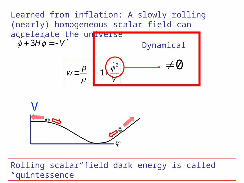
V
Learned from inflation: A slowly rolling (nearly) homogeneous scalar field can accelerate the universe
3H V
2
1p
wV

V
Learned from inflation: A slowly rolling (nearly) homogeneous scalar field can accelerate the universe
3H V
2
1p
wV
Dynamical
0
V
Learned from inflation: A slowly rolling (nearly) homogeneous scalar field can accelerate the universe
3H V
2
1p
wV
Dynamical
0
Rolling scalar field dark energy is called “quintessence”

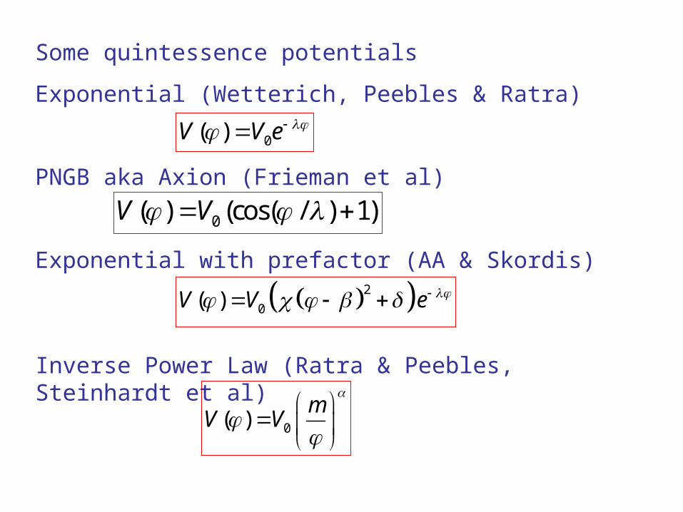
Some quintessence potentials
Exponential (Wetterich, Peebles & Ratra)
PNGB aka Axion (Frieman et al)
Exponential with prefactor (AA & Skordis)
Inverse Power Law (Ratra & Peebles, Steinhardt et al)
Some quintessence potentials
Exponential (Wetterich, Peebles & Ratra)
PNGB aka Axion (Frieman et al)
Exponential with prefactor (AA & Skordis)
0( )V V e
0( ) (cos( / ) 1)V V
2
0( )V V e
0( )m
V V
Inverse Power Law (Ratra & Peebles, Steinhardt et al)

The potentials
Exponential (Wetterich, Peebles & Ratra)
PNGB aka Axion (Frieman et al)
Exponential with prefactor (AA & Skordis)
0( )V V e
0( ) (cos( / ) 1)V V
2
0( )V V e
0( )m
V V
Inverse Power Law (Ratra & Peebles, Steinhardt et al)
Stronger than average
motivations & interest

0.2 0.4 0.6 0.8 1-1
-0.9
-0.8
-0.7
-0.6
-0.5
a
w(a
)
PNGBEXPITAS
…they cover a variety of behavior.
a = “cosmic scale factor” ≈ time

Dark energy and the ego test

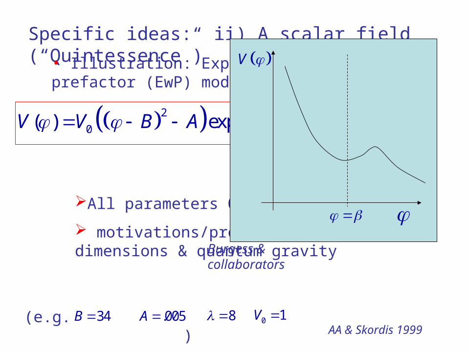
Specific ideas: ii) A scalar field (“Quintessence”)
• Illustration: Exponential with prefactor (EwP) models:
All parameters O(1) in Planck units,
motivations/protections from extra dimensions & quantum gravity
2
0( ) exp /V V B A
AA & Skordis 1999
Burgess & collaborators
(e.g. ) 34B .005A 8 0 1V
Specific ideas: ii) A scalar field (“Quintessence”)
• Illustration: Exponential with prefactor (EwP) models:
All parameters O(1) in Planck units,
motivations/protections from extra dimensions & quantum gravity
2
0( ) exp /V V B A
AA & Skordis 1999
Burgess & collaborators
(e.g. ) 34B .005A 8 0 1V
V
AA & Skordis 1999

Specific ideas: ii) A scalar field (“Quintessence”)
• Illustration: Exponential with prefactor (EwP) models:
AA & Skordis 199910
-2010
0-1.5
-1
-0.5
0
0.5
1
a
,
w
r
m
D
w

Specific ideas: iii) A mass varying neutrinos (“MaVaNs”)
• Exploit
• Issues Origin of “acceleron” (varies neutrino mass, accelerates the universe)
gravitational collapse
1/ 4 310DEm eV
Faradon, Nelson & Weiner
Afshordi et al 2005
Spitzer 2006

Specific ideas: iii) A mass varying neutrinos (“MaVaNs”)
• Exploit
• Issues Origin of “acceleron” (varies neutrino mass, accelerates the universe)
gravitational collapse
1/ 4 310DEm eV
Faradon, Nelson & Weiner
Afshordi et al 2005
Spitzer 2006
“ ”

Specific ideas: iii) A mass varying neutrinos (“MaVaNs”)
• Exploit
• Issues Origin of “acceleron” (varies neutrino mass, accelerates the universe)
gravitational collapse
1/ 4 310DEm eV
Faradon, Nelson & Weiner
Afshordi et al 2005
Spitzer 2006
“ ”

Specific ideas: iv) Modify Gravity
• Not something to be done lightly, but given our confusion about cosmic acceleration, well worth considering.
• Many deep technical issues
e.g. DGP (Dvali, Gabadadze and Porrati)
Charmousis et alGhosts

Specific ideas: iv) Modify Gravity
• Not something to be done lightly, but given our confusion about cosmic acceleration, well worth considering.
• Many deep technical issues
e.g. DGP (Dvali, Gabadadze and Porrati)
Charmousis et alGhosts
See “Origins of Dark Energy” meeting May 07 for numerous talks

This talk
Part 1:
A few attempts to explain dark energy
- Motivations, Problems and other comments
Theme: We may not know where this revolution is taking us, but it is already underway:
Part 2
Planning new experiments
- DETF
- Next questions

This talk
Part 1:
A few attempts to explain dark energy
- Motivations, Problems and other comments
Theme: We may not know where this revolution is taking us, but it is already underway:
Part 2
Planning new experiments
- DETF
- Next questions
This talk
Part 1:
A few attempts to explain dark energy
- Motivations, Problems and other comments
Theme: We may not know where this revolution is taking us, but it is already underway:
Part 2
Planning new experiments
- DETF
- Next questions
This talk
Part 1:
A few attempts to explain dark energy
- Motivations, Problems and other comments
Theme: We may not know where this revolution is taking us, but it is already underway:
Part 2
Planning new experiments
- DETF
- Next questions
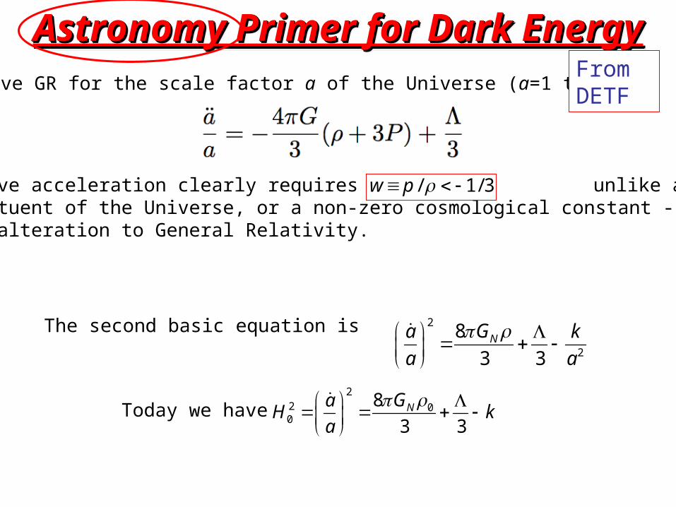
Astronomy Primer for Dark EnergyAstronomy Primer for Dark EnergyAstronomy Primer for Dark EnergyAstronomy Primer for Dark EnergySolve GR for the scale factor a of the Universe (a=1 today):
Positive acceleration clearly requires unlike any knownconstituent of the Universe, or a non-zero cosmological constant - or an alteration to General Relativity.
2
2
8
3 3NGa k
a a
The second basic equation is
Today we have2
2 00
8
3 3NGa
H ka
/ 1/ 3w p
From DETF

Hubble ParameterHubble Parameter
18GN03H0
2 3H0
2 k
H02 k
We can rewrite this as
To get the generalization that applies not just now (a=1), we needto distinguish between non-relativistic matter and relativistic matter.We also generalize to dark energy with a constant w, not necessarily equal to -1:
Dark Energy
curvature
rel. matter
non-rel. matter
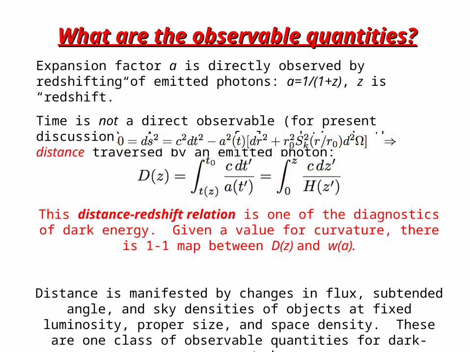
What are the observable quantities?What are the observable quantities?Expansion factor a is directly observed by redshifting of emitted photons: a=1/(1+z), z is “redshift.”
Time is not a direct observable (for present discussion). A measure of elapsed time is the distance traversed by an emitted photon:
This distance-redshift relation is one of the diagnostics of dark energy. Given a value for curvature, there is 1-1 map between D(z) and w(a).
Distance is manifested by changes in flux, subtended angle, and sky densities of objects at fixed luminosity, proper size, and space density.
These are one class of observable quantities for dark-energy study.

Another observable quantity:Another observable quantity:The progress of gravitational collapse is damped by expansion of the Universe. Density fluctuations arising from inflation-era quantum fluctuations increase their amplitude with time. Quantify this by the growth factor g of density fluctuations in linear perturbation theory. GR gives:
This growth-redshift relation is the second diagnostic of dark energy. If GR is correct, there is 1-1 map between D(z) and g(z).
If GR is incorrect, observed quantities may fail to obey this relation.
Growth factor is determined by measuring the density fluctuations in nearby dark matter (!), comparing to those seen at z=1088 by WMAP.

What are the observable quantities?What are the observable quantities?
Future dark-energy experiments will require percent-level precision onthe primary observables D(z) and g(z).
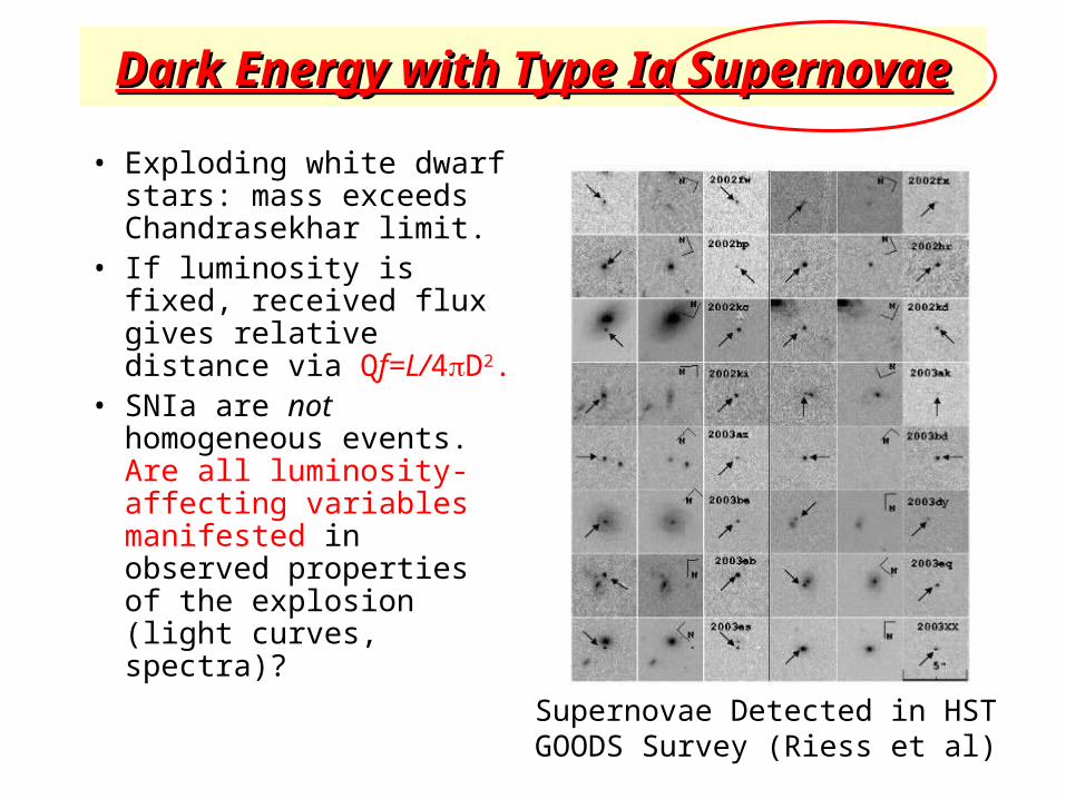
Dark Energy with Type Ia SupernovaeDark Energy with Type Ia Supernovae
• Exploding white dwarf stars: mass exceeds Chandrasekhar limit.
• If luminosity is fixed, received flux gives relative distance via Qf=L/4D2.
• SNIa are not homogeneous events. Are all luminosity-affecting variables manifested in observed properties of the explosion (light curves, spectra)? Supernovae Detected in HST
GOODS Survey (Riess et al)
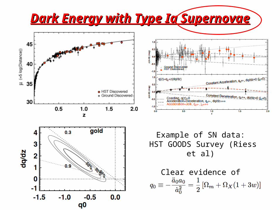
Dark Energy with Type Ia SupernovaeDark Energy with Type Ia Supernovae
Example of SN data: HST GOODS Survey (Riess et
al)
Clear evidence of acceleration!
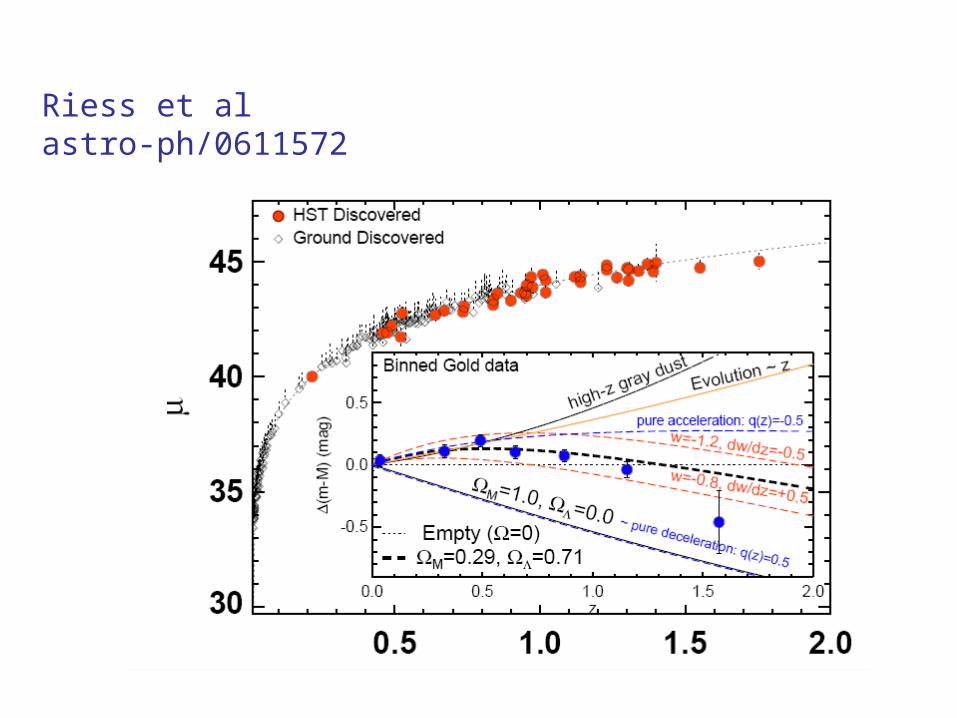
Riess et al astro-ph/0611572

Dark Energy with Baryon Acoustic OscillationsDark Energy with Baryon Acoustic Oscillations
•Acoustic waves propagate in the baryon-photon plasma starting at end of inflation.
•When plasma combines to neutral hydrogen, sound propagation ends.
•Cosmic expansion sets up a predictable standing wave pattern on scales of the Hubble length. The Hubble length (~sound horizon rs) ~140 Mpc is imprinted on the matter density pattern.
•Identify the angular scale subtending rs then use s=rs/D(z)
•WMAP/Planck determine rs and the distance to z=1088.
•Survey of galaxies (as signposts for dark matter) recover D(z), H(z) at 0<z<5.
•Galaxy survey can be visible/NIR or 21-cm emission
BAO seen in CMB(WMAP)
BAO seen in SDSSGalaxy correlations
(Eisenstein et al)

Dark Energy with Galaxy ClustersDark Energy with Galaxy Clusters•Galaxy clusters are the largest structures in Universe to undergo gravitational collapse.
•Markers for locations with density contrast above a critical value.
•Theory predicts the mass function dN/dMdV. We observe dN/dzd.
•Dark energy sensitivity:
•Mass function is very sensitive to M; very sensitive to g(z).
•Also very sensitive to mis-estimation of mass, which is not directly observed.
Optical View(Lupton/SDSS)
Cluster method probes both D(z) and g(z)

Dark Energy with Galaxy ClustersDark Energy with Galaxy Clusters
30 GHz View(Carlstrom et al)
Sunyaev-Zeldovich effect
X-ray View(Chandra)
Optical View(Lupton/SDSS)
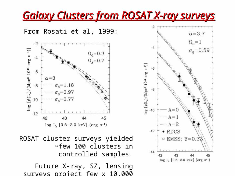
Galaxy Clusters from ROSAT X-ray surveysGalaxy Clusters from ROSAT X-ray surveys
ROSAT cluster surveys yielded ~few 100 clusters in controlled samples.
Future X-ray, SZ, lensing surveys project few x 10,000 detections.
From Rosati et al, 1999:
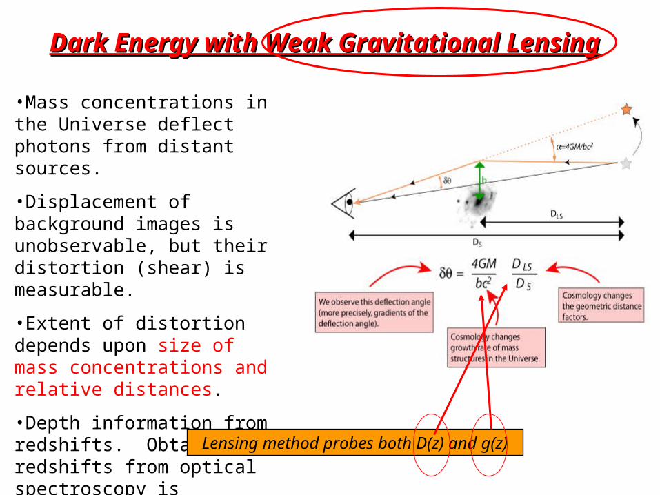
Dark Energy with Weak Gravitational LensingDark Energy with Weak Gravitational Lensing
•Mass concentrations in the Universe deflect photons from distant sources.
•Displacement of background images is unobservable, but their distortion (shear) is measurable.
•Extent of distortion depends upon size of mass concentrations and relative distances.
•Depth information from redshifts. Obtaining 108 redshifts from optical spectroscopy is infeasible. “photometric” redshifts instead.
Lensing method probes both D(z) and g(z)

Dark Energy with Weak Gravitational LensingDark Energy with Weak Gravitational Lensing
In weak lensing, shapes of galaxies are measured. Dominant noise source is the (random) intrinsic shape of galaxies. Large-N statistics extract lensing influence from intrinsic noise.


Choose your background photon source:Choose your background photon source:
QuickTime™ and aTIFF (Uncompressed) decompressor
are needed to see this picture.
Faint background galaxies:
Use visible/NIR imaging to determine shapes.
Photometric redshifts.
Photons from the CMB:
Use mm-wave high-resolution imaging of CMB.
All sources at z=1088.
21-cm photons:
Use the proposed Square Kilometer Array (SKA).
Sources are neutral H in regular galaxies at z<2, or the neutral Universe at z>6.
(lensing not yet detected)
(lensing not yet detected)
Hoekstra et al 2006:
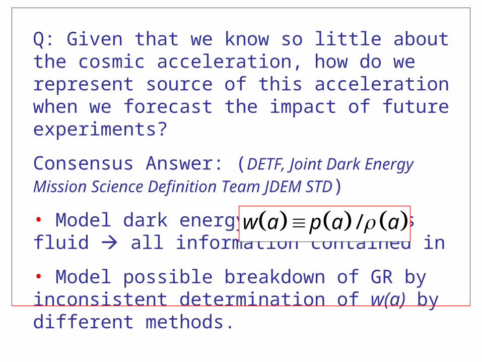
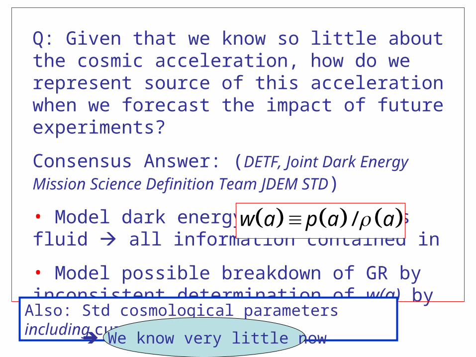
Q: Given that we know so little about the cosmic acceleration, how do we represent source of this acceleration when we forecast the impact of future experiments?
Consensus Answer: (DETF, Joint Dark Energy Mission
Science Definition Team JDEM STD)
• Model dark energy as homogeneous fluid all information contained in
• Model possible breakdown of GR by inconsistent determination of w(a) by different methods.
/w a p a a
Also: Std cosmological parameters including curvature
Q: Given that we know so little about the cosmic acceleration, how do we represent source of this acceleration when we forecast the impact of future experiments?
Consensus Answer: (DETF, Joint Dark Energy Mission
Science Definition Team JDEM STD)
• Model dark energy as homogeneous fluid all information contained in
• Model possible breakdown of GR by inconsistent determination of w(a) by different methods.
/w a p a a
Also: Std cosmological parameters including curvature We know very little now

Some general issues:
Properties:
Solve GR for the scale factor a of the Universe (a=1 today):
Positive acceleration clearly requires
• (unlike any known constituent of the Universe) or
• a non-zero cosmological constant or
• an alteration to General Relativity.
/ 1/ 3w p
43
3 3
a Gp
a
Two “familiar” ways to achieve acceleration:
1) Einstein’s cosmological constant and relatives
2) Whatever drove inflation: Dynamical, Scalar field?
/ 1/ 3w p
1w
Recall:
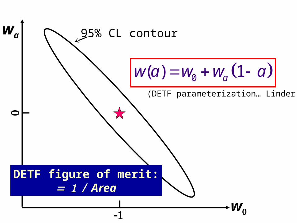
w
wa
DETF figure of merit:Area
95% CL contour
(DETF parameterization… Linder)
0( ) 1aw a w w a

The DETF stages (data models constructed for each one)
Stage 2: Underway
Stage 3: Medium size/term projects
Stage 4: Large longer term projects (ie JDEM, LST)
DETF modeled
• SN
•Weak Lensing
•Baryon Oscillation
•Cluster data
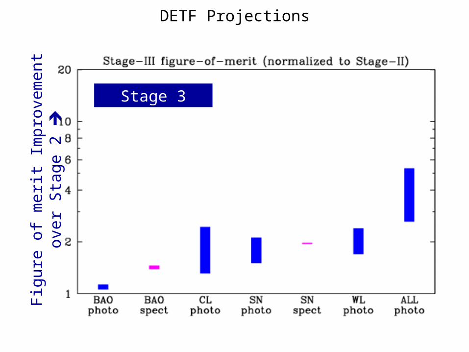
DETF Projections
Stage 3
Fig
ure
of m
erit
Impr
ovem
ent
over
S
tage
2
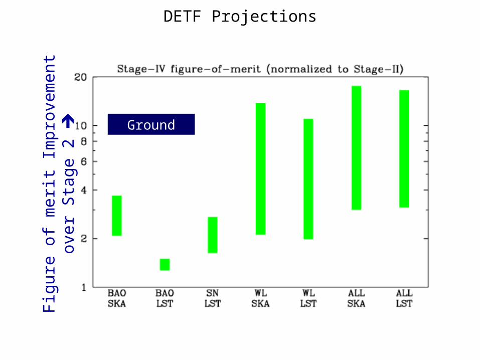
DETF Projections
Ground
Fig
ure
of m
erit
Impr
ovem
ent
over
S
tage
2
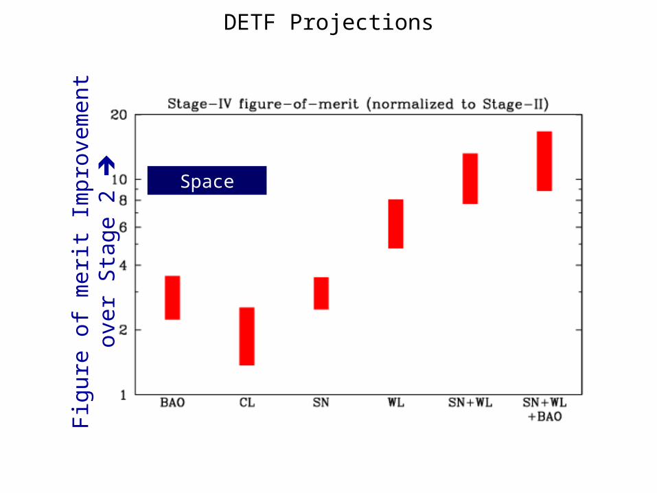
DETF Projections
Space
Fig
ure
of m
erit
Impr
ovem
ent
over
S
tage
2
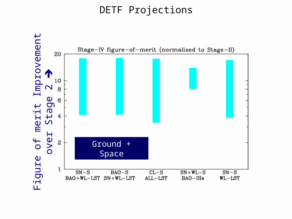
DETF Projections
Ground + Space
Fig
ure
of m
erit
Impr
ovem
ent
over
S
tage
2
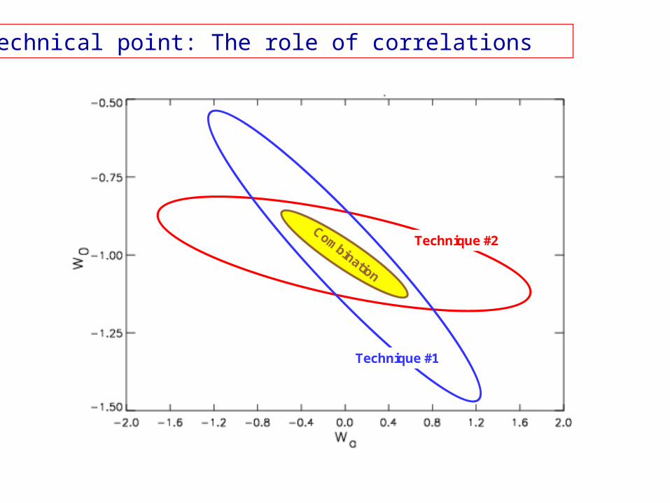
Combination
Technique #2
Technique #1
A technical point: The role of correlations

From the DETF Executive Summary
One of our main findings is that no single technique can answer the outstanding questions about dark energy: combinations of at least two of these techniques must be used to fully realize the promise of future observations.
Already there are proposals for major, long-term (Stage IV) projects incorporating these techniques that have the promise of increasing our figure of merit by a factor of ten beyond the level it will reach with the conclusion of current experiments. What is urgently needed is a commitment to fund a program comprised of a selection of these projects. The selection should be made on the basis of critical evaluations of their costs, benefits, and risks.

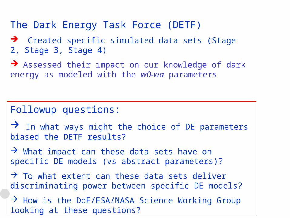
The Dark Energy Task Force (DETF)
Created specific simulated data sets (Stage 2, Stage 3, Stage 4)
Assessed their impact on our knowledge of dark energy as modeled with the w0-wa parameters
0 1aw a w w a

Followup questions:
In what ways might the choice of DE parameters biased the DETF results?
What impact can these data sets have on specific DE models (vs abstract parameters)?
To what extent can these data sets deliver discriminating power between specific DE models?
How is the DoE/ESA/NASA Science Working Group looking at these questions?
The Dark Energy Task Force (DETF)
Created specific simulated data sets (Stage 2, Stage 3, Stage 4)
Assessed their impact on our knowledge of dark energy as modeled with the w0-wa parameters

The Dark Energy Task Force (DETF)
Created specific simulated data sets (Stage 2, Stage 3, Stage 4)
Assessed their impact on our knowledge of dark energy as modeled with the w0-wa parameters
Followup questions:
In what ways might the choice of DE parameters biased the DETF results?
What impact can these data sets have on specific DE models (vs abstract parameters)?
To what extent can these data sets deliver discriminating power between specific DE models?
How is the DoE/ESA/NASA Science Working Group looking at these questions?
NB: To make concretecomparisons this work ignores
various possible improvements to the DETF data models.
(see for example J Newman, H Zhan et al
& Schneider et al)ALSO
Ground/Space synergies
DETF
The Dark Energy Task Force (DETF)
Created specific simulated data sets (Stage 2, Stage 3, Stage 4)
Assessed their impact on our knowledge of dark energy as modeled with the w0-wa parameters
Followup questions:
In what ways might the choice of DE parameters biased the DETF results?
What impact can these data sets have on specific DE models (vs abstract parameters)?
To what extent can these data sets deliver discriminating power between specific DE models?
How is the DoE/ESA/NASA Science Working Group looking at these questions?

A:
• DETF Stage 3: Poor
• DETF Stage 4: Marginal… Excellent within reach (AA)
In what ways might the choice of DE parameters have skewed the DETF results?
A: Only by an overall (possibly important) rescaling
What impact can these data sets have on specific DE models (vs abstract parameters)?
A: Very similar to DETF results in w0-wa space
Summary
To what extent can these data sets deliver discriminating power between specific DE models?

0 2 4 6 8 10 12 14 16 180
1
2
Stage 4 Space WL Opt; lin-a NGrid
= 16, zmax
= 4, Tag = 054301
i
0.2 0.3 0.4 0.5 0.6 0.7 0.8 0.9 1-1
0
1
f's
a
0.2 0.3 0.4 0.5 0.6 0.7 0.8 0.9 1-1
0
1
f's
a
0.2 0.3 0.4 0.5 0.6 0.7 0.8 0.9 1-1
0
1
f's
a
1
2
3
4
5
6
7
8
9
i
Prin
cipl
e A
xes
if i
a
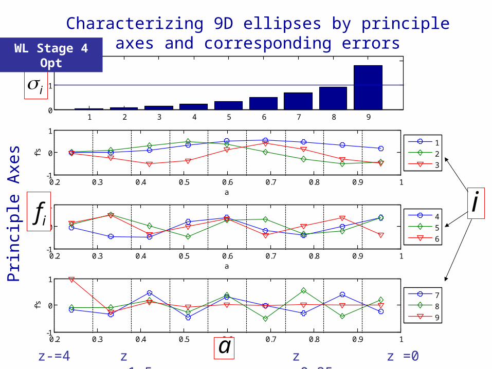
Characterizing 9D ellipses by principle axes and corresponding errorsWL Stage 4 Opt
“Convergence”z-=4 z =1.5 z =0.25 z =0

BAOp BAOs SNp SNs WLp ALLp1
10
100
1e3
1e4
Stage 3
Bska Blst Slst Wska Wlst Aska Alst1
10
100
1e3
1e4
Stage 4 Ground
BAO SN WL S+W S+W+B1
10
100
1e3
1e4
Stage 4 Space
Grid Linear in a zmax = 4 scale: 0
1
10
100
1e3
1e4
Stage 4 Ground+Space
[SSBlstW lst] [BSSlstW lst] Alllst [SSWSBIIIs] SsW lst
DETF(-CL)
9D (-CL)
DETF/9DF

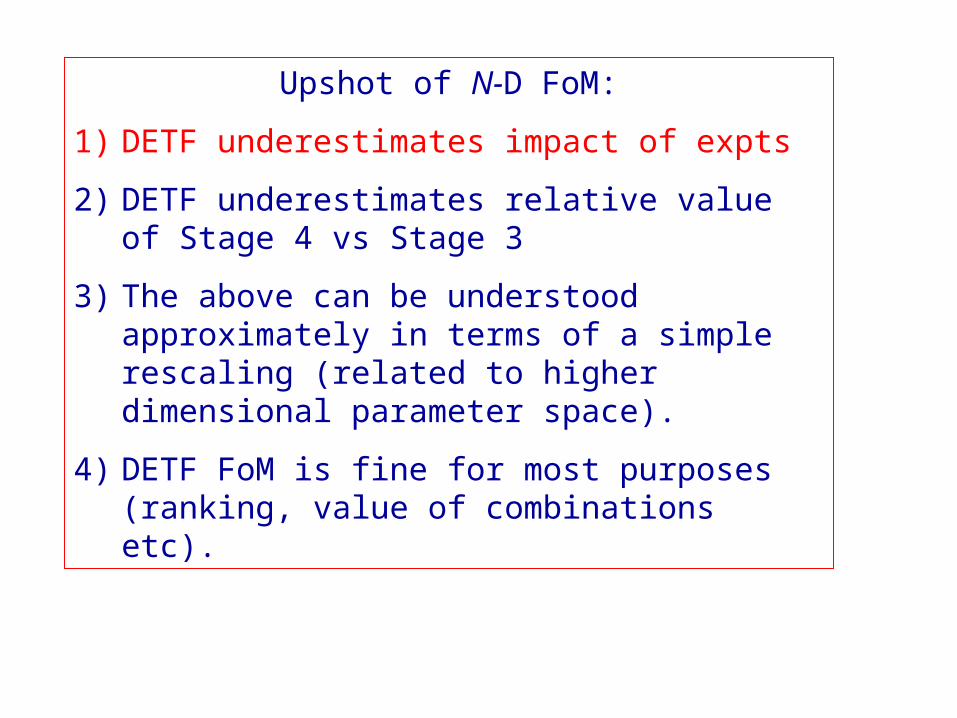
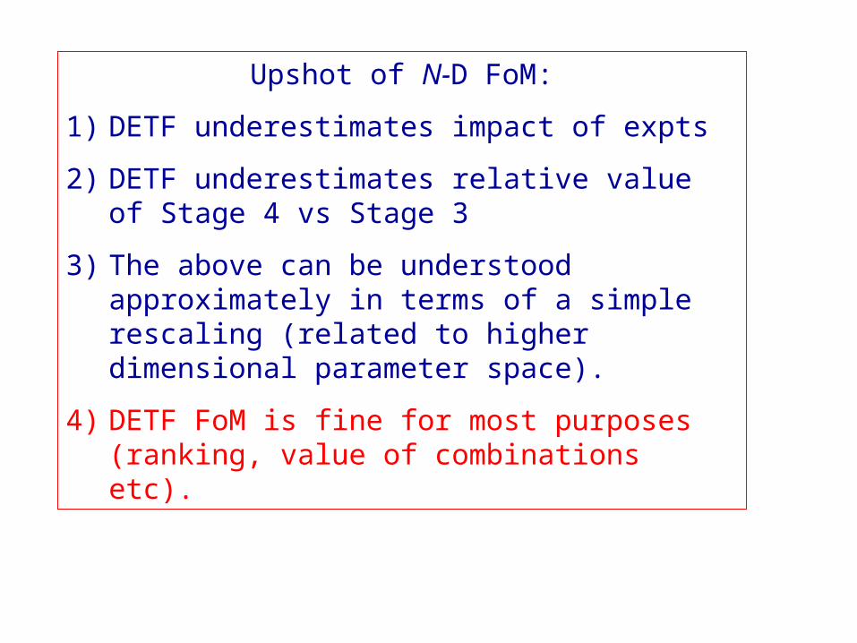
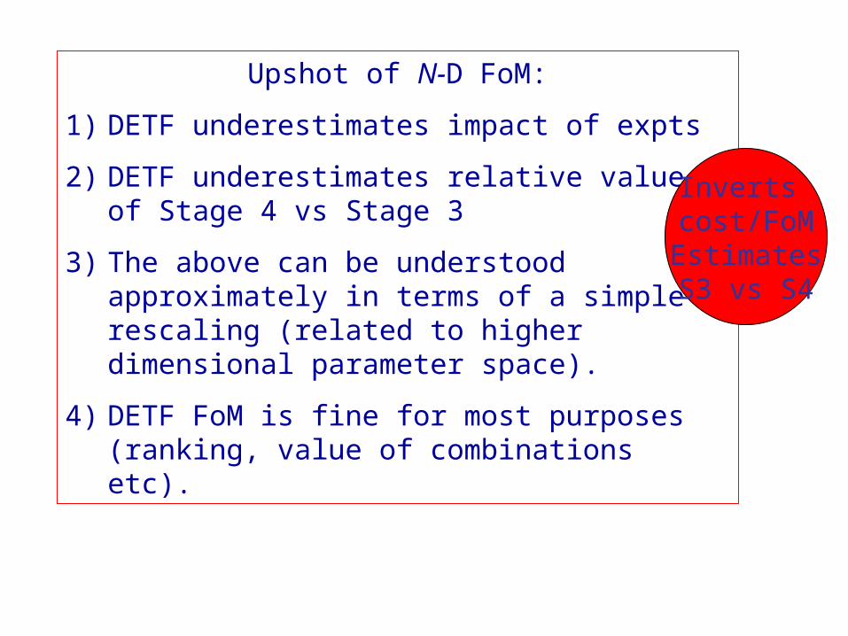
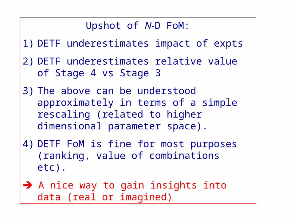
Upshot of N-D FoM:
1) DETF underestimates impact of expts
2) DETF underestimates relative value of Stage 4 vs Stage 3
3) The above can be understood approximately in terms of a simple rescaling (related to higher dimensional parameter space).
4) DETF FoM is fine for most purposes (ranking, value of combinations etc).
Inverts cost/FoMEstimatesS3 vs S4
A:
• DETF Stage 3: Poor
• DETF Stage 4: Marginal… Excellent within reach (AA)
In what ways might the choice of DE parameters have skewed the DETF results?
A: Only by an overall (possibly important) rescaling
What impact can these data sets have on specific DE models (vs abstract parameters)?
A: Very similar to DETF results in w0-wa space
Summary
To what extent can these data sets deliver discriminating power between specific DE models?

DETF stage 2
DETF stage 3
DETF stage 4
[ Abrahamse, AA, Barnard, Bozek & Yashar PRD 2008]

A:
• DETF Stage 3: Poor
• DETF Stage 4: Marginal… Excellent within reach (AA)
In what ways might the choice of DE parameters have skewed the DETF results?
A: Only by an overall (possibly important) rescaling
What impact can these data sets have on specific DE models (vs abstract parameters)?
A: Very similar to DETF results in w0-wa space
Summary
To what extent can these data sets deliver discriminating power between specific DE models?

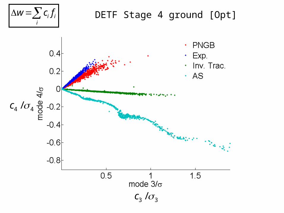
DETF Stage 4 ground [Opt]
1 1/c
2 2/c
i ii
w c f
DETF Stage 4 ground [Opt]
3 3/c
4 4/c
i ii
w c f

0.2 0.4 0.6 0.8 1-1
-0.9
-0.8
-0.7
-0.6
-0.5
a
w(a
)
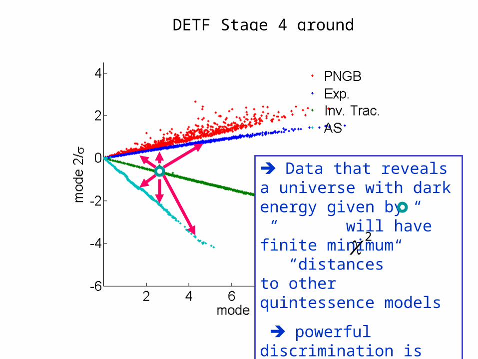
PNGBEXPITAS
The different kinds of curves correspond to different “trajectories” in mode space (similar to FT’s)

DETF Stage 4 ground
Data that reveals a universe with dark energy given by “ “ will have finite minimum “distances” to other quintessence models
powerful discrimination is possible.
2
A:
• DETF Stage 3: Poor
• DETF Stage 4: Marginal… Excellent within reach (AA)
In what ways might the choice of DE parameters have skewed the DETF results?
A: Only by an overall (possibly important) rescaling
What impact can these data sets have on specific DE models (vs abstract parameters)?
A: Very similar to DETF results in w0-wa space
Summary
To what extent can these data sets deliver discriminating power between specific DE models?
Interesting contributionto discussion of Stage 4
(if you believe scalar field modes)

How is the DoE/ESA/NASA Science Working Group looking at these questions?
i) Using w(a) eigenmodes
ii) Revealing value of higher modes
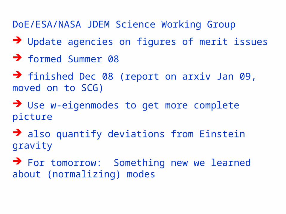
DoE/ESA/NASA JDEM Science Working Group
Update agencies on figures of merit issues
formed Summer 08
finished Dec 08 (report on arxiv Jan 09, moved on to SCG)
Use w-eigenmodes to get more complete picture
also quantify deviations from Einstein gravity
For tomorrow: Something new we learned about (normalizing) modes

How is the DoE/ESA/NASA Science Working Group looking at these questions?
i) Using w(a) eigenmodes
ii) Revealing value of higher modes

This talk
Part 1:
A few attempts to explain dark energy
- Motivations, problems and other comments
Theme: We may not know where this revolution is taking us, but it is already underway:
Part 2
Planning new experiments
- DETF
- Next questions

This talk
Part 1:
A few attempts to explain dark energy
- Motivations, problems and other comments
Theme: We may not know where this revolution is taking us, but it is already underway:
Part 2
Planning new experiments
- DETF
- Next questions
Deeply exciting physics

This talk
Part 1:
A few attempts to explain dark energy
- Motivations, problems and other comments
Theme: We may not know where this revolution is taking us, but it is already underway:
Part 2
Planning new experiments
- DETF
- Next questions
Rigorous quantitative case for “Stage 4” (i.e. LSST, JDEM, Euclid)
Advances in combining techniques
Insights into ground & space synergies
Deeply exciting physics

END

Additional Slides
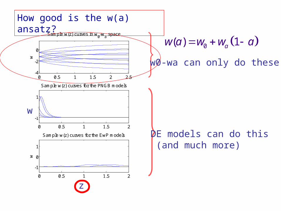
0 0.5 1 1.5 2 2.5-4
-2
0
wSample w(z) curves in w
0-w
a space
0 0.5 1 1.5 2
-1
0
1
w
Sample w(z) curves for the PNGB models
0 0.5 1 1.5 2
-1
0
1
z
w
Sample w(z) curves for the EwP models
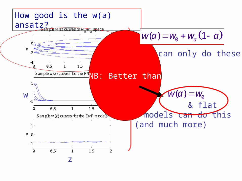
w0-wa can only do these
DE models can do this (and much more)
w
z
0( ) 1aw a w w a
How good is the w(a) ansatz?
0 0.5 1 1.5 2 2.5-4
-2
0
wSample w(z) curves in w
0-w
a space
0 0.5 1 1.5 2
-1
0
1
w
Sample w(z) curves for the PNGB models
0 0.5 1 1.5 2
-1
0
1
z
w
Sample w(z) curves for the EwP models
w0-wa can only do these
DE models can do this (and much more)
w
z
How good is the w(a) ansatz?
NB: Better than
0( ) 1aw a w w a
0( )w a w& flat

10-2
10-1
100
101
-1
0
1
z
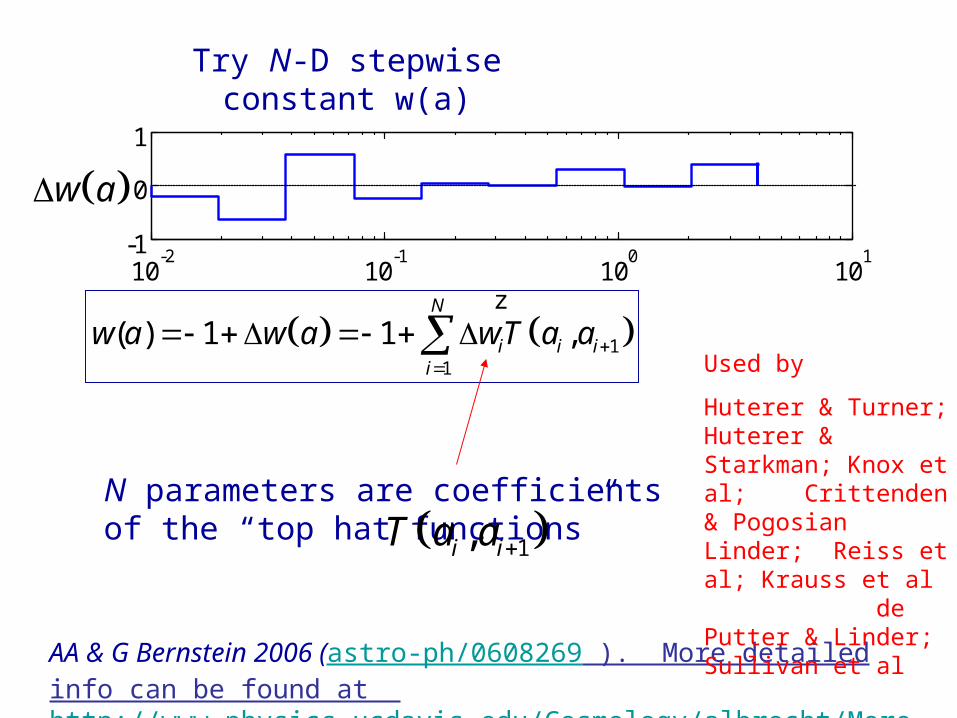
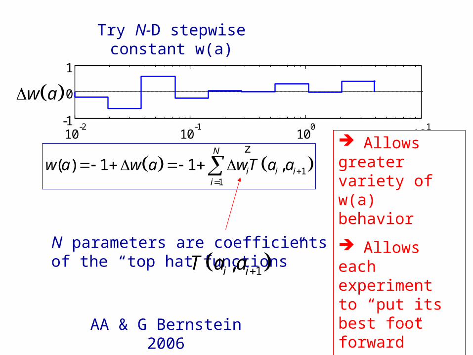
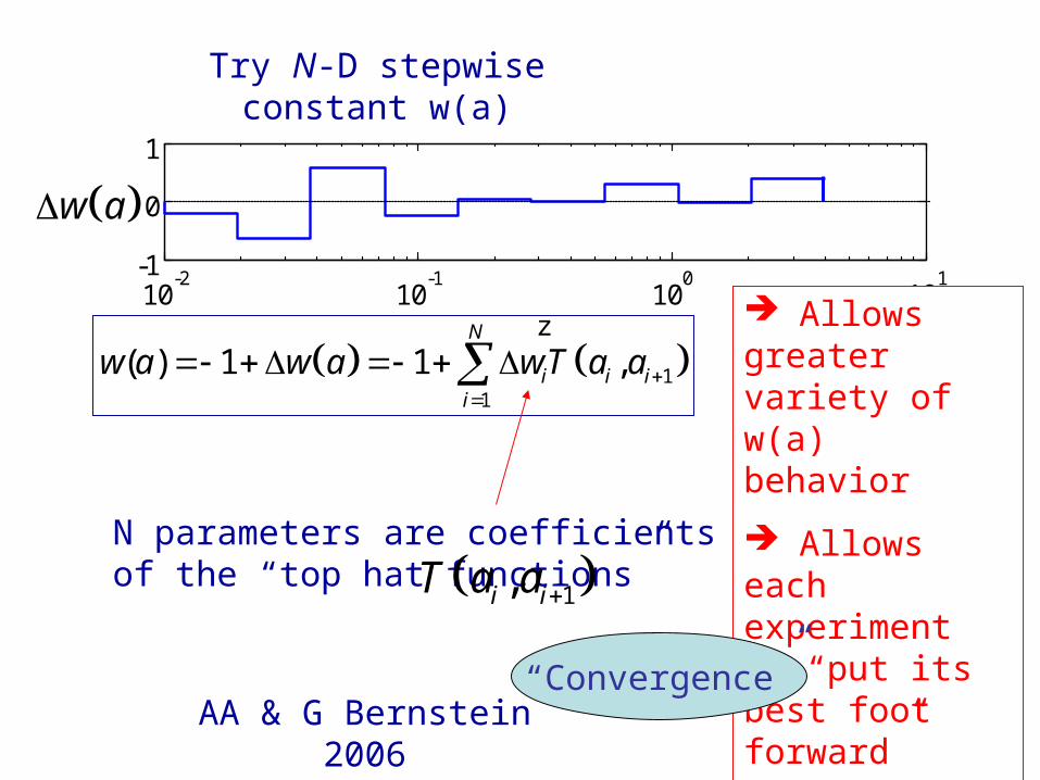
Try N-D stepwise constant w(a)
w a
AA & G Bernstein 2006 (astro-ph/0608269 ). More detailed info can be found at http://www.physics.ucdavis.edu/Cosmology/albrecht/MoreInfo0608269/
N parameters are coefficients of the “top hat functions”
11
( ) 1 1 ,N
i i ii
w a w a wT a a
1,i iT a a
10-2
10-1
100
101
-1
0
1
z
Try N-D stepwise constant w(a)
w a
AA & G Bernstein 2006 (astro-ph/0608269 ). More detailed info can be found at http://www.physics.ucdavis.edu/Cosmology/albrecht/MoreInfo0608269/
N parameters are coefficients of the “top hat functions”
11
( ) 1 1 ,N
i i ii
w a w a wT a a
1,i iT a a
Used by
Huterer & Turner; Huterer & Starkman; Knox et al; Crittenden & Pogosian Linder; Reiss et al; Krauss et al de Putter & Linder; Sullivan et al
10-2
10-1
100
101
-1
0
1
z
Try N-D stepwise constant w(a)
w a
AA & G Bernstein 2006
N parameters are coefficients of the “top hat functions”
11
( ) 1 1 ,N
i i ii
w a w a wT a a
1,i iT a a
Allows greater variety of w(a) behavior
Allows each experiment to “put its best foot forward”
Any signal rejects Λ
10-2
10-1
100
101
-1
0
1
z
Try N-D stepwise constant w(a)
w a
AA & G Bernstein 2006
N parameters are coefficients of the “top hat functions”
11
( ) 1 1 ,N
i i ii
w a w a wT a a
1,i iT a a
Allows greater variety of w(a) behavior
Allows each experiment to “put its best foot forward”
Any signal rejects Λ“Convergence”

2D illustration:
1
2
Axis 1
Axis 2
1f
2f
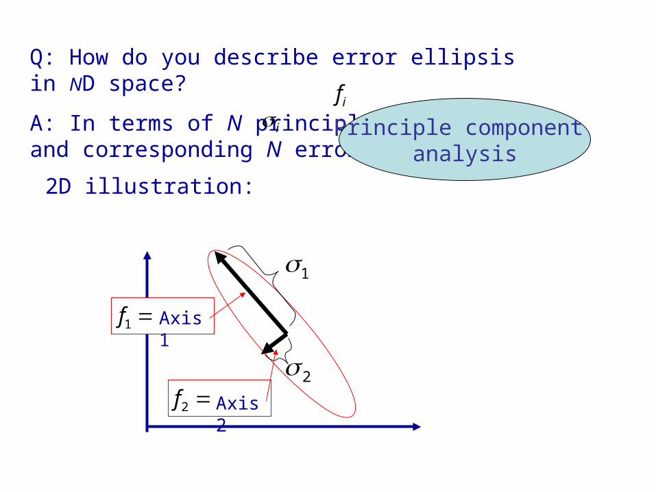
Q: How do you describe error ellipsis in ND space?
A: In terms of N principle axes and corresponding N errors :
if
i
Q: How do you describe error ellipsis in ND space?
A: In terms of N principle axes and corresponding N errors :
2D illustration:
if
i
1
2
Axis 1
Axis 2
1f
2f
Principle component analysis
2D illustration:
1
2
Axis 1
Axis 2
1f
2f
NB: in general the s form a complete basis:
i ii
w c f
if
The are independently measured qualities with errors
ic
i
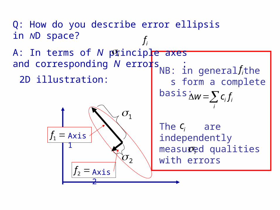
Q: How do you describe error ellipsis in ND space?
A: In terms of N principle axes and corresponding N errors :
if
i

2D illustration:
1
2
Axis 1
Axis 2
1f
2f
NB: in general the s form a complete basis:
i ii
w c f
if
The are independently measured qualities with errors
ic
i
Q: How do you describe error ellipsis in ND space?
A: In terms of N principle axes and corresponding N errors :
if
i

1 2 3 4 5 6 7 8 90
1
2
Stage 2 ; lin-a NGrid
= 9, zmax
= 4, Tag = 044301
i
0.2 0.3 0.4 0.5 0.6 0.7 0.8 0.9 1-1
0
1
f's
a
1
2
3
0.2 0.3 0.4 0.5 0.6 0.7 0.8 0.9 1-1
0
1
f's
a
4
5
6
0.2 0.3 0.4 0.5 0.6 0.7 0.8 0.9 1-1
0
1
f's
a
7
8
9
i
Prin
cipl
e A
xes
if i
a
Characterizing 9D ellipses by principle axes and corresponding errorsDETF stage 2
z-=4 z =1.5 z =0.25 z =0
1 2 3 4 5 6 7 8 90
1
2
Stage 4 Space WL Opt; lin-a NGrid
= 9, zmax
= 4, Tag = 044301
i
0.2 0.3 0.4 0.5 0.6 0.7 0.8 0.9 1-1
0
1
f's
a
0.2 0.3 0.4 0.5 0.6 0.7 0.8 0.9 1-1
0
1
f's
a
0.2 0.3 0.4 0.5 0.6 0.7 0.8 0.9 1-1
0
1
f's
a
1
2
3
4
5
6
7
8
9
i
Prin
cipl
e A
xes
if i
a
Characterizing 9D ellipses by principle axes and corresponding errorsWL Stage 4 Opt
z-=4 z =1.5 z =0.25 z =0

0 2 4 6 8 10 12 14 16 180
1
2
Stage 4 Space WL Opt; lin-a NGrid
= 16, zmax
= 4, Tag = 054301
i
0.2 0.3 0.4 0.5 0.6 0.7 0.8 0.9 1-1
0
1
f's
a
0.2 0.3 0.4 0.5 0.6 0.7 0.8 0.9 1-1
0
1
f's
a
0.2 0.3 0.4 0.5 0.6 0.7 0.8 0.9 1-1
0
1
f's
a
1
2
3
4
5
6
7
8
9
i
Prin
cipl
e A
xes
if i
a
Characterizing 9D ellipses by principle axes and corresponding errorsWL Stage 4 Opt
“Convergence”z-=4 z =1.5 z =0.25 z =0

BAOp BAOs SNp SNs WLp ALLp1
10
100
1e3
1e4
Stage 3
Bska Blst Slst Wska Wlst Aska Alst1
10
100
1e3
1e4
Stage 4 Ground
BAO SN WL S+W S+W+B1
10
100
1e3
1e4
Stage 4 Space
Grid Linear in a zmax = 4 scale: 0
1
10
100
1e3
1e4
Stage 4 Ground+Space
[SSBlstW lst] [BSSlstW lst] Alllst [SSWSBIIIs] SsW lst
DETF(-CL)
9D (-CL)
DETF/9DF
Stage 2 Stage 4 = 3 orders of magnitude (vs 1 for DETF)
Stage 2 Stage 3 = 1 order of magnitude (vs 0.5 for DETF)
Upshot of N-D FoM:
1) DETF underestimates impact of expts
2) DETF underestimates relative value of Stage 4 vs Stage 3
3) The above can be understood approximately in terms of a simple rescaling (related to higher dimensional parameter space).
4) DETF FoM is fine for most purposes (ranking, value of combinations etc).
Inverts cost/FoMEstimatesS3 vs S4
Upshot of N-D FoM:
1) DETF underestimates impact of expts
2) DETF underestimates relative value of Stage 4 vs Stage 3
3) The above can be understood approximately in terms of a simple rescaling (related to higher dimensional parameter space).
4) DETF FoM is fine for most purposes (ranking, value of combinations etc).
A nice way to gain insights into data (real or imagined)

Followup questions:
In what ways might the choice of DE parameters have skewed the DETF results?
What impact can these data sets have on specific DE models (vs abstract parameters)?
To what extent can these data sets deliver discriminating power between specific DE models?
How is the DoE/ESA/NASA Science Working Group looking at these questions?

A: Only by an overall (possibly important) rescaling
Followup questions:
In what ways might the choice of DE parameters have skewed the DETF results?
What impact can these data sets have on specific DE models (vs abstract parameters)?
To what extent can these data sets deliver discriminating power between specific DE models?
How is the DoE/ESA/NASA Science Working Group looking at these questions?

DETF stage 2
DETF stage 3
DETF stage 4
[ Abrahamse, AA, Barnard, Bozek & Yashar PRD 2008]

DETF stage 2
DETF stage 3
DETF stage 4
(S2/3)
(S2/10)
Upshot:
Story in scalar field parameter space very similar to DETF story in w0-wa space.
[ Abrahamse, AA, Barnard, Bozek & Yashar 2008]

Followup questions:
In what ways might the choice of DE parameters have skewed the DETF results?
What impact can these data sets have on specific DE models (vs abstract parameters)?
To what extent can these data sets deliver discriminating power between specific DE models?
How is the DoE/ESA/NASA Science Working Group looking at these questions?

A: Very similar to DETF results in w0-wa space
Followup questions:
In what ways might the choice of DE parameters have skewed the DETF results?
What impact can these data sets have on specific DE models (vs abstract parameters)?
To what extent can these data sets deliver discriminating power between specific DE models?
How is the DoE/ESA/NASA Science Working Group looking at these questions?
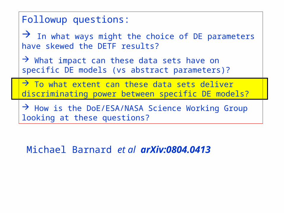
Michael Barnard et al arXiv:0804.0413
Followup questions:
In what ways might the choice of DE parameters have skewed the DETF results?
What impact can these data sets have on specific DE models (vs abstract parameters)?
To what extent can these data sets deliver discriminating power between specific DE models?
How is the DoE/ESA/NASA Science Working Group looking at these questions?

Problem:
Each scalar field model is defined in its own parameter space. How should one quantify discriminating power among models?
Our answer:
Form each set of scalar field model parameter values, map the solution into w(a) eigenmode space, the space of uncorrelated observables.
Make the comparison in the space of uncorrelated observables.

1 2 3 4 5 6 7 8 90
1
2
Stage 4 Space WL Opt; lin-a NGrid
= 9, zmax
= 4, Tag = 044301
i
0.2 0.3 0.4 0.5 0.6 0.7 0.8 0.9 1-1
0
1
f's
a
0.2 0.3 0.4 0.5 0.6 0.7 0.8 0.9 1-1
0
1
f's
a
0.2 0.3 0.4 0.5 0.6 0.7 0.8 0.9 1-1
0
1
f's
a
1
2
3
4
5
6
7
8
9
i
Prin
cipl
e A
xes
if i
a
Characterizing 9D ellipses by principle axes and corresponding errorsWL Stage 4 Opt
z-=4 z =1.5 z =0.25 z =0
1
2
Axis 1
Axis 2
1f
2f
i ii
w c f

●● ●
●
●
■■
■■
■
■ ■ ■ ■ ■
● Data■ Theory 1■ Theory 2
Concept: Uncorrelated data points (expressed in w(a) space)
0
1
2
0 5 10 15
X
Y

Starting point: MCMC chains giving distributions for each model at Stage 2.

DETF Stage 3 photo [Opt]
1 1/c
2 2/c
i ii
w c f

DETF Stage 3 photo [Opt]
1 1/c
2 2/c
i ii
w c f

DETF Stage 3 photo [Opt] Distinct model locations
mode amplitude/σi “physical”
Modes (and σi’s) reflect specific expts.
1 1/c
2 2/c

DETF Stage 3 photo [Opt]
1 1/c
2 2/c
i ii
w c f

DETF Stage 3 photo [Opt]
3 3/c
4 4/c
i ii
w c f

Eigenmodes:
Stage 3 Stage 4 gStage 4 s
z=4 z=2 z=1 z=0.5 z=0

Eigenmodes:
Stage 3 Stage 4 gStage 4 s
z=4 z=2 z=1 z=0.5 z=0
N.B. σi change too

DETF Stage 4 ground [Opt]
1 1/c
2 2/c
i ii
w c f

DETF Stage 4 ground [Opt]
3 3/c
4 4/c
i ii
w c f

DETF Stage 4 space [Opt]
1 1/c
2 2/c
i ii
w c f

DETF Stage 4 space [Opt]
3 3/c
4 4/c
i ii
w c f

0.2 0.4 0.6 0.8 1-1
-0.9
-0.8
-0.7
-0.6
-0.5
a
w(a
)
PNGBEXPITAS
The different kinds of curves correspond to different “trajectories” in mode space (similar to FT’s)
DETF Stage 4 ground
Data that reveals a universe with dark energy given by “ “ will have finite minimum “distances” to other quintessence models
powerful discrimination is possible.
2
Consider discriminating power of each experiment (look at units on axes)
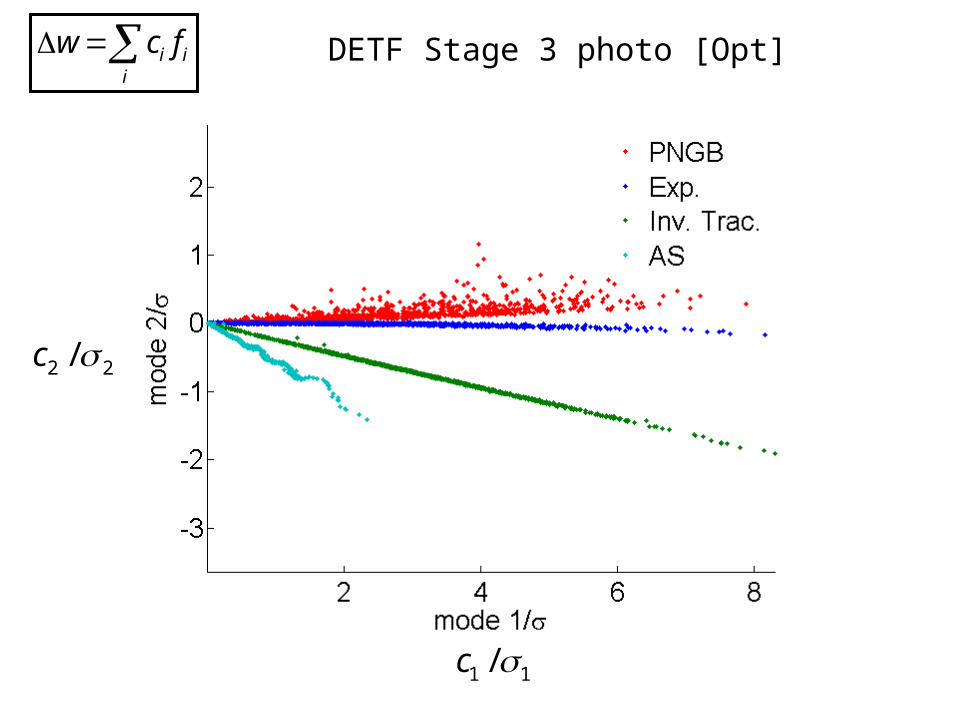
DETF Stage 3 photo [Opt]
1 1/c
2 2/c
i ii
w c f

DETF Stage 3 photo [Opt]
3 3/c
4 4/c
i ii
w c f

DETF Stage 4 ground [Opt]
1 1/c
2 2/c
i ii
w c f

DETF Stage 4 ground [Opt]
3 3/c
4 4/c
i ii
w c f
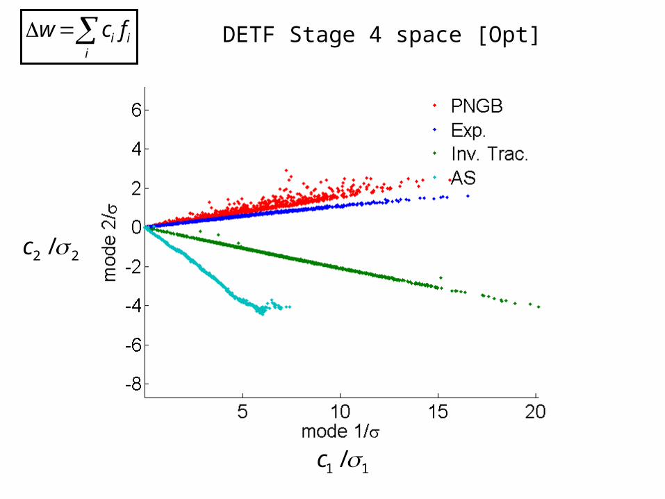
DETF Stage 4 space [Opt]
1 1/c
2 2/c
i ii
w c f
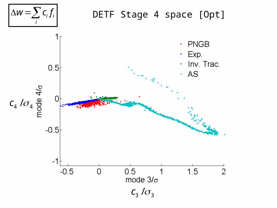
DETF Stage 4 space [Opt]
3 3/c
4 4/c
i ii
w c f

Quantify discriminating power:
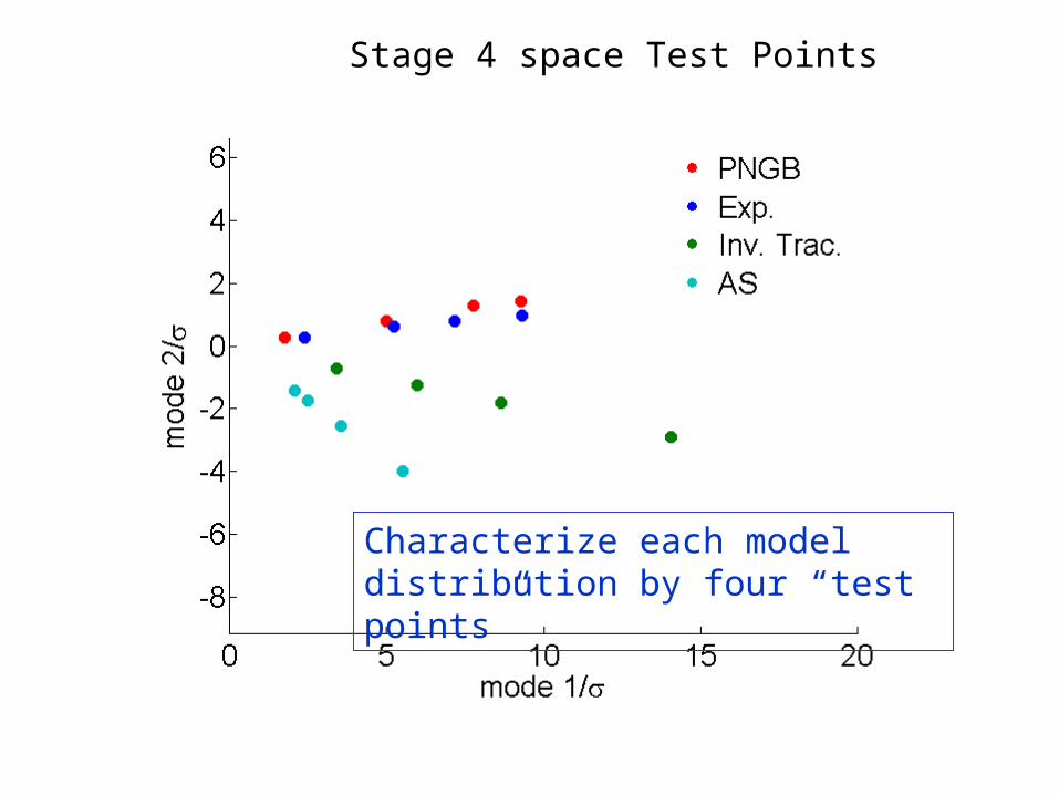
Stage 4 space Test Points
Characterize each model distribution by four “test points”

Stage 4 space Test Points
Characterize each model distribution by four “test points”
(Priors: Type 1 optimized for conservative results re discriminating power.)
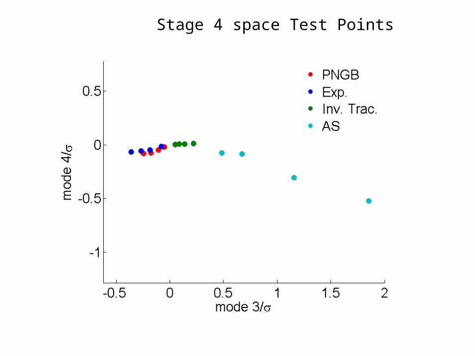
Stage 4 space Test Points

•Measured the χ2 from each one of the test points (from the “test model”) to all other chain points (in the “comparison model”).
•Only the first three modes were used in the calculation.
•Ordered said χ2‘s by value, which allows us to plot them as a function of what fraction of the points have a given value or lower.
•Looked for the smallest values for a given model to model comparison.

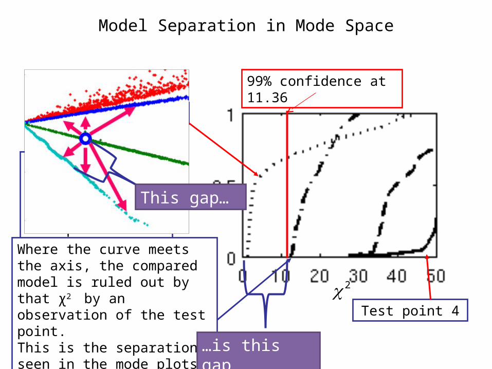
Model Separation in Mode Space
Fraction of compared model within given χ2 of test model’s test point
Test point 4
Test point 1
Where the curve meets the axis, the compared model is ruled out by that χ2 by an observation of the test point.This is the separation seen in the mode plots.
99% confidence at 11.36
2
2
Model Separation in Mode Space
Fraction of compared model within given χ2 of test model’s test point
Test point 4
Test point 1
Where the curve meets the axis, the compared model is ruled out by that χ2 by an observation of the test point.This is the separation seen in the mode plots.
99% confidence at 11.36
…is this gap
This gap…
2

DETF Stage 3 photoTe
st P
oint
Mod
elComparison Model
[4 models] X [4 models] X [4 test points]

DETF Stage 3 photoTe
st P
oint
Mod
elComparison Model

DETF Stage 4 groundTe
st P
oint
Mod
elComparison Model
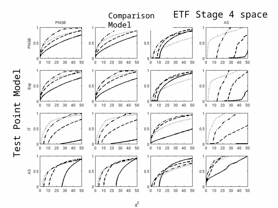
DETF Stage 4 spaceTe
st P
oint
Mod
elComparison Model

PNGB PNGB Exp IT AS
Point 1 0.001 0.001 0.1 0.2
Point 2 0.002 0.01 0.5 1.8
Point 3 0.004 0.04 1.2 6.2
Point 4 0.01 0.04 1.6 10.0
Exp
Point 1 0.004 0.001 0.1 0.4
Point 2 0.01 0.001 0.4 1.8
Point 3 0.03 0.001 0.7 4.3
Point 4 0.1 0.01 1.1 9.1
IT
Point 1 0.2 0.1 0.001 0.2
Point 2 0.5 0.4 0.0004 0.7
Point 3 1.0 0.7 0.001 3.3
Point 4 2.7 1.8 0.01 16.4
AS
Point 1 0.1 0.1 0.1 0.0001
Point 2 0.2 0.1 0.1 0.0001
Point 3 0.2 0.2 0.1 0.0002
Point 4 0.6 0.5 0.2 0.001
DETF Stage 3 photo
A tabulation of χ2 for each graph where the curve crosses the x-axis (= gap)For the three parameters used here, 95% confidence χ2 = 7.82,99% χ2 = 11.36.Light orange > 95% rejectionDark orange > 99% rejection
Blue: Ignore these because PNGB & Exp hopelessly similar, plus self-comparisons

PNGB PNGB Exp IT AS
Point 1 0.001 0.005 0.3 0.9
Point 2 0.002 0.04 2.4 7.6
Point 3 0.004 0.2 6.0 18.8
Point 4 0.01 0.2 8.0 26.5
Exp
Point 1 0.01 0.001 0.4 1.6
Point 2 0.04 0.002 2.1 7.8
Point 3 0.01 0.003 3.8 14.5
Point 4 0.03 0.01 6.0 24.4
IT
Point 1 1.1 0.9 0.002 1.2
Point 2 3.2 2.6 0.001 3.6
Point 3 6.7 5.2 0.002 8.3
Point 4 18.7 13.6 0.04 30.1
AS
Point 1 2.4 1.4 0.5 0.001
Point 2 2.3 2.1 0.8 0.001
Point 3 3.3 3.1 1.2 0.001
Point 4 7.4 7.0 2.6 0.001
DETF Stage 4 ground
A tabulation of χ2 for each graph where the curve crosses the x-axis (= gap).For the three parameters used here, 95% confidence χ2 = 7.82,99% χ2 = 11.36.Light orange > 95% rejectionDark orange > 99% rejection
Blue: Ignore these because PNGB & Exp hopelessly similar, plus self-comparisons
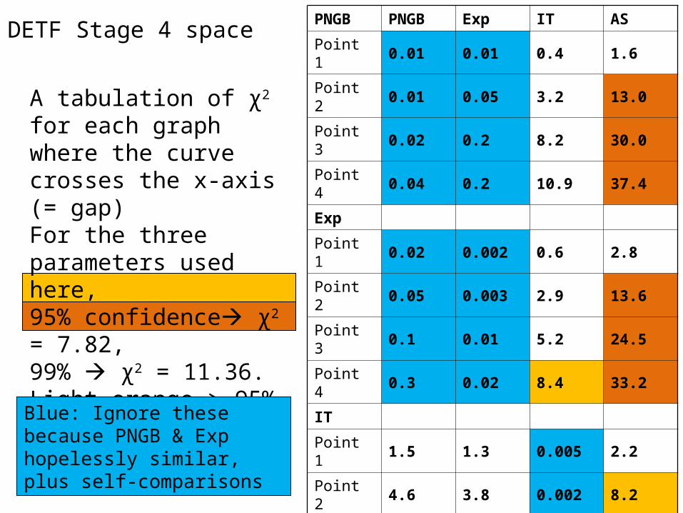
PNGB PNGB Exp IT AS
Point 1 0.01 0.01 0.4 1.6
Point 2 0.01 0.05 3.2 13.0
Point 3 0.02 0.2 8.2 30.0
Point 4 0.04 0.2 10.9 37.4
Exp
Point 1 0.02 0.002 0.6 2.8
Point 2 0.05 0.003 2.9 13.6
Point 3 0.1 0.01 5.2 24.5
Point 4 0.3 0.02 8.4 33.2
IT
Point 1 1.5 1.3 0.005 2.2
Point 2 4.6 3.8 0.002 8.2
Point 3 9.7 7.7 0.003 9.4
Point 4 27.8 20.8 0.1 57.3
AS
Point 1 3.2 3.0 1.1 0.002
Point 2 4.9 4.6 1.8 0.003
Point 3 10.9 10.4 4.3 0.01
Point 4 26.5 25.1 10.6 0.01
DETF Stage 4 space
A tabulation of χ2 for each graph where the curve crosses the x-axis (= gap)For the three parameters used here, 95% confidence χ2 = 7.82,99% χ2 = 11.36.Light orange > 95% rejectionDark orange > 99% rejection
Blue: Ignore these because PNGB & Exp hopelessly similar, plus self-comparisons
PNGB PNGB Exp IT AS
Point 1 0.01 0.01 .09 3.6
Point 2 0.01 0.1 7.3 29.1
Point 3 0.04 0.4 18.4 67.5
Point 4 0.09 0.4 24.1 84.1
Exp
Point 1 0.04 0.01 1.4 6.4
Point 2 0.1 0.01 6.6 30.7
Point 3 0.3 0.01 11.8 55.1
Point 4 0.7 0.05 18.8 74.6
IT
Point 1 3.5 2.8 0.01 4.9
Point 2 10.4 8.5 0.01 18.4
Point 3 21.9 17.4 0.01 21.1
Point 4 62.4 46.9 0.2 129.0
AS
Point 1 7.2 6.8 2.5 0.004
Point 2 10.9 10.3 4.0 0.01
Point 3 24.6 23.3 9.8 0.01
Point 4 59.7 56.6 23.9 0.01
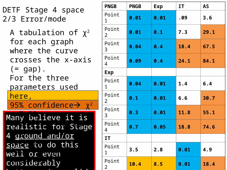
DETF Stage 4 space2/3 Error/mode
Many believe it is realistic for Stage 4 ground and/or space to do this well or even considerably better. (see slide 5)
A tabulation of χ2 for each graph where the curve crosses the x-axis (= gap).For the three parameters used here, 95% confidence χ2 = 7.82,99% χ2 = 11.36.Light orange > 95% rejectionDark orange > 99% rejection

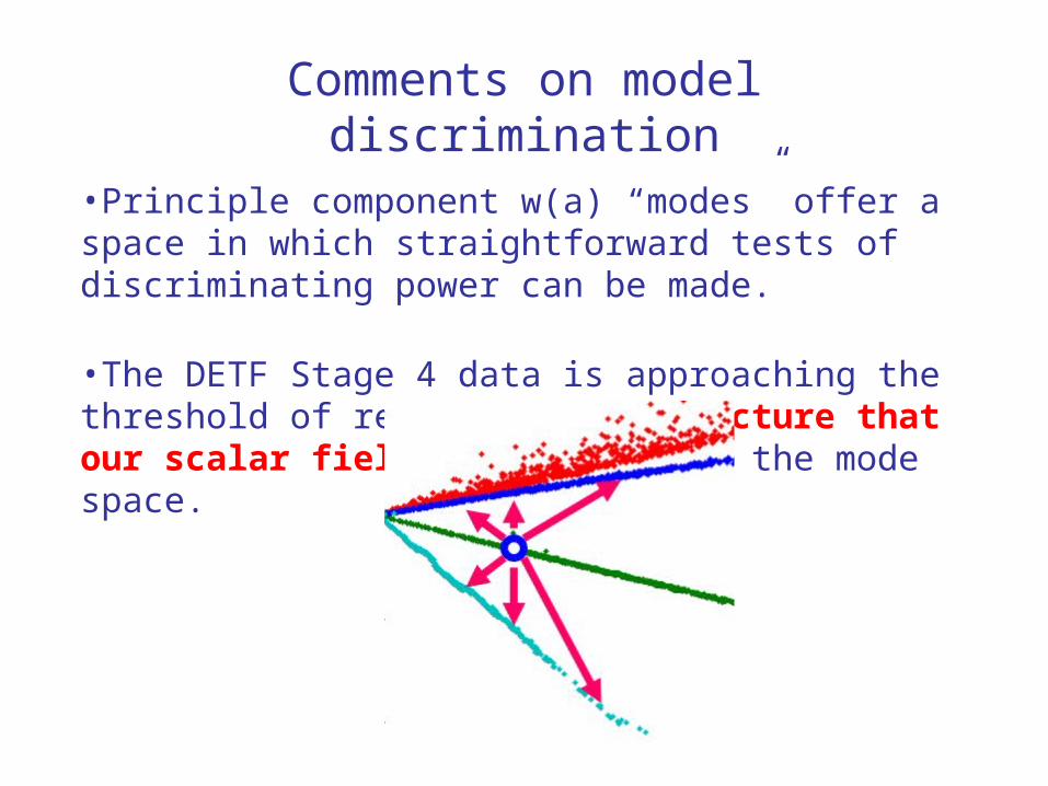
Comments on model discrimination
•Principle component w(a) “modes” offer a space in which straightforward tests of discriminating power can be made.
•The DETF Stage 4 data is approaching the threshold of resolving the structure that our scalar field models form in the mode space.

Comments on model discrimination
•Principle component w(a) “modes” offer a space in which straightforward tests of discriminating power can be made.
•The DETF Stage 4 data is approaching the threshold of resolving the structure that our scalar field models form in the mode space.
Comments on model discrimination
•Principle component w(a) “modes” offer a space in which straightforward tests of discriminating power can be made.
•The DETF Stage 4 data is approaching the threshold of resolving the structure that our scalar field models form in the mode space.

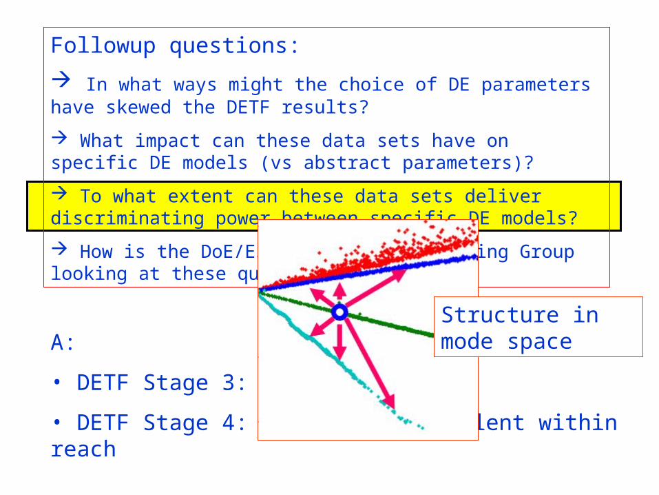
Followup questions:
In what ways might the choice of DE parameters have skewed the DETF results?
What impact can these data sets have on specific DE models (vs abstract parameters)?
To what extent can these data sets deliver discriminating power between specific DE models?
How is the DoE/ESA/NASA Science Working Group looking at these questions?
A:
• DETF Stage 3: Poor
• DETF Stage 4: Marginal… Excellent within reach
Structure in mode space

Followup questions:
In what ways might the choice of DE parameters have skewed the DETF results?
What impact can these data sets have on specific DE models (vs abstract parameters)?
To what extent can these data sets deliver discriminating power between specific DE models?
How is the DoE/ESA/NASA Science Working Group looking at these questions?
A:
• DETF Stage 3: Poor
• DETF Stage 4: Marginal… Excellent within reach

Followup questions:
In what ways might the choice of DE parameters have skewed the DETF results?
What impact can these data sets have on specific DE models (vs abstract parameters)?
To what extent can these data sets deliver discriminating power between specific DE models?
How is the DoE/ESA/NASA Science Working Group looking at these questions?

DoE/ESA/NASA JDEM Science Working Group
Update agencies on figures of merit issues
formed Summer 08
finished ~now (moving on to SCG)
Use w-eigenmodes to get more complete picture
also quantify deviations from Einstein gravity
For today: Something new we learned about (normalizing) modes

NB: in general the s form a complete basis:
D Di i
i
w c f
if
The are independently measured qualities with errors
ic
i
Define
/Di if f a
which obey continuum normalization:
D Di j ijf k f k a
then
where
i ii
w c f
Di ic c a

D Di i
i
w c f
Define
/Di if f a
which obey continuum normalization:
D Di j ijf k f k a
then
whereDi ic c a
Q: Why?
A: For lower modes, has typical grid independent “height” O(1), so one can more directly relate values of to one’s thinking (priors) on
Djf
Di i a
w
D Di i i i
i i
w c f c f

2 4 6 8 10 12 14 16 18 200
2
4
DETF= Stage 4 Space Opt All fk=6
= 1, Pr = 0
4210.50.20-2
0
2
z
Mode 1Mode 2
00.20.40.60.81-2
0
2
a
Mode 3
4210.50.20-2
0
2
z
Mode 4
i
Prin
cipl
e A
xes
(w(z
))
if
DETF Stage 4

4210.50.20-2
0
2
z
DETF= Stage 4 Space Opt All fk=6
= 1, Pr = 0
Mode 5
00.20.40.60.81-2
0
2
a
Mode 6
4210.50.20-2
0
2
z
Mode 7
4210.50.20-2
0
2
z
Mode 8
Prin
cipl
e A
xes
(w(z
))
if
DETF Stage 4

Upshot: More modes are interesting (“well measured” in a grid invariant sense) than previously thought.

0 5 10
10-3
10-2
10-1
100
101
102
mode
aver
age
proj
ectio
n
PNGB meanExp. meanIT meanAS meanPNGB maxExp. maxIT maxAS max

An example of the power of the principle component analysis:
Q: I’ve heard the claim that the DETF FoM is unfair to BAO, because w0-wa does not describe the high-z behavior to which BAO is particularly sensitive. Why does this not show up in the 9D analysis?

BAOp BAOs SNp SNs WLp ALLp1
10
100
1e3
1e4
Stage 3
Bska Blst Slst Wska Wlst Aska Alst1
10
100
1e3
1e4
Stage 4 Ground
BAO SN WL S+W S+W+B1
10
100
1e3
1e4
Stage 4 Space
Grid Linear in a zmax = 4 scale: 0
1
10
100
1e3
1e4
Stage 4 Ground+Space
[SSBlstW lst] [BSSlstW lst] Alllst [SSWSBIIIs] SsW lst
DETF(-CL)
9D (-CL)
DETF/9DF
Specific Case:

1 2 3 4 5 6 7 8 90
1
2
Stage 4 Space WL Opt; lin-a NGrid
= 9, zmax
= 4, Tag = 044301
i
0.2 0.3 0.4 0.5 0.6 0.7 0.8 0.9 1-1
0
1
f's
a
0.2 0.3 0.4 0.5 0.6 0.7 0.8 0.9 1-1
0
1
f's
a
0.2 0.3 0.4 0.5 0.6 0.7 0.8 0.9 1-1
0
1
f's
a
1
2
3
4
5
6
7
8
9
i
Prin
cipl
e A
xes
if i
a
Characterizing 9D ellipses by principle axes and corresponding errorsWL Stage 4 Opt
z-=4 z =1.5 z =0.25 z =0

1 2 3 4 5 6 7 8 90
1
2
Stage 4 Space BAO Opt; lin-a NGrid
= 9, zmax
= 4, Tag = 044301
i
0.2 0.3 0.4 0.5 0.6 0.7 0.8 0.9 1-1
0
1
f's
a
0.2 0.3 0.4 0.5 0.6 0.7 0.8 0.9 1-1
0
1
f's
a
0.2 0.3 0.4 0.5 0.6 0.7 0.8 0.9 1-1
0
1
f's
a
1
2
3
4
5
6
7
8
9
BAO
z-=4 z =1.5 z =0.25 z =0
1 2 3 4 5 6 7 8 90
1
2
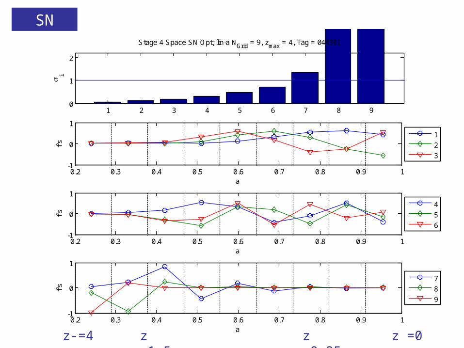
Stage 4 Space SN Opt; lin-a NGrid
= 9, zmax
= 4, Tag = 044301
i
0.2 0.3 0.4 0.5 0.6 0.7 0.8 0.9 1-1
0
1
f's
a
0.2 0.3 0.4 0.5 0.6 0.7 0.8 0.9 1-1
0
1
f's
a
0.2 0.3 0.4 0.5 0.6 0.7 0.8 0.9 1-1
0
1
f's
a
1
2
3
4
5
6
7
8
9
SN
z-=4 z =1.5 z =0.25 z =0

1 2 3 4 5 6 7 8 90
1
2
Stage 4 Space BAO Opt; lin-a NGrid
= 9, zmax
= 4, Tag = 044301
i
0.2 0.3 0.4 0.5 0.6 0.7 0.8 0.9 1-1
0
1
f's
a
0.2 0.3 0.4 0.5 0.6 0.7 0.8 0.9 1-1
0
1
f's
a
0.2 0.3 0.4 0.5 0.6 0.7 0.8 0.9 1-1
0
1
f's
a
1
2
3
4
5
6
7
8
9
BAODETF 1 2,
z-=4 z =1.5 z =0.25 z =0

SN
1 2 3 4 5 6 7 8 90
1
2
Stage 4 Space SN Opt; lin-a NGrid
= 9, zmax
= 4, Tag = 044301
i
0.2 0.3 0.4 0.5 0.6 0.7 0.8 0.9 1-1
0
1
f's
a
0.2 0.3 0.4 0.5 0.6 0.7 0.8 0.9 1-1
0
1
f's
a
0.2 0.3 0.4 0.5 0.6 0.7 0.8 0.9 1-1
0
1
f's
a
1
2
3
4
5
6
7
8
9
DETF 1 2,
z-=4 z =1.5 z =0.25 z =0
1 2 3 4 5 6 7 8 90
1
2
Stage 4 Space SN Opt; lin-a NGrid
= 9, zmax
= 4, Tag = 044301
i
0.2 0.3 0.4 0.5 0.6 0.7 0.8 0.9 1-1
0
1
f's
a
0.2 0.3 0.4 0.5 0.6 0.7 0.8 0.9 1-1
0
1
f's
a
0.2 0.3 0.4 0.5 0.6 0.7 0.8 0.9 1-1
0
1
f's
a
1
2
3
4
5
6
7
8
9
z-=4 z =1.5 z =0.25 z =0
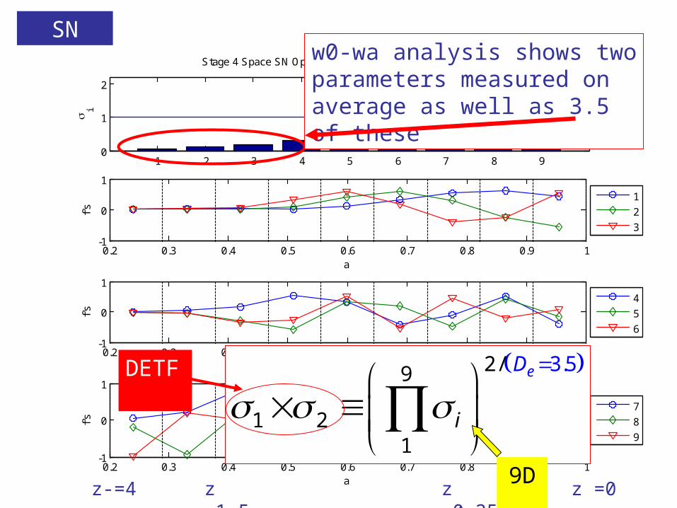
SNw0-wa analysis shows two parameters measured on average as well as 3.5 of these
2/9
1 21
3.5eD
i
DETF
9D

Stage 2

Stage 2
Stage 2

Stage 2

Stage 2

Stage 2

Stage 2
Detail: Model discriminating power
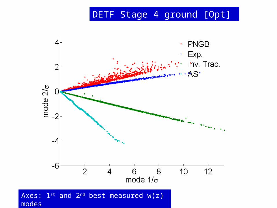
DETF Stage 4 ground [Opt]
Axes: 1st and 2nd best measured w(z) modes

DETF Stage 4 ground [Opt] DETF Stage 4 ground [Opt]
Axes: 3rd and 4th best measured w(z) modes


