Dark Matter Dynamics by Phillip Gregory Zukin B.S. Physics California Institute of Technology (2006) Submitted to the Department of Physics in partial fulfillment of the requirements for the degree of Doctor of Philosophy in Physics at the MASSACHUSETTS INSTITUTE OF TECHNOLOGY May 2012 c Phillip Gregory Zukin, MMXII. All rights reserved. The author hereby grants to MIT permission to reproduce and to distribute publicly paper and electronic copies of this thesis document in whole or in part in any medium now known or hereafter created. Author .............................................................. Department of Physics May 18, 2012 Certified by .......................................................... Edmund Bertschinger Department Head, Professor of Physics Thesis Supervisor Accepted by ......................................................... Krishna Rajagopal Professor of Physics Associate Department Head for Education
Transcript
Dark Matter Dynamics
by
Phillip Gregory Zukin
B.S. PhysicsCalifornia Institute of Technology (2006)
Submitted to the Department of Physicsin partial fulfillment of the requirements for the degree of
Submitted to the Department of Physicson May 18, 2012, in partial fulfillment of the
requirements for the degree ofDoctor of Philosophy in Physics
Abstract
N-body simulations have revealed a wealth of information about dark matter halosbut their results are largely empirical. Here we attempt to shed light on simulationresults by using a combination of analytic and numerical methods. First we gener-alize an analytic model of halo formation, known as Secondary Infall, to include theeffects of tidal torque. Given this model we compare its predictions for halo profilesto simulation results and infer that angular momentum plays an important role insetting the structure of dark matter profiles at small radii. Next, we focus on explain-ing the origin of universality in halos. We find evidence that diffusion – which canpotentially lead to universality – occurs during halo evolution and is partially sourcedby external torques from large scale structure. This is surprising given that the halois nonlinear and typically thought to be unaffected by neighboring structures. Last,we describe promising ways to analytically describe the evolution of nonlinear halosusing a Fokker-Planck formalism.
Thesis Supervisor: Edmund BertschingerTitle: Department Head, Professor of Physics
3
4
Acknowledgments
Thank you to my advisor, Ed Bertschinger, for his guidance. Thank you to the
Astrophysics Department and the MKI community for their enthusiasm and passion
for this field, which fueled my own. Thank you to my family for their love and
support.
5
6
For my grandparents
8
Contents
1 Introduction 15
2 Self-Similar Spherical Collapse with Tidal Torque 21
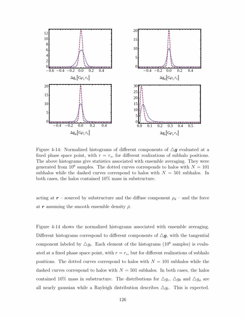
4-14 Histograms showing the effects of ensemble averaging . . . . . . . . . 126
4-15 Histograms showing the effects of phase space averaging . . . . . . . . 128
4-16 Histograms showing the effects of time averaging . . . . . . . . . . . . 129
14
Chapter 1
Introduction
The energy content of the universe, through Einstein’s theory of General Relativ-
ity, influences the universe’s geometry and evolution. Therefore – assuming General
Relativity is correct – we can constrain the universe’s components by measuring the
geometry of the universe at different times. To measure the geometry of the universe,
cosmologists use what is known as standard candles and standard rulers. These are as-
tronomical objects for which we know their intrinsic brightness or size, respectively.
Knowing the intrinsic brightness or size of an object, and measuring the object’s
apparent brightness or apparent size, constrains the distance to that object. This
distance, when coupled with General Relativity, then allows us to infer the contents
of the universe.
One common standard candle is a Supernovae Type IA explosion, which is believed
to occur when a White Dwarf accretes enough matter from a neighboring star to
become unstable, and then detonates. These extremely luminous explosions are ob-
servable very far away. Interestingly, they appear dimmer than cosmologists would
have initially expected, leading the community to believe that the universe is currently
undergoing an epoch of cosmological acceleration (Riess et al., 1998; Perlmutter et al.,
1999). This is very unintuitive. Given an initial Big Bang, one would expect gravity
acting on matter to pull back and decelerate the expansion of the universe. However,
this observation implies that the universe is composed of a material that forces gravity
15
to push out and accelerate the expansion. The material that sources this expansion is
called dark energy; the scientists who made the observations leading to dark energy’s
discovery have recently been awarded the Nobel Prize.
Supernovae explosions test our understanding of the universe on large scales and re-
veal that dark energy is a major component of our universe. It is also possible to
test our understanding of the universe on smaller scales – like that of a galaxy – by
calculating the mass of galaxies using two independent methods and then comparing
both mass estimates. One method is dynamical in nature. Astronomers estimate the
mass – assuming Newtonian Gravity is valid on these scales – based on the speed of
orbiting objects. The other method is photometric in nature. Astronomers observe a
total amount of light coming from the galaxy. They assume the galaxy is composed
of stars. Given the mass and luminosity of an individual star, they then convert some
total observed luminosity of the galaxy to an estimate of the total mass. With these
two independent estimates of the mass, astronomers found that the dynamical mass
estimate is much larger than the photometric estimate (Rubin & Ford, 1970). This,
assuming Newton correctly described gravity on these scales, implies that there is a
significant amount of mass in a galaxy that is not visible. This invisible component
is known as Dark Matter; its existence was postulated by Zwicky in the 1930s based
on observations of the Coma Cluster.
Observations like those described above – on both cosmological and galaxy scales
– coupled with General Relativity, constrain our universe today to be composed of
roughly 73% dark energy, 23% dark matter and 4% baryons (Komatsu et al., 2010).
While baryons are directly observable and well understood, dark energy and dark
matter are complete mysteries.
The simplest models for dark energy assume that it does not cluster. In other words,
gravity does not produce dark energy clumps. Dark matter, on the other hand, can
cluster. Therefore, as the universe evolves, dark energy stays smooth throughout,
16
while the dark matter gets more and more concentrated as gravity pulls matter onto
initial over-densities. These large concentrations of dark matter are where galaxies
eventually form.
Galaxy formation is a complicated nonlinear process. Our current understanding is
that gravity makes dark matter clumps that grow with time. Initially, the baryons
and dark matter are evenly mixed. Over time, however, since baryons can lose energy
through more pathways than dark matter, most baryons settle into the center of the
clumps. While at early times only gravity is relevant, other forces become important
later on as baryons start to radiatively and mechanically couple to their environment.
Galaxy formation is of great interest to the community. Comparing theoretically
predicted galaxies to observed ones not only tests our cosmological model on large
scales, it also tests our theoretical understanding of astrophysical processes within
galaxies. In other words, galaxies are systems which allow us to test our under-
standing of physics over a wide range of scales. Given the complex nature of galaxy
formation – with many competing processes – it is best to first focus on the most
massive component of a galaxy, known as the dark matter halo. Doing so simplifies
the problem. Then – given a fundamental understanding of halo formation – one
can later add complications in order to take into account the influence of baryons
and develop a model which matches observations of galaxies. This thesis, as a result,
focuses exclusively on dark matter halo formation.
A dark matter halo is composed of many gravitationally interacting dark matter par-
ticles. If a system contains more than two gravitationally interacting particles, it
becomes difficult to understand completely with pen and paper. As a result, most
studies of halo formation use purely numerical methods and run large computer pro-
grams known as N-body simulations. While numerical methods are useful, in order
to really understand how halos form, it is necessary to develop analytic models that
explain and bring intuition to the numerical results.
17
There is currently a large community of theoretical cosmologists that work on N-
body simulations. Initially, the particles are given positions and velocities that are
consistent with linear perturbation theory. These initial conditions are only valid at
very early times before the dark matter starts to clump significantly. Then particles
are evolved forward in time only subject to gravitational forces. Today, simulated
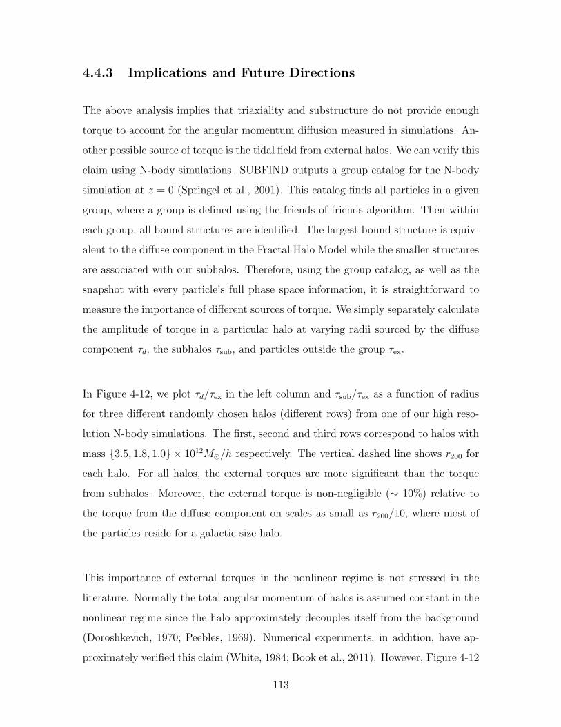
universes shows distinct groups of particles – dark matter halos – of varying size
ranging from roughly 106M⊙ to 1014M⊙. The lower limit depends on the mass of the
smallest particle in the simulation while the upper limit depends on the size of the
cosmological box simulated.
Many interesting trends have been discovered with these simulations. First, the den-
sity profiles of all halos can roughly be fit by an empirical formula, known as the
NFW profile, that only depends on two parameters (Navarro et al., 1996, 1997). In
addition, the pseudo-phase space density, which depends on the velocity of particles
in the halo, also seems to follow a single functional form – the same power law –
in different halos (Taylor & Navarro, 2001; Ludlow et al., 2010). Naively one would
expect these quantities to depend on initial conditions, environment, and mass of
the halo. However, N-body simulations find that – aside from scalings – the density
and pseudo-phase space density profiles of halos are universal. This universality is
extremely surprising and immediately brings forth many interesting theoretical ques-
tions. What is the origin of the NFW profile? Are dynamical processes responsible
for the universality of these profiles? Why are certain halo properties universal while
others are not?
While all of these dark matter halo properties are informative, they are all empirical.
In order to gain better intuition for halo formation – and eventually galaxy forma-
tion – and understand the origin of these empirical relationships, this thesis explores
different ways to analytically model halo formation.
18
Understanding halos analytically is straightforward at early times. Halos are initially
linear in the quantity δ ≡ (ρ− ρ)/ρ, where ρ is the density and ρ is the mean matter
density in the universe. For δ ≪ 1, the dark matter fluid equations of motion can
be linearized and it is found that the over-density grows with time – in the matter
dominated era – according to δ ∝ t2/3 where t is the age of the universe. At one point,
as the universe evolves, the over-density becomes δ ∼ 1 and the fluid equations are
no longer valid. Hence it is necessary to explore other analytic techniques in order to
track a halo’s evolution into the nonlinear regime where we typically observe halos
with δ > 200 today.
An analytic formalism that can track a halo from the linear through the nonlinear
regime is known as the Self-Similar Secondary Infall model (Gunn & Gott, 1972;
Gott, 1975; Gunn, 1977). Secondary Infall describes the continuous accretion of mass
shells onto an initial over-density. Self-similarity constrains the system to look iden-
tical when scaled in time and amplitude. Moreover, imposing self-similarity makes
the system analytically tractable. In this thesis we generalize the model to take into
account tidal torques acting on particles within the halo. In Chapters 2 and 3, we
use our generalized model to gain intuition about the density and velocity profiles of
dark matter halos. Both chapters are heavily based on published papers (Zukin &
Bertschinger, 2010a,b).
In Chapter 4, we explore the origin of the ‘observed’ universality. Universality implies
that information in the system has been lost, since the result does not depend on initial
conditions, mass, or environment. One way to lose information is through dynamical
processes, like diffusion. Another way occurs when analyzing the data, where for
instance all angular informative is averaged over when calculating a radial density
profile. In Chapter 4 we analyze the roles each of these mechanisms play in causing
universality by using a combination of numerical and analytic methods.
19
20
Chapter 2
Self-Similar Spherical Collapse
with Tidal Torque 1
Abstract
N-body simulations have revealed a wealth of information about dark matter haloshowever their results are largely empirical. Using analytic means, we attempt to shedlight on simulation results by generalizing the self-similar secondary infall model toinclude tidal torque. In this chapter, we describe our halo formation model and com-pare our results to empirical mass profiles inspired by N-body simulations. Each halois determined by four parameters. One parameter sets the mass scale and the otherthree define how particles within a mass shell are torqued throughout evolution. Wechoose torque parameters motivated by tidal torque theory and N-body simulationsand analytically calculate the structure of the halo in different radial regimes. We findthat angular momentum plays an important role in determining the density profileat small radii. For cosmological initial conditions, the density profile on small scalesis set by the time rate of change of the angular momentum of particles as well as thehalo mass. On intermediate scales, however, ρ ∝ r−2, while ρ ∝ r−3 close to the virialradius.
2.1 Introduction
The structure of dark matter halos affects our understanding of galaxy formation
and evolution and has implications for dark matter detection. Progress in our un-
derstanding of dark matter halos has been made both numerically and analytically.
1This chapter is based on the published paper Zukin & Bertschinger 2010a
21
Analytic treatments began with work by Gunn and Gott; they analyzed how bound
mass shells that accrete onto an initially collapsed object can explain the morphology
of the Coma cluster (Gunn & Gott, 1972; Gott, 1975) and elliptical galaxies (Gunn,
1977). This continuous accretion process is known as secondary infall.
Secondary infall introduces a characteristic length scale: the shell’s turnaround
radius r∗. This is the radius at which a particular mass shell first turns around. Since
the average density is a decreasing function of distance from the collapsed object, mass
shells initially farther away will turnaround later. This characteristic scale should be
expected since the radius of a mass shell, like the radius of a shock wave in the Sedov
Taylor solution, can only depend on the initial energy of the shell, the background
density, and time (Bertschinger, 1985). By imposing that the structure of the halo
is self-similar – all quantities describing the halo only depend on the background
density, rta (the current turnaround radius), and lengths scaled to rta – Bertschinger
(1985), and Fillmore & Goldreich (1984), (hereafter referred to as FG) were able to
relate the asymptotic slope of the nonlinear density profile to the initial linear density
perturbation.
Assuming purely radial orbits, FG analytically showed that the slope ν of the
halo density distribution ρ ∝ r−ν falls in the range 2 < ν < 2.25 for r/rta ≪ 1.
This deviates strongly from N-body simulations which find ν ∼< 1 (Navarro et al.,
2010; Graham et al., 2006) or ν ∼ 1.2 (Diemand et al., 2004) at their innermost
resolved radius and observations of Low Surface Brightness and spiral galaxies which
suggest ν ∼ .2 (de Blok, 2003) and the presence of cores (Gentile et al., 2004; Salucci
et al., 2007; Donato et al., 2009). Though the treatment in FG assumes radial orbits
while orbits in simulations and observed galaxies contain tangential components, it
is analytically tractable and does not suffer from resolution limits. Numerical dark
matter simulations, on the other hand, do not make any simplifying assumptions
and have finite dynamic range. Moreover, it is difficult to draw understanding from
their analysis and computational resources limit the smallest resolvable radius, since
smaller scales require more particles and smaller time steps. It seems natural, then,
to generalize the work done by FG in order to explain the features predicted in
22
simulations and observed in galaxies. This chapter, in particular, investigates how
non-radial motion affects the structure of dark matter halos.
Numerous authors have investigated how angular momentum affects the asymp-
totic density profile. Ryden & Gunn (1987) analyzed the effects of non-radial motion
caused by substructure while others have examined how an angular momentum, or a
distribution of angular momenta, assigned to each mass shell at turnaround, affects
the structure of the halo (Nusser, 2001; Hiotelis, 2002; Williams et al., 2004; Sikivie
et al., 1997; Del Popolo, 2009; White & Zaritsky, 1992; Le Delliou & Henriksen,
2003; Ascasibar et al., 2004). Note that many of these authors do not impose self-
similarity. Those that do assume that a shell’s angular momentum remains constant
after turnaround.
This chapter extends previous work by Nusser (2001). Assuming self-similarity,
he analytically calculated the structure of the halo in different radial regimes for
shells with constant angular momentum after turnaround. He found that the inclu-
sion of angular momentum allows 0 < ν < 2.25. According to Hoffman & Shaham
(1985), ν depends on the effective primordial power spectral index (d lnP/d ln k),
which varies for different mass halos. For galactic size halos, Nusser’s analytic work
predicts ν ∼ 1.3, in disagreement with simulation results (Navarro et al., 2010; Die-
mand et al., 2004). In order to address this discrepancy, we extend Nusser’s work
by including torque. We consistently keep track of a particle’s angular momentum,
allowing it to build up before turnaround because of tidal interactions with neighbor-
ing protogalaxies (Hoyle, 1951) and to evolve after turnaround because of nonlinear
effects within the halo. Moreover, we compare the predictions of our halo model to
simulation results.
Self-similar secondary infall requires Ωm = 1 since a nonvanishing ΩΛ introduces
an additional scale. Applying self-similarity to halo formation in the ΛCDM model
therefore requires approximations and a mapping to halos in an Einstein de-Sitter
universe. We assume that the linear power spectrum and background matter density
ρm today are equal in both universes so that the statistics, masses, and length scales of
halos found in the two models are equivalent. Since the scale factor evolves differently
23
in both universes, the halo assembly histories will differ.
In section 2.2, we define our self-similar system and torqueing parameters. In
section 2.3, we set initial conditions and evolve the mass shells before turnaround. In
section 2.4, we describe evolution after turnaround and then analyze the asymptotic
behavior of the density profile at different scales in section 2.5. In section 2.6, we give
numerical results, discuss the overall structure of the halo, and compare to N-body
simulations. We conclude in section 2.7.
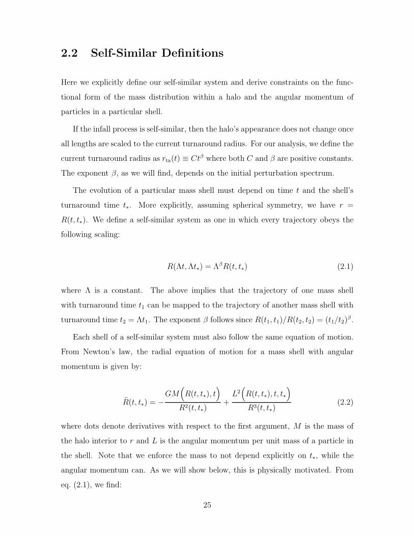
This chapter requires the use of many equations and symbols. As a guide to the
reader, in Table 2.1 we summarize the key symbols and the equations where they are
defined or first used.
Table 2.1: Symbols Used in this Chapter
Symbol Meaning Reference Equation
r∗ Turnaround radius of an individual shell ...t∗ Turnaround time of an individual shell ...rta Current turnaround radius ...L Angular momentum per unit mass (2.8)δ Initial density perturbation ...β Exponent characterizing rta (2.20)n Exponent characterizing δ (2.17)p Exponent characterizing correction to δ caused by L (2.17)B Amplitude of L at turnaround (2.8), (2.30)γ Exponent characterizing evolution of L (t < t∗) (2.12) Exponent characterizing evolution of L (t > t∗) (2.12)λ Radius scaled to current turnaround radius ...f Angular momentum normalized by self-similar scaling (2.8), (2.12)D Density normalized by self-similar scaling (2.9)M Internal mass normalized by self-similar scaling (2.10)ξ Time variable: ln(t/tta) ...ra Apocenter distance of an individual shell ...rp Pericenter distance of an individual shell ...y Ratio of pericenter to apocenter distance (2.41)y0 Proportional to first pericenter at turnaround (rp/r∗) ...α Exponent characterizing slope of nonlinear internal mass (2.37)q Exponent characterizing evolution of apocenter distance (2.38)l Exponent characterizing evolution of y (2.44)
24
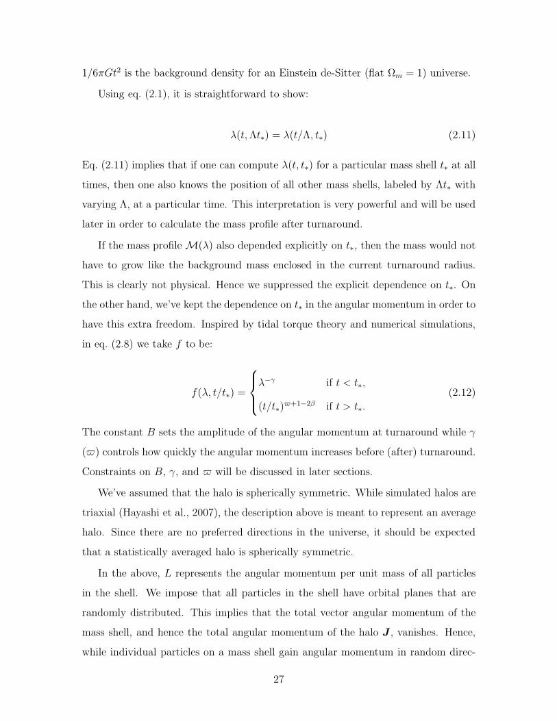
2.2 Self-Similar Definitions
Here we explicitly define our self-similar system and derive constraints on the func-
tional form of the mass distribution within a halo and the angular momentum of
particles in a particular shell.
If the infall process is self-similar, then the halo’s appearance does not change once
all lengths are scaled to the current turnaround radius. For our analysis, we define the
current turnaround radius as rta(t) ≡ Ctβ where both C and β are positive constants.
The exponent β, as we will find, depends on the initial perturbation spectrum.
The evolution of a particular mass shell must depend on time t and the shell’s
turnaround time t∗. More explicitly, assuming spherical symmetry, we have r =
R(t, t∗). We define a self-similar system as one in which every trajectory obeys the
following scaling:
R(Λt,Λt∗) = ΛβR(t, t∗) (2.1)
where Λ is a constant. The above implies that the trajectory of one mass shell
with turnaround time t1 can be mapped to the trajectory of another mass shell with
turnaround time t2 = Λt1. The exponent β follows since R(t1, t1)/R(t2, t2) = (t1/t2)β.
Each shell of a self-similar system must also follow the same equation of motion.
From Newton’s law, the radial equation of motion for a mass shell with angular
momentum is given by:
R(t, t∗) = −GM
(
R(t, t∗), t)
R2(t, t∗)+L2(
R(t, t∗), t, t∗
)
R3(t, t∗)(2.2)
where dots denote derivatives with respect to the first argument, M is the mass of
the halo interior to r and L is the angular momentum per unit mass of a particle in
the shell. Note that we enforce the mass to not depend explicitly on t∗, while the
angular momentum can. As we will show below, this is physically motivated. From
eq. (2.1), we find:
25
R(Λt,Λt∗) = Λβ−2R(t, t∗) (2.3)
Plugging in eqs. (2.1) and (2.3) into eq. (2.2) and simplifying, we find:
R(Λt,Λt∗) = − Λ3β−2GM
(
Λ−βR(Λt,Λt∗), t)
R2(Λt,Λt∗)+ Λ4β−2
L2(
Λ−βR(Λt,Λt∗), t, t∗
)
R3(Λt,Λt∗)
(2.4)
Changing variables from R(t, t∗) to R(t, t∗)/Ctβ for the mass and angular momentum
and rewriting eq. (2.4), we find:
R(Λt,Λt∗) = −Λ3β−2GM
(
R(Λt,Λt∗)/C(Λt)β, t)
R2(Λt,Λt∗)+Λ4β−2
L2(
R(Λt,Λt∗)/C(Λt)β, t, t∗
)
R3(Λt,Λt∗)(2.5)
Relabeling coordinates and enforcing consistency with eq. (2.2), we find the following
constraints on the functional forms of the mass and angular momentum.
M(
R(t, t∗)/Ctβ, t)
= Λ3β−2M(
R(t, t∗)/Ctβ, t/Λ
)
(2.6)
L(
R(t, t∗), t, t∗
)
= Λ2β−1L(
R(t, t∗)/Ctβ, t/Λ, t∗/Λ
)
(2.7)
With the above in mind, we define the angular momentum per unit mass L of a
particle in a shell at r, and the density ρ and mass M of the halo as follows.
L(r, t) = Br2ta(t)
tf(λ, t/t∗) (2.8)
ρ(r, t) = ρB(t)D(λ) (2.9)
M(r, t) =4π
3ρB(t)r
3ta(t)M(λ) (2.10)
where λ ≡ r/rta(t) is the radius scaled to the current turnaround radius and ρB =
26
1/6πGt2 is the background density for an Einstein de-Sitter (flat Ωm = 1) universe.
Using eq. (2.1), it is straightforward to show:
λ(t,Λt∗) = λ(t/Λ, t∗) (2.11)
Eq. (2.11) implies that if one can compute λ(t, t∗) for a particular mass shell t∗ at all
times, then one also knows the position of all other mass shells, labeled by Λt∗ with
varying Λ, at a particular time. This interpretation is very powerful and will be used
later in order to calculate the mass profile after turnaround.
If the mass profile M(λ) also depended explicitly on t∗, then the mass would not
have to grow like the background mass enclosed in the current turnaround radius.
This is clearly not physical. Hence we suppressed the explicit dependence on t∗. On
the other hand, we’ve kept the dependence on t∗ in the angular momentum in order to
have this extra freedom. Inspired by tidal torque theory and numerical simulations,
in eq. (2.8) we take f to be:
f(λ, t/t∗) =
λ−γ if t < t∗,
(t/t∗)+1−2β if t > t∗.
(2.12)
The constant B sets the amplitude of the angular momentum at turnaround while γ
() controls how quickly the angular momentum increases before (after) turnaround.
Constraints on B, γ, and will be discussed in later sections.
We’ve assumed that the halo is spherically symmetric. While simulated halos are
triaxial (Hayashi et al., 2007), the description above is meant to represent an average
halo. Since there are no preferred directions in the universe, it should be expected
that a statistically averaged halo is spherically symmetric.
In the above, L represents the angular momentum per unit mass of all particles
in the shell. We impose that all particles in the shell have orbital planes that are
randomly distributed. This implies that the total vector angular momentum of the
mass shell, and hence the total angular momentum of the halo J , vanishes. Hence,
while individual particles on a mass shell gain angular momentum in random direc-
27
tions throughout evolution, on average the mass shell remains spherical. Therefore,
like we’ve assumed above, only one radial equation of motion is necessary to describe
the evolution of the shell.
Since our statistically averaged halo has a vanishing total angular momentum, this
model cannot address the nonzero spin parameters observed in individually simulated
halos (Barnes & Efstathiou, 1987; Boylan-Kolchin et al., 2010). Nor can it reproduce
the nonzero value of 〈J2〉 expected from cosmological perturbation theory (Peebles,
1969; White, 1984; Doroshkevich, 1970). However,∫
L2dm where dm is the mass of
a shell, does not vanish for this model. We will use this quantity, which is a measure
of the tangential dispersion in the halo, to constrain our torque parameters.
2.3 Before Turnaround
The trajectory of the mass shell after turnaround determines the halo mass profile.
In order to start integrating at turnaround, however, the enclosed mass of the halo
must be known. For the case of purely radial orbits, the enclosed mass at turnaround
can be analytically calculated (Bertschinger, 1985; Fillmore & Goldreich, 1984). For
the case of orbits that have a time varying angular momentum, we must numerically
evolve both the trajectory and M(λ) before turnaround in order to determine the
enclosed mass at turnaround.
The trajectory of a mass shell follows from Newton’s law. We have:
d2r
dt2= −GM(r, t)
r2+L2(r, t)
r3(2.13)
Rewriting eq. (2.13) in terms of λ and ξ ≡ log(t/ti), where ti is the initial time, and
plugging in eqs. (2.8), (2.10) and (2.12), we find:
d2λ
dξ2+ (2β − 1)
dλ
dξ+ β(β − 1)λ = −2
9
M(λ)
λ2+B2λ−2γ−3 (2.14)
The angular momentum before turnaround was chosen so that eq. (2.14) does not
explicitly depend on ξ. This allows for a cleaner perturbative analysis. Since r is
28
an approximate power law in t at early times, we still have the freedom to choose a
particular torque model inspired by tidal torque theory. This will be discussed at the
end of this section.
In order to numerically solve the above equation, one must know M(λ), a function
we do not have a priori. Before turnaround, however, the enclosed mass of a particular
shell remains constant throughout evolution since no shells cross. Taking advantage
of this, we relate dr/dt to M by taking a total derivative of eq. (2.10). We find:
(
dr
dt
)
M
= βr
t− (3β − 2)Ctβ−1 M
M′(2.15)
In the above, a prime represents a derivative taken with respect to λ. Taking another
derivative of the above with respect to time, plugging into eq. (2.13) and simplifying,
we find an evolution equation for M:
β(β − 1)λ+ (3β − 2)(β − 1)MM′
− (3β − 2)2M2M′′
(M′)3= −2
9
Mλ2
+B2λ−2γ−3
(2.16)
Given eqns. (2.14) and (2.16), we must now specify initial conditions when λ≫ 1.
We assume the following perturbative solutions forD(λ) and λ(ξ) valid at early times.
M(λ) follows from eq. (2.10).
D(λ) = 1 + δ1λ−n + δ2λ
−p + ... (2.17)
M(λ) = λ3(
1 +3δ13− n
λ−n +3δ23− p
λ−p + ...
)
(2.18)
λ(ξ) = λ0e(2/3−β)ξ(1 + λ1e
α1ξ + λ2eα2ξ + ...) (2.19)
In the above, n characterizes the first order correction to the background density. It
is related to the FG parameter ǫ through n = 3ǫ. It is also related to the effective
power spectral index neff = d lnP/d ln k through n = neff + 3 (Hoffman & Shaham,
1985). Since neff depends on scale and hence halo mass (Appendix A.1), we have
29
8 9 10 11 12 13 14 15
0.6
0.8
1.0
1.2
1.4
log10HMML
n
Figure 2-1: The variation of model parameter n with halo mass. Larger mass halosmap to steeper initial density profiles.
a relationship between n and halo mass. As Figure 2-1 shows, larger mass halos
have larger n. This is expected since larger smoothing lengths imply steeper initial
density profiles. As in FG, we restrict 0 < n < 3 so that the density decreases with
radius while the mass increases. We examine this whole range for completeness even
though n > 1.4 corresponds to objects larger than galaxy clusters. The exponent p
characterizes the next order correction to the background density caused by angular
momentum. Consistency with our perturbative expansion (eqs. 2.17 through 2.19)
demands that we take n < p < 2n. However, it is straightforward to generalize to
other cases (Section 2.3.1). As we show below, the constants δ2, λ1, λ2, α1, α2 are set
by the equations of motion. The constants δ1, λ0 are set by boundary conditions.
Plugging eq. (2.18) into eq. (2.16) and enforcing equality between terms proportional
to λ1−n we find two possible solutions.
30
β =2
3
(
1 +1
n
)
(2.20)
β =2
3
(
1− 3
2n
)
(2.21)
These represent the two solutions to the second order differential equation (eq. 2.16).
For the first case, the turnaround radius grows faster than the Hubble flow while for
the second it grows slower. Hence, the first solution represents the growing mode
of the perturbation while the second is the decaying mode. Since we are interested
in the growth of halos, we will only consider the growing mode from now on. Next,
imposing p = 2γ + 4 and enforcing equality between terms proportional to λ1−p in
eq. (2.16), we find:
δ2 =9n2B2(p− 3)
2(p− n)(3n+ 2p)(2.22)
Comparing eqs. (2.18) and (2.22), we see that the correction to the initial mass caused
by angular momentum is negative since p > n. This is expected since the angular
momentum acts against gravity.
Next, we find constraints for the parameters in eq. (2.19). Plugging in eq. (2.19)
into eq. (2.14) and setting terms linear in δ1, δ2, λ1, and λ2 equal to each other, we
find:
α1 =2
3(2.23)
λ1 =δ1
n− 3λ−n0 (2.24)
α2 = p
(
β − 2
3
)
(2.25)
λ2 =δ2
p− 3λ−p0 (2.26)
Eqns. (2.17) through (2.26) set the initial conditions for eqs (2.14) and (2.16). We
31
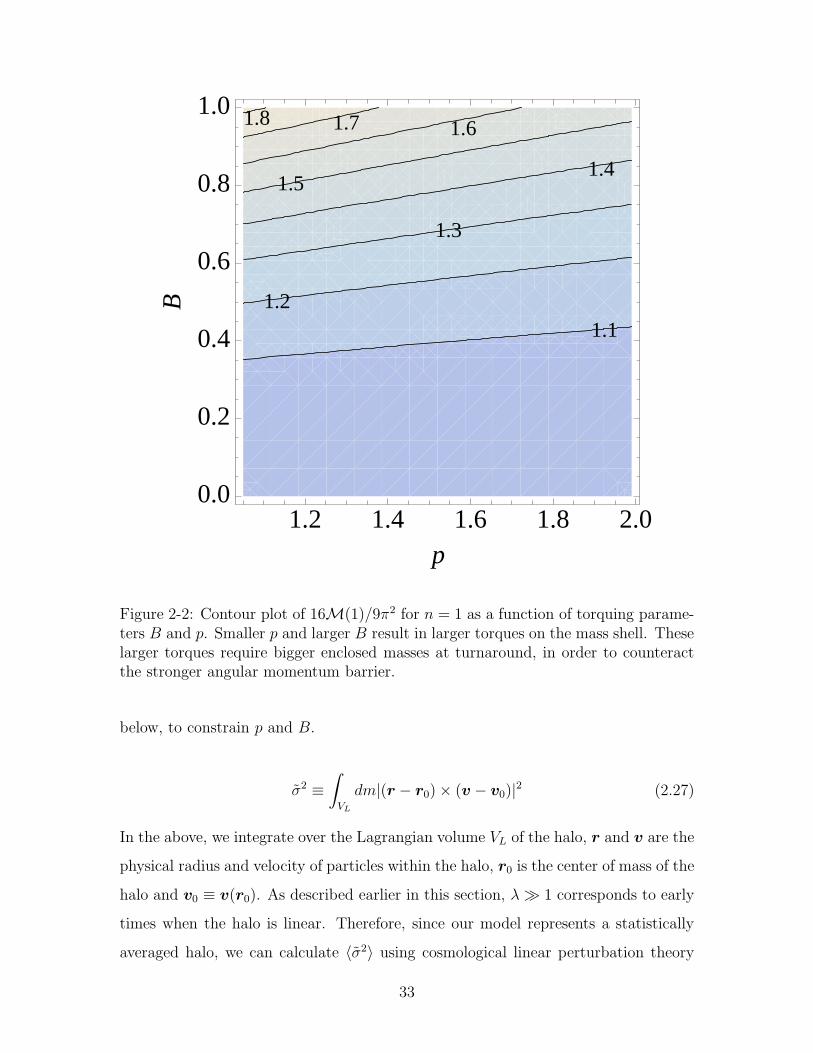
evolve λ and M and choose λ0, δ1 such that turnaround occurs (dλ/dξ = −λβ)when λ = 1. The free parameters for evolution before turnaround are n,B, p. Forthe zero angular momentum case analyzed in FG, the enclosed mass is the same
regardless of n; M(1) = (3π/4)2. Including torque, however, we find that the en-
closed mass depends on the parameters B and p. Figure 2-2 shows a contour plot of
16M(1)/9π2 for n = 1. As expected, the enclosed mass at turnaround must be larger
than the no-torque case in order to overcome the additional angular momentum bar-
rier. B sets the amplitude of the angular momentum while p controls how the angular
momentum grows in comparison to the mass perturbation. Larger B and smaller p
correspond to stronger torques on the mass shell. Contour plots with different values
of n give the same features.
The above perturbative scheme ensures that the inclusion of angular momentum
preserves cosmological initial conditions. Analyzing eq. (2.19) for ξ → −∞, and using
eqs. (2.23) and (2.25), we see that since p > n, the angular momentum correction
is subdominant to the density perturbation correction. More importantly, at early
times, the shell moves with the Hubble flow. Last, in order to be consistent with
cosmological initial conditions, the angular momentum of particles within a mass
shell must vanish at early times. Imposing r ∝ t2/3, and plugging into eq. (2.8), we
find that L ∝ t(1+p/n)/3. Hence, for all values of p we consider, the angular momentum
vanishes at early times and has a value of Br2∗/t∗ at turnaround. Note that shells
which turn around later have larger angular momentum.
2.3.1 Tidal Torque Theory
According to Hoyle’s tidal torque mechanism, mass shells before turnaround gain
angular momentum through their interactions with the tidal fields of neighboring
protogalaxies (Hoyle, 1951). Peebles (1969) claimed that the angular momentum
of protogalaxies in an Einstein de-Sitter universe grows as t5/3 while Doroshkevich
(1970) showed that for non-spherical regions, the angular momentum grows as t.
White (1984) confirmed Doroshkevich’s analysis with N-body simulations. Since the
net angular momentum of our model’s halo vanishes, we will instead use σ2, defined
32
1.11.2
1.3
1.41.5
1.61.71.8
1.2 1.4 1.6 1.8 2.00.0
0.2
0.4
0.6
0.8
1.0
p
B
Figure 2-2: Contour plot of 16M(1)/9π2 for n = 1 as a function of torquing parame-ters B and p. Smaller p and larger B result in larger torques on the mass shell. Theselarger torques require bigger enclosed masses at turnaround, in order to counteractthe stronger angular momentum barrier.
below, to constrain p and B.
σ2 ≡∫
VL
dm|(r − r0)× (v − v0)|2 (2.27)
In the above, we integrate over the Lagrangian volume VL of the halo, r and v are the
physical radius and velocity of particles within the halo, r0 is the center of mass of the
halo and v0 ≡ v(r0). As described earlier in this section, λ≫ 1 corresponds to early
times when the halo is linear. Therefore, since our model represents a statistically
averaged halo, we can calculate 〈σ2〉 using cosmological linear perturbation theory
33
and compare to expectations from our model.
Using the Zel’dovich approximation (Zel’dovich, 1970), assuming a spherical La-
grangian volume with radius R, and working to first order, we find:
⟨
σ2⟩
M= 6a4D2Mx2maxA
2(R) (2.28)
where M is the mass of the halo, a is the scale factor, D is the linear growth factor,
dots denote derivatives with respect to proper time, xmax is the lagrangian radius of
the volume, R is the spherical top hat radius for a halo of massM and A(R) is a time
independent function defined in Appendix A.2 which has units of length. Note that
the scale factor a and D are the only quantities which vary with time. For a matter
dominated universe, (〈σ2〉M)1/2 ∝ t, just as in the White analysis. This is expected
since the Lagrangian mass is time independent.
Next we calculate eq. (2.27) from the perspective of our model. Using eqns. (2.8),
(2.10), and (2.12) and assuming first order corrections to M are negligible, we find:
σ2 =
∫ rmax
rmin
B2 r4ta
t2λ−2γ ∂M(r, t)
∂rdr =
4π
3− 2γ
B2ρB(t)r7ta(t)
t2[
λ3−2γmax (t)− λ3−2γ
min (t)]
(2.29)
The lower limit of integration sets an effective smoothing length which we choose to
be λ ≫ 1 so that we only count shells that are still described by linear theory. The
upper limit of integration is required since all the mass in the universe does not go
into the halo. Since p = 2γ + 4 and n < p < 2n, then for the range of n we consider,
2γ < 3 and the angular momentum of the protogalaxy is dominated by shells close
to rmax. Equating eqs. (2.28) and (2.29) and assuming the first order corrections to
rmax in eq. (2.19) are negligible, we find p = 2n and:
B =2
3
√
2(7− 2n)M(1)(n−1)/3A(R)
R(2.30)
Eqs. (2.28) and (2.30) are derived in Appendix A.2. Note that the perturbative
34
analysis, presented above, which is used to calculate M(1) is not valid for p = 2n.
Redoing the analysis for this special case, we find:
α2 =4
3(2.31)
δ2 =9
14B2(2n− 3) +
(7n− 17)(2n− 3)
7(n− 3)2δ21 (2.32)
λ2 =9
14λ−2n0
(
B2 − 2
3
δ21(n− 3)2
)
(2.33)
For the remainder of this chapter we impose p = 2n, so that angular momentum
grows in accordance with cosmological perturbation theory, and set n according to
the halo mass. Unfortunately, when comparing to N-body simulations (Section 2.6.1),
eq. (2.30) overestimates the angular momentum of particles at turnaround by a factor
of 1.5 to 2.3. We discuss possible reasons for this discrepancy in Appendix A.2. For
convenience, B1.5 (B2.3) denotes B calculated using eq. (2.30) with the right hand
side divided by 1.5 (2.3). As described above, M(1) in eq. (2.30) depends on B.
Therefore, in order to find B, we calculate B and M(1) iteratively until eq. (2.30) is
satisfied.
The relationship between n and neff as well as tidal torque theory implies that
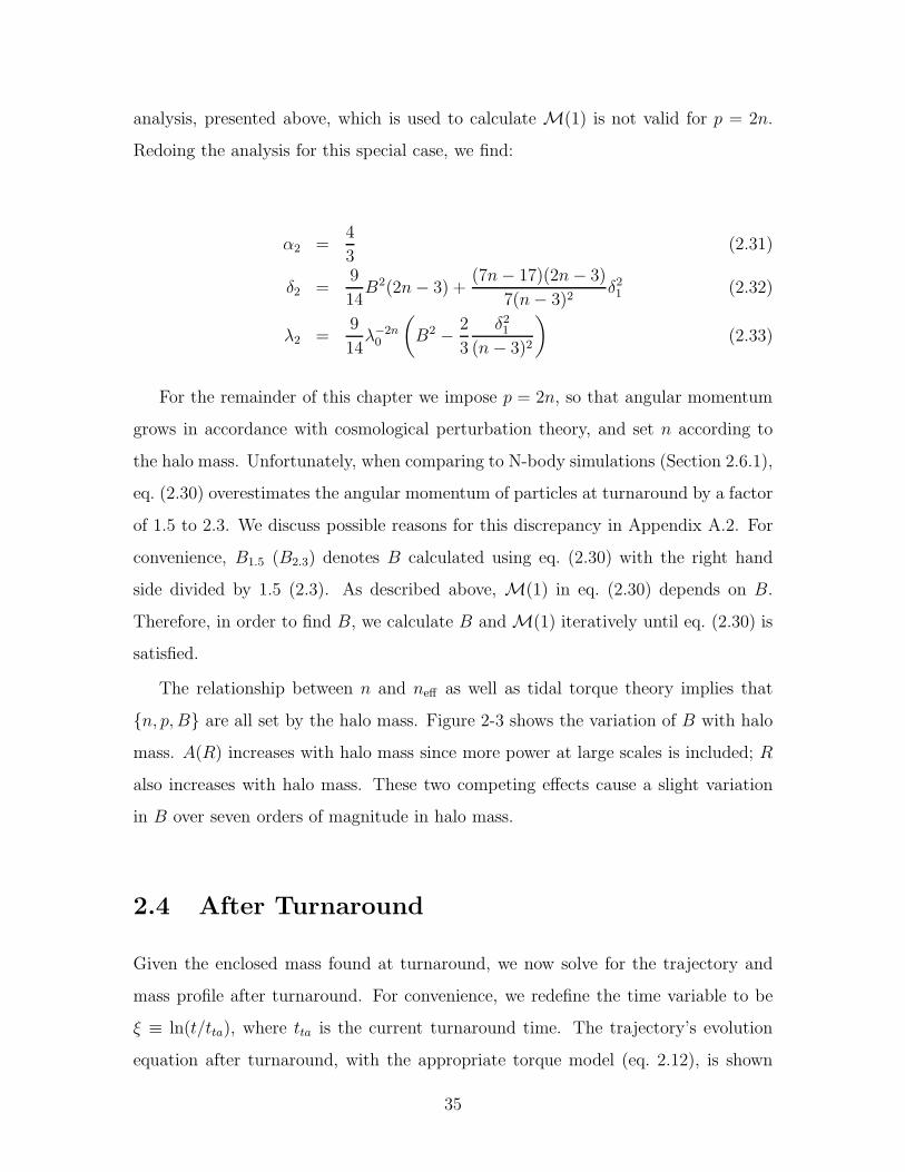
n, p, B are all set by the halo mass. Figure 2-3 shows the variation of B with halo
mass. A(R) increases with halo mass since more power at large scales is included; R
also increases with halo mass. These two competing effects cause a slight variation
in B over seven orders of magnitude in halo mass.
2.4 After Turnaround
Given the enclosed mass found at turnaround, we now solve for the trajectory and
mass profile after turnaround. For convenience, we redefine the time variable to be
ξ ≡ ln(t/tta), where tta is the current turnaround time. The trajectory’s evolution
equation after turnaround, with the appropriate torque model (eq. 2.12), is shown
35
8 9 10 11 12 13 14 150.3
0.4
0.5
0.6
0.7
0.8
0.9
1.0
log10HMML
B
Figure 2-3: The variation of model parameter B with halo mass. B sets the angularmomentum of particles at turnaround.
below.
d2λ
dξ2+ (2β − 1)
dλ
dξ+ β(β − 1)λ = −2
9
M(λ)
λ2+B2
λ3e2(+1−2β)ξ (2.34)
The torque model after turnaround was chosen to not explicitly depend on r, since
r begins to oscillate on a much faster timescale than the growth of the halo. Nusser
(2001) and Sikivie et al. (1997) focused on the case = 0. However, as was discussed
before, this results in density profiles steeper than what is predicted by numerical
simulations.
There are a number of dynamical processes that can cause a particle’s angular
momentum to evolve after turnaround. Dynamical friction (Chandrasekhar, 1943)
transfers the angular momentum of massive bound objects – like black holes, globular
clusters and merging satellite galaxies – to the background halo. A massive black
hole at the center of the halo that dominates the potential at small scales tends to
make the velocity dispersion isotropic (Gerhard & Binney, 1985; Merritt & Quinlan,
1998; Cruz et al., 2007). Bars (Kalnajs, 1991; Dehnen, 2000) and supermassive black
36
hole binaries (Milosavljevic & Merritt, 2003; Sesana et al., 2007) are also expected
to perturb the dark matter velocity distribution. While the torque model proposed
after turnaround is clearly very simplistic and may not accurately describe some of
the above phenomena, it still allows us to get intuition for how torques acting on
mass shells change the structure of the halo.
Analytically calculating is difficult since the halo after turnaround is nonlinear.
In Appendix A.3, we show in a simplistic manner how is sourced by substructure
and argue that dark matter dominated substructure should cause steeper density
profiles than baryon dominated substructure. In order to properly constrain , N-
body simulations are required. This is beyond the scope of this work.
The initial conditions for eq. (2.34), enforced in the above section, are λ(ξ = 0) = 1
and dλ/dξ(ξ = 0) = −β. As discussed before, self-similarity implies that all mass
shells follow the same trajectory λ(ξ). Hence, λ(ξ) can either be interpreted as
labeling the location of a particular mass shell at different times, or labeling the
location of all mass shells at a particular time. We take advantage of the second
interpretation in order to calculate the mass profile.
After turnaround, shells cross since dark matter is collisionless. Therefore, the
mass interior to a particular shell does not stay constant. However, since λ(ξ) specifies
the location of all mass shells at a particular time, the mass interior to a given scale
is simply the sum of all mass shells interior to it. The mass profile is then given by
(Bertschinger, 1985; Fillmore & Goldreich, 1984):
M(λ) =2
nM(1)
∫ ∞
0
dξ exp[−(2/n)ξ]H [λ− λ(ξ)]
= M(1)∑
i
(−1)i−1 exp[−(2/n)ξi] (2.35)
where M(1) is the normalization constant found in the prior section, H [u] is the
Heaviside function, and ξi is the ith root that satisfies λ(ξ) = λ. The above is
straightforward to interpret. The roots ξi label shell crossings at a particular scale
and the exponential factor accounts for the mass difference between shells that turn
37
around at different times.
Since the trajectory and the mass profile depend on each other, it is necessary to
first assume a mass profile, then calculate the trajectory from eq. (2.34) and resulting
mass profile from eq. (2.35) and repeat until convergence is reached.
The density profile D(λ) is straightforward to derive using eqs. 2.9, 2.10 and 2.35.
We find (Bertschinger, 1985; Fillmore & Goldreich, 1984):
D(λ) =1
3λ2dMdλ
=2
3n
M(1)
λ2
∑
i
(−1)i exp[−(2/n)ξi]
(
dλ
dξ
)−1
i
(2.36)
2.5 Asymptotic Behavior
Unlike N-body experiments, self-similar systems are not limited by resolution. One
can analytically infer the asymptotic slope of the mass profile close to the origin.
FG did this by taking advantage of adiabatic invariance, self-consistently calculating
the mass profile, and analyzing the limit of the mass profile as λ → 0. Below, we
generalize their analysis to the case of particles with changing angular momentum.
Unlike Nusser (Nusser, 2001), we do not restrict our analysis to the case = 0.
Just as in FG, we start by parameterizing the halo mass and the variation of the
apocenter distance ra.
M(r, t) = κ(t)rα (2.37)
rar∗
=
(
t
t∗
)q
(2.38)
In the above r∗ is the turnaround radius of a mass shell which turns around at t∗. It
is possible to relate q and α to n by taking advantage of adiabatic invariance. The
equation of motion for the mass shell is:
d2r
dt2= −Gκ(t)rα−2 +
L2(t)
r3(2.39)
At late times, the orbital period is much smaller than the time scale for the mass
38
and angular momentum to grow. Taking κ(t) and L(t) to stay roughly constant over
an orbit and integrating the above equation, we find the energy equation:
(
dr
dt
)2
=2Gκ(t)
α− 1(rα−1
a − rα−1)− L2(t)(r−2 − r−2a ) (2.40)
The above relationship tells us how the pericenters rp evolve with time. Note that
we only consider torquing models (eq. 2.12) which give rise to bound orbits. This
restriction on will be discussed below. Defining y ≡ rp/ra and evaluating the above
at r = rp, we find:
1− yα−1
y−2 − 1≡ A(y) =
(α− 1)L2(t)
2Gκ(t)rα+1a (t)
(2.41)
For > (<) 0, the angular momentum of particles in the mass shell increases (de-
creases). This gives rise to pericenters that increase (decrease). Hence at late times,
the orbit of a mass shell with increasing angular momentum will circularize and have
y ∼ 1, while the orbit of a mass shell with decreasing angular momentum will become
more radial, with y ≪ 1. With this in mind, we can now calculate the radial action
in order to find how q relates to n and α. The radial action is given by:
J = 2
∫ ra
rp
dr
(
dr
dt
)
= 2
(
2Gκ(t)
α− 1
)1/2
r(α+1)/2a
∫ 1
y(t)
du[
(1− uα−1)−A(y)(u−2 − 1)]1/2
(2.42)
In the above we’ve assumed α > 1. Generalizing to the case α < 1 is straight-
forward. The special case α = 1 will be addressed later. For y(t) ≪ 1, the above
integral is dominated by the region in which y(t) ≪ u ≪ 1. Over this region, the
integrand is time independent and hence the same for all orbits. Therefore adiabatic
invariance implies κ(t)rα+1a = const. For y(t) ∼ 1, the orbit is circular, which implies
the radial action vanishes and L2(t) = Gκ(t)rα+1a . Using eq. (2.38), and noting that
κ(t) ∝ ts where s = 3β − 2− αβ, we find at late times:
39
q =
1α+1
2 + 23n[α(1 + n)− 3] if ≥ 0
23n(α+1)
[α(1 + n)− 3] if < 0
(2.43)
For the specific case, < 0, taking advantage of y ≪ 1, the adiabatic invariance
arguments above, and eqs. (2.8) and (2.12), we can rewrite eqn. (2.41) in the form
y(t, t∗) = y0(t/t∗)l, where:
l =
if α > 1,
2/(α+ 1) if α < 1.
(2.44)
and y0r∗ is the pericenter of a mass shell at turnaround. Constant angular momentum
after turnaround corresponds to = 0. This case was addressed analytically in
(Nusser, 2001) and numerically in (Sikivie et al., 1997).
We next take advantage of the functional form of the mass profile. Following FG,
we define P (r/ra, y) to be the fraction of time a particle with apocenter distance ra
and pericenter yra, at a particular time t, spends inside r.
P (v, y) = 0 (v < y)
P (v, y) =I(v, y)
I(1, y)(y < v ≤ 1)
P (v, y) = 1 (v > 1) (2.45)
where
I(v, y) ≡
∫ v
ydu
((1−uα−1)−A(y)(u−2−1))1/2if α > 1,
∫ v
ydu
((uα−1−1)+A(y)(u−2−1))1/2if α < 1.
(2.46)
We see that the presence of pericenters causes the new case v < y, which did not
exist in the FG analysis. Self consistency demands that
(
r
rta
)α
=M(r, t)
M(rta, t)=
∫ Mta
0
dM∗
Mta
P
(
r
ra(t, t∗), y(t, t∗)
)
(2.47)
40
whereM∗ is the mass internal to a shell that turns around at t∗ andMta is the current
turnaround mass. The integral assigns a weight to each shell depending on how often
that shell is below the scale r. Noting from eq. (2.10) that
M∗ =Mta
(
t∗t
)3β−2
, (2.48)
using eq. (2.38) and transforming integration variables, we find:
(
r
rta
)α−k
= k
∫ ∞
r/rta
du
u1+kP (u, y(t, t∗)) (2.49)
where
k =6
2 + n(2− 3q)(2.50)
As u increases, the above integral sums over shells with smaller t∗. Since the pericenter
of a shell evolves with time, the second argument of P depends on u. The dependence,
as we showed, varies with torque model (sign of ); hence we’ve kept the dependence
on u implicit. Next we analyze the above for certain regimes of r/rta, and certain
torquing models, in order to constrain the relationship between α and k.
2.5.1 Inner Solution; Negative Torque
For < 0, particles lose angular momentum over time. When probing scales r/rta ≪y0, mass shells with t∗ ≪ tta only contribute. As a result, y(t, t∗) ≪ 1. Using eq.
(2.44), we then find:
y(t, t∗) = y0
(
t
t∗
)l
= y0
(
r
urta
)δ
(2.51)
where δ ≡ l/(q − β). For bound mass shells, q − β < 0. Therefore, since δ > 0, the
first argument of P in eq. (2.49) increases while the second decreases as we sum over
shells that have turned around at earlier and earlier times (u→ ∞). For r/rta ≪ y0,
mass shells which most recently turned around do not contribute to the mass inside
r/rta since we are probing scales below their pericenters. Mass shells only begin to
41
contribute when the two argument of P are roughly equal to each other. This occurs
around:
u = y1 ≡(
y0(r/rta)δ)1/(1+δ)
(2.52)
Hence, we can replace the lower limit of integration in eq. (2.49) with y1. We next
want to calculate the behavior of eq. (2.49) close to y1 in order to determine whether
the integrand is dominated by mass shells around y1 or mass shells that have turned
around at much earlier times. The first step is to calculate the behavior of P (u, y)
for u ≈ y. We find:
P (u, y) ∝ u1/2(1− y/u)1/2 ×
y1/2 if α > 1,
y1−α/2 if α < 1.
(2.53)
Given the above, we evaluate the indefinite integral in eq. (2.49), noting that y is a
function of u (eq. 2.51). For u ∼ y1, we find:
∫
du
u1+kP
(
u, y0
(
r
urta
)δ)
∝ (u/y1 − 1)3/2
y1−k1 if α > 1,
y3/2−k−α/21 if α < 1.
(2.54)
Now comes the heart of the argument. Following the logic in FG, if we keep u/y1
fixed and the integrand blows up as r/rta → 0, then the left hand side of eq. (2.49)
must diverge in the same way as the right hand side shown in eq. (2.54). Therefore,
using eq. (2.52):
α− k =
δ(1− k)/(1 + δ) if α > 1,
δ(3/2− k − α/2)(1 + δ) if α < 1.
(2.55)
Otherwise, if the right hand side converges, then the integrand will not depend on
r/rta as r/rta → 0. Therefore, the left hand side cannot depend on r/rta either,
which implies α = k. Solving the above system of equations for α given eqs. (2.43)
42
and (2.50) and making sure the solution is consistent, (ie: using eq. (2.55) only if the
integrand diverges), we find:
For n ≤ 2 :
α =1 + n−
√
(1 + n)2 + 9n(n − 2)
3n
k =1 + n + 3n −
√
(1 + n)2 + 9n(n − 2)
n(4 + n)
q =1 + n− 3n −
√
(1 + n)2 + 9n(n − 2)
3n
For n ≥ 2 :
α = k =3
1 + n, q = 0 (2.56)
The above solutions are continuous at n = 2. Moreover, taking the no-torque limit
( → 0) for n ≤ 2 gives the same solutions as n ≥ 2, which is consistent with
analytic and numeric results from (Nusser, 2001; Sikivie et al., 1997). Taking the
limit, → −∞ reproduces the FG solution, as expected, since the shell loses its
angular momentum instantly. The solution for n ≥ 2 is independent of . This is
because the mass is dominated by shells with turnaround time t∗ ≪ tta which have
effectively no angular momentum. In other words, for < 0, the solution should
only depend on torquing parameters when the mass is dominated by shells that have
turned around recently.
2.5.2 Inner Solution; Positive Torque
For > 0, the angular momentum of particles increase with time. As mentioned
above, when probing scales r/rta ≪ y0, mass shells with t∗ ≪ tta only contribute.
As a result, y(t, t∗) ∼ 1. In other words, the orbits are roughly circular. We can
therefore replace the lower limit of integration in eq. (2.49) with 1 since mass shells
will only start contributing to the sum when u ∼ y ∼ 1. Hence, the right hand side
of eq. (2.49) does not depend on r/rta, which implies α = k. Using eq. (2.43) and
43
(2.50), we find:
α = k =3
1 + n− 3n, q = 2 , for 0 ≤ n ≤ 3 (2.57)
The no torque case, = 0, is consistent with the analysis in the prior subsection.
The singularity = (1 + n)/3n implies q = β. This physically corresponds to the
orbital radius of mass shells increasing at the same rate as the turnaround radius and
results in orbits that are not bound and a cored profile where there are no particles
internal to a particular radius. This breaks the assumption of a power law mass
profile (eq. 2.37); hence we only consider < (1 + n)/3n.
Unlike the Nusser solution, certain parameters give α > 3, which corresponds to
a density profile which converges as r → 0. Since the angular momentum acts like a
heat source dρ/dr > 0 is dynamically stable and physical.
2.5.3 Outer Solution
In this regime, we are probing scales larger than the pericenters of the most recently
turned around mass shells. As a result, P (u, y) is dominated by the contribution from
the integrand when u≫ y. Therefore:
P (u, y) ∝
u if α > 1,
u(3−α)/2 if α < 1.
(2.58)
Hence the integral in eq. (2.49) becomes:
∫
du
u1+kP (u, y(t, t∗)) ∝
u1−k if α > 1,
u3/2−k−α/2 if α < 1.
(2.59)
Following the logic in the prior section, if the integral diverges as r/rta → 0, then
we set the exponents on the left hand side and right hand side equal to each other
so that both sides diverge in the same way. If the integral converges, then the left
44
hand side cannot depend on r/rta, which implies α = k. Given these arguments, and
imposing consistency with the above inequalities on α to find the appropriate ranges
for n, we find:
α = 1 , k =6
4 + n, q =
n− 2
3n, for n ≤ 2
α = k =3
1 + n, q = 0 , for n ≥ 2 (2.60)
The above is exactly the FG solution. We expect to recover these solutions since
we are probing scales larger than the pericenters of the most massive shells, where
the angular momentum does not affect the dynamics.
This section assumed α 6= 1 and yet, for certain parts of parameters space, eqs.
(2.56), (2.57) and (2.60) give α = 1. However, since the solutions are continuous as
α→ 1 from the left and right, then the results hold for α = 1 as well.
2.6 Structure of the Halo
In this section, we discuss the radial structure of galactic size halos and compare
directly to numerical N-body simulations. Note however, that the mass of a halo is
not well defined when our model is applied to cosmological structure formation since
it is unclear how the spherical top hat mass which characterizes the halo when it is
linear relates to the virial mass which characterizes the halo when it is nonlinear. For
halos today with galactic size virial masses, we assume the model parameter n which
characterizes the initial density field, is set by a spherical top hat mass of 1012M⊙. As
described in prior sections, specifying the top hat mass also sets model parameters
B and p. Before comparing directly to N-body simulations, we first describe how
influences the halo.
Figure 2-4 shows the mass M(λ) and density profiles D(λ) for galactic size halos
n = 0.77, p = 2n,B1.5 = 0.39 with varying . The spikes in the density profile are
caustics which form at the shell’s turning points. They form because of unphysical
45
initial conditions; we assume each shell has zero radial velocity dispersion. The
structure of the halos naturally break down into three different regions. The dividing
points between these regions are roughly the virial radius (rv) and y0rta, the pericenter
of the mass shell which most recently turned around.
As in dark matter N-body simulations, we associate the virial radius with r200,
the radius at which M(r200) = 800πρBr3200/3 is satisfied. Numerically, we find that
the virial radius occurs near the first caustic (λ ∼ .18). For r > rv, the mass profile
flattens and then starts to increase. The flattening is equivalent to what is seen on
large scales in N-body simulations where ρ ∝ r−3. The mass profile then starts to
increase again because at large radii, where λ ≫ 1, the density is roughly constant,
which implies M ∝ λ3. For r ∼ rv, it is difficult to make analytic predictions for
the mass profile because adiabatic invariance breaks down. In other words, the mass
of the halo and angular momentum of a shell change on the same time scale as the
shell’s orbital period.
As discussed in the prior section, for y0rta ≪ r ≪ rv, we can take advantage
of adiabatic invariance to infer the logarithmic slope of the mass profile. Since this
regime probes a scale much larger than the pericenters of the mass shells, the angular
momentum does not affect the dynamics and we recover the FG solution. For our
particular choice of n = 0.77, this gives an isothermal profile with ρ ∝ r−2. However,
since n < 2 for all collapsed objects today (Figure 2-1) and based on the results of
FG, our model predict that all halos are isothermal in this regime.
Last, for r/rta ≪ y0, angular momentum begins to play a role and the halo starts
to exhibit different features than the FG solution. The behavior is very intuitive. The
mass of a particular shell does not contribute to the internal mass when probing radii
less than the pericenter of that mass shell. Therefore, as one probes radii smaller than
the pericenter of the most recently turned around mass shell, one expects a steeper fall
off than the FG solution, since less mass is enclosed interior to that radius. Moreover,
varying varies the pericenter of mass shells over time. Increasing (decreasing)
angular momentum, > (<) 0, causes the pericenters to increase (decrease) over
time. This results in profiles which are steeper (shallower) than the no-torque case.
46
0.001 0.01 0.1 1
1x10⁻⁶
1x10⁻⁵
1x10⁻⁴
0.001
0.01
0.1
1
ϖ = − 0.4ϖ = − 0.2ϖ = 0ϖ = 0.2ϖ = 0.4
λ
M(λ
)
rv∕rtay0
0.001 0.01 0.1 1
λ
10
100
1x10³
1x10⁴
1x10⁵
1x10⁶
D(λ
)
ϖ = − 0.4ϖ = − 0.2ϖ = 0ϖ = 0.2ϖ = 0.4
y0 rv∕rta
Figure 2-4: The mass and density profiles for galactic size halos n = 0.77, p =2n,B1.5 = 0.39 with varying . The value of changes how pericenters evolvewith time and thereby affects how many shells at a particular scale contribute to theinternal mass. The above numerically computed profiles match analytic predictions.The virial radius (rv) and first pericenter passage (y0rta) are labeled for clarity.
47
2 4 6 8 10 12 14
0.05
0.10
0.20
0.50
1.00
tt*
rr *
2 4 6 8 10 12 14
0.10
1.00
0.50
0.20
0.30
0.15
0.70
tt*
rr *
2 4 6 8 10 12 14
1.00
0.50
0.20
0.30
0.15
0.70
tt*
rr *
Figure 2-5: The radius of a mass shell, normalized to its turnaround radius, for agalactic size halo n = 0.77, p = 2n,B1.5 = 0.39, plotted vs time. The top panelshows a shell with particles that have decreasing angular momentum ( = −0.2).The middle panel shown a shell with particles that have constant angular momentum( = 0). The bottom panel shows a shell with particles that have increasing angularmomentum ( = 0.2).
48
0.01 0.02 0.05 0.10 0.20 0.50 1.00
-4
-2
0
2
4
Λ
t * r *
dr dt
0.01 0.02 0.05 0.10 0.20 0.50 1.00
-4
-2
0
2
4
Λ
t * r *
dr dt
0.01 0.02 0.05 0.10 0.20 0.50 1.00
-4
-2
0
2
4
Λ
t * r *
dr dt
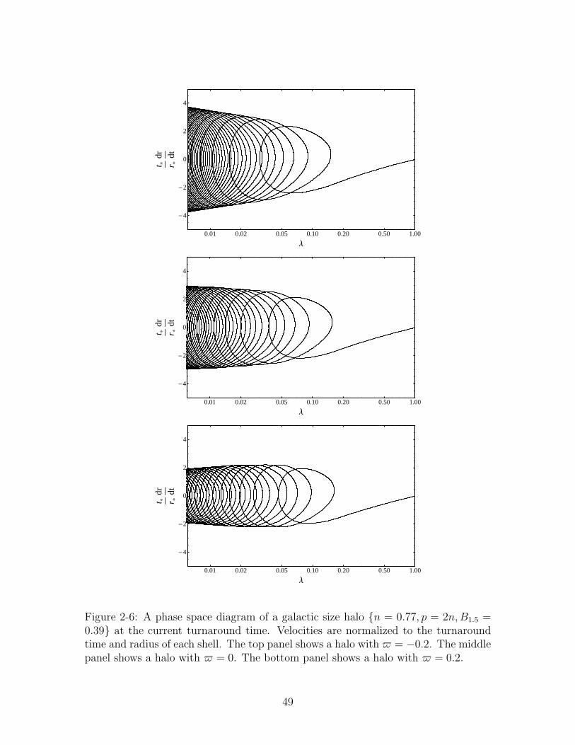
Figure 2-6: A phase space diagram of a galactic size halo n = 0.77, p = 2n,B1.5 =0.39 at the current turnaround time. Velocities are normalized to the turnaroundtime and radius of each shell. The top panel shows a halo with = −0.2. The middlepanel shows a halo with = 0. The bottom panel shows a halo with = 0.2.
49
It is informative to find how the transition radius y0 depends on model parameters.
Since the mass and angular momentum grow significantly before the first pericenter,
we can only approximately determine this relationship. We assume that the profile is
isothermal on large scales and the halo mass and shell angular momentum are fixed
to their turnaround values. For y0 ≪ 1, the transitional radius y0 solves the transcen-
dental equation y20 ln(y0) = −9B2/4M(1). As expected, B → 0 reproduces y0 → 0.
As shown in Figure 2-2, M(1) varies with B, p. However, for reasonable parameter
values, the mass normalization is changed at most by a factor of 2. Therefore, y0 most
strongly depends on B, and p has a negligible effect on the structure of the halo. As
seen in figure 2-4, y0 should also depends on . The above approximation neglects
this dependence since we assumed the angular momentum is set to the turnaround
value.
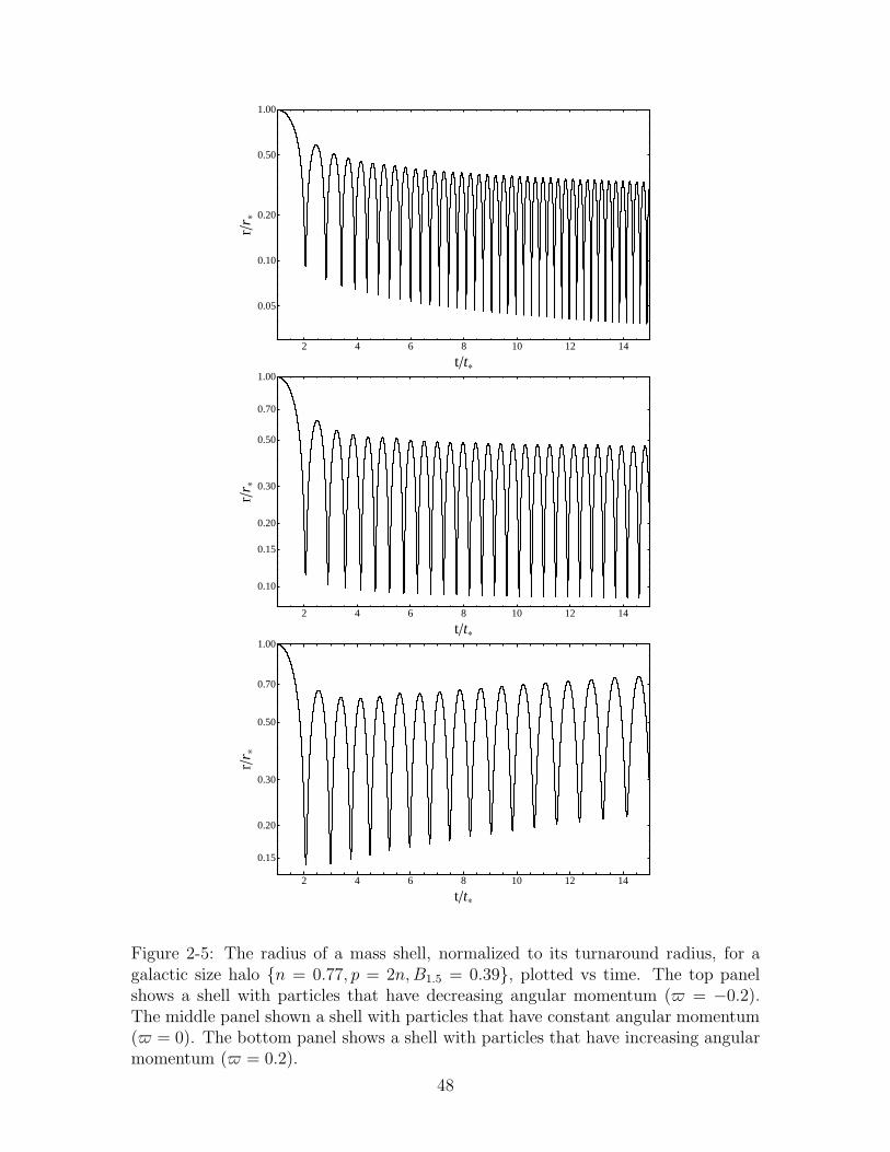
Figure 2-5 shows the radius of a mass shell, normalized to its turnaround radius
r∗, for a galactic size halo n = 0.77, p = 2n,B1.5 = 0.39, as a function of time. In
the top panel, particles in the shell lose angular momentum ( = −0.2), in the middle
panel the angular momentum remains constant ( = 0), while in the bottom panel
particles in the shell gains angular momentum ( = 0.2). As expected, the pericenters
in the top panel decrease with time while the pericenters grow in the bottom panel.
Hence, the orbits of particles with decreasing angular momentum become more radial
while those with increasing angular momentum become more circular.
Notice that the period of oscillation also varies for different . The period of
oscillation is set by the shell’s apocenter ra and the mass internal to ra. Using the
adiabatic invariance relations we found in Section 2.5 and assuming Kepler’s third
law, we find that the period of the orbit P ∝ r2a for shells with decreasing angular
momentum and P ∝ ra for shells with increasing angular momentum. Moreover,
from eqs. (2.56) and (2.60), ra decreases (increases) with time for < (>) 0. Though
Kepler’s third law doesn’t hold for this system, it still gives intuition for the above
results.
Figure 2-6 shows the phase space diagram for a galactic size halo n = 0.77, p =
2n,B1.5 = 0.39. In the top panel, the particles in the shell lose angular momentum
50
( = −0.2), in the middle panel the angular momentum remains constant ( = 0),
while in the bottom panel the particles in the shell gain angular momentum ( = 0.2).
The diagram labels the phase space point of every shell at the current turnaround
time. All radial velocities are normalized to the shell’s turnaround time t∗ and radius
r∗. Unlike FG, the presence of angular momentum results in caustics associated with
pericenters as well, which can be seen in the lower panel of Figure 2-4. In addition,
since an increasing angular momentum results in increasing pericenters, the pericenter
caustics are more closely spaced in the lower panel than in the upper panel. Moreover,
the amplitude of the radial velocity is smaller in the lower panel because orbits are
circularizing. The phase space curve appears to intersect itself because we did not
plot the tangential velocity component. In full generality, the distribution in the
phase space (r, vr, vt = L/r) for our model is a non-self-intersecting one-dimensional
curve.
2.6.1 Comparing with N-body Simulations
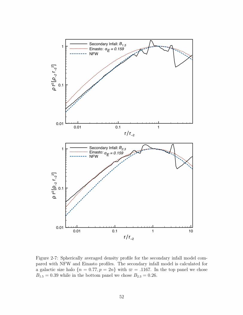
In this subsection, we compare the density profile of our model’s halo to empirical
fits inspired by N-body simulations. We first numerically calculate the density profile
for a galactic size halo with = 0.12. This value of was chosen so that ρ ∝ r−1
on small scales. We then compute the spherically averaged density in 50 spherical
shells equally spaced in log10 r over the range 1.5 × 10⁻⁴ < r/rv < 3, and take
rv = r200 (defined above). This is the same procedure followed with the recent
Aquarius simulation (Navarro et al., 2010). Next, we calculate r−2, the radius where
r2ρ reaches a maximum. For our halo, as discussed above, the profile is isothermal
over a range of r. Moreover, the maximum peaks associated with the caustics are
unphysical. So, we choose a value of r−2 in the isothermal regime that gives good
agreement with the empirical fits. Changing r−2 does not change our interpretation
of the results.
In Figure 2-7 we compare our spherically averaged density profile to NFW and
Einasto profiles. We plot r2ρ in order to highlight differences. The NFW profile is
given by (Navarro et al., 1996):
51
0.01 0.1 10.01
0.1
1Secondary Infall:
Einasto:
NFW
r∕r−2
ρ r
2 [ρ
−2 r
−2
2]
αE = 0.159
B1.5
0.01 0.1 1 100.01
0.1
1 Secondary Infall:Einasto:NFW
r∕r−2
ρ r
2 [ρ
−2 r
−2
2]
αE
= 0.159
B2.3
Figure 2-7: Spherically averaged density profile for the secondary infall model com-pared with NFW and Einasto profiles. The secondary infall model is calculated fora galactic size halo n = 0.77, p = 2n with = .1167. In the top panel we choseB1.5 = 0.39 while in the bottom panel we chose B2.3 = 0.26.
52
ρ(r) =4ρ−2
(r/r−2)(1 + r/r−2)2(2.61)
while the Einasto profile is given by:
ln[
ρ(r)/ρ−2
]
= (−2/αE)[(r/r−2)αE − 1] (2.62)
where ρ−2 is the density of our halo at r−2 and αE , known as the shape parameter,
sets the width of the r2ρ peak. In the top panel, we use B1.5 = .39 while in the
bottom panel, we use B2.3 = .26. We choose αE = 0.159 since this value was used in
Figure 3 of Navarro et al. (2010).
We see that the secondary infall model works surprisingly well. The peaks are
a result of the caustics that arise because of cold radial initial conditions. The first
spike on the right comes from the first apocenter passage while the second comes from
the first pericenter passage. The location of pericenter is most strongly influenced
by the model parameter B. Hence, the isothermal region is smaller in the top panel
than in the bottom panel since particles have less angular momentum at turnaround
in the lower panel than in the upper panel. The parameter B then plays the same role
as αE ; it sets the width of the isothermal region. If we assume N-body simulations
faithfully represent dark matter halos, then Figure 2-7 implies that our estimate of B
in eq. (2.30) overestimates the actual value by 1.5 to 2.3. We discuss possible reasons
for this in Appendix A.2.
2.7 Discussion
N-body simulations reveal a wealth of information about dark matter halos. Older
simulations predict density profiles that are well approximated by an NFW profile
(Navarro et al., 1996), while more recent simulations find density profiles that fit bet-
ter with a modified NFW profile (Moore et al., 1999) or the Einasto profile (Navarro
et al., 2010). In an attempt to gain intuition for these empirical profiles, we’ve gen-
eralized the self-similar secondary infall model to include torque. This model doesn’t
53
suffer from resolution limits and is much less computationally expensive than a full
N-body simulation. Moreover, it is analytically tractable. Using this model, we were
able to analytically calculate the density profile for r/rta ≪ y0 and y0 ≪ r/rta ≪ 1.
Note that the self-similar framework we’ve extended predicts power law mass profiles
on small scales. Hence, it is inconsistent with an Einasto profile.
It is clear from our analysis that angular momentum plays an essential role in
determining the structure of the halo in two important ways. First, the amount
of angular momentum at turnaround (B) sets the width of the isothermal region.
Second, the presence of pericenters softens the inner density slope relative to the
FG solution because less mass shells contribute to the enclosed mass. Moreover, the
interior density profile is sensitive to the way in which particles are torqued after
turnaround ().
If we assume that is constant for all halos, then this secondary infall model
predicts steeper interior density profiles for larger mass halos. More specifically, if we
use the value of = 0.12 which gave ρ ∝ r−1 for galactic size halos, then ρ ∝ r−0.66 for
a 108M⊙ halo and ρ ∝ r−1.42 for a 1015M⊙ halo. This trend towards steeper interior
slopes for larger mass halos, and hence non-universality, has been noticed in recent
numerical simulations (Ricotti et al., 2007; Cen et al., 2004) as well as more general
secondary infall models (Del Popolo, 2010). On the other hand, if we assume that all
halos have ρ ∝ r−1 as r → 0, then must vary with halo mass. More specifically,
halos with mass M < 109M⊙ must have particles which lose angular momentum
over time ( < 0) while halos with mass M > 109M⊙ must have particles which
gain angular momentum over time ( > 0). In other words, in order for our self-
similar framework to predict universal density profiles, must conspire to erase any
dependence on initial conditions. A more thorough treatment requires the use of
N-body simulations, which is beyond the scope of this chapter.
It is also possible to predict a dark matter halo’s density distribution if one assumes
a mapping between a mass shell’s initial radius, when the structure is linear, to its final
average radius, which is some fraction of its turnaround radius. From this scheme,
one can also infer a velocity dispersion, using the virial theorem. Unfortunately, this
54
scheme does not give any information about the halo’s velocity anisotropy. Our self-
similar prescription discussed above, on the other hand, contains all of the velocity
information. Hence, one can reconstruct the velocity anisotropy profile given the
trajectory of a mass shell. The velocity anisotropy is significant since it describes to
what degree orbits are radial. Moreover, it can break degeneracies between n and
in our halo model. We will discuss the velocity structure of our halo model, including
the pseudo-phase-space density profile, in more detail in Paper 2 of this series. There
we will once again compare our halo predictions to the recent Aquarius simulation
results (Navarro et al., 2010).
While the above self-similar prescription has its clear advantages, it’s also un-
physical since mass shells at turnaround are radially cold. The same tidal torque
mechanisms which cause a tangential velocity dispersion (Hoyle, 1951), should also
give rise to a radial velocity dispersion. For a more physical model, one would need
to impose self-similarity to a phase space description of the halo and include sources
of torque as diffusion terms in the Boltzmann equation. This will be the subject of
Paper 3 of this series.
As we’ve shown, the way in which particles are torqued after turnaround () in-
fluences the interior power law of the density profile. One way to source this change in
angular momentum is through substructure that is aspherically distributed through-
out the halo. It is reasonable to assume that substructure dominated by baryons
torque halo particles more strongly than substructure dominated by dark matter since
baryons can achieve higher densities and hence are not tidally disrupted as easily. If
this is the case, then torques sourced by baryons would result in a larger value of
than torques sourced by dark matter. According to the predictions of this secondary
infall model, this would lead to less cuspy profiles (See Appendix A.3 for a more
detailed discussion). Therefore a more thorough understanding of coupled with
this simplified model of halo formation could potentially shed light on the Cusp Core
problem and thereby possibly bridge the gap between simulations and observations.
55
56
Chapter 3
Velocity Structure of Self-Similar
Spherically Collapsed Halos1
Abstract
Using a generalized self-similar secondary infall model, which accounts for tidaltorques acting on the halo, we analyze the velocity profiles of halos in order togain intuition for N-body simulation results. We analytically calculate the asymp-totic behavior of the internal radial and tangential kinetic energy profiles in differentradial regimes. We then numerically compute the velocity anisotropy and pseudo-phase-space density profiles and compare them to recent N-body simulations. Forcosmological initial conditions, we find both numerically and analytically that theanisotropy profile asymptotes at small radii to a constant set by model parameters.It rises on intermediate scales as the velocity dispersion becomes more radially domi-nated and then drops off at radii larger than the virial radius where the radial velocitydispersion vanishes in our model. The pseudo-phase-space density is universal on in-termediate and large scales. However, its asymptotic slope on small scales dependson the halo mass and on how mass shells are torqued after turnaround. The resultslargely confirm N-body simulations but show some differences that are likely due toour assumption of a one-dimensional phase space manifold.
3.1 Introduction
Recent N-body simulations have revealed a wealth of information about the velocity
structure of halos (Navarro et al., 2010; Ludlow et al., 2010; Vogelsberger et al.,
1This chapter is based on the published paper Zukin & Bertschinger 2010b
57
2010). However, simulations have finite dynamic range. Moreover, it is difficult
to draw understanding from their analysis, and computational resources limit the
smallest resolvable radius, since probing smaller scales require using more particles
and smaller time steps. Hence, it seems natural to use analytic techniques, which do
not suffer from resolution limits, to analyze the velocity distributions of halos.
Numerous authors have analytically investigated the density profiles of halos.
Work began with Gunn and Gott where they analyzed the continuous accretion of
mass shells onto an initial overdensity (Gunn & Gott, 1972; Gott, 1975; Gunn, 1977).
This process is known as secondary infall. By imposing that the mass accretion is self-
Conveniently both p and B are set by the halo mass. However, after comparing to
density profiles from N-body simulations, we found that our expression for B derived
from linear theory overestimates the actual value. Hence, for the rest of this chapter,
the notation B1.5 (B2.3) signifies using a value of B divided by 1.5 (2.3).
Model parameter , defined above, sets how quickly the angular momentum of
particles grows after turnaround. This parameter is difficult to constrain analytically
since the halo is nonlinear after turnaround. However, in Chapter I we showed that a
nonzero can be sourced by substructure. Moreover, influences the density profile
at small scales since it controls how the pericenters of shells evolve over time.
The trajectory of a shell after turnaround contains all of the velocity information
60
in the halo. The trajectory’s evolution equation, which follows from Newton’s law, is
given by:
d2λ
dξ2+ (2β − 1)
dλ
dξ+ β(β − 1)λ = −2
9
M(λ)
λ2+B2
λ3e2(+1−2β)ξ (3.5)
where ξ ≡ ln(t/tta) and tta is the current turnaround time. The initial conditions for
eq. (3.5) are λ(ξ = 0) = 1 and dλ/dξ(ξ = 0) = −β. Calculating M(1) requires evolv-
ing both the shell’s trajectory and M(λ) before turnaround (Zukin & Bertschinger,
2010a). Because of self-similarity, the trajectory λ(ξ) can either be interpreted as
labeling the location of a particular mass shell at different times, or labeling the
location of all mass shells at a particular time. We take advantage of the second
interpretation in order to numerically calculate the velocity profiles.
Inside the shell that is currently at its second apocenter, multiple shells exist at all
radii. This can be seen from Figure 5 of (Bertschinger, 1985), which plots the location
of all shells at a particular time. Therefore the expectation value of a quantity h, for
example the radial velocity, at radius r and time t is the value of h for each shell at
r weighted by each shell’s mass. We find:
〈h(r, t)〉 =∫Mta
0dM∗
Mtah(t, t∗)δ
D(
λ− λ(ξ))
∫Mta
0dM∗
MtaδD(
λ− λ(ξ))
(3.6)
where Mta is the current turnaround mass, h(t, t∗) represents the value of h for the
shell with turnaround time t∗, dM∗ is the mass of the shell with turnaround time t∗,
and δD is the dirac delta function which picks out all shells at r.
In order to numerically calculate h, we must relate h(t, t∗) to λ(ξ), the computed
trajectory of the shell which turns around at tta. Using self-similarity, we find:
vt(t, t∗) = Brtate(1+−2β)ξ∗
1
λ(ξ∗)(3.7)
vr(t, t∗) =rtate−βξ∗
d
dξ
[
eβξλ(ξ)]
|ξ=ξ∗ (3.8)
where ξ∗ ≡ t/t∗ and vt (vr) is the tangential (radial) velocity. Using eqs. (3.6)-(3.8),
61
and taking advantage of the delta function, the tangential (σ2t ) and radial (σ2
r ) velocity
dispersions become:
σ2t (r, t) ≡
⟨
v2t (r, t)⟩
=r2tat2
∑
i e(4−7β+2)ξiλ−2
i |dλ/dξ|−1i
∑
i e(2−3β)ξi |dλ/dξ|−1
i
(3.9)
σ2r(r, t) ≡
⟨
v2r(r, t)⟩
− 〈vr(r, t)〉2
=r2tat2
∑
i e(2−5β)ξi
[
d(eβξλ)/dξ]2
i|dλ/dξ|−1
i∑
i e(2−3β)ξi |dλ/dξ|−1
i
− r2tat2
(
∑
i e(2−4β)ξi
[
d(eβξλ)/dξ]
i|dλ/dξ|−1
i∑
i e(2−3β)ξi |dλ/dξ|−1
i
)2
(3.10)
where ξi is the ith root that satisfies λ = λ(ξ). In the above, we’ve imposed 〈vt(r, t)〉 =0 since our model assumes that the orbital planes of particles in a given shell are
oriented in random directions. Note that inside the shell that is currently at its
second apocenter, interference between multiple shells forces 〈vr(r, t)〉 to quickly go
to zero.
3.3 Asymptotic Behavior
Here, using techniques developed in (Fillmore & Goldreich, 1984), we analytically
calculate the logarithmic slope of the tangential and radial kinetic energy in two dif-
ferent radial regimes. We accomplish this by taking advantage of adiabatic invariance
and self consistently calculating the total radial and tangential kinetic energy profiles
of the halo.
We start by parametrizing the halo mass, radial kinetic energy Kr, tangential
kinetic energy Kt and the variation of the apocenter distance ra.
62
M(r, t) = κ(t)rα (3.11)
Kr(r, t) = κr(t)rαr (3.12)
Kt(r, t) = κt(t)rαt (3.13)
rar∗
=
(
t
t∗
)q
(3.14)
In the above r∗ is the turnaround radius of a mass shell that turns around at t∗. As
was shown in Chapter I, adiabatic invariance allows us to relate q and α to n. At
late times, the orbital period is much smaller than the time scale for the mass and
angular momentum to grow. Integrating Newton’s equation and assuming κ(t) and
L(t) change little over an orbit, we find:
(
dr
dt
)2
=2Gκ(t)
α− 1(rα−1
a − rα−1)− L2(t)(r−2 − r−2a ). (3.15)
The above relationship tell us how the pericenters rp evolve with time. Defining
y ≡ rp/ra and evaluating the above at r = rp, we find:
1− yα−1
y−2 − 1≡ A(y) =
(α− 1)L2(t)
2Gκ(t)rα+1a (t)
(3.16)
In Chapter I, by analyzing the radial action, we found that when y ≪ 1, κ(t)rα+1a (t) =
const. Therefore, for < 0, eq. (3.16) implies that y will decrease over time. How-
ever, for > 0, κ(t)rα+1a (t) = const and eq. (3.16) imply that y will increase over
time and will at one point violate y ≪ 1. Since we only consider bound orbits, the
constraint y ≤ 1 holds. At late times, as the angular momentum continues to increase
for > 0, y ∼ 1, orbits become approximately circular, the radial action vanishes,
and L2(t) ∼ κ(t)rα+1a (t). Hence halos with < 0 will have orbits that become more
radial over time (y ≪ 1) while halos with > 0 will have orbits that become more
circular over time (y ∼ 1). The above insight leads to the following constraint.
63
q =
1α+1
2 + 23n[α(1 + n)− 3] if ≥ 0
23n(α+1)
[α(1 + n)− 3] if < 0
(3.17)
For the specific case, < 0, taking advantage of y ≪ 1, the adiabatic invariance
arguments above, and eqs. (3.1) and (3.4), we can rewrite eqn. (3.16) in the form
y(t, t∗) = y0(t/t∗)l, where:
l =
if α > 1,
2/(α+ 1) if α < 1.
(3.18)
and y0r∗ is the pericenter of a mass shell at turnaround. The special case α = 1 will
be addressed later.
We next calculate the kinetic energy profiles. After a few orbits, shells oscillate
at a much higher frequency than the growth rate of the halo. When calculating the
internal mass profile, this allows us to weight each mass shell based on how much
time it spends interior to a certain scale (Fillmore & Goldreich, 1984). Likewise,
when calculating the total internal kinetic energy profile, we can weight each mass
shell by both a time-averaged v2t (or v2r) and a factor that accounts for how often the
shell lies interior to a certain scale. For a derivation, please see the Appendix.
Using eqs. (3.15) and (3.16), the kinetic energy weighting Pi(r/ra, y) at time t for
a mass shell with apocenter distance ra, pericenter yra, below r, is:
Pi(u, y) = 0 (u < y)
Pi(u, y) =Ii(u, y)
I(1, y)(y < u ≤ 1)
Pi(u, y) =Ii(1, y)
I(1, y)(u > 1) (3.19)
where
64
It(u, y) =1
2
(
Br2∗t∗ra
)2(t
t∗
)2 ∫ u
y
dv
v2f(v, y)(3.20)
Ir(u, y) ∝ r2tat2
(
rarta
)α−1 ∫ u
y
f(v, y)dv (3.21)
I(u, y) =
∫ u
y
dv
f(v, y)(3.22)
and
f(v, y) ≡
((1− vα−1)− A(y)(v−2 − 1))1/2
if α > 1,
((vα−1 − 1) + A(y)(v−2 − 1))1/2
if α < 1.
(3.23)
The index i = r, t is used for shorthand to represent either the radial or tangential
direction and the dependence of ra and rp on t∗ is implicit. Eq. (3.21) is not an
equality since Gκ(t) ∝ r3−αta /t2. Moreover, the proportionality constant varies for
different radial regimes in the halo.
Similar to the treatment in Chapter I, self consistency demands that:
(
r
rta
)αi
=Ki(r, t)
Ki(rta, t)∝∫ Mta
0
dM∗
Mta
t2
r2taPi
(
r
ra(t, t∗), y(t, t∗)
)
(3.24)
where dM∗ is the mass of a shell that turned around at t∗ and Mta is the current
turnaround mass. The above is not an equality, even for the tangential kinetic energy,
because of a proportionality constant, similar to M(1), that is not included. See the
Appendix for details. Its numerically computed value does not affect the asymptotic
slopes αi. Noting from eq. (3.3) that
dM∗
d ln t∗= (3β − 2)Mta
(
t
t∗
)3β−2
, (3.25)
using eq. (3.14) and transforming integration variables to u ≡ r/ra, we find:
65
(
r
rta
)αi−k
∝ t2
r2ta
∫ ∞
r/rta
du
u1+kPi(u, y(t, t∗)) (3.26)
where k = (3β − 2)/(β − q). As u increases, the above integral sums over shells with
smaller t∗. Since the pericenter of a shell evolves with time, the second argument of
Pi depends on u. The dependence varies with torque model (sign of ); hence we’ve
kept the dependence on u implicit. Next we analyze the above for certain regimes of
r/rta, and certain torquing models, in order to constrain the relationship between αi
and k.
3.3.1 Inner Solution; Negative Torque
For < 0, particles lose angular momentum over time. When probing scales r/rta ≪y0, mass shells with t∗ ≪ tta only contribute. As a result, y(t, t∗) ≪ 1. Using eq.
(3.18), we then find:
y(t, t∗) = y0
(
t
t∗
)l
= y0
(
r
urta
)δ
(3.27)
where δ ≡ l/(q−β) and u ≡ r/ra. For bound mass shells, q−β < 0. Therefore, since
δ > 0, the first argument of Pi in eq. (3.26) increases while the second decreases as
we sum over shells that have turned around at earlier and earlier times (u→ ∞). For
r/rta ≪ y0, mass shells which most recently turned around do not contribute to the
kinetic energy inside r/rta since we are probing scales below their pericenters. Mass
shells only begin to contribute when the two argument of Pi are roughly equal to each
other. This occurs around:
u = y1 ≡(
y0(r/rta)δ)1/(1+δ)
(3.28)
Hence, we can replace the lower limit of integration in eq. (3.26) with y1. We next
want to calculate the behavior of eq. (3.26) close to y1 in order to determine whether
the integrand is dominated by mass shells around y1 or mass shells that have turned
around at much earlier times. The first step is to calculate the behavior of Pi(u, y)
66
for u ≈ y. We find:
Pt(u, y) ∝ r2tat2
(
r
urta
)lt
u1/2(1− y/u)1/2 ×
y−3/2 if α > 1,
y−1−α/2 if α < 1.
(3.29)
Pr(u, y) ∝ r2tat2
(
r
urta
)lr
u3/2(1− y/u)3/2 ×
y−1/2 if α > 1,
y−1+α/2 if α < 1.
(3.30)
where lt = 2(1 + − q − β)/(q − β) and lr = α − 1. Given the above, we evaluate
the indefinite integral in eq. (3.26), noting that y is a function of u (eq. 3.27). For
u ∼ y1, we find:
t2
r2ta
∫
du
u1+kPt
(
u, y0
(
r
urta
)δ)
∝ (u/y1 − 1)3/2(
r
rta
)lt
×
y−1−k−lt1 if α > 1,
y−1/2−k−lt−α/21 if α < 1.
(3.31)
t2
r2ta
∫
du
u1+kPr
(
u, y0
(
r
urta
)δ)
∝ (u/y1 − 1)5/2(
r
rta
)lr
×
y1−k−lr1 if α > 1,
y1/2−k−lr+α/21 if α < 1.
(3.32)
Following the logic in Chapter I, if we keep u/y1 fixed and the integrand blows up
as y1 → 0, then the left hand side of eq. (3.26) must diverge in the same way as the
right hand side shown in eqs. (3.31) and (3.32). Therefore, using eq. (3.28):
67
αt − k − lt =
−δ(1 + k + lt)/(1 + δ) if α > 1,
−δ(1/2 + k + lt + α/2)(1 + δ) if α < 1.
(3.33)
αr − k − lr =
δ(1− k − lr)/(1 + δ) if α > 1,
δ(1/2− k − lr + α/2)(1 + δ) if α < 1.
(3.34)
Otherwise, if the integrand converges, then the right hand side is proportional to
(r/rta)li . Therefore, the left hand side must also have the same scaling, which implies
αi = k+ li. Solving the above system of equations for αi simplifies dramatically since
we have already solved for α, k, q in Chapter I. Rewritten below for convenience,
we found:
For n ≤ 2 :
α =1 + n−
√
(1 + n)2 + 9n(n − 2)
3n
k =1 + n + 3n −
√
(1 + n)2 + 9n(n − 2)
n(4 + n)
q =1 + n− 3n −
√
(1 + n)2 + 9n(n − 2)
3n
For n ≥ 2 :
α = k =3
1 + n, q = 0. (3.35)
Using eq. (3.35) to solve for αi and making sure the solution is consistent, (ie: using
eqs. (3.33) and (3.34) only if the integrand diverges as y1 → 0), we find:
68
For n ≤ 2 :
αt = αr =12− 9n − 2
√
(1 + n)2 + 9n(n − 2)
1 + n+√
(1 + n)2 + 9n(n − 2)
For n ≥ 2 :
αt =(4 + n)(3n + 2n− 10)
2(1 + n)(3n − n− 4)
αr =5− n
1 + n. (3.36)
The above solutions are continuous at n = 2. Taking the no-torque limit ( → 0),
we find αt = αr = (5− n)/(1 + n) for all n. Assuming virial equilibrium, one would
predict αi = 2α− 1 = (5− n)/(1 + n). Hence, in the no-torque limit, both the radial
and tangential kinetic energy are virialized. However, when < 0, only the radial
kinetic energy for n ≥ 2 is virialized. All other profiles are out of virial equilibrium
because they are dominated by shells which recently turned around and hence have
not had time to virialize. Since all collapsed objects today have n < 2, this model
predicts unvirialized halos when particles lose angular momentum after turnaround.
3.3.2 Inner Solution; Positive Torque
For > 0, the angular momentum of particles increase with time. As mentioned
above, when probing scales r/rta ≪ y0, mass shells with t∗ ≪ tta only contribute.
As a result, y(t, t∗) ∼ 1. In other words, the orbits are roughly circular. We can
therefore replace the lower limit of integration in eq. (3.26) with 1 since mass shells
will only start contributing to the sum when u ∼ y ∼ 1. Hence, the right hand side
of eq. (3.26) is proportional to (r/rta)li, which implies αi = k + li. Using the results
from Paper 1, reproduced below for convenience,
α = k =3
1 + n− 3n, q = 2 , for 0 ≤ n ≤ 3, (3.37)
we find:
69
αt = αr =5− n+ 3n
1 + n− 3n, for 0 ≤ n ≤ 3. (3.38)
The no-torque case, = 0, is consistent with the analysis in the prior subsection.
The singularity = (1+n)/3n, as discussed in Chapter I, corresponds to orbits that
are not bound. Hence we only consider < (1 + n)/3n. Eq. (3.38) shows that the
halo, for ≥ 0, is in virial equilibrium (αi = 2α − 1). This is expected since the
velocity profiles are dominated by mass shells that have turned around at t≪ tta.
3.3.3 Outer Solution
In this regime, we are probing scales larger than the pericenters of the most recently
turned around mass shells. As a result, Pi(u, y) is dominated by the contribution
from the integrand when u ≫ y. Therefore:
Pt(u, y) ∝ r2tat2
(
r
urta
)lt
×
y−1 if α > 1,
y−(α+1)/2 if α < 1.
(3.39)
Pr(u, y) ∝ r2tat2
(
r
urta
)lr
×
u if α > 1,
u(α+1)/2 if α < 1.
(3.40)
Plugging in the above into eq. (3.26), using the results of Chapter I shown below for
convenience,
α = 1 , k =6
4 + n, q =
n− 2
3n, for n ≤ 2
α = k =3
1 + n, q = 0 , for n ≥ 2
(3.41)
70
and utilizing the same divergence and convergence arguments above, we find:
For n ≤ 2 :
αt = 0, αr = 1
For n ≥ 2 :
αt =
0 if < 5−n3n,
5−n−3n1+n
if 5−n3n
≤ < 1+n3n.
αr =5− n
1 + n. (3.42)
The above solutions are continuous at n = 2. The upper limit (1 + n)/3n on
enforces that orbits are bound ( < β/2). For n ≤ 2, > (5 − n)/3n results in
unbound orbits and hence is not considered. The radial kinetic energy follows the
same profile expected from virial equilibrium (αr = 2α − 1), even though recently
turned around mass shells dominate the kinetic energy for n < 2. We believe this is a
result of angular momentum not playing a dynamical role at these scales. Using this
logic, and as eq. (3.42) reveals, this is consistent with the the tangential kinetic energy
not being virialized (αt 6= 2α − 1). Taking the limit of eq. (3.36) as → −∞, we
recover the same expressions as eq. (3.42) for αr. This is expected since in this limit,
particles lose their angular momentum instantly, resulting in purely radial orbits.
We do not expect to recover the same expressions for αt since the tangential kinetic
energy vanishes in this limit.
Eqs. (3.35), (3.37) and (3.41) determine how quickly the mass inside a fixed radius
grows as a function of time (κ(t) defined in eq. 3.11). When q = 0, apocenters of
mass shells settle down to a constant fraction of their turnaround radii, leading to a
constant mass inside a fixed radius. For cosmologically relevant structures (n < 1.4),
this occurs on small scales for = 0. When q < 0, inward migration leads to an
increasing mass inside a fixed radius. When q > 0, outward migration leads to a
decreasing mass inside a fixed radius.
71
This section assumed α 6= 1 and yet, for certain parts of parameter space, eqs.
(3.35), (3.37) and (3.41) give α = 1. However, since the solutions are continuous as
α→ 1 from the left and right, then the results hold for α = 1 as well.
3.4 Comparison with N-body Simulations
In this section, using the analytic results derived above to gain intuition, we first
analyze how influences the anisotropy and pseudo-phase-space density profiles and
then compare our numerically computed profiles to recent N-body simulations of
galactic size halos (Navarro et al., 2010).
As described in Chapter I, the mass of a halo is not well defined when our model
is applied to cosmological structure formation since it is unclear how the spherical
top hat mass which characterizes the halo when it is linear relates to the virial mass
which characterizes the halo when it is nonlinear. For halos today with galactic
size virial masses, we assume the model parameter n which characterizes the initial
density field, is set by a spherical top hat mass of 1012M⊙. Specifying the top hat
mass also sets model parameters B and p. For explicit expressions used to calculate
model parameters n, p, and B, please see Chapter I.
When analyzing the influence of , we use model parameters: n = 0.77, p = 2n,
and B1.5 = 0.39. When comparing to N-body simulations, we use model parameters
n = 0.77, p = 2n, = 0.12, and B1.5 (B2.3) = 0.39 (0.26). This value of ensures
ρ ∝ r−1 on small scales and, as shown in Chapter I, this range in B gives good
agreement with the Einasto and NFW profiles (Navarro et al., 1996).
For the N-body comparisons, we average ρ, σ2t , and σ2
r in 50 spherical shells
equally spaced in log10 r over the range 1.5 × 10⁻⁴ < r/rv < 3, where rv satisfies
M(rv, t) = 800πr3vρB(t)/3. This is the same procedure followed with the recent
Aquarius simulation (Navarro et al., 2010). We also calculate r−2, the radius where
r2ρ reaches a maximum. This radius, as well as the virial radius rv, are commonly
referred to in simulation papers. As discussed in Chapter I, the density profile is
isothermal for our halo over a range of r. Moreover, the maximum peaks associated
72
with the caustics are unphysical. So, we choose a value of r−2 in the isothermal
regime that gives good agreement with empirical density profiles. Changing r−2 does
not change our interpretation of the results. We find r−2/rta = 0.07 (0.05) for B1.5
(B2.3). For reference, we find the dimensionless radius of first pericenter passage (y0)
to be 0.042 (0.026) for B1.5 (B2.3).
As mentioned previously, N-body simulations have finite dynamic range. The
innermost radius where the simulation results can be trusted is set by the total number
of particles (Power et al., 2003). The recent Aquarius simulations characterize their
innermost radius based on the convergence of the circular velocity, at a particular
radius, for the same halo simulated at different resolutions (Navarro et al., 2010).
The notation r(1)conv (r
(7)conv) corresponds to the smallest radius such that the circular
velocity has converged to 10% (2.5%) or better at larger radii. When these radii are
showed in the figures, we use the values quoted in Table 2 of (Navarro et al., 2010)
for halo Aq-A-2 (r(1)conv/r−2 = 0.022 and r
(7)conv/r−2 = 0.052) since all six halos were
simulated at this resolution.
3.4.1 Anisotropy Profile
Here we analyze the velocity anisotropy βv ≡ 1−σ2t /2σ
2r for galactic size halos, where
the tangential and radial velocity dispersions are defined in eqs. (3.9) and (3.10)
respectively. Based on the analysis in Section 3.3, we expect βv to asymptote to a
constant for r/rta ≪ y0 since σ2t ∝ σ2
r and βv to increase for y0 ≪ r/rta ≪ rv/rta
since σ2t /σ
2r ∝ r−1. Moreover, for radii larger than the first shell crossing (r ∼ rv),
σ2r = 0 since only one shell contributes to the dispersion. Hence, in this radial range,
βv = −∞.
In the top panel of Figure 3-1 we plot the velocity anisotropy for galactic size
halos with varying . In the bottom panel, we plot the smoothed velocity anisotropy
for model parameters that give good agreement with density profiles from simulated
galactic size halos. The downward spikes in both panels are caustics which exist
because of unphysical radially cold initial conditions. In both panels, as analytically
predicted, the velocity anisotropy asymptotes at small radii, increases at intermediate
73
1e-05 0.0001 0.001 0.01 0.1 1-1.5
-1
-0.5
0
0.5
1
ϖ = −0.1
ϖ = 0
ϖ = 0.1
r∕rta
βv
y0
rv∕rta
0.0001 0.001 0.01 0.1 1-1
-0.5
0
0.5
1Secondary Infall:Secondary Infall: B1.5
B2.3
r∕rta
βv
y0(B2.3)y0(B1.5)
rv∕rta
r (1)conv∕rta r (7)conv∕rta
Figure 3-1: The top panel shows the velocity anisotropy profile for a self-similar halowith model parameters n = 0.77, p = 2n, B1.5 = 0.39, and varying . Smaller leads to halos with more radial orbits at a particular radius. The bottom panel showsthe smoothed velocity anisotropy profile for a self-similar halo with model parametersn = 0.77, p = 2n, = 0.12, and B1.5 (B2.3) = 0.39 (0.26). Smaller B leads to a largerpeak width and more radial orbits. The profile is qualitatively similar to results fromN-body simulations. The dimensionless radius of first pericenter passage (y0) and thevirial radius (rv) are labeled for clarity. The convergence radii for the Aquarius haloAq-A-2 (Navarro et al., 2010) are labeled for reference.
74
radii, and then drops off near the virial radius.
The top panel shows that affects the radius of first pericenter passage (y0),
the amplitude of βv close to the virial radius, as well as the asymptotic value of
βv at small radii. This behavior is intuitive since smaller values of give rise to
halos populated with less circularized orbits at a given radius. Note however that
the envelope of the anisotropy profile begins to increase and become more radially
dominated for r/rta < y0, contradicting our analytic analysis. More specifically, for
= −0.1, βv ∼ 0.2 for r/rta < 0.001, and starts to increase at r/rta ∼ 0.001 when
it should start increasing at r/rta ∼ y0, according to Section 3.3. This is a result of
assumptions used to calculate αr breaking down. This is more apparent for > 0
since the orbital period is longer. However, as r → 0, the assumptions become more
valid.
In the bottom panel, we show how model parameterB affects the velocity anisotropy.
As discussed in Chapter I, smaller B leads to orbits that take longer to circularize
and density profiles with a larger isothermal region (smaller y0). The bottom panel
should be compared to Figures 9 and 10 of (Navarro et al., 2010). Though our model
cannot address structure outside rv, the graphs are qualitatively very similar. The
width of the peak predicted in our model agrees with results from N-body simula-
tions. This should be expected since the parameter B was chosen so that the width of
the isothermal region in the density profiles agree. However, our model over predicts
the velocity anisotropy close to rv and under predicts the velocity anisotropy at small
radii. In other words, at large scales the halo is populated with too many radial orbits
while on small scales the halo is populated with too many circular orbits.
This trend is most clearly seen in Figure 3-2. There we plot the local velocity
anisotropy versus the logarithmic slope of the density profile for a galactic size halo
with B2.3 = 0.26 as well as a universal relationship relating these two quantities that
was derived by Hansen &Moore (2006). The open circles correspond to 1.5×10⁻⁴ rv <
r < r−2 while the filled circles correspond to r−2 < r < rv. This figure should be
compared to Figure 11 of (Navarro et al., 2010). In the Aquarius simulation paper,
the Hansen & Moore prediction agrees well with N-body results for r < r−2. However,
75
-3 -2.5 -2 -1.5 -1 -0.5
dlnρ∕dlnr
-0.4
-0.2
0
0.2
0.4
0.6
0.8
Hansen & Moore (2006)
βv
Figure 3-2: The local logarithmic slope of the density profile plotted against thevelocity anisotropy. The relationship relating these two quantities that was proposedby Hansen & Moore (2006) is also showed. Open circles correspond to 1.5×10⁻⁴ rv <r < r−2 while closed circles correspond to r−2 < r < r200. Unlike N-body simulations,our self-similar model does not fit the trend proposed by Hansen & Moore for r < r−2.This reveals a shortcoming of the model.
76
in our Figure 3-2, while there is a clear trend between the local velocity anisotropy
and the logarithmic slope of the density profile, that trend does not match the derived
relationship. Note though that our model, just as the Aquarius simulation claimed,
does show deviations from the Hansen & Moore trend for r−2 < r < rv. In our model,
this deviation is caused by a vanishing radial velocity dispersion. For simulated halos,
other effects like non-sphericity or non-self-similarity may also play a role.
The self-similar model’s inability to match the amplitude of the velocity anisotropy
seen in N-body simulations reveals a weakness in the model. Clearly, it is unphysical
for all particles in a particular shell to have the same amplitude of angular momentum
and the same radial velocity. In reality, a given shell should have a radial velocity
dispersion and should have a distribution of angular momentum that evolves with
time. This possibility will be discussed again in Section 3.5.
3.4.2 Pseudo-Phase-Space Density Profile
Here we analyze the pseudo-phase-space density profiles ρ/σ3 and ρ/σ3r for galactic
size halos, where σ2 ≡ σ2r + σ2
t . Taylor and Navarro claimed that the pseudo-phase-
space density roughly follows the power law r−1.875 for all halos (Taylor & Navarro,
2001). Surprisingly, this power law matches predictions made by Bertschinger (1985)
for purely radial self-similar collapse onto a spherical top hat perturbation. Taylor
and Navarro’s claim has been verified numerically (Navarro et al., 2010; Rasia et al.,
2004; Dehnen, 2000; Faltenbacher et al., 2007; Vass et al., 2009; Wang &White, 2009),
however recently the highest resolution simulations have seen evidence for departures
from this power law near their innermost resolved radii (Ludlow et al., 2010).
Based on the analysis in Section 3.3, we expect the power law exponent to depend
on n, for r/rta ≪ y0. With model parameters n, which give ρ ∝ r−1 for
galactic size halos, the extended secondary infall model predicts ρ/σ3 ∝ ρ/σ3r ∝ r−5/2.
This is expected for a virialized halo ( > 0) with ρ ∝ r−1. For y0 ≪ r/rta ≪ r/rv,
the model predicts ρ/σ3 ∝ r−2 if the radial velocity dispersion dominates and ρ/σ3 ∝r−1/2 if the tangential velocity dispersion dominates.
In the left panels of Figure 3-3, we plot ρ/σ3 and ρ/σ3r for galactic size halos with
77
0.001 0.01 0.1 1
ϖ = 0.4ϖ = 0.2ϖ = 0ϖ = −0.2ϖ = −0.4
r∕rta
ρ∕
σ3 [ρ
B t3∕
r ta3
]
109
103
106 rv∕rtay0(ϖ = 0)
0.001 0.01 0.1 1 10
Secondary Infall:
Secondary Infall:
Radial Top Hat:
109
106
103ρ
∕σ
3 [ρ
B t3∕
r ta3
]
r∕r−2
B1.5
B2.3
∝ r −1.875
r (1)
conv∕r−2 r (7)
conv∕r−2
0.001 0.01 0.1 1
ϖ = 0.4ϖ = 0.2ϖ = 0ϖ = −0.2ϖ = −0.4
1012
109
106
103
r∕rta
ρ∕
σr3
[ρB
t3∕
r ta3
]
y0(ϖ = 0) rv∕rta
0.001 0.01 0.1 1 10
Secondary Infall:
Secondary Infall:
Radial Top Hat:
1012
109
106
103
r∕r−2
ρ∕
σr3
[ρB
t3∕
r ta3
]B1.5
B2.3
∝ r −1.875
r (1)
conv∕r−2 r (7)
conv∕r−2
Figure 3-3: The left panels show ρ/σ3 and ρ/σ3r , for a self-similar halo with model
parameters n = .77, p = 2n, B1.5 = 0.39, and varying . The numerically calculatedslopes match analytic predictions. First pericenter passage (y0) for = 0 and thevirial radius (rv) are labeled for clarity. The right panels shows the smoothed pseudo-phase-space density profiles, with the radius scaled to r−2, for model parameters thatgive good agreement to density profiles from galactic size simulated halos. We alsoplot the radial top hat prediction. The self-similar model predicts that simulationsshould see deviations from the radial top hat power law at r/r−2 ∼ 3× 10⁻² for ρ/σ3
and deviations at r/r−2 ∼ 10−1 for ρ/σ3r . The convergence radii for the Aquarius halo
Aq-A-2 (Navarro et al., 2010) are labeled for reference.
varying . In the right panels, we plot the smoothed pseudo-phase-space densities,
with the radius scaled by r−2, for model parameters that give good agreement with
density profiles from simulated galactic size halos. In addition, we overlay the radial
top hat solution. Scaling the radius to r−2 causes the first pericenter (y0) of both
models to roughly overlap, leading to less difference in the amplitude of the pseudo-
phase-space density at small radii.
The left panels show that the asymptotic slopes vary with . The numerically
78
computed slopes match analytic predictions. The panels for ρ/σ3r blow up at radii
close to the virial radius since σr vanishes. The right panels should be compared to
Figure 13 of (Navarro et al., 2010). The extended secondary infall model predicts
that simulations of galactic size halos should see significant deviations from Taylor
and Navarro’s claim at r/r−2 ∼ 3×10⁻² when analyzing ρ/σ3 and r/r−2 ∼ 10−1 when
analyzing ρ/σ3r . Looking at the residuals in Figure 13 of (Navarro et al., 2010), this
prediction seems plausible. If higher resolution simulations do not show deviations
from Taylor and Navarro’s claim, then this secondary infall model would be proven
incorrect since the model cannot consistently reproduce both the density and velocity
profiles of simulated halos.
As shown in Section 3.3, for cosmological initial conditions (n < 2), ρ, σ2t and σ2
r
have power laws that are independent of initial conditions and torqueing parameters
in the regime y0 ≪ r/rta ≪ rv/rta. This implies that the pseudo-phase-space density
is universal on these scales. This universality on intermediate scales may have played
a role in Taylor and Navarro’s initial claim.
Figure 3-4 shows the difference of the pseudo-phase-space density power law ex-
ponent from the radial top hat solution, on small scales, as a function of model
parameters n and . The range in n corresponds to 109 < M/M⊙ < 1015. The
range in ensures that all orbits are bound. According to the extended secondary
infall model, positive is necessary for n > .5 in order to have ρ ∝ r−1 on small
scales (Zukin & Bertschinger, 2010a). If all halos have ρ ∝ r−1 on small scales, then
halos with M > 109M⊙ will have ρ/σ3 ∝ r−5/2 while halos with M < 109M⊙ will
have pseudo-phase-space density exponents that vary with halo mass. If on the other
hand, is constant for all halos, then as Figure 3-4 shows, the power law will vary
with mass.
3.5 Discussion
N-body simulations have revealed a wealth of information about the velocity pro-
files of dark matter halos. In an attempt to gain intuition for their results, we’ve
79
-1.2
-1-0.8
-0.6
-0.4
-0.2
0.6 0.8 1.0 1.2 1.4-0.4
-0.2
0.0
0.2
0.4
n
v
Figure 3-4: A contour plot of d ln(ρ/σ3)/d ln r + 1.875, which shows the deviation inthe pseudo-phase-space density power law exponent, at small scales, from the radialtop hat solution.
used a generalized self-similar secondary infall model which takes into accounts tidal
torques. The model assumes that halos self-similarly accrete radially cold mass shells.
Moreover, each shell is composed of particles with the same amplitude of angular mo-
mentum. While the model is simplistic, it does not suffer from resolution limits and
is much less computationally expensive than a full N-body simulation. Moreover, it
is analytically tractable. Using this model we were able to analytically calculate the
radial and tangential kinetic energy profiles for r/rta ≪ y0 and y0 ≪ r/rta ≪ r/rv,
where y0 is the dimensionless radius of first pericenter passage, rv is the virial radius,
and rta is the current turnaround radius.
It is clear from our analysis that angular momentum plays a fundamental role in
80
determining the velocity structure of the halo. The amplitude of angular momentum
at turnaround sets the transition scale (y0) between different power law behaviors
in the tangential and radial kinetic energy profiles. Also, for collapsed objects today
(n < 2), , the parameter that quantifies how particles are torqued after turnaround,
influences the slopes of both the radial and kinetic velocity dispersions at small radii.
Moreover, both the amplitude of angular momentum at turnaround and affect the
asymptotic value of the velocity anisotropy profile at small radii.
For < 0, the self-similar halo is not virialized on small scales since the radial
and tangential kinetic energy is dominated by mass shells which have not had time to
virialize. On the other hand, for ≥ 0, the halo is virialized since the dominant mass
shell have had time to virialize. As shown in Chapter I, ρ ∝ r−1 requires > 0 for
M/M⊙ > 109. Hence, positive is favored in order to reproduce N-body simulation
density profiles. Quantifying requires analyzing N-body simulations and is beyond
the scope of this work. However constraining with simulations will provide a test
for this extended secondary infall model.
Our model predicts that the pseudo-phase-space density profile is universal on
intermediate and large scales. This could potentially play a role behind the claimed
universality of the pseudo-phase-space density (Taylor & Navarro, 2001). Since we do
not understand how depends on halo mass, it is impossible to rule out universality
on small scales, since can potentially conspire to erase initial conditions. However,
if galactic size halos have ρ ∝ r−1, then regardless of universality, the model predicts
ρ/σ3 ∝ r−5/2. While hints of deviations from the radial top hat solution have been
seen in recent simulations (Ludlow et al., 2010), higher resolution simulations are
needed to better test the model.
While our self-similar model has its clear advantages, it is also unphysical. First,
all particles in a given mass shell have the same radial velocity. This leads to caus-
tics. The same tidal torque mechanisms which cause a tangential velocity dispersion
(Hoyle, 1951), should give rise to a radial velocity dispersion. Second, while qualita-
tively similar, the comparison of the model’s predicted velocity anisotropy to N-body
simulation results reveals that our treatment of angular momentum is too simplistic.
81
The model predicts too many radial orbits at large radii and too many circular orbits
at small radii. In reality, each shell is composed of a distribution of angular momen-
tum that evolves with time. In order to properly take these two effects into account,
one would need a statistical phase space description of the halo that includes sources
of torque. Ma & Bertschinger (2004) provided such an analysis in the quasilinear
regime. Therefore, a natural extension of this secondary infall model, which could
potentially reproduce both position and velocity space information of N-body simu-
lations, would be to generalize Ma & Bertschinger’s analysis to the nonlinear regime
and impose self-similarity.
82
Chapter 4
Universality in Dark Matter Halos
4.1 Introduction and Background
N-body simulations have revealed that the density (ρ) (Navarro et al., 1997, 1996) and
pseudo-phase space density (ρ/σ3) profiles (Navarro et al., 2010; Ludlow et al., 2010)
of pure dark matter halos are approximately universal. Universality, in this context,
means that aside from scalings in amplitude and size, these profiles follow the same
shape regardless of halo mass, initial conditions, merger history and environment.
This empirical finding implies that information is lost. One way for the system to
lose information is through dynamical processes like diffusion. Another way occurs
while post-processing the halos where for instance calculating a halo’s density profile
involves averaging over all angular information. In this Chapter we will analyze the
origin of this universality by trying to understand the role that dynamical processes
and phase-space averaging plays. We use numerical and analytic techniques. While
this Chapter does not give the complete answer, it gives new perspectives and pro-
vides promising ways to further explore the question of universality.
Diffusion takes place in systems where the mean free path is much smaller than the
size of the system of interest. For example, in the sun, the mean free path for a
photon is approximately 1 cm while the radius of the sun ∼ 7×1010 cm. A canonical
example to describe diffusion, that will be informative for later parts of this Chapter,
83
is Brownian motion. We’ll restrict ourself to motion in one dimension for convenience.
Generalizing to three dimensions is straightforward. A particle suspended in a heat
bath has the following equation of motion:
dv
dt= −γv + Γ(t) (4.1)
where v is the velocity of the particle, γ is the drag coefficient that characterizes the
friction acting on the particle when it moves fast relative to the particles in the heat
bath, and Γ is a stochastic force associated with random kicks from the heat bath.
We further characterize Γ by the following properties:
〈Γ(t)〉 = 0 〈Γ(t)Γ(t′)〉 = 2Dδ(t− t′) , (4.2)
where angle brackets denote time averages and δ is a Dirac delta function. The first
equality is expected since stochastic kicks from the heat bath are equally likely in any
direction. The second equality states that the stochastic forces acting at two different
times are uncorrelated. This is expected since the particles in the heat bath randomize
themselves on timescales much smaller than times at which we observe the random-
walking particle. The proportionality constant D is known as the diffusion coefficient.
Eq. 4.1 is a Langevin equation and tracks individual particle trajectories. Another
description of Brownian motion, which is Eulerian in nature, analyzes evolution at a
fixed velocity. The Klimontovich density fK , defined below, connects the Lagrangian
and Eulerian descriptions. We have:
fK(v, t) =∑
i
δ(v − vi(t)) , (4.3)
where vi is the velocity of the ith particle in the system. Taking an ensemble average
of the Klimontovich density’s evolution equation, it can be shown that the ensemble
phase space density f ≡ 〈fK〉 follows a Fokker-Planck equation:
84
∂f
∂t=
∂
∂v
(
γvf +D∂f
∂v
)
(4.4)
where γ and D were previously defined. The above derivation requires that Γ(t) is a
gaussian random process and that higher moments, such as 〈Γ(t1)Γ(t2)Γ(t3)〉 are neg-ligible compared to the second moment defined in eq. (4.2). Assuming an equilibrium
solution for the phase space density, we find D = γkT/m, where T is the temperature
of the heat bath and m is the mass of the particle. This relationship between the drag
and diffusive term is expected from the fluctuation dissipation theorem. Assuming
f(t = 0) = δ(v − v0), the Green’s function solution to eq. (4.4) is
f(v, t) =1
(2πσ2(t))1/2exp
(
− [v − v0(t)]2
2σ2(t)
)
, (4.5)
where:
σ2(t) =D
γ(1− e−2γt) (4.6)
and the centroid satisfies v0 = −γv0. Eq. (4.5) is only valid for constant D. It rep-
resents a gaussian whose centroid follows the trajectory expected without stochastic
forces. Initially, the standard deviation σ ∝ t1/2, which is expected in the diffusive
regime and characteristic of random walks. When t = 1/γ, however, the drag term
becomes important; this causes the width to asymptotically approach the equilibrium
temperature of the heat bath, σ2 = kT/m = D/γ.
Given this description of Brownian motion, where the dynamics forces particles to
lose memory of their initial conditions, we now apply the above formalism to dark
matter halos. More specifically, we can test the Green’s function solution by calcu-
lating the standard deviation of different phase space bins as a function of time and
comparing with eq. (4.6). Moreover, given the assumptions made in order to derive
a Fokker-Planck equation for particles interacting with a heat bath, we can analyze
whether those same assumptions apply for the phase space evolution of nonlinear
85
halos.
In Section 4.2, motivated by the phase space evolution of particles interacting with a
heat bath, we calculate the evolution of phase space bins in N-body simulations. In
order to understand the results in Section 4.2, we run similar phase space evolution
experiments on artificially constructed halos. In Section 4.3 we introduce the Fractal
Halo Model – an important component to building artificially constructed halos –
that gives a prescription for populating halos with subhalos. We then show the
evolution of phase space bins for the artificial halos in Section 4.4. In Section 4.5 we
discuss analytic approaches to understanding nonlinear halo evolution and conclude
in Section 4.6.
4.2 N-Body Experiments
As described in Section 4.1, the Green’s Function solution of the Fokker-Planck equa-
tion implies that the standard deviation of a localized phase space bin will evolve
as σ ∝ t1/2 for tγ ≪ 1. This is equivalent to claiming that particles which interact
with a heat bath initially lose information diffusively. Hence, one way to conclude if
particles in dark matter halos lose information diffusively is to measure the evolution
of localized phase space bins using cosmological N-body simulations.
4.2.1 Background
Ideally, we would track the evolution of bins in the full six dimensional phase space
x, v. However, the bins need to have enough particles > 100 so that Poisson errors
are less that 10% and the bins must be localized since we’re probing the diffusion co-
efficient at a phase space point. The localization is also necessary since non-diffusive
effects can dominate the evolution of a bin. For instance, if we were to bin in coordi-
nate space and the radial extent of a bin is large, then the difference in force between
the edges of the bin based only on the smooth gravitational field will dominate over
any stochastic forces. As a result, it is best to bin particles using phase space coordi-
86
nates that are approximately conserved since diffusive terms will then dominate the
bin’s evolution.
Dark matter halos at late times are approximately spherically symmetric and have
roughly time-independent potentials. Therefore we bin particles only according to
their magnitude of angular momentum L and energy E and neglect all other phase
space variables. Without wanting to resort to simulations with billions of particles,
we can increase the number of particles in each bin by ensemble averaging over halos.
In practice this means choosing all halos within a certain mass range, calculating
every particle’s energy and angular momentum relative to the center of each particle’s
respective halo, and binning this set of E,L. Note that ensemble averaging over
halos makes the assumption of constant L more valid. More specifically, an ensemble
averaged halo will be spherically symmetric since there are no preferred directions in
the universe.
4.2.2 Simulation and Analysis Details
To perform the N-body simulations, we generate uniform resolution initial conditions
with GRAFIC2 (Bertschinger, 2001) at a redshift of z = 127, evolve the particles to
z = 0 using an unreleased version of GADGET (Springel, 2005), and identify halos us-
ing SUBFIND (Springel et al., 2001). Since particles in N-body simulations – even for
the highest resolution cosmological simulations – have masses of ∼ 104M⊙, particles
will undergo artificial numerical relaxation. The convergence study by Power et al.
(2003) showed that the mass profile of individual halos converge at radii r > rconv.
The convergence radius rconv is found by equating the two-body relaxation time
trel/torb = (N/ lnN) with the Hubble time, where torb is the orbital time at rconv
and N is the number of particles internal to rconv. Note that this study only looked
at the convergence properties of the internal mass profile.
For the purposes of phase-space evolution, artificial two-body relaxation is particu-
larly important because it leads to diffusive-like behavior of phase space bins. In order
87
to make sure that artificial numerical effects are not responsible for the trends we mea-
sure with N-body simulations, we performed six different cosmological simulations of
varying resolution. Three of the simulations were the same realization of a periodic
50 Mpc box, with 1283, 2563, 5123 particles respectively. The last three simulations
were different realizations of 25, 75, 100 Mpc periodic boxes all with 5123 particles.
To have good timing resolution, we output ∼ 90 snapshots from z ∼ 0.2 to today.
Each snapshot contains every particle’s position, velocity, potential, a unique ID, as
well as the force acting on that particle. The unique ID allows particles to be tracked
through time.
Given the simulation snapshots as well as the group catalog, it is then straightfor-
ward to track the evolution of phase space bins. First we pick out all particles in
halos of mass 1012M⊙/h < M < 1013M⊙/h from the group catalog. We then trace
these particles back to z ∼ 0.2 and sort particles according to their energy E and
angular momentum L into equal mass bins. Since we analyze halos of different size,
we normalize each particle’s energy by v2max and each particle’s angular momentum
by rmaxvmax, where vmax is the maximum circular velocity of each halo (at z = 0) and
rmax is the radius at which this occurs. These values are calculated by SUBFIND and
stored in the group catalog. In addition, we choose z ∼ 0.2 since most halos only
grow through minor mergers afterward (Fakhouri et al., 2010). Major mergers and
violent relaxation, which will be mentioned in Section 4.5, complicate the analytic
framework significantly. We associate each binned particle at z ∼ 0.2 with a binID.
Then for later snapshots, after identifying each particle and their bin, we compute
each bin’s mean and standard deviation of E and L.
Before showing results, it is important to briefly mention a technical aside. In order
to calculate a given particle’s energy and angular momentum relative to the halo it
is necessary to know the halo’s center as well as central potential. Both of these
quantities are calculated using a Shrinking Spheres approach, which is typical in the
simulation community. First the center of mass of all the particles in a given halo is
88
calculated. Then we calculate a new center of mass based on all particles within the
virial radius of the first center of mass. We then iterate this procedure, shrinking the
radius each time by 10% and using the previously calculated center. We stop once the
number of particles counted ∼ 10% the total number of particles in the halo. We did
this for each of our snapshots. We then take the central potential to be the average
potential of all of these innermost particles. The above routine reproduced the centers
of all halos calculated using SUBFIND to within 3 softening lengths. Since halos are
not spherically symmetric, this method is meant to identify the center of the halo
with the most concentrated region.
4.2.3 Results
In Figures 4-1 and 4-2, the evolution of the mean (left column) and standard devi-
ation (right column) of E (upper row) and L (lower row) for a random set of phase
space bins is shown with thin lines. In the figures, ti is the time corresponding to
the first analyzed snapshot (z ∼ 0.2) where the phase space is binned, and H0 is
the hubble parameter. All standard deviations have been normalized to the same
value at z = 0 in order to better see the trends. The thick lines in the right column
of both figures correspond to eq. (4.6) – the Fokker Planck expectation of the evo-
lution of a phase space bin’s standard deviation – with γ chosen to give the ‘best’
fit by eye. Figure 4-1 shows the evolution of phase space bins for a low resolution
simulation of a 50 Mpc box with 1283 total particles while Figure 4-2 is calculated
using a higher resolution simulation of a 50 Mpc box with 5123 total particles. We’ve
decomposed phase space into the same number of bins for both simulations and have
set up initial conditions so that both simulations are realizations of the same universe.
The evolution of the average E and L is a proxy for drag terms. This is equivalent to
measuring the frictional damping (γv in eq. 4.4) in Brownian motion. In both sim-
ulations, most bins maintain a constant L. This implies that an ensemble averaged
halo is approximately spherically symmetric. The high L bins lose angular momen-
tum, while the very low L bins gain. The high L bins correspond to particles in the
89
Figure 4-1: Evolution of the mean (left column) and standard deviation (right column)of E and L for a random set of phase space bins (shown with thin lines). The standarddeviations have all been normalized to the same value today. The thick line in theright column figures corresponds to σ ∝ (1 − e−2γt)1/2, which is expected for FokkerPlanck behavior. The parameter γ was chosen to give the ‘best’ fit by eye. The abovewas calculated using a low resolution cosmological simulation of a 50 Mpc box with1283 particles.
outskirts of the halos. Their tidal forces play a large role and particles can either be
disassociated from the halo or fall deeper into the halos. Since the particles examined
are all part of the halo, then we are selectively choosing the particles that remain
bound. Hence, they have either lost or maintained their same angular momentum,
90
Figure 4-2: Evolution of the mean (left column) and standard deviation (right column)of E and L for a random set of phase space bins (shown with thin lines). The standarddeviations have all been normalized to the same value today. The thick line in theright column figures corresponds to σ ∝ (1 − e−2γt)1/2, which is expected for FokkerPlanck behavior. The parameter γ was chosen to give the ‘best’ fit by eye. The abovewas calculated using a high resolution cosmological simulation of a 50 Mpc box with5123 particles.
leading to the observed decrease. For the very low L bins, particles can only gain
angular momentum, hence the observed increase.
91
Both simulations show that the average E of all bins slightly increases with time.
Since we only bin particles associated with the smooth component of the z = 0 halos,
this slight increase may be a result of substructures kicking the smooth component
to higher energies as they fall deeper into the potential well.
The evolution of σL looks approximately the same for both simulations. The higher
resolution figure has smoother bin evolution, as expected, since each bin contains
more particles. In addition, both simulations show evidence for diffusive-like behavior
initially, followed by a plateauing where – analogous to the Brownian motion case – the
bin reaches the system’s ‘angular momentum temperature.’ The evolution of σE looks
different in both simulations, however. While there is diffusive-like behavior initially,
followed by a plateau in both cases, the plateau occurs more quickly in the simulation
with more particles. The simulation with more particles has a smaller softening length
and more power on small scales in the initial conditions, which implies particles feel
larger forces. Hence this discrepancy is a result of the larger forces, which causes the
higher resolution particles to reach the ‘equilibrium temperature’ more quickly. More
importantly, this implies that close interactions play a large role in the evolution of
a particle’s energy. This may not be surprising given that the Coulomb logarithm of
momentum-transfer cross sections implies that interactions are important at all scales
smaller than the system size. It would be informative to see how the best fit D and
γ for evolution in L and E depend on softening length and number of particles.
4.2.4 Summary
The above results imply that N-body simulations lose information diffusively when
ensemble and phase-space averaged. This is not expected. For the Brownian motion
example discussed previously, the stochastic force has a correlation time that is small
compared to the time in between observations. For a globular cluster, the local
potential in the neighborhood of each star fluctuates on time scales much smaller
than an orbital time. For particles in a halo, the force is dominated by the smooth
halo, substructure and external tides. These sources do not fluctuate on short time
92
scales, making the above results surprising. In the remaining sections of this Chapter,
we’ll discuss different approaches to understanding this counter intuitive behavior.
4.3 Fractal Halo Model
As described above, diffusion takes place in simulated dark matter halos. However,
understanding the source of this diffusion is difficult since a given N-body simulation
takes into account all interactions and different competing effects cannot be inde-
pendently adusted. One way to gain intuition for the physical mechanisms causing
diffusion is to evolve particles in artificially constructed halos, where the different
potential sources of diffusion can be controlled. From a simplistic point of view, there
are three potential sources of diffusion. The shape of the halo, as well as external
tidal fields, can cause diffusion in angular momentum and substructure can cause
diffusion in both energy and angular momentum. One of the ingredients necessary to
construct these artificial halos is the spatial distribution of substructure. The Fractal
Halo Model which was developed by Ed Bertschinger and will be discussed below,
gives a prescription for calculating the spatial distribution of substructure. Parts of
the description below were heavily borrowed from a set of notes by Ed.
4.3.1 Background and Formalism
The Fractal Halo Model assumes that a given halo can be decomposed into a smooth
component and subhalos. We impose that each subhalo is a scaled version of the
parent halo and can therefore be similarly decomposed into a smooth component and
subhalos with the decomposition continuing ad infinitum, as in a fractal. Figure 4-3
shows a schematic representation.
More formally, we can represent the density ρ of an nth level halo (ρn), where n = 0
(4) is the top (bottom) of the pyramid depicted in Figure 4-3, recursively as:
93
Figure 4-3: A schematic representation of the Fractal Halo Model.
ρn(x) = ρd(x) + A∑
i
ρn+1
(
x− xi,n
b
)
(4.7)
In the above ρd is the density for the diffuse component, A < 1 and b < 1 are con-
stants that scale the amplitude of the density and size of the subhalos, and xi,n labels
the center of the ith subhalo for level n. Note that eq. (4.7) enforces that all subhalos
for the level n halo have identical mass and size. This is not physical since parent
halos have been shown to have subhalos with a distribution of masses (Springel et al.,
2008). However it is a good starting point and can be generalized in the future. For
example, A and b could be random variables drawn from some specified distributions,
and this may still be analytically tractable.
The fractal halo’s density depends on the diffuse density distribution ρd and the
random locations of subhalos xi,n. In order to determine the probabilistic distribution
that governs the location of subhalos, we’ll assume that at each level, an ensemble
94
average over subhalos gives a universal profile ρ. More formally:
〈ρn(x)〉 = ρ(x) for all n (4.8)
Next we impose that subhalos occupy their parent halo as a Poisson point process
with spatial density p(x) chosen so that eq. (4.32) is satisfied. For a Poisson process,
the probability to find a subhalo centered in d3x about x is p(x)d3x. In addition, for
a Poisson process (Scherrer & Bertschinger, 1991), the single sum appearing in eq.
(4.7) when ensemble averaged becomes:
〈∑
i
〉 =∫
d3xi,mp(xi,m). (4.9)
The spatial probability density p has the following normalization:
N ≡∫
d3x p(x) (4.10)
where N is the average number of subhalos at each level. Taking an ensemble average
of eq. (4.7) and using eqs. (4.8-4.9), we find:
ρ(x) = ρd(x) + A
∫
d3x′p(x′)ρ
(
x− x′
b
)
. (4.11)
Since eq. (4.11) involves the convolution of the spatial probability density p(x), it
is easiest to solve for p(x) in Fourier space algebraically, take the inverse Fourier
transform, and use eq. (4.10) as a consistency check. Using the following Fourier
convention:
p(x) =
∫
d3k
(2π)3p(k) eik·x p(k) =
∫
d3x p(x) e−ik·x (4.12)
and taking the Fourier transform of eq. (4.11), we find:
Ab3p(k) =ρ(k)− ρd(k)
ρ(bk). (4.13)
Taking the limit as k → 0, and assuming the total mass of the halo M is finite, we
95
find:
M =Md
1− ǫ, ǫ ≡ NAb3 (4.14)
where Md is the mass of the diffuse component of the halo and ǫ is the mass fraction
of the halo in substructure. In order to solve for p(k) in eq. (4.13), the last ingredient
is to specify ρd(k). As a starting point, we’ll assume:
ρd(x) = (1− ǫ)ρ(x) . (4.15)
As we discuss further in Section 4.3.4, eq. (4.15) is not physical, since tidal destruction
will leave little substructure intact close to the center of a parent halo. However, it is a
good starting point and generalizations will be discussed in Section 4.3.5. Combining
eqs. (4.13-4.15), we find:
p(k) =Nρ(k)
ρ(bk). (4.16)
Eq. (4.16) fully specifies the spatial substructure distribution. In Section 4.3.3, we
discuss numerically calculating the substructure distribution as well as its analytic
behavior. We then compare to results from N-body simulations in Section 4.3.4 and
discuss possible generalization in Section 4.3.5.
4.3.2 Relevance of Model
With the above model in mind, it is worthwhile to ask whether describing halos as
fractals is realistic. Springel et al. (2008) used a suite of cosmological ‘Zoom-In’ simu-
lations to analyze subhalo density distributions and sub-subhalo distributions. With
their high resolution Zoom-In halo, they were able to identify multiple generations of
subhalos within subhalos. For one subhalo in particular, they found four generations
of substructure, which is equivalent to the n = 4 level described in the Fractal Halo
Model. The number of generations identified is limited by the resolution of the sim-
ulation.
96
Subhalo density profiles, according to their paper, were well described by both Einasto
and NFW profiles. This is consistent with the Fractal Halo Model which claims that
subhalo density distributions are a scaled down version of their parent halos (eq. 4.8).
In order to make the Fractal Halo Model more realistic, however, subhalos should
have a distribution of scaling parameters b so that subhalos do not all have the same
mass.
The mass function of sub-subhalos follows the same functional form as the mass func-
tion for subhalos. However it is smaller in amplitude – by a factor of 2 to 3 – relative
to the predicted value based on scaling arguments using the parent halo. In the con-
text of the Fractal Halo Model, this would mean that the Nn+1 = Nn/2, where Nn is
the average number of subhalos at level n.
Another probe analyzed by Springel et. al. was the mass fraction of sub-subhalos
in subhalos. They compared this value to the mass fraction of subhalos in the main
halo internal to the radius where the main halo’s density equals the subhalo’s density.
They found that the mass fraction of sub-subhalos in subhalos was once again con-
sistently smaller than the mass fraction of subhalos in the main halo. Note that they
did not analyze the spatial distribution of sub-subhalos because of what I’m assuming
is low number statistics.
The reason for these trends, according to Springel et. al., is that sub-subhalo abun-
dances are decreased relative to the main halo because of tidal effects. In addition
sub-subhalos are not replenished by the infall of new sub-subhalos, like in the case
of the parent halo. As a result, the Fractal Halo Model, needs to be generalized in
order to better reflect the nature of dark matter halos. Note however that the model
is useful since it provides an upper limit on the influence of sub-subhalos.
97
4.3.3 Implementation and Analytic Behavior
In order to calculate p(k), given eq. (4.16), we need to specify the scaling parameter b
that sets how spatially large substructure is relative to the parent halo, the universal
density profile ρ, and the average number of subhalos N for each level. We’ll choose
an NFW profile (Navarro et al., 1997) with a exponential cutoff beyond the virial
radius so that the total mass is finite and ρ(k = 0) does not diverge. We have:
ρ(y) =ρs
y(1 + y)2exp
[
− y2
2(3c)2
]
. (4.17)
In the above, y ≡ r/rs, y = |y|, rs is the scale radius where the NFW profile becomes
isothermal, ρs is four times the density at the scale radius, and c ≡ rv/rs, where rv is
the virial radius of the halo. In Figure 4-4, we plot the Fourier transform of ρ in blue,
for c = 10. This concentration value is motivated by values measured from N-body
simulations (Navarro et al., 2010). The behavior of the density’s Fourier transform is
straightforward to understand. Since the density is spherically symmetric, the three
dimensional Fourier transform can be reduced to a one dimensional integral. More
specifically:
ρ(z) = 4πρsr3s
∫ ∞
0
y2
y(1 + y)2sin(yz)
yzexp
[
− y2
2(3c)2
]
dy
≈ 4πρsr3s
∫ π/z
0
y2
y(1 + y)2exp
[
− y2
2(3c)2
]
dy (4.18)
where z ≡ krs. In going from the first to second line, we approximate sin(yz)/yz as
a filter which cuts off all contributions to the integral for yz > π. The integral in
eq. (4.18) is proportional to the internal mass below a radius π/z. Therefore for an
NFW profile, we expect ρ(z) ∝ 1/z for z ∼ 1 and ρ(z) ∝ 1/z2 for z ≫ 1. This is
explicitly show in Figure 4-4 with the dashed red and dotted yellow lines, respectively.
Moreover, the constant behavior for z ≪ 1 reflects the finite mass of the halo.
Since ρ(k) ∝ 1/k2 for krs ≫ 1, we expect (based on eq. 4.16) that p(krs) = Nb2 for
98
0.01 0.1 1 10 100 1000 104
10-6
0.001
1
1000
k rs
Ρ@k
r sD
4Π
r s3Ρ
s
Figure 4-4: The Fourier transform of our cutoff NFW profile ρ is shown in solid blue.The red dashed line shows the ∝ 1/k behavior near krs ∼ 1, while the dotted yellowline shows the ∝ 1/k2 behavior for krs ≫ 1. For the above calculation, we’ve chosenc = 10.
bkrs ≫ 1. This leads to a singularity at the origin for the spatial probability density.
However, this contribution of power at infinitely large wavenumbers is unphysical
since N-body simulations cut off power at wavenumbers larger than the simulation’s
Nyquist frequency, which is defined by the box size and the number of particles. To
mimic this effect, and avoid singularities, we redefine p(k) to be:
p(k) =Nρ(k)
ρ(bk)exp[−k2s2/2] (4.19)
where s is the simulation’s softening length. In Figure 4-5, for b = 0.1 and s = 10−3 rs,
we plot p(k) in blue. Given the analytic structure of ρ(k) discussed above, it is
straightforward to understand the behavior of p(k). However, the scalings in differ-
ent wavenumber regimes will depend on b. Without the high wavenumber cutoff, for
b = 1, p(k) = N over all wavenumbers. For b ≪ 1, p(k) will transition through the
following power laws k0, k−1, k−2, k−1, k0 as k increase, with p(k) = N,Nb2 for
krs≪,≫1. As b increases, the range over which p(k) ∝ k−2 disappears, followed by
99
the range over which p(k) ∝ k−1. For b = 0.1, which is analyzed in Figure 4-5, the k−2
behavior is not present, but the constant trends at both low and high wavenumber
are present (b2 shown by the dotted yellow line), as well as the 1/k behavior (red
dashed line).
0.01 0.1 1 10 100 100010-4
0.001
0.01
0.1
1
10
100
k rs
pHk
r sL
N
Figure 4-5: The Fourier transform of the spatial substructure probability density pis shown in solid blue. The red dashed line shows the ≈ 1/k behavior that spans arange in wavenumber that depends on the scaling parameter b. The Fourier transformasymptotes to b2 (dotted yellow line) before the exponential cutoff. For the abovecalculation, we’ve chosen c = 10, b = 0.1, and s = 10−3rs.
Next we take the Fourier transform of p(k) and show the spatial probability density
for substructure in Figure 4-6, for c = 10, b = 0.1, and s = 10−3rs, in solid blue.
Since we’ve imposed spherical symmetry, we can once again understand the behavior
of this curve analytically by reducing the three dimensional inverse Fourier transform
into a one dimensional integral over an approximate filter. We have:
p(y) =1
2π2
1
r3s
∫ ∞
0
z2p(z)sin(yz)
yzdz ≈ 1
2π2
1
r3s
∫ π/y
0
z2p(z)dz (4.20)
where once again y ≡ r/rs and z ≡ krs. As expected, since p(z) ∝ 1/z over a large
100
part of the domain for this particular choice of b, we should expect p(y) ∝ 1/y2. This
is depicted explicitly in Figure 4-6 with the dashed red line. For y ∼ 10, the behavior
transitions to 1/y3 since p(z) is approximately constant at z ∼ 0.1. The behavior for
y ≪ 1 is caused by the gaussian cutoff introduced in Fourier space. Multiplying a
function in Fourier space by a gaussian will cause a convolution of a gaussian with
the inverse Fourier transform of the function. Hence, we see the gaussian behavior
at small scales. The sharp cutoff at large scales is caused by the gaussian cutoff we
imposed in real space that enforced the halo to have finite mass.
It is interesting to mention that the derived 1/y2 scaling gives rise to the same amount
of mass in substructure for all radial bins of the same width. Since there is less volume
in radial shells at smaller radii, there will be more overlap of substructure at smaller
radii. Note though that this scaling does not hold for all b, as mentioned above. For
b≪ 1 there will be a region where p(y) ∝ 1/y.
Last, in Figure 4-7 we show how varying a subhalo’s size relative to the parent halo
(b) affects the spatial probability density. The area under each curve is equal to the
probability of finding a single subhalo in a given radial range. Most of the subhalos will
occupy the outer parts of the halo. However, there is a fairly significant probability
of substructure existing in the interior of the halo when x≪ rs. This is not physical
however, since the model doesn’t take into account tidal affects. Moreover, the bump
at small radii is associated with the gaussian cutoff in Fourier space. Since the same
cutoff is used for every b, the bumps occupy the same radial range. Note that because
of artificial two body relaxation in N-body simulations, scales below x/rs ∼ 0.01
(for the highest resolution simulations) are not trusted because quantities like the
circular velocity have not converged. The red, blue and yellow curves correspond to
b = 0.5, 0.1, 0.05 respectively. As expected, models with larger b will give a larger
contribution at small radii since their p(k) did not drop off as significantly with larger
wavenumber. In addition, models with larger b flatten out more quickly on large scales
since their p(k) transition away from a constant value at a longer wavenumber.
101
0.001 0.01 0.1 1 10 10010-12
10-8
10-4
1
104
x
rs
pHxL
r s3
N
Figure 4-6: The spatial probability density p(x) for the location of substructures isshown in solid blue. The red dashed line shows the ≈ 1/k2 behavior. The structureat small scales is caused by the high wavenumber gaussian cutoff we introduced. Thestructure at large scales is caused by the gaussian filter we applied to the originaldensity distribution so that the halo has finite mass. For the above calculation, we’vechosen c = 10, b = 0.1, and s = 10−3rs.
4.3.4 Comparison with N-body Simulations
Given the above predictions for the subhalo spatial distribution, it would be infor-
mative to compare to results from N-body simulations. In 2008, a suite of zoom-in
high resolution simulations, known as the Aquarius Project, were performed that
simulated a cosmological box with varying resolution. Internal to the Lagrangian vol-
ume of a galactic size halo, the simulation had high resolution, using particle masses
∼ 104M⊙/h. External to the Lagrangian volume, the simulation had poorer resolu-
tion, using larger particle masses the further away the particles were from the high
resolution halo.
With this set of simulations, as well as a subhalo finder, Volker Springel and his col-
laborators calculated the spatial distribution of substructure (Springel et al., 2008).
102
0.001 0.01 0.1 1 10 10010-6
10-5
10-4
0.001
0.01
0.1
x
rs
4Π
x3pH
xL
N
Figure 4-7: The variation of the spatial probability density for different size subhalos.The red, blue and yellow curves correspond to b = 0.5, 0.1, 0.05 respectively. Thearea under each curve is equal to the probability of finding a single substructure ina given radial range. While most subhalos will occupy the outskirts of the halo, theexcess in probability on small scales is unphysical and related to the model not takinginto account tidal disruption. The peak at small radii is sourced by the gaussian cutoffimposed in Fourier space.
They found that the substructure number density profiles – equivalent to the quantity
p(x) discussed above – for subhalos in different mass bins follows an Einasto profile,
shown by the dashed green line in Figure 4-8. The plot is normalized to the aver-
age number of substructures within r50 of the simulation. The fractal halo model’s
prediction for b = 0.5, 0.1, 0.05 is shown in solid red, blue and yellow, respectively.
While the distributions resemble each other in the outskirts of the halo, the fractal
halo model overestimates the probability for substructure to lie in the interior of the
halo because the model does not take into account tidal disruption. In addition, for
the scales of interest shown in Figure 4-8, different values of b will give power laws at
least as steep as 1/r. Since the empirical Einasto profile however already asymptotes
to shallower logarithmic slopes at ∼ 100 kpc, we expect the Fractal Halo model to
103
generically over predict the amount of substructure for all values of b.
10 20 50 100 200 500 1000
0.01
1
100
104
r @kpcD
nHrL<
n>
Figure 4-8: The substructure number density profile, normalized to the mean numberof substructures within r50 for the Fractal Halo model, shown in red, blue and yellowfor b = 0.5, 0.1, 0.05 respectively. The analogous quantity, shown in dashed green,calculated using a suite of high resolution N-body simulations. While the distributionsresemble each other in the outskirts of the halo, the fractal halo model overestimatesthe probability for substructure to lie in the interior of the halo because the modeldoes not take into account tidal disruption.
4.3.5 Possible Generalization
Since the Fractal Halo Model overestimates the probability for substructure to lie in
the interior of the halo, as we see with Figure 4-8, it would be informative to add
new physics to the model in order to understand trends seen in N-body simulations.
The key assumption that leads to this overestimate is shown in eq. (4.15). There we
imposed that the density of the diffuse component was proportional to the density
of the universal profile for all radii. Since the assumed universal density profile is
not constant with radius, subhalos will be tidally disrupted by different amounts
depending on their location. More specifically, subhalos close to the center will be
104
disrupted more than subhalos in the outskirts. One way to take this into account is
to generalize eq. (4.15) in the following way:
ρd(x) = [1− ǫ(x)]ρ(x) (4.21)
where now ǫ is a function of position. Physically we’d expect ǫ → 0 as x → 0.
Moreover, since we reproduced the spatial distribution seen in N-body simulations in
the outskirts of the halo, we should maintain that ǫ = const for x ≫ rs. Note that
this would not decrease N at successive levels. It would simply change the spatial
distribution of substructure.
A natural way to calculate ǫ(x) is to first start with our initial solution ǫ = const
and break up the halo into spherical bins. For each bin, tabulate and store the mass
in the smooth component and the mass in substructure. Then, assuming a single
subhalo occupies the center of a given bin, calculate what fraction of the subhalo’s
mass is tidally lost because of the smooth potential, take that fraction away from the
mass in substructure and add it to the mass in the diffuse halo. Then, given the new
tabulated mass in the diffuse and subhalo components for each spherical bin, it is
straightforward to convert this to a local density and infer ǫ(x). I plan to pursue this
generalization, as well as allow for N to vary with n, in the future.
4.4 Simple Numerical Experiments
Here we discuss the simple numerical experiments we perform using artificially con-
structed halos. These experiments attempt to give intuition about the diffusion, in
N-body simulations, discussed in Section 4.2. For these artificially constructed halos,
we control the shape, substructure distribution, as well as the ensemble averaging.
Hence we can independently vary different potential sources of diffusion in order to
gauge each source’s importance.
105
4.4.1 Background and Implementation
Our artificial halos, as described in Section 4.3, are composed of a diffuse density
component ρd and substructure ρs. Both the diffuse component and the substructure
are described by NFW profiles. While the substructure is a scaled version of the
NFW profile, in both size and amplitude, we allow the diffuse component to be
triaxial. Note that we do not place subhalos within subhalos. In other words, we
truncate the model at n = 1. Including sub-subhalos will be pursued in the future.
The NFW profile is reproduced below for convenience:
ρ(y) =ρs
y(1 + y)2exp
[
− y2
2(3c)2
]
(4.22)
where y ≡ r/rs, rs is the scale radius of the NFW profile, ρs is proportional to
the density at the scale radius and we’ve introduced an exponential cutoff past the
virial radius rv ≡ crs so that the halo has finite mass. Given the above profile,
and imposing a total mass fraction ǫ in substructure, the density distribution for an
individual subhalo centered at xi ≡ yirs, according to the Fractal Halo Model, is:
ρs(y) =ǫ
Nb3ρ
(
y − yi
b
)
(4.23)
whereN is the number of subhalos and b is the scaling parameter described in the prior
section. For a triaxial diffuse component, we impose axis ratios ai. Then defining:
m2(y, τ) = a21∑
i
y2iτ + a2i
, (4.24)
where τ is introduced for later convenience, we describe the diffuse component by:
ρd(y) = (1− ǫ) ρ[
m(y, 0)]
. (4.25)
To construct an artificial halo, we choose specific axis ratios, sample the spatial den-
sity distribution for subhalos (calculated in the previous section) N times and set the
other phase space variables for the center of each subhalo. The θ, φ coordinates are
randomly chosen to uniformly sample 4π steradians. The velocity in each direction
106
is sampled from a gaussian distribution with standard deviation equal to the circular
velocity – for a particle orbiting only a spherical diffuse component – at that radius.
We will generalize this isotropic velocity distribution to allow for anisotropy in the
future. If we want an ensemble of halos, we repeat this process multiple times. The
subhalo centers evolve as if they were point particles orbiting only the diffuse com-
ponent. Taking into account interactions between subhalos does not influence the
results. In addition, tidal affects, as mentioned in the prior section, are ignored.
Given an ensemble of artificially constructed halos, we now mimic the analysis in
Section 4.2 and construct bins in E,L space. We first choose the phase space in-
formation for ∼ 107 test particles. This number is approximately the same number of
particles analyzed in the high resolution N-body simulations, hence we expect similar
statistics for each bin. The radius of each particle is sampled from a distribution
set by the NFW profile. The θ, φ coordinates uniformly sample 4π steradians and
the velocity in each direction is sampled from a gaussian distribution with standard
deviation equal to the circular velocity – at the particle’s radius – for an NFW profile.
In addition, each particle is randomly assigned to a halo of the ensemble.
Given the full phase space information of every particle, and the halo to which ev-
ery particle is assigned, it is straightforward then to calculate each particle’s E and
L relative to the halo’s center. We normalize E and L by v2max and rmaxvmax re-
spectively, with these values taken from a simulated high resolution halo (Navarro
et al., 2010). The gravitational potential is calculated for the artificially constructed
halo with substructure, not the ensemble averaged smooth halo. This E,L phase
space is then binned and each particle is tagged with a bin ID. Then all particles are
evolved forward, with forces sourced by the diffuse component and subhalos, and the
bin statistics – just as in the N-body analysis – are tracked as a function of time. Note
that we do not use the same GADGET code to calculate potentials and evolve parti-
cles since our forces are derived from smooth halos and subhalos, while the GADGET
code’s forces are derived from discrete particles.
107
For completeness, the acceleration A and potential Φ (relative to the center) of a par-
ticle at position y caused by the diffuse triaxial halo is given by (Binney & Tremaine,
2008; Chandrasekhar, 1987):
Ai(y) = −2πGrsa1a2a3
∫ ∞
0
(1− ǫ) ρ[
m(y, τ)]
√
(τ + a21)(τ + a22)(τ + a23)
yiτ + a2i
dτ (4.26)
Φ(y) = πGr2sa2a3a1
∫ ∞
0
ψ[m(y, τ)]
√
(τ + a21)(τ + a22)(τ + a23)dτ (4.27)
where:
ψ(m) =
∫ m2
0
dm2(1− ǫ)ρ(m) (4.28)
The integrand sums the contribution of all shells internal to the outermost surface
at τ = 0. Similar to the spherical case, a Birkhoff-type theorem applies for triaxial
systems in Newtonian gravity and only mass surfaces interior to m(y, 0) contribute
to the force.
4.4.2 Results
With the above framework, in an attempt to mimic the N-body simulation behavior
described in Section 4.2, we vary the structure of these artificially constructed halos
and keep track of the evolution of a random set of phase space bins. Figures 4-9
through 4-11 each show a grid of four plots. On the left column of each figure we
show the evolution of the average E and L for different phase space bins, where ti
is the time at which the particles are initially binned. On the right column of each
figure, we show the evolution of the standard deviation in E and L for different bins.
Each bin’s standard deviation is normalized to its value at the final time. The thick
red line is what is expected for Fokker Planck behavior: σ ∝ (1− e−2γt)1/2. We chose
γ (for both the spread in L and E) to give the ‘best’ fit by eye. We ensemble average
by assigning particles to one of a possible 400 different halo realizations.
108
0.001 0.002 0.005 0.010 0.020 0.050
5.0
2.0
3.0
1.5
Ht-tiL H0
<E>Pv
2 maxT
0.001 0.002 0.005 0.010 0.020 0.050
0.7
0.8
0.9
1.
1.1
Ht-tiL H0Σ
EPv
2 maxT
0.001 0.002 0.005 0.010 0.020 0.050
0.5
1.0
2.0
5.0
10.0
Ht-tiL H0
<L>Pr
max
v maxT
0.001 0.002 0.005 0.010 0.020 0.050
0.5
0.6
0.7
0.8
0.91.
Ht-tiL H0
ΣLPr
max
v maxT
Figure 4-9: The evolution of statistics describing a random set of phase space bins foran artificial halo with 10 subhalos and a spherical diffuse component. The differentthin lines represent different bins. The left column shows the evolution of the averageE and L of each bin. The right column shows the evolution of the standard deviationin E and L of each bin. The standard deviations are normalized to their value at thefinal time. The thick red line denotes the expected Fokker Planck behavior.
109
0.001 0.002 0.005 0.010 0.020 0.050
5.0
2.0
3.0
1.5
Ht-tiL H0
<E>Pv
2 maxT
0.001 0.002 0.005 0.010 0.020 0.050
0.7
0.8
0.9
1.
1.1
Ht-tiL H0Σ
EPv
2 maxT
0.001 0.002 0.005 0.010 0.020 0.050
0.5
1.0
2.0
5.0
10.0
Ht-tiL H0
<L>Pr
max
v maxT
0.001 0.002 0.005 0.010 0.020 0.0500.4
0.5
0.6
0.7
0.80.9
1.
Ht-tiL H0
ΣLPr
max
v maxT
Figure 4-10: The evolution of statistics describing a random set of phase space binsfor an artificial halo with 10 subhalos and a triaxial diffuse component. The differentthin lines represent different bins. The left column shows the evolution of the averageE and L of each bin. The right column shows the evolution of the standard deviationin E and L of each bin. The standard deviations are normalized to their value at thefinal time. The thick red line denotes the expected Fokker Planck behavior.
110
0.001 0.002 0.005 0.010 0.020 0.050
5.0
2.0
3.0
1.5
Ht-tiL H0
<E>Pv
2 maxT
0.001 0.002 0.005 0.010 0.020 0.050
0.6
0.7
0.8
0.9
1.1.1
Ht-tiL H0Σ
EPv
2 maxT
0.001 0.002 0.005 0.010 0.020 0.050
0.5
1.0
2.0
5.0
10.0
Ht-tiL H0
<L>Pr
max
v maxT
0.001 0.002 0.005 0.010 0.020 0.050
0.6
0.7
0.8
0.9
1.
Ht-tiL H0
ΣLPr
max
v maxT
Figure 4-11: The evolution of statistics describing a random set of phase space binsfor an artificial halo with 100 subhalos and a triaxial diffuse component. The differentthin lines represent different bins. The left column shows the evolution of the averageE and L of each bin. The right column shows the evolution of the standard deviationin E and L of each bin. The standard deviations are normalized to their value at thefinal time. The thick red line denotes the expected Fokker Planck behavior.
111
Figures 4-9 and 4-10 show the evolution of phase space bins in artificial halos made
of 10 subhalos, with a spherical and triaxial diffuse component, respectively. The
triaxial component has axis ratios (1 : 0.85 : 0.7). As expected, in both figures, the
average E and L do not vary significantly. This is an indication that we have ensemble
averaged over enough halos. It is interesting to point out that the average E and L
of bins in the artificially constructed halos is larger than those of the simulated halos
in Figures 4-1 and 4-2. It is likely that assuming a gaussian isotropic distribution
overestimates the energy and angular momentum.
In Figures 4-9 and 4-10 we see similar behavior for σE . The bins all diffuse initially
and then reach the temperature of the halo and cannot diffuse anymore. This is
just as eq. (4.6) predicts. For σL, however, bins do not diffuse. It is surprising how
little subhalos perturb a particle’s angular momentum. Moreover, triaxiality, while it
gives rise to more bins that diffuse, does not source enough torque to reproduce the
behavior in N-body simulations.
Figure 4-11 shows the evolution of phase space bins in artificial halos made of 100
subhalos, with a triaxial diffuse component. We do not show the case for artificial
halos with 100 subhalos and a spherical diffuse component because it does not reveal
any new information. Once again, the triaxial component has axis ratios (1 : 0.85 :
0.7). We see similar features to those for the halos with 10 subhalos. Now, however,
the diffusion in σE takes place for a longer period of time. This is expected. With the
same mass fraction in substructure for all halos, the artificial halos with 100 subhalos
will give smaller kicks to the particles than the halos with 10 subhalos. Hence, it
takes longer for the bins to reach the temperature of the halo. Also note that with
more smaller mass subhalos, the angular momentum diffuses less since the system is
more spherically symmetric.
112
4.4.3 Implications and Future Directions
The above analysis implies that triaxiality and substructure do not provide enough
torque to account for the angular momentum diffusion measured in simulations. An-
other possible source of torque is the tidal field from external halos. We can verify this
claim using N-body simulations. SUBFIND outputs a group catalog for the N-body
simulation at z = 0 (Springel et al., 2001). This catalog finds all particles in a given
group, where a group is defined using the friends of friends algorithm. Then within
each group, all bound structures are identified. The largest bound structure is equiv-
alent to the diffuse component in the Fractal Halo Model while the smaller structures
are associated with our subhalos. Therefore, using the group catalog, as well as the
snapshot with every particle’s full phase space information, it is straightforward to
measure the importance of different sources of torque. We simply separately calculate
the amplitude of torque in a particular halo at varying radii sourced by the diffuse
component τd, the subhalos τsub, and particles outside the group τex.
In Figure 4-12, we plot τd/τex in the left column and τsub/τex as a function of radius
for three different randomly chosen halos (different rows) from one of our high reso-
lution N-body simulations. The first, second and third rows correspond to halos with
mass 3.5, 1.8, 1.0 × 10¹²M⊙/h respectively. The vertical dashed line shows r200 for
each halo. For all halos, the external torques are more significant than the torque
from subhalos. Moreover, the external torque is non-negligible (∼ 10%) relative to
the torque from the diffuse component on scales as small as r200/10, where most of
the particles reside for a galactic size halo.
This importance of external torques in the nonlinear regime is not stressed in the
literature. Normally the total angular momentum of halos is assumed constant in the
nonlinear regime since the halo approximately decouples itself from the background
(Doroshkevich, 1970; Peebles, 1969). Numerical experiments, in addition, have ap-
proximately verified this claim (White, 1984; Book et al., 2011). However, Figure 4-12
113
10 20 50 100 200 500
0.5
1.0
5.0
10.0
50.0
r PkpchT
ΤdΤ
ex
10 20 50 100 200 500
0.10
1.00
0.50
0.20
0.30
0.15
1.50
0.70
r PkpchT
Τsu
bΤ
ex
10 20 50 100 2000.01
0.05
0.10
0.50
1.00
5.00
10.00
r PkpchT
ΤdΤ
ex
10 20 50 100 200
0.01
0.02
0.05
0.10
0.20
0.50
1.00
r PkpchT
Τsu
bΤ
ex
10 1005020 20030 30015 150700.1
0.2
0.5
1.0
2.0
5.0
10.0
20.0
r PkpchT
ΤdΤ
ex
10 1005020 20030 30015 15070
0.02
0.05
0.10
0.20
r PkpchT
Τsu
bΤ
ex
Figure 4-12: In the left column, we plot the ratio of the amplitude of torque fromthe diffuse component to the torque from particles outside of the halo (r > r200).In the right column, we plot the ratio of torque caused by substructure to torquefrom particles outside the halo. These figures are calculated using one of our highresolution N-body simulations. The different rows correspond to halos of differentmass: 3.5, 1.8, 1.0× 10¹²M⊙/h, from top to bottom. The dashed line in each figurelabels r200 for each halo.
114
suggests that the total angular momentum should fluctuate at about the 10% level
today. It is reasonable then to expect the halo’s angular momentum to fluctuate at
higher levels at earlier times, when it is not as relaxed. A more detailed investigation
will be pursued in the future but it should be stressed that large scale external tides
need to be included in N-body simulations. In other words, small simulated boxes do
not represent the dynamics accurately.
The above numerical experiments requires a number of extensions. First, particles
need to be sampled from a more accurate phase space distribution. It is possible
that particles aren’t diffusing because they are moving too fast to couple strongly
with the substructure and diffuse components. One way to make sure the particles
and subhalos have equilibrated is to only bin phase space and start tracking bin
statistics after the particles and subhalos have undergone a few orbits. Another
extension necessary is that subhalos need to be sampled from a more accurate spatial
distribution. The Fractal Halo Model predicts too many subhalos at small radii
because tidal interactions are not taken into account. Subhalos at small radii do
not significantly affect the angular momentum of particles at large radii because
they orbit on a faster timescale and can be approximated as a spherically symmetric
perturbation. The Fractal Halo model also needs to be generalized to allow for a
distribution of subhalo masses. This increases the asymmetry in the system and
should lead to larger torques. Last, given the importance of external torques, it
would be natural to include a model for the large scale tidal field.
4.5 Analytic Modeling
Section 4.2 of this chapter revealed that when projecting the full phase space coor-
dinates of particles in an ensemble-averaged halo onto their energy E and angular
momentum L, phase space bins evolve as if the particles were random walking in
E,L space. In Section 4.4, we recreated some aspects of this behavior using more
controlled numerical experiments involving artificially constructed halos. This subsec-
115
tion focuses on building up an analytic framework that describes these trends. First
we will give background on the analytic formalism, showing how collisional terms
that may give rise to diffusion arise in the evolution of a halo’s phase space density.
Then we will estimate the amplitude of collisional terms relative to other terms that
determine the evolution of the halo’s phase space density. Last, we will discuss dif-
ferent approaches to understanding the emergence of random walk behavior in halo
evolution.
4.5.1 Background
This section largely follows Section 2 of (Ma & Bertschinger, 2004). We first start
with the Klimontovich density fK , which represents the phase space density for an
individual halo.
fK(r, v, t) = m∑
i
δD[r − ri(t)]δD[v − vi(t)] (4.29)
In the above m is the mass of each particle and ri and vi are the radius and velocity of
particle i respectively. As is expected, the Klimontovich density satisfies the Vlasov
equation.
∂fK∂t
+ v · ∂fK∂r
+ gK · ∂fK∂v
= 0 (4.30)
where
gK(r, t) = −Gm∑
i
r − ri
|r − ri|3= −G
∫
d6w′fK(w′, t)
r − r′
|r − r′| (4.31)
and we’ve introduced w = r, v for convenience. Equation (4.30) is exact, conserves
phase space volume, and keeps track of all phase space information in the halo. In
other words, given fK at a particular instance of time, we have enough information to
solve for fK at another time. Doing so would be equivalent to performing an N-body
simulation. In order to make progress analytically, one approach is to perform an
averaging procedure in the hope that the evolution of the averaged quantities will
116
depend on less information. This averaging approach is commonly applied when sys-
tems have many (∼ Avogadro’s number) degrees of freedom.
For instance, consider a gas of thermalized identical particles interacting at room tem-
perature. Understanding the velocity of an individual gas particle requires knowing
the particle’s initial position and velocity as well as the position and velocity of every
other particle that collided with it. On the other hand, the velocity distribution of
an ensemble of gas particles requires only knowledge of the temperature of the gas.
With this statistical approach in mind, we define the following ensemble average:
f(w, t) = 〈fK(w, t)〉 . (4.32)
An ensemble average can either be thought of as averaging over different instances of
a given halo, or averaging over different halos in a large cosmological volume. Since
eq. (4.30) is not linear in fK , because of the gravitational field’s dependence on the
phase space density, we also define the ensemble average of a product of Klimontovich
In eq. (4.33), the Dirac delta function corresponds to the case where two points lie
on top of one particle. Distinct particles give rise to f2, which can be rewritten to
be of the form shown in eq. (4.34). The two-point correlation function f2c, defined in
eq. (4.34), represents the additional probability that the two particle’s phase space
coordinates influence each other. Given eqs. (4.32-4.34) and taking an ensemble
average of eq. (4.30), we find:
117
∂f
∂t+ v · ∂f
∂r+ g · ∂f
∂v= − ∂
∂v· F , (4.35)
where
g(r, t) = −G∫
d6w′f(w′, t)r − r′
|r − r′|3 (4.36)
and the correlated force density F is:
F (w, t) = −G∫
d6w′f2c(w,w′, t)
r − r′
|r − r′|3 (4.37)
In the above, we’ve assumed that all forces are relative to the center. In other words,
the halo is always centered at r = 0. Notice that the ensemble-averaged phase space
density f no longer satisfies the Vlasov equation. More specifically, because of the
collisional term F , evolution no longer conserves the phase space volume. This should
be expected. Before averaging, fK describes a Hamiltonian system where every par-
ticle in the halo evolves according to the same potential. After ensemble averaging
though, every particle that samples f comes from a different halo and hence evolves
according to a different potential. Therefore, the system is no longer Hamiltonian
and phase space conservation should not be expected.
Eq. (4.35) is the first equation in the BBGKY hierarchy. In order to solve for f ,
F (w, t) is required. Knowledge of F requires evolving the second equation in the hi-
erarchy, which in turn depends on the next hierarchical equation. One way to proceed
is to close the hierarchy at the nth level by assuming the (n+1)st correlation func-
tion vanishes. However, for gravitational systems this is not justified in the nonlinear
regime because of gravity’s tendency to strongly cluster particles. Another possibil-
ity is to explicitly solve for F (w, t) from first principles in the quasi-linear regime.
This was done in (Ma & Bertschinger, 2004). There they found that a Fokker-Planck
equation governed the evolution of f . This is fairly significant and a little surpris-
ing. In the quasi-linear regime, each particle deterministically evolves according to a
fixed potential. After ensemble averaging, however, deterministic trajectories became
118
stochastic in nature.
Here we pursue understanding phase space evolution with a different approach. In
order to get intuition for the importance of the collisional term (F ) in eq. (4.35), we
calculate it assuming the Fractal Halo Model that was described in detail in Section
4.3. Note that this is not self consistent because the phase space density f and the
correlated force density F derived from the Fractal Halo Model will not simultaneosly
satisfy eq. (4.35). However, it provides a way to gain better understanding.
4.5.2 Calculating the Correlated Force Density
Reproduced here for convenience, the Fractal Halo Model assumes the density profile
for a level n halo can be represented by the following:
ρn(x) = ρd(x) + A∑
i,n
ρn+1
(
x− xi,n
b
)
(4.38)
For definitions and more background, please refer to Section 4.3. If we impose that
the ensemble average of all halos, at each level n, gives rise to a universal profile ρ
and that the location of each subhalo satisfies a Poisson point process, then as pre-
viously shown, we can numerically calculate the spatial probability density p(x) of
substructure.
For a spatial Poisson process, ensemble averages over sums like that shown above are
given by:
⟨
∑
i,m
⟩
=
∫
d3xi,m p(xi,m) (4.39)
⟨
∑
i,m
∑
j,n
⟩
=
∫
d3xi,m p(xi,m)
∫
d3xj,n p(xj,n) +Nδijδmn
∫
d3xi,m p(xi,m)
(4.40)
119
where
N ≡∫
d3x p(x) (4.41)
is the average number of subhalos at each level. Given the above definitions, it is
now straightforward to calculate the two-point correlation function. For now, we will
neglect velocity space information. We find:
⟨
ρn(x1)ρn(x2)⟩
=
⟨
[
ρd(x1) + A∑
i,n
ρn+1
(
x1 − xi,n
b
)
][
ρd(x2) + A∑
j,n
ρn+1
(
x2 − xj,n
b
)
]
⟩
= ρd(x1)ρd(x2) + Aρd(x2)
∫
d3x′ p(x′)ρ
(
x1 − x′
b
)
+ Aρd(x1)
∫
d3x′ p(x′)ρ
(
x2 − x′
b
)
+ A2
[
∫
d3x′d3x′′p(x′)p(x′′)ρ
(
x1 − x′
b
)
ρ
(
x2 − x′′
b
)
+ N
∫
d3x′p(x′)ρ
(
x1 − x′
b
)
ρ
(
x2 − x′
b
)
]
= ρ(x1)ρ(x2) +NA2
∫
d3x′p(x′)ρ
(
x1 − x′
b
)
ρ
(
x2 − x′
b
)
(4.42)
Therefore, given eqs. (4.33) and (4.34), the two-point density correlation function ρ2c
is given by:
ρ2c(x1,x2) = NA2
∫
d3x′p(x′)ρ
(
x1 − x′
b
)
ρ
(
x2 − x′
b
)
. (4.43)
The above form is expected since the amplitude of ρ2c depends on how significantly
substructures overlap. Since, we impose a gaussian cutoff past the virial radius of
ρ in order to ensure a finite mass, eq. (4.43) will only be non-negligible when the
substructures are close together. Approximately, we find:
120
ρ2c(x1,x2) ≈ NA2
p(x1)∫
d3x ρ2(
xb
)
if |x1 − x2| ≪ brs,
b3Mρ(
|x2−x1|b
)
[p(x1) + p(x2)] if |x1 − x2| ≫ brs,
(4.44)
where M is the mass of the halo and rs is the scale radius of the NFW profile. The
above approximation assumes that the spatial probability density p(x) does not vary
significantly over the subhalos, which is true for b≪ 1. Eq. (4.44), together with the
analysis of the spatial substructure probability density in Section 4.3 fully character-
izes ρ2c.
Given the above we can now move on to calculating the correlated force density F
defined in eq. (4.37). We’d like to compare F to gf for different radii in order to
determine the importance of collisional terms sourced by substructure. Assuming the
following form for the phase space density f :
f(w, t) =ρ(r)
(2π)3/2[σ2x(r)σ
2y(r)σ
2z(r)]
1/2exp
(
− v2x2σ2
x(r)
)
exp
(
−v2y
2σ2y(r)
)
exp
(
− v2z2σ2
z(r)
)
,
(4.45)
implies that comparing F to gf , after integrating over velocity information, is equiv-
alent to comparing F ρ ≡∫
F d3v to gρ where:
F ρ(r, t) ≡ −G∫
d3r′ρ2c(r, r′, t)
r − r′
|r − r′|3
= −GNA2
∫
d3r′∫
d3r′′p(r′′)ρ
(
r − r′′
b
)
ρ
(
r′ − r′′
b
)
r − r′
|r − r′|3 .
(4.46)
Transforming coordinates to r′ = r + x and r′′ = r + y, we have:
F ρ(r, t) = GNA2
∫
d3x
∫
d3y p(r + y) ρ(y
b
)
ρ
(
y − x
b
)
x
x3. (4.47)
121
First consider the interior integral. As discussed above, the integral over the product
of densities will only be non-negligible when the separation between halo centers
x≪ brs. In this regime, we can put an upper limit of the integral over v. We have:
∫
d3y p(r + y) ρ(y
b
)
ρ
(
y − x
b
)
< p(r − x/2)
∫
d3y ρ2(y/b) ≡ Bb3p(r − x/2) .
(4.48)
I’ve chosen to evaluate the spatial probability density at r − x/2 since this is where
the two densities overlap the most. Given the above, we can now calculate an upper
limit to F ρ. We find:
F ρ(r, t) < GABǫ
∫
d3x p(r − x/2)x
x3
≈ GABǫ
∫
d3x[
p(r)− 1
2
dp
drr · x
] x
x3
= −πGABǫb2r2s
3
dp
drr
= −πGBǫ2r2s
3b
dp
drr . (4.49)
In the above, we’ve assumed x≪ r, which is valid for b ≪ 1, and limited the integra-
tion volume to a radius of brs, since subhalos separated by more than this distance
will have a negligible ρ2c. In addition, we’ve used the previously defined ǫ ≡ NAb3,
the mass fraction of substructure in the halo, and we’ve defined p ≡ p/N so that∫
d3x p(x) = 1. Note that the zeroth order contribution vanishes because of isotropy.
This comes about since test particles will be equally likely to be kicked in any direc-
tion.
Eq. (4.49) implies that for a fixed mass fraction in substructure ǫ, the amplitude of
this collisional term can be increased arbitrarily by decreasing b and keeping Nb3
constant. In other words, collisions are more important if you split up the substruc-
ture into more smaller mass subhalos, because there are more locations where overlap
122
0.2 0.5 1.0 2.0 5.0 10.0
0.050
0.020
0.030
0.015
0.070
x
rs
FΡ
gΡ
Figure 4-13: The above shows F ρ/gρ for b = 0.1, c = 10 and ǫ = 0.1. In this radialregime, the spatial probability density dp/dx ∝ 1/x3 while gρ transitions from ∝ 1/x2
behavior to ∝ ln x/x5 with increasing radius. While the above shows that the colli-sional term is not important for this set of Fractal Halo model parameters, splittingup the substructure into more smaller mass subhalos will increase the amplitude ofF ρ relative to gρ.
123
occurs. Note though that the scalings of F ρ will vary with b. It is surprising that eq.
(4.49) is purely set by the spatial probability density.
In Figure 4-13, we show the ratio of F ρ/gρ for b = 0.1, c = 10 and ǫ = 0.1. We limit
the plot to this domain since the approximations used to calculate F ρ break down
when x ∼ brs. Moreover, as discussed previously, the spatial probability density is
not representative of actual halos for x≪ rs. In this radial regime, the spatial prob-
ability density dp/dx ∝ 1/x3 while gρ transitions from ∝ 1/x2 behavior to ∝ ln x/x5
with increasing radius, which causes the dip around x ∼ rs. More intuitively, since
p ∝ 1/x2, there is the same mass in substructure in different equally spaced radial
bins. Therefore, subhalos overlap more at smaller radii, – since there is less volume
– and we should expect the correlated force to increase. At large radii, we get an
increase again because of the strong decrease in ρ. The increase in the correlated
force implies that subhalos source strong time dependent potential fluctuations at
small radii. These could potentially be just as effective at disrupting subhalos as the
tidal field from the parent halo.
4.5.3 Approaches to Understanding the Emergence of Fokker-
Planck Behavior
As mentioned previously, averaging plays a large role in statistical approaches to
physics. For the Brownian motion example, deriving the Fokker-Planck equation
required time averaging. Diffusion came about because the correlation time of the
stochastic force field from the heat bath was assumed negligible compared to obser-
vational time steps. As a result, for Brownian motion, time averages and ensemble
averages are interchangeable. Hence, the system is ergodic, leading to a simplified
analysis.
For a dark matter halo, dynamics takes place on many timescales, ranging from the
124
orbital time of particles in dense substructure all the way to the Hubble time – the
timescale on which the external tidal field evolves. Moreover, the phase space is higher
dimensional than in the Brownian motion case, leading to more information per par-
ticle. Analogous to the Brownian motion case, in order to simplify the dynamics and
develop an analytic framework for understanding nonlinear halo evolution, we will
need to take advantage of time and phase-space averaging. The first step, then, is to
understand the ergodicity of a nonlinear halo. For simplicity, we’ll once again use the
Fractal Halo Model, which was described in detail in Section 4.3, to develop intuition.
The force acting on a test particle in a halo at r and time t is:
g(r, t) = −Gm∑
i
r − ri(t)
|r − ri(t)|3(4.50)
where m is the mass of each particle, and ri(t) tracks the position of each particle.
We can rewrite this force trivially in the following way:
g(r, t) ≡ g0(r, t) +g(r, t) (4.51)
where
g0(r, t) = −GM(r, t)r
r3(4.52)
and eq. (4.51) defines g. In the above, g0 is the force sourced by the smooth spheri-
cally symmetric halo, where M(r, t) is the internal mass of the smooth halo at radius
r and time t. Moreover, g is the force sourced by the perturbation on top of this
smooth component. The ergodicity of the system can then be tested by creating his-
tograms of g with the different elements of the histogram sampled using different
averaging procedures.
To construct these histograms, we use the Fractal Halo Model to populate a halo with
N subhalos. Then we calculate g by taking the difference between the actual force
125
-0.6 -0.4 -0.2 0.0 0.2 0.402468
1012
DgrQGΡs rsU
-0.4 -0.2 0.0 0.2 0.40
5
10
15
20
DgΘQGΡs rsU
-0.4 -0.2 0.0 0.2 0.40
5
10
15
20
DgΦQGΡs rsU
0.0 0.1 0.2 0.3 0.4 0.50
5
10
15
20
25
30
DgtQGΡs rsU
Figure 4-14: Normalized histograms of different components of g evaluated at afixed phase space point, with r = rs, for different realizations of subhalo positions.The above histograms give statistics associated with ensemble averaging. They weregenerated from 106 samples. The dotted curves corresponds to halos with N = 101subhalos while the dashed curves correspond to halos with N = 501 subhalos. Inboth cases, the halos contained 10% mass in substructure.
acting at r – sourced by substructure and the diffuse component ρd – and the force
at r assuming the smooth ensemble density ρ.
Figure 4-14 shows the normalized histograms associated with ensemble averaging.
Different histograms correspond to different components of g, with the tangential
component labeled by gt. Each element of the histograms (106 samples) is evalu-
ated at a fixed phase space point, with r = rs, but for different realizations of subhalo
positions. The dotted curves correspond to halos with N = 101 subhalos while the
dashed curves correspond to halos with N = 501 subhalos. In both cases, the halos
contained 10% mass in substructure. The distributions for gr, gθ and gφ are
all nearly gaussian while a Rayleigh distribution describes gt. This is expected.
126
Different ensembles are independent and not correlated. Hence these distribution
should describe a random variable g, which is the sum of kicks that depend on the
random locations of substructures. From the Central Limit Theorem, since the posi-
tion of each subhalo is independent, we’d expect, for largeN , to reproduce a Gaussian.
Moreover, the variance of the above gaussian distributions σ2 ∝ 1/N . This can be
understood from random walk arguments. The random variable g is equivalent
to a random walk of N steps, where each step is associated with the force from a
single subhalo. For N subhalos, in halos of a fixed subhalo mass fraction, each step
l ∝ 1/N . Therefore the standard deviation after N steps is l√N ∝ 1/
√N , recovering
the observed trend. Physically this makes sense. Not only are the kicks smaller,
with larger N , but more subhalos lead to halos that are more spherically symmetric
causing smaller deviations from g0.
Figure 4-15 shows the equivalent of Figure 4-14 but for phase space averaging. In
this case, the different components of g are evaluated at r = rs, with randomly
chosen θ, φ in a single realization of a halo. All other properties of the figures are
the same. It is immediately clear that these distributions are not gaussian. This
implies that the different elements in each histogram are not statistically indepen-
dent. In other words, there are non-negligible correlations between the forces acting
in a halo at the same radius but different θ, φ. Hence, phase space averaging and
ensemble averaging are not equivalent. It should be stressed that the system does
become more uncorrelated for larger N . This is expected since more kicking sources
will decrease the correlation ‘phase’. In other words, imagine choosing a particular
location and find the closest subhalo. Now calculate the smallest angle the particle
needs to traverse until the force is dominated by a new subhalo. The average value
of this smallest angle, which I believe is a measure of a correlation ‘phase’, will be
smaller if there are more subhalos. Note that, we’ve verified that phase space and
ensemble averaging concurrently results in gaussian distributions.
127
-0.10-0.05 0.00 0.05 0.10 0.150
5
10
15
20
25
DgrQGΡs rsU
-0.05 0.00 0.05 0.10 0.150
5
10
15
20
25
30
DgΘQGΡs rsU
-0.15-0.10-0.05 0.00 0.05 0.100
5
10
15
DgΦQGΡs rsU
0.00 0.05 0.10 0.150
5
10
15
20
25
DgtQGΡs rsU
Figure 4-15: Normalized histograms of different components of g evaluated at r =rs, with randomly chosen θ, φ in a single realization of a halo. The above histogramsgive statistics associated with phase space averaging over angles. They were generatedfrom 106 samples. The dotted curves corresponds to a halo with N = 101 subhaloswhile the dashed curves corresponds to a halo with N = 501 subhalos. In both cases,the halos contained 10% mass in substructure.
128
-0.1 0.0 0.1 0.2 0.30
5
10
15
20
25
30
DgrQGΡs rsU
0.0 0.1 0.2 0.30
5
10
15
20
25
DgΘQGΡs rsU
-0.1 0.0 0.1 0.2 0.3 0.40
5
10
15
20
25
30
DgΦQGΡs rsU
0.0 0.1 0.2 0.3 0.40
10
20
30
40
DgtQGΡs rsU
Figure 4-16: Normalized histograms of different components of g evaluated at afixed phase space point, with r = rs, in a single realization of a halo, but at differenttimes. The subhalos evolved in the smooth diffuse component of the halo for ∼ 50torbwhere torb is the orbital period at rs for a particle on a circular orbit. The abovehistograms give statistics associated with time averaging. They were generated from106 samples evenly spaced in time. The dotted curves corresponds to a halo withN = 101 subhalos while the dashed curves corresponds to a halo with N = 501subhalos. In both cases, the halos contained 10% mass in substructure.
129
Figure 4-16 shows the equivalent of Figure 4-14 but for time averaging. In this case,
the different components of g are evaluated at a fixed phase space point, with
r = rs, and evenly spaced times as the subhalos orbit in the halo. The subhalos
evolve in the smooth diffuse component for a time ∼ 50 torb where torb is the orbital
period at rs for a particle on a circular orbit. All other properties of the figures are
the same. While the correlation time is clearly not negligible, it is interesting to note
that the distributions are more gaussian then the phase space averaging case shown
in Figure 4-15. The degree to which the above distributions are gaussian depends on
the time steps of observations. Similar to the phase space averaging, the correlation
time is roughly equivalent to the time it takes a new subhalo to dominate the force.
This will be smaller for a larger number of subhalos.
Based on the above analysis, it seems that analytically it is necessary to ensemble
average since the dynamics simplifies the most in that case. Moreover, in order for
diffusion to take place, the forces in the halo need to be separated between those that
occur on timescales much smaller than some prescribed time step and those that are
larger. The dynamics occurring on smaller timescales will lead to diffusive behavior
while the dynamics on longer timescales will need to be accounted for deterministi-
cally. Note however, that small correlation times are not a necessary condition for
diffusive behavior. This will be discussed briefly in the Discussion section below.
4.6 Discussion
In this Chapter, we tried to understand why the density and pseudo-phase-space den-
sity profiles of dark matter halos are approximately universal. Our starting point was
the evolution of a dark matter halo’s phase space density. Motivated by Brownian
motion, we showed that – when ensemble and phase space averaged – N-body simula-
tions show evidence that their phase space densities diffuse. This is significant since
this diffusion provides a mechanism for halos profiles to lose information and become
universal.
130
In order to understand the source of this diffusion we performed numerical experi-
ments on artificially constructed halos, for which we could control the halo’s shape
and substructure distribution. We found that substructure sources approximately
the same amount of energy diffusion as seen in N-body simulations. However, sub-
structure and the shape of the halo could not source enough diffusion in angular
momentum. This implies that the external tides sourced by large scale structure is
important for particle evolution even in a nonlinear halo.
Last, with the above results and framework we began to probe how best to describe
this diffusive process analytically. In deriving a diffusion equation, averaging pro-
cedures are extremely important. For the case of Brownian motion, the system is
ergodic since time averages are equivalent to ensemble averages. For a dark matter
halo, we explored three different averaging procedures. We showed that ensemble
averages are not equivalent to phase space averaging over the θ, φ coordinates. In
addition, we showed that the extent to which time averages and ensemble averages are
equivalent depends on the time step between observations as well as the substructure
distribution.
The above work needs to be generalized so that the artificially constructed halos are
better representations of simulated halos. However, given this generalization, one
potential approach to making a coherent picture will be to explicitly calculate the
correlation time in halos. Understanding how this time depends on position in the
halo and substructure distribution will then reveal in what limit diffusion is relevant.
Note though, that while each particle random walking would give rise to Fokker-
Planck like behavior, that is not a required condition. More specifically, determinis-
tic trajectories, when suitably averaged over can lead to diffusive dynamics, as was
shown in the quasi-linear regime by Ma & Bertschinger (2004). The source of this
diffusion is a correlation between the gravity and velocity fields. Therefore, another
131
potential way to understand universality is to model this correlation. This requires
analyzing the statistics of the gravity and velocity fields and how they vary over dif-
ferent averaging procedures, as was explored partially in Section 4.5.3. Using both
these approaches may provide an improved analytic description and shed light on the
origin of universality.
132
Chapter 5
Conclusion
In this thesis we used a combination of analytic and numerical tools to gain intuition
about different empirical results seen in N-body simulations. First, using a general-
ized model of halo formation known as Secondary Infall we analyzed the structure of
halos, focusing on their density, anisotropy and pseudo-phase-space density profiles.
We analytically showed that – within the context of our model – the inner slope of the
density and pseudo-phase-space density profiles depends on how particles are torqued
throughout evolution. In other words, angular momentum plays an important role in
setting the structure of the halo at small radii. In addition, we found evidence for uni-
versality on intermediate scales since the structure of the halo, in this radial regime,
does not depend on initial conditions or evolution history. Last, our predictions for
the velocity anisotropy profile qualitatively matched expectations from N-body sim-
ulations. Differences between predictions of our model and simulated halos can be
attributed to our assuming that all shells are radially cold and all particles in a shell
have the same amplitude of angular momentum.
Because of restrictive assumptions inherent to the Secondary Infall model, and hop-
ing to understand the origin of a halo’s universality, we next focused on modeling a
nonlinear halo’s phase-space evolution. We first showed that – after ensemble and
phase-space averaging – halos from N-body simulations undergo diffusion. This im-
plies that a Fokker-Planck equation should describe a nonlinear halo’s phase space
133
evolution. Analytically calculating the diffusion coefficients in the Fokker-Planck
equation requires understanding the source of the diffusion. So, we tried to reproduce
the diffusion observed in the N-body simulations by evolving particles in artificially
constructed halos, where we controlled the halo shape and substructure distribu-
tion. We found that large scale tidal fields play a non-negligible role for the diffusion
in angular momentum. Last, averaging and ergodicity are important in deriving a
Fokker-Planck equation. So, we tested the ergodicity of dark matter halos by making
histograms under different averaging schemes. We found that the extent to which
time averages can be replaced with ensemble averages depends on the time steps in
between samples. In other words, if the time step is larger than the correlation time,
then the system is ergodic.
We believe the above provides the starting ingredients necessary to formalize an an-
alytic description of nonlinear halo formation. The next steps include understanding
what sets the correlation time in a halo and modeling the correlation between the
gravity and velocity fields. With these advances, we’ll have a description of halo
evolution that is different in approach than most other studies. Moreover, with the
diffusion coefficients in hand, we can directly calculate a time scale associated with
when the system relaxes. Hence, we’ll be able to conclusively say whether or not we
expect universality in dark matter halos.
In summary, over the past 20 years, computer simulations have revealed many in-
teresting properties of dark matter halos. Analytic modeling of these systems have,
however, fallen behind. As a result, a gap exists in our understanding of halo for-
mation since simulation results cannot be understood from a completely analytic
framework. This thesis, we believe, has made steps to help bridge this gap.
134
Appendix A
Supplement to Chapter 2
A.1 Calculating neff
The effective primordial power spectral index, neff , relates our model parameter n to
the halo mass M . The effective index is defined by:
neff ≡ −2d lnσRd lnR
− 3 (A.1)
where
σ2R ≡
∫
d3k
(2π)3P (k)W 2
R(k) (A.2)
and
WR(k) ≡ 3sin(kR)− (kR) cos(kR)
(kR)3. (A.3)
The scale R is set by the top hat mass of the halo (M = 4πρm0R3/3), where ρm0
is the dark matter background density today. The power spectrum today, P (k), is
given by (Takada et al., 2006):
P (k) =
(
2k2
5H20Ωm
)2
PR(k)T2(k)D2(a = 1) (A.4)
where
135
k3PR(k)
2π2= 2
R(k0)
(
k
k0
)ns−1
, (A.5)
D is the linear growth factor normalized so that D/a → 1 as a → 0, a is the scale
factor, T (k) is the transfer function and we choose cosmological parameters derived
from WMAP7: 2R(k0) = 2.441 × 10⁻⁹, h = 0.704, Ωm = 0.272, ns = 0.963, with
k0 = 0.002 Mpc−1 (Komatsu et al., 2010). We calculate T (k) using CMBFAST
(Seljak & Zaldarriaga, 1996).
A.2 Tidal Torque Theory
We first derive eq. (2.28) using cosmological linear perturbation theory. Starting with
the Zel’dovich approximation (Zel’dovich, 1970), we have:
r(q, t) = a(t)(
q −D(t)∇φ(q))
(A.6)
where r is the physical radius, q is a Lagrangian coordinate, and φ, which is time
independent, is related to the Newtonian potential Φ through the following:
φ =1
4πGρmDa2Φ (A.7)
where ρm is the dark matter background density. The velocity, ∂r/∂t, then is given
by:
v(q, t) = H(t)r(q, t)− a(t)D(t)∇φ(q) (A.8)
where H ≡ d ln a/dt and dots denote derivatives with respect to time. Therefore, to
first order in φ:
(r − r0)× (v − v0) = −a2D(q − q0)× (∇φ −∇φ0)
(A.9)
136
where ∇φ0 ≡ ∇φ(q0). Plugging this expression into eq. (2.27), taking an expectation
value, defining x ≡ q − q0, rewriting in terms of the velocity perturbation variable
Ψ ≡ −D∇φ and using index notation, we find:
〈σ2〉 = a4D2
D2ǫijkǫilm
∫
VL
d3xρma3xjxl
⟨(
Ψk(0)−Ψk(x))(
Ψm(0)−Ψm(x))⟩
C(A.10)
where ǫijk is the Levi-Civita tensor and VL is the Lagrangian volume of the halo.
We assume VL is spherical with radius xmax. Note that to linear order in φ, the
Lagrangian coordinate x is equivalent to a comoving coordinate. The subscript C
denotes an expectation value taken over constrained gaussian fields since we want to
average only over peaks in the density field.
Using the formalism developed in (Bardeen et al., 1986), we choose, for simplicity,
to use the zeroth and first order derivatives of the smoothed density field to constrain
the velocity perturbation. Our treatment and conventions are identical to that used
in Appendix A of Ma & Bertschinger (2004). For more details, please refer to this
reference. We find:
〈Ψi(x)Ψj(x)〉C =(
σ2Ψ − η2(x)
σ21
)
(δij − xixj) +
(
σ2Ψ − x2η2(x)
σ20
−(
ξ(x)− 2η(x))2
σ21
)
xixj
(A.11)
〈Ψi(x)Ψj(0)〉C =(γ(x)
x− η(0)η(x)
σ21
)
δij +(dγ(x)
dx− γ(x)
x− xη(0)
σ21
dη(x)
dx
)
xixj (A.12)
〈Ψi(0)Ψj(0)〉C =(
σ2Ψ − η2(0)
σ21
)
δij (A.13)
where:
137
σ2Ψ ≡ 1
3
∫
d3k
(2π)3k−2P (k) (A.14)
σ20 ≡
∫
d3k
(2π)3P (k)W 2
R(k) (A.15)
σ21 ≡ 1
3
∫
d3k
(2π)3k2P (k)W 2
R(k) (A.16)
η(x) ≡∫
d3k
(2π)3P (k)WR(k)
j1(kx)
kx(A.17)
ξ(x) ≡∫
d3k
(2π)3P (k)WR(k)j0(kx) (A.18)
γ(x) ≡∫
d3k
(2π)3P (k)k−3j1(kx). (A.19)
WR(k) and P (k) are defined in eq. (A.3) and (A.4) respectively and the spherical
Bessel functions are j0(x) = x−1 sin x and j1(x) = x−2(sin x − x cosx). Eq. (A.12)
corrects an error in equation (A15) of Ma & Bertschinger (2004).
Notice from eqs. (A.11) through (A.13) that the expressions separate into terms
proportional to δij and terms proportional to xixj . The terms proportional to xixj
vanish in eq. (A.10) because of the antisymmetry of the Levi-Civita tensors. Eq.
(A.10) then reduces to:
⟨
σ2⟩
M= 2
a4D2
D2
∫
VL
d3xρma3x2f(x,R) (A.20)
where
f(x,R) = 2σ2Ψ − 2γ(x)
x− η2(x)
σ21
+2η(0)η(x)
σ21
− η2(0)
σ21
(A.21)
Last, defining u = x/xmax, we find:
138
⟨
σ2⟩
M= 6
a4D2
D2Mx2max
∫ 1
0
u4f(uxmax, R)du ≡ 6a4D2Mx2maxA2(R) (A.22)
In the above A has units of Mpc and xmax = R since the scale of the galaxy today
is equivalent to its lagrangian size to linear order in perturbation theory. Note that
f/D2 is time independent.
Now, we derive eq. (2.30). Consistency with the secondary infall model demands
that we assume Ωm = 1. Equating the time dependence of eq. (2.28) and eq. (2.29)
for an Einstein de-Sitter universe (D = a) at early times (rmax ∝ t2/3), we find p = 2n
where p = 2γ+4. Given this relationship, we now equate eq. (2.28) to eq. (2.29) and
solve for B. We find:
B =2
3
√
2(7− 2n)a2(
rmax
rta
)n−1A(R)
rta(A.23)
where we’ve used eqs. (3.3) and (2.18) evaluated at early times to cancel the mass
as well as the relationship rmax = axmax. Now we evaluate eq. (A.23) at early times
since tidal torque theory only applies when the halo is linear. To relate rmax at some
initial time (ti) to rta today (t0), we use the conservation of mass.
4π
3ρB(ti)r
3max(ti) =
4π
3M(1)ρB(t0)r
3ta(t0) (A.24)
Evaluating eq. (A.23) at ti with the use of eq. (A.24) and noting that rta ∝ tβ , we
find:
B =2
3
√
2(7− 2n)M(1)(n−1)/3 A(R)
rta(t0)(A.25)
As expected, the time dependence of B vanishes. Last, assuming rta(t0) = R, we
reproduce eq. (2.30). The quantities n,R,A(R) are calculated in an Ωm = 1 universe
139
with the same background matter density and power spectrum of ΛCDM today. This
ensures that the statistics, mass, and size of halos in both universes are equivalent
today.
As mentioned previously, eq. (2.30) overestimates the angular momentum of parti-
cles at turnaround by a factor of 1.5 to 2.3. One potential source of error is to assume
the lagrangian volume is spherical. Assuming an ellipsoidal lagrangian volume with
axis ratios 1 : a : b, we find that B is at most reduced by 8% when 0.5 < a, b < 1.
The discrepancy may be caused by not including higher order constraints on the
smoothed density field. However, comparing B when calculated using zeroth and
first order derivative constraints with B when calculated without using constraints
results in only percent level differences; so it seems unlikely that constraints would
have a significant effect.
N-body simulations use friends-of-friends group finders in order to identify halos
and subhalos (Davis et al., 1985; Springel et al., 2008). This algorithm, however,
removes particles that are grouped to neighboring halos and hence neglects a contri-
bution to σ2. Trying to mimick this selection effect, we replaced eq. (A.20) with
⟨
σ2⟩
M= 2
a4D2
D2
∫ ∞
0
d3xe−x2/2R2
ρma3x2f(x,R) (A.26)
where R ≡ (2/9π)1/6R ensures that the mass enclosed within the lagrangian volume
is equal to the mass of the halo calculated by the simulation. However, calculating B
in this manner leads to overestimating the angular momentum at turnaround by ∼ 4,
as opposed to ∼ 2 beforehand. Since f(x,R) is an increasing function of x (f ∼ x1.34
near R for 1012M⊙ halos), most of the contribution to A(R) comes from close to R.
Therefore, while the gaussian cutoff decreases the contribution to B around R, it
includes contributions beyond R, leading to a worse estimate. This highlights that B
significantly depends on the outer parts of the halo. Hence, overestimating B by ∼ 2
is reasonable.
Last, note that the parameter B is set during the linear regime. Assuming that the
shell is dominated by substructure at turnaround, nonlinear interactions like dynam-
140
ical friction and tidal stripping play an important role from the time of turnaround
to the first pericenter passage (Gan et al., 2010; Zentner et al., 2005). As time goes
on, these effects become less important since substructure in the shell becomes sub-
dominant. Including these extra interactions should lead to smaller estimates of B at
first pericenter passage and hence potentially explain our overestimate, but is beyond
the scope of this work.
A.3 Evolution After Turnaround
In this Appendix, we use dimensional analysis in order to gain intuition about ,
a parameter that describes tidal torque after turnaround. First, consider the time
derivative of L2, where L is the angular momentum per unit mass of a particle with
radius r at time t.
dL2
dt= 2(
r2(v · a)− (r · a)(r · v))
(A.27)
In the above, a (v) is the acceleration (velocity) of the particle. We now decompose
the acceleration vector into a radial (r) and tangential (t) component and use this
basis to rewrite the velocity vector.
a = arr + att (A.28)
v = vrr + vtt+ vpp (A.29)
The direction p is orthogonal to both r and t. Note that all basis vectors depend on
position. Plugging in the above decomposed vectors into eq. (A.27), we find:
dL2
dt= 2r2vtat. (A.30)
As expected, changes in L2 are sourced by deviations from spherical symmetry
that create nonzero at. Now, imagine a spherically symmetric halo, roughly described
141
by our self-similar infall model with > 0, with a clump of mass m in the shell at
radius r2. We assume that m is small enough so that it does not influence the radial
equation of motion of the shell at r. We focus on > 0 since this is required in
order for the density profile of a 1012M⊙ halo to be consistent with the NFW profile
(Section 2.6.1).
Next, consider averaging dL2/dt over an orbital period and over a spherical shell of
radius r, in order to compare the change in angular momentum sourced by the clump
at r2 to our model’s prescription for angular momentum evolution. For > 0, orbits
are roughly circular at late times. Hence, we assume averaging over an orbital period
is equivalent to evaluating the right hand side of eq. (A.30) at roughly the apocenter
radius of the shell. As described in Section 2.2, the orbital planes of all particles in
a shell at r are randomly aligned. Therefore we expect vt averaged over a sphere
to vanish. However, if there exists an excess mass m, then all the particles will be
pulled slightly in that direction, leading to a nonzero average. We therefore assume
vt ∝ Pat where P , the orbital period of the particle, is taken to be a dynamical time
(P ∝ ρ(r)−1/2). Last assuming r ≪ r2, we find:
⟨
dL2
dt
⟩
∝ r2m2
r42ρ1/2. (A.31)
In order for the secondary infall halo model to be consistent, the right hand and
left hand side must have the same time scaling. Assuming m ∝ tµ, associating r and
r2 with their respective apocenters, and noting from eq. (3.37) that r ∝ t2, r2 ∝ t2,
and ρ ∝ t−6, we find:
=1
3(1 + 2µ) (A.32)
The same scaling relationship holds for r ≫ r2. Hence one could imagine sub-
structure in the shell at r sourcing a change in L2 of the shell at r2 and substructure
in the shell at r2 sourcing a change in L2 of the shell at r. Therefore, a hierarchy
of substructure non-spherically distributed, which is subdominant to the monopole
contribution of the halo, would result in a halo roughly consistent with our described
142
secondary infall model.
Eq. (A.32), which is only valid for µ > −1/2 since we assumed > 0, together
with eq. (3.37) relates the steepness of the inner density profile to the mass loss rate
of substructure. If the clump does not lose mass (µ = 0), then = 1/3 implies
ρ ∝ r0. If the clump loses mass (µ < 0), eq. (3.37) predicts steeper density profiles.
Substructure dominated by baryons will lose less mass than substructure dominated
by dark matter, since baryons clump more easily and hence have higher densities.
Therefore, according to the above analysis, pure dark matter simulations should have
steeper density profiles than galaxies which include baryons. This is expected since
baryons stir particles around more efficiently, causing larger pericenters and less dense
interiors. A more thorough treatment that involves constraining with simulations
is beyond the scope of this paper.
143
144
Appendix B
Supplement to Chapter 3
B.1 Deriving the Consistency Relationship
In this Appendix, we derive eq. (3.24). Self-similarity imposes that the total radial
(or tangential) kinetic energy at time t contained within radius r is given by:
Ki(r, t) =Mta(t)r2tat2
Ki(λ) (B.1)
where i = r, t is used for shorthand to denote the radial or tangential direction.
The kinetic energy also obeys the following relationship.
Ki(r, t) =1
2
∫ Mta
0
dM∗v2i (t, t∗)H [r −R(t, t∗)] (B.2)
where dM∗, vi(t, t∗), R(t, t∗) is the mass, velocity, and radius of a shell at time t which
turned around at t∗ and H is the heaviside function. Since, after a short time,
shells begin to oscillate on a timescale much shorter than the growth of the halo, we
can replace v2i with a time averaged version 〈v2i 〉 and the heaviside function with a
weighting that takes into account how often the shell is below r. More specifically,
considering a shell with turnaround time t∗ such that rp(t, t∗) < r < ra(t, t∗), we have:
145
⟨
v2i (t, t∗)⟩
→(
∫ r
rp
v2i dt
)
/
(
∫ r
rp
dt
)
(B.3)
H [r −R(t, t∗)] →(
∫ r
rp
dt
)
/
(
∫ ra
rp
dt
)
(B.4)
where we’ve left the dependence on t∗ implicit. Eq. (B.3) only averages over scales
below r since that is where the shell contributes to the kinetic energy. Eq. (B.4) is
identical to what is done in Fillmore and Goldreich, in order to analytically calculate
the mass profile at small scales (Fillmore & Goldreich, 1984).
Using eqs. (B.3) and (B.4), generalizing to the case where r < rp and r > ra,
plugging into eq. (B.2), dividing byKi(rta, t) and assuming a power law for the kinetic
energy profiles in the form of eqs. (3.12) and (3.13), we reproduce the consistency
equation. The equation has a proportionality constant not only because of eq. (3.21)
but also because we do not include Ki(1). This overall constant does not affect the
asymptotic slopes.
146
Bibliography
Ascasibar, Y., Yepes, G., Gottlober, S., & Muller, V. 2004, Mon. Not. R. Astron.Soc., 352, 1109
Bardeen, J. M., Bond, J. R., Kaiser, N., & Szalay, A. S. 1986, Astrophys. J., 304, 15
Barnes, J., & Efstathiou, G. 1987, Astrophys. J., 319, 575
Bertschinger, E. 1985, Astrophys. J., 58, 39
—. 2001, Astrophys. J., 137, 1
Binney, J., & Tremaine, S. 2008, Galactic Dynamics: Second Edition, ed. Binney,J. & Tremaine, S. (Princeton University Press)
Book, L. G., Brooks, A., Peter, A. H. G., Benson, A. J., & Governato, F. 2011, Mon.Not. R. Astron. Soc., 411, 1963
Boylan-Kolchin, M., Springel, V., White, S. D. M., & Jenkins, A. 2010, Mon. Not.R. Astron. Soc., 406, 896
Cen, R., Dong, F., Bode, P., & Ostriker, J. P. 2004, ArXiv Astrophysics e-prints
Chandrasekhar, S. 1943, Astrophys. J., 97, 255
—. 1987, Ellipsoidal figures of equilibrium, ed. Chandrasekhar, S.
Cruz, F., Velazquez, H., & Aceves, H. 2007, Revista Mexicana de Astronomia yAstrofisica, 43, 95
Davis, M., Efstathiou, G., Frenk, C. S., & White, S. D. M. 1985, Astrophys. J., 292,371
de Blok, W. J. G. 2003, in Revista Mexicana de Astronomia y Astrofisica, vol.27, Vol. 17, Revista Mexicana de Astronomia y Astrofisica Conference Series, ed.V. Avila-Reese, C. Firmani, C. S. Frenk, & C. Allen, 17–18
Dehnen, W. 2000, Astron. J., 119, 800
Del Popolo, A. 2009, Astrophys. J., 698, 2093
—. 2010, Mon. Not. R. Astron. Soc., 1312
147
Diemand, J., Moore, B., & Stadel, J. 2004, Mon. Not. R. Astron. Soc., 353, 624
Donato, F., Gentile, G., Salucci, P., et al. 2009, Mon. Not. R. Astron. Soc., 397, 1169
Doroshkevich, A. G. 1970, Astrofizika, 6, 581
Fakhouri, O., Ma, C.-P., & Boylan-Kolchin, M. 2010, Mon. Not. R. Astron. Soc., 406,2267
Faltenbacher, A., Hoffman, Y., Gottlober, S., & Yepes, G. 2007, Mon. Not. R. Astron.Soc., 376, 1327
Fillmore, J. A., & Goldreich, P. 1984, Astrophys. J., 281, 1
Gan, J., Kang, X., van den Bosch, F. C., & Hou, J. 2010, ArXiv e-prints
Gentile, G., Salucci, P., Klein, U., Vergani, D., & Kalberla, P. 2004, Mon. Not. R.Astron. Soc., 351, 903
Gerhard, O. E., & Binney, J. 1985, Mon. Not. R. Astron. Soc., 216, 467
Gott, III, J. R. 1975, Astrophys. J., 201, 296
Graham, A. W., Merritt, D., Moore, B., Diemand, J., & Terzic, B. 2006, Astron. J.,132, 2701
Gunn, J. E. 1977, Astrophys. J., 218, 592
Gunn, J. E., & Gott, III, J. R. 1972, Astrophys. J., 176, 1
Hansen, S. H., & Moore, B. 2006, New Astronomy, 11, 333
Hayashi, E., Navarro, J. F., & Springel, V. 2007, Mon. Not. R. Astron. Soc., 377, 50
Hiotelis, N. 2002, Astron. Astrophys., 382, 84
Hoffman, Y., & Shaham, J. 1985, Astrophys. J., 297, 16
Hoyle, F. 1951, in Problems of Cosmical Aerodynamics, 195–197
Kalnajs, A. J. 1991, in Dynamics of Disc Galaxies, ed. B. Sundelius, 323–+
Komatsu, E., Smith, K. M., Dunkley, J., et al. 2010, ArXiv e-prints
Le Delliou, M., & Henriksen, R. N. 2003, Astron. Astrophys., 408, 27
Ludlow, A. D., Navarro, J. F., Springel, V., et al. 2010, Mon. Not. R. Astron. Soc.,406, 137
Ma, C., & Bertschinger, E. 2004, Astrophys. J., 612, 28
Merritt, D., & Quinlan, G. D. 1998, Astrophys. J., 498, 625
148
Milosavljevic, M., & Merritt, D. 2003, Astrophys. J., 596, 860
Moore, B., Quinn, T., Governato, F., Stadel, J., & Lake, G. 1999, Mon. Not. R.Astron. Soc., 310, 1147
Navarro, J. F., Frenk, C. S., & White, S. D. M. 1996, Astrophys. J., 462, 563
—. 1997, Astrophys. J., 490, 493
Navarro, J. F., Ludlow, A., Springel, V., et al. 2010, Mon. Not. R. Astron. Soc., 402,21
Nusser, A. 2001, Mon. Not. R. Astron. Soc., 325, 1397