120
S. K. SAHAY Data Analysis of Gravitational Waves SVENSKA FYSIKARKIVET • 2008
S. K. SAHAY
Data Analysisof Gravitational WavesSVENSKA FYSIKARKIVET • 2008
Sanjay Kumar SahayBirla Institute of Technology and Science,Pilani – Goa Campus, India
Data Analysisof Gravitational Waves
Databehandlingav gravitationsvagor
2008 Swedish physics archive
Svenska fysikarkivet
Svenska fysikarkivet (that means the Swedish physics archive) is a publisher regis-tered with the Royal National Library of Sweden (Kungliga biblioteket), Stockholm.
Postal address for correspondence:Svenska fysikarkivet, Nasbydalsvagen 4/11, 183 31 Taby, Sweden
Edited by Dmitri Rabounski
Copyright c© Sanjay Kumar Sahay, 2008Copyright c© Design by Dmitri Rabounski, 2008Copyright c© Publication by Svenska fysikarkivet, 2008
Copyright Agreement: — All rights reserved. The Authors do hereby grant Sven-ska fysikarkivet non-exclusive, worldwide, royalty-free license to publish and dis-tribute this book in accordance with the Budapest Open Initiative: this means thatelectronic copying, print copying and distribution of this book for non-commercial,academic or individual use can be made by any user without permission or charge.Any part of this book being cited or used howsoever in other publications must ac-knowledge this publication. No part of this book may be reproduced in any formwhatsoever (including storage in any media) for commercial use without the priorpermission of the copyright holder. Requests for permission to reproduce any part ofthis book for commercial use must be addressed to the Authors. The Authors retaintheir rights to use this book as a whole or any part of it in any other publicationsand in any way they see fit. This Copyright Agreement shall remain valid even ifthe Authors transfer copyright of the book to another party. The Authors herebyagree to indemnify and hold harmless Svenska fysikarkivet for any third party claimswhatsoever and howsoever made against Svenska fysikarkivet concerning authorshipor publication of the book.
Cover image: the “blue marble” image is the most detailed true-color image of theentire Earth to date. This image came from a single remote-sensing device-NASA’sModerate Resolution Imaging Spectroradiometer, or MODIS. Flying over 700 kmabove the Earth onboard the Terra satellite. Sensor: Terra/MODIS. VisualizationDate: February 08, 2002. Credits — NASA Goddard Space Flight Center Image byReto Stockli (land surface, shallow water, clouds). Enhancements by Robert Sim-mon (ocean color, compositing, 3D globes, animation). Data and technical support:MODIS Land Group; MODIS Science Data Support Team; MODIS AtmosphereGroup; MODIS Ocean Group Additional data: USGS EROS Data Center (topogra-phy); USGS Terrestrial Remote Sensing Flagstaff Field Center (Antarctica); DefenseMeteorological Satellite Program (city lights). This image is a part of NASA’s Vis-ible Earth catalog of NASA images and animations of our home planet. Courtesyof NASA. This image is free of licensing fees. See http://visibleearth.nasa.gov forNASA’s Terms of Use.
This book was typeset using teTEX typesetting system and Kile, a TEX/LATEX editorfor the KDE desktop. Powered by Ubuntu Linux.
Signed to print on August, 2008
ISBN: 978-91-85917-05-1
Printed in India
Contents
Foreword of the Editor . . . . . . . . . . . . . . . . . . . . . . . . . . . . . . . . . . . . . . . . . . . . . . 6Preface. . . . . . . . . . . . . . . . . . . . . . . . . . . . . . . . . . . . . . . . . . . . . . . . . . . . . . . . . . . . . .9
Chapter 1 Gravitational Waves
§1.1 Introduction . . . . . . . . . . . . . . . . . . . . . . . . . . . . . . . . . . . . . . . . . . . . . . . . 12§1.2 Einstein’s tensor . . . . . . . . . . . . . . . . . . . . . . . . . . . . . . . . . . . . . . . . . . . . 14§1.3 Linear field approximation . . . . . . . . . . . . . . . . . . . . . . . . . . . . . . . . . . 15§1.4 Propagation of gravitational waves. . . . . . . . . . . . . . . . . . . . . . . . . .16§1.5 The effect of waves on free particles and its polarisation. . . . .18§1.6 Generation of gravitational waves . . . . . . . . . . . . . . . . . . . . . . . . . . . 20
§1.6.1 Laboratory generator (bar) . . . . . . . . . . . . . . . . . . . . . . . . . 22§1.6.2 Astrophysical sources . . . . . . . . . . . . . . . . . . . . . . . . . . . . . . . 23
Chapter 2 Gravitational Wave Detectors
§2.1 Introduction . . . . . . . . . . . . . . . . . . . . . . . . . . . . . . . . . . . . . . . . . . . . . . . . 24§2.2 Bar detectors . . . . . . . . . . . . . . . . . . . . . . . . . . . . . . . . . . . . . . . . . . . . . . . 25§2.3 Ground-based laser interferometric detectors . . . . . . . . . . . . . . . . 28§2.4 Laser interferometric space antenna . . . . . . . . . . . . . . . . . . . . . . . . . 32
Chapter 3 Sources of Gravitational Waves
§3.1 Introduction . . . . . . . . . . . . . . . . . . . . . . . . . . . . . . . . . . . . . . . . . . . . . . . . 34§3.2 Supernovae explosions . . . . . . . . . . . . . . . . . . . . . . . . . . . . . . . . . . . . . . 34§3.3 Inspiraling compact binaries . . . . . . . . . . . . . . . . . . . . . . . . . . . . . . . . 35§3.4 Continuous gravitational wave . . . . . . . . . . . . . . . . . . . . . . . . . . . . . . 35§3.5 Stochastic waves. . . . . . . . . . . . . . . . . . . . . . . . . . . . . . . . . . . . . . . . . . . .36
Chapter 4 Data Analysis Concept
§4.1 Introduction . . . . . . . . . . . . . . . . . . . . . . . . . . . . . . . . . . . . . . . . . . . . . . . . 39§4.2 Gravitational wave antenna sensitivity . . . . . . . . . . . . . . . . . . . . . . 39
§4.2.1 Sensitivity vs source amplitudes . . . . . . . . . . . . . . . . . . . . 42
4 S. K. Sahay Data Analysis of Gravitational Waves
§4.3 Noises in the Earth-based interferometric detectors . . . . . . . . . 43§4.4 Matched Filtering and optimal signal-to-noise ratio . . . . . . . . . 45
§4.4.1 Fitting factor . . . . . . . . . . . . . . . . . . . . . . . . . . . . . . . . . . . . . . . 46§4.5 Computational costs . . . . . . . . . . . . . . . . . . . . . . . . . . . . . . . . . . . . . . . . 48§4.5 Detection criteria . . . . . . . . . . . . . . . . . . . . . . . . . . . . . . . . . . . . . . . . . . . 50
Chapter 5 Data Analysis — Part I
§5.1 Introduction . . . . . . . . . . . . . . . . . . . . . . . . . . . . . . . . . . . . . . . . . . . . . . . . 52§5.2 The noise free response of detector: beam pattern and ampli-
tude modulation. . . . . . . . . . . . . . . . . . . . . . . . . . . . . . . . . . . . . . . . . . . .53§5.3 Doppler shift and frequency modulation . . . . . . . . . . . . . . . . . . . . 59§5.4 Fourier transform of the complete response . . . . . . . . . . . . . . . . . 65§5.5 Discussion . . . . . . . . . . . . . . . . . . . . . . . . . . . . . . . . . . . . . . . . . . . . . . . . . . 70
Chapter 6 Data Analysis — Part II
§6.1 Introduction . . . . . . . . . . . . . . . . . . . . . . . . . . . . . . . . . . . . . . . . . . . . . . . . 72§6.2 Fourier transform for one year integration . . . . . . . . . . . . . . . . . . 72
§6.2.1 Frequency modulation . . . . . . . . . . . . . . . . . . . . . . . . . . . . . . 72§6.2.2 Complete response. . . . . . . . . . . . . . . . . . . . . . . . . . . . . . . . . .74
§6.3 Fourier transform for an arbitrary observation time . . . . . . . . . 76§6.4 Spin down . . . . . . . . . . . . . . . . . . . . . . . . . . . . . . . . . . . . . . . . . . . . . . . . . . 78§6.5 N-component signal . . . . . . . . . . . . . . . . . . . . . . . . . . . . . . . . . . . . . . . . 81§6.6 Discussion and summary . . . . . . . . . . . . . . . . . . . . . . . . . . . . . . . . . . . 82
Chapter 7 Templates for an All Sky Search
§7.1 Introduction . . . . . . . . . . . . . . . . . . . . . . . . . . . . . . . . . . . . . . . . . . . . . . . . 84§7.2 Matched filter analysis: templates . . . . . . . . . . . . . . . . . . . . . . . . . . 85§7.3 The number of templates . . . . . . . . . . . . . . . . . . . . . . . . . . . . . . . . . . . 89§7.4 Discussion . . . . . . . . . . . . . . . . . . . . . . . . . . . . . . . . . . . . . . . . . . . . . . . . . . 92
Chapter 8 Matching of the Signals
§8.1 Introduction . . . . . . . . . . . . . . . . . . . . . . . . . . . . . . . . . . . . . . . . . . . . . . . . 93§8.2 Matching of the signal in celestial co-latitude . . . . . . . . . . . . . . . 94§8.3 Matching of the signal in celestial longitude . . . . . . . . . . . . . . . . .98§8.4 Summary. . . . . . . . . . . . . . . . . . . . . . . . . . . . . . . . . . . . . . . . . . . . . . . . . .101

Contents 5
Chapter 9 The Earth Azimuth Effect
§9.1 Introduction. . . . . . . . . . . . . . . . . . . . . . . . . . . . . . . . . . . . . . . . . . . . . . .102§9.2 Modified Fourier transform . . . . . . . . . . . . . . . . . . . . . . . . . . . . . . . . 102
§9.2.1 For one sidreal day . . . . . . . . . . . . . . . . . . . . . . . . . . . . . . . . 103§9.2.2 For an arbitrary observation time . . . . . . . . . . . . . . . . . . 104
§9.3 Bank of search templates . . . . . . . . . . . . . . . . . . . . . . . . . . . . . . . . . . 105§9.3.1 For one sidreal day . . . . . . . . . . . . . . . . . . . . . . . . . . . . . . . . 105§9.3.2 For one week . . . . . . . . . . . . . . . . . . . . . . . . . . . . . . . . . . . . . . 106
§9.4 Computational costs. . . . . . . . . . . . . . . . . . . . . . . . . . . . . . . . . . . . . . .110§9.5 Summary. . . . . . . . . . . . . . . . . . . . . . . . . . . . . . . . . . . . . . . . . . . . . . . . . .111
Bibliography . . . . . . . . . . . . . . . . . . . . . . . . . . . . . . . . . . . . . . . . . . . . . . . . . . . . . . 112
Foreword of the Editor
Initial attention of experimental physicists and astronomers was focusedon gravitational waves in 1968–1970 when Joseph Weber, the professorat Maryland University (USA), performed his first observations withsolid-body gravitational wave detectors, constructed at his laboratory.He registered a few weak signals, in common with all his independentdetectors, which were as distant located from each other as up to 1000km (the distance between Maryland and Illinois where the detectorswere located). He supposed that the registered signals were due to agravitational wave splash originated in some processes at the centre ofthe Galaxy, and registered by his detectors.
The observations were continued in the next decades by many groupsof researchers working at laboratories and research institutes throughoutthe world, who operated a new generation of gravitational wave detec-tors which were much more sensitive than those of Weber. In additionto gravitational antennae of the solid-body kind, constructed by Weber,many antennae based on free masses (laser interferometric detectors)were constructed. However even the new generation of gravitationalwave detectors have not led scientists to the expected results yet.
Nonetheless no doubt that gravitational radiation will have been dis-covered in the future, because this is one of the main effects predictedin the framework of the General Theory of Relativity. The main argu-ments in support of this thesis are: (i) gravitational fields bear an energydescribed by the energy-momentum pseudotensor; (ii) a linearized formof Einstein’s equations permits a solution describing weak plane grav-itational waves, which are transverse; (iii) an energy flux, radiated bygravitational waves, can be calculated through the energy-momentumpseudotensor of a gravitational field.
The search for gravitational waves has continued. Higher precisionand more sensitive modifications of the gravitational wave detectorsare used in this search. Because theoretical considerations showed thatgravitational waves should be accompanied by other radiations, the re-searchers conducted a search for gravitational wave splashes connectedto radio outbreaks and neutron outbreaks, which are many in the sky.Gravitational wave antennae in general are no high selective instru-ments. Even modern detectors of the GRAIL type, based on a solid-body polyhedron, have no such a selectivity as radio-telescopes have, forinstance. Being resting bulky instruments, gravitational wave detectors

Foreword of the Editor 7
actually scan the sky due to the rotation of the Earth. A gravitationalwave detector is a highly sensitive instrument working at the limits ofthe modern measurement precision. It answers almost everything sothat it has noisy output. Therefore another problem rose in the searchfor gravitational waves, aside for the construction of the detectors andtheir sensitivity: how to perform the search in the sky, full of othersignals of non-gravitational wave origins, scanned by a resting detectorwhich has noisy output?
In this connexion it is important to take into account the researchconducted by Dr. S. K. Sahay, I am honoured to present here. His re-search is spent on the data analysis method known as “Matched Filter-ing”, applied by him to the results of the scanning of the sky performedby a single laser inteferometric gravitational wave detectors in searchfor gravitational waves.
Matched Filtering is a sort of data analysis methods, which is ableto find a signal of known shape “hidden” in the noisy data pattern. Anessense of this method, being applied to search for gravitational waves,is the search for correlations between the noisy output of an interfer-ometer’s data and a set of theoretical waveform templates calculatedaccording our views on the sources of gravitational radiation.
As a result it was found that, even with use of the current genera-tion of gravitational wave detectors and computers, Matched Filteringprovides a substantial advantage in the search for the sources of gravita-tional radiation in the cosmos that may lead to discovery of gravitationalwaves in the close future.
I am therefore very pleased to present this research, produced byDr. S. K. Sahay, to attention of readers.
August, 2008 Dmitri Rabounski

To my late father
SHRI KRISHNA SAHAY
Preface
The research in the field of gravitational wave physics started after itsformulation by Einstein (1916) as propagating gravitational disturbancedescribed by the linearized field limit of his General Theory of Relativ-ity (GR) but has received serious impetus toward its detection afterthe announcement of its detection by Weber in 1969 using aluminiumbar detectors. This field has now emerged and established itself withGeneral Relativity, astrophysics and numerical analysis as its equallyimportant facets. Of course, the technological advancements being em-ployed in the construction of detectors with day by day improving sen-sitivity have played the crucial role. To date, although the results ofWeber could not be confirmed and we do not have as yet any directdetection of gravitational wave (GW), yet it is not a matter of concern.Because on one hand the sensitivity required for the announcement ofdefinite detection of GW bathing the Earth is yet to be achieved bythe detectors whereas on the other hand we have an indirect evidenceof the existence of GW observed in 1974 as the slowing down of thebinary pulsar PSR 1913 +16 arising because of back reaction of GWemission.
GW scientists all over the globe are putting more persuasive argu-ments regarding the feasibility of GW detection in “near future” and theadvantages to be achieved once the “Gravitational Wave Astronomy”as they call it, is established. A huge amount of money is involvedin these projects to the extent that many of the detectors are built incollaboration e.g. American Laser Interferometric Gravitational WaveObservatory (LIGO), Italian-French Gravitational Wave Observatory(VIRGO), British-German Observatory (GE0600). As a consequencethe literature is full of update reviews on gravitational wave astronomynotably by Thorne (1987), Blair (1991), Schutz (1999), Grishchuk etal. (2000), where the related issues viz., the fall outs, pre-requisites andprospects are discussed and scrutinized with rigour and minute detail.
The book is mainly based on my PhD thesis and subsequent workand is made up of two parts. The first part (Chapter 1 through Chap-ter 4) explains gravitational waves, detectors, sources and data anal-ysis concepts. The matters covered in these Chapters are restrictedto the extent they are supposed to provide continuity and coherenceto the second part (Chapter 5 through Chapter 9). The source codes
10 S. K. Sahay Data Analysis of Gravitational Waves
of the numerical computations may be provided on the request to theauthor.
A pulsar will emit a GW signal over extended period of time onlywhen it has a long-living asymmetry. Several mechanisms have beengiven for such an asymmetry to arise. Some pulsars emit GW almostmonochromatically and are remarkably good clocks as its periods havebeen measured upto 13 significant digits. However, the GW signals frompulsars are very weak (6 10−25) and will be buried in the broadbandnoise of the detector. In order to detect the signal from the dominantnoise one has to analyze the long time observation data of months/years.The output of a detector is highly involved function of many initial pa-rameters. It is usually not possible to obtain the Fourier transform(FT) analytically. Hence, FT has to be obtained via numerical meth-ods. But it appears to be computationally demanding even for thestandard computers expected to be available in near future. Therefore,one will have to work with efficient data analysis techniques, efficientnot only in picking weak signal from the noisy data but also in termsof computing-cost. Chapter 4 is on the problem and technique for thedata analysis. The noises and sensitivity of the detector has been brieflydescribed. The Matched Filtering , a technique of the optimal methodfor detecting unknown signal and which describes drop in signal-to-noiseratio in terms of Fitting Factor (FF ), is discussed. The computationalcost and detection criteria are also explained.
In Chapter 5 the noise free complete response of Laser Interferometerdetector for a continuous gravitational wave (CGW) for its arbitrary lo-cation and that of the source has been obtained, taking into account therotational motion of the Earth about its spin axis as well as its orbitalmotion around the Sun. Also, analytical FT of frequency modulatedoutput for one day observation time has been developed. In Chapter 6this analysis has been generalized for (i) one year observation time andfor (ii) any arbitrary duration of observation data set. The emission ofGW from pulsars as such may contain two or more frequencies. Hence,finally generalize the transform for N-component signal. The methodto account for spin down of CGW is also explained.
The strategy for the detection of GW signal is to make use of FTto dig out the signal from the noisy output of the detectors. To achievethis, one constructs the templates which are best educated guesses ofthe expected signal waveform. In Chapter 7 the results on FT obtainedin Chapter 6 are applied and computed on the number of such templatesrequired for an all sky search. Chapter 8 discusses the possibilities ofsymmetries which may be observed in the sky by π radian with the
Preface 11
source frequency. Finally in Chapter 9 the Earth azimuth effect in thebank of search templates or an all sky search has been discussed.
I would like to thank Prof. D. C. Srivastava, D.D.U. Gorakhpur Uni-versity, Gorakhpur for constant encouragement throughout the work.I am indebted to Prof. A. K. Kembhavi, Dean of Visitor AcademicProgrammes for his kindness and help. Hence, benefited by the dis-cussions, comments and suggestions of IUCCA Scientists. I thankfullyacknowledge the facilities made available to me during the course of stayas a Visiting Associate and Research Scholar at IUCAA, Pune, wherea part of the work has been carried out.
I am very much thankful to my mother and sisters for their love andcontinuous support.
Goa, India, August 2008 S. K. Sahay
Chapter 1
GRAVITATIONAL WAVES
§1.1 Introduction
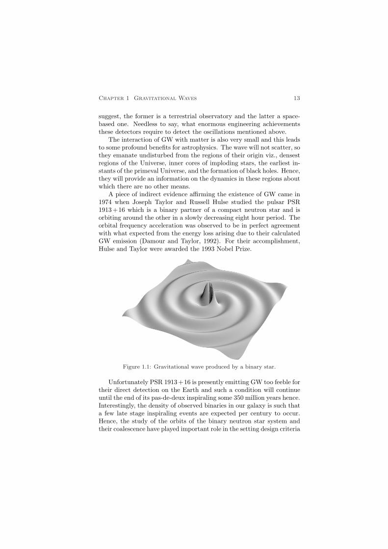
Gravitational waves (GW) like any other type of waves are propagatingperturbations of some flat background space-time. These are identifiedas small ripples rolling across space-time in the same manner as waterwaves are on an otherwise flat ocean. These waves originate from themost energetic events in our Universe such as rotating neutron stars,colliding binaries, supernovae explosions and gravitational collapse inblack holes. They manifest themselves as strains in space-time thatperiodically stretch and compress matter. The GW emanating from abinary may be represented as in Fig. (1.1).
Newtonian gravitation does not have the provision for GW. In sev-eral Lorentz covariant gravitational theories, e.g. scalar, vector, tensortheories, GW arise as the spreading out gravitational influence. Thebasis of most current thinking of GW is Einstein’s theory of GeneralRelativity (GR). In fact, GW phenomenon was first studied by Einsteinin 1916 by applying linear field approximation to GR. However, he wasmisled to the result that an accelerated spherical mass would emit GW.He corrected his mistake in 1918 and showed that the first order termof GW was quadrupolar.
The strength of GW is so small that there is no hope of its detec-tion in the manner Hertz demonstrated the existence of electromagneticwaves. The reason may be attributed to the extremely small value ofthe universal constant of gravitation (G ' 6.7×10⁻¹¹ Nm2kg−2). Thedimensionless amplitude of typical GW reaching the Earth is only of theorder of 10−17. This put in other words means that such a GW will puta rod of one meter length into an oscillation with an amplitude of onemillionth of the radius of a hydrogen atom. Any chance to observe theeffects of GW would require acceleration of astrophysical size massesat relativistic speeds. Several GW-detectors are running, or have beenproposed for the future, that hope to detect these very small vibrations.The best known of these are Laser Interferometer Ground Observatory(LIGO), and Laser Interferometer Space Antenna (LISA). As the names
Chapter 1 Gravitational Waves 13
suggest, the former is a terrestrial observatory and the latter a space-based one. Needless to say, what enormous engineering achievementsthese detectors require to detect the oscillations mentioned above.
The interaction of GW with matter is also very small and this leadsto some profound benefits for astrophysics. The wave will not scatter, sothey emanate undisturbed from the regions of their origin viz., densestregions of the Universe, inner cores of imploding stars, the earliest in-stants of the primeval Universe, and the formation of black holes. Hence,they will provide an information on the dynamics in these regions aboutwhich there are no other means.
A piece of indirect evidence affirming the existence of GW came in1974 when Joseph Taylor and Russell Hulse studied the pulsar PSR1913+16 which is a binary partner of a compact neutron star and isorbiting around the other in a slowly decreasing eight hour period. Theorbital frequency acceleration was observed to be in perfect agreementwith what expected from the energy loss arising due to their calculatedGW emission (Damour and Taylor, 1992). For their accomplishment,Hulse and Taylor were awarded the 1993 Nobel Prize.
Figure 1.1: Gravitational wave produced by a binary star.
Unfortunately PSR 1913 +16 is presently emitting GW too feeble fortheir direct detection on the Earth and such a condition will continueuntil the end of its pas-de-deux inspiraling some 350 million years hence.Interestingly, the density of observed binaries in our galaxy is such thata few late stage inspiraling events are expected per century to occur.Hence, the study of the orbits of the binary neutron star system andtheir coalescence have played important role in the setting design criteria
14 S. K. Sahay Data Analysis of Gravitational Waves
for some of the instruments to come into operation in the next few years.To the date we have only the indirect evidence of GW. Yet this has notbeen of much concern for theoretical physicists, because the strength ofthe postulated GW signals are below the detection threshold currentlyavailable.
The quest to detect GW started in its earnest as early as in 1965with the pioneering work of J. Weber on resonating bars. These arebasically high quality bells designed to be rung by transient GW. Withthis beginning a small GW detection community has arisen and thrivedcontinuing to improve on the original idea. The main effort is directedtowards noise reduction by introducing ever lower cryogenic tempera-ture and ever more sensitive displacement sensor to improve detectorsensitivity. Many more bars, progressively sophisticated ones, have beenbuilt. The Explorer which is quietly functioning at CERN since 1989,is one such detectors worth mention.
There is an excellent prospect of detection of GW in the near future.There will emerge what has been called “Gravitational Wave Astron-omy”. This will provide another window for observing the Universe.The expectation is that it will uncover new phenomena as well as addnew insights into phenomena already observed in electromagnetic partof the spectrum. GW emanation is due to the accelerated motions ofmass in the interior of objects. As remarked earlier, these regions areotherwise obscure in electromagnetic, and possibly, even in neutrinoastronomy. GW arise due to the coherent effects of masses moving to-gether rather than individual motions of smaller constituents such asatoms or charged particles which generate electromagnetic radiation.
§1.2 Einstein’s tensor
Gravitational waves like electromagnetic waves may be defined as timevarying gravitational fields in the absence of its sources. The gravitationtheory, widely believed, is the one proposed by Einstein and famous asGR. In its mathematical essence it is expressed via the equation knownby his name viz.∗
Gαβ = Rαβ − 12gαβ R = 8πTαβ . (1.1)
The conceptual meaning of this equation is that the localized densitydistribution characterized by the energy-momentum tensor, Tαβ , curvesthe space-time around the source. The curvature and other geometri-cal properties of the space-time are characterized by Ricci’s curvature
∗For notations, conventions and definitions the reader may refer to Schutz (1989).

Chapter 1 Gravitational Waves 15
tensor Rαβ and the underlying metric tensor gαβ . The curved space-time forces a free mass particle or light to follow the geodesics. Thesegeodesics measure the effect of gravitation. GR in the limit of a weakfield yields the Newton’s theory of gravitation. In this approximationthe gravitational field is considered to be represented by a metric witha linear modification of the background Lorentz space-time metric, ηαβ .It is important to remark that many of the basic concepts of GW the-ory can be understood in this approximation and were introduced anddeveloped by Einstein himself.
§1.3 Linear field approximation
The metric of the space-time may be expressed as
gαβ = ηαβ + hαβ , |hαβ | ¿ 1 . (1.2)
It is straight forward to compute Einstein’s tensor, Gαβ , and oneobtains
Gαβ = −12
[h , µ
αβ, µ + ηαβ h, µν
µν − h , µαµ, β − h , µ
βµ, α +O(h2
αβ
)], (1.3)
wherehαβ = hαβ − 1
2ηαβh , h = hα
α = − hαα . (1.4)
We lift and lower the tensor indices using the Lorentz metric. Notethat the expression for Gαβ would simplify considerably, if we wererequiring
hµν, ν = 0 . (1.5)
In fact there is a gauge freedom available as an infinitesimal coordi-nate transformation defined as
xα → x′α = xα + ξα (xβ) , |ξα| ¿ 1 , (1.6)
where ξα is taken arbitrary. This gauge transformation preserves (1.2).It can be shown that, in order to achieve the condition (1.5), ξα has tobe chosen as to satisfy
2 ξµ = ξµν, ν = h(old)µν
, ν , (1.7)
where the symbol 2 is used for the four-dimensional Laplacian:
2 f = f , µ, µ = ηµνf, µν =
(− ∂2
∂t2+52
)f . (1.8)
The gauge condition defined via (1.5) is called the Lorentz gauge.We adopt this gauge. In literature harmonic gauge and de Donder gauge
16 S. K. Sahay Data Analysis of Gravitational Waves
are other names for this gauge. Einstein’s tensor, to the first order inhαβ , becomes
Gαβ = −12
2 hαβ . (1.9)
Thus the weak-field Einstein equations take the form
2 hµν = −16πTµν . (1.10)
In the Newtonian limit, where the gravitational fields are too weakto produce velocities near the speed of light,
∣∣T00∣∣ À ∣∣T0j
∣∣ À ∣∣Tij∣∣ , T00 ' % , 22 ' 52. (1.11)
Equation (1.10) now results into
52h00 = −16π% . (1.12)
This equation may be compared to the Newtonian equation for grav-itational potential ϕ, i.e.
52ϕ = − 4π% . (1.13)
One obtains, after some calculations
h00 = 2ϕ , hxx = hyy = hzz = − 2ϕ , (1.14)
and accordingly the space-time metric for a Newtonian gravitationalfield is represented via
ds2 = −(1 + 2ϕ)dt2 + (1− 2ϕ)(dx2 + dy2 + dz2) . (1.15)
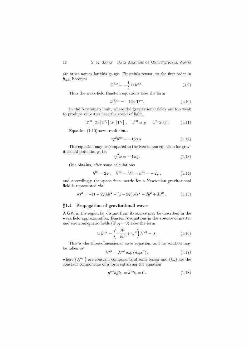
§1.4 Propagation of gravitational waves
A GW in the region far distant from its source may be described in theweak field approximation. Einstein’s equations in the absence of matterand electromagnetic fields (Tαβ = 0) take the form
2 hµν =(− ∂2
∂t2+52
)hαβ = 0 . (1.16)
This is the three-dimensional wave equation, and its solution maybe taken as
hαβ = Aαβ exp (ikγxγ) , (1.17)
whereAαβ
are constant components of some tensor and kα are the
constant components of a form satisfying the equation
ηµνkµkν = kνkν = 0 . (1.18)
Chapter 1 Gravitational Waves 17
This means that (1.17) represents a solution of (1.16) provided kγ isnull form and the associated four vector kα is null. The value of hαβ isconstant on a hyper-surface on which kαx
α is constant i.e.
kαxα = k0t+ k · x = const , k = ki . (1.19)
It is conventional to refer k0 as w, which is called the frequency ofthe wave
kα = w,k . (1.20)
The gauge condition (1.5) now requires
Aαβkβ = 0 , (1.21)
which means that Aαβ must be orthogonal to kβ .The solution (1.17) represents a plane wave propagating with the
velocity of light. In physical applications one has to consider the realpart of the solution.
Having the solution hαβ obtained, one still has the freedom of choos-ing specific ξα with the requirement that it represents some solution ofthe Eq. (1.7) which, in view of (1.16), becomes
(− ∂2
∂t2+52
)ξα = 0 . (1.22)
Take a solution of it as
ξα = Bα exp(ikµxµ) , (1.23)
where Bα is constant. It can be shown that the freedom available inchoosing the values of Bα may be employed such that the new Aαβ
satisfy the conditionsAα
α = 0 , (1.24)
AαβUβ = 0 , (1.25)
where Uα is some fixed four-velocity. Eqs. (1.21), (1.24), and (1.25) arecalled the transverse traceless (TT) gauge conditions. We choose Uα
as the time basis vector Uα = δα0. Let the direction of propagation
of the wave be the z-axis of the coordinate frame. Now using (1.18)and (1.20) we have kµ: (w, 0, 0, w). Now Eq. (1.25) in view of (1.21)implies: (i) Aα0 = 0, and (ii) Aαz = 0 for all α. This is the reason to callthe gauge “transverse gauge”. Further the trace free condition (1.24)requires Axx =−Ayy. Now the non-vanishing component of Aαβ may be

18 S. K. Sahay Data Analysis of Gravitational Waves
expressed as
ATTµν =
0 0 0 00 A+ A× 00 A× −A+ 00 0 0 0
; Axx = A+ , Axy = A× . (1.26)
Thus there are only two independent components of Aαβ , A+, andA×. Note that the traceless condition (1.24) results into
hTTαβ = hTT
αβ . (1.27)
We have considered the plane wave solution of Eq (1.16). We knowthat any solution of Eqs. (1.21) and (1.16) may be expressed, becauseof the theorems on Fourier analysis, as a superposition of plane waves.Hence if considering the waves propagating along z-axis, we can put allsuch planes waves into the form (1.27). Thus any wave has only twoindependent components hTT
xx and hTTxy represented, respectively, as h+
and h× corresponding to A+ and A×.
§1.5 The effect of waves on free particles and its polarization
The independent components h+ and h× represent the polarizationstates of the wave. To understand their nature in little detail it isinstructive to discuss the effect of a GW as it hits a free particle. Letus choose a background Lorentz frame where the particle is initially atrest. We may employ the initial four-velocity of the particle (Uα = δα
0)to define the TT gauge of the wave. A free particle obeys the geodesicequation
dUα
dτ+ Γα
µνUµUν = 0 . (1.28)
This geodesic equation may be used to obtain the initial accelerationof the particle
(dUα
dτ
)
t=0
= −Γα00 = − 1
2ηαβ (hβ0, 0 + h0β, 0 − h00, β) . (1.29)
In view of Eqs. (1.17, 1.26, 1.27), the initial acceleration of the parti-cle vanishes. This means that the particle will be at rest a instant laterand, consequently, will be there forever. What does it mean? Is thereno effect of a GW on a free particle? No, the interpretation presentedat its face value is quite misleading. The result only means that thechoice of the TT gauge employed resulted into a coordinate frame forthe wave which stays attached to the individual particles.
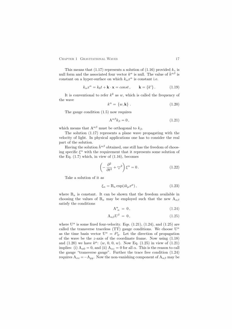
Chapter 1 Gravitational Waves 19
To get a better measure of the effect of the wave, we consider twonearby particles situated at the origin (0, 0, 0) and on the x-axis, (ε, 0, 0)separated by a distance ε. In view of the above discussion the parti-cles remain at their initial coordinate positions. The proper distancebetween them is
4l =∫ ∣∣ds2∣∣1/2
=∫ ∣∣gαβdx
αdxβ∣∣1/2
=∫ ε
0
|gxx|1/2dx ≈ |gxx(x = 0)|1/2
ε
4l =
1 +12hTT
xx (x = 0)ε . (1.30)
Thus the proper distance between two particles (as opposed to theircoordinate distance) does change with time. The effects of the wave mayalso be described in terms of the geodesic deviation of the separationvector, ηα, connecting these two particles. It obeys the equation
d2
dτ2ηα = Rα
µνβ UµUνηβ . (1.31)
It can be shown that for the particles initially having the separationvector, ηα → (0, ε, 0, 0), one would get
∂2
∂t2ηx =
12ε∂2
∂t2hTT
xx ,∂2
∂t2ηy =
12ε∂2
∂t2hTT
xy . (1.32)
Similarly, for initial separation vector, ηα → (0, 0, ε, 0) we would get
∂2
∂t2ηy =
12ε∂2
∂t2hTT
yy = −12ε∂2
∂t2hTT
xx
∂2
∂t2ηx =
12ε∂2
∂t2hTT
xy
. (1.33)
Note that, in view of the results of the previous §1.4 of this book,we may write (1.17) as
hαβ = Aαβ exp(wt− kz) . (1.34)
Thus the separation vector ηα of the particles oscillates.Consider a ring of particles initially resting in the (x, y) plane as
shown in Fig. (1.2-a). Suppose a wave having hTTxx 6= 0, hTT
xy = 0 hitsthe system of the particles. The particles will be moved (in terms ofthe proper distance relative to the one in the centre) in the way shownin Fig. (1.2-b). Similarly, for a wave with hTT
xx = 0 = hTTyy , h
TTxy 6= 0 the
picture would distort as in Fig. (1.2-c). Since hTTxx and hTT
xy are indepen-
20 S. K. Sahay Data Analysis of Gravitational Waves
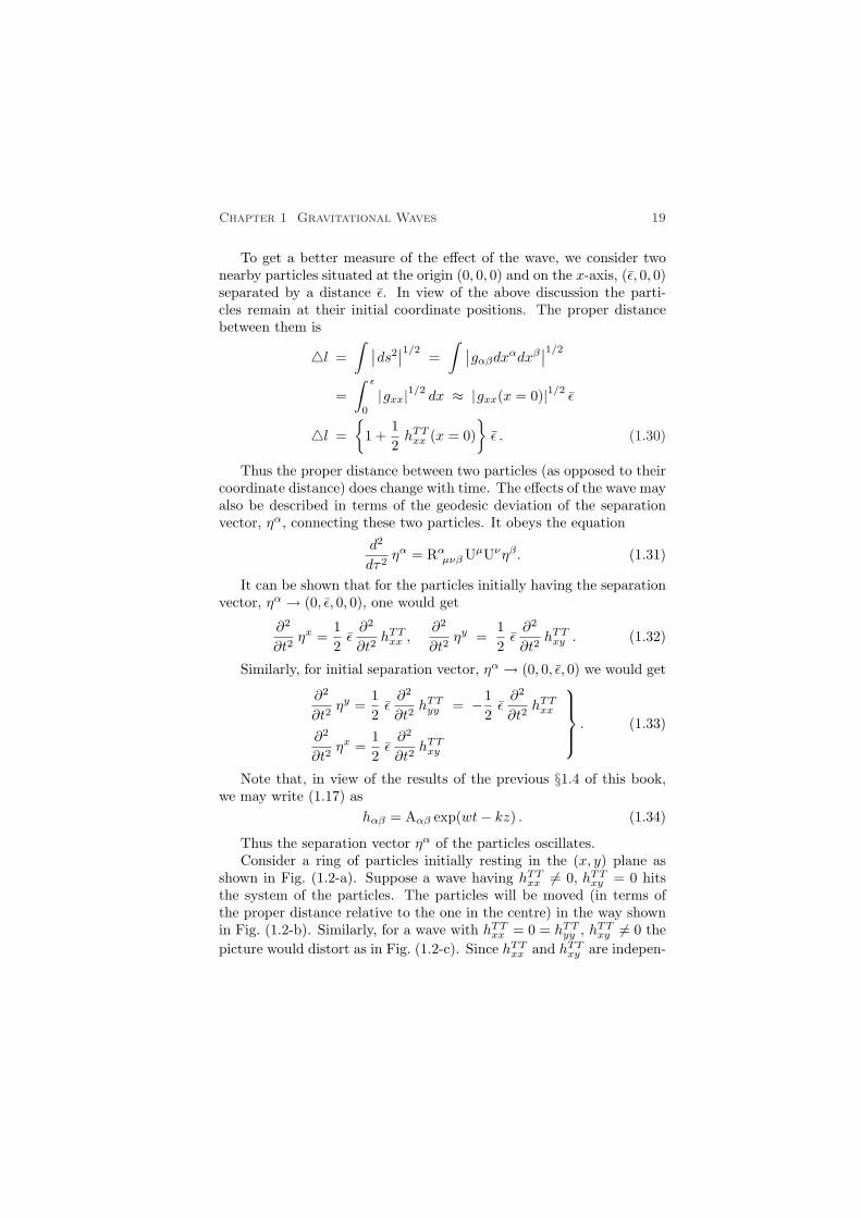
Figure 1.2: (a) A circle of free particles before a wave travelling in the zdirection reaches them. The (b) and (c) distortions of the circle are due toa wave with the “+” and “×” polarization. These two pictures representthe same wave at the phases separated by 180. The particles are positionedaccording to their proper distances from one another.
dent, Fig. (1.2-b) and (1.2-c) provide the pictorial representation of thepolarization states of the wave. Note that these two polarization statesare simply rotated by 45 relative to each other. This is in contrast toelectromagnetic waves where such two polarization states are at 90 toeach other.
§1.6 Generation of gravitational waves
To understand the generation of GW it is sufficient to discuss the weakfield limit Equation (1.10), rewritten as
(− ∂2
∂t2+52
)hµν = −16πTµν . (1.35)
We assume, for sake of simplicity, the time dependence of Tµν as aharmonic oscillation of an angular frequency ω, i.e.
Tµν = Sµν(xj)e−iωt , (1.36)
and look for a solution for hµν in the form
hµν = Bµν(xj)e−iωt . (1.37)

Chapter 1 Gravitational Waves 21
This, in view of Eqs. (1.35) and (1.36), would require Bµν to satisfy(52 + ω2
)Bµν = − 16πSµν . (1.38)
Outside the source, i.e. where Sµν = 0, we want a solution whichwould represent outgoing radiation far away. Hence we may take thesolution as
Bµν =(Aµν
r
)eiωr . (1.39)
Obviously, Aµν is to be related to Sµν . Under the assumption thatthe region of the space where Sµν 6= 0 is small compared to 2π
ω , it canbe deduced that
Aµν = 4Jµν ; Jµν =∫
Sµν d3x . (1.40)
This assumption is referred to as the slow motion approximationsince it implies that the typical velocity inside the source, which is ωtimes the size of that region, should be much less than 1. All, exceptthe most powerful sources, satisfy this assumption. Thus we get
hµν =(
4r
)Jµν e
iω(r−t) . (1.41)
This means that the generated GW has the frequency ω. This rela-tion may be expressed in terms of the useful quantities with the help ofthe following results:
(i) The energy-momentum satisfies the conservation equation
Tµν, ν = 0 , (1.42)
(ii) and obeys the identity
d2
dt2
∫T00 xlxmd3x = 2
∫Tlmd3x ; (1.43)
(iii) The quadrupole moment tensor Ilm is defined as
Ilm =∫
T00 xlxmd3x (1.44)
and which, in view of (1.36), may be expressed as
Ilm = Dlm e−iωt , (1.45)
where Dlm represents the time independent factor of Ilm (Misneret al., 1973).

22 S. K. Sahay Data Analysis of Gravitational Waves
The first result gives
Jµo = 0 ⇒ hµ0 , (1.46)
whereas the others let us write (1.41) as
hjk =(−2r
)ω2Djk e
iω(r−t) . (1.47)
We have still freedom of adopting TT gauge and may use it to achievefurther simplification. Let us choose the z-axis along the direction ofpropagation of the wave. We will then have
hTTzi = 0 , (1.48)
hTTxx = − hTT
yy = −ω2 (Ixx − Iyy)(eiωr
r
), (1.49)
hTTxy = −
(2r
)ω2 Ixy e
iωr , (1.50)
where Ijk represents the trace free part of the quadrupole moment ten-sor, i.e.
Ijk = Ijk − 13δjk Ii
i . (1.51)
As an application of our results we determine the amplitude of theGW generated by a laboratory source.
§1.6.1 Laboratory generator (bar)
Consider a system of two equal mass points capable to be oscillatingabout their mean position. Let the system oscillates longitudinally withan angular frequency w about its mean position, i.e.
x1 = − 12l0 −Acos wt
x2 =12l0 + A coswt
, (1.52)
where l0 is the normal separation between the mass points, and A repre-sents the amplitude of oscillation. Now it is straight forward to computeIjk. The only non-zero component is
Ixx = m[(x1)2 + (x2)2
]
= const+ mA2 cos 2wt+ 2ml0Acos wt . (1.53)

Chapter 1 Gravitational Waves 23
For purpose of wave generation the constant term is irrelevant. Wemay obtain the non-vanishing components of Ijk as
Ixx =43
m l0Ae−iwt +23
m l0A2 e−2iwt
Iyy = Izz = − 23
m l0Ae−iwt − 13
m l0A2 e−2iwt
. (1.54)
Finally one obtains, after taking the real part,
hTTxx = − hTT
xy = − [2mw2 l0A cos(w(r − t))
+ 4mw2A2 cos(2w(r − t))]/r
hTTxy = 0
. (1.55)
For a laboratory generator, we take
m = 103 kg , l0 = 1 m , A = 10−4 m , w = 10−4 s−1. (1.56)
The chosen data represent a typical bar detector. Substitutingthe values after converting them into geometrized units (G = 1 = c)the amplitude of the generated wave is about 10−34/r
|h | ' 10−34/r ; laboratory source. (1.57)
This manifests that laboratory generators are unlikely to produce auseful GW for its demonstration. For sake of comparison, we estimatethe strength of the waves produced by powerful astrophysical sources.
§1.6.2 Astrophysical sources
For a strong GW we should have hµν = O(1). This would occur neara source where the Newtonian potential would be of the order 1. For asource of a mass M, this should be at a distance of order M. As we haveseen the amplitude of a GW falls off as r−1 far distant from the source.This means that the largest amplitude expected to be incident on theEarth would be ∼ M/R, where R is the distance between the sourceand the Earth. For the formation of a 10 M¯ black hole in a supernovaexplosion in a nearby galaxy 1023 away, this is about 10−17. Thus
|h |max ' 10−17 ; astrophysical sources. (1.58)
Thus is in fact an upper limit and less violent events will lead tovery much smaller amplitudes.
Chapter 2
GRAVITATIONAL WAVE DETECTORS
§2.1 Introduction
The strain produced due to the hitting of a GW in two mass pointsseparated by ε is of the order of h. In view of Eq. (1.58) we note thateven a strong GW signal would produce a space strain of the orderof 10−17 that is an unbelievably small effect which would jerk massesspaced at one kilometer by a mere 10−20 — one thousand of the diameterof a proton!
Joseph Weber (1960) who pioneered the direct detection of GWconstructed an instrument consisting of a massive cylinder of aluminiumso-called “bar” detector. Such a detector exploit the sharp resonance ofthe cylinder to get its sensitivity which is normally confined to a narrowbandwidth (one or a few Hz) around the resonant frequency.
Despite their great potential sensitivity the primary drawback of res-onant bars is that they are by definition resonant. They are sensitivemainly to the signal with a frequency corresponding to the bar mechan-ical ringing frequency of the order of 1 kHz. A bar would respond tothe hammer blow of the asymmetrical supernova explosion by simplyringing at its own bell tones and would be excited by a twin neutronstar inspiraling only in that brief instant when these two stars crib upthrough the bell tone frequency.
Bar detectors continue to be developed, and they have until very re-cently had a sensitivity to broadband bursts. However, the best hope forthe first detection of GW lies with large-scale interferometers. Withinten years from now, we may see the launch of a space-based interfer-ometer, LISA, to search for signals at frequencies lower than those thatare not accessible from the ground. To measure the strain produced byGW to a bar or an interferometric detector, one must fight against thedifferent sources of noises.
An interesting additional twist is given by the fact that gravitationalwaves may be accompanied by gamma ray bursts. The GW detectorswill then work in coincidence not only with themselves and GW bar an-tennae, but also with conventional high-energy physics detectors like theunderground neutrino experiments and the orbital gamma rays burstmonitors.
Chapter 2 Gravitational Wave Detectors 25
§2.2 Bar detectors
A bar detector, in its simplest form, may be idealized as a system oftwo mass points coupled to a spring. Let the system lies on the x-axisof our TT coordinate frame with the masses at the coordinate positionsx1 and x2. The force free oscillation of the system, in the flat spacetime, may be expressed via
mx1, 00 = −κ(x1 − x2 + l0)− ν (x1 − x2) , 0
mx2, 00 = −κ(x2 − x1 + l0)− ν (x2 − x1) , 0
, (2.1)
where l0, κ, and ν represent respectively the outstretched length of thespring, spring constant, and damping constant. We can combine theseequations to obtain the usual damped harmonic oscillator equation
ξ, 00 + 2γ ξ, 0 + w20 ξ = 0 (2.2)
by introducing
ξ = x2 − x1 − l0 , w20 =
2κm, γ =
ν
m. (2.3)
We recall that the TT coordinate frame is not convenient for dis-cussion of the dynamics of such a system because in this frame a freeparticle always (before the arrival and after the passage of the wave)remains at rest. However this fact is useful in assigning a local inertialframe xα′ at some TT coordinate. Suppose that the only motions inthe system are those produced by the wave then masses velocities willbe very small so we may apply Newton’s equations of motion for themasses
mxj′
, 0′0′ = Fj′ , (2.4)
where Fj′ are the components of any non-gravitational forces on themass. Further as the coordinates xj′ differ negligibly to the order ofhµν from that of its value xj in TT coordinate frame, we may writethis equation with a negligible error
mxj, 00 = Fj . (2.5)
The only non-gravitational force on each mass is due to the spring.The spring exerts a force proportional to its instantaneous proper exten-sions. If the proper length of the spring is l and the direction of propa-gation of the wave, for simplicity, is assumed to be along the z-axis then
l (t) =∫ x2(t)
x1(t)
[1 + hTT
xx (t)]1/2
dx ≈[1 +
12hTT
xx (t)]
(x2 − x1) ; (2.6)
26 S. K. Sahay Data Analysis of Gravitational Waves
refer to (1.30). Hence, the equation of motion of the system after thehitting of the wave is given via
mx1, 00 = −κ(l0 − l)− ν (l0 − l) , 0
mx2, 00 = −κ(l − l0)− ν (l − l0) , 0
. (2.7)
Let us define
ξ = l − l0 =[1 +
12hTT
xx
](x2 − x1)− l0 , (2.8)
leading to
x2−x1 ' (ξ + l0)(
1− 12hTT
xx
)= ξ+ l0− 1
2hTT
xx l0 +O(|hµν |2
). (2.9)
Using this equation, we may obtain from Eq. (2.7)
ξ, 00 + 2γ ξ, 0 + w20 ξ =
12l0h
TTxx,00 (2.10)
correct to the first order in hTTxx .
This is the fundamental equation governing the response of the de-tector to a GW. It has the simple form of a forced, damped harmonicoscillator.
Let a GW of frequency ω described via
hTTxx = A cosωt (2.11)
be hitting the detector. Then the steady solution for ξ may be taken as
ξ = R cos (ωt+ ϕ)
R =12
l0ω2A
[(w0 − ω)2 + 4ω2ν2]1/2
tanϕ =2νω
w20 − ω2
. (2.12)
The average energy of the detector’s oscillation over one period, 2πω :
〈E〉 =18
mR2 (w20 + ω2) . (2.13)
If we wish to detect a specific source whose frequency ω is known,we should adjust w0 equal to ω for maximum response (resonance).

Chapter 2 Gravitational Wave Detectors 27
The resonance amplitude and energy of the detector will be
Rresonant =14l0A
ω
γ, (2.14)
Eresonant =164
m l20ω2A2
(ω
γ
)2
. (2.15)
The ratio ω/γ is related to what is called the quality factor Q.
Q =ω
2γ, (2.16)
Eresonant =116
m l20ω2A2Q2. (2.17)
The bar detectors are massive cylindrical bars; its elasticity providesthe function of the spring. When waves hit the bar broadside, theyexcite its longitudinal modes of vibration. The first detectors built byWeber were aluminium bars of the mass 1.4×10³ kg, length l0 =1.5 m,resonant frequency w0 = 104 s−1 and Q about 105. This means thata strong resonant GW of A = 10−20 will excite the bar to an energyof the order of 10−20 J. The resonant amplitude given by (2.14) is onlyabout 10−15 m, roughly the diameter of an atomic nucleus.
Figure 2.1: A schematic resonant bar detector.
Clearly, the detections of such small levels of excitations will behampered by random noise in the oscillator. For example, thermal noisein any oscillator induces random vibration with a mean energy of kT,where k is the Boltzmann constant having value 1.38×10⁻²³ J/K. Atroom temperature (T ∼ 300K) the thermal noise amounts to the energy∼ 4×10⁻²¹ J. Other sources of noise such as vibrations from passing

28 S. K. Sahay Data Analysis of Gravitational Waves
Detector Location Taking data since
NAUTILUS Frascati, Rome 1993
EXPLORER Cern (Rome group) 1990
ALLEGRO Louisiana, USA 1991
AURIGA Padua, Italy 1997
NIOBE Perth, Australia 1993
Table 2.1: Location of the resonant bar detectors.
vehicles and every day seismic disturbances could be considerably largerthan this, so the apparatus has to be carefully isolated.
A typical “bar” detector consists of an aluminium cylinder with alength l0 ∼ 3 m, a resonant frequency of order w0 ∼ 500 Hz to 1.5 kHz,and a mass ∼ 1000 kg whose mechanical oscillations are driven by GW;see Fig. (2.1). A transducer converts mechanical vibrations of the barinto an electrical signal, which is then amplified by an amplifier andrecorded.
Currently there are a number of bar detectors in operation; see Ta-ble (2.1). Some of these operate at room temperature and some others atcryogenic temperature. Some detectors (NAUTILUS and EXPLORER)may be cooled down to ultra cryogenic temperature. They can detectsignal amplitudes h ∼ 10−20 in a band width of 10–20 Hz around a cen-tral frequency of 1 kHz. Asymmetric supernovae in our Galaxy are thebest candidates for these detectors. For example, a supernova collapse inour galaxy at a distance of 10 kpc emits GW of the amplitude h∼ 10−17.At present this sensitivity has been achieved by some of the bar detec-tor. They may also see continuous radiation emitted by a neutron starif the frequency happens to lie in their sensitivity band.
§2.3 Ground-based laser interferometric detectors
The effect of GW is to produce a transverse shear strain and this factmakes the Michelson interferometer an obvious candidate for such adetector. The Michelson interferometers must have kilometric arms,constituted by “high fineness” Fabry Perot cavities to trap the lightfor long period and to increase the sensitivity. Laser standing powermeasured in KW will be stored within the cavities. Beam losses atthe level of 10−6 per passages are required. The mirrors must be 20
Chapter 2 Gravitational Wave Detectors 29
Detector
Locatio
nLength
(m)
Corner
Locatio
nA
rm
1A
rm
2
Gla
sgow
Gla
sgow
,G
BR
10
55.8
7 N
–4.2
8 W
77.0
0
167.0
0
CIT
Pasa
den
a,C
A,U
SA
40
34.1
7 N
–118.1
3 W
180.0
0
270.0
0
MP
QG
arc
hin
g,G
ER
30
48.2
4 N
–11.6
8 W
329.0
0
239.0
0
ISA
S-1
00
Tokyo,JP
N100
35.5
7 N
–139.4
7 W
42.0
0
135.0
0
TA
MA
-20
Tokyo,JP
N20
35.6
8 N
–139.5
4 W
45.0
0
315.0
0
Gla
sgow
Gla
sgow
,G
BR
10
55.8
7 N
–4.2
8 W
62.0
0
152.0
0
TA
MA
-300
Tokyo,JP
N300
35.6
8 N
–139.5
4 W
90.0
0
180.0
0
GE
O-6
00
Hannov
er,G
ER
600
52.2
5 N
–9.8
1 W
25.9
4
291.6
1
VIR
GO
Pis
a,IT
A3000
43.6
3 N
–10.5 W
71.5
0
341.5
0
LIG
OH
anfo
rd,W
A,U
SA
4000
46.4
5 N
–119.4
1 W
36.8
0
126.8
0
LIG
OLiv
ingst
on,LA
,U
SA
4000
30.5
6 N
–90.7
7 W
108.0
0
198.0
0
Table
2.2
:T
he
site
and
ori
enta
tion
ofth
egro
und-b
ase
din
terf
erom
etri
cgra
vit
ati
onalw
ave
det
ecto
rs.
30 S. K. Sahay Data Analysis of Gravitational Waves
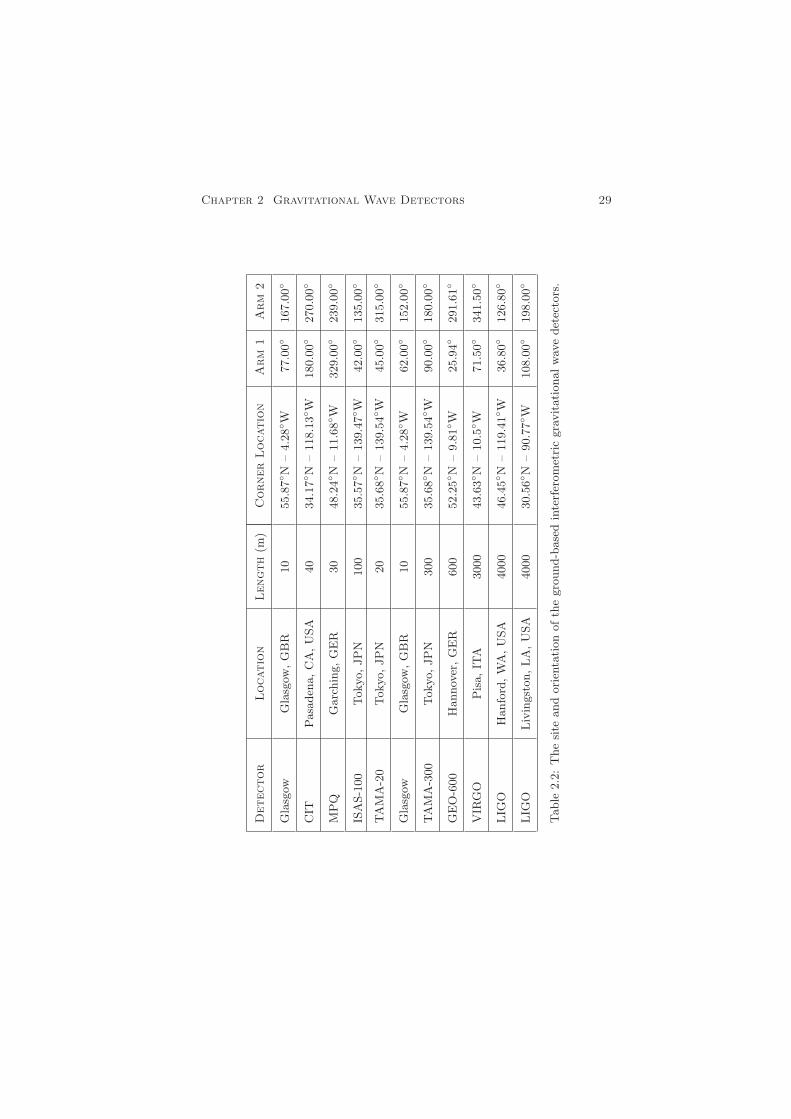
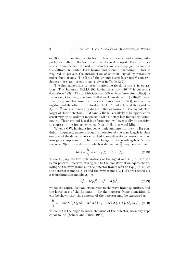
or 30 cm in diameter just to hold diffraction losses, and coating withparts per million reflection losses have been developed. Vacuum tubeswhose diameter is in the order of a meter are necessary just to containthe diffraction limited laser beams and vacuum exceeding 10 torr isrequired to prevent the introduction of spurious signal by refractionindex fluctuations. The list of the ground-based laser interferometricdetector sites and orientations is given in Table (2.2).
The first generation of laser interferometric detectors is in opera-tion. The Japanese TAMA-300 having sensitivity 10−20 is collectingdata since 1999. The British-German 600 m interferometer (GEO) inHannover, Germany, the French-Italian 3 km detector (VIRGO) nearPisa, Italy and the American two 4 km antennas (LIGO), one in Liv-ingston and the other in Hanford in the USA had achieved the sensitiv-ity 10−21 are also analyzing data for the signature of GW signal. Thelarger of these detectors, LIGO and VIRGO, are likely to be upgraded insensitivity by an order of magnitude with a better low-frequency perfor-mance. These ground based interferometers will eventually be sensitiveto sources in the frequency range from 10 Hz to several kHz.
When a GW, having a frequency high compared to the ∼ 1 Hz pen-dulum frequency, passes through a detector of the arm length l0 thenone arm of the detector gets stretched in one direction whereas the otherarm gets compressed. If the total change in the arm-length is δl, theresponse R(t) of the detector which is defined as δl
l0may be given via
R(t) =δl
l0= F+h+(t) + F×h×(t) , (2.18)
where h+, h× are two polarizations of the signal and F+, F× are thebeam pattern functions arising due to the transformation equations re-lating to the wave frame and the detector frame; refer to Eq. (1.31). Letthe detector frame (x, y, z) and the wave frame (X,Y, Z) are related viaa transformation matrix A, i.e.
ξi = AiRξ
R , ξk = Akj ξ
j , (2.19)
where the capital Roman letters refer to the wave frame quantities, andthe lower case of the Romans — for the detector frame quantities. Itcan be shown that the response of the detector may be expressed as
δl
l0= − sin 2Ω
[(Ax
XAyY −Ax
Y AyY )h++ (Ax
XAyY +Ax
Y AyX)h×
], (2.20)
where 2Ω is the angle between the arms of the detector, normally keptequal to 90 (Schutz and Tinto, 1987).
Chapter 2 Gravitational Wave Detectors 31
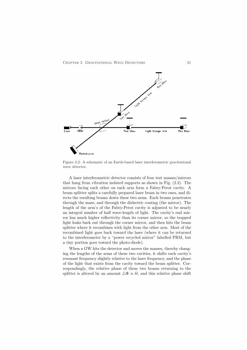
Figure 2.2: A schematic of an Earth-based laser interferometric gravitationalwave detector.
A laser interferometric detector consists of four test masses/mirrorsthat hang from vibration isolated supports as shown in Fig. (2.2). Themirrors facing each other on each arm form a Fabry-Perot cavity. Abeam splitter splits a carefully prepared laser beam in two ones, and di-rects the resulting beams down these two arms. Each beams penetratesthrough the mass, and through the dielectric coating (the mirror). Thelength of the arm’s of the Fabry-Perot cavity is adjusted to be nearlyan integral number of half wave-length of light. The cavity’s end mir-ror has much higher reflectivity than its corner mirror, so the trappedlight leaks back out through the corner mirror, and then hits the beamsplitter where it recombines with light from the other arm. Most of therecombined light goes back toward the laser (where it can be returnedto the interferometer by a “power recycled mirror” labelled PRM, buta tiny portion goes toward the photo-diode).
When a GW hits the detector and moves the masses, thereby chang-ing the lengths of the arms of these two cavities, it shifts each cavity’sresonant frequency slightly relative to the laser frequency, and the phaseof the light that exists from the cavity toward the beam splitter. Cor-respondingly, the relative phase of these two beams returning to thesplitter is altered by an amount 4Φ ∝ δl, and this relative phase shift
32 S. K. Sahay Data Analysis of Gravitational Waves
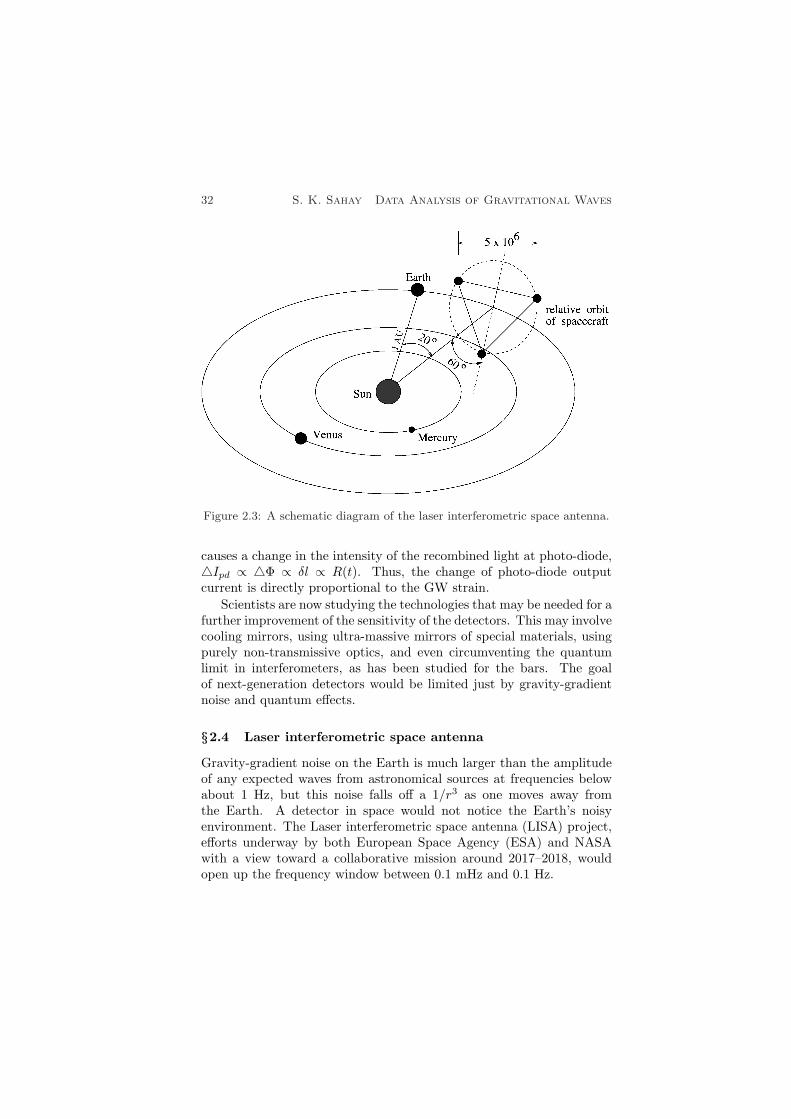
Figure 2.3: A schematic diagram of the laser interferometric space antenna.
causes a change in the intensity of the recombined light at photo-diode,4Ipd ∝ 4Φ ∝ δl ∝ R(t). Thus, the change of photo-diode outputcurrent is directly proportional to the GW strain.
Scientists are now studying the technologies that may be needed for afurther improvement of the sensitivity of the detectors. This may involvecooling mirrors, using ultra-massive mirrors of special materials, usingpurely non-transmissive optics, and even circumventing the quantumlimit in interferometers, as has been studied for the bars. The goalof next-generation detectors would be limited just by gravity-gradientnoise and quantum effects.
§2.4 Laser interferometric space antenna
Gravity-gradient noise on the Earth is much larger than the amplitudeof any expected waves from astronomical sources at frequencies belowabout 1 Hz, but this noise falls off a 1/r3 as one moves away fromthe Earth. A detector in space would not notice the Earth’s noisyenvironment. The Laser interferometric space antenna (LISA) project,efforts underway by both European Space Agency (ESA) and NASAwith a view toward a collaborative mission around 2017–2018, wouldopen up the frequency window between 0.1 mHz and 0.1 Hz.
Chapter 2 Gravitational Wave Detectors 33
A concept of the project is shown in Fig. (2.3). Three spacecraft areplaced in a solar orbit at 1 A.U., about 20 degrees behind the Earthin it orbit. The spacecrafts are located at the corners of an equilateraltriangle with 5×10⁶ km long sides. Two arms of the triangle comprisea Michelson interferometer with vertices at the corners. The third armpermits another interferometric observable to be measured, which candetermine a second polarization. The interferometers use one micronlight as the terrestrial detectors but need only a single pass in the armsto gain the desired sensitivity. The end points of the interferometers arereferenced to proof masses which are free-floating within and shieldedby the spacecraft. The spacecrafts are incorporated in a feedback loopwith precision thrust control to follow the proof masses.
The main environmental disturbances to LISA are the forces fromthe Sun: fluctuations in the solar radiation pressure and the pressuredue to the solar wind. To minimize these, LISA incorporates a drag-freetechnology. Interferometry is referenced to an internal proof mass thatfalls freely, not attached to the spacecraft. The job of the spacecraft is toshield this mass from external disturbances. It does this by sensing theposition of the mass and firing its own jets to keep itself (the spacecraft)stationary relative to the proof mass. To do this, it needs thrustersof very small thrust that have accurate control. The availability ofsuch thrusters, of the accelerometers needed to sense disturbances tothe spacecraft, and of the lasers capable of continuously emitting 1 Winfrared light for years, have enabled the LISA mission.
LISA is supposed to see many exciting sources for example the co-alescence of giant black holes in the centre of galaxies. LISA will seesuch events with extraordinary sensitivity, recording typical signal-to-noise-ratios of 1000 or more for events at redshift 1.
Chapter 3
SOURCES OF GRAVITATIONAL WAVES
§3.1 Introduction
Astronomical observations have led to the belief that luminous mat-ter constitutes a small fraction of the total matter content of the Uni-verse. More than 90% of the mass in the Universe is electro-magneticallysilent. The presence of dark matter is inferred from the gravitationalinfluence it causes on luminous matter. It is possible that some frac-tion of this dark matter is a strong emitter of GW. There are manyreviews on GW sources (Thorne, 1987; Blair, 1991; Schutz, 1989, 1993,1999; Sathyaprakash, 1999). The discussion on the GW sources in thisChapter is introductory and for details one may refer to these reviews.The anticipated GW sources can be classified into (i) transients, (ii)continuous, and (iii) stochastic.
§3.2 Supernovae explosions
The type II Supernovae explosions, which are believed to occur as a re-sult of the core collapse of an evolved massive (> 9M¯) star and whichare associated with violent mass ejection with velocities of order 0.03with formation of a compact remnant — a neutron star or a black hole— may emit significant amount of GW depending upon how asymmet-ric the collapse is. The emission occurs essentially during the rotationalcore collapse, bounce and oscillations, rotation-induced bars and con-vective instabilities set up in the core of the new born neutron star.
Rapid rotation flattens of the collapsing core induces a strong quad-rupole moment; thus generating GW. Study of a wide range of rotationalcore collapse models suggests that the largest signals are produced bymodels which are (i) initially slow rotating and have a stiff equation ofstate, or (ii) initially rapid rotating and have a soft equation of state.In the first case bounce occurs at densities above the nuclear matterdensity, with a fast deceleration of the collapsing core resulting in theemission of GW signals. In the second case, the quadrupole momentis strong due to the rapid rotation which facilitates the emission ofGW. However, in either case the signals are not strong enough to beinteresting sources for the first generation detectors.
Chapter 3 Sources of Gravitational Waves 35
When the core’s rotation is speedy enough , it may cause the coreto flatten before it reaches the nuclear density leading to an instabilitytransforming the flattened core into a bar-like configuration spinningabout its transverse axis. Some of these instabilities could also fragmentthe core into two or more pieces which then rotate about each other.Both are efficient ways of the losing energy in the form of GW.
Instabilities in the core of the newly born neutron star, which lastfor about a second after the collapse, are likely to produce GW due toanisotropic mass distribution and motion.
§3.3 Inspiraling compact binaries
The binary systems whose either member is a compact star e.g. a neu-tron star (NS) and a black hole (BH) are the most promising transientsources of GW during the phase of their coalescence. The well known bi-nary pulsar PSR 1913+16 is such a system but it will coalesce in a timescale of 109 years from now — not a right candidate. However, thereare binaries in our galaxy with coalescence time scale much shorter thanthis one. Further, statistical analysis of binary pulsars estimates threeNS-NS coalescence per year out to a distance of 200 Mpc (Phinney, 1991;Narayanan et al. 1991). The initial LIGO/VIRGO interferometers havea fair chances to see the inspiral events. Compact inspiraling binariesemit quasi-periodic GW with a frequency that sweeps upward toward amaximum frequency. The maximum frequency may be of the order of 1KHz for neutron stars. In the lower frequency regime the wave form iseasily computed from the quadrupole formalism. At higher frequenciespost-Newtonian corrections would be required (Thorne, 1987; Krolak,1989). In view of the strong potentialities of such sources the variousaspects related to the emission of GW has been dealt extensively in fulldetails, and one may refer to Sathyprakash (1999).
§3.4 Continuous gravitational wave
Continuous gravitational wave (CGW) sources are of our prime inter-est because such sources can be observed again and again and hencesingle interferometer is sufficient to confirm its detection. However, onecan’t expect a continuous source to be strong. For emission of GWfrom pulsars, there should be some asymmetry in it. There are severalmechanisms which may lead to deformations of the star, or to precessionof its rotation axis. The characteristic amplitude of GW from pulsarsscales as
h ∼ If20 ε
r, (3.1)

36 S. K. Sahay Data Analysis of Gravitational Waves
where I is the moment of inertia of the pulsar, f0 is the GW frequency,ε is a measure of deviation from axissymmetry, and r is the distancebetween the detector and the pulsar.
As remarked earlier, pulsars are born in supernovae explosions. Theouter layers of the star crystallizes as the newborn star pulsar cools byneutrino emission. Estimates, based on the expected breaking strain ofthe crystal lattice, suggest that anisotropic stresses, which build up asthe pulsar looses rotational energy, could lead to ε 6 10−5; the exactvalue depends on the breaking strain of the neutron star crust as wellas the neutron star’s “geological history”, and could be several ordersof magnitude smaller. Nonetheless, this upper limit makes pulsars apotentially interesting source for kilometer scale interferometers.
Large magnetic fields trapped inside the super fluid interior of apulsar may also induce deformation of the star. This mechanism hasbeen explored recently, indicating that the effect is extremely small forstandard neutron star models (ε 6 10−9).
Another plausible mechanism for CGW is the Chandrasekhar-Friedman-Schutz (CFS) instability, which is driven by GW back re-action. It is possible that newly-formed neutron stars may undergothis instability spontaneously as they cool soon after formation. Thefrequency of the emitted wave is determined by the frequency of theunstable normal mode, which may be less than the spin frequency.
Accretion is another way to excite neutron stars. There is also theZimmermann-Szedinits mechanism where the principal axes of the mo-ment of inertia are driven away from the rotational axes by accretionfrom a companion star. Accretion can in principle produce a relativelystrong wave since the amplitude is related to the accretion rate ratherthan to structural effects in the star.
§3.5 Stochastic waves
Catastrophic processes in the early history of Universe, as well as the as-trophysical sources distributed all over the cosmos, generate stochasticbackground of GW. A given stochastic background will be characteristicof the sources that are responsible for it and it may be possible to dis-criminate different backgrounds provided their spectral characteristicsare sufficiently different.
Primordial background: It is believed that similar to cosmic mi-crowave background (CMBR) a GW background was also produced atthe same time as a result of quantum fluctuations in the early Universe(Grischuk, 1997). Primordial background radiation would freely travel

Chapter 3 Sources of Gravitational Waves 37
to us from almost the very moment of the creation because GW couplesvery weakly with matter. Hence, its detection would help us in the get-ting a picture of the first moments after the big bang. The COBE datahave set limits on the strength of the GW background. The strengthare far too weak to be detected by any running ground-based detectors.However, advanced LIGO detectors may observe the background gen-erated by the collisions of a cosmic string network (for details one mayrefer to Allen, 1997).
Phase transitions in the early Universe, inspired by fundamentalparticle physics theories, and cosmological strings and domain wallsare also sources of a stochastic background. These processes are ex-pected to generate a background which has a different spectrum andstrength than the primordial one. Future ground-based detectors willachieve good enough sensitivity to measure this background GW andsuch measurements will prove to be a good test bed for these cosmolog-ical models.
Supernovae background: Even though an individual supernova maynot be detectable out to a great distance, the background produced byall supernovae within the Hubble radius might indeed be detected (Blairand Ju, 1996). The coincidence between an advanced interferometer anda resonant bar within 50 km of the interferometer will enable the detec-tion of this background. These studies may shed light on the history ofstar formation rate, a subject of vigorous debate amongst astrophysi-cists.
Galactic binary background: Binaries with orbital periods P ∼10−4−10−2 s will be observable in space-based detectors. A large num-ber of them are present in our galaxy but they will not be identifiableseparately because they are at a large distances and consequently havea feeble amplitude. However they would contribute to background GW.In addition to binaries of compact stars, there are also other binariesconsisting of white dwarfs, cataclysmic variables, etc., which will alsocontribute to the background radiation produced by compact binaries.The net effect is that these sources will appear as a background noise inspace interferometers. By studying the nature of this background onecan learn a lot about binary population in our Galaxy.
Galactic pulsar background: CGW from pulsars could also producea background of GW radiation which will limit the sensitivity of theground-based laser interferometers (Giazotto, Gourgoulhon, and Bonaz-zola, 1997). There are about 109 neutron stars in our Galaxy of which
38 S. K. Sahay Data Analysis of Gravitational Waves
about 2×10⁵ will contribute to the background radiation. This back-ground radiation will be prominent and observable in the LIGO/VIRGOdetectors, in the frequency range of 5–10 Hz, at an rms amplitude ofhrms ∼ 2×10⁻²⁶, where the rms is computed over 105 sources. At fre-quency of 10 Hz, the wavelength of GW will be around 30,000 km.Hence, it would be possible to cross-correlate data from two distant de-tectors, such as two LIGOs, or LIGO and VIRGO, and discriminate thebackground against other sources of noise.

Chapter 4
DATA ANALYSIS CONCEPT
§4.1 Introduction
The GW data analysis strategy is different in many ways from conven-tional astronomical data analysis. This is due to the following:
• GW antennae are essentially omni-directional with their responsebetter than 50% of the average over 75% of the sky. Hence ourdata analysis systems will have to carry out all-sky searches forthe sources;
• Interferometers are typically broad-band covering 3 to 4 orders ofmagnitude in the frequency. While this is obviously to our ad-vantage, as it helps to track sources whose frequency may changerapidly, it calls for searches to be carried over a wide-band offrequencies;
• In contrast to electromagnetic (EM) radiation, most astrophysicalGWs are tracked in the phase, and the signal-to-noise ratio (SNR)is built up by coherent superposition of many wave cycles emittedby a source. Consequently, the SNR is proportional to the ampli-tude and only falls off, with the distance to the source, r, as 1/r.Therefore, the number of sources of a limiting SNR increases as r3
for a homogeneous distribution of the sources in a flat Universe,as opposed to EM sources that increase only as r3/2;
• GW antennae acquire data continuously for many years at therate of several mega-bytes per second. It is expected that about ahundredth of this data will have to pass through our search analy-sis systems. Unless on-line processing can be done we cannot hopeto make our searches. This places huge demands on the speed ofour data analysis hardware. A careful study of our search algo-rithms with a view to making them as optimal (maximum SNR)and efficient (least search times) as one possibly can is required.
§4.2 Gravitational wave antenna sensitivity
The performance of a GW detector is characterized by the one sidedpower spectral density (PSD) of its noise background. The analytical fits
40 S. K. Sahay Data Analysis of Gravitational Waves
to noise power spectral densities Sn(f) of ground based interferometersare given in Table (4.2), where S0 and fn0 represent respectively thevalue of the minimum noise and the corresponding frequency. At thelower-frequency cutoff fl and the high-frequency cutoff fu, Sn(f) canbe treated as infinite. One can construct the noise PSD as follows.
A GW detector output represents a dimensionless data train, sayx(t). In the absence of any GW signal the detector output is just aninstance of noise n(t), that is, x(t) = n(t). The noise auto-correlationfunction c is defined as
c(t1, t2) ≡ 〈n(t1)n(t2)〉, (4.1)
where 〈 〉 represents the average over an ensemble of the noise realiza-tions. In general, c depends on both t1 and t2. However, if the detectoroutput is a stationary noise process, i.e. its performance is, statisticallyspeaking, independent from time, c depends only on τ ≡ t2 − t1. Weshall, furthermore, assume that c(τ) = c(−τ). For data from real de-tectors the above average can be replaced by a time average under theassumption of ergodicity:
c(τ) =1T
∫ T/2
−T/2
n(t)n(t− τ) dt . (4.2)
The assumption of stationarity is not strictly valid in the case of realGW detectors; however, if their performance does not vary greatly overtime scales much larger than typical observation time scales, stationaritycould be used as a working rule. While this may be good enough inthe case of binary inspiral and coalescence searches, it is a matter ofconcern for the observation of continuous and stochastic GW. Undersuch an assumption the one-sided noise PSD, defined only at positivefrequencies, is the Fourier Transform (FT) of the noise auto-correlationfunction:
Sn(f) ≡ 12
∫ ∞
−∞c(τ)e−2πifτ dτ, f > 0 ,
≡ 0 , f < 0 , (4.3)
where a factor of 12
is included by convention because it has been as-sumed that c(τ) is an even function. This equation implies that Sn(f)is real. It is straightforward to show that
〈n(f) n∗(f ′)〉 = Sn(f) δ (f − f ′) , (4.4)
where n(f) represents the Fourier transform of n(t) and ∗ denotes com-plex conjugation. This identity implies that Sn(f) is positive definite.

Chapter 4 Data Analysis Concept 41
Detector
Fit
to
nois
epow
er
spectral
densi
ty
S0
(Hz)−
1f n
0(H
z)f l
(Hz)
f u(H
z)
LIG
OI
S0 3
" „f n
0
f
« 4+
2
„f f n
0
« 2#
8.0×
10−
46
175
40
1300
LIG
OII
S0
11
( 2
„f n
0
f
« 9/2
+9 2
" 1+
„f f n
0
« 2#)
7.9×
10−
48
110
25
900
LIG
OII
IS
0 5
( „f n
0
f
« 4+
2
" 1+
„f
fn
0
« 2#)
2.3×
10−
48
75
12
625
VIR
GO
S0 4
" 290
„f s f
« 5+
2
„f n
0
f
«+
1+
„f fn0
« 2#
1.1×
10−
45
475
16
2750
GE
O600
S0 5
" 4
„f n
0
f
« 3/2
−2
+3
„f f n
0
« 2#
6.6×
10−
45
210
40
1450
TA
MA
S0
32
( „f n
0
f
« 5+
13
„f n
0
f
«+
9
" 1+
„f f n
0
« 2#)
2.4×
10−
44
400
75
3400
Table
4.1
:A
naly
tica
lfits
tonois
epow
ersp
ectr
alden
siti
esS
n(f
)ofth
egro
und-b
ase
din
terf
erom
eter
s.

42 S. K. Sahay Data Analysis of Gravitational Waves
The autocorrelation function c(τ) at τ = 0 can be expressed as anintegral over Sn(f). Indeed, it is easy to see that
〈n2(t)〉 = 2∫ ∞
0
Sn(f)df . (4.5)
The above equation justifies the name power spectral density givento Sn(f). It is obvious that Sn(f) has a dimension of time but it isconventional to use, instead, a dimension of Hz−1 since it is a quantitydefined in the frequency domain. The square-root of Sn(f) is the noiseamplitude,
√Sn(f), and has a dimension of per root Hz. It is often
useful to define the dimensionless quantity h2n(f) ≡ fSn(f) called the
effective noise. In GW interferometer literature one also comes acrossthe displacement noise or strain noise defined as hl0(f) ≡ l0hn(f), andthe corresponding noise spectrum Sl0(f) ≡ l20Sn(f), where l0 is the armlength of the interferometer. The displacement noise gives the smalleststrain δl/l0 in the arms of an interferometer which can be measured ata given frequency.
§4.2.1 Sensitivity vs source amplitudes
One compares the GW amplitudes of astronomical sources with theinstrumental sensitivity and assesses what sort of sources will be ob-servable in the following way. First, as comparisons are almost alwaysmade in the frequency-domain, it is important to note that the Fouriercomponent h(f) of a deterministic signal h(t) has a dimension of Hz−1
and the quantity f | h(f)| is dimensionless. It is the last quantity thatshould be compared with hn(f) to deduce the strength of a source rel-ative to the detector noise. Second, it is quite common also to comparethe amplitude spectrum per logarithmic bin of a source,
√f | h(f)|, with
the amplitude spectrum of the noise,√Sn(f), both of which have di-
mensions of per root Hz. For monochromatic sources, one comparesthe effective noise in a long integration period with the expected “in-stantaneous” amplitudes in the following way: a monotonic wave of afrequency f0 observed for a time T0 is simply a narrow line in a fre-quency bin of width ∆f ≡ 1/T0 around f0. The noise in this bin isSn(f)∆f = Sn(f)/T0. Thus the SNR after a period of observation T0 is
S
N=
h0√Sn(f0)/T0
. (4.6)
One, therefore, computes this dimensionless noise spectrum fora given duration of observation, Sn(f)/T0, to assess the detectabilityof a continuous GW. Surely, if the observation time is T0 then the total
Chapter 4 Data Analysis Concept 43
energy (that is, the integrated power spectrum) of both signal and noisemust increase in proportion to T 2
0 . Then how does the SNR for a con-tinuous wave improve with the duration of observation? The point isthat while the signal energy is all concentrated in one bin, the noiseis distributed over the entire frequency band. As T0 increases, the fre-quency resolution improves as 1/T0 and the number of the frequencybins increases in proportion to T0. Consequently, the noise intensity perfrequency bin increases only as T0. Now, the signal intensity is concen-trated in just one bin since the signal is assumed to be monochromatic.Therefore, the power SNR increases as T0, or, the amplitude SNR in-creases as
√T0.
§4.3 Noises in the Earth-based interferometric detectors
As mentioned in the earlier section the performance of GW detectoris characterized by the one-sided PSD. The sensitivity of ground-baseddetectors is limited at frequencies less than a Hertz by the time-varyinglocal gravitational field caused by a variety of different noise sources, e.g.low frequency seismic vibrations, density variation in the atmospheredue to winds, etc. Thus, for data analysis purposes, the noise PSD isassumed to be essentially infinite below a certain lower cutoff fs. Theeffective noise hn(f) expected in these detectors is equal to
√fSn(f).
Type of noises that one have to fight to detect the signals are:Ground vibration: External mechanical vibrations are a problem forbar detectors, too, but are more serious for interferometers, not leastbecause interferometers bounce light back and forth between the mir-rors, and so each reflection introduces further vibrational noise. Sus-pension/isolation systems are based on pendula. A pendulum is a goodmechanical filter for frequencies above its natural frequency. By hangingthe mirrors on pendula of perhaps 0.5 m length, one achieves filteringbelow a few Hz. Since the spectrum of ground noise falls at higherfrequencies, this provides suitable isolation. But these systems can bevery sophisticated; the GEO600 detector has a three-stage pendulumand other vibration isolation components. Among all the ground basedlaser interferometer detectors, VIRGO has the best isolation system.Thermal noise: Vibrations of the mirrors and of the suspending pen-dulum can mask gravitational waves. As with vibrational noise, this isincreased by the bouncing of the light between the mirrors. Unlike bars,interferometers process measurements only at the frequencies which arefar from the resonant frequency, where the amplitude of vibration issmaller. Thus, the pendulum suspensions have thermal noises at a few
44 S. K. Sahay Data Analysis of Gravitational Waves
Hz, but measurements were performed at above 20 or 30 Hz in the firstdetectors. Internal vibrations of the mirrors have natural frequenciesof several kilohertz. By ensuring that both kinds of oscillations havevery high Q, one can confine most of the vibration energy to a smallbandwidth around the resonant frequency, so that at the measurementfrequencies the vibration amplitudes are small. This allows interferom-eters to operate at room temperature. But mechanical Qs of 107 orhigher are required, and this is technically demanding.
Shot noise: The photons that are used to do interferometry are quan-tized, so they arrive at random and make random fluctuations in thelight intensity that can look like a gravitational wave signal. The morephotons one uses, the smoother will be the interference signal. As arandom process, the error improves with the square-root of the numberN of photons. Using infrared light with a wavelength λ∼ 1µm, one canexpect to measure to an accuracy of
4Lshot ∼ λ
2π√
N.
To perform measurement at a frequency f , one has to make at least2f measurements per second i.e. one can accumulate photons for a time12f . With light power P and GW amplitude h one gets N= P
(hc/λ)(2f)
photons. In order that 4Lshot be below 10−16 m, one needs strong lightpower far beyond the output of any continuous laser.
Light-recycling techniques overcome this problem by using light ef-ficiently. An interferometer actually has two places where light leaves.One is where the interference is measured. The other goes back towardsthe input laser. Normally one arranges that no light goes to the inter-ference sensor, so that only when a gravitational wave passes makes asignal registered there. This means that all the light normally returnsto the mirror, apart from small losses at the mirrors. Since mirrors areof good quality, only one part in 103 or less of the light is lost during a1 ms storage time. By placing a power-recycling mirror in front of thelaser, one can reflect this wasted light back in, allowing power to buildup in the arms until the laser merely resupplies the mirror losses. Thiscan dramatically reduce the power requirement for the laser.
Quantum effects: Shot noise is a quantum noise, but in additionthere are effects like bar detectors face: zero-point vibrations of mirrorsurfaces and so on. These are small compared to present operatinglimits of detectors, but they may become important in 5 years or so.Practical schemes to reduce this noise have already been demonstrated

Chapter 4 Data Analysis Concept 45
in principle, but they need to be improved considerably. They canbe reduced by making the mirror masses large, since the amplitude ofvibration scales inversely as the square-root of the mass.
Gravity gradient noise: One noise which cannot be screened out isthat arises due to changes in the local Newtonian gravitational field onthe time scale of the measurements. A gravitational wave detector willrespond to tidal forces from local sources just as well as to gravitationalwaves. Environmental noise comes not only from man-made sources,but even more importantly from natural ones: seismic waves are accom-panied by changes in the gravitational field, and changes in air pressureare accompanied by changes in air density. The spectrum falls steeplywith increasing frequency. Hence, the running interferometers does nothave problem, but it may limit the performance of detectors a decadefrom now. And it is the primary reason that detecting gravitationalwaves in the low-frequency band around 1 mHz must be done in space.
§4.4 Matched Filtering and optimal signal-to-noise ratio
Matched Filtering is a data analysis technique that efficiently searchesfor a signal of known shape buried in the noisy data (Helstrom, 1968).The technique consists in correlating the noisy output of each inter-ferometer data with a set of theoretical waveform templates. If themaximum of the correlation exceeds a preset threshold, a detection isannounced. However, even if a signal is present in the data, the ac-companying noise can mask its presence by preventing such crossing ofthe threshold in some cases. Thus a signal can be detected with onlya certain probability called the detection probability. Also there willbe a non-zero probability called the false alarm probability, of a falsedetection due to noise alone. A formalism to choose the optimal set oftemplates using a criterion was first given by Sathyaprakash and Dhu-randhar (1991), and Dhurandhar and Sathyaprakash (1994) known asthe S-D formalism.
These search templates will be discrete subset of a continuous, multiparameter family, each of which approximate a possible signal. Givena signal h(t) buried in a noise n(t), the task is to find an “optimal” tem-plate q(t) that would produce, on the average, the best possible SNR.The enhancement in the signal-to-noise ratio not only increases the num-ber of detectable events but, more importantly, it also allows a more ac-curate determination of signal parameters — the error in the estimationof parameter being inversely proportional to the signal-to-noise ratio.
If the functional form of the template is identical to that of the sig-
46 S. K. Sahay Data Analysis of Gravitational Waves
nal, the mean signal-to-noise ratio in the presence of a signal is highestof the possible for any linear data processing technique, which is whymatched filtering is also known as optimal filtering (Helstrom, 1968).A matched filter , in the frequency domain, is a best-guess template ofthe expected signal waveform divided by the interferometer’s spectralnoise density.
In order to take full advantage of matched filtering it is essentialthat the phase of the waveform shall be known to a very high degree ofaccuracy to accumulate the SNR (Cutler et al., 1993). This is referred toas coherent integration of the signal, where the SNR grows
√T0. This is
in contrast to incoherent methods, such as stacking and tracking (Bradyet al., 1998, 2000), where one disregards the phase information and theSNR does not accumulate as quickly. Tracking involves tracking oflines in the time-frequency plane built from the FT of short (around 40minutes long) stretches of data. The other stacking involves dividing thedata into shorter (around a day long) stretches, searching each stretchfor signals, and enhancing the detectability by incoherently summingthe FT of data stretches.
There are several questions that must be answered in order to deter-mine the feasibility of a matched filtering search strategy and, if feasible,to implement it. Which parameters significantly affect the wave form?How should the spacing of the template parameters (lattice points) bechosen? Is there a parametrization that is in some sense preferred bythe template waveforms? How many templates are needed to cover agiven region of interest in the parameter space and how much computingpower and memory will it cost to process the data through them? In thecase of a modulated pulsar signal we must also ask what approximationto the true wave form is good enough?
Ambiguity function, well known in the statistical theory of signaldetection (Helstrom, 1968), is a very powerful tool in signal analysis. Ithelps to access the number of templates required to span the parameterspace of the signal. However, Apostolatos (1995) defined a term calledFitting Factor (FF ) which quantitatively describes the closeness of thetrue signals to the template manifold in terms of the reduction in SNRdue to cross correlation of a signal outside the manifold with all thetemplates lying inside the manifold.
§4.4.1 Fitting factor
One of the standard measurements for deciding what class of wave formis good enough is the Fitting Factor and has already been used by
Chapter 4 Data Analysis Concept 47
various authors∗ as a measure of adequateness of a template family,but previous discussions have not shown explicitly how this intuitivelywell-formed function is connected with detectability.
Previously FF has sometimes been called the “correlation”, a num-ber that is often used in so many different ways. The name comes fromthe fact that, by maximizing the quantity FF, the parameters of thetemplates can be adjusted to best fit of the true waveform.
Consider a detector receiving almost monochromatic GW signalsfrom a pulsar. The signal will be Doppler modulated due to the motionof the Earth and stars, represented by the function S(t). The outputX(t) of the detector will be
X(t) = S(t) + n(t) . (4.7)
If the search template is the exact waveform h(t), we achieve thehighest possible signal-to-noise ratio given as
(S
N
)
max
= 〈S(f)|S(f)〉2. (4.8)
where the inner product of two waveforms 〈h1|h2〉 is defined as
〈h1|h2〉 = 2∫ ∞
0
h∗1(f) h2(f) + h1(f) h∗2(f)Sn(f)
df
= 4∫ ∞
0
h∗1(f) h2(f)Sn(f)
df . (4.9)
The SNR ratio will be reduced below (S/N)max whenever the tem-plate is not the exact waveform but some other approximate one. Inthe case where the search is performed with some family of templatesST (f ; ~ξ) for a signal vector ~ξ (the signal is considered as a vector in theparametric space), then the SNR is given by
(S
N
)=
max
~ξ〈X(f)|ST (f ; ~ξ)〉rms〈n|ST (f ; ~ξ)〉
. (4.10)
For an ensemble of realizations of the detector noise, the expec-tation values 〈n|ST (f ; ~ξ)〉 and 〈n|ST (f ; ~ξ)〉〈n|ST (f ; ~ξ)〉 are zero, and〈ST (f ; ~ξ)|ST (f ; ~ξ)〉, respectively. Thus the ensemble-averaged signal-to-noise ratio turns out to be
∗Sathyaprakash and Dhurandhar (1991), Dhurandhar and Sathyaprakash (1994).

48 S. K. Sahay Data Analysis of Gravitational Waves
(S
N
)=
max
~ξ〈S(f)|ST (f ; ~ξ)〉√〈ST (f ; ~ξ)|ST (f ; ~ξ)〉
=
max
~ξ〈S(f)|ST (f ; ~ξ)〉√
〈ST (f ; ~ξ)|ST (f ; ~ξ)〉〈S(f)|S(f)〉
(S
N
)
max
. (4.11)
The name Fitting Factor is given to the reduction in signal-to-noiseratio that results because of using the chosen template family, ratherthan the true signal h, in the search:
FF (~ξ) =max
~ξ〈S(f)|ST (f ; ~ξ)〉√〈ST (f ; ~ξ)|ST (f ; ~ξ)〉
=max
~ξ〈S(f)|ST (f ; ~ξ)〉√
〈ST (f ; ~ξ)|ST (f ; ~ξ)〉〈S(f)|S(f)〉. (4.12)
Therefore, if the family of search template used at the detectionstage does not contain the true signal waveform, the reduction in thesignal-to-noise ratio will be given by
(S
N
)= FF (~ξ)×
(S
N
)
max
(4.13)
The spacing of the grid of filters is decided by the fractional loss dueto the imperfect match that can be tolerated. Given the parametersspace that one needs to scan, it is then easy to estimate the total num-ber of filters required to carry out the search for the signal. The signalstrength scales is inverse with distance, the fraction of event rate re-tained is approximately FF 3. Therefore it has become conventional toregard FF = 0.9 as the lowest acceptable FF value for some templatefamily to be considered adequate. A reduction in SNR by 10% means a27% loss in the event rate. On the other hand a 10% reduction in SNRis equivalent to a roughly 10% shortening of the detectors arms.
§4.5 Computational costs
Matched Filtering places stringent demands on the knowledge of thesignal’s phase evolution which depends on two things: (i) our modellingof the signal, and (ii) the parameters characterizing the signal. If oursignal model is inaccurate or if the signal’s parameters are unknown,there could be a loss in the SNR extracted. For instance, in the case of

Chapter 4 Data Analysis Concept 49
inspiral signals, a mismatch of one cycle in 104 cycles leads to a dropin the SNR by more than a factor of two, losing a factor of eight inthe number of potentially detectable events. Recall that the SNR isinversely proportional to the distance to a source; thus an SNR lossby a factor “a” will reduce the span of a detector by the same factor,resulting a decrease in the volume of observation, and hence the numberof events, by a factor a3. Moreover, since the parameters of a signalwill not be known in advance, it is necessary to filter the data with afamily of templates located at various points in the parameter spacee.g., placed on a lattice such that any signal will lie close enough to atleast one of the templates to have a good cross-correlation with thattemplate. The number of such templates is typically very large. Thisplaces a great demand on the computational resources needed to makean on-line search.
The search problem for continuous waves from spinning neutronstars is the most computer-intensive job in gravitational wave data anal-ysis. Today, there is little hope that all-sky searches lasting for a yearor more can be made. It is easy to see why this is such an intensive job:first, the data has to be collected continuously for months together andat a good sensitivity; second, though a neutron star emits a periodicsignal in its rest frame, save for the neutron star spin-down which in-deed induces some modulation in the waveform, because of the Earth’sacceleration relative to the source, the detector does not see a periodicwave. The wave is both frequency and amplitude modulated. One can,fortunately, de-modulate these effects since the Earth’s motion is knownquite accurately, and hence recover the original periodic signal. But de-modulation requires a knowledge about the source’s direction and itsfrequency, which are unknown in a blind search. The angular resolutionone obtains in a year’s integration is ∆θ = λ/D, where λ is the wavelength of radiation and D is the baseline of the detector in a year’s in-tegration, namely 1 A.U. Thus, for f = 1 kHz we have ∆θ = 10−6 rador about two arcsec. Now, assuming that the source may be in any oneof the 4 arcsec2 patches on the sky we get the number of patches inthe sky for which we will have to try out a de-modulation correction tobe 4π/(∆θ)2 = 4π×1012. It is a quite impossible task to apply Dopplerde-modulation to the detector output for each of these ∼ 1013 pathsand compute as many Fourier transforms.
One, therefore, asks a question: given a compute power what is thebest possible search one can do? Is there any advantage in going from aone-step search to a two or multi-step hierarchical search? What aboutdirectional searches? These are some of the problems for which we have
50 S. K. Sahay Data Analysis of Gravitational Waves
some answer; but a great deal of work is needed and is currently underprogress, to improve and optimize search algorithms.
The differential geometric studies shows that with a TFLOPS-classcomputer, the number of days of data can be analyzed on-line and wecan carry out a blind search. Unfortunately, the longest data we canintegrate on-line for neutron stars with spin frequencies f 6 100 Hz andspin-down rates less than 1000 years is about 18 days. This yields aSNR lower by a factor of 5 as compared to a year’s worth of observ-ing. On-line searches for neutron stars with f 6 500 Hz (the largestobserved frequencies of millisecond pulsars) and spin-down rates of 40years (shortest observed spin-down rates) can only be made for a dataset lasting for a duration of 20 hours or less. If source’s position isknown in advance, but not its frequency, then one can carry out an on-line search, again with a TFLOPS-class computer, for the frequency ofthe source in a data set that is worth 3 months long. This is good newssince there are many known pulsars and X-ray binary systems that arepotential sources of radiation. In addition, the obvious targeted searchlocations are the centre of the Galaxy and globular clusters.
There have been efforts to study the effectualness of a two-step hi-erarchical method for a blind search. Here the basic idea is to constructFourier transforms of data sets of duration smaller than the period inwhich Doppler modulations will be important and to stack spectral den-sities obtained in this way and to add them all up. This is an incoherentway of building the signal since one adds spectral densities that haveno phase information. Therefore, one gains in SNR less than whatan optimal matched filtering method is able to achieve. However, thisdoes not matter since (i) the targeted SNR’s are quite high ∼ 10, and(ii) candidate events can always be followed-up using coherent integra-tion methods. These methods afford an on-line all-sky blind search forcontinuous gravitational waves for a period of 4 months or less using a20 GFLOPS computer.
§4.6 Detection criteria
A signal needs to be above the noise experienced in the instrumentand environment. However, this alone is insufficient to establish it asa gravitational wave in the terrestrial detectors. The most satisfyingcircumstance is that a gravitational wave observation be made in a setof widely distributed detectors (the Gravitational Wave Network, orGWN in short) and the resorted wave forms allow the solutions forthe polarization of the wave and the position of the source. Armed
Chapter 4 Data Analysis Concept 51
with this information an electromagnetic (or neutrino) search could beattempted in the error circle of the gravitational wave detection: a timehonoured approach bringing gravitational wave of observation into themain stream of Astrophysics. The strategy would apply to all classes ofsources: impulsive chirps, quasiperiodic and periodic.
The confident detection of impulsive sources is most difficult, whilethe periodic and quasiperiodic detection will have confidence limitsbased on quasi-stationary system noise (the signals last long enough totake a meaningful sample of the noise spectrum), the impulsive signalsespecially if rare, will be particularly dependent of the non-Gaussiancomponent of the noise; the noise most difficult to reduce and controlin a signal detectors. The technique of multiple coincidence of severaldetectors is one of the best means to gain confidence. The coincidencemust occur within a time window to permit a consistent solution for a lo-cation in the sky. If the general character of the source can be guessedin advance (for example, a binary coalescence chirp, or a black-holenormal mode oscillation), the signal is filtered prior to the coincidencemeasurement to improve the sensitivity. The more detectors involved,the greater the confidence assigned to the detection.
There is still a possibility of coincidence due to environmental oranthropogenic causes. The various sites throughout the world are farenough apart that most environmental perturbations should not cor-relate between them. The acoustic noise, the seismic noise, and thepower line (especially if the network includes detectors in a differentpower grids and significantly different time zones) will be uncorrelated.There are correlations in the magnetic field fluctuations (thunderstorms)and in radio frequency emissions. As part of the detection strategy alarge number of environmental parameters will be measured along withthe gravitational wave signals at each site. One of the requirementsfor the authenticity of impulsive sources will be the lack of correlationwith environmental perturbations and other ancillary internal signalsdeveloped to monitor the performance of the instruments.

Chapter 5
DATA ANALYSIS — PART I
§5.1 Introduction
The first generation of long-baseline laser interferometers and ultra cryo-genic bar detectors is in operation. The network of detectors will notonly confirm the existence of GWs but will also yield an informationabout their important parameters viz; amplitude, frequency and phase.In addition, a careful monitoring of the signal will also provide an in-formation about the structure and dynamics of their source. The dataanalysis depends largely upon the study of the expected characteris-tic of the potential sources and the waveforms. The most part of theexperimental searches is focused on the detection of burst and chirpsignals. However, the interest in the data analysis for CGW signals isgrowing up. A prime example of the sources of GW signals of this typeis a spinning neutron star. Many research groups around the globe areworking extensively on the data analysis for spinning neutron stars; seeJaranwoski et al. (1998, 1999, 2000), Brady et al. (1998, 2000).
Our Galaxy is expected to have, on logistic grounds, at least 108
spinning neutron stars, with a birth rate of one per every 30 years. How-ever, a very insignificant fraction of them is observed — the number ofknown pulsars has gone up to ∼ 1600. There are compelling argumentsthat nearby millisecond pulsars can provide a detectable source of CGW.Hence, there is a strong case for scanning all the sky for the presenceof neutron stars with the philosophy that they are emitting GWs butotherwise unknown optically. This study will help us to understand thepulsar population in our Galaxy.
The detection of GW signals in the output has its own problems, notthe least of which is the sheer volume of data analysis. Bar detectorshave essentially the same problems as interferometers in the referenceto CGW sources. The possibility that these detectors are capable tosearch for signals of different kinds makes them very versatile, but alsocomplicates the data analysis. Each detector produces a single datastream that may contain many kinds of signals. Detectors don’t point,but rather sweep their broad quadrupolar beam pattern across the skyas the Earth moves. So possible sources could be anywhere on the sky
Chapter 5 Data Analysis — Part I 53
and accordingly the data analysis algorithms need to accommodate thesignals from any arbitrary location of its source.
In this Chapter and the next Chapter we analyze the FT of theoutput data of a ground-based laser interferometer. The output datahas prominently dominant broad band noise and the signal is to beextracted out of it. For this, one has to enhance SNR. This is achieved byanalyzing a long observation time data as SNR is directly proportionalto the square root of the observation time
√T0. However, in a data for
long duration, the monochromatic signal gets Doppler modulated dueto: (i) the orbital motions of the Earth around the Sun, and (ii) the spinof the Earth. The Frequency Modulation (FM) will spread the signal ina very large number of bins depending on the source location and thefrequency. In addition to it there is the Amplitude Modulation (AM).As we will see in the sequel the amplitude of the detector output consistsof simple harmonic terms with frequencies wrot and 2wrot, where wrot
stands for the angular rotational frequency of the Earth. Accordingly,the AM results in splitting of FT into frequencies ±wrot and ±2wrot.
§5.2 The noise free response of detector: beam pattern andamplitude modulation
Let a plane GW falls on a laser interferometer, and produces changesin the arms of the detector. In order to express these changes quan-titatively we would require to specify the wave and the detector. LetXY Z and xyz represent respective frames characterizing the wave andthe detector. We assume the direction of propagation of the wave to bethe Z-axis, and the vertical at the place of detector to be the z-axis.Proceeding from §2.3 of Chapter 2, the difference of the changes δl inthe arm lengths of the detector is given via
R(t) =δl
l0= − sin 2Ω [(Ax
XAyX −Ax
Y AyY )h+
+ (AxXAy
Y + AxY Ay
X)h×] , (5.1)
where l0 is the normal length of the arms of the detector, and 2Ω ex-presses the angle between them (Schutz and Tinto, 1987). The matrix(Aj
K
)represents the transformation expressing the rotations to bring
the wave frame (X,Y, Z) to the detector frame (x, y, z). The directionof the source may be expressed in any of the coordinates employed inspherical astronomy. However, we find it convenient to define it in theSolar System Barycentre (SSB) frame (X ′, Y ′, Z ′). This SSB frame isnothing but astronomer’s ecliptic coordinate frame. Let θ and φ denote
54 S. K. Sahay Data Analysis of Gravitational Waves
the celestial co-latitude and the celestial longitude of the source. Thesecoordinates are related to the right ascension α and the declination δ ofthe source via
cos θ = sin δ cos ε− cos δ sin ε sin α
sin θ cosφ = cos δ cos α
sin θ sinφ = sin δ sin ε+ cos δ cos ε sin α
, (5.2)
where ε represents the obliquity of the ecliptic. We choose the x-axisas the bisector of the angle between the arms of the detector. At thisstage the orientation of the detector in the horizontal plane is arbitrary.It is assigned with the help of the angle γ which the x-axis makes withthe local meridian.
The location of the detector on the Earth is characterized by theangle α, the co-latitude and the β, the local sidereal time expressed inradians. The transformation matrix
(Aj
K
)may be expressed as
A = DCB , (5.3)
where we introduced the following denotations:
B : a rotation required to bring XY Z to X ′Y ′Z ′;C : a rotation required to bring X ′Y ′Z ′ to x′y′z′;D : a rotation required to bring x′y′z′ to xyz.
Here x′y′z′ represents the frame associated with the Earth. TheEuler angles defining the corresponding rotation matrices (Goldstein,1980) are given via
B : (θ, φ, ψ)
C : (0, ε, 0)
D : (α, β + π2 , γ − π
2 )
, (5.4)
where ψ is a measure of the polarization of the wave. Let us expressEq. (5.1) as
R(t) =δl
l0= − sin 2Ω [F+h+ + F×h×] . (5.5)
The functions F+ and F× involve the angles θ, φ, ψ, ε, α, β, γ andexpress the effect of the interaction between the wave and the detector.These are called antenna or beam patterns. After a straight forwardcalculation one obtains Eqs. (5.6) and (5.7); see Jotania and Dhurand-har (1994) for detail. The next two pages of this book provide theseequations written in complete form.
Chapter 5 Data Analysis — Part I 55
F+(t) =12
[(cosψ cosφ− cos θ sinφ sinψ)2 − (cosψ sinφ+ cos θ cosφ sinψ)2
× 2(cosα cosβ cos γ − sinβ sin γ)(− cosα cosβ sin γ − sinβ cos γ)+
(− sinψ cosφ− cos θ sinφ cosψ)2 − (cos θ cosφ cosψ − sinψ sinφ)2
× [cos2 ε 2(cosα sinβ cos γ + cosβ sin γ)(cosβ cos γ − cosα sinβ sin γ)
− sin2 ε sin2 α sin 2γ + sin 2ε (cosα sinβ cos γ + cosβ sin γ) sinα sin γ
− (cosβ cos γ − cosα sinβ sin γ) sinα cos γ]− (sin2 θ cos 2φ)
× [sin2 ε 2(cosα sinβ cos γ + cosβ sin γ)(cosβ cos γ − cosα sinβ sin γ)
− cos2 ε sin2 α sin 2γ − sin 2ε (cosα sinβ cos γ + cosβ sin γ) sinα sin γ
− (cosβ cos γ − cosα sinβ sin γ) sinα cos γ]]+ (cosψ cosφ− cos θ sinφ sinψ)(− sinψ cosφ− cos θ sinφ cosψ)
− (cosψ sinφ+ cos θ cosφ sinψ)(cos θ cosφ cosψ − sinψ sinφ)× [cos ε (cosβ cos γ − cosα sinβ sin γ)(cosα cosβ cos γ − sinβ sin γ)
− (cosα sinβ cos γ + cosβ sin γ)(cosα cosβ sin γ + sinβ cos γ)+ sin ε (cosα cosβ cos γ − sinβ sin γ)(sinα sin γ)
+ (cosα cosβ sin γ + sinβ cos γ)(sinα cos γ)]+ (cosψ cosφ− cos θ sinφ sinψ)(sin θ sinφ)
+ (cosψ sinφ+ cos θ cosφ sinψ)(sin θ cosφ)× [− sin ε (cosβ cos γ − cosα sinβ sin γ)(cosα cosβ cos γ − sinβ sin γ)
− (cosα sinβ cos γ + cosβ sin γ)(cosα cosβ sin γ + sinβ cos γ)+ cos ε (cosα cosβ cos γ − sinβ sin γ)(sinα sin γ)
+ (cosα cosβ sin γ + sinβ cos γ)(sinα cos γ]+ (− sinψ cosφ− cos θ sinφ cosψ)(sin θ sinφ)
+ (cos θ cosφ cosψ − sinψ sinφ)(sin θ cosφ)× [−(cos ε sin ε) 2(cosα sinβ cos γ + cosβ sin γ)
× (cosβ cos γ − cosα sinβ sin γ) + sin2 α sin 2γ
+ cos 2ε (cosα sinβ cos γ + cosβ sin γ)(sinα sin γ)
− (cosβ cos γ − cosα sinβ sin γ)(sinα cos γ)] (5.6)
56 S. K. Sahay Data Analysis of Gravitational Waves
F×(t) = 2(cosψ cosφ− cos θ sinφ sinψ)(cosψ sinφ+ cos θ cosφ sinψ)
× (cosα cosβ cos γ − sinβ sin γ)(− cosα cosβ sin γ − sinβ cos γ)
+ (− sinψ cosφ− cos θ sinφ cosψ)(cos θ cosφ cosψ − sinψ sinφ)
× [cos2 ε 2(cosα sinβ cos γ + cosβ sin γ)(cosβ cos γ − cosα sinβ sin γ)
− sin2 ε sin2 α sin 2γ + sin 2ε (cosα sinβ cos γ + cosβ sin γ) sinα sin γ
− (cosβ cos γ − cosα sinβ sin γ) sinα cos γ]
− 12(sin2 θ sin 2φ)
× [sin2 ε 2(cosα sinβ cos γ + cosβ sin γ)(cosβ cos γ − cosα sinβ sin γ)
− cos2 ε sin2 α sin 2γ − sin 2ε (cosα sinβ cos γ + cosβ sin γ) sinα sin γ
− (cosβ cos γ − cosα sinβ sin γ) sinα cos γ]+ (cosψ cosφ− cos θ sinφ sinψ)(− sinψ sinφ+ cos θ cosφ cosψ)
− (cosψ sinφ+ cos θ cosφ sinψ)(cos θ sinφ cosψ + sinψ cosφ)× [cos ε (cosβ cos γ − cosα sinβ sin γ)(cosα cosβ cos γ − sinβ sin γ)
− (cosα sinβ cos γ + cosβ sin γ)(cosα cosβ sin γ + sinβ cos γ)+ sin ε (cosα cosβ cos γ − sinβ sin γ)(sinα sin γ)
+ (cosα cosβ sin γ + sinβ cos γ)(sinα cos γ)]+ −(cosψ cosφ− cos θ sinφ sinψ)(sin θ cosφ)
+ (cosψ cosφ+ cos θ cosφ sinψ)(sin θ sinφ)× [− sin ε (cosβ cos γ − cosα sinβ sin γ)(cosα cosβ cos γ − sinβ sin γ)
− (cosα sinβ cos γ + cosβ sin γ)(cosα cosβ sin γ + sinβ cos γ)+ cos ε (cosα cosβ cos γ − sinβ sin γ)(sinα sin γ)
+ (cosα cosβ sin γ + sinβ cos γ)(sinα cos γ]+ (− sinψ sinφ+ cos θ cosφ cosψ)(sin θ sinφ)
+ (cos θ sinφ cosψ + sinψ cosφ)(sin θ cosφ)× [−(cos ε sin ε) 2(cosα sinβ cos γ + cosβ sin γ)
× (cosβ cos γ − cosα sinβ sin γ) + sin2 α sin 2γ
+ cos 2ε (cosα sinβ cos γ + cosβ sin γ)(sinα sin γ)
− (cosβ cos γ − cosα sinβ sin γ)(sinα cos γ)] (5.7)

Chapter 5 Data Analysis — Part I 57
It is easy to understand the structure of the above complicated look-ing expressions for F+ and F× by introducing following abbreviations
U = cosα cosβ cos γ − sinβ sin γ
V = − cosα cosβ sin γ − sinβ cos γ
X = cosα sinβ cos γ + cosβ sin γ
Y = − cosα sinβ sin γ + cosβ cos γ
, (5.8)
L = cosψ cosφ− cos θ sinφ sinψ
M = cosψ sinφ+ cos θ cosφ sinψ
N = − sinψ cosφ− cos θ sinφ cosψ
P = − sinψ sinφ+ cos θ cosφ cosψ
Q = sin θ sinφ , R = sin θ cosφ
, (5.9)
A = 2XY cos2 ε− sin2ε sin2α sin 2γ
+ sin 2ε (X sinα sin γ − Y sinα cos γ)
B = 2XY sin2ε− cos2ε sin2α sin 2γ
− sin 2ε (X sinα sin γ − Y sinα cos γ)
C = cos ε (Y U +XV )
+ sin ε (U sinα sin γ − V sinα cos γ)
D = − sin ε (Y U +XV )
+ cos ε (U sinα sin γ − V sinα cos γ)
E = − 2XY cos ε sin ε− cos ε sin ε sin2α sin 2γ
+ cos 2ε (X sinα sin γ − Y sinα cos γ)
. (5.10)
One obtains:
F+(t) =12[2(L2 −M2)UV + (N2 − P 2)A + (Q2 −R2)B
]
+(LN −MP )C + (LQ+MR)D + (NQ+ PR)E , (5.11)
F×(t) = 2LMUV +NPA− 12B sin2θ sin 2φ
+(LP +MN)C + (MQ− LR)D + (PQ−NR)E . (5.12)
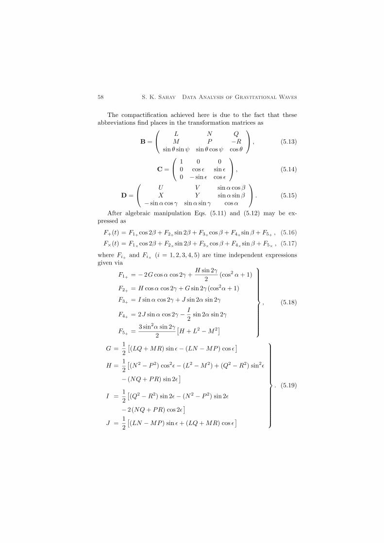
58 S. K. Sahay Data Analysis of Gravitational Waves
The compactification achieved here is due to the fact that theseabbreviations find places in the transformation matrices as
B =
L N QM P −R
sin θ sinψ sin θ cosψ cos θ
, (5.13)
C =
1 0 00 cos ε sin ε0 − sin ε cos ε
, (5.14)
D =
U V sinα cosβX Y sinα sinβ
− sinα cos γ sinα sin γ cosα
. (5.15)
After algebraic manipulation Eqs. (5.11) and (5.12) may be ex-pressed as
F+(t) = F1+cos 2β + F2+sin 2β + F3+cosβ + F4+sinβ + F5+ , (5.16)
F×(t) = F1×cos 2β + F2×sin 2β + F3×cosβ + F4×sinβ + F5× , (5.17)
where Fi+ and Fi× (i = 1, 2, 3, 4, 5) are time independent expressionsgiven via
F1+ = − 2G cosα cos 2γ +H sin 2γ
2(cos2 α+ 1)
F2+ = H cosα cos 2γ +G sin 2γ (cos2α+ 1)
F3+ = I sinα cos 2γ + J sin 2α sin 2γ
F4+ = 2J sinα cos 2γ − I
2sin 2α sin 2γ
F5+ =3 sin2α sin 2γ
2[H + L2 −M2
]
, (5.18)
G =12
[(LQ+MR) sin ε− (LN −MP ) cos ε
]
H =12
[(N2 − P 2) cos2ε− (L2 −M2) + (Q2 −R2) sin2ε
− (NQ+ PR) sin 2ε]
I =12
[(Q2 −R2) sin 2ε− (N2 − P 2) sin 2ε
− 2(NQ+ PR) cos 2ε]
J =12
[(LN −MP ) sin ε+ (LQ+MR) cos ε
]
. (5.19)

Chapter 5 Data Analysis — Part I 59
Note that Fi× is related to Fi+ via
Fi×(θ, φ, ψ, α, β, γ, ε
)= Fi+
(θ, φ− π
4 , ψ, α, β, γ, ε), (5.20)
where i=1, 2, 3, 4, 5.This symmetry represents the quadrupolar nature of the detector
and the wave. A detector in different orientations will record differentamplitudes in the response. The explicit beam pattern functions maybe computed easily for any instant of time. Due to symmetries involvedin F+ and F×, it is sufficient to discuss either of the beam patterns.
The amplitude modulation of the received signal is a direct conse-quence of the non-uniformity of the sensitivity pattern. The antennaresponse is not peaked in any direction but is anisotropic. As remarkedearlier they are fairly complicated function of their arguments. Equa-tions (5.16) and (5.17) reveal that the monochromatic signal frequencywill split, due to AM, into five lines. This results in the distributionof energy in various frequencies and consequent reduction of the ampli-tude of the signal. The periodicity of the beam patterns F+ and F×with a period equal to one sidereal day is due to the diurnal motion ofthe Earth.
§5.3 Doppler shift and frequency modulation
The frequency of a monochromatic signal will be Doppler shifted dueto the translatory motion of the detector, acquired from the motions ofthe Earth. Let us consider a CGW signal of a constant frequency f0.The frequency f ′ received at an instant t by the detector is given by
f ′(t) = f0γ0
(1 +
v · nc
(t)), γ0 =
(1− v2
c2
)−1/2
, (5.21)
where n is the unit vector from the antenna to the source, v is therelative velocity of the source and the antenna, and c is the velocityof light. The unit vector n from the antenna to the source, because ofthe fact that the distance of the source is very large compared to theaverage distance of the centre of the SSB frame and the detector, maybe taken parallel to the unit vector drawn from the centre of the SSBframe to the source. Hence,
n =(sin θ cosφ , sin θ sinφ , cos θ
). (5.22)
As v keeps on changing continuously in its both amplitude and di-rection, f ′ is a continuous function of t. Further, since v ¿ c we takeinto account that γ0 = 1.

60 S. K. Sahay Data Analysis of Gravitational Waves
The radius vector r(t) in the SSB frame is given, in componentnotation, by
r(t)=[Rse cos(worb t) +Re sinα cosβ ,
Rse sin(worb t) +Re sinα sinβ cos ε−Re cosα sin ε ,
Re sinα sinβ sin ε+Re cosα cos ε]; (5.23)
β = β0 + wrot t , (5.24)
where Re, Rse, and worb represent respectively the Earth’s radius, theaverage distance between the Earth’s centre from the centre of SSBframe, and the orbital angular velocity of the Earth. Here, t repre-sents the time in seconds elapsed from the instant Sun is at the VernalEquinox and β0 is the local sidereal time at that instant. The Dopplershift is now given via
f ′ − f0f0
=v · nc
(t) =rt · nc
=Rseworb
csin θ sin(φ− worb t)
+Rewrot
csinα
[sin θ
(cosβ cos ε sinφ− cosφ sinβ
)
+ cosβ sin ε cos θ]. (5.25)
The phase Φ(t) of the received signal is given by
Φ(t) = 2π∫ t
0
f ′(t′) dt′ = 2πf0∫ t
0
[1 +
v · nc
(t′)]dt′. (5.26)
Here, we assume the initial phase of the wave to be zero. After astraight forward calculation we obtain
Φ(t) = 2πf0
t+
Rse
csin θ cosφ′
+Re
csinα
[sin θ
(sinβ cos ε sinφ+ cosφ cosβ
)
+ sinβ sin ε cos θ]− Rse
csin θ cosφ
− Re
csinα
[sin θ
(sinβ0 cos ε sinφ+ cosφ cosβ0
)
+ sinβ0 sin ε cos θ]
= 2πf0t+Z cos(worb t−φ)+P sin(wrott)+Q cos(wrot t)−R−Q= 2πf0t+Z cos (a ξrot−φ)+N cos (ξrot−δ)−R−Q , (5.27)

Chapter 5 Data Analysis — Part I 61
where
P = 2πf0Re
csinα
[cosβ0 ( sin θ cos ε sinφ+ cos θ sin ε)
− sinβ0 sin θ cosφ]
Q = 2πf0Re
csinα
[sinβ0 ( sin θ cos ε sinφ+ cos θ sin ε)
+ cosβ0 sin θ cosφ]
N =√P2 +Q2
Z = 2πf0Rse
csin θ
R = Z cosφ
, (5.28)
δ = tan−1 PQ
φ′ = worbt− φ
ξorb = worbt = a ξrot; a = worb/wrot ≈ 1/365.26
ξrot = wrot t
. (5.29)
These two polarization states of the signal can be taken as
h+(t) = h0+ cos[Φ(t)
], (5.30)
h×(t) = h0× sin[Φ(t)
], (5.31)
where h0+ and h0× are the time independent amplitude of h+(t), andh×(t) respectively.
To understand the nature of the FM, let us consider the FT of h+(t)and h×(t). We may begin by considering the function
h(t) = cos[Φ(t)
](5.32)
and analyzing the data for one day observation. The FT is given via
[h(f)
]d
=∫ T
0
cos[Φ(t)
]e−i2πft dt , (5.33)
where T is one sidereal day, 86164 sec.This may be split into two terms as
[h(f)
]d
= Iν− + Iν+ ; (5.34)

62 S. K. Sahay Data Analysis of Gravitational Waves
Iν− =1
2wrot
∫ 2π
0
ei[ξν−+Z cos(aξ−φ)+N cos(ξ−δ)−R−Q] dξ , (5.35)
Iν+ =1
2wrot
∫ 2π
0
e−i[ξν++Z cos(aξ−φ)+N cos(ξ−δ)−R−Q] dξ , (5.36)
ν±=f0 ± f
frot; ξ = ξrot = wrot t . (5.37)
Numerical result shows that Iν+ oscillates very fast and contributesvery little into
[h(f)
]d. Hence, hereafter, we drop Iν+ from Eq. (5.34)
and write ν in the place of ν−. Using the identity
e±iκ cos ϑ = J0(±κ) + 2l=∞∑
l=1
ilJl(±κ) cos lϑ , (5.38)
we obtain
[h(f)
]d' ei(−R−Q)
2wrot
∫ 2π
0
eiνξ
[J0(Z) + 2
k=∞∑
k=1
Jk (Z)ik cos k (aξ − φ)]
×[J0 (N ) + 2
m=∞∑m=1
Jm (N )im cosm(ξ − δ)]dξ , (5.39)
where J stands for the Bessel function of the first kind of integral order.After performing the integration we get
[h(f)
]d' ν
2wrot
k=∞∑
k=−∞
m=∞∑m=−∞
eiAB [C − iD]; (5.40)
A =(k +m)π
2−R−Q ,
B =Jk (Z)Jm (N )ν2 − (ak +m)2
,
C = sin 2νπ cos (2akπ − kφ−mδ)
− ak +m
ν
cos 2νπ sin (2akπ − kφ−mδ) + sin (kφ+mδ)
,
D = cos 2νπ cos(2akπ − kφ−mδ)
+ka+m
νsin 2νπ sin (2akπ − kφ−mδ)− cos (kφ+mδ) .

Chapter 5 Data Analysis — Part I 63
Figure 5.1: FT of a FM signal of a source located at`
π36
, π´
with a resolutionof 1.16× 10⁻⁵.
The FT of these two polarization states of the wave can now bere-written as follows
[h+(f)
]d
= h0+
[h(f)
]d
' νh0+
2wrot
k=∞∑
k=−∞
m=∞∑m=−∞
eiAB [C − iD ], (5.41)
[h×(f)
]d
= − ih0×[h(f)
]d
' νh0×
2wrot
k=∞∑
k=−∞
m=∞∑m=−∞
eiAB [D − iC ]. (5.42)
The FT of the FM signal contains the double series Bessel functions.The Bessel functions has contributions due to the rotational as well asthe orbital motion of the Earth. It is remarked that Jotania et al. (1996)have analyzed FT of FM signal for one day observation time. They havetaken a specific detector as well as the source location. They have alsoneglected the orbital motion. Our analysis generalizes their results.We may now compute
[h(f)
]d
and may plot its behaviour. Fig. (5.1)
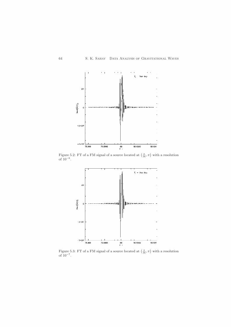
64 S. K. Sahay Data Analysis of Gravitational Waves
Figure 5.2: FT of a FM signal of a source located at`
π36
, π´
with a resolutionof 10−6.
Figure 5.3: FT of a FM signal of a source located at`
π36
, π´
with a resolutionof 10−7.

Chapter 5 Data Analysis — Part I 65
represents such a plot for
f0 = 80 Hz , h0 = h× = 1
α = π3, β0 = π
4, γ = 2π
5
θ = π36, φ = π , ψ = π
6
(5.43)
with the resolution 1/T0 =1.16×10⁻⁵ Hz. Figs. (5.2) and (5.3) representthe plot of the FT at resolution 10−6 Hz and 10−7 Hz. A careful look atthese plots reveals that the resolution of Fig. (5.1) does not representthe details of the dominant peaks around f0, whereas, Fig. (5.3) does notgive any new behaviour as compared to Fig. (5.2). Hence, we may saythat a resolution of about 10−6 Hz is required to understand the correctbehaviour of the FT for one day observation time data analysis. In thisreference we recall that the data analysis for the Fast Fourier Trans-form (FFT) limits the resolution to 1/T0. However, the detector outputmay provide us higher resolution. Thus the semi-analytical analysispresented here may provide more information as compared to FFT.
§5.4 Fourier transform of the complete response
The complete response R(t), in view of Eqs. (5.5), (5.16), (5.17), (5.30),and (5.31) may be written as
R(t) = R+(t) +R×(t) , (5.44)
R+(t) = h0+
[F1+ cos 2β + F2+ sin 2β + F3+ cosβ
+ F4+ sinβ + F5+
]cos
[Φ(t)
], (5.45)
R×(t) = h0×[F1× cos 2β + F2× sin 2β + F3× cosβ
+ F4× sinβ + F5×]sin
[Φ(t)
]. (5.46)
Here we have taken for simplicity the angles between the arms ofthe detector to be π
2i.e. Ω = π
4. Now the FT of the complete response
may be expressed asR(f) = R+(f) + R×(f) . (5.47)
To evaluate these we substitute β as given by (5.24). One obtains
R+(t) = h0+
[12
e−i2β0(F1+ + iF2+) e−i2wrot t +
+ ei2β0(F1+ − iF2+) ei2wrot t + e−iβ0(F3+ + iF4+) e−iwrot t
+ eiβ0(F3+ − iF4+) eiwrot t
+ F5+
]cos
[Φ(t)
](5.48)
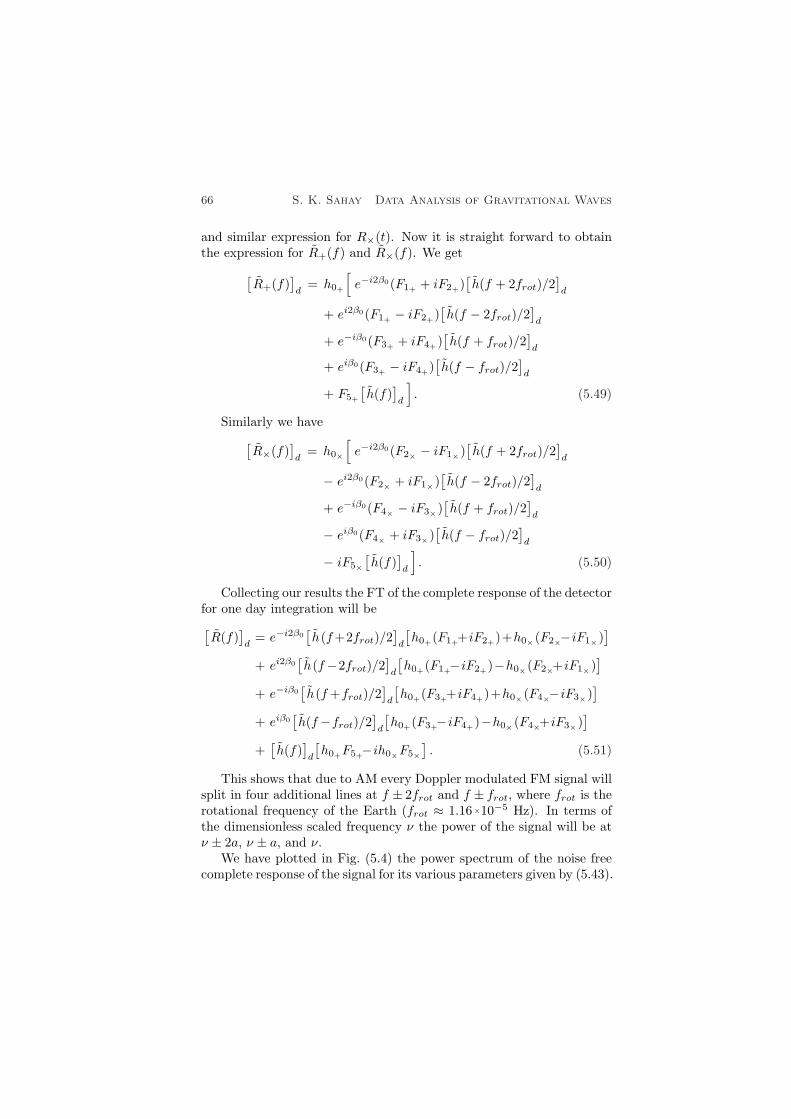
66 S. K. Sahay Data Analysis of Gravitational Waves
and similar expression for R×(t). Now it is straight forward to obtainthe expression for R+(f) and R×(f). We get
[R+(f)
]d
= h0+
[e−i2β0(F1+ + iF2+)
[h(f + 2frot)/2
]d
+ ei2β0(F1+ − iF2+)[h(f − 2frot)/2
]d
+ e−iβ0(F3+ + iF4+)[h(f + frot)/2
]d
+ eiβ0(F3+ − iF4+)[h(f − frot)/2
]d
+ F5+
[h(f)
]d
]. (5.49)
Similarly we have[R×(f)
]d
= h0×
[e−i2β0(F2× − iF1×)
[h(f + 2frot)/2
]d
− ei2β0(F2× + iF1×)[h(f − 2frot)/2
]d
+ e−iβ0(F4× − iF3×)[h(f + frot)/2
]d
− eiβ0(F4× + iF3×)[h(f − frot)/2
]d
− iF5×[h(f)
]d
]. (5.50)
Collecting our results the FT of the complete response of the detectorfor one day integration will be[R(f)
]d
= e−i2β0[h(f+2frot)/2
]d
[h0+(F1++iF2+)+h0×(F2×−iF1×)
]
+ ei2β0[h(f−2frot)/2
]d
[h0+(F1+−iF2+)−h0×(F2×+iF1×)
]
+ e−iβ0[h(f+frot)/2
]d
[h0+(F3++iF4+)+h0×(F4×−iF3×)
]
+ eiβ0[h(f−frot)/2
]d
[h0+(F3+−iF4+)−h0×(F4×+iF3×)
]
+[h(f)
]d
[h0+F5+−ih0×F5×
]. (5.51)
This shows that due to AM every Doppler modulated FM signal willsplit in four additional lines at f ± 2frot and f ± frot, where frot is therotational frequency of the Earth (frot ≈ 1.16×10⁻⁵ Hz). In terms ofthe dimensionless scaled frequency ν the power of the signal will be atν ± 2a, ν ± a, and ν.
We have plotted in Fig. (5.4) the power spectrum of the noise freecomplete response of the signal for its various parameters given by (5.43).
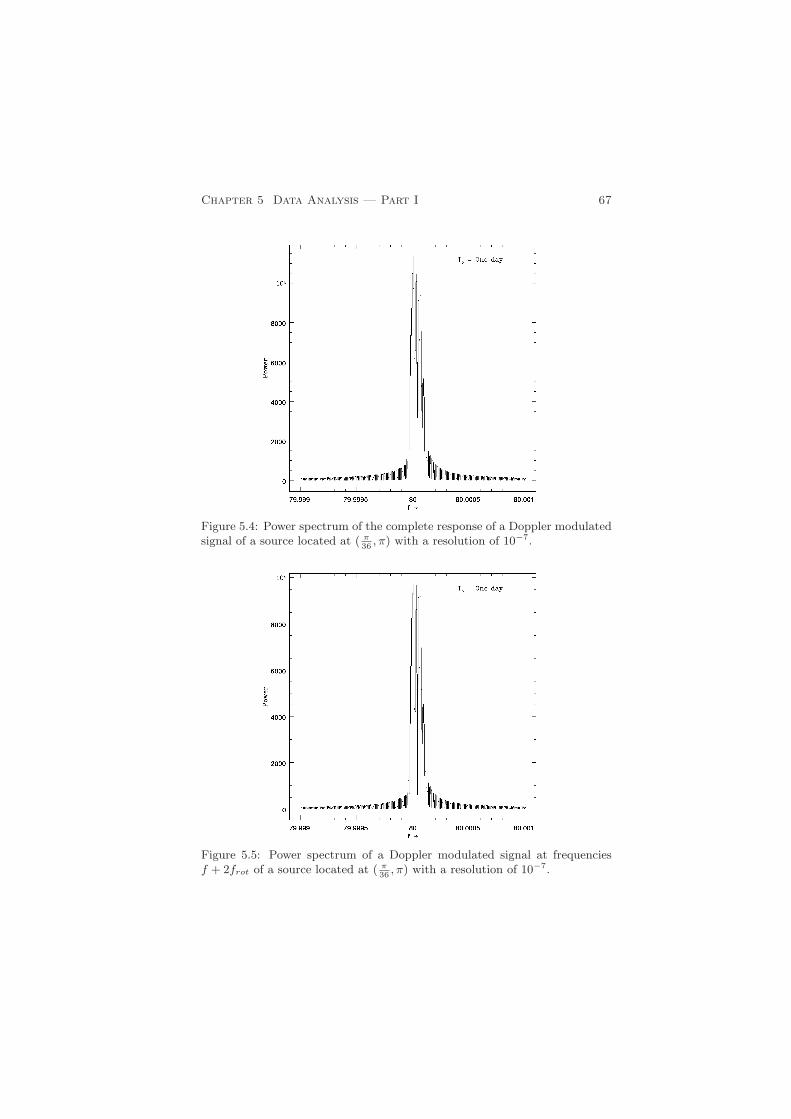
Chapter 5 Data Analysis — Part I 67
Figure 5.4: Power spectrum of the complete response of a Doppler modulatedsignal of a source located at ( π
36, π) with a resolution of 10−7.
Figure 5.5: Power spectrum of a Doppler modulated signal at frequenciesf + 2frot of a source located at ( π
36, π) with a resolution of 10−7.
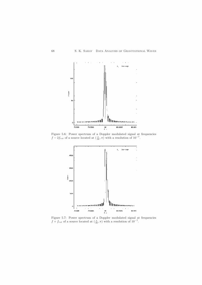
68 S. K. Sahay Data Analysis of Gravitational Waves
Figure 5.6: Power spectrum of a Doppler modulated signal at frequenciesf − 2frot of a source located at ( π
36, π) with a resolution of 10−7.
Figure 5.7: Power spectrum of a Doppler modulated signal at frequenciesf + frot of a source located at ( π
36, π) with a resolution of 10−7.
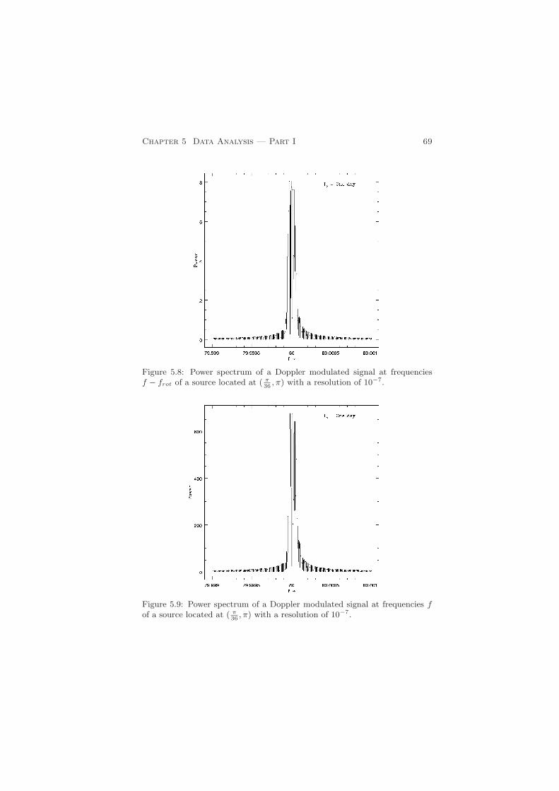
Chapter 5 Data Analysis — Part I 69
Figure 5.8: Power spectrum of a Doppler modulated signal at frequenciesf − frot of a source located at ( π
36, π) with a resolution of 10−7.
Figure 5.9: Power spectrum of a Doppler modulated signal at frequencies fof a source located at ( π
36, π) with a resolution of 10−7.
70 S. K. Sahay Data Analysis of Gravitational Waves
The contribution in the power spectrum of modulation at frequen-cies f +2frot, f − 2frot, f + frot, f − frot, and f are represented inFigs. (5.5), (5.6), (5.7), (5.8), and (5.9). It is observed that the most ofthe power will be at f +2frot, and least power will be in f − frot.
§5.5 Discussion
We have considered the effect of the Earth’s motion on the responseof the detector through FT analysis. It can easily be inferred fromEqs. (5.51) and (5.41, 5.42) that the splitting of the frequencies (i) arisesexplicitly in AM due to the rotational motion, and (ii) arises in FM dueto the rotational as well as the orbital motion of the Eearth. In view ofthe fact that the data output at the detector is available in discrete form,the analytical FT is not very convenient and one normally employs thepopular FFT. However, FFT has a resolution limited to 1/T0. Further,it is important to understand for how much time one can ignore thefrequency shift arising due to Doppler effect. In fact, Schutz (1991)has demonstrated that these effects due to the rotational motion areimportant after the time given by
Tmax =(
2cω2
rot f0Re
)1/2
' 70(
f01kHz
)−1/2
min . (5.52)
This means that for GW signal at the frequency 80 Hz one has totake into account these effects after data time '4 hours. The analyticalFT studied in this Chapter leads to following inferences:
(i) FFT for one day observation data will not provide such a sufficientresolution as to represent the correct picture of the frequency split-ting;
(ii) The adequate resolution required for one day observation is '10−6 Hz;
(iii) The frequency splitting due to FM for the frequency f0 = 80 Hzand source at (θ, φ) = ( π
36, π) is ' 2×10⁻⁴ Hz, while due to AM it
is ' 4.64×10⁻⁵ Hz;(iv) The drop in amplitude due to FM alone is about 56%;(v) The drop in amplitude due to AM alone is about 18%;(vi) The drop in amplitude for the complete response is about 74%;(vii) The maximum power due to AM is associated with f0 + 2frot.
It is remarked that the drop of the amplitude in complete responseis severe due to both AM and FM as the relevant frequency range lie inthe same region; see conclusion (iii) that above.
Chapter 5 Data Analysis — Part I 71
Finally, we would like to mention that we have presented the FTanalysis assuming the phase of the GW to be zero at the instant t = 0.However, one may relax this condition and may obtain the results easilyby taking into consideration the effects of change of the time origin.

Chapter 6
DATA ANALYSIS — PART II
§6.1 Introduction
In Chapter 5 we analyzed the Fourier analysis of one day observationdata set of the response of a laser interferometer. We have seen that theamplitude and frequency modulations result into a large number of sidebands about the signal frequency f0. Consequently the maximum powerlies in the frequency f + 2frot with the amplitude reduction by 74% towhat one would have expected due to the increased data interval. Hence,for GW detection it is desirable to obtain FT for larger data observationtime intervals. To begin with we present in the next §6.2 an analysisfor data set of one year observation time. The analysis turns out to besimple in view of the observation that there exists correspondences andidentifications to the analysis of Chapter 5 to make them identical. Inthis Chapter we generalize the results for an arbitrary observation time.To facilitate analogous modifications we have introduced correspondingquantities with tilde viz., C, and D in the place of C and D. As anapplication of the results we have obtained the FT for the spin downand N-component signal.
§6.2 Fourier transform for one year integration
§6.2.1 Frequency modulation
Let us rewrite the expression for phase of the GW signal referring toEqs. (5.27), (5.28), and (5.29), as follows
Φ(t) = 2πf0 t+ Z cos(worbt− φ
)+N cos
(wrot t− δ
)−R−Q . (6.1)
The FT for one year observation time Tobs is given as
[h(f)
]y
=∫ aT
0
cos[Φ(t)
]e−i2πft dt , (6.2)
a = a−1 = wrot/worb , T = one sidereal day , (6.3)
Tobs = a T ' 3.14×10⁷ sec . (6.4)
Chapter 6 Data Analysis — Part II 73
This may be split as usual into two terms as[h(f)
]y
= Iν− + Iν+ ; (6.5)
Iν− =1
2worb
∫ 2π
0
ei[ξν−+Z cos(ξ−φ)+N cos(aξ−δ)−R−Q] dξ , (6.6)
Iν+ =1
2worb
∫ 2π
0
e−i[ξν++Z cos(ξ−φ)+N cos(aξ−δ)−R−Q] dξ , (6.7)
ν± =f0 ± f
forb; ξ = ξorb = worbt . (6.8)
Hereafter, we neglect the contribution of Iν+ into[h(f)
]y
as it os-cillates rapidly and contributes very little, and we write ν in the placeof ν−. A careful comparison of Eq. (6.6) with (5.35) reveals that the in-tegrands of the equations are identical with the following identificationsand correspondences
δ ↔ φZ ↔ Na ↔ a
. (6.9)
Hence, we may employ the results obtained here by introducing ob-vious corresponding quantities, i.e. B, C, D in the place of B, C, D,leaving A unchanged. Thus
[h(f)
]y' ν
2worb
k=∞∑
k=−∞
m=∞∑m=−∞
eiA B [ C − iD ]; (6.10)
A =(k +m)π
2−R−Q ,
B =Jk(N )Jm(Z)ν2 − (ak +m)2
,
C = sin 2νπ cos (2akπ − kδ −mφ)
− ak +m
ν
cos 2νπ sin (2akπ − kδ −mφ) + sin (kδ +mφ)
,
D = cos 2νπ cos (2akπ − kδ −mφ)
+ka+m
νsin 2νπ sin (2akπ − kδ −mφ)− cos (kδ +mφ) .
Now the FT of these two polarization states can be written as
[h+(f)
]y
= h0+
[h(f)
]y' νh0+
2worb
k=∞∑
k=−∞
m=∞∑m=−∞
eiA B [ C − iD ], (6.11)
74 S. K. Sahay Data Analysis of Gravitational Waves
[h×(f)
]y
= −ih0×[h(f)
]y' νh0×
2worb
k=∞∑
k=−∞
m=∞∑m=−∞
eiA B [D−i C ]. (6.12)
The FT obtained contains the double series of Bessel functions ofthe order k and m ranging from −∞ to ∞. It is well known that Besselfunctions decrease rapidly as the order exceeds the argument. Hencethe possible range of k and m, over which the summation of the seriesis to be considered, depends on the arguments of Bessel functions i.e.Z and N . Referring to Eq. (5.28) it is found that
Zmax = 3133215(
f
1 KHz
)
Nmax = 134(
f
1 KHz
)
. (6.13)
The FT of a FM signal for
f0 = 50 Hz , h0 = h× = 1
α = π4, β0 = 0 , γ = π
θ = π18, φ = 0 , ψ = π
4
(6.14)
is shown in Fig. (6.1). A resolution of 1/T0 ≈ 3.17×10⁻⁸ Hz is attributedto the spectrum. We have convinced ourselves by plotting the FT athigher resolutions that the resolution of 1/T0 is sufficient to representrelevant peaks. We notice that the drop in amplitude is about 98%.This may be attributed to the presence of a very large number of sidebands.
§6.2.2 Complete response
The complete response of the detector may be obtained employingEqs. (6.11, 6.12, 5.45, 5.46) and one gets
[R+(f)
]y
= h0+
[e−i2β0(F1+ + iF2+)
[h(f + 2frot)/2
]y
+ ei2β0(F1+ − iF2+)[h(f − 2frot)/2
]y
+ e−iβ0(F3+ + iF4+)[h(f + frot)/2
]y
+ eiβ0(F3+ − iF4+)[h(f − frot)/2
]y
+ F5+
[h(f)
]y
], (6.15)

Chapter 6 Data Analysis — Part II 75
Figure 6.1: FT of a FM signal of a source located at ( π18
, 0) with a resolutionof 3.17× 10⁻⁸.
Figure 6.2: Power spectrum of the complete response of a modulated signalof a source located at ( π
18, 0) with a resolution of 3.17× 10⁻⁸.
76 S. K. Sahay Data Analysis of Gravitational Waves
[R×(f)
]y
= h0×
[e−i2β0(F2× − iF1×)
[h(f + 2frot)/2
]y
− ei2β0(F2× + iF1×)[h(f − 2frot)/2
]y
+ e−iβ0(F4× − iF3×)[h(f + frot)/2
]y
− eiβ0(F4× + iF3×)[h(f − frot)/2
]y
− iF5×[h(f)
]y
]. (6.16)
After rearranging these expressions we obtain[R(f)
]y
= e−i2β0[h(f+2frot)/2
]y
[h0+(F1++iF2+)+h0×(F2×−iF1×)
]
+ ei2β0[h(f−2frot)/2
]y
[h0+(F1+−iF2+)−h0×(F2×+iF1×)
]
+ e−iβ0[h(f+frot)/2
]y
[h0+(F3++iF4+)+h0×(F4×−iF3×)
]
+ eiβ0[h(f−frot)/2
]y
[h0+(F3+−iF4+)−h0×(F4×+iF3×)
]
+[h(f)
]y
[h0+F5+−ih0×F5×
]. (6.17)
Figure (6.2) shows the power spectrum of the complete response ofthe Doppler modulated signal. We have kept here all parameters thesame as in FM.
§6.3 Fourier transform for an arbitrary observation time
It is important to obtain the FT for an arbitrary observation time. Theresults obtained will be employed to outline how the spin down of apulsar due to the gravitational radiation back reaction or due to someother mechanism can be taken into account.
The FT for data of observation time T0 is given via
h(f) =∫ T0
0
cos[Φ(t)
]e−i2πft dt . (6.18)
As usual, this splits into two terms as
h(f) = Iν− + Iν+ ; (6.19)
Iν− =1
2wrot
∫ ξ0
0
ei[ξν−+Z cos(aξ−φ)+N cos(ξ−δ)−R−Q] dξ , (6.20)
Iν+ =1
2wrot
∫ ξ0
0
e−i[ξν++Z cos(aξ−φ)+N cos(ξ−δ)−R−Q] dξ , (6.21)

Chapter 6 Data Analysis — Part II 77
ν± =f0 ± f
frot; ξ0 = wrotT0 ; ξ = ξrot = wrot t . (6.22)
As Iν+ contributes very little into h(f), we drop Iν+ and write ν inthe place of ν−. Using the identity (5.38) we get
h(f) ' ei(−R−Q)
2wrot
∫ ξ0
0
eiνξ
[J0(Z) + 2
k=∞∑
k=1
Jk(Z)ik cos k (aξ − φ)]
×[J0(N ) + 2
m=∞∑m=1
Jm(N )im cosm(ξ − δ)]dξ . (6.23)
After performing the integration, we have
h(f) ' ν
2wrot
k=∞∑
k=−∞
m=∞∑m=−∞
eiAB [ C − iD ]; (6.24)
A =(k +m)π
2−R−Q , B =
Jk(Z)Jm(N )ν2 − (ak +m)2
,
C = sin ν ξ0 cos (akξ0 +mξ0 − kφ−mδ)
− ak +m
ν
cos ν ξ0 sin (akξ0 +mξ0 − kφ−mδ) + sin (kφ+mδ)
,
D = cos ν ξ0 cos (akξ0 +mξ0 − kφ−mδ)
+ka+m
νsin ν ξ0 sin (akξ0 +mξ0 − kφ−mδ)− cos (kφ+mδ) .
The FT of these two polarization states of the wave can be written
h+(f) = h0+ h(f) ' ν h0+
2wrot
k=∞∑
k=−∞
m=∞∑m=−∞
eiAB [ C − iD ], (6.25)
h×(f) = − ih0× h(f) ' ν h0×
2wrot
k=∞∑
k=−∞
m=∞∑m=−∞
eiAB [D − i C ]. (6.26)
Now it is simple to obtain the FT of complete response. One gets
R(f) = e−i2β0 h(f + 2frot)/2[h0+(F1++iF2+)+h0×(F2×−iF1×)
]
+ ei2β0 h(f−2frot)/2[h0+(F1+−iF2+)−h0×(F2×+iF1×)
]
+ e−iβ0 h(f+frot)/2[h0+(F3++iF4+)+h0×(F4×−iF3×)
]
+ eiβ0 h(f−frot)/2[h0+(F3+−iF4+)−h0×(F4×+iF3×)
]
+ h(f)[h0+F5+−ih0×F5×
]. (6.27)

78 S. K. Sahay Data Analysis of Gravitational Waves
Figure 6.3: FT of a FM signal of a source located at ( π9, π
4) with a resolution
of 9.67× 10⁻⁸.
The FT of FM signal for a data of 120 days and
f0 = 25 Hz , h0 = h× = 1
α = π6, β0 = π
3, γ = 2π
3
θ = π9, φ = π
4, ψ = π
4
(6.28)
are plotted in Figure (6.3) with a resolution of 12T0≈ 9.67×10⁻⁸ Hz. The
corresponding power spectra are plotted in Figure (6.4).
§6.4 Spin down
Pulsars loose the rotational energy by the processes like electro-magneticbreaking, particles emission, and GW emission. Thus, the rotationalfrequency is not completely stable, but varies over a time scale whichis of the order of the age of the pulsar. Typically, younger pulsars havelargest spin down rates. Current observations suggest that spin down isprimarily due to electro-magnetic breaking (Manchester, 1992; Kulkar-ni, 1992). Over the entire observing time T0 the frequency drift wouldbe small but it may be taken into account for better sensitivity. Toaccount this aspect we consider the evaluation of FT in a sequence of
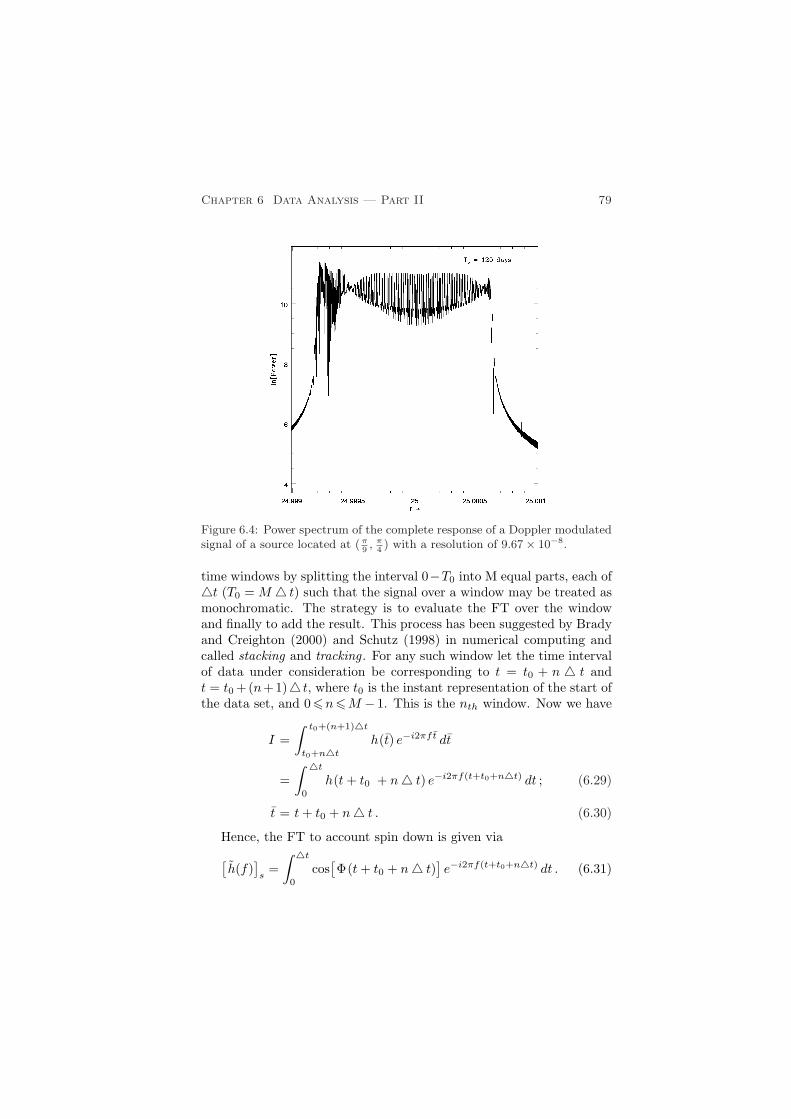
Chapter 6 Data Analysis — Part II 79
Figure 6.4: Power spectrum of the complete response of a Doppler modulatedsignal of a source located at (π
9, π
4) with a resolution of 9.67× 10⁻⁸.
time windows by splitting the interval 0−T0 into M equal parts, each of4t (T0 = M 4 t) such that the signal over a window may be treated asmonochromatic. The strategy is to evaluate the FT over the windowand finally to add the result. This process has been suggested by Bradyand Creighton (2000) and Schutz (1998) in numerical computing andcalled stacking and tracking . For any such window let the time intervalof data under consideration be corresponding to t = t0 + n 4 t andt = t0 +(n+1)4 t, where t0 is the instant representation of the start ofthe data set, and 0 6n6M − 1. This is the nth window. Now we have
I =∫ t0+(n+1)4t
t0+n4t
h(t) e−i2πft dt
=∫ 4t
0
h(t+ t0 + n4 t) e−i2πf(t+t0+n4t) dt ; (6.29)
t = t+ t0 + n4 t . (6.30)
Hence, the FT to account spin down is given via
[h(f)
]s
=∫ 4t
0
cos[Φ(t+ t0 + n4 t)
]e−i2πf(t+t0+n4t) dt . (6.31)

80 S. K. Sahay Data Analysis of Gravitational Waves
Taking the initial time of the data set
t0 = 0 , (6.32)
and following with the same way as in the previous §6.3, the FT isobtained as
[h(f)
]s' ei[2πn(f0−f)4t−R−Q]
2wrot
∫ 4t
0
eiνξ
×[J0(Z) + 2
k=∞∑
k=1
Jk(Z)ik cos k (aξ − λ)]
×[J0(N ) + 2
m=∞∑m=1
Jm(N )im cosm (ξ − ζ)]dξ . (6.33)
After integration we get
[h(f)
]s
=ν
2wrot
k=∞∑
k=−∞
m=∞∑m=−∞
eiAsB [Cs − iDs
], (6.34)
where
As =(k +m)π
2+ 2πn4 t(f0 − f)−R−Q
B =Jk(Z)Jm(N )ν2 − (ak +m)2
Cs = sin (ν τ) cos (akτ +mτ − kλ−mζ)
− ak +m
ν
cos (ν τ) sin (akτ +mτ − kλ−mζ)
+ sin (kλ+mζ)
Ds = cos (ν τ) cos (akτ +mτ − kλ−mζ)
+ak +m
νsin (ν τ) sin (akτ +mτ − kλ−mζ)
− cos (kλ+mζ)
λ = φ− anτ0 , ζ = δ − nτ0
τ = ξ0 = wrotT0 , τ0 = wrot 4 t
n = 0, 1, 2, 3, . . . ,M − 1
. (6.35)
Chapter 6 Data Analysis — Part II 81
The FT of the complete response would now be given via[R(f)
]s
= e−i2β0[h(f+2frot)/2
]s
[h0+(F1++iF2+)+h0×(F2×−iF1×)
]
+ ei2β0[h(f−2frot)/2
]s
[h0+(F1+−iF2+)−h0×(F2×+iF1×)
]
+ e−iβ0[h(f+frot)/2
]s
[h0+(F3++iF4+)+h0×(F4×−iF3×)
]
+ eiβ0[h(f−frot)/2
]s
[h0+(F3+−iF4+)−h0×(F4×+iF3×)
]
+[h(f)
]s
[h0+F5+−ih0×F5×
]. (6.36)
§6.5 N-component signal
The FT in Eqs. (6.24) and (6.27) are for a pulsar which emits GW signalat a single frequency f0. But there are known physical mechanismswhich generate GW signals consisting of many components. An axiallysymmetric pulsar undergoing free precession, emits a quadrupole GWat two frequencies, one equal to the sum of the spin frequency and theprecession frequency, and the other twice of it (Zimmermann, 1979,1980). The quadrupole GW from a triaxial ellipsoid rotating about oneof its axes consists of one component only (Thorne, 1987). In this casethe signal has a frequency about twice the spin frequency of the star.In general, if a star is non-axisymmetric and precessing, the GW signalconsists of more than two components. For the case of triaxial ellipsoidand small wobble angle there is a third component with a frequencytwice of the spin frequency of the star (Zimmermann, 1979, 1980). Also,the mechanisms e.g. the r-mode instability of spinning neutron stars(Anderson, 1998; Lindblom et al., 1998; Owen et al., 1998) and thetemperature asymmetry in the interior of a neutron star with the miss-aligned spin axis (Bildsten, 1998) have been discussed in the literature.
In view of the above discussion CGW signal may consists of frequen-cies which are multiple of some basic frequencies. An analysis of theGW data of N-component of signal has been made recently by Jara-nowski and Krolak (2000). In this §6.5 we present Fourier analysis ofan N-component CGW signal. We model the N-component signal as
h(t) =N∑
l=1
hl(t) ; (6.37)
hl+(t) = h0l+ cos[Φl(t)
], (6.38)
hl×(t) = h0l× sin[Φl(t)
], l = 1, 2, . . . , N ; (6.39)

82 S. K. Sahay Data Analysis of Gravitational Waves
Φl(t)= 2πfl
[t+Zl cos (aξrot−φ) +Nl cos(ξrot−δl)−Rl−Ql
], (6.40)
where fl represent the component frequency of the signal.Now let us write
hl(t) = cos[Φl(t)
]. (6.41)
It is trivial matter to obtain hl(f), Rl(f), and to get
hN (f) =∑
l
hl(f) , (6.42)
RN (f) =∑
l
Rl(f) . (6.43)
§6.6 Discussion and summary
The analysis and results obtained in the previous Chapter 5 regardingFT of the response of a laser interferometer have been generalized inthe present Chapter. In this context following points must be noted:
1. For longer observation time, say, 120 days the resolution providedby FFT (equal to 1/T0) is sufficient to represent the structure ofside bands;
2. Although in every case discussed, it turned out that the maximumpower lies in the frequency f + 2frot. However, this is not estab-lished conclusively whether this result is generic. In any case, forany given detector location, we can know in advance if a similartype of behaviour is obtained;
3. The computer time required in computing analytical FT dependson the orientation of the source, and is independent from the timeinterval of the observation data set. In contrast to this factor,the computation cost increases for FFT with the increase of thedata set;
4. Throughout our analysis in Chapters 5 and 6 we have employedfollowing conditions:
(i) The phase of the wave is zero at t = 0;(ii) The observation time of the data set is in the range from
t = 0 to t = T0;
5. As remarked in Chapter 5 the requirement 4(i) may be achievedby translation of time-origin. Now let us see how the condition4(ii) can be relaxed. Let the data set is taken for
t = ti to t = ti + T0 . (6.44)
Chapter 6 Data Analysis — Part II 83
Eqs. (6.29, 6.30, 6.31, 6.32) reveal that the results obtained therecorrespond to data set
t = n4 t to t = (n+ 1)4 t . (6.45)
To obtain the sought generalization we set
ti = n4 t and T0 = 4t , (6.46)
and may use the results of §6.3 by noting that for the present casewe have
λ = φ− nworb 4 t =⇒ λ = φ− worb ti , (6.47)
ζ = δ − nwrot 4 t =⇒ ζ = δ − wrot ti . (6.48)
Chapter 7
TEMPLATES FOR AN ALL SKY SEARCH
§7.1 Introduction
Gravitational wave laser interferometer antennae are essentially omni-directional with their response better than 50% of the average over 75%of the whole sky. Hence the data analysis systems will have to carryout all sky searches for the sources. We know that the amplitude of anintense GW believed bathing the Earth is very small, as compared tothe sensitivity of GW detectors and is further masked by the dominantnoise. In these circumstances, CGW sources are of prime importancebecause for such sources we can achieve enhanced SNR by investigat-ing longer observation data set. However, a long observation time in-troduces modulation effects, arising due to the relative motion of thedetector with respect to the source. As a consequence, there results adistribution of power in a forest of sidebands to such an extent thatthere is a reduction to the tune of 90% of the expected power due toAM. The problem of an all sky search gains another dimension in viewof the fact that there are reasons to believe the presence of intense GWsources whose locations and even frequencies are unknown. Amongstsuch sources pulsars occupy an important position. Similar to all skysearch one will also have to do all frequency search. All sky and allfrequency search is the holy grail of gravitation pulsar astronomy.
Search of CGW without a priori knowledge appears to be computa-tionally quite demanding even by the computers expected to be availablein the near future. For example, in the case of a bandwidth 103 Hz, anobservation time 107 sec, and a star’s minimum decay time of 100 yearsone would require 1014 TFLOPS computer (Frasca, 2000). Very fastcomputer and large memories with an ample amount of the disk spaceseems inevitable. However, the choice of optimal data processing andclever programming is also an integral part of the solution to this prob-lem. Amongst these the pre-correction of the time series due to Dopplermodulation before the data are processed may be a method, which willreduce computational requirements. In reference to this, Schutz (1991)has introduced the concept of patches in the sky defined as the region ofspace for which similar Doppler corrections would be required. He has
Chapter 7 Templates for an All Sky Search 85
also demonstrated that the number of the patches required for a 107 secobservation data set and one KHz signal would be about 1.3×10¹³, if onetakes into account the Earth’s rotation. However, the size of such apatch would also depend on the data analysis technique being employed.
Matched Filtering is the most suitable technique for detection of sig-nals from sources viz., pulsars whose wave form is known. The waveforms are used to construct a bank of templates, which represent theexpected signal wave form with all possible ranges of its parameters.The time of arrival, the source location, the frequency of the signal, theellipticity of the source and its spin down represent important param-eters of a GW emitted by a pulsar. For detection of GW we set upa criterion to judge if the cross correlation of the templates with thecorresponding data set exceeds the preassigned threshold. We wouldperform the data analysis employing the criterion of the FF.
§7.2 Matched filter analysis: templates
The bank of templates will be matched to only a discrete set of signalsfrom amongst the continuum of possible signals. Consequently, it isnatural that all the signals will not get detected with equal probabil-ity. However, it is possible to choose judiciously the set of templates sothat all signals of a given amplitude are detected with a given minimumdetection probability. The standard measure for deciding what class ofwave form is good enough is the FF (Apostolatos, 1995). It quantita-tively describes the closeness of the true signals to the template manifoldin terms of the reduction of SNR due to a cross correlation between asignal outside the manifold and all the templates lying inside the man-ifold. If the FF of a template family is unity, the signal lies in themanifold. If the FF is less than unity, the signal lies outside manifold.
Even if the signal discrete templates lies within the template man-ifold it would be unlikely that any of the actual templates used wouldcorrespond to the signal. The parameters describing the search tem-plate (the source location, the ellipticity, etc.) can vary continuouslythroughout a finite range of values. The set of templates characterizedby the continuously varying parameters is of course infinite. However, inpractice the interferometer output must be cross correlated with a finitesubset of the templates whose parameter values vary in discrete stepsfrom one template to the next one. This subset (“the discrete templatefamily”) is zero on the manifold of the full set of possible templates(“the continuous template family”), so the template which most closelymatch a signal will generally lie between the signal and the nearest of
86 S. K. Sahay Data Analysis of Gravitational Waves
the discrete template family. The mismatch between the signal and thenearest of the discrete templates will cause some reduction in SNR. Thiswould mean that the members of the discrete template family must bechosen so as to render acceptable loss of SNR.
The study of templates has been made by many researchers in timedomain.∗ However, the analysis in frequency domain has the advantageof incorporating interferometer’s spectral noise density. In order to de-termine the number of templates required to perform matched filteringanalysis let us rewrite the formula expressing FF , see Eq. (4.12), as
FF (θ, φ) = maxθ,φ
〈h(f)|hT (f ; θT , φT )〉√〈hT (f ; θT , φT )|hT (f ; θT , φT )〉〈h(f)|h(f)〉 , (7.1)
where h(f) and hT (f ; θT , φT ) are the FTs of the signal wave form andthe templates, respectively. The template parameters θT , φT are chosendiffering from the actual orientation of the source in discrete steps.
We have seen in the previous Chapters that the AM of CGW dataoutput results into re-distribution of power at four additional frequenciesf ± 2frot, f ± frot according to the FM. Hence it is sufficient for theanalysis of FF to consider only the frequency modulated FT. The resultsobtained in Chapter 6 regarding the FT of the frequency modulated dataoutput, see Eq. (6.24), may be arranged using the symmetry propertyof the Bessel functions, and one may write
h(f) ' ν
wrot
[J0(Z)J0(N )
2ν2
[sin (R+Q)− sin (R+Q− ν ξ0)
+
+ icos (R+Q)− cos (R+Q− ν ξ0)
]
+ J0(Z)m=∞∑m=1
Jm(N )ν2 −m2
[(YU − XV)− i(XU + YV)
]
+k=∞∑
k=1
m=∞∑m=−∞
eiAB [ C − iD ]], (7.2)
X = sin(R+Q−m π
2
)
Y = cos(R+Q−m π
2
)
U = sin ν ξ0 cosm(ξ0−δ)−m
νcos ν ξ0 sinm(ξ0−δ)− sinmδ
V = cos ν ξ0 cosm(ξ0−δ)+m
νsin ν ξ0 sinm(ξ0−δ)− cosmδ
. (7.3)
∗Schutz (1991), Brady et al. (1998), Brady and Creighton (2000), Jaranowski etal. (1998), Jaranowski and Krolak (2000).

Chapter 7 Templates for an All Sky Search 87
Figure 7.1: Variation of FF with θT .
Now it is straight forward to compute FF . To understand the proce-dure let us assume that there is a source at the location (θ, φ)= (25, 30)emitting a frequency f0 =0.5 Hz. We wish to analyze the data set forT0 = one sidereal day. We first fix the template parameter φ for thewhole set given by φT =φ=30 and vary θT in discrete steps over itsentire range i.e. 0 to 180. The results obtained are plotted graphicallyin Fig. (7.1). It is remarked that, in order to compute the inner prod-uct defined via Eq. (4.9), one would require to integrate the expressionover the band width of the Doppler modulated signal. This may bedetermined either analytically by computing the maximum value of theDoppler shift in accordance with Eq. (5.25) or may be taken as the rep-resented by the frequency spectrum of the FT. In the present case wehave taken the band width equal to 0.002 Hz. In a similar manner onemay fix the θ-parameter of the template set and obtain the variation ofFF with the template parameter φT . Figures (7.2) and (7.3) representrespectively the behaviour for f0 =25 Hz, θ= θT = 1, T0 = one siderealday for source orientation φ= 35 and 220.
The following points in reference to these plots may be noted:(i) The FF is unity for θT = 25, 155, see Fig (7.1, for φT = 35,
145, see Fig (7.2), and for φT = 220, 320, see Fig (7.3);
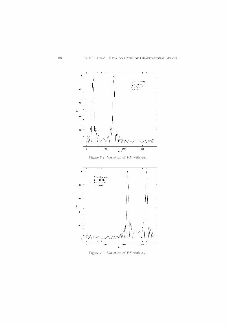
88 S. K. Sahay Data Analysis of Gravitational Waves
Figure 7.2: Variation of FF with φT .
Figure 7.3: Variation of FF with φT .

Chapter 7 Templates for an All Sky Search 89
(ii) It is observed that FF decreases exponentially with template vari-ables θT and φT . The specific relations are found numerically
FF = e−0.00788(θT−θ)2 , (7.4)
FF = e−0.01778(φT−φ)2 ; (7.5)
(iii) The oscillatory behaviours do not represent any real situation asit arises because of the improper choice of numerical integrationtechnique. However, we are content with the technique we haveemployed as the region of such artificial facets falls into the regionof FF < 0.25.
Finally, we end this §7.2 by noting but the symmetry property of thetemplate parameters. A closer look of the graphs and the remark (i) thatabove reveal the following symmetry property. The FF is symmetricalunder the following transformations
θT → π − θT , 0 6 θT 6 π ; (7.6)
φT → π − φT , 0 6 φT 6 π ; (7.7)
φT → 3π − φT , π 6 φT 6 2π . (7.8)
It should be noted that these symmetry properties are based onour results obtained for one sidereal day observation time. The genericnature of the symmetries may be established only after studying thevariation of FF with T0.
§7.3 The number of templates
It is important to study the problem of the number of templates for allsky search in the light of FF . The results of §7.2 reveal that the gridspacing 4θ in the θ-parameter of templates may be expressed symbol-ically as a function of FF , f0, and T0 i.e.
4θ = F(FF, f0, θ, φ, T0) . (7.9)Similarly, we have
4φ = G (FF, f0, θ, φ, T0) . (7.10)
In view of this, Equations (9.13) and (9.20) may be equivalentlyexpressed as
F(FF, 0.5, 25, 30, T ) =[−(0.00788)−1 ln(FF )
]1/2, (7.11)
G (FF, 25, 1, 35, T ) =[−(0.01788)−1 ln(FF )
]1/2. (7.12)
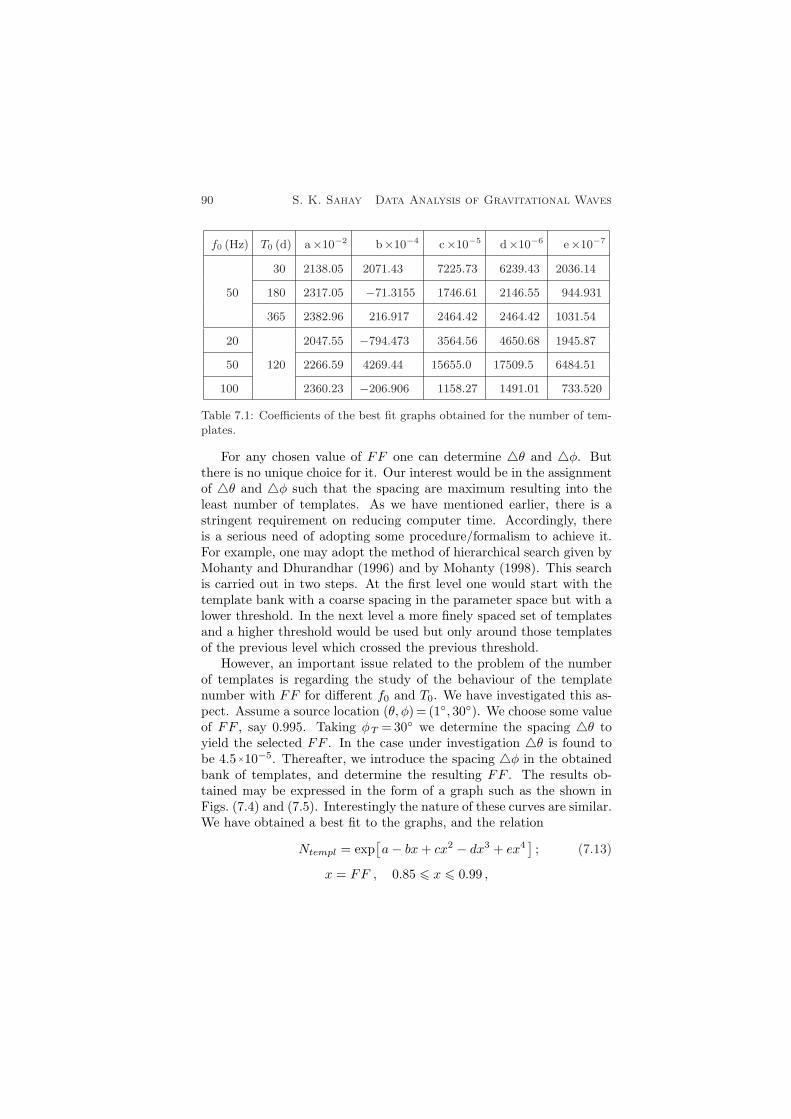
90 S. K. Sahay Data Analysis of Gravitational Waves
f0 (Hz) T0 (d) a×10−2 b×10−4 c×10−5 d×10−6 e×10−7
30 2138.05 2071.43 7225.73 6239.43 2036.14
50 180 2317.05 −71.3155 1746.61 2146.55 944.931
365 2382.96 216.917 2464.42 2464.42 1031.54
20 2047.55 −794.473 3564.56 4650.68 1945.87
50 120 2266.59 4269.44 15655.0 17509.5 6484.51
100 2360.23 −206.906 1158.27 1491.01 733.520
Table 7.1: Coefficients of the best fit graphs obtained for the number of tem-plates.
For any chosen value of FF one can determine 4θ and 4φ. Butthere is no unique choice for it. Our interest would be in the assignmentof 4θ and 4φ such that the spacing are maximum resulting into theleast number of templates. As we have mentioned earlier, there is astringent requirement on reducing computer time. Accordingly, thereis a serious need of adopting some procedure/formalism to achieve it.For example, one may adopt the method of hierarchical search given byMohanty and Dhurandhar (1996) and by Mohanty (1998). This searchis carried out in two steps. At the first level one would start with thetemplate bank with a coarse spacing in the parameter space but with alower threshold. In the next level a more finely spaced set of templatesand a higher threshold would be used but only around those templatesof the previous level which crossed the previous threshold.
However, an important issue related to the problem of the numberof templates is regarding the study of the behaviour of the templatenumber with FF for different f0 and T0. We have investigated this as-pect. Assume a source location (θ, φ)= (1, 30). We choose some valueof FF , say 0.995. Taking φT =30 we determine the spacing 4θ toyield the selected FF . In the case under investigation 4θ is found tobe 4.5×10⁻⁵. Thereafter, we introduce the spacing 4φ in the obtainedbank of templates, and determine the resulting FF . The results ob-tained may be expressed in the form of a graph such as the shown inFigs. (7.4) and (7.5). Interestingly the nature of these curves are similar.We have obtained a best fit to the graphs, and the relation
Ntempl = exp[a− bx+ cx2 − dx3 + ex4
]; (7.13)
x = FF , 0.85 6 x 6 0.99 ,
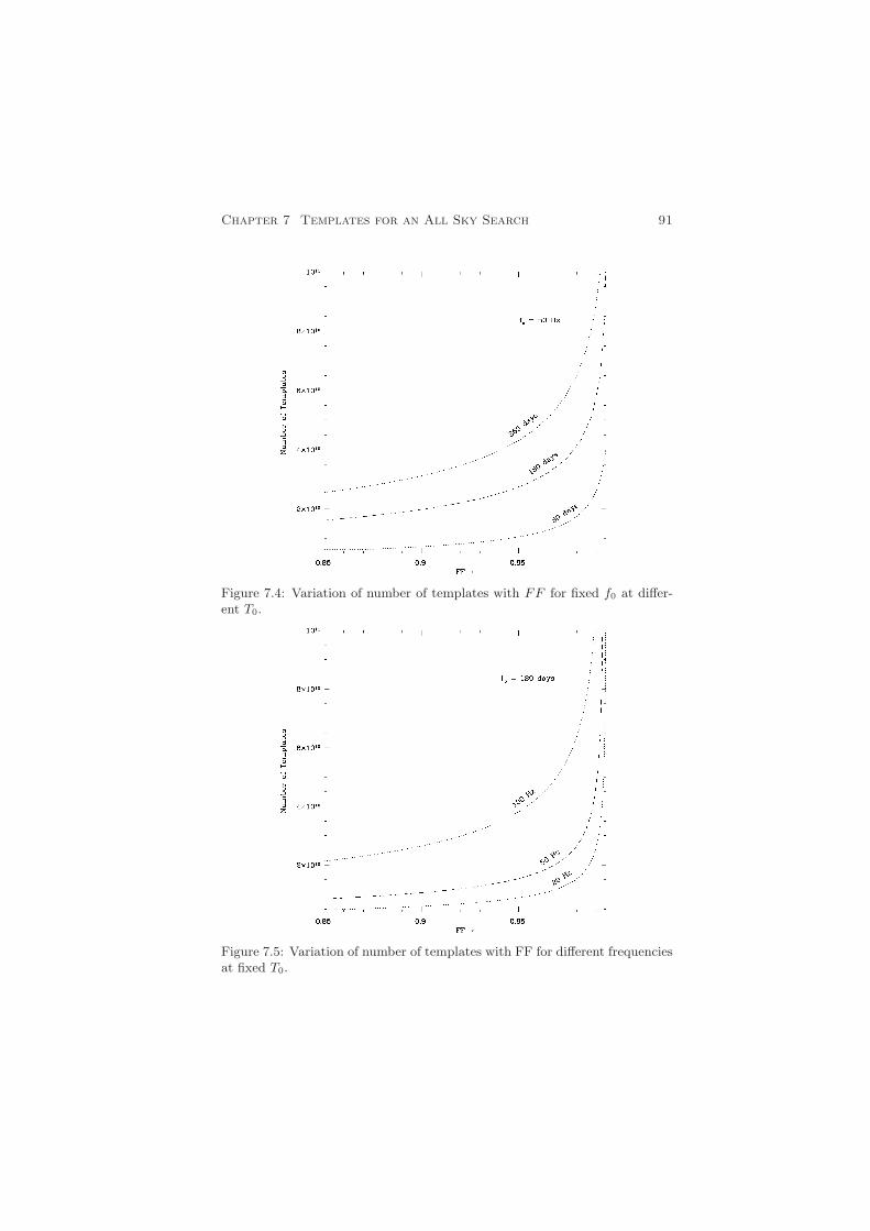
Chapter 7 Templates for an All Sky Search 91
Figure 7.4: Variation of number of templates with FF for fixed f0 at differ-ent T0.
Figure 7.5: Variation of number of templates with FF for different frequenciesat fixed T0.
92 S. K. Sahay Data Analysis of Gravitational Waves
where a, b, c, d and e are constants. The numerical values of theseconstants are given in Table (7.1).
Note from the graphs, for sake of comparison, that the numbersof templates required for FF equal to 0.97 are respectively 1.44×1010,3.5×1010, 5.5×10¹⁰ for the observation data set of 30, 120 365 days andf0 =50 Hz. Similarly the number of templates required to analyze theobservation data set of 120 days of GW frequencies 20, 50 and 100 Hzare respectively 1.22×10¹⁰, 2.16×10¹⁰, and 5×10¹⁰. It is observed thathigher FF requires exponentially increasing the number of templates.
§7.4 Discussion
In view of the complexity of the FT which contains exponential as well asBessel functions, one has to be careful in computing FF . We have founduseful to employ the Romberg integration using Pade approximation.We have used (i) QROMO of numerical recipes instead of QROMB asthe former takes care of singularities, and (ii) RATINT routine for Padeapproximation. The Bessel functions are computed using the routineBESSJ0(X), BESSJ1(X) and BESSJ(N,X) of numerical recipes (Presset al., 1986). The BESSJ0(X) and BESSJ1(X) compute the Bessel func-tion of the first kind of zeroth and first order respectively for any valueof X, while BESSJ(N, X) computes the Bessel function of first kind ofarbitrary integral order N for any value of X.
We have noticed marked symmetries in all sky search in both θ andφ space for one day observation time. It has been found that any FFcorresponds to two values each in θT and φT . Accordingly, computationburden will be reduced by a factor of four. However, it is not clearwhether the symmetry property can be established analytically as well.The source location, because of the symmetry, is uncertain. Some otheranalysis is to be adopted for getting the exact location.
We have computed the number of templates required for all skysearch for matched filtering assuming the noise power spectral densitySn(f) to be flat. However, for realistic situation, the effect of the noisehave to be taken into consideration.
The optimum template parametrization and placement, and the re-lated computational burden were discussed by Sathyaprakash and Dhu-randhar (1991), Dhurandhar and Sathyaprakash (1994), Owen (1996),Apostolatos (1995, 1996), Mohanty and Dhurandhar (1996), Mohanty(1998), Owen and Sathayaprakash (1999). The possible efficient inter-polated representation of the correlators is a problem of interest.
Chapter 8
MATCHING OF THE SIGNALS
§8.1 Introduction
The strength of CGW is largely dependent on the degree of the long-living asymmetry in the source. There are several mechanism for pro-ducing such an asymmetry (Pandharipande et al., 1976; Bonazzola andGourgoulhon, 1996; Zimmermann and Szedenits, 1979; Zimmermann,1980). The estimates of the asymmetry in neutron stars shows that theamplitude of CGW may be 6 10−25. Hence, long integration will berequired to get the signature of the signal. But this in turn inducesseveral other problems viz. Doppler modulation and non-stationarity ofthe noise in the detector.
Consequently data analysis becomes more, and more harder. How-ever, Doppler modulation will provide an information about the positionof the source in the sky.
The basic method to analyze the detector output to get the signatureof GW signals relies on how efficiently one can process Fourier analyisof the data. In Chapter 5 and 6 we shown that amplitude modulationwill only redistribute the power of the FM signal in five frequency bandsf±2frot, f , f±frot. Hence it is sufficient to consider only the FM signalfor the analysis of the matching of the signals from different locationsin the sky.
In the previous Chapter 7 the matching of the signals from locationsin the sky that differ in their co-latitude and longitude by π radians hasbeen made for 1-d data set and observed symmetries in the sky locationsunder the following transformations
θT → π − θT , 0 6 θT 6 π ; (8.1)
φT → π − φT , 0 6 φT 6 π ; (8.2)
φT → 3π − φT , π 6 φT 6 2π . (8.3)
However, it will be important to understand the generic nature ofthe matching of signals under the above transformations, and also checkit in practice.
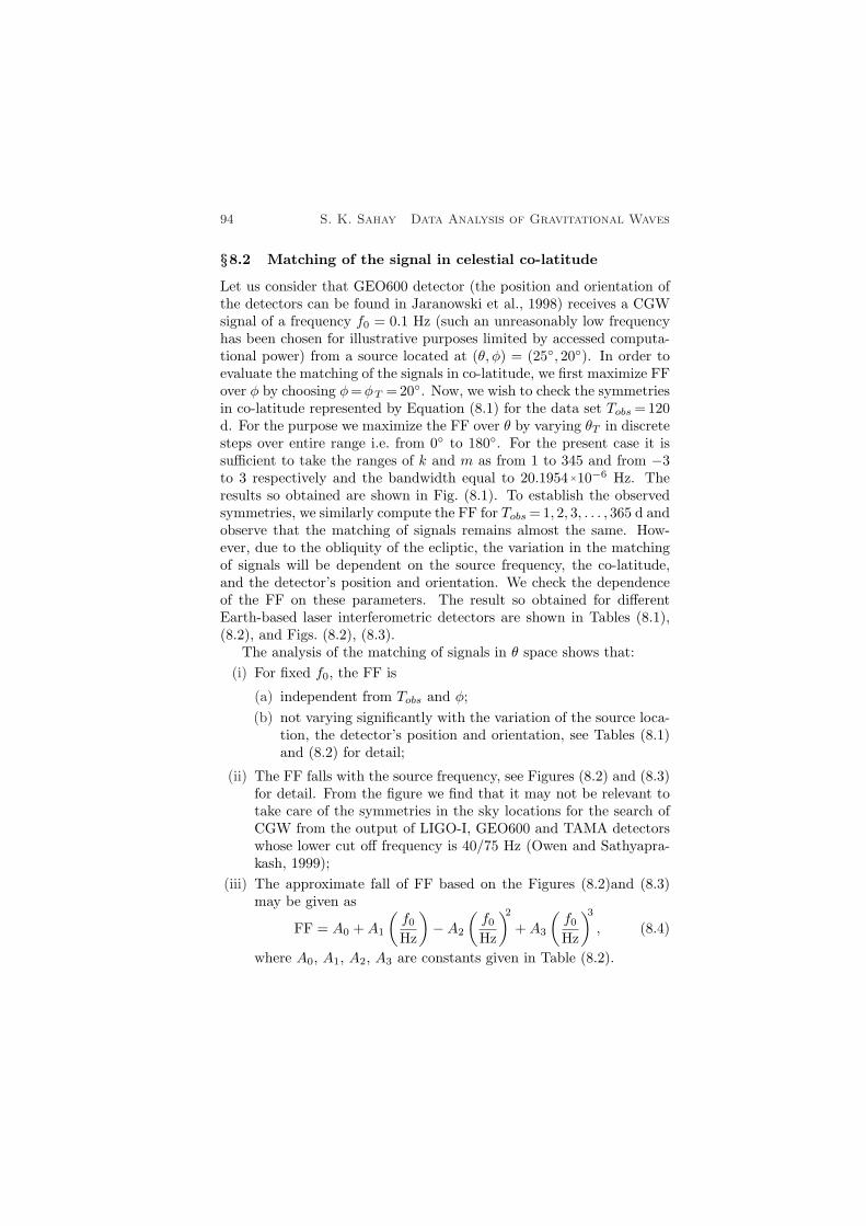
94 S. K. Sahay Data Analysis of Gravitational Waves
§8.2 Matching of the signal in celestial co-latitude
Let us consider that GEO600 detector (the position and orientation ofthe detectors can be found in Jaranowski et al., 1998) receives a CGWsignal of a frequency f0 = 0.1 Hz (such an unreasonably low frequencyhas been chosen for illustrative purposes limited by accessed computa-tional power) from a source located at (θ, φ) = (25, 20). In order toevaluate the matching of the signals in co-latitude, we first maximize FFover φ by choosing φ=φT =20. Now, we wish to check the symmetriesin co-latitude represented by Equation (8.1) for the data set Tobs =120d. For the purpose we maximize the FF over θ by varying θT in discretesteps over entire range i.e. from 0 to 180. For the present case it issufficient to take the ranges of k and m as from 1 to 345 and from −3to 3 respectively and the bandwidth equal to 20.1954×10⁻⁶ Hz. Theresults so obtained are shown in Fig. (8.1). To establish the observedsymmetries, we similarly compute the FF for Tobs = 1, 2, 3, . . . , 365 d andobserve that the matching of signals remains almost the same. How-ever, due to the obliquity of the ecliptic, the variation in the matchingof signals will be dependent on the source frequency, the co-latitude,and the detector’s position and orientation. We check the dependenceof the FF on these parameters. The result so obtained for differentEarth-based laser interferometric detectors are shown in Tables (8.1),(8.2), and Figs. (8.2), (8.3).
The analysis of the matching of signals in θ space shows that:(i) For fixed f0, the FF is
(a) independent from Tobs and φ;(b) not varying significantly with the variation of the source loca-
tion, the detector’s position and orientation, see Tables (8.1)and (8.2) for detail;
(ii) The FF falls with the source frequency, see Figures (8.2) and (8.3)for detail. From the figure we find that it may not be relevant totake care of the symmetries in the sky locations for the search ofCGW from the output of LIGO-I, GEO600 and TAMA detectorswhose lower cut off frequency is 40/75 Hz (Owen and Sathyapra-kash, 1999);
(iii) The approximate fall of FF based on the Figures (8.2)and (8.3)may be given as
FF = A0 +A1
(f0Hz
)−A2
(f0Hz
)2
+A3
(f0Hz
)3
, (8.4)
where A0, A1, A2, A3 are constants given in Table (8.2).
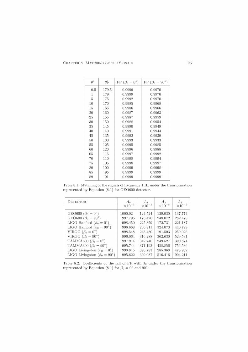
Chapter 8 Matching of the Signals 95
θ θT FF (β0 = 0) FF (β0 = 90)
0.5 179.5 0.9999 0.99701 179 0.9999 0.99705 175 0.9992 0.9970
10 170 0.9985 0.996815 165 0.9986 0.996620 160 0.9987 0.996325 155 0.9987 0.995930 150 0.9988 0.995435 145 0.9990 0.994940 140 0.9991 0.994445 135 0.9992 0.993950 130 0.9993 0.993355 125 0.9995 0.998560 120 0.9996 0.998865 115 0.9997 0.999270 110 0.9998 0.999475 105 0.9998 0.999780 100 0.9999 0.999885 95 0.9999 0.999989 91 0.9999 0.9999
Table 8.1: Matching of the signals of frequency 1 Hz under the transformationrepresented by Equation (8.1) for GEO600 detector.
Detector A0 A1 A2 A3
×10−3 ×10−5 ×10−5 ×10⁻⁷
GEO600 (β0 = 0) 1000.02 124.524 129.030 137.774GEO600 (β0 = 90) 997.796 175.426 248.072 282.478LIGO Hanford (β0 = 0) 998.450 225.359 172.731 221.187LIGO Hanford (β0 = 90) 996.668 266.811 324.073 440.729VIRGO (β0 = 0) 998.548 243.480 191.503 259.026VIRGO (β0 = 90) 996.064 316.288 362.630 529.531TAMMA300 (β0 = 0) 997.914 342.746 249.527 390.874TAMMA300 (β0 = 90) 995.744 371.193 458.856 756.536LIGO Livingston (β0 = 0) 998.815 396.783 285.368 478.932LIGO Livingston (β0 = 90) 995.622 399.087 516.416 904.211
Table 8.2: Coefficients of the fall of FF with f0 under the transformationrepresented by Equation (8.1) for β0 = 0 and 90.
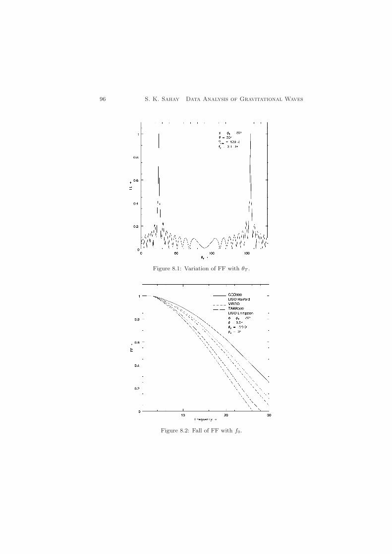
96 S. K. Sahay Data Analysis of Gravitational Waves
Figure 8.1: Variation of FF with θT .
Figure 8.2: Fall of FF with f0.
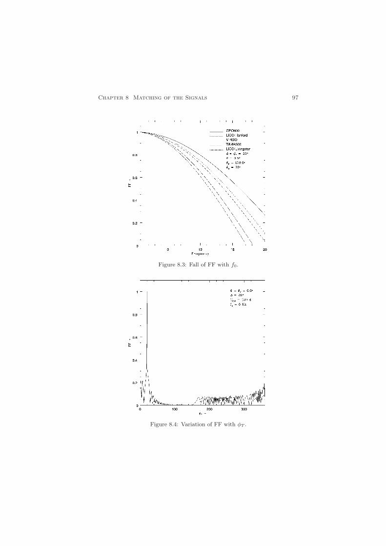
Chapter 8 Matching of the Signals 97
Figure 8.3: Fall of FF with f0.
Figure 8.4: Variation of FF with φT .
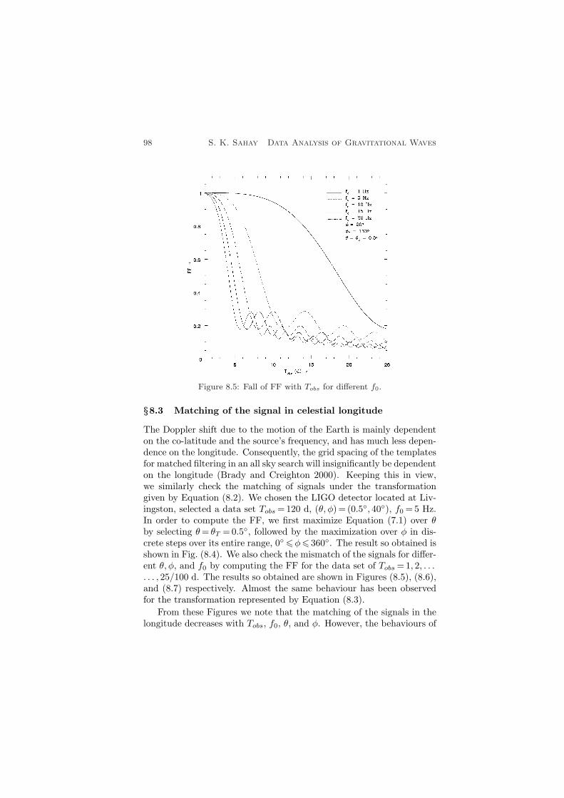
98 S. K. Sahay Data Analysis of Gravitational Waves
Figure 8.5: Fall of FF with Tobs for different f0.
§8.3 Matching of the signal in celestial longitude
The Doppler shift due to the motion of the Earth is mainly dependenton the co-latitude and the source’s frequency, and has much less depen-dence on the longitude. Consequently, the grid spacing of the templatesfor matched filtering in an all sky search will insignificantly be dependenton the longitude (Brady and Creighton 2000). Keeping this in view,we similarly check the matching of signals under the transformationgiven by Equation (8.2). We chosen the LIGO detector located at Liv-ingston, selected a data set Tobs =120 d, (θ, φ)= (0.5, 40), f0 =5 Hz.In order to compute the FF, we first maximize Equation (7.1) over θby selecting θ= θT =0.5, followed by the maximization over φ in dis-crete steps over its entire range, 06φ6 360. The result so obtained isshown in Fig. (8.4). We also check the mismatch of the signals for differ-ent θ, φ, and f0 by computing the FF for the data set of Tobs =1, 2, . . .. . . , 25/100 d. The results so obtained are shown in Figures (8.5), (8.6),and (8.7) respectively. Almost the same behaviour has been observedfor the transformation represented by Equation (8.3).
From these Figures we note that the matching of the signals in thelongitude decreases with Tobs, f0, θ, and φ. However, the behaviours of
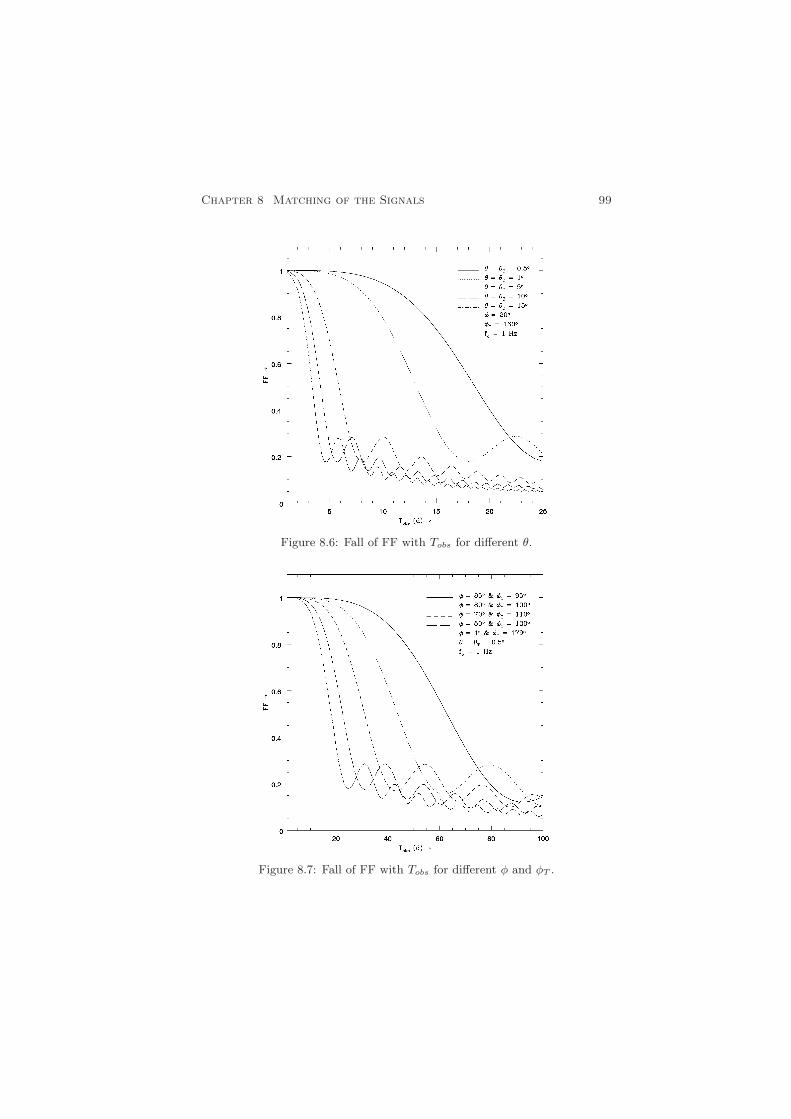
Chapter 8 Matching of the Signals 99
Figure 8.6: Fall of FF with Tobs for different θ.
Figure 8.7: Fall of FF with Tobs for different φ and φT .

100 S. K. Sahay Data Analysis of Gravitational Waves
f 0(H
z)θ
θ T
φ
φ T
B0×1
0−
3B
1×1
0−
5B
2×1
0−
5B
3×1
0−
6B
4×1
0−
7
20
1032.3
913167.8
14036.2
56606.5
55088.4
15
1030.8
511101.8
10398.0
36450.9
30710.3
10
0.5
0.5
1028.7
98750.1
86813.7
419603.4
13481.1
51025.7
35842.3
03302.2
16795.1
93310.2
220/200
160/340
1021.2
02348.4
7616.6
61
579.7
52
126.5
75
11
1023.3
13527.0
61287.7
31692.5
4522.5
66
55
1028.8
58758.5
06812.3
119567.0
13437.3
10
10
1032.6
713220.3
14031.8
56298.5
54579.0
15
15
1034.4
016673.7
21157.0
103289.0
122385.0
11/181
179/359
1031.2
02896.1
8722.0
52
671.3
31
149.6
59
50/230
130/310
1028.2
92216.4
1452.6
88
341.0
54
61.1
078
0.5
0.5
70/250
110/290
1024.3
21473.4
7225.2
70
125.8
91
16.4
451
80/260
100/280
1019.8
7906.8
55
101.7
52
41.5
159
3.8
4672
85/265
95/275
1012.5
8449.5
23
38.5
174
11.9
112
0.7
74374
Table
8.3
:C
oeffi
cien
tsof
the
fall
of
FF
for
LIG
OLiv
ingst
on
det
ecto
runder
the
transf
orm
ati
on
repre
sente
dby
Equati
ons
(8.2
)and
(8.3
)fo
rdiff
eren
tθ
and
f 0.
Chapter 8 Matching of the Signals 101
the matching of signals are similar in nature, and they may be repre-sented by
FF = B0 −B1Tobs +B2T2obs −B3T
3obs +B4T
4obs , (8.5)
Tobs = 1, 2, . . . , 25/100 d ,
where B0, B1, B2, B3, B4 are the constants given in Table (8.3). Equa-tions (8.4) and (8.5) does not represents the oscillatory part of theseFigures.
§8.4 Summary
In view of blind all sky search for CGW, we have discussed the matchingof the signals from different source locations assuming the noise to bestationary and Gaussian. For a fixed f0, we observed that the matchingof signals from the locations in the sky that differ in their co-latitudeby π radians is independent from Tobs and φ. However, it falls withf0. But in the longitude the matching of signals falls with Tobs, θ, φ,f0. We believe that the matching of the signals will increase for thereal data. This is due to the resolution provided by the Fast FourierTransform (FFT). However, it may not be relevant to account this sym-metries for the search of CGW from the output of LIGO-I, GEO600 andTAMA detectors. This analysis will be more relevant if one performshierarchical search (Mohanty and Dhurandhar, 1996; Mohanty, 1998).This search is basically a two step search: in the first step the detectionthreshold is kept low, and in the second step a higher threshold is used.The higher threshold is used for those templates which exceed the firststep threshold.
Chapter 9
THE EARTH AZIMUTH EFFECT
§9.1 Introduction
Search of CGW without a priori knowledge appears to computation-ally quite demanding even by the standard computers expected to beaccessed in the near future. It appears that due to the limited compu-tational resource it will be not feasible to perform all sky and all fre-quency search in the months/year data set. However, if advanced LIGOachieves its design sensitivity ∼ 10−23 or better (Weinstein, 2002), itmay be feasible to perform all sky search for a day to week data set in asmall frequency band for the sources emitting a signal of an amplitudeof & 10−26. The search of the potential sources may be more significant,if done in the frequency band where most of the pulsars are detected byother means. Also, the choice of sophisticated, optimal data analysismethods and a clever programming is also an integral part to search thesignal buried in the noise with the available computation power.
The current status of the search indicates that it is important to de-tect the GW rather finding the source location more accurately. Hence,one would like to do minimum Doppler correction or/and to make thesearch templates. In reference to an all sky search, the concept ofpatches (Schutz, 1991) in the sky may be interpreted as the numberof templates required for the coherent all sky search. The size of thepatch may be increased, hence reducing the number of points requiredfor the Doppler correction, by manipulating the output of the detector,which in turn demands the detail understanding of the parameters af-fecting the phase of the modulated signal. In this, the initial azimuth ofthe Earth plays a vital role in the modulation of the signal, particularlyfor the analysis of day to week data set.
§9.2 Modified Fourier transform
In Chapters 5 and 6, the FT analysis of the FM signal has been doneby taking into account the effects arising due to both rotational andorbital motion of the Earth. Here we incorporate the initial azimuth ofthe Earth, which affects significantly in the spacing of the parametersspace for an all sky search.
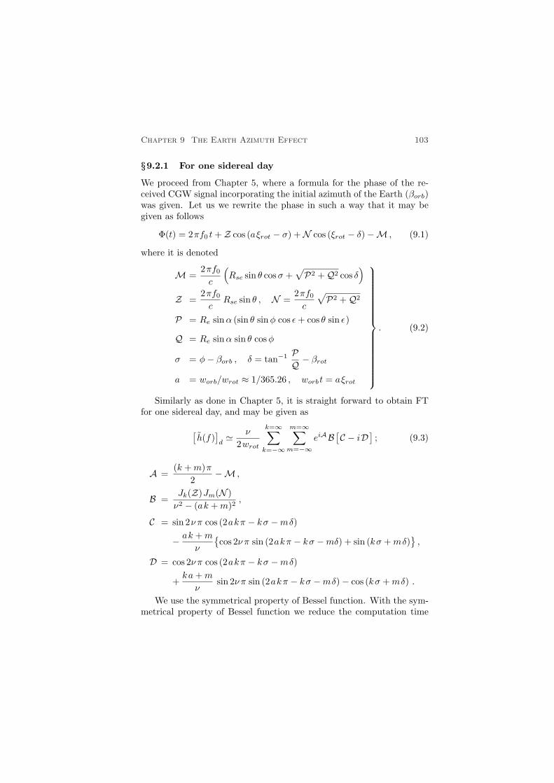
Chapter 9 The Earth Azimuth Effect 103
§9.2.1 For one sidereal day
We proceed from Chapter 5, where a formula for the phase of the re-ceived CGW signal incorporating the initial azimuth of the Earth (βorb)was given. Let us we rewrite the phase in such a way that it may begiven as follows
Φ(t) = 2πf0 t+ Z cos (aξrot − σ) +N cos (ξrot − δ)−M , (9.1)
where it is denoted
M =2πf0c
(Rse sin θ cosσ +
√P2 +Q2 cos δ
)
Z =2πf0c
Rse sin θ , N =2πf0c
√P2 +Q2
P = Re sinα (sin θ sinφ cos ε+ cos θ sin ε)
Q = Re sinα sin θ cosφ
σ = φ− βorb , δ = tan−1 PQ − βrot
a = worb/wrot ≈ 1/365.26 , worbt = aξrot
. (9.2)
Similarly as done in Chapter 5, it is straight forward to obtain FTfor one sidereal day, and may be given as
[h(f)
]d' ν
2wrot
k=∞∑
k=−∞
m=∞∑m=−∞
eiAB [C − iD ]; (9.3)
A =(k +m)π
2−M ,
B =Jk(Z)Jm(N )ν2 − (ak +m)2
,
C = sin 2ν π cos (2akπ − kσ −mδ)
− ak +m
ν
cos 2ν π sin (2akπ − kσ −mδ) + sin (kσ +mδ)
,
D = cos 2ν π cos (2akπ − kσ −mδ)
+ka+m
νsin 2ν π sin (2akπ − kσ −mδ)− cos (kσ +mδ) .
We use the symmetrical property of Bessel function. With the sym-metrical property of Bessel function we reduce the computation time
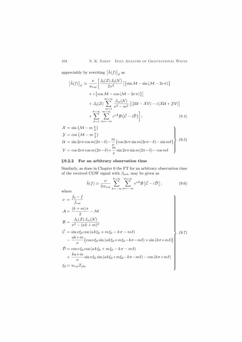
104 S. K. Sahay Data Analysis of Gravitational Waves
appreciably by rewriting[h(f)
]d
as
[h(f)
]d' ν
wrot
[J0(Z)J0(N )
2ν2
[sinM− sin (M− 2ν π)
+ icosM− cos (M− 2ν π)
]
+ J0(Z)m=∞∑m=1
Jm(N )ν2 −m2
[(YU − XV)− i(XU + YV)
]
+k=∞∑
k=1
m=∞∑m=−∞
eiAB( C − iD)]; (9.4)
X = sin(M−m π
2
)
Y = cos(M−m π
2
)
U = sin 2νπ cosm(2π−δ)−mν
cos 2νπ sinm(2νπ−δ)− sinmδ
V = cos 2νπ cosm(2π−δ)+m
νsin 2νπ sinm(2π−δ)− cosmδ
. (9.5)
§9.2.2 For an arbitrary observation time
Similarly, as done in Chapter 6 the FT for an arbitrary observation timeof the received CGW signal with βorb, may be given as
h(f) ' ν
2wrot
k=∞∑
k=−∞
m=∞∑m=−∞
eiAB [ C − iD ]; (9.6)
where
ν =f0 − f
frot
A =(k +m)π
2−M
B =Jk(Z)Jm(N )ν2 − (ak +m)2
C = sin νξ0 cos (akξ0 +mξ0 − kσ −mδ)
− ak+mν
cos νξ0 sin (akξ0+mξ0−kσ−mδ)+ sin (kσ+mδ)
D = cos ν ξ0 cos (akξ0 +mξ0 − kσ −mδ)
+ka+mν
sin νξ0 sin (akξ0+mξ0−kσ−mδ)− cos (kσ+mδ)
ξ0 = wrotTobs
. (9.7)
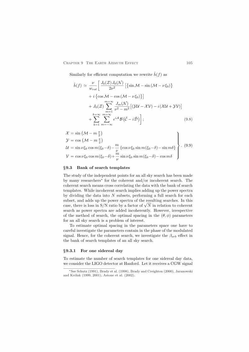
Chapter 9 The Earth Azimuth Effect 105
Similarly for efficient computation we rewrite h(f) as
h(f) ' ν
wrot
[J0(Z)J0(N )
2ν2
[sinM− sin (M− ν ξ0)
+ icosM− cos (M− ν ξ0)
]
+ J0(Z)m=∞∑m=1
Jm(N )ν2 −m2
[(YU − XV)− i(XU + YV)
]
+k=∞∑
k=1
m=∞∑m=−∞
eiAB(C − iD)]; (9.8)
X = sin(M−m π
2
)
Y = cos(M−m π
2
)
U = sin νξ0 cosm(ξ0−δ)−mνcos νξ0 sinm(ξ0−δ)− sinmδ
V = cos νξ0 cosm(ξ0−δ)+m
νsin νξ0 sinm(ξ0−δ)− cosmδ
. (9.9)
§9.3 Bank of search templates
The study of the independent points for an all sky search has been madeby many researchers∗ for the coherent and/or incoherent search. Thecoherent search means cross correlating the data with the bank of searchtemplates. While incoherent search implies adding up the power spectraby dividing the data into N subsets, performing a full search for eachsubset, and adds up the power spectra of the resulting searches. In thiscase, there is loss in S/N ratio by a factor of
√N in relation to coherent
search as power spectra are added incoherently. However, irrespectiveof the method of search, the optimal spacing in the (θ, φ) parametersfor an all sky search is a problem of interest.
To estimate optimal spacing in the parameters space one have tocareful investigate the parameters contain in the phase of the modulatedsignal. Hence, for the coherent search, we investigate the βorb effect inthe bank of search templates of an all sky search.
§9.3.1 For one sidereal day
To estimate the number of search templates for one sidereal day data,we consider the LIGO detector at Hanford. Let it receives a CGW signal
∗See Schutz (1991), Brady et al. (1998), Brady and Creighton (2000), Jaranowskiand Krolak (1999, 2001), Astone et al. (2002).

106 S. K. Sahay Data Analysis of Gravitational Waves
of a frequency of f0 =50 Hz from a source located at (θ, φ)= (0.1, 30).We chosen the data set such that βorb =0 at t= 0. In this case we takethe ranges of k and m as from 1 to 310 and from −10 to 10 respectivelyand the bandwidth equal to 2.0×10⁻³ Hz for the integration. Now, weselect the spacing 4θ=4.5×10⁻⁵, thereafter we maximize over φ byintroducing a spacing 4φ in the so obtained bank of search templatesand determine the resulting FF . In similar manner we obtain the FFat βorb = π
4and π
2. The results obtained are shown in Figure (9.1) and
the best fit of the graphs may be given as
Ntempl = 1015[c0+c1x−c2x2+c3x
3−c4x4+c5x5−c6x6+c7x
7]; (9.10)
0.80 6 x 6 0.995 ,
where c0, c1, c2, c3, c4, c5, c6, c7 are the constants which are given inTable (9.1).
In view of the above investigation, the grid spacing (4θ,4φ) in the(θ, φ)-parameter of templates may be expressed as
4θ = F(FF, f0, θ, φ, Tobs, βorb) . (9.11)Similarly,
4φ = G (FF, f0, θ, φ, Tobs, βorb) . (9.12)
In Chapter 7, for one sidereal data set, the dependence of FF onthe template variables θT and φT is given as
FF = e−0.00788(θ−θT )2 . (9.13)
FF = e−0.01778(φ−φT )2 . (9.14)
From Eqs. (9.11), (9.19), (9.13), and (9.20), we may write
F(FF, 50, 0.1, 30, 1d, βorb) =[−(0.00788)−1 ln(FF )
]1/2, (9.15)
G (FF, 50, 0.1, 30, 1d, βorb) =[−(0.01778)−1 ln(FF )
]1/2. (9.16)
Hence, for the selected FF one can determine4θ and4φ. However,there is no unique choice for it.
§9.3.2 For one week
In this case, we consider the LIGO detector at Livingston which is get-ting a CGW signal of a frequency f0 =50 Hz from a source located at(θ, φ)= (1, 45). First, we chosen the data set such that βorb =0 at
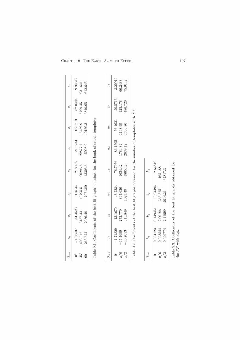
Chapter 9 The Earth Azimuth Effect 107
βorb
c 0c 1
c 2c 3
c 4c 5
c 6c 7
0
−4.3
6537
34.4
523
116.4
4218.4
62
245.7
34
165.7
19
62.0
404
9.9
4642
45
−403.0
12
3187.4
410795.5
20296.6
22877.7
15459.9
5799.4
5931.6
41
90
−263.6
22
2086.4
87071.8
013305.6
15008.9
10150.3
3810.6
5612.6
45
Table
9.1
:C
oeffi
cien
tsofth
ebes
tfit
gra
phs
obta
ined
for
the
bank
ofse
arc
hte
mpla
tes.
βorb
a0
a1
a2
a3
a4
a5
a6
a7
0−1
.71829
13.1
670
43.2
234
78.7
956
86.1
505
56.4
921
20.5
716
3.2
0919
π/6
−35.7
699
273.7
70
897.6
36
1634.4
21784.8
41168.9
9425.1
78
66.2
488
π/2
−40.7
053
311.8
49
1023.4
91865.4
22039.1
21336.8
6486.7
20
75.9
142
Table
9.2
:C
oeffi
cien
tsofth
ebes
tfit
gra
phs
obta
ined
for
the
num
ber
ofte
mpla
tes
wit
hF
F.
βorb
b 0b 1
b 2b 3
00.9
94123
0.1
49451
3.9
4494
2.6
4819
π/6
0.9
93544
2.0
0186
366.3
75
1651.8
8
π/2
0.9
96774
2.1
1099
2914.2
137817.3
Table
9.3
:C
oeffi
cien
tsof
the
bes
tfit
gra
phs
obta
ined
for
the
FF
wit
h4
φ.

108 S. K. Sahay Data Analysis of Gravitational Waves
Figure 9.1: Variation in the number of search templates with FF at at differentvalues of βorb.
t=0. In this case we take the ranges of k and m as from 1 to 2800 andfrom −15 to 15 respectively and the bandwidth equal to 50± 3.28×10⁻⁴
Hz for the integration. Now, we select the spacing 4θ=0.45×10⁻⁴,thereafter we maximize over φ by introducing a spacing 4φ in the soobtained number of templates and determine the resulting FF . In sim-ilar manner we obtain the number of templates for βorb = π
6and π
2. The
results obtained are shown in Fig. (9.2). We also plot the templatesspacing 4φ in the φ-parameter with FF shown in Fig. (9.3) and thebest fit of curves may be given as
Ntempl = 1018[a0+a1x−a2x
2+a3x3−a4x
4+a5x5−a6x
6+a7x7]; (9.17)
0.85 6 x 6 0.995;
FF = b0 + b1y − b2y2 + b3y
3; 0.037 6 y 6 0.69; (9.18)
where a0 . . . a7 and b0 . . . b3 are constants as given in Table (9.2) and(9.3) respectively.
In view of the above investigation, the spacing4φ in the φ-parametermay be expressed as
4φ = G (FF, f0, θ, φ, Tobs, βorb) . (9.19)
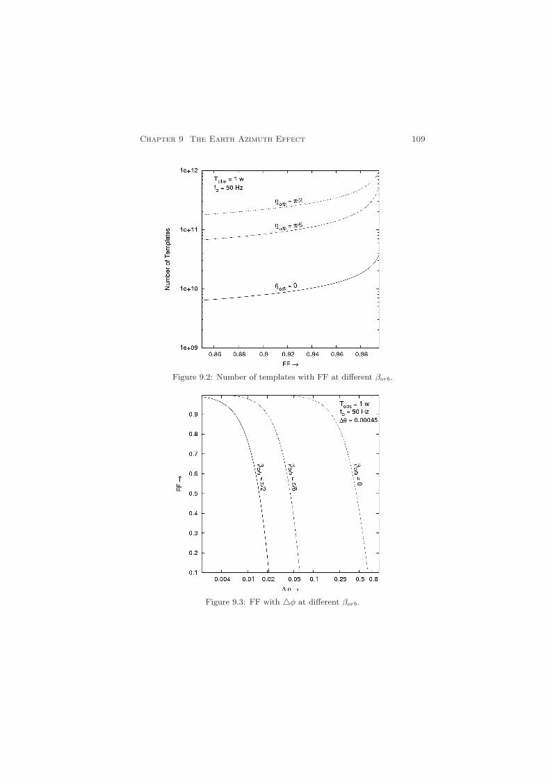
Chapter 9 The Earth Azimuth Effect 109
Figure 9.2: Number of templates with FF at different βorb.
Figure 9.3: FF with 4φ at different βorb.
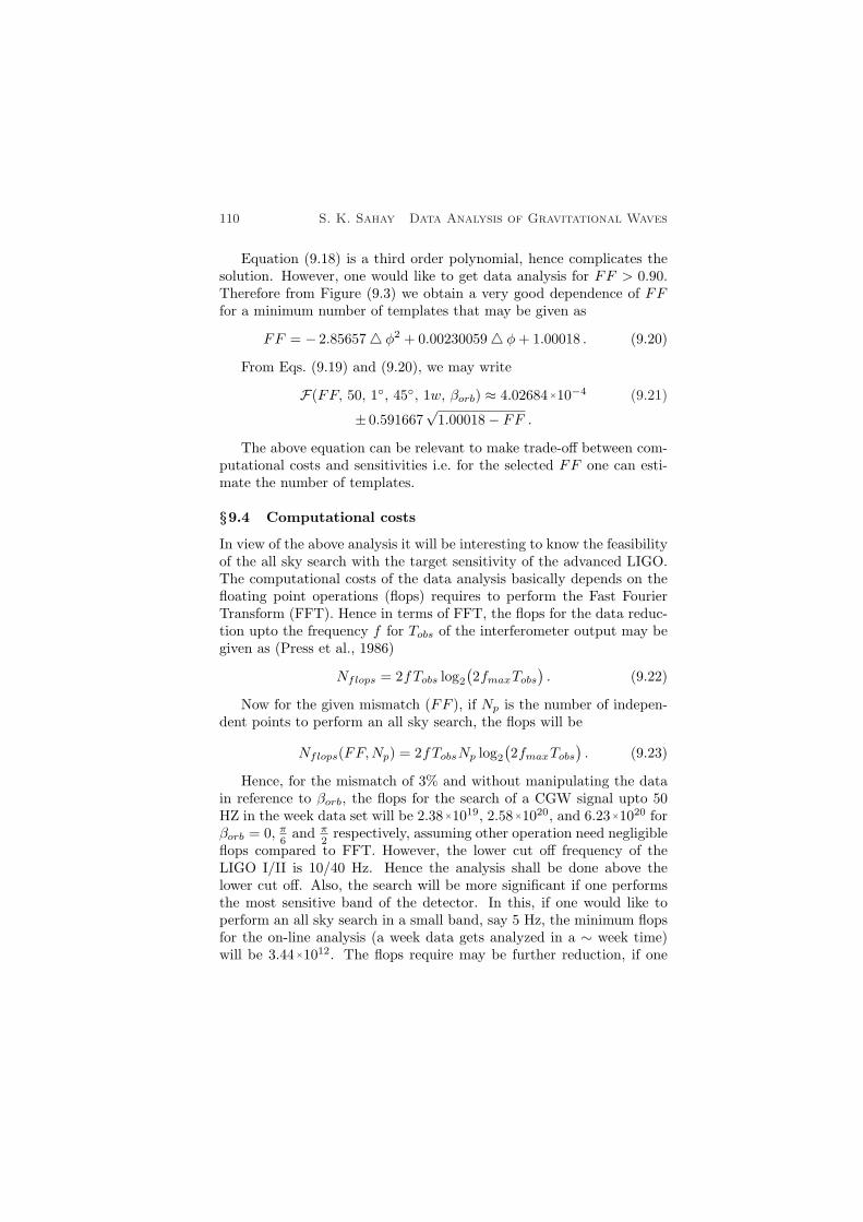
110 S. K. Sahay Data Analysis of Gravitational Waves
Equation (9.18) is a third order polynomial, hence complicates thesolution. However, one would like to get data analysis for FF > 0.90.Therefore from Figure (9.3) we obtain a very good dependence of FFfor a minimum number of templates that may be given as
FF = − 2.856574 φ2 + 0.002300594 φ+ 1.00018 . (9.20)
From Eqs. (9.19) and (9.20), we may write
F(FF, 50, 1, 45, 1w, βorb) ≈ 4.02684×10⁻⁴ (9.21)
± 0.591667√
1.00018− FF .
The above equation can be relevant to make trade-off between com-putational costs and sensitivities i.e. for the selected FF one can esti-mate the number of templates.
§9.4 Computational costs
In view of the above analysis it will be interesting to know the feasibilityof the all sky search with the target sensitivity of the advanced LIGO.The computational costs of the data analysis basically depends on thefloating point operations (flops) requires to perform the Fast FourierTransform (FFT). Hence in terms of FFT, the flops for the data reduc-tion upto the frequency f for Tobs of the interferometer output may begiven as (Press et al., 1986)
Nflops = 2fTobs log2
(2fmaxTobs
). (9.22)
Now for the given mismatch (FF ), if Np is the number of indepen-dent points to perform an all sky search, the flops will be
Nflops(FF,Np) = 2fTobsNp log2
(2fmaxTobs
). (9.23)
Hence, for the mismatch of 3% and without manipulating the datain reference to βorb, the flops for the search of a CGW signal upto 50HZ in the week data set will be 2.38×10¹⁹, 2.58×10²⁰, and 6.23×10²⁰ forβorb = 0, π
6and π
2respectively, assuming other operation need negligible
flops compared to FFT. However, the lower cut off frequency of theLIGO I/II is 10/40 Hz. Hence the analysis shall be done above thelower cut off. Also, the search will be more significant if one performsthe most sensitive band of the detector. In this, if one would like toperform an all sky search in a small band, say 5 Hz, the minimum flopsfor the on-line analysis (a week data gets analyzed in a ∼ week time)will be 3.44×10¹². The flops require may be further reduction, if one
Chapter 9 The Earth Azimuth Effect 111
performs a hierarchical search. Hence, it may be feasible to perform alimited frequency all sky search of a signal amplitude & 10−26 in theoutput of such a sensitive detector with a TFLOPS computer.
§9.5 Summary
The initial azimuth of the Earth has been incorporated in the FT ofthe frequency modulated signal, and its effect in the bank of templatesrequired for the search of CGW in an all sky search is discussed. Inthe investigation for one sidereal day data set of a signal of 50 Hz, weobserve that the number of search templates varies significantly withβorb. From the analysis we found that for FF =0.97 approximately24.8267×1010, 22.7840×10¹², and 32.3097×10¹² search templates maybe required, if βorb = 0, π
4and π
2respectively.
Similarly, the number of search templates for the search in the out-put of one week data set. We observe that for FF =0.97 there approx-imately 1.53×10¹⁰, 1.66×10¹¹, and 4.0×10¹¹ templates will be requiredwhen βorb =0, π
6and π
2respectively. Hence, the analysis may be useful
to reduce the computational cost for a coherent all sky search. However,also the inspection of the phase of the modulated signal reveals that thereduction in the bank of search templates depends on the time scale ofintegration, shorter than Tobs, resulting more difference in the numberof templates.
The reduction in the number of templates is large, so we studied thefeasibility of all sky search in reference to the advanced LIGO and foundthat in the band of 5 Hz one may perform an on-line all sky search ofa CGW signal of an amplitude of & 10−26 with a TFLOPS computer.The relation given by Equation (9.22) may be useful to make trade-offbetween computational costs and sensitivities for the search of CGW.The issue to reduce the flops for all sky search is a problem of interestsand hence needs more studies.

Bibliography
1. Abramovici A., Althouse W.E., Drever R.W.P., Gursel Y., Kanwa-mura S., Raab F.J. Shoemaker D., Sievers L., Spero R.E., Thorne K.S.,Vogt R.E., Weiss R., Whitcomb S.E., and Zucker Z.E. Science, 1992,v. 256, 325.
2. Abrmowitz M. and Stegun I.A. In: Handbook of Mathematical Functions,Dover Publication, New York, 10th printing with corrections of first edi-tion, 1972.
3. Allen B. In: Relativistic Gravitation and Gravitational Radiation, ed.by Marck J.A. and Lasota J.P, Cambridge University Press, Cambridge,1997.
4. Andersson N. Astrophys. J., 1998, v. 502, 708.
5. Apostolatos T.A. Phys. Rev. D, 1995, v. 52, 605.
6. Apostolatos T.A. Phys. Rev. D, 1996, v. 54, 2421.
7. Astone P., Borkowski K.M., Jaranowski P. and Krolak A. Phys. Rev. D,2002, v. 65, 042003.
8. Bildsten L. Astrophys. J. Lett., 1998, v. 501, L89.
9. Blair D. and Ju L. Monthly Not. RAS, 1996, v. 283, 648.
10. Blair D.G. In: Gravitational Wave Data Analysis, ed. by Schutz B.F.,Kluwer Press, Dordrecht, 1989.
11. Blair D.G. In: The Detection of Gravitational Waves, ed. by Blair D.G.Cambridge University Press, Cambridge, England, 1991.
12. Bonazzola S. and Gourgoulhon E. Astron. and Astrophys., 1996, v. 312,675.
13. Bradaschia C., Calloni E., Cobal M., Fabbro R.D., Virgilio A.D., Gia-zotto A., Holloway L.E., Kautzky H., Michelozzi B., Montelatici V., Pas-suello D., and Velloso W. In: Gravitation 1990, Proceedings of the BanffSummer Institute, edited by Mann R. and Wesson P. World Scientific,Singapore, 1991.
14. Brady P.R., Creighton T., Cutler C., and Schutz B.F. Phys. Rev. D, 1998,v. 57, 2101.
15. Brady P.R. and Creighton T. Phys. Rev. D, 2000, v. 61, 082001.
16. Bracewell Ron. The Fourier Transform and Its Application. 2nd revisededition, McGraw-Hill, New York, 1984.
17. Brigham E.O. The Fast Fourier Transform and its Application. Prentice-Hall International, 1988.
18. Cutler C., Apostolatos T.A., Bildsten L., Finn L.S., Flanagan E.E.,Kennefick D., Markovic D.M., Ori A., Poisson E., Sussman G.J. andThorne K.S. Phys. Rev. Lett., 1993, v. 70, 2984.

Bibliography 113
19. Damour T. Three Hundred Years of Gravitation. Ed. by Hawking S.W.and Israel W., Cambridge University Press, Cambridge, England, 1987.
20. Damour T. In: Gravitation in Astrophysics, ed. by Carter B. and HartleJ.B., Plenum Press, New York, 1987.
21. Danzmann K. In: Gravitational Wave Experiment, ed. by Coccia E.,Pizzela G., and Ronga F., World Scientific, Singapore, 1995, 100–111.
22. Dhurandhar S.V. and Sathyaprakash B.S. Phys. Rev. D, 1994, v. 49, 1707.
23. Frasca S. Int. J. Mod. Phys. D., 2000, v. 9, 369.
24. Giazotto A., Bonazzola S., and Gourgoulhon E. Phys. Rev. D, 1997, v. 55,2014.
25. Goldstein H. Classical Mechanics. Addison-Wesley, New York, 1980.
26. Green R.M. Spherical Astronomy. Cambridge University Press, Cam-bridge, England, 1985.
27. Grishchuk L.P. Class. Quant. Gravity, 1997, v. 14, 1445.
28. Helstrom C.W. Statistical Theory of Signal Detection. 2nd ed., PergamonPress, London, 1968.
29. Hough J. In: Gravitational Wave Experiment, ed. by Coccia E., Pizze-la G., and Ronga F., World Scientific, Singapore, 1995, 50–63.
30. Hulse R.A. and Taylor J.H. Astrophys. J. Lett., 1975, v. 195, L51–L53.
31. Jaranowski P., Krolak A., and Schutz B.F. Phys. Rev. D, 1998, v. 58,063001.
32. Jaranowski P. and Krolak A. Phys. Rev. D, 1999, v. 59, 063003.
33. Jaranowski P. and Krolak A. Phys. Rev. D, 2000, v. 61, 062001.
34. Jotania K. and Dhurandhar S.V. Bull. Astron. Soc. India, 1994, v. 22,303.
35. Jotania et al. Astron. and Astrophys., 1996, v. 306, 317–325.
36. Kulkarni S.R. Philos. Trans. R. Soc. London, 1992, v. 341, 77.
37. Krolak A. In Gravitational Wave Data Analysis, ed. by Schutz B.F.,Kluwer Press, Dordrecht, 1989.
38. Landau L.D. and Lifshitz E.M. Mechanics. Pergamon Press, Oxford, Eng-land, 1969.
39. Landau L.D. and Lifshitz E.M. The Classical Theory of Fields. PergamonPress, Oxford, England, 1975.
40. Lindblom L., Owen B.J., and Morsink S.M. Phys. Rev. Lett., 1998, v. 80,4843.
41. Manchester R.N. Philos. Trans. R. Soc. London, 1992, v. 341, 3.
42. McCleland et al. In: Proceedings of the 3rd Edoardo Amaldi Conference,ed. by S. Meshkov, AIP Conference Proceedings, v. 523, 140, Melville,New York, 2000.
43. Misner C.W., Thorne K.S., and Wheeler J.A. Gravitation. W.H. Freemanand Company, San Francisco, 1973.
44. Mohanty S.D. and Dhurandhar S.V. Phys. Rev. D, 1996, v. 54, 7108.
45. Mohanty S.D. Phys. Rev. D, 1998, v. 57, 630.
114 S. K. Sahay Data Analysis of Gravitational Waves
46. Narayan R., Piran T., and Shemi A. Astrophys. J. Lett., 1991, v. 379,L17.
47. Owen B.J. Phys. Rev. D, 1996, v. 53, 6749.
48. Owen B.J. and Sathyaprakash B.S. Phys. Rev. D, 1999, v. 60, 022002.
49. Owen B.J., Lindblom L., Cutler C., Schutz B.F., Vecchio A., and Ander-sson N. Phys. Rev. D, 1998, v. 58, 084020.
50. Pandharipande V.R., Pines D., and Smith R.A. Astrophys. J., 1976,v. 208, 550.
51. Papoulis A. Signal Analysis. McGraw-Hill Inc., Singapore, 1977.
52. Phinney E.S. Astrophys. J. Lett., 1991, v. 330, L17.
53. Press W.H., Flannery B.P., Teukoslsky S.A., and Vetterling W.T. Numer-ical Recipes: The Art of Scientific Computing. Cambridge Univ. Press,Cambridge, 1986.
54. Sahay S.K. Int. J. Mod. Phys. D., 2003, v. 12, no. 7, 1227.
55. Sahay S.K. Int. J. Mod. Phys. D., 2006, v. 15, no. 2, 225.
56. Saulson P.R. Fundamentals of Interfeometric Gravitational Wave Detec-tors. World Scientific Publishing, Singapore, 1994.
57. Sathyaprakash B.S. and Dhurandhar S.V. Phys. Rev. D, 1991, v. 44, 3819.
58. Sathyaprakash B.S. In: Black Holes, Gravitational Radiation and theUniverse, ed. by Iyer B.R. and Bhawal B., Kluwer Press, Dordrecht, 1999.
59. Schutz B.F., Davier M., and Hello P., eds. Proceedings of GravitationalWave Data Analysis Workshop, Orsay, France 1997, Editions Frontieres,Paris, 113–143.
60. Schutz B.F. Class. Quant. Gravity, 1993, v. 10, 135.
61. Schutz B.F. Class. Quant. Gravity, 1999, v. 16, A131.
62. Schutz B.F. and Tinto M. Monthly Not. RAS, 1987, v. 224, 131.
63. Schutz B.F. The Detection of Gravitational Waves. Ed. by Blair, D.G.,Cambridge University Press, Cambridge, England, 1991.
64. Schutz B.F. A First Course in General Relativity. Cambridge UniversityPress, Cambridge, England, 1989.
65. Shanmugam K.S. and Breiphol A.M. Random Signals: Detection, Esti-mation and Data Analysis. Willey, New York, 1989.
66. Smart W.M. In: Textbook on Spherical Astronomy, Cambridge UniversityPress, Cambridge, 1977.
67. Srivastava D.C. and Sahay S.K. Monthly Not. RAS, 2002, v. 337, 305.
68. Srivastava D.C. and Sahay S.K. Monthly Not. RAS, 2002, v. 337, 315.
69. Srivastava D.C. and Sahay S.K. Monthly Not. RAS, 2002, v. 337, 322.
70. Tagoshi H., Kanda N., Tanaka T., Tatsumi D., Telada S., Ando M.,Arai K., Araya A., Asada H., et al. Phys. Rev. D, 2001, v. 63, 062001.
71. Tsubona K. In: Gravitational Wave Experiment, ed. by Coccia E., Pizze-la G., and Ronga F., World Scientific, Singapore, 1995, 112–114.
72. Thorne K.S. In: Three Hundred Years of Gravitation, ed. by Hawk-ing S.W., Israel W., Cambridge University Press, Cambridge, 1987.

Bibliography 115
73. Weber J. Phys. Rev., 1960, v. 117, 306.
74. Weinstein A. Class. Quant. Gravity, 2002, v. 19, 1575–1584.
75. Weiss R. Reviews of Modern Physics, 1999, v. 71, 187.
76. Zimmermann M. and Szedenits E. Phys. Rev. D, 1979, v. 20, 351.
77. Zimmermann M. Phys. Rev. D, 1980, v. 21, 891.

About the author
Sanjay Kumar Sahay (b. 1970 in East Singhbhum, India) was educatedfrom Ranchi University, India. He obtained PhD in data analysis ofgravitational waves from D.D.U. Gorakhpur University, India, in 2003.After submission of PhD, during 2002–2003, he continued his work ongravitational waves at Inter University Centre for Astronomy and Astro-physics, Pune, India. In 2003–2005 he worked on the multi-wavelengthastronomy project, ASTROSAT at Raman Research Institute, Banga-lore, India. On 2005 he worked as post doctoral fellow at Tel AvivUniversity, Israel, with the ultra violet detector TAUVEX (Tel AvivUniversity Ultra-violet Explorer), under training of Prof. Noah Brosch.Commencing in December, 2005, he is joined as a lecturer in Birla In-stitute of Technology and Science, Pilani — Goa Campus, India, and isstill working independently on gravitational waves.
Svenska fysikarkivet books
A Revised Electromagnetic Theory with FundamentalApplications by Bo LehnertSvenska fysikarkivet, 2008, 158 pages. ISBN 978-91-85917-00-6
Summary: There are important areas within which the conventional electromag-netic theory of Maxwell’s equations and its combination with quantum mechanicsdoes not provide fully adequate descriptions of physical reality. As earlier pointedout by Feynman, these difficulties are not removed by and are not directly asso-ciated with quantum mechanics. Instead the analysis has to become modified inthe form of revised quantum electrodynamics, for instance as described in this bookby a Lorentz and gauge invariant theory. The latter is based on a nonzero electriccharge density and electric field divergence in the vacuum state, as supported bythe quantum mechanical vacuum fluctuations of the zero-point energy. This theoryleads to new solutions of a number of fundamental problems, with their applicationsto leptons and photon physics. They include a model of the electron with its point-charge-like nature, the associated self-energy, the radial force balance in presenceof its self-charge, and the quantized minimum value of the free elementary charge.Further there are applications on the individual photon and on light beams, in re-spect to the angular momentum, the spatially limited geometry with an associatedneedle-like radiation, and the wave-particle nature in the photoelectric effect and intwo-slit experiments.
Spin-Curvature and the Unification of Fieldsin a Twisted Space by Indranu SuhendroSvenska fysikarkivet, 2008, 78 pages. ISBN 978-91-85917-01-3
Summary: The book draws theoretical findings for spin-curvature and the uni-fication of fields in a twisted space. A space twist, represented through the ap-propriate formalism, is related to the anti-symmetric metric tensor. Kaluza’s the-ory is extended and given an appropriate integrability condition. Both matter andthe isotropic electromagnetic field are geometrized through common field equations:trace-free field equations giving the energy-momentum tensor for such an electromag-netic field solely via the (generalized) Ricci curvature tensor and scalar are obtained.In the absence of electromagnetic fields the theory goes to Einstein’s 1928 theoryof distant parallelism where only matter field is geometrized (through the twist ofspace-time). The above results in common with respective wave equations are joinedinto a “unified field theory of semi-classical gravoelectrodynamics”.
Particles Here and Beyond the Mirrorby D.Rabounski and L.BorissovaSvenska fysikarkivet, 2008, 118 pages. ISBN 978-91-85917-03-7
Summary: This is a research on all kinds of particles, which could be conceivablein the space-time of General Relativity. In addition to mass-bearing particles andlight-like particles, zero-particles are predicted: such particles can exist in a fullydegenerate space-time region (zero-space). Zero-particles seems as standing light
118 S. K. Sahay Data Analysis of Gravitational Waves
waves, which travel in instant (non-quantum teleportation of photons); they mightbe observed in a further development of the “stopped light experiment” which wasfirst conducted in 2001, at Harvard, USA. The theoretical existence of two separateregions in the space-time is also shown, where the observable time flows into the fu-ture and into the past (our world and the mirror world). These regions are separatedby a space-time membrane wherein the observable time stops. A few other certainproblems are considered. It is shown, through Killing’s equations, that geodesic mo-tion of particles is a result of stationary geodesic rotation of the space which hoststhem. Concerning the theory of gravitational wave detectors, it is shown that bothfree-mass detector and solid-body detector may register a gravitational wave only ifsuch a detector bears an oscillation of the butt-ends.
Data Analysis of Gravitational Waves by S.K. SahaySvenska fysikarkivet, 2008, 118 pages. ISBN 978-91-85917-05-1
Summary: The detection of GW in the noisy output of the detectors has its ownproblem, not the least of which is the sheer volume of data analysis. The data anal-ysis of the signals is computationally demanding even for the standard computerexpected to be available in the near future. Hence, the book discusses the dataanalysis problem of the signal by developing the analytical Fourier Transform withtaking into account the Earth’s rotational motion around its axis, and its revolutionaround the Sun for efficient data analysis, efficient not only in a picking weak signalfrom the noisy data but also in terms of the computing-cost. Taking the advanatageof the analytical Fourier Transform over the Fast Fourier Transform in terms of reso-lution and computational cost, we applied the technique of ”Matched Filtering” andesitmated the number of templates required for matched filtering in an all sky searchof the signal, and also an analysis has been done for the possible symmetries in thesky location as the parameters of the signal manifold and templates correspondingto the different source locations. The trade-off between computational cost and sen-sitivies arises due the Earth azimuth in the bank of search templates for an all-skysearch of the singal has been also discussed.
Data Analysis of Gravitational Waves by S. K. Sahay
The detection of GW in the noisy output of the detectors has its own problem, notthe least of which is the sheer volume of data analysis. The data analysis of thesignals is computationally demanding even for the standard computer expected tobe available in the near future. Hence, the book discusses the data analysis prob-lem of the signal by developing the analytical Fourier Transform with taking intoaccount the Earth’s rotational motion around its axis, and its revolution around theSun for efficient data analysis, efficient not only in a picking weak signal from thenoisy data but also in terms of the computing-cost. Taking the advantage of theanalytical Fourier Transform over the Fast Fourier Transform in terms of resolutionand computational cost, we applied the technique of “Matched Filtering” and es-timated the number of templates required for matched filtering in an all sky searchof the signal, and also an analysis has been done for the possible symmetries in thesky location as the parameters of the signal manifold and templates correspondingto the different source locations. The trade-off between computational cost andsensitivities arises due the Earth azimuth in the bank of search templates for anall-sky search of the singal has been also discussed.
Databehandling av gravitationsvagor av S. K. Sahay
Att kunna isolera gravitationsvagor vid hog brusniva hos detektorn ar forknippadmed en del problem, inte minst med tanke pa de stora berakningsvolymerna sombehovs for dataanalysen. Analysen av alla data och sjalva signalen ar mycketkravande, aven for en standarddator, som forvantas vara tillganglig inom narmasteframtiden. I boken behandlas dataanalysproblemet genom utveckling av en ana-lytisk Fourier transform som tar hansyn till Jordens rotation runt egen axel och runtsolen. Genom detta forbattras mojligheten att isolera den svaga signalen med enmycket lagre datorkapacitet, an det som annars hade behovts. Genom att anvandasig av de fordelar som den analytiska Fourier trasformen, jamfort med FFT, ger ifraga av upplosning och berakningskostnader, vi tillampade en teknik som vi kallar”anpassad filtrering” for att fa en uppskattning pa antalet mallar som behovs foranpassad filtrering i en omfattande avsokning av himlen. En kompromiss mel-lan berakningskostnaderna och kanslighet som uppkommer inom sokmallbankenberoende av Jordens azimut vid en omfattande avsokning efter signalen har ocksadiskuterats i boken.
Svenska fysikarkivet, Stockholm, 2008, 118 pages
![Abstract arXiv:1903.11752v2 [cs.CV] 26 Jul 2019Real-time generic object detection. Real-time object de-tection is another important problem for CNN-based detec-tors. Commonly, one-stage](https://static.documents.pub/doc/80x56/5f23e87ada8c6c3b1323d815/abstract-arxiv190311752v2-cscv-26-jul-2019-real-time-generic-object-detection.jpg)


