Data Anonymisation and Risk Assessment Automation

Data Anonymisation and Risk Assessment Automation

1 | PHUSE Deliverables

Data Anonymisation and Risk Assessment

Automation

phuse.eu



Contents

Definitions 1

Introduction 1

Anonymisation Process 2

1 Gather Original Data 2 1 1 Identify source data, specifications, formats 2

2 Pre-Process Data 2 2 1 Prepare study datasets to create standard input data 2

3 Find Potential Direct and Quasi-identifiers 2 3 1 Find identifiers using the PHUSE De-identification

Standard for SDTM 2 3 2 Find identifiers by variable name and content 6 3 2 1 Subject IDs Site, lab, test, reference IDs 6 3 2 2 Date and time variables 6 3 2 3 Demographic and baseline characteristics 6 3 2 4 Birth/death dates 6 3 2 5 Verbatim terms and free-entry (comments)

variables 6 3 2 6 Values (sex, age, race, dates, etc ) within result

qualifier variables 7 3 2 7 Sensitive information (pregnancy, abortions,

mental health, family, etc ) 7 3 2 8 Rare diseases reported in Adverse Event &

Medical History data 7

4 Define De-identification Rules, Build Specifications 7 4 1 Dataset-level rules 7 4 1 1 KEEP – keep variable as is 7 4 1 2 DROP – remove variable 8 4 1 3 CLEAR – keep variable but leave empty 8 4 1 4 NEW – add variable 8 4 2 ID variables 8 4 2 1 RECODE_ID (var, key) – replace/recode ID value 8 4 3 Date variables 10 4 3 1 Study days (relative to the reference start date) 10 4 3 2 OFFSET (var, offset, partial) 10 4 4 Age variables 10 4 4 1 AGE_BANDS (var, size, start) 11 4 4 2 AGE_IN_BAND (var, start, size) 12 4 4 3 AGE90 (var) 12 4 5 Categorical variables 13 4 5 1 COUNTRY_POOL (var, country) 13 4 5 2 LOW_FREQ_POOL (var, proportion) 13 4 5 3 REDACT (var, redact_values) 14 4 6 Vertical datasets 15

5 Calculate Residual Risk of Re-identification 15 5 1 Risk of re-identification attempt being made 15 5 1 1 Deliberate attack 15 5 1 2 Inadvertent re-identification (recognition) 15 5 1 3 Data breach 16 5 1 4 Public data release 16 5 2 Selecting quasi-identifiers for calculating the risk

of success 16 5 3 Base Dataset for calculating risk 16 5 4 Risk of successful re-identification (assuming attempt

has taken place) 16 5 4 1 Individual risk of re-identification for each subject

in the dataset 16

5 4 2 Average and maximum risk across all records of a dataset 17

5 4 3 Calculating the risk on a subset of records 17 5 5 Reference population 19 5 6 Overall risk of re-identification 19 5 7 k-anonymity and uniqueness 20 5 8 Threshold 20 5 8 1 Risk threshold 20 5 8 2 “Uniqueness” threshold 20

6 Apply De-identification Rules to Dataset 20 6 1 The first scenario 20 6 2 Apply the de-identification rules 20 6 3 Multiple de-identification scenarios – Rule Dataset 21 6 4 Testing all scenarios 22 6 5 Optimal scenario 24 6 6 Data utility/information loss metrics 24 6 7 Transform all datasets 24 6 8 Convert anonymised datasets to desired format 24 6 9 Compile the anonymised package 24

7 Anonymisation Report 24

Process in a Nutshell 25

References and Literature 26

Acknowledgements 26




Definitions

Data SubjectIndividual participant in a clinical study

Subject Level DataData linked to and describing data subjects, stored in one or many datasets

Identifiable DataSubject level data which can be linked to an identifiable natural person directly or indirectly, in particular by reference to details such as name, identification number, location data or to one or more factors specific to the physical, physiological, genetic, mental, economic, cultural or social identity of that natural person

Data Controller/SponsorOrganisation responsible for collecting, storing, and processing the original subject level data, as well as preparing data for sharing with data requestors

Data Requestor/Data RecipientOrganisation or person requesting access to data from the data controller to use it for their own purposes

De-identification/AnonymisationProcess of modifying data in such a way that it is deemed no longer identifiable, ensuring the risk of re-identification of any study subject, by all means reasonably likely to be used, is small The meaning of the two terms may be nuanced in different jurisdictions and settings

Within this document, “de-identification” applies to the action of transforming directly or indirectly identifying details or variables in order to reduce/remove their association with data subjects “Anonymisation” is used to describe the overall process of modifying data It contains selecting identifiers and rules, de-identifying multiple variables, assessing and controlling residual re-identification risk

PseudonymisationProcess of replacing real values with “fake” values (pseudonyms), applied in a manner that is random, consistent, and irreversible

Re-identificationEvent (deliberate or inadvertent) of correctly associating subject level data with one or many data subjects

Direct IdentifierDetail which can be used to uniquely identify an individual, e g Subject ID, Social Security Number, Telephone Number, Exact Address It is compulsory to remove or de-identify any direct identifier

Quasi-identifier/Indirect IdentifierBackground detail in data which can be used in connection with other information to identify an individual with a high probability, e g age at baseline, race, sex, rare event, specific finding

Doc ID: WP-045 Version: 1.0 Working Group: Data Transparency Date: 09-June-2020

Base DatasetDataset based on which re-identification risk is calculated Contains one record for each participant of the trial, containing direct and quasi-identifiers

Equivalence ClassA group of subjects or records sharing the same values of quasi-identifiers, e g 28-year-old females in Australia

Prosecutor riskA method of calculating risk based solely on the records present in the Base Dataset Equivalence classes are constructed only using records in the Base Dataset

Journalist riskA method of calculating risk based on populations larger than the Base Dataset Equivalence classes are constructed using records from additional sources

Introduction

Sharing clinical trial data and results is an increasingly important topic Making sure that, prior to sharing, data is anonymised and transformed in a way that protects identity of subjects while retaining utility for researchers has never been more relevant The objective of this document is to draw a detailed dataset(s) anonymisation process map, identify challenges and potential pitfalls of the process, suggest best practices and offer automation ideas and examples The basis for the discussions is the quantitative approach to risk assessment – where risk is calculated (as opposed to being qualified)

The paper discusses scenarios in which data is being shared on request and with typical controls in place (e g Data Sharing Agreement, access restrictions), but the proposed approach can be extrapolated with careful considerations to public release of data

It focuses on sharing and anonymising subject level datasets (in tabular form) Anonymisation and redaction of clinical documents is not in scope of this paper

All code examples are offered in SAS®, Python, R, and (in a few cases) Julia It was important to the authors to focus on the algorithm, without being tied to any particular tool The languages have different programming paradigms and providing parallel examples should allow the reader to choose the option that best suits them

The code examples in this document are provided without any warranty of being correct or fit for the reader’s individual purposes They serve as illustrations of possible approaches and it is the reader’s responsibility to adapt and validate the code for their own usage against clinical data



Anonymisation Process

1. Gather Original Data

1.1. Identify source data, specifications, formats

Before any anonymisation work can commence, source data needs to be identified It is helpful to understand the relationships between datasets and their structure Data may be stored across different locations and in different formats It is essential to identify the correct copy/cut-off of the data and the structure most appropriate to the tools which will be used for processing When using SAS®, especially regarding legacy data, it’s important to identify any formats which may be stored in a separate SAS® catalog so that they can be applied in the later steps and any coded values can be properly formatted and decoded

Datasets in other formats may be accompanied by metadata datasets, containing variable/column attributes (labels, type, length, etc ) Those may prove helpful in processing data and producing output datasets

It is also useful to collect all relevant supporting documentation, e g data entry annotations, mapping specifications, derived datasets specifications such as Define-XML

3. Find Potential Direct and Quasi-identifiers

3.1. Find identifiers using the PHUSE De-identification Standard for SDTM

When working with SDTM datasets, the first step of finding direct and quasi-identifiers should be to check the variables against the PHUSE De-identification Standard for SDTM to find identifiers and corresponding rules This will help find direct and quasi-identifiers, as well as recommended de-identification rules to apply to the discovered identifiers

To achieve this, merge the table containing input dataset specifications containing the list of datasets/variables with the PHUSE Standard spreadsheet

2. Pre-Process Data

2.1. Prepare study datasets to create standard input data

Pre-processing data at the early stage may identify and remove issues which can potentially affect the process in later stages CDISC data (SDTM, ADaM) follows strict specification which makes manipulation (e g transforming, combining) easier, but legacy data can follow different, often inconsistent, rules which are best dealt with early in the anonymisation process

For various reasons (e g legal) some subjects’ data may not be shared In such cases relevant subjects and related subject level data will need to be removed from the anonymised dataset, but they can still be used for risk calculations

It is worth addressing the following issues before any further processing:

• Ensure consistent key variable/subject ID. Each dataset containing subject level information must include a key variable/subject ID that is the same between datasets

• Ensure each variable name has unique data type. Variables in different datasets may share a name but have different attributes (AGE can be a numeric variable in one dataset and a character one in another) This can cause serious problems with standard macros expecting specific data types and can lead to mapping issues Consider converting inconsistent variables to the same type

• Remove SAS® formats. Replace any variables with an assigned format to a decoded

The same data may be present in the raw version, SDTM and ADaM structure Confirm which is the relevant variant When more than one, check the information is consistent

• SAS® format may be stored in a separate catalog, without which the data may be hard to read and interpret

• Using datasets with common variables of different type (i e numerical and character) may result in unwanted or incorrect conversion

• Using datasets with common char variables of different lengths may lead to truncating

• When inspecting CSV files in Excel, some columns can be incorrectly formatted (e g as dates) or shown in localised form Be aware of the underlying values

• Converting data from transport formats to usable formats may alter variable attributes (length, type, etc )

• Processing datasets may remove dataset labels

There are two levels of merging variable names with the standard:

1 by full variable name (e g COUNTRY = COUNTRY), 2 by partial name – using wildcard matching (e g

YIDTC = --DTC)

If a match is found for a variable at both levels, the full match should take priority over the partial match (e g for AEDECOD, use the definitions from the AEDECOD row, instead of --DECOD)

The same variables can be found in multiple datasets, especially demographic data This needs to be dealt with consistently Alternatively, it can be done in one place with the redundant data removed

value Convert formatted numeric variables to character (e g 1, 2, 3 -> Mild, Moderate, Severe)

• Standardise dates. Convert all numeric dates to character variables Use ISO8601 format for all dates

• Replace non-standard values with controlled terminology values. The same value can be formatted differently across datasets It is useful to “translate” (decode) them to common values (e g SEX can be stored as "M", "F" or 1, 2 or "Female", "Male")

• It is a good practice to make sure datasets have unique sort keys.

https://www.phuse.eu/documents/working-groups/data-transparency/de-identification/PHUSE-de-identification-standard-for-sdtm-32-version-101-21300.xls



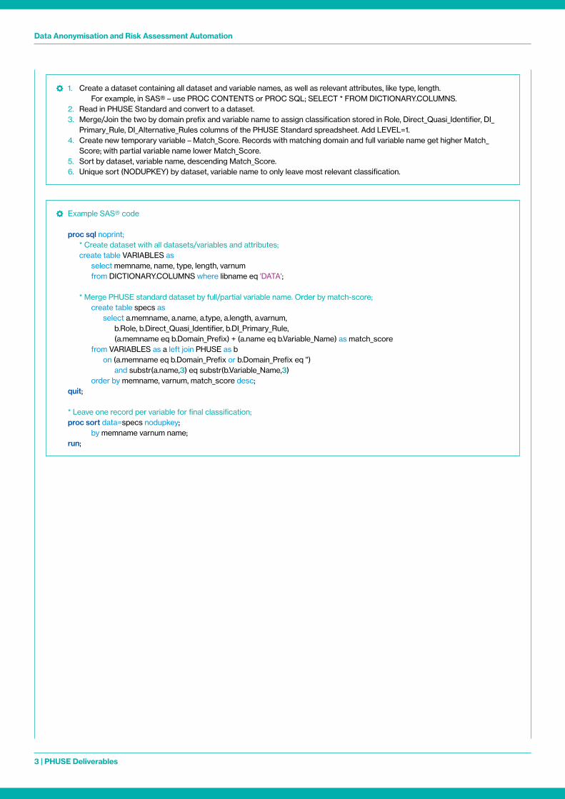
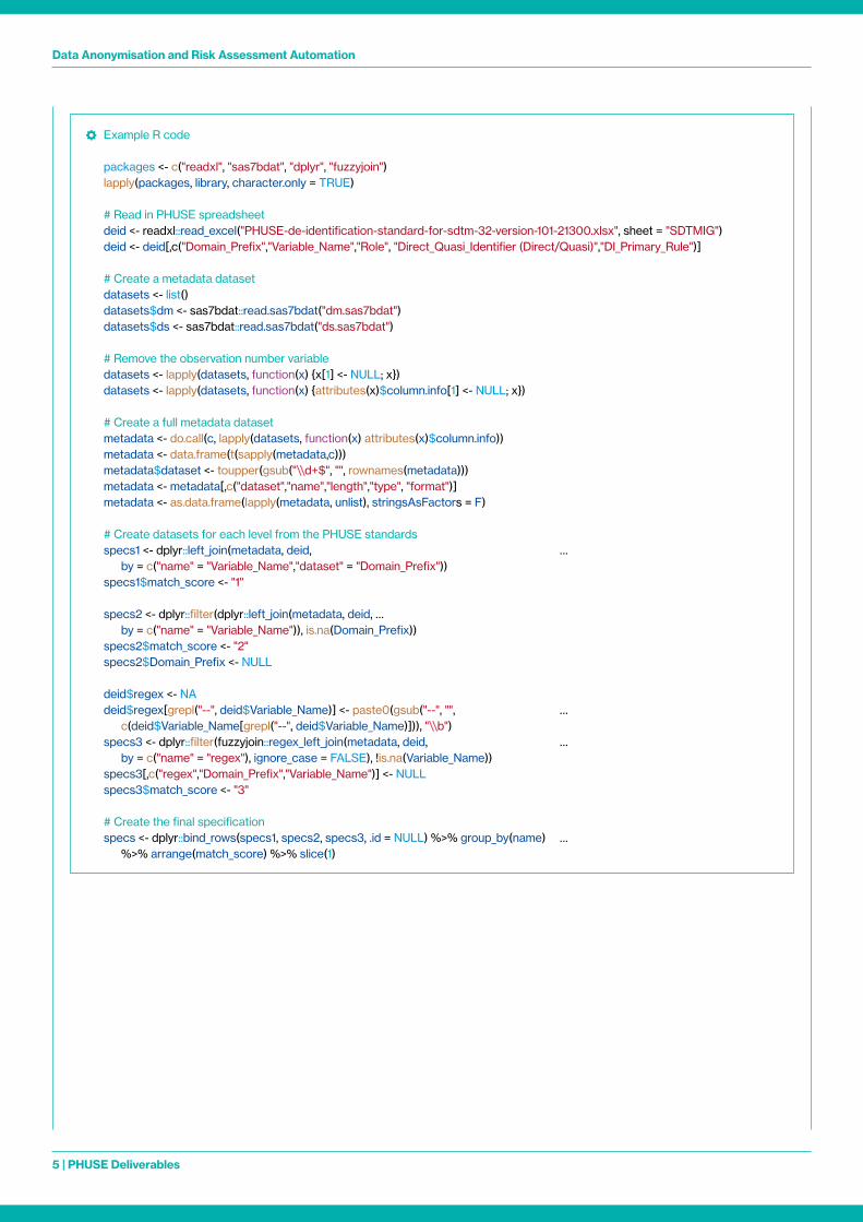
1 Create a dataset containing all dataset and variable names, as well as relevant attributes, like type, length For example, in SAS® – use PROC CONTENTS or PROC SQL; SELECT * FROM DICTIONARY COLUMNS 2 Read in PHUSE Standard and convert to a dataset 3 Merge/Join the two by domain prefix and variable name to assign classification stored in Role, Direct_Quasi_Identifier, DI_

Primary_Rule, DI_Alternative_Rules columns of the PHUSE Standard spreadsheet Add LEVEL=1 4 Create new temporary variable – Match_Score Records with matching domain and full variable name get higher Match_

Score; with partial variable name lower Match_Score 5 Sort by dataset, variable name, descending Match_Score 6 Unique sort (NODUPKEY) by dataset, variable name to only leave most relevant classification

Example SAS® code

proc sql noprint; * Create dataset with all datasets/variables and attributes; create table VARIABLES as select memname, name, type, length, varnum from DICTIONARY COLUMNS where libname eq 'DATA';

* Merge PHUSE standard dataset by full/partial variable name Order by match-score; create table specs as select a memname, a name, a type, a length, a varnum, b Role, b Direct_Quasi_Identifier, b DI_Primary_Rule, (a memname eq b Domain_Prefix) + (a name eq b Variable_Name) as match_score from VARIABLES as a left join PHUSE as b on (a memname eq b Domain_Prefix or b Domain_Prefix eq '') and substr(a name,3) eq substr(b Variable_Name,3) order by memname, varnum, match_score desc; quit;

* Leave one record per variable for final classification; proc sort data=specs nodupkey; by memname varnum name; run;



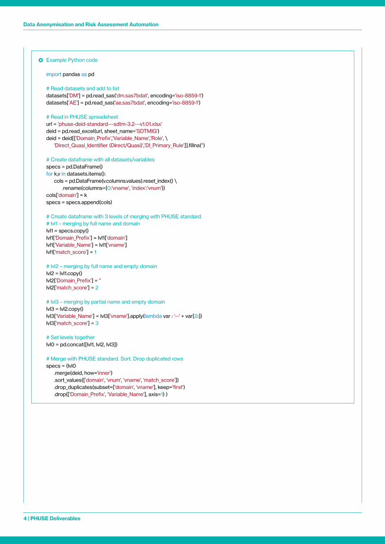
Example Python code

import pandas as pd

# Read datasets and add to list datasets['DM'] = pd read_sas('dm sas7bdat', encoding='iso-8859-1') datasets['AE'] = pd read_sas('ae sas7bdat', encoding='iso-8859-1')

# Read in PHUSE spreadsheet url = 'phuse-deid-standard---sdtm-3 2---v1 01 xlsx' deid = pd read_excel(url, sheet_name='SDTMIG') deid = deid[['Domain_Prefix','Variable_Name','Role', \ 'Direct_Quasi_Identifier (Direct/Quasi)','DI_Primary_Rule']] fillna('')

# Create dataframe with all datasets/variables specs = pd DataFrame() for k,v in datasets items(): cols = pd DataFrame(v columns values) reset_index() \ rename(columns={0:'vname', 'index':'vnum'}) cols['domain'] = k specs = specs append(cols)

# Create dataframe with 3 levels of merging with PHUSE standard # lvl1 – merging by full name and domain lvl1 = specs copy() lvl1['Domain_Prefix'] = lvl1['domain'] lvl1['Variable_Name'] = lvl1['vname'] lvl1['match_score'] = 1

# lvl2 – merging by full name and empty domain lvl2 = lvl1 copy() lvl2['Domain_Prefix'] = '' lvl2['match_score'] = 2

# lvl3 – merging by partial name and empty domain lvl3 = lvl2 copy() lvl3['Variable_Name'] = lvl3['vname'] apply(lambda var : '--' + var[2:]) lvl3['match_score'] = 3

# Set levels together lvl0 = pd concat([lvl1, lvl2, lvl3])

# Merge with PHUSE standard Sort Drop duplicated rows specs = (lvl0 merge(deid, how='inner') sort_values(['domain', 'vnum', 'vname', 'match_score']) drop_duplicates(subset=['domain', 'vname'], keep='first') drop(['Domain_Prefix', 'Variable_Name'], axis=1) )



Example R code

packages <- c("readxl", "sas7bdat", "dplyr", "fuzzyjoin") lapply(packages, library, character only = TRUE)

# Read in PHUSE spreadsheet deid <- readxl::read_excel("PHUSE-de-identification-standard-for-sdtm-32-version-101-21300 xlsx", sheet = "SDTMIG") deid <- deid[,c("Domain_Prefix","Variable_Name","Role", "Direct_Quasi_Identifier (Direct/Quasi)","DI_Primary_Rule")]

# Create a metadata dataset datasets <- list() datasets$dm <- sas7bdat::read sas7bdat("dm sas7bdat") datasets$ds <- sas7bdat::read sas7bdat("ds sas7bdat")

# Remove the observation number variable datasets <- lapply(datasets, function(x) {x[1] <- NULL; x}) datasets <- lapply(datasets, function(x) {attributes(x)$column info[1] <- NULL; x})

# Create a full metadata dataset metadata <- do call(c, lapply(datasets, function(x) attributes(x)$column info)) metadata <- data frame(t(sapply(metadata,c))) metadata$dataset <- toupper(gsub("\\d+$", "", rownames(metadata))) metadata <- metadata[,c("dataset","name","length","type", "format")] metadata <- as data frame(lapply(metadata, unlist), stringsAsFactors = F)

# Create datasets for each level from the PHUSE standards specs1 <- dplyr::left_join(metadata, deid, … by = c("name" = "Variable_Name","dataset" = "Domain_Prefix")) specs1$match_score <- "1"

specs2 <- dplyr::filter(dplyr::left_join(metadata, deid, … by = c("name" = "Variable_Name")), is na(Domain_Prefix)) specs2$match_score <- "2" specs2$Domain_Prefix <- NULL

deid$regex <- NA deid$regex[grepl("--", deid$Variable_Name)] <- paste0(gsub("--", "", … c(deid$Variable_Name[grepl("--", deid$Variable_Name)])), "\\b") specs3 <- dplyr::filter(fuzzyjoin::regex_left_join(metadata, deid, … by = c("name" = "regex"), ignore_case = FALSE), !is na(Variable_Name)) specs3[,c("regex","Domain_Prefix","Variable_Name")] <- NULL specs3$match_score <- "3"

# Create the final specification specs <- dplyr::bind_rows(specs1, specs2, specs3, id = NULL) %>% group_by(name) … %>% arrange(match_score) %>% slice(1)



3.2. Find identifiers by variable name and content

3.2.1. Subject IDs. Site, lab, test, reference IDs

Subject IDs are classified as direct identifiers They will be present in all subject level datasets and easy to find Some variables will contain only the subject ID (SUBJID), while others will combine it with study ID (USUBJID) In the case when multiple types of subject IDs are available it is advised to keep one and drop the others

When working with multiple studies, especially if extension studies are part of the package, it is possible that different USUBJID values refer to the same subject For example, “CT1/1001” in trial CT1 and “CT2/1001” in extension trial CT2 may refer to the same subject Those IDs should be dealt with in such a way that preserves the link between them

Other ID variables can also be found in datasets – SITEID, --REFID, --SPID, --SEQ, --GRPID, *ID They will need to be pseudonymised if they are needed in the planned analysis or dropped if they have no analytical value

3.2.3. Demographic and baseline characteristics

Demographic details are stored in DM or equivalent dataset: SEX, AGE, COUNTRY, RACE, ETHNIC

Body measurements can be found in VS (Vital Signs) or equivalent dataset

SDTM standard uses vertical structure: VS VSTESTCD = [“WEIGHT”, “HEIGHT”, “BMI”, etc ] Baseline values should be considered for identifier classification

Other data structures may store the values horizontally, in individual variables (WEIGHT, WGHT, HEIGHT, HGHT, etc ) Beyond using the baseline value as the quasi-identifier, it may be worth considering whether longitudinal changes in some parameters (e g weight) could aid re-identification efforts

3.2.4. Birth/death dates

Birth and death dates can be found in dedicated variables, e g BRTHDTC (Date/Time of Birth), DTHDTC (Date/Time of Death) However, those details can also be found in other variables, e g --OUT (Outcome of Event), as well as the AE (Adverse Events) and DS (Disposition) datasets

Birth dates should be removed from the datasets Death dates need to be offset

Some variables will contain information of death occurring, without revealing the actual date, e g DTHFL (Subject Death Flag), --SDTH (Results in Death), --DTHREL (Relationship to Death) Fatal events should be considered for further de-identification for low frequency of dead subjects

3.2.5. Verbatim terms and free-entry (comments) variables

Variables containing comments and other free-entry text (e g verbatim terms) can potentially contain information which can be used to infer values of quasi-identifiers This is especially true with regard to datasets CO (Comments) and FA (Findings About)

The primary rule for any variables which have their coded versions present (e g --TERM, when --DECOD, --BODSYS also exist in a dataset) is to drop the verbatim term variables and keep the coded ones

For variables where coded counterparts are not present and

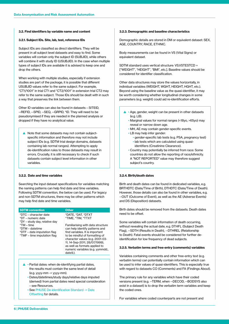
3.2.2. Date and time variables

Searching the input dataset specifications for variables matching the naming patterns can help find date and time variables Following SDTM convention, the below can be used For legacy and non-SDTM structures, there may be other patterns which may help find date and time variables

Note that some datasets may not contain subject-specific information and therefore may not include subject IDs (e g SDTM trial design domains, datasets containing lab normal ranges) Attempting to apply de-identification rules to those datasets may result in errors Crucially, it is still necessary to check if such datasets contain subject level information in other variables

SDTM convention Other

*DTC – character date *DT – numeric date*DY – study day, relative day*TM – time*DTM – datetime*DTF – date imputation flag*TMF – time imputation flag

*DATE, *DAT, *DTXT*TIME, *TIM, *TTXT

Familiarising with data structure can help identify patterns and find variables It is important to be mindful of formatting of character values (e g 2001-03-11, 14-Sep-2011, 28/07/1999), as well as formats applied to numeric variables (e g yymmdd , date9 )

• Partial dates: when de-identifying partial dates, the results must contain the same level of detail (e g yyyy-mm -> yyyy-mm)

• Dates/datetimes/study days/relative days imputed (derived) from partial dates need special consideration – see Resources

• See PHUSE De-identification Standard -> Date Offsetting for details

• Age, gender, weight can be present in other datasets (e g LB)

• Marginal values for normal ranges (<18yo, >65yo) may reveal or narrow down age

• MH, AE may contain gender-specific events • LB may help infer gender: • gender-specific lab tests (e g PSA, pregnancy test) • lab tests which are calculated using quasi-

identifiers (Creatinine Clearance) • Country may potentially be inferred from race: Some

countries do not allow the reporting of race/ethnicity A "NOT REPORTED" value may therefore suggest subject's country

https://www.phusewiki.org/docs/Data%20Transparency%20De-Identification/date-offsetting%20appendix-1--v200-19889.pdf




which are not relevant for the research, request the primary rule should also be to drop them

For uncoded variables which are required for the research request (needed for the planned analysis), the PHUSE standard suggests the “Review and Redact” approach Values of variables like --TERM (Reported Term) and CO COVAL (Comment) should be reviewed to check if they contain details like dates, names, places, local information, spelling If the variable cannot be dropped outright, all values should be thoroughly reviewed, and the details should be redacted within the text

3.2.6. Values (sex, age, race, dates, etc.) within result qualifier variables (--ORRES, --STRESC, --STRESN), SUPPQUAL datasets

Looking through test and characteristic names in --TEST (Name of Measurement, Test or Examination), --TESTCD (Short Name of Test or Examination) variables can reveal additional occurrences of information classified as personally identifying The values which may require de-identifying will be stored in result variables, i e --ORRES (Result or Finding in Original Units), --STRESC (Result or Finding in Standard Format), --STRESN (Numeric Result/Finding in Standard Units)

For SUPP* datasets, test and characteristic names are stored in QNAM and values are found in QVAL

3.2.7. Sensitive information (pregnancy, abortions, mental health, family, etc.)

Variables containing verbatim text (e g AE, CM, MH, CO, SUPP*) should be checked to find sensitive information, which may need to be redacted or removed The decision should be driven by the requirements of the request If such information is necessary for the planned analysis, it should be considered to be kept Otherwise, it can be deleted to reduce exposure in case of a data breach

Examples of terms to look for: pregn*, gestation*, prematur*, abort*, miscarria*, depres*, mental*, suicid*, mother*, father*, brother*, sister*, twin*, son*, daughter*

3.2.8. Rare diseases reported in Adverse Event & Medical History data

A standard AE frequency table may help identify AEs, MHs and CMs which are highly unique in the study population Those can be checked against registries to assess their uniqueness and need for anonymisation For example, a single case of

Consider dropping --ORRES variables if --STRESC/--STRESN is present

• Look for singular and plural forms and ignore case Use wildcards to look for parts of words Be aware of common misspellings and foreign language words

• Once identified, consider context, uniqueness and risk of re-identification versus data utility/quality

• Build a list of common terms for future use

the common cold in a study does not increase the risk of re-identification in general population

4. Define De-identification Rules, Build Specifications

Once all direct and quasi-identifiers have been found, the next step is to prepare dataset specifications by assigning de-identification rules to each variable across all datasets Based on the classification of all identifiers and non-identifiers each variable should be assigned a corresponding rule

4.1. Dataset-level rules

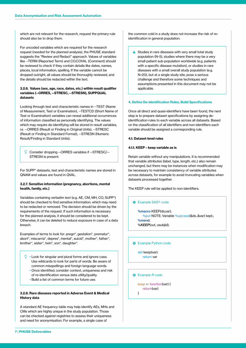
4.1.1. KEEP – keep variable as is

Retain variable without any manipulations It is recommended that variable attributes (label, type, length, etc ) also remain unchanged, but there may be instances when modification may be necessary to maintain consistency of variable attributes across datasets, for example to avoid truncating variables when datasets processed together

The KEEP rule will be applied to non-identifiers

Studies in rare diseases with very small total study population (N~5), studies where there may be a very small patient sub-population worldwide (e g patients with a specific disease mutation), or studies in rare diseases with a small overall study population (e g N<20), but at a single study site, pose a serious challenge and therefore some techniques and assumptions presented in this document may not be applicable

Example SAS® code

%macro KEEP(ds,var); %put NOTE: Variable %upcase(&ds &var) kept ; %mend; %KEEP(out, usubjid);

Example Python code

def keep(var): return var

Example R code

keep <- function(var) { return(var) }



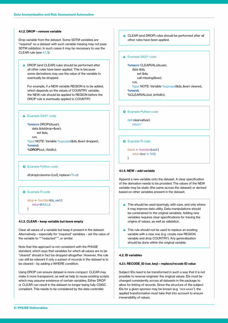
4.1.2. DROP – remove variable

Drop variable from the dataset Some SDTM variables are “required” so a dataset with such variable missing may not pass SDTM validation In such cases it may be necessary to use the CLEAR rule (see 4 1 3)

4.1.3. CLEAR – keep variable but leave empty

Clear all values of a variable but keep it present in the dataset Alternatively – especially for “required” variables – set the value of the variable to “**redacted**”, or similar

Note that this approach is not consistent with the PHUSE standard, which says that variables for which all values are to be “cleared” should in fact be dropped altogether However, this rule can still be relevant if only a subset of records in the dataset is to be cleared – by adding a WHERE condition

Using DROP can ensure dataset is more compact CLEAR may make it more transparent, as well as help to reuse existing scripts which may assume existence of certain variables Either DROP or CLEAR can result in the dataset no longer being fully CDISC compliant This needs to be considered by the data controller

4.1.4. NEW – add variable

Append a new variable onto the dataset A clear specification of the derivation needs to be provided The values of the NEW variable may be static (the same across the dataset) or derived based on other variables present in the dataset

4.2. ID variables

4.2.1. RECODE_ID (var, key) – replace/recode ID value

Subject IDs need to be transformed in such a way that it is not possible to reverse-engineer the original values IDs must be changed consistently across all datasets in the package to allow for linking of records Since the structure of the subject IDs for a given sponsor may be known (e g “xxx-xxxx”), the applied transformation must take that into account to ensure irreversibility of values

Example Python code

df drop(columns=[col], inplace=True)

Example Python code

def clearval(var): return ''

Example R code

drop <- function(ds, var) { return(NULL) }

Example R code

blank <- function(var) { return(var <- NA) }

DROP (and CLEAR) rules should be performed after all other rules have been applied This is because some derivations may use the value of the variable to eventually be dropped

For example, if a NEW variable REGION is to be added, which depends on the values of COUNTRY variable, the NEW rule should be applied to REGION before the DROP rule is eventually applied to COUNTRY

Example SAS® code

%macro DROP(ds,var); data &ds(drop=&var); set &ds; run; %put NOTE: Variable %upcase(&ds &var) dropped ; %mend; %DROP(out, rfstdtc);

Example SAS® code

%macro CLEARVAL(ds,var); data &ds; set &ds; call missing(&var); run; %put NOTE: Variable %upcase(&ds &var) cleared ; %mend; %CLEARVAL(out, brthdtc);

CLEAR (and DROP) rules should be performed after all other rules have been applied

This should be used sparingly, with care, and only where it may improve data utility Data manipulations should be constrained to the original variables Adding new variables requires clear specifications for tracing the origins of values, as well as validation

This rule should not be used to replace an existing variable with a new one (e g create new REGION variable and drop COUNTRY) Any generalisation should be done within the original variable



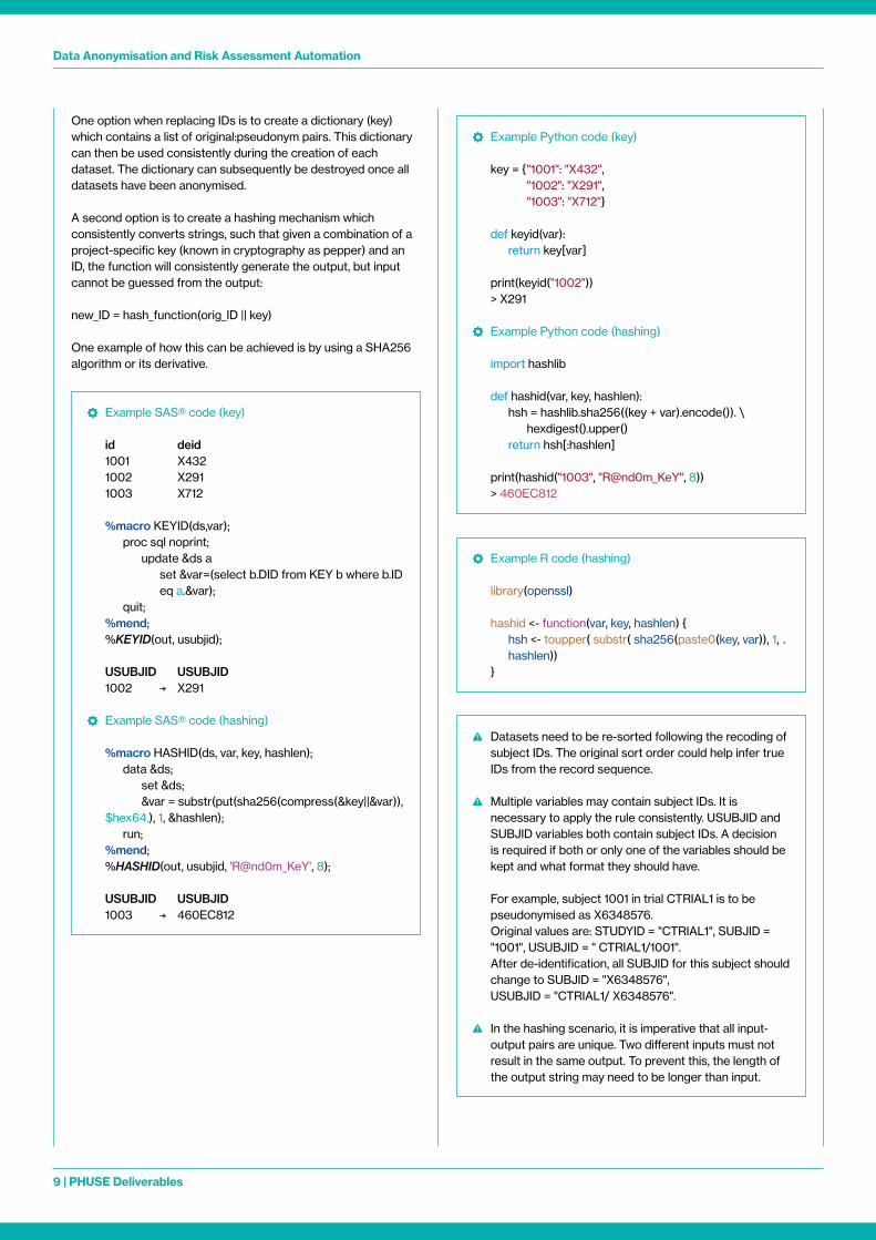
One option when replacing IDs is to create a dictionary (key) which contains a list of original:pseudonym pairs This dictionary can then be used consistently during the creation of each dataset The dictionary can subsequently be destroyed once all datasets have been anonymised

A second option is to create a hashing mechanism which consistently converts strings, such that given a combination of a project-specific key (known in cryptography as pepper) and an ID, the function will consistently generate the output, but input cannot be guessed from the output:

new_ID = hash_function(orig_ID || key)

One example of how this can be achieved is by using a SHA256 algorithm or its derivative

Example SAS® code (key)

id deid 1001 X432 1002 X291 1003 X712

%macro KEYID(ds,var); proc sql noprint; update &ds a set &var=(select b DID from KEY b where b ID

eq a &var); quit; %mend; %KEYID(out, usubjid);

USUBJID USUBJID 1002 → X291

Example SAS® code (hashing)

%macro HASHID(ds, var, key, hashlen); data &ds; set &ds; &var = substr(put(sha256(compress(&key||&var)), $hex64 ), 1, &hashlen); run; %mend; %HASHID(out, usubjid, 'R@nd0m_KeY', 8);

USUBJID USUBJID 1003 → 460EC812

Example Python code (key)

key = { "1001": "X432", "1002": "X291", "1003": "X712"}

def keyid(var): return key[var] print(keyid("1002")) > X291

Example Python code (hashing)

import hashlib

def hashid(var, key, hashlen): hsh = hashlib sha256((key + var) encode()) \ hexdigest() upper() return hsh[:hashlen]

print(hashid("1003", "R@nd0m_KeY", 8)) > 460EC812

Example R code (hashing)

library(openssl)

hashid <- function(var, key, hashlen) { hsh <- toupper( substr( sha256(paste0(key, var)), 1,

hashlen)) }

Datasets need to be re-sorted following the recoding of subject IDs The original sort order could help infer true IDs from the record sequence

Multiple variables may contain subject IDs It is necessary to apply the rule consistently USUBJID and SUBJID variables both contain subject IDs A decision is required if both or only one of the variables should be kept and what format they should have

For example, subject 1001 in trial CTRIAL1 is to be pseudonymised as X6348576

Original values are: STUDYID = "CTRIAL1", SUBJID = "1001", USUBJID = " CTRIAL1/1001"

After de-identification, all SUBJID for this subject should change to SUBJID = "X6348576",

USUBJID = "CTRIAL1/ X6348576"

In the hashing scenario, it is imperative that all input-output pairs are unique Two different inputs must not result in the same output To prevent this, the length of the output string may need to be longer than input



Some definitions of “anonymisation” include a clause that any existing key needs to be destroyed for the data to be “legally” considered anonymised To facilitate this, the key dataset/dictionary or key (pepper) used in hashing needs to be destroyed at the end of the anonymisation process

The OFFSET rule can include an optional parameter to only keep the year or year-month

For example, birth date can be offset and consequently truncated to only keep the birth year

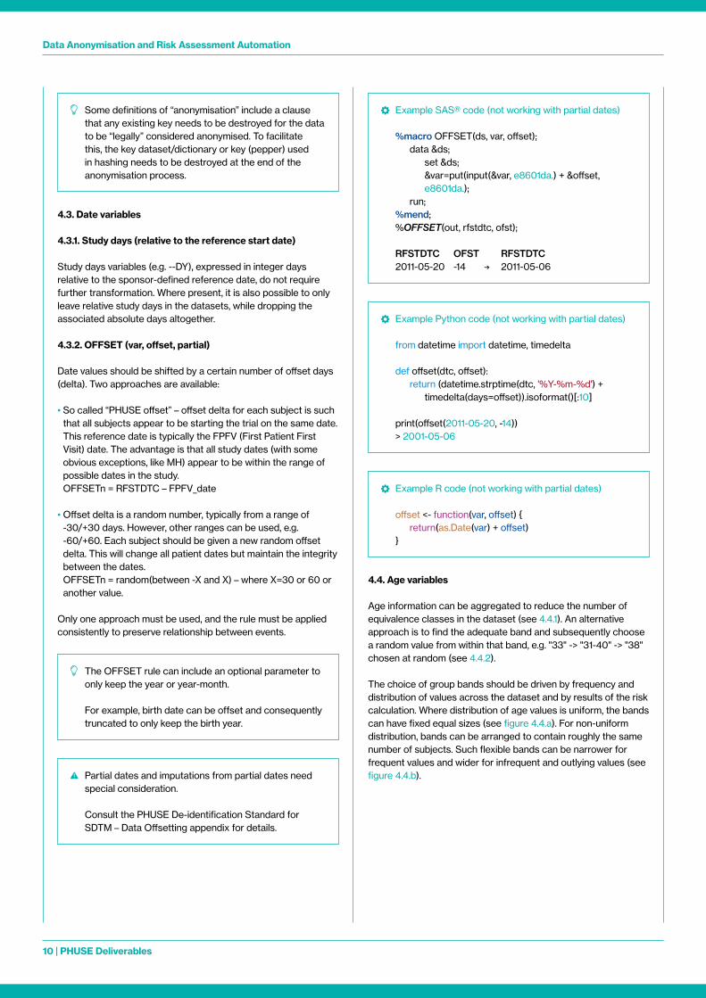
4.3. Date variables

4.3.1. Study days (relative to the reference start date)

Study days variables (e g --DY), expressed in integer days relative to the sponsor-defined reference date, do not require further transformation Where present, it is also possible to only leave relative study days in the datasets, while dropping the associated absolute days altogether

4.3.2. OFFSET (var, offset, partial)

Date values should be shifted by a certain number of offset days (delta) Two approaches are available:

• So called “PHUSE offset” – offset delta for each subject is such that all subjects appear to be starting the trial on the same date This reference date is typically the FPFV (First Patient First Visit) date The advantage is that all study dates (with some obvious exceptions, like MH) appear to be within the range of possible dates in the study OFFSETn = RFSTDTC – FPFV_date

• Offset delta is a random number, typically from a range of -30/+30 days However, other ranges can be used, e g -60/+60 Each subject should be given a new random offset delta This will change all patient dates but maintain the integrity between the dates OFFSETn = random(between -X and X) – where X=30 or 60 or another value

Only one approach must be used, and the rule must be applied consistently to preserve relationship between events

4.4. Age variables

Age information can be aggregated to reduce the number of equivalence classes in the dataset (see 4 4 1) An alternative approach is to find the adequate band and subsequently choose a random value from within that band, e g "33" -> "31-40" -> "38" chosen at random (see 4 4 2)

The choice of group bands should be driven by frequency and distribution of values across the dataset and by results of the risk calculation Where distribution of age values is uniform, the bands can have fixed equal sizes (see figure 4 4 a) For non-uniform distribution, bands can be arranged to contain roughly the same number of subjects Such flexible bands can be narrower for frequent values and wider for infrequent and outlying values (see figure 4 4 b) Partial dates and imputations from partial dates need

special consideration

Consult the PHUSE De-identification Standard for SDTM – Data Offsetting appendix for details

Example SAS® code (not working with partial dates)

%macro OFFSET(ds, var, offset); data &ds; set &ds; &var=put(input(&var, e8601da ) + &offset,

e8601da ); run; %mend; %OFFSET(out, rfstdtc, ofst);

RFSTDTC OFST RFSTDTC 2011-05-20 -14 → 2011-05-06

Example Python code (not working with partial dates)

from datetime import datetime, timedelta

def offset(dtc, offset): return (datetime strptime(dtc, '%Y-%m-%d') + timedelta(days=offset)) isoformat()[:10]

print(offset(2011-05-20, -14)) > 2001-05-06

Example R code (not working with partial dates)

offset <- function(var, offset) { return(as Date(var) + offset) }



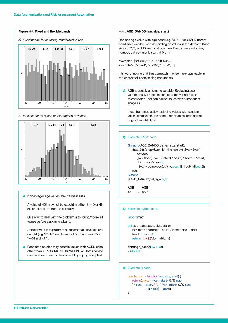
Figure 4.4. Fixed and flexible bands

a) Fixed bands for uniformly distributed values

b) Flexible bands based on distribution of values

Non-integer age values may cause issues A value of 40 1 may not be caught in either 31-40 or 41-

50 bracket if not treated carefully

One way to deal with the problem is to round/floor/ceil values before assigning a band

Another way is to program bands so that all values are caught (e g "31-40" can be in fact ">30 and <=40" or ">=31 and <41")

Paediatric studies may contain values with AGEU units other than YEARS MONTHS, WEEKS or DAYS can be used and may need to be unified if grouping is applied

AGE is usually a numeric variable Replacing age with bands will result in changing the variable type to character This can cause issues with subsequent analyses

It can be remedied by replacing values with random values from within the band This enables keeping the original variable type

4.4.1. AGE_BANDS (var, size, start)

Replace age value with age band (e g "33" -> "31-35") Different band sizes can be used depending on values in the dataset Band sizes of 2, 5, and 10 are most common Bands can start at any number, but commonly start at 0 or 1:

example 1 ["21-30", "31-40", "41-50", ]example 2 ["20-24", "25-29", "30-34", ]

It is worth noting that this approach may be more applicable in the context of anonymising documents

Example SAS® code

%macro AGE_BANDS(ds, var, size, start); data &ds(drop=&var _lo _hi rename=(_&var=&var)); set &ds; _lo = floor((&var - &start) / &size) * &size + &start; _hi = _lo + &size - 1; _&var = compress(put(_lo,best )||'-'||put(_hi,best )); run; %mend; %AGE_BANDS(out, age, 5, 1);

AGE AGE 47 → 46-50

Example Python code

import math

def age_bands(age, size, start): lo = math floor((age - start) / size) * size + start hi = lo + size - 1 return "({} - {})" format(lo, hi)

print(age_bands(47, 5, 0)) > (45-49)

Example R code

age_bands <- function(var, size, start) { return(paste((((var - start) %/% size ) * size) + start, "-", ((((var - start) %/% size) + 1) * size) + start)) }



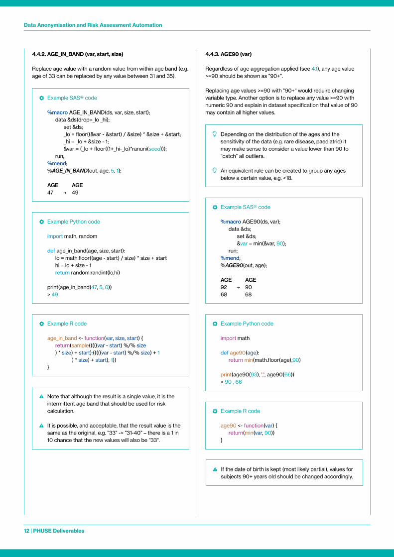
4.4.2. AGE_IN_BAND (var, start, size)

Replace age value with a random value from within age band (e g age of 33 can be replaced by any value between 31 and 35)

Example SAS® code

%macro AGE_IN_BAND(ds, var, size, start); data &ds(drop=_lo _hi); set &ds; _lo = floor((&var - &start) / &size) * &size + &start; _hi = _lo + &size - 1; &var = (_lo + floor((1+_hi-_lo)*ranuni(seed))); run; %mend; %AGE_IN_BAND(out, age, 5, 1);

AGE AGE 47 → 49

Example SAS® code

%macro AGE90(ds, var); data &ds; set &ds; &var = min(&var, 90); run; %mend; %AGE90(out, age);

AGE AGE 92 → 90 68 68

Example Python code

import math

def age90(age): return min(math floor(age),90)

print(age90(93), ',', age90(66)) > 90 , 66

Example R code

age90 <- function(var) { return(min(var, 90)) }

Example Python code

import math, random

def age_in_band(age, size, start): lo = math floor((age - start) / size) * size + start hi = lo + size - 1 return random randint(lo,hi)

print(age_in_band(47, 5, 0)) > 49

Example R code

age_in_band <- function(var, size, start) { return(sample(((((var - start) %/% size ) * size) + start):(((((var - start) %/% size) + 1 ) * size) + start), 1)) }

Note that although the result is a single value, it is the intermittent age band that should be used for risk calculation

It is possible, and acceptable, that the result value is the same as the original, e g "33" -> "31-40" – there is a 1 in 10 chance that the new values will also be "33"

If the date of birth is kept (most likely partial), values for subjects 90+ years old should be changed accordingly

4.4.3. AGE90 (var)

Regardless of age aggregation applied (see 4 1), any age value >=90 should be shown as "90+"

Replacing age values >=90 with "90+" would require changing variable type Another option is to replace any value >=90 with numeric 90 and explain in dataset specification that value of 90 may contain all higher values

Depending on the distribution of the ages and the sensitivity of the data (e g rare disease, paediatric) it may make sense to consider a value lower than 90 to “catch” all outliers

An equivalent rule can be created to group any ages below a certain value, e g <18



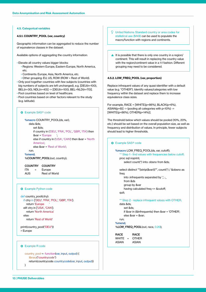
4.5. Categorical variables

4.5.1. COUNTRY_POOL (var, country)

Geographic information can be aggregated to reduce the number of equivalence classes in the dataset

Available options of aggregating the country information:

• Elevate all country values bigger blocks: • Regions: Western Europe, Eastern Europe, North America,

etc • Continents: Europe, Asia, North America, etc • Other grouping: EU, US, ROW (ROW = Rest of World) • Only pool together countries with few subjects (countries with

big numbers of subjects are left unchanged), e g [DEU(n=100), BEL(n=30), NDL(n=40)] -> [DEU(n=100), BEL+NLD(n=70)]

• Pool countries based on level of healthcare • Pool countries based on other factors relevant to the study

(e g latitude)

4.5.2. LOW_FREQ_POOL (var, proportion)

Replace infrequent values of any quasi-identifier with a default value (e g "OTHER") Identify values/categories with low frequency within the dataset and replace them to increase equivalence class sizes

For example, RACE = [WHITE(p=86%), BLACK(p=6%), ASIAN(p=8)] -> (pooling all categories with p<10%) -> [WHITE(p=86%), OTHER(p=14%)]

The threshold below which values should be pooled (10%, 20%, etc ) should be set based on the overall population size, as well as frequency and distribution of values In principle, fewer subjects should lead to higher thresholds

Example SAS® code

%macro COUNTRY_POOL(ds, var); data &ds; set &ds; if country in ('DEU', 'FRA', 'POL', 'GBR', 'ITA') then

&var = 'Europe '; else if country in ('USA', 'CAN') then &var = 'North

America'; else &var = 'Rest of World'; run; %mend; %COUNTRY_POOL(out, country);

COUNTRY COUNTRY ITA → Europe AUS Rest of World

Example SAS® code

%macro LOW_FREQ_POOL(ds, var, cutoff); ** Step 1 - find values with frequencies below cutoff; proc sql noprint; select count(*) into: obsno from &ds;

select distinct '"'||strip(&var)||'"', count(*) / &obsno as freq

into :infrequents separated by ',', :_ from &ds group by &var having calculated freq <= &cutoff; quit; ** Step 2 - replace infrequent values with OTHER; data &ds; set &ds; if &var in (&infrequents) then &var = 'OTHER'; else &var = &var; run; %mend; %LOW_FREQ_POOL(out, race, 0 20);

RACE RACE WHITE → OTHER ASIAN ASIAN

Example Python code

def country_pool(ctry): if ctry in ['DEU', 'FRA', 'POL', 'GBR', 'ITA']: return 'Europe ' elif ctry in ['USA', 'CAN']: return 'North America' else: return 'Rest of World'

print(country_pool("DEU"))> Europe

Example R code

country_pool <- function(var, input, output) { library("countrycode") return(countrycode::countrycode(var, input, output)) }

United Nations: Standard country or area codes for statistical use (M49) can be used to populate the macro/function with regions and continents

It is possible that there is only one country in a region/continent This will result in replacing the country value with the region/continent value in a 1:1 fashion Different grouping may need to be considered

https://unstats.un.org/unsd/methodology/m49/overview/




Example Python code

import pandas as pd ## 1 Find values with frequency <= cutoff def find_low_freqs(df, var, cutoff): freqs = df[var] value_counts() / df shape[0] return freqs[freqs <= cutoff] index tolist()

infrequents = find_low_freqs(dm, 'RACE', 0 2) print(infrequents) > ['WHITE', 'ASIAN']

## 2 Apply rule with the list from (1) def low_freq_pool(var, low_freq_vals): if var in low_freq_vals: return 'OTHER' return var

print(low_freq_pool('WHITE', infrequents)) > OTHER print(low_freq_pool('BLACK OR AFRICAN AMERICAN', infrequents)) > BLACK OR AFRICAN AMERICAN

Example R code

low_freq_pool <- function(ds, var, cutoff) { freqs <- as data frame(table(ds[, c(var)])) freqs[, 2] <- freqs[, 2] / length(ds[, c(var)]) low_freqs <- as character(freqs[, 1][which(freqs[, 2] <

cutoff)]) ds[ds$RACE %in% low_freqs, ][, var] <- "OTHER" return(ds) }

Example SAS® code

%macro REDACT(ds, var, regex_pattern); data &ds; set &ds; &var = prxchange('s/'||&regex_pattern||'/**redacted**/i', -1, &var);; run; %mend; %REDACT(out, txt, '(\d+\ ?\d*)|(one)');

TXT TXT ONE Two 33 33 foUR, → **redacted** Two **redacted** foUR, 55 sIx 7 EiGhT **redacted** sIx **redacted** EiGhT

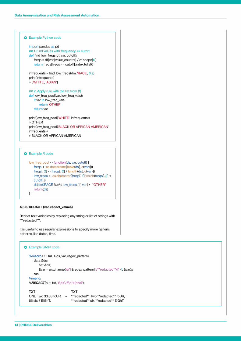
4.5.3. REDACT (var, redact_values)

Redact text variables by replacing any string or list of strings with "**redacted**"

It is useful to use regular expressions to specify more generic patterns, like dates, time



Example Python code

import re

def redact_regex(var, redact_values): for redaction in redact_values: print(redaction) regex = re compile(redaction, re IGNORECASE) var = re sub(regex, '**redacted**', var) return var

print(redact_regex("ONE Two 33 33 foUR 55 sIx ",['one', r'\d+\ ?\d*']))

> **redacted** Two **redacted** foUR **redacted** sIx

Example R code

redact <- function(var, redact_values) { return( gsub( pattern = redact_values, x = var, ignore case = TRUE, replacement = "**redacted**" ) ) }

4.6. Vertical datasets

All 4 2 – 4 5 rules can also be applied to vertical datasets In this case rules are applied conditionally (using a WHERE statement) to values of --ORRES/--STRESC/--STRESN/AVALC/AVAL based on --TESTCD/--TEST/PARAMCD/PARAM values More than one rule can be applied to the same variable within a dataset, using different WHERE conditions to transform values of different tests or characteristics

The same is true for Supplemental Qualifiers SDTM datasets

5.1.2. Inadvertent re-identification (recognition)

An inadvertent re-identification occurs when the recipient of the data recognises someone in the dataset The risk of such scenario is equivalent to the probability of the data recipient knowing a subject within the dataset well enough to identify them based on the information available

A method often used to estimate the probability of recognising a person in a dataset is expressed as:

where “150” is the average number of stable relationships a person can comfortably maintain – also known as the Dunbar number The value of 150 is suggested by literature discussing the risk or re-identification; however, other values (typically between 100 and 250) have also been proposed and can be considered

To factor in the location of the data recipient, it may be relevant to calculate Pr(inadvertent re-id) separately for each country and to choose the maximum of all countries

5. Calculate Residual Risk of Re-identification

The risk of re-identification is a product of two factors: the risk of a re-identification attempt being made, and the risk of successful re-identification if an attempt has indeed taken place

The former is linked to the context of disclosure (relationship with the recipient, contractual limitations, access restrictions, etc ) It is estimated once, at the beginning of the anonymisation process, and remains unchanged throughout The latter is based on the data itself and can be controlled and altered by applying different de-identification rules

5.1. Risk of re-identification attempt being made

5.1.1. Deliberate attack

In a deliberate attempt an attacker targets either a specific subject or any subject in the dataset Its probability will be a function of controls over the use of data, as well as the means and the motivation of the potential attacker

If the data controller has an established relationship with the data recipient, it is unlikely that an attack will be attempted as it would severely impact the relationship When data is shared with a researcher unknown to the data controller then reputation may be considered

Data shared through a secure portal, with access restrictions and restrictions on moving data in and out of the system, greatly reduces the risk Releasing the actual data using secure file transfer tools, email or thumb drive limits the level of control on who will use the data

Finally, the sensitivity of the data shared and the potential harm in an event of re-identification needs to be carefully considered when selecting the threshold

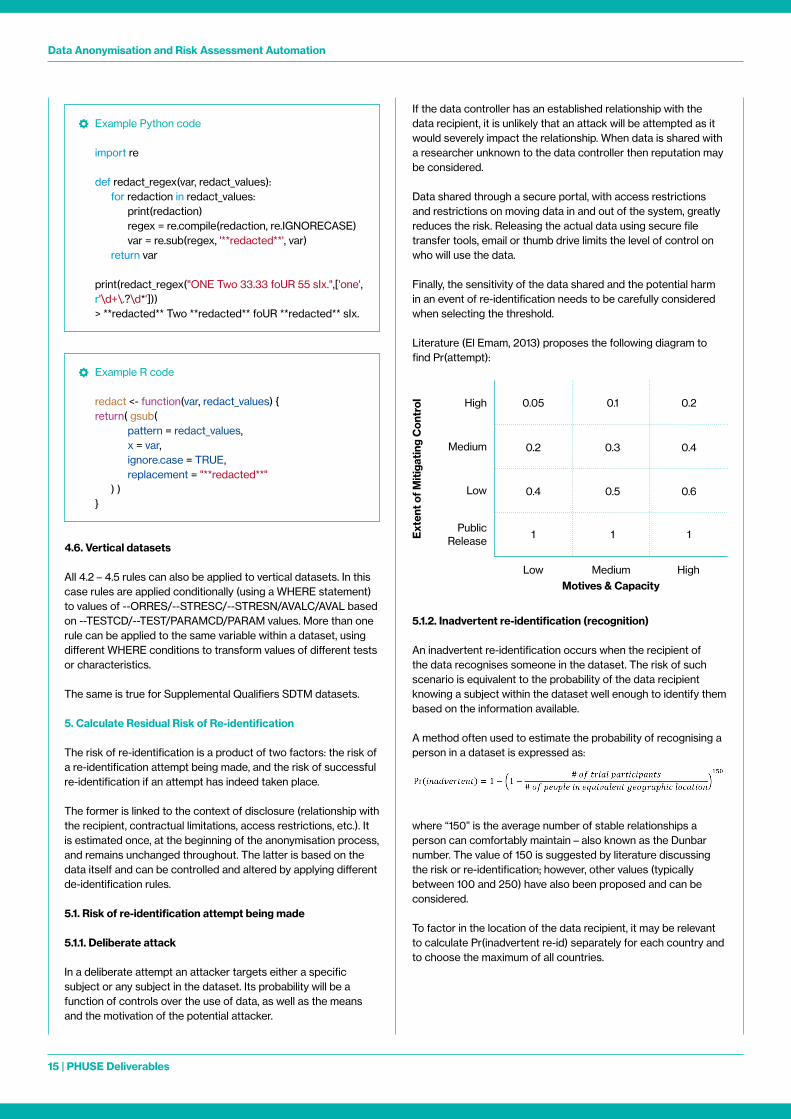
Literature (El Emam, 2013) proposes the following diagram to find Pr(attempt):

High 0 05 0 1 0 2

0 2 0 3 0 4

0 4 0 5 0 6

1 1 1

Medium

Low

PublicRelease

Low MediumMotives & Capacity

Ext

ent o

f Miti

gatin

g C

ontr

ol

High



The example study below has 2,500 participants in three countries – Denmark, France and Poland See the table below for number of participants, country populations and risk results

To calculate the risk for all countries together:

5.2. Selecting quasi-identifiers for calculating the risk of success

Age, sex, country (and other geographic details), race, and ethnicity are classified as quasi-identifiers and should be taken into the re-identification risk calculation

BMI is derived from a subject’s height and weight, so these should be considered as quasi-identifiers, too, especially the extreme values Height is generally (outside of paediatric studies) a fixed value and so can be derived if weight and BMI are present in the dataset Height is the easiest of those to observe with accuracy without technical apparatus Some data controllers choose to only keep BMI and drop height and weight as means of obscuring specific measurements

While the above variables are the typical candidates, the data controller should consider the full set of quasi-identifiers to add to the risk model for each given study

5.3. Base Dataset for calculating risk

All quasi-identifiers which should be used for re-identification risk calculation should be collated in a dataset which will contain:

• one record per subject,• one variable with a unique subject identifier (e g USUBJID),• separate variables for each quasi-identifier used in the

calculations – those should contain the original values, as found in the input dataset (de-identification rules will be applied later to find the optimal rule set – see 6 5)

This dataset will be referred to as Base Dataset, going forward

5.4. Risk of successful re-identification (assuming attempt has taken place)

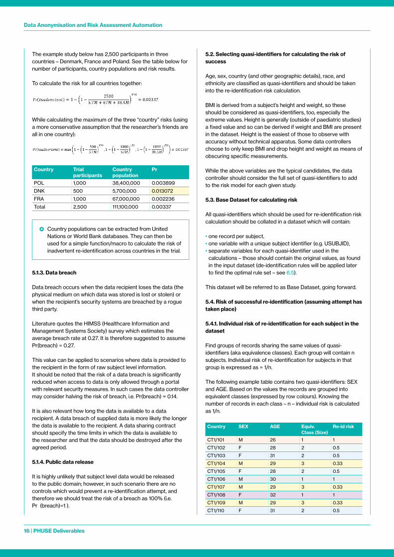
5.4.1. Individual risk of re-identification for each subject in the dataset

Find groups of records sharing the same values of quasi-identifiers (aka equivalence classes) Each group will contain n subjects Individual risk of re-identification for subjects in that group is expressed as = 1/n

The following example table contains two quasi-identifiers: SEX and AGE Based on the values the records are grouped into equivalent classes (expressed by row colours) Knowing the number of records in each class – n – individual risk is calculated as 1/n

While calculating the maximum of the three “country” risks (using a more conservative assumption that the researcher’s friends are all in one country):

5.1.3. Data breach

Data breach occurs when the data recipient loses the data (the physical medium on which data was stored is lost or stolen) or when the recipient’s security systems are breached by a rogue third party

Literature quotes the HIMSS (Healthcare Information and Management Systems Society) survey which estimates the average breach rate at 0 27 It is therefore suggested to assume Pr(breach) = 0 27

This value can be applied to scenarios where data is provided to the recipient in the form of raw subject level information It should be noted that the risk of a data breach is significantly reduced when access to data is only allowed through a portal with relevant security measures In such cases the data controller may consider halving the risk of breach, i e Pr(breach) = 0 14

It is also relevant how long the data is available to a data recipient A data breach of supplied data is more likely the longer the data is available to the recipient A data sharing contract should specify the time limits in which the data is available to the researcher and that the data should be destroyed after the agreed period

5.1.4. Public data release

It is highly unlikely that subject level data would be released to the public domain; however, in such scenario there are no controls which would prevent a re-identification attempt, and therefore we should treat the risk of a breach as 100% (i e Pr(breach)=1 )

Country Trial participants

Country population

Pr

POL 1,000 38,400,000 0 003899

DNK 500 5,700,000 0 013072

FRA 1,000 67,000,000 0 002236

Total 2,500 111,100,000 0 00337

Country SEX AGE Equiv. Class (Size)

Re-id risk

CT1/101 M 26 1 1

CT1/102 F 28 2 0 5

CT1/103 F 31 2 0 5

CT1/104 M 29 3 0 33

CT1/105 F 28 2 0 5

CT1/106 M 30 1 1

CT1/107 M 29 3 0 33

CT1/108 F 32 1 1

CT1/109 M 29 3 0 33

CT1/110 F 31 2 0 5

Country populations can be extracted from United Nations or World Bank databases They can then be used for a simple function/macro to calculate the risk of inadvertent re-identification across countries in the trial



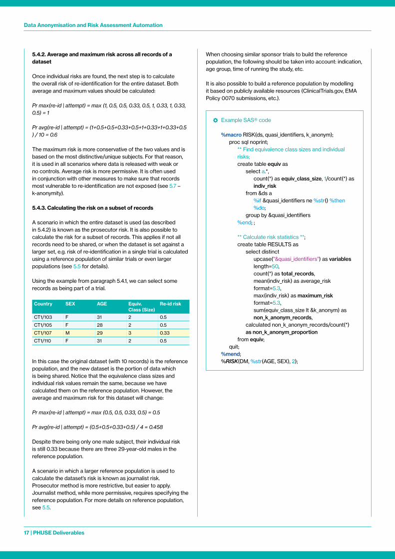
5.4.2. Average and maximum risk across all records of a dataset

Once individual risks are found, the next step is to calculate the overall risk of re-identification for the entire dataset Both average and maximum values should be calculated:

Pr max(re-id | attempt) = max (1, 0.5, 0.5, 0.33, 0.5, 1, 0.33, 1, 0.33, 0.5) = 1

Pr avg(re-id | attempt) = (1+0.5+0.5+0.33+0.5+1+0.33+1+0.33+0.5) / 10 = 0.6

The maximum risk is more conservative of the two values and is based on the most distinctive/unique subjects For that reason, it is used in all scenarios where data is released with weak or no controls Average risk is more permissive It is often used in conjunction with other measures to make sure that records most vulnerable to re-identification are not exposed (see 5 7 – k-anonymity)

5.4.3. Calculating the risk on a subset of records

A scenario in which the entire dataset is used (as described in 5 4 2) is known as the prosecutor risk It is also possible to calculate the risk for a subset of records This applies if not all records need to be shared, or when the dataset is set against a larger set, e g risk of re-identification in a single trial is calculated using a reference population of similar trials or even larger populations (see 5 5 for details)

Using the example from paragraph 5 4 1, we can select some records as being part of a trial

In this case the original dataset (with 10 records) is the reference population, and the new dataset is the portion of data which is being shared Notice that the equivalence class sizes and individual risk values remain the same, because we have calculated them on the reference population However, the average and maximum risk for this dataset will change:

Pr max(re-id | attempt) = max (0.5, 0.5, 0.33, 0.5) = 0.5

Pr avg(re-id | attempt) = (0.5+0.5+0.33+0.5) / 4 = 0.458

Despite there being only one male subject, their individual risk is still 0 33 because there are three 29-year-old males in the reference population

A scenario in which a larger reference population is used to calculate the dataset’s risk is known as journalist risk Prosecutor method is more restrictive, but easier to apply Journalist method, while more permissive, requires specifying the reference population For more details on reference population, see 5 5

Country SEX AGE Equiv. Class (Size)

Re-id risk

CT1/103 F 31 2 0 5

CT1/105 F 28 2 0 5

CT1/107 M 29 3 0 33

CT1/110 F 31 2 0 5

When choosing similar sponsor trials to build the reference population, the following should be taken into account: indication, age group, time of running the study, etc

It is also possible to build a reference population by modelling it based on publicly available resources (ClinicalTrials gov, EMA Policy 0070 submissions, etc )

Example SAS® code

%macro RISK(ds, quasi_identifiers, k_anonym); proc sql noprint; ** Find equivalence class sizes and individual

risks; create table equiv as select a *, count(*) as equiv_class_size, 1/count(*) as

indiv_risk from &ds a %if &quasi_identifiers ne %str() %then

%do; group by &quasi_identifiers %end; ; ** Calculate risk statistics **; create table RESULTS as select distinct upcase("&quasi_identifiers") as variables

length=50, count(*) as total_records, mean(indiv_risk) as average_risk

format=5 3, max(indiv_risk) as maximum_risk

format=5 3, sum(equiv_class_size lt &k_anonym) as

non_k_anonym_records, calculated non_k_anonym_records/count(*)

as non_k_anonym_proportion from equiv; quit; %mend; %RISK(DM, %str(AGE, SEX), 2);



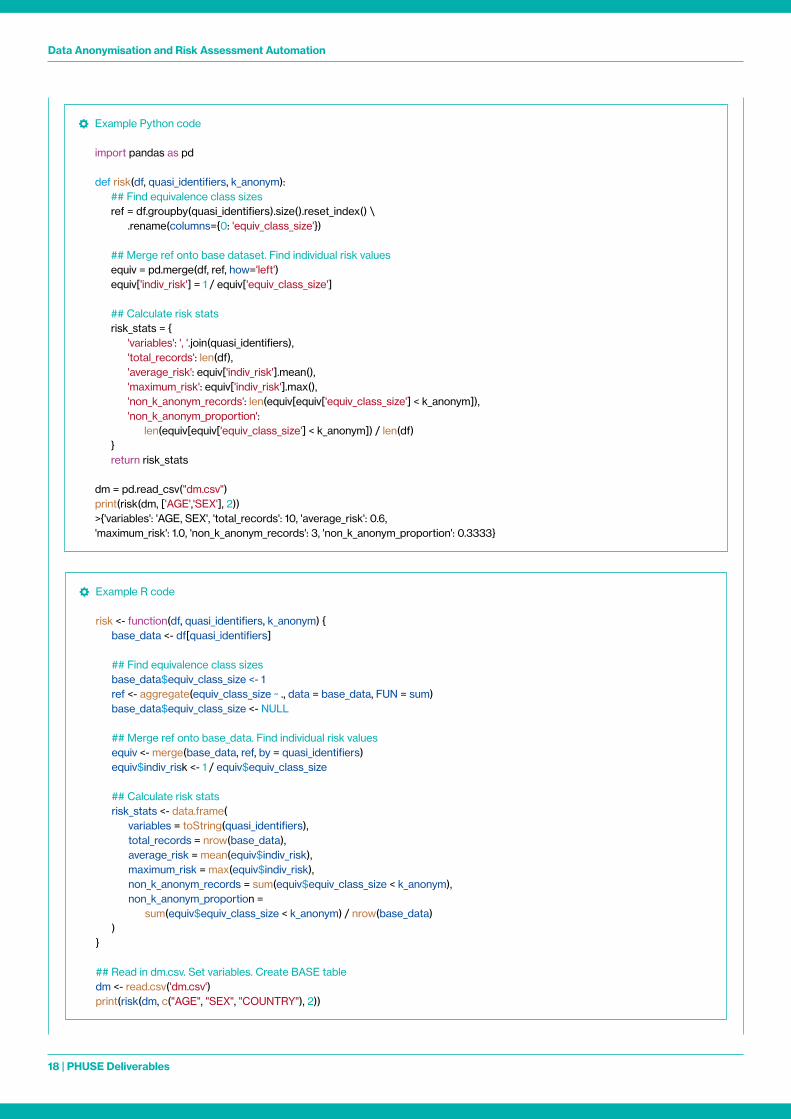
Example Python code

import pandas as pd

def risk(df, quasi_identifiers, k_anonym): ## Find equivalence class sizes ref = df groupby(quasi_identifiers) size() reset_index() \ rename(columns={0: 'equiv_class_size'})

## Merge ref onto base dataset Find individual risk values equiv = pd merge(df, ref, how='left') equiv['indiv_risk'] = 1 / equiv['equiv_class_size']

## Calculate risk stats risk_stats = { 'variables': ', ' join(quasi_identifiers), 'total_records': len(df), 'average_risk': equiv['indiv_risk'] mean(), 'maximum_risk': equiv['indiv_risk'] max(), 'non_k_anonym_records': len(equiv[equiv['equiv_class_size'] < k_anonym]), 'non_k_anonym_proportion': len(equiv[equiv['equiv_class_size'] < k_anonym]) / len(df) } return risk_stats

dm = pd read_csv("dm csv") print(risk(dm, ['AGE','SEX'], 2)) >{'variables': 'AGE, SEX', 'total_records': 10, 'average_risk': 0 6, 'maximum_risk': 1 0, 'non_k_anonym_records': 3, 'non_k_anonym_proportion': 0 3333}

Example R code

risk <- function(df, quasi_identifiers, k_anonym) { base_data <- df[quasi_identifiers] ## Find equivalence class sizes base_data$equiv_class_size <- 1 ref <- aggregate(equiv_class_size ~ , data = base_data, FUN = sum) base_data$equiv_class_size <- NULL ## Merge ref onto base_data Find individual risk values equiv <- merge(base_data, ref, by = quasi_identifiers) equiv$indiv_risk <- 1 / equiv$equiv_class_size ## Calculate risk stats risk_stats <- data frame( variables = toString(quasi_identifiers), total_records = nrow(base_data), average_risk = mean(equiv$indiv_risk), maximum_risk = max(equiv$indiv_risk), non_k_anonym_records = sum(equiv$equiv_class_size < k_anonym), non_k_anonym_proportion = sum(equiv$equiv_class_size < k_anonym) / nrow(base_data) ) }

## Read in dm csv Set variables Create BASE table dm <- read csv('dm csv') print(risk(dm, c("AGE", "SEX", "COUNTRY"), 2))



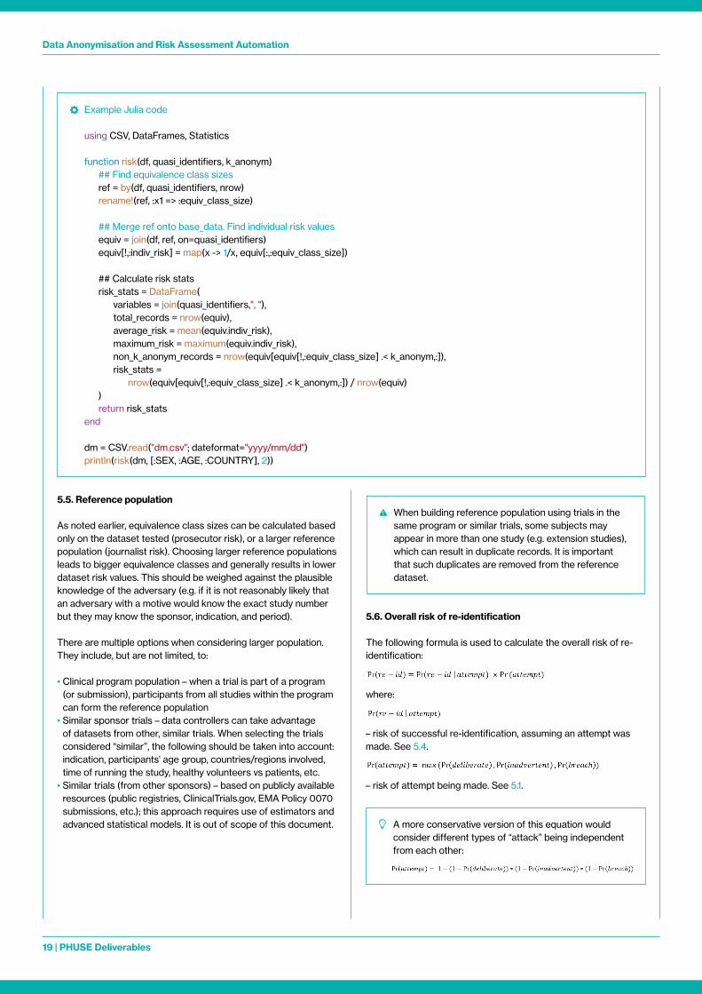
Example Julia code

using CSV, DataFrames, Statistics

function risk(df, quasi_identifiers, k_anonym) ## Find equivalence class sizes ref = by(df, quasi_identifiers, nrow) rename!(ref, :x1 => :equiv_class_size)

## Merge ref onto base_data Find individual risk values equiv = join(df, ref, on=quasi_identifiers) equiv[!,:indiv_risk] = map(x -> 1/x, equiv[:,:equiv_class_size])

## Calculate risk stats risk_stats = DataFrame( variables = join(quasi_identifiers,", "), total_records = nrow(equiv), average_risk = mean(equiv indiv_risk), maximum_risk = maximum(equiv indiv_risk), non_k_anonym_records = nrow(equiv[equiv[!,:equiv_class_size] < k_anonym,:]), risk_stats = nrow(equiv[equiv[!,:equiv_class_size] < k_anonym,:]) / nrow(equiv) ) return risk_stats end

dm = CSV read("dm csv"; dateformat="yyyy/mm/dd") println(risk(dm, [:SEX, :AGE, :COUNTRY], 2))

5.5. Reference population

As noted earlier, equivalence class sizes can be calculated based only on the dataset tested (prosecutor risk), or a larger reference population (journalist risk) Choosing larger reference populations leads to bigger equivalence classes and generally results in lower dataset risk values This should be weighed against the plausible knowledge of the adversary (e g if it is not reasonably likely that an adversary with a motive would know the exact study number but they may know the sponsor, indication, and period)

There are multiple options when considering larger population They include, but are not limited, to:

• Clinical program population – when a trial is part of a program (or submission), participants from all studies within the program can form the reference population

• Similar sponsor trials – data controllers can take advantage of datasets from other, similar trials When selecting the trials considered “similar”, the following should be taken into account: indication, participants’ age group, countries/regions involved, time of running the study, healthy volunteers vs patients, etc

• Similar trials (from other sponsors) – based on publicly available resources (public registries, ClinicalTrials gov, EMA Policy 0070 submissions, etc ); this approach requires use of estimators and advanced statistical models It is out of scope of this document

5.6. Overall risk of re-identification

The following formula is used to calculate the overall risk of re-identification:

where:

– risk of successful re-identification, assuming an attempt was made See 5 4

– risk of attempt being made See 5 1

When building reference population using trials in the same program or similar trials, some subjects may appear in more than one study (e g extension studies), which can result in duplicate records It is important that such duplicates are removed from the reference dataset

A more conservative version of this equation would consider different types of “attack” being independent from each other:



5.7. k-anonymity and uniqueness

Although the value of the average risk may be low enough to meet the threshold, on its own it might not be enough to deem the data safe for sharing One additional metric to utilise is k-anonymity, where k is the smallest equivalence class allowed to be left in the shared dataset For 2-anonymity, this means that there are at least two records that share any combination of values of quasi-identifiers (in other words, all equivalence class sizes are 2 or more); for 5-anonymity, at least five records (or equivalence classes not smaller than 5), etc

One way to implement this metric is to make sure that after all de-identification techniques have been applied, the k-anonymity condition is also met This way not only is the average risk acceptable but also no less than k records share the same characteristics in the dataset

A less strict approach is to calculate the percentage of records not meeting the k-anonymity criterion Under certain conditions, instead of anonymising the dataset to the point where k-anonymity is achieved across all records, it may be permissible to allow a small number of records (for example, <1%) to remain unique (< k similar records in dataset) Calculating the proportion of unique records can also aid in the iterative process of anonymisation as it can show how close to meeting all criteria the data is and identify equivalence classes which need to be taken care of

For sensitive data for public and controlled release, special consideration is required when selecting the threshold The threshold is a function of the impact of a successful re-identification and a factor of the sensitivity of the data and possible invasion of privacy

5.8. Threshold

5.8.1. Risk threshold

A threshold which is often used in the context of clinical trials and which offers a good balance between risk of data re-identification and data usability is a conservative value of 0 09 (or 9%) The same value is suggested as the preferred threshold for the EMA Policy 0070 submission and is often used by the clinical trials world It is possible to set a different threshold; however, this requires careful consideration of the sensitivity of the data and possible invasion of privacy, and clear justification

The optimal scenario is one in which the residual risk is just below the threshold as it would in general maximise data utility Besides, the residual risk for different transformation rules can be combined with measures of data utility (out of scope for this document) to find the most optimised set of rules that meets privacy objectives

5.8.2. “Uniqueness” threshold

It is possible that the average risk is below a desired threshold, but there are still unique records present in the dataset It is therefore prudent to check if k-anonymity condition has been met, independent of the risk value calculation, and – where relevant – find the proportion of non-k-anonymous records If k-anonymity is to be achieved across the entire dataset, the proportion of non-k-anonymous must be 0 In some cases, it may be acceptable to allow a small number of records not meeting the criterion, e g proportion of non-k-anonymous records <=1%, <=5%

The combination of average risk and k-anonymity check is known as “strict average”

6. Apply De-identification Rules to Dataset

6.1. The first scenario

So far, we have calculated the risk of re-identification for the Base Dataset (see 5 3) We should now test different options by applying de-identification rules to those quasi-identifiers The first step is to create a Rule Dataset This will have similar structure to the Base Dataset except each row will correspond to a scenario to test The base scenario assumes all quasi-identifiers to be kept and unchanged (KEEP rule assigned to each variables) An example Rule Dataset for this scenario could look as shown below:

Missing quasi-identifiers and too small values of k can both negatively impact privacy

k-anonymity is also weak against deterministic inference attacks, where sensitive information can be used to reidentify someone due to low diversity in an equivalence class

k-anonymity is subjective and so different releases of datasets could contain different information while satisfying k-anonymity This can lead to unwanted data attacks, the most basic being an unsorted data attack, where the k-anonymity data releases are performed differently but the sorted data structure is preserved (if reassigning patient numbers, this should not (!) happen) Two simultaneous distinct k-anonymity releases could allow a variable not previously determined to be a quasi-identifier to become a surrogate quasi-identifier and allow the k-anonymity to be broken and make the datasets more vulnerable Similarly, if the data changes over time (corrections, appended), then this could change the k-anonymity approach and could make the datasets more vulnerable if the attacker has access to historic datasets

AGE Sex Race Country

Keep Keep Keep Keep

6.2. Apply the de-identification rules

To apply rules to the Base Dataset, the steps below need to be followed:

• Read in a row from Rule Dataset • Iterate over variables in Rule Dataset to find Var:Rule pairs • Apply the corresponding rule to each variable of the Base

Dataset • Store the result as Transformed Dataset



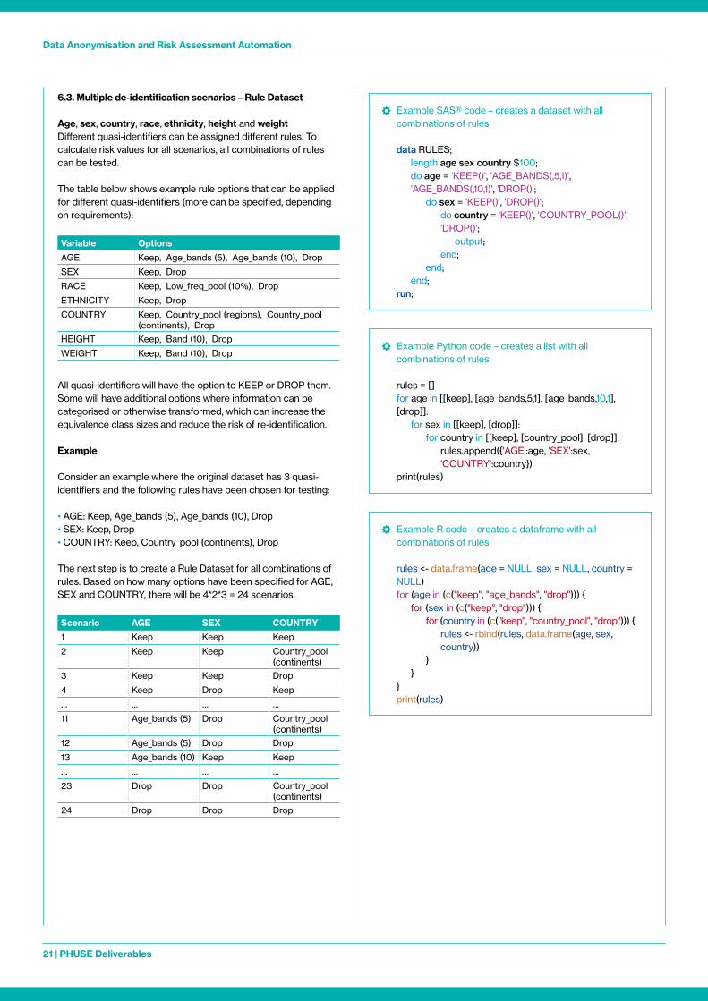
6.3. Multiple de-identification scenarios – Rule Dataset

Age, sex, country, race, ethnicity, height and weightDifferent quasi-identifiers can be assigned different rules To calculate risk values for all scenarios, all combinations of rules can be tested

The table below shows example rule options that can be applied for different quasi-identifiers (more can be specified, depending on requirements):

All quasi-identifiers will have the option to KEEP or DROP them Some will have additional options where information can be categorised or otherwise transformed, which can increase the equivalence class sizes and reduce the risk of re-identification

Example

Consider an example where the original dataset has 3 quasi-identifiers and the following rules have been chosen for testing:

• AGE: Keep, Age_bands (5), Age_bands (10), Drop• SEX: Keep, Drop• COUNTRY: Keep, Country_pool (continents), Drop

The next step is to create a Rule Dataset for all combinations of rules Based on how many options have been specified for AGE, SEX and COUNTRY, there will be 4*2*3 = 24 scenarios

Variable Options

AGE Keep, Age_bands (5), Age_bands (10), Drop

SEX Keep, Drop

RACE Keep, Low_freq_pool (10%), Drop

ETHNICITY Keep, Drop

COUNTRY Keep, Country_pool (regions), Country_pool (continents), Drop

HEIGHT Keep, Band (10), Drop

WEIGHT Keep, Band (10), Drop

Scenario AGE SEX COUNTRY

1 Keep Keep Keep

2 Keep Keep Country_pool (continents)

3 Keep Keep Drop

4 Keep Drop Keep

… … … …

11 Age_bands (5) Drop Country_pool (continents)

12 Age_bands (5) Drop Drop

13 Age_bands (10) Keep Keep

… … … …

23 Drop Drop Country_pool (continents)

24 Drop Drop Drop

Example SAS® code – creates a dataset with all combinations of rules

data RULES; length age sex country $100; do age = 'KEEP()', 'AGE_BANDS(,5,1)',

'AGE_BANDS(,10,1)', 'DROP()'; do sex = 'KEEP()', 'DROP()'; do country = 'KEEP()', 'COUNTRY_POOL()',

'DROP()'; output; end; end; end; run;

Example Python code – creates a list with all combinations of rules

rules = [] for age in [[keep], [age_bands,5,1], [age_bands,10,1],

[drop]]: for sex in [[keep], [drop]]: for country in [[keep], [country_pool], [drop]]: rules append({'AGE':age, 'SEX':sex,

'COUNTRY':country}) print(rules)

Example R code – creates a dataframe with all combinations of rules

rules <- data frame(age = NULL, sex = NULL, country = NULL)

for (age in (c("keep", "age_bands", "drop"))) { for (sex in (c("keep", "drop"))) { for (country in (c("keep", "country_pool", "drop"))) { rules <- rbind(rules, data frame(age, sex,

country)) } } } print(rules)



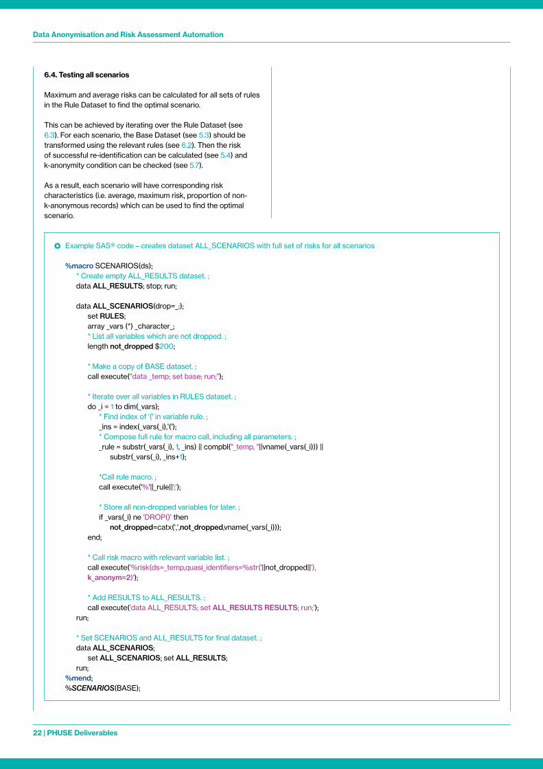
6.4. Testing all scenarios

Maximum and average risks can be calculated for all sets of rules in the Rule Dataset to find the optimal scenario

This can be achieved by iterating over the Rule Dataset (see 6 3) For each scenario, the Base Dataset (see 5 3) should be transformed using the relevant rules (see 6 2) Then the risk of successful re-identification can be calculated (see 5 4) and k-anonymity condition can be checked (see 5 7)

As a result, each scenario will have corresponding risk characteristics (i e average, maximum risk, proportion of non-k-anonymous records) which can be used to find the optimal scenario

Example SAS® code – creates dataset ALL_SCENARIOS with full set of risks for all scenarios

%macro SCENARIOS(ds); * Create empty ALL_RESULTS dataset ; data ALL_RESULTS; stop; run;

data ALL_SCENARIOS(drop=_:); set RULES; array _vars (*) _character_; * List all variables which are not dropped ; length not_dropped $200;

* Make a copy of BASE dataset ; call execute("data _temp; set base; run;");

* Iterate over all variables in RULES dataset ; do _i = 1 to dim(_vars); * Find index of '(' in variable rule ; _ins = index(_vars(_i),'('); * Compose full rule for macro call, including all parameters ; _rule = substr(_vars(_i), 1, _ins) || compbl("_temp, "||vname(_vars(_i))) || substr(_vars(_i), _ins+1);

*Call rule macro ; call execute('%'||_rule||';');

* Store all non-dropped variables for later ; if _vars(_i) ne 'DROP()' then not_dropped=catx(',',not_dropped,vname(_vars(_i))); end;

* Call risk macro with relevant variable list ; call execute('%risk(ds=_temp,quasi_identifiers=%str('||not_dropped||'), k_anonym=2)');

* Add RESULTS to ALL_RESULTS ; call execute('data ALL_RESULTS; set ALL_RESULTS RESULTS; run;'); run;

* Set SCENARIOS and ALL_RESULTS for final dataset ; data ALL_SCENARIOS; set ALL_SCENARIOS; set ALL_RESULTS; run; %mend; %SCENARIOS(BASE);



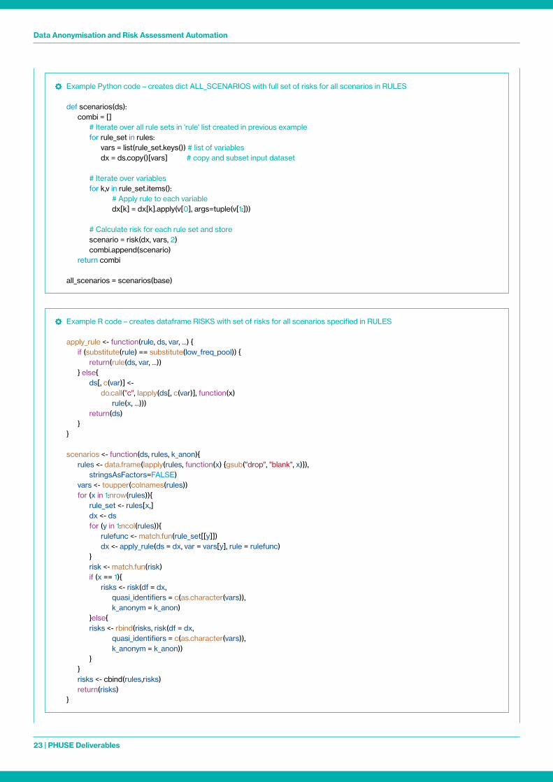
Example Python code – creates dict ALL_SCENARIOS with full set of risks for all scenarios in RULES

def scenarios(ds): combi = [] # Iterate over all rule sets in 'rule' list created in previous example for rule_set in rules: vars = list(rule_set keys()) # list of variables dx = ds copy()[vars] # copy and subset input dataset

# Iterate over variables for k,v in rule_set items(): # Apply rule to each variable dx[k] = dx[k] apply(v[0], args=tuple(v[1:]))

# Calculate risk for each rule set and store scenario = risk(dx, vars, 2) combi append(scenario) return combi

all_scenarios = scenarios(base)

Example R code – creates dataframe RISKS with set of risks for all scenarios specified in RULES

apply_rule <- function(rule, ds, var, ) { if (substitute(rule) == substitute(low_freq_pool)) { return(rule(ds, var, )) } else{ ds[, c(var)] <- do call("c", lapply(ds[, c(var)], function(x) rule(x, ))) return(ds) } }

scenarios <- function(ds, rules, k_anon){ rules <- data frame(lapply(rules, function(x) {gsub("drop", "blank", x)}), stringsAsFactors=FALSE) vars <- toupper(colnames(rules)) for (x in 1:nrow(rules)){ rule_set <- rules[x,] dx <- ds for (y in 1:ncol(rules)){ rulefunc <- match fun(rule_set[[y]]) dx <- apply_rule(ds = dx, var = vars[y], rule = rulefunc) } risk <- match fun(risk) if (x == 1){ risks <- risk(df = dx, quasi_identifiers = c(as character(vars)), k_anonym = k_anon) }else{ risks <- rbind(risks, risk(df = dx, quasi_identifiers = c(as character(vars)), k_anonym = k_anon)) } } risks <- cbind(rules,risks) return(risks) }



6.5. Optimal scenario

In principle, the optimal set of de-identification rules will lead to:

• the average risk being below and closest to the risk threshold,• the proportion of non-k-anonymous records is acceptable

When selecting the optimal scenario, requirements for the prospective analysis should be considered It is possible that some quasi-identifier variables are more “valuable” to the requestor than others

For example, the requestor may prefer to keep maximum level of detail for COUNTRY, at the cost of removing RACE altogether In this case, even if the [COUNTRY(Pool) + RACE(Pool)] scenario results in the risk values closer to the threshold, the subjective data utility will be better for the [COUNTRY(Keep) + RACE(Drop)] scenario

SEX should be prioritised against all other identifiers due to the difficulty in hiding sex in other areas, e g gender-specific adverse events, medication, lab results

It is possible for multiple scenarios to have the same risk score For example, if all subjects are in the same country, replacing COUNTRY with REGION will return the same score The least aggressive rule (KEEP) should always be chosen in such scenarios

6.6. Data utility/information loss metrics

There are several data loss metrics which can assist the selection of optimal scenario The metrics discussed in literature are Discernibility Metric (standard – DM and modified DM*), Non-Uniform Entropy, Optimal Lattice Anonymisation (OLA) The topic is not in scope of this document

6.7. Transform all datasets

Once the optimal set of de-identification rules has been found, corresponding rules must be applied to variables across all datasets

• Unique identifiers must be recoded (pseudonymised) or dropped

• Dates should be offset • Quasi-identifiers need to be transformed per the final rule set • Free-entry and verbatim texts ought to be removed or reviewed-

and-redacted • Any other unwanted variables and values are to be dropped or

cleared

6.8. Convert anonymised datasets to desired format

All programming languages have functions that allow exporting data into many widely recognised formats Depending on the requirements of the request, datasets should be converted to the desired format – SAS7BDAT, XPT, CSV, Dataset xml, XML, JSON, etc Note that changing the format of datasets may change attributes of variables (length, type, etc ) or drop them altogether (label)

6.9. Compile the anonymised package

This task is optional and will depend on the specifications, environment and requirements The following is merely a best practice suggestion

• Compress all parts of the deliverable into a single zip file The package should contain:

• anonymised datasets, • data contents (dataset/variable attributes, classification, de-

identification rule applied), • instructions/assumptions document, • anonymisation report (see 7) • Password protect the package

Different rules may apply when data is shared in secure portals For example, zipping may not be required (protection is embedded in the system, so no need for password protecting files etc )

7. Anonymisation Report

Apart from the anonymised datasets in the desired format and specifications describing the structure of the data and the classification of the variables, the third equally important output is the anonymisation report, which should include:

• list of identifiers (direct and quasi)• classification of all variables and final rules applied to them• description of risk calculation methods (choice of prosecutor/

journalist risk, selection of reference population, etc )• values of risk of attempt (deliberate, inadvertent, breach, overall)• results of risk calculations – to avoid listing all scenarios and

respective risk values, it is advisable to report the risk value of the original dataset (prior to any rules being applied) and the final dataset (with final set of rules applied)

• description of impact on data utility

It may be advisable that any high-level details not relevant for the requestor (specifications, warnings, logs, any subject level information, etc ) be put in an appendix The report can then be included in the package shared with the requestor, but the appendix is never shared and only stored internally with the process documentation

Prior to sharing, the contents of the report should be thoroughly reviewed to avoid inadvertently releasing any sensitive or re-identifying information

Individual steps can contribute to the anonymisation report and outputting parts of report can be programmed into macros and functions for the process steps They can be ultimately collated programmatically to form the bulk of the report, with limited human input required to fill in any gaps



Process in a Nutshell

In its most condensed form, the proposed anonymisation process looks as follows

• Prepare input datasets (2 1)

• Set Thresholds (5 8)

• Assess risk of re-identification attempt – deliberate, inadvertent, breach (5 1)

• Find identifiers in the data, assign classification (3 1)

• Create BASE DATASET by extracting quasi-identifier values for all subjects (5 3)

• Create RULE DATASET by assigning possible rules to each quasi-identifier in BASE DATASET (6 3)

• For each scenario in RULE DATASET:

• Create TRANSFORMED DATASET by applying de-identification rules to BASE DATASET (6 2)

• Calculate risk of successful re-identification (5 5)

• Combine risk of success and risk of attempt to find overall risk of re-identification (5 6)

• Check k-anonymity condition (5 7)

• Store results

• Select optimal (final) rule set based on risk calculations and request requirements (6 5)

• Apply final de-identification rules to all datasets (6 7) and convert to desired formats (6 8)

• Compile anonymised package (6 9)

• Create anonymisation report and add to the package (7)



References and Literature

1 PHUSE De-Identification Standard for SDTM 3.2: Version 1.0, 15-May-2015 accessed at https://www.phuse.eu/white-papers 2 PHUSE Data De-Identification Standard for SDTM 3.2 - Appendix 1: Date Offsetting accessed at https://www.phuse.eu/white-papers3 De-identification and Anonymization of Individual Patient Data in Clinical Studies – A Model Approach accessed at

https://www.phuse.eu/white-papers 4 Institute of Medicine 2015 Sharing Clinical Trial Data: Maximizing Benefits, Minimizing Risk Washington, DC:

The National Academies Press https://doi.org/10.17226/18998 5 El Emam, K (2013) Guide to the De-Identification of Personal Health Information Boca Raton, FL: CRC Press 6 El Emam, K , Arbuckle, L (2013) Anonymizing Health Data: Case Studies and Methods to Get You Started Sebastopol, CA:

O’Reilly Media 7 EU General Data Protection Regulation (GDPR) accessed at:

https://eur-lex.europa.eu/legal-content/EN/TXT/PDF/?uri=CELEX:32016R0679&from=EN8 “United Nations: Standard country or area codes for statistical use (M49)” accessed at


Acknowledgements

Authors:

Lukasz Kniola (Lead), Alex Hughes, Anna Paczewska-Sosnowska, Arlene Coleman, Gregory Campbell, Janine Hodgson, Jasper Enderman, Mahumood Hameed, Jonathan Hartzel, Liam Sheehan, Sarah Hewitt, Terry Walsh PHUSE Data Transparency Working Group

https://www.phuse.eu/documents/working-groups/data-transparency/de-identification/PHUSE-de-identification-standard-for-sdtm-32-version-101-21300.xls

https://www.phuse.eu/white-papers




https://doi.org/10.17226/18998

https://eur-lex.europa.eu/legal-content/EN/TXT/PDF/?uri=CELEX:32016R0679&from=EN


Date post:	27-Jan-2022
Category:	Documents
Upload:	others
View:	5 times
Download:	0 times

Data Anonymisation and Risk Assessment Automation

Documents