204
1 DATA BASE ACCURACY AND INTEGRITY AS A PRECONDITION FOR OVERHEAD ALLOCATIONS Harry H E Fechner Doctor of Philosophy The University of Western Sydney Sydney, Australia 2004

1
DATA BASE ACCURACY AND INTEGRITY AS A
PRECONDITION FOR OVERHEAD ALLOCATIONS
Harry H E Fechner
Doctor of Philosophy
The University of Western Sydney
Sydney, Australia
2004

2
Certification
This is to certify that to the best of my knowledge, the research presented in this
dissertation is my own and original work, except where relevant sections and
references are duly acknowledged. This dissertation has not been submitted
previously in its entirety or substantial parts of it for a higher degree qualification
at any other university or higher educational institution.
Harry H E Fechner
28 January 2004

3
Acknowledgements
There are numerous individuals that deserve special acknowledgment for their
assistance and contribution during the period of my candidature and to them I
express my sincere appreciation. Special thanks must go to my supervisor Assoc.
Prof. Rakesh Agrawal from the University of Western Sydney and co-supervisor
Prof. Graeme Harrison of Macquarie University. I am extremely grateful for the
patience and expert guidance I received from Prof. Agrawal during our many
thought-provoking discussions.
I am also grateful to a number of individuals who provided feedback and
commentary on aspects and content issues of my thesis during presentations at
international accounting conferences. While the list of these individuals is too
numerous, I would like to acknowledge the lengthy discussions I had at various
times with Prof. Malcolm Smith from the University of South Australia, Prof Clive
Emmanuel from Glasgow University, UK, Dr Michael Tayles of Bradford
University, UK, Prof Marc Massoud of Claremont College, California, USA, Prof.
Cecilie Raiborn of Layola University, Louisiana, USA, Prof. Rashid Abdel Khalik,
University of Illinois, USA, Prof Ted Davies, Aston University, UK and Prof Rob
Chenhall of Monash University, Melbourne Australia.
Additional thanks must go to the participants at the various sessions at many
international accounting conferences that provided -through questions and

4
feedback- many thought provoking additional research investigations to include
in the final dissertation.

5
Table of Contents
Certification . . . . . . . . . . . . . . . . . . . . . . . . . . . . . . . . . . . . . . . . . . . . . . . . . . . . . . . 1
Acknowledgements . . . . . . . . . . . . . . . . . . . . . . . . . . . . . . . . . . . . . . . . . . . . . . . . 2
List of Tables . . . . . . . . . . . . . . . . . . . . . . . . . . . . . . . . . . . . . . . . . . . . . . . . . . . . . 6
List of Figures . . . . . . . . . . . . . . . . . . . . . . . . . . . . . . . . . . . . . . . . . . . . . . . . . . . . . 8
Abstract . . . . . . . . . . . . . . . . . . . . . . . . . . . . . . . . . . . . . . . . . . . . . . . . . . . . . . . . . . 9
Executive Summary . . . . . . . . . . . . . . . . . . . . . . . . . . . . . . . . . . . . . . . . . . . . . . . 11
1. The Study Relevance to the Discipline . . . . . . . . . . . . . . . . . . . . . . . . . . 19
1.1 Introduction . . . . . . . . . . . . . . . . . . . . . . . . . . . . . . . . . . . . . . . . . . . . 19
1.2 Contribution of Research to the Discipline . . . . . . . . . . . . . . . . . . . . 29
1.3 Research Objectives . . . . . . . . . . . . . . . . . . . . . . . . . . . . . . . . . . . . . 31
1.4. Research Methodology and Methods . . . . . . . . . . . . . . . . . . . . . . . . 33
1.4.1 Mathematical Techniques employed for model development. . 35
1.5 Structure of Thesis . . . . . . . . . . . . . . . . . . . . . . . . . . . . . . . . . . . . . . 40
1.6 Definitions, Key Assumptions and Limitations. . . . . . . . . . . . . . . . . . 40
Definitions . . . . . . . . . . . . . . . . . . . . . . . . . . . . . . . . . . . . . . . . . . . . . 40
Key Assumptions . . . . . . . . . . . . . . . . . . . . . . . . . . . . . . . . . . . . . . . . 43
Limitations . . . . . . . . . . . . . . . . . . . . . . . . . . . . . . . . . . . . . . . . . . . . . 44
2. Literature Review . . . . . . . . . . . . . . . . . . . . . . . . . . . . . . . . . . . . . . . . . . . . 46
2.1 Introduction . . . . . . . . . . . . . . . . . . . . . . . . . . . . . . . . . . . . . . . . . . . 46
2.1.1. Traditional Organisational and Operational Environments . 48
2.2.2 The Full Cost (or Absorption Cost) Concept. . . . . . . . . . . . . . 51
2.2.3 The Variable Cost (or Direct Cost) Concept. . . . . . . . . . . . . . 59
2.2.4 Standard Cost Concept . . . . . . . . . . . . . . . . . . . . . . . . . . . . . 61
2.2 The Changing Organisational and Operational Environments. . . . . . 63
2.2.1 Activity-Based Costing . . . . . . . . . . . . . . . . . . . . . . . . . . . . . . 66
2.2.2 The Theory of Constraints . . . . . . . . . . . . . . . . . . . . . . . . . . 74
2.2.3 Strategic Management Accounting . . . . . . . . . . . . . . . . . . . . . 79
2.2.3.1 Critical Evaluation of Emerging
Management Accounting Systems . . . . . . . . . . 83
2.2.3.2C Case Study Based Comparison between
ABC and MAS. . . . . . . . . . . . . . . . . . . . . . . . . . 83
2.2.3.3 Error Incidence and System Accuracy . . . . . . . 92
2.2.3.4 The (IR)Relevance of Cost Management
Systems . . . . . . . . . . . . . . . . . . . . . . . . . . . . . 102
2.3 Chapter Summary . . . . . . . . . . . . . . . . . . . . . . . . . . . . . . . . . . . . . . 117

6
3. Model Development. . . . . . . . . . . . . . . . . . . . . . . . . . . . . . . . . . . . . . . . . 119
3.1 Introduction . . . . . . . . . . . . . . . . . . . . . . . . . . . . . . . . . . . . . . . . . . . 119
3.1.1. Database Integrity . . . . . . . . . . . . . . . . . . . . . . . . . . . . . . . . 122
3.2 Development of a Pareto Frontier Model. . . . . . . . . . . . . . . . . . . 125
3.3 Data Base Generation and Pattern Recognition . . . . . . . . . . . . . . . 132
3.4 Chapter Summary . . . . . . . . . . . . . . . . . . . . . . . . . . . . . . . . . . . . . . 150
4. Case Study Analysis . . . . . . . . . . . . . . . . . . . . . . . . . . . . . . . . . . . . . . . . . 151
4.1 Introduction . . . . . . . . . . . . . . . . . . . . . . . . . . . . . . . . . . . . . . . . . . . 151
4.2 Case Study Analysis Stock Exchange Data. . . . . . . . . . . . . . . . . 154
4.2 Case Study Analysis University Enrolment Data . . . . . . . . . . . . . . 156
4.3 Case Study Analysis Inventory Data . . . . . . . . . . . . . . . . . . . . . . . . 166
4.4 Chapter Summary . . . . . . . . . . . . . . . . . . . . . . . . . . . . . . . . . . . . . . 173
5. Discussion of Results . . . . . . . . . . . . . . . . . . . . . . . . . . . . . . . . . . . . . . . 176
6. Summary and Future Research Suggestions . . . . . . . . . . . . . . . . . . . . 185
6.1 Summary . . . . . . . . . . . . . . . . . . . . . . . . . . . . . . . . . . . . . . . . . . . . . 185
6.2 Major Contribution . . . . . . . . . . . . . . . . . . . . . . . . . . . . . . . . . . . . . . . 193
6.3 Future Research Suggestions . . . . . . . . . . . . . . . . . . . . . . . . . . . . . 194
References . . . . . . . . . . . . . . . . . . . . . . . . . . . . . . . . . . . . . . . . . . . . . . . . . . . . . 196
List of Publications by Author relating to Thesis . . . . . . . . . . . . . . . . . . . . . . 202

7
List of Tables
TABLE 2-1 A summary of surveys: elements of cost . . . . . . . . . . . . . . . . . . . . . . . . . . 50
TABLE 2-2 [Period 1](Product unit data) . . . . . . . . . . . . . . . . . . . . . . . . . . . . . . . . . . . 53
TABLE 2-3 [Period 2](Product unit data) . . . . . . . . . . . . . . . . . . . . . . . . . . . . . . . . . . . 54
TABLE 2-4 [Period 3](Product unit data) . . . . . . . . . . . . . . . . . . . . . . . . . . . . . . . . . . . 55
TABLE 2-5 Comparison between MAS and ABC overhead allocations . . . . . . . . . . . . 89
TABLE 2-6 Regression result of Total Overhead on Direct Labour Costs . . . . . . . . . . 91
TABLE 2-7 Error incidence in [abc] product costing approach . . . . . . . . . . . . . . . . . . . 94
TABLE 2-8 (Product data taken from Pattinson and Arendt (1994:61)) . . . . . . . . . . . 100
TABLE 2-9, Product data . . . . . . . . . . . . . . . . . . . . . . . . . . . . . . . . . . . . . . . . . . . . . . 105
TABLE 2-9a Product cost and contribution margin data . . . . . . . . . . . . . . . . . . . . . . . 106
TABLE 2-9b Cost Pool data using different cost drivers . . . . . . . . . . . . . . . . . . . . . . . 107
TABLE 2-10 Example (Set-up cost pool) of individual product activity cost calculations 108
TABLE 2- 11 Constraint Equations . . . . . . . . . . . . . . . . . . . . . . . . . . . . . . . . . . . . . . . . 109
TABLE 2- 12 Results report of LP analysis . . . . . . . . . . . . . . . . . . . . . . . . . . . . . . . . . 111
TABLE 2-13 Profitability under varying product mix selections . . . . . . . . . . . . . . . . . 113
TABLE 2-14 Opportunity costs under different product mix constraints. . . . . . . . . . . . 114
TABLE 3-1 Results of ANOVA for data distribution of 8 (500 items) data bases . . . 135
TABLE 3-2 Results of ANOVA for data distribution of 8 (1000 items) data bases . . 136
TABLE 3-3 Results of ANOVA for data distribution of 8 (2500 items) data bases . . . 137
TABLE 3-4 Results of ANOVA for data distribution of 8 (4000 items) data bases . . 138
TABLE 3-5 Error data for Incremental and Point Differences . . . . . . . . . . . . . . . . . . . . . .141
TABLE 3-6 Results of ANOVA for data distribution of 5 random selected data
bases from the 500, 1000, 2500 and 4000 items data bases
with varied parameters for price, demand and shape factor. . . . . . . . . . . 149
TABLE 4-1, Results of ANOVA for Australian Share data("=.05) . . . . . . . . . . . . . . . . 155
TABLE 4-1a F-test for daily transactions/model values("=.05) . . . . . . . . . . . . . . . . . . 155
TABLE 4-3 (University 13) Results of ANOVA for 5 year DEST data ("=.05) . . . . . . 158
TABLE 4-4 (University 13) F-test for yearly enrolment records/model values (("=.05) 158
TABLE 4-5 ANOVA for each of the 12 universities’ 5 year students enrolment records160
TABLE 4-6 (University 1) F-test for yearly enrolment records/model values (("=.05) 161
TABLE 4-7 (University 2) F-test for yearly enrolment records/model values (("=.05) 161
TABLE 4-8 (University 3) F-test for yearly enrolment records/model values (("=.05) 161

8
TABLE 4-9 (University 4) F-test for yearly enrolment records/model values (("=.05) 161
TABLE 4-10 (University 5) F-test for yearly enrolment records/model values (("=.05) 162
TABLE 4-11 (University 6) F-test for yearly enrolment records/model values (("=.05) 162
TABLE 4-12 (University 7) F-test for yearly enrolment records/model values (("=.05) 162
TABLE 4-13 (University 8) F-test for yearly enrolment records/model values (("=.05) 162
TABLE 4-14 (University 9) F-test for yearly enrolment records/model values (("=.05) 163
TABLE 4-15 (University 10) F-test for yearly enrolment records/model values (("=.05) 163
TABLE 4-16 (University 11) F-test for yearly enrolment records/model values (("=.05) 163
TABLE 4-17 (University 12) F-test for yearly enrolment records/model values (("=.05) 163
TABLE 4-18 Results of ANOVA for Inventory data("=.05). . . . . . . . . .. . . . . . . . . . . . . . . . .167
TABLE 4-18a F-test for Model/Inventory("=.05) . . . . . . . . . . . . . . . . . . . . . . . . . . . . . . . 167
TABLE 4-19 Model parameters for Case study data . . . . . . . . . . . . . . . . . . . . . . . . . . 169
TABLE 4-20 Cost Allocation Variances (Actual v Confidence Limits) . . . . . . . . . . . . 171

9
List of Figures
FIGURE 1-1 Fechner’s Strategic Management Accounting Framework . . . . . . . . . . . . . 27
FIGURE 1-2 Framework for Thesis Structure . . . . . . . . . . . . . . . . . . . . . . . . . . . . . . . . . 39
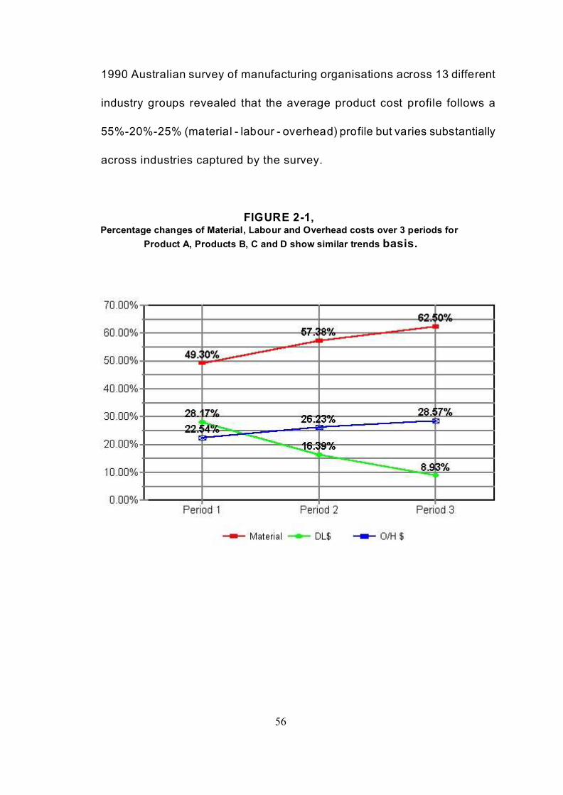
FIGURE 2-1 Percentage changes of Material, Labour and Overhead costs over
3 periods for Product A, Products B, C and D show similar trends basis. 56
FIGURE 2-2, Percentage changes of Material, Labour and Overhead costs over
3 periods for Product A as proportion of the selling price; Products B, C
and D show similar trends basis . . . . . . . . . . . . . . . . . . . . . . . . . . . . . . . . 57
FIGURE 2-3 (Fig. 1-1 repeated here for clarity) Strategic Management Accounting
Framework . . . . . . . . . . . . . . . . . . . . . . . . . . . . . . . . . . . . . . . . . . . . . . . . . 82
FIGURE 2-4 Pareto Frontier, sorted by Direct Labour Hours . . . . . . . . . . . . . . . . . . . . . 85
FIGURE 2-5 Product over/under overhead distribution for the JDCW data . . . . . . . . . . 87
FIGURE 2-6 ABC compared to Traditional MAS Product Cost Portfolio . . . . . . . . . . . 101
FIGURE 2-7 Activity Cost Variation [Benchmark - ABC] . . . . . . . . . . . . . . . . . . . . . . . 110
FIGURE 3-1 Data Base and Model Comparison . . . . . . . . . . . . . . . . . . . . . . . . . . . . . 142
FIGURE 3-2 Typical Incremental Error Distribution . . . . . . . . . . . . . . . . . . . . . . . . . . . 143
FIGURE 3-3 Error Distribution of Point Estimates . . . . . . . . . . . . . . . . . . . . . . . . . . . . 145

10
Abstract
Interest in more accurate assignment of overhead costs to establish credible
product/service cost profiles has assumed substantial prominence in much of the
recent debates on management accounting practices. While the promotion of
“new” cost management systems and in particular Activity Based Costing [ABC]
has promised to address many of the perceived shortcomings of more traditional
and long established techniques, the lack of its implementation success raises
some concern as to the validity and value of these “new” system designs.
Survey evidence from a number of different sources involving the evaluation of
past and current practices seem to identify the continued usage and application
of traditional cost management techniques and furthermore support a preference
by management to rely on simplistic allocation models for overhead cost
assignments. An often criticised limitation of the traditional absorption cost
system, the most popular in the survey findings, has been its reliance on a single
volume based cost driver (mostly Direct Labour Hours, DLH) for allocating
overhead costs. As organizations increasingly have employed advanced
technologies in many of their operational domains, DLH may no longer represent
a sound proxy for these allocations.
A major purpose of this thesis is the development of a mathematical model that
is capable of computing overhead allocations on the basis of organisational

11
specific dimensions other than DLH. While almost all data bases suffer from data
entry and omission errors, the information content contained in the data bases
often forms the basis for management decisions without first confirming the
accuracy of the data base content. The model has been successfully applied and
tested to detect internal consistency and data element detail accuracy. A total of
3200 random number generated data bases with varying number of elements as
well as characteristics that typify general inventory data base records were tested
and statistically evaluated to confirm the validity of the model. It was found to be
robust under all the subjected varying parameters and therefore able to detect
domain consistencies and data element inconsistencies.
Future research may test the applicability of the model with more diverse data
bases to confirm its generalisability as an investigative as well as predictive
model.

12
Executive Summary
This thesis has developed a mathematical model that mirrors the general pareto
or unbalanced distribution of data base elements given pre-specified element
parameters. To test the model’s robustness, standard statistical analysis (ANOVA
and F-test) of comparing paired elements between random number generated
data and model computed data, as well as incremental data comparisons
revealed non significant outcomes, thereby confirming the validity of the model to
detect data base inconsistencies.
Data mining of existing data bases revealed pattern consistency over a number
of periods that allowed the application of the model to detect data base integrity
or domain consistency (data belonging to the same organisation over a number
of periods) and data element accuracy (empirical evidence identified the
existence of data element errors through inaccurate entry or omissions) by
comparing the existing data base elements with the model generated data.
A further contribution of the thesis is the application of the model to identify data
base errors in an organisation’s inventory and production records and applying the
model’s generated values for the allocation of overhead costs. This concept of
overhead allocations parallels the simplicity of the traditional absorption technique
but increases the accuracy of the allocation method. This application is not limited
to manufacturing organisations but can be equally well applied to service
organisations.

13
Overhead allocations have consistently been criticised as arbitrary, incorrigible
and misleading in determining accurate product costs. Literature evidence, both
article and textbook based, often presents examples in which the overhead cost
component exceeds 45% of total product costs. Under these circumstances, any
different method (new?) of overhead allocations (assignment, distribution)
produces convincing results for consideration of such new methods, e.g ABC
costing methods. Surprisingly, a number of recent surveys of manufacturing
industries in different countries found that the average proportion of both
manufacturing and non-manufacturing overheads combined is around 30% (Drury
and Tayles, 1994; Joyce and Blaney, 1990; Dean et at., 1991). At this level, the
perceived benefit from a "more accurate" cost assignment method is substantially
reduced, which might explain that reported survey results on the subject of
overhead allocations often find no significant modifications to existing
Management Accounting System [MAS] practices.
While the debate about alternative management accounting systems remains a
contemporary issue amongst academics and practitioners alike, the most popular
of the suggested alternatives, Activity Based Costing [ABC], has had only limited
success when compared with the continued application of traditional MAS
techniques (Shim and Sudit, 1995). Survey results on the adoption and
implementation of ABC indicate that, in countries like the US, UK, Canada,
Australia, Japan and some European countries, the acceptance/implementation

14
rate varies between 6% and 12% across the industry spectrum (Cobb et al.,1993;
Cooper et al, 1988; Drury and Tayles, 1994; Dean et al., 1991; Fechner, 1995;
Armitage and Nicholson, 1993).
A persistent problem mentioned in the literature on ABC implementation is the
substantial cost involved in maintaining the system apart from the initial costs of
implementation. Other comments have questioned the benefits of more “accurate”
product costs as some of the overhead allocation problems remain and require
similar subjective judgmental allocations as experienced in traditional MAS
(Kaplan, 1994a).
Furthermore, anecdotal evidence and testimonials question the benefit of a
system replacement that is difficult to assess as to its final value. In addition the
initial operational analysis as to the totality of all value adding activities and the
determination of appropriate cost drivers presents many managements with
system complexities that are difficult to conceptualise as to the overall
improvements that can be achieved. This overwhelming complexity of the
activity/cost driver matrix and the extent of the organisation’s product range are
recurring comments throughout much of the related literature in identifying the
reluctance by management to implement an ABC system.

15
The premise of any of the proposed “new” systems is that the organisation will
benefit from better decision support systems and thereby ultimately improve
profitability. Although this premise is defensible, its validation can only be
supported if the organisation’s current operations are well within its existing
resource capacities. To demonstrate this proposition, an example of capacity
(operational) constraints for a given product mix is submitted to optimisation
analysis (Theory of Constraints). This example tests the usefulness of a number
of alternative overhead cost allocation systems to provide evidence for the
indifference that any of these systems offer in determining an organisation’s
optimal profitability.
Most of the operational analyses that precede the evaluation and subsequent
implementation relies on an organisation’s existing data bases. However, there
also seems to be a reliance on data base integrity without the necessary
verification for such assumption. One of the discernible characteristics of almost
all data bases is their unbalanced distribution of element items when ranked on
the basis of two dimensions of interest.
Alfredo Pareto was the first scholar to recognise such relationships and since his
introduction of this phenomenon subsequent writings on the subject have referred
to it as the Pareto principle or the 80/20 rule. A well known application of the
80/20 rule within the accounting domain is the A-B-C classification employed in

16
inventory control system design. Identifying products on the basis of their
individual value in relation to the total value of inventories provides a sound
approach for determining the resources to be expanded in controlling a major
asset in most organisations. An extension to this product classification as to the
individual product value within the total product portfolio would be to analyse if the
product cost profiles follow a similar distribution with particular emphasis on the
overhead proportion. While it is hypothesised that the resource consumption of
products parallels this of the inventory classification ranking, normal statistical
analysis is applied to support such conjecture.
Chapter 3 covers the major contribution of this thesis. The development of a
mathematical model to determine the exact 80/20 relationship (or any other
combination) on the basis of the total number of products. Such a computational
model provides the analyst (management accountant) with a tool to determine the
individual product contributions and thereby assists in establishing a hypothetical
benchmark for resource comparison. Although such a model is useful in
determining the hypothetical resource allocations, and therefore a benchmark, the
model does not, however, identify any existing inefficiencies in product or process
design. The model developed (as shown):

17
where P = total number of products in portfolioxi = ith product rank within portfolioyi cum = cumulative percentage of ith product contributionc = constant for a given data base.(xi/P)d = term that determines the shape parametere = base of natural logarithm (2.718281)
is capable of identifying existing data base inaccuracies that indicate domain
consistency and data item inconsistencies, therefore providing a sound basis for
data element attribute predictions. As the interest of the thesis is in comparing the
usefulness of existing overhead allocations methods, the model will be applied in
computing overhead allocations based on its pair wise comparison with the actual
data of an organisation’s inventory and production records. The benefit provided
by such overhead allocation method, is its application simplicity as well as the
accepted - but criticised - absorption costing method.
In chapter 4, three specific data bases (case studies) have been selected for their
perceived data integrity and to test the robustness of the model against actual,
rather than random number generated, data bases. Statistical analysis establishes
the accuracy of data element attributes as well as identifying domain
consistencies. While the outcome of the analysis was hypothesised, the results
were still somewhat surprising.

18
Stock Exchange daily transaction data should be audited prior to its release into
the public arena and therefore display a high level of data accuracy. The data
contained inaccuracies that were explained by the providers of the data records
as rounding applications of nonmarketable securities.
Australian university data of student enrolments on the other hand is often
presented unaudited to governmental funding authorities and thereby invites
suspicion as to the accuracy of the data recorded. Again data analysis revealed
both domain inconsistencies and data item inaccuracies.
The third case study is a current research study in which the organisation is
preparing to implement an ABC system that has been imposed by its European
based parent company. Many of the pre-requites of system change over were not
well understood by the operations personnel and the existing system has no
separate overhead classification but a rather inappropriate single conversion cost
distribution by cost centre. The application of the developed model identified
existing data base inaccuracies and provided operations management of the
organisation with evidence of data entry and omission errors for investigation and
correction where appropriate.
Chapter 5 discusses in detail the analysis of error terms from the 3200 random
number generated data bases its implications and application to the inventory and

19
production data base. It further provides application specific statistical error term
calculations that are necessary for the computation of data element parameters.
The final chapter provides a summary and direction for future research in the area
of model extension and resource efficiency improvements.

19
1. The Study Relevance to the Discipline
1.1 Introduction
Early research investigating the effect of technology on organisational
design suggested that organisational structure will experience modifications
with the implementation and use of technologies (Woodward, 1965;
Perrow, 1967; Thompson,1967; Duncan, 1972). However, to modify and
then maintain those structures, control systems have to be designed to
achieve these objectives. The realisation of the existence of organisational
design interdependencies lead to the development of contingency theory
(Gordon and Miller, 1975; Hayes, 1983; Waterhouse and Tiessen, 1978).
Organisational theorists embraced this new framework as it had the
promise of explaining a large number of organisational variables and their
interdependencies.
From the basis of the contingency model a number of diverse studies were
conducted to support the hypothesised relationships between selected
variables. Technology, as one of the organisational variables of interest in
explaining organisational design changes, became a credible explanation
for the operations structural changes and the need to match control system
design with the new operational environment (Daft and Mclntosh, 1978;
Merchant, 1984; Mclntosh and Daft, 1987). The latter aspect has created
a substantial body of research with divided opinions about the relevance of

20
management accounting systems in these new Advanced Manufacturing
Technologies [AMT] production environments (Kaplan, 1983, 1986b;
Johnson and Kaplan, 1987). There is, however, an equally substantial body
of research that argues in favour of retaining the traditional management
accounting techniques in modified forms to match the organisation’s
information needs (Drucker, 1990).
Traditional management accounting practices have received increasing
attention from accounting academics who question the relevance of these
traditional practices in an environment of expanding advanced technology
based production. Kaplan (1983, 1984, 1986a,1988, Johnson and Kaplan,
1987) has become the most prominent and vociferous critique of the
management accounting irrelevance movement. His contention is largely
based on anecdotal and case study testimonials, suggesting that, with the
advent of large scale adaptation of Advanced Manufacturing Technologies
by manufacturing industries, the function of traditional Management
Accounting Systems [MAS] as a tool for planning and control is no longer
defensible. He attributes this diminished functional role of MAS to the lack
of perceived independence from the financial accounting function.
This argument has some credibility, especially if the origin and
development of many of the currently practiced management accounting

21
techniques can historically be traced to the scientific management era. It
was in this environment that production engineers developed most of our
contemporary management accounting techniques (Kaplan, 1986a).
Therefore, it appears to be quite reasonable to again consult with
production engineers and planners to gain a better understanding of what
type of operational measurement requirements are needed in an AMT
environment. Management accountants thereby have some obligation to
become more familiar with production operations to develop appropriate
modifications to existing MAS.
The adoption and implementation of AMTs by organisations are driven by
the organisation's desire to gain or maintain a competi tive advantage
whereby consumer needs of constant high quality products or services at
competitive prices become the motivating objective. To meet this dual but
previously sought to be mutually exclusive criteria, firms have concentrated
on cost reductions often in the areas of direct and indirect labour costs. The
product cost profile of organisations who have implemented some form of
AMT should therefore indicate a shift in the components of the product cost
profile. Furthermore, recent surveys (Drury and Tayles, 1994; Joyce and
Blaney, 1990) have indicated that differences in product cost components
between various industry groups exist.

22
Such differences may also be indicative of the treatment of product cost
determinations within different industries and provide some information on
the overhead allocation methods applied. Overhead allocations have
consistently been criticised as arbitrary, incorrigible (Thomas, 1975) and
misleading in determining accurate product costs. Surprisingly, a number
of recent surveys of manufacturing industries in different countries found
that the average proportion of both manufacturing and non-manufacturing
overheads combined is less than 30% (W hittle, 2000; Drury and Tayles,
1994; Joyce and Blaney, 1990, Dean et al., 1991). At this level, the
perceived benefits from a "more accurate" cost allocation method are
substantially reduced, which might explain that reported survey results on
the subject of overhead allocations often find no significant modifications
to existing MAS practices.
However, if the overhead component constitutes only some 30% of the total
product costs, given the evidence of recent surveys, the question arises at
what level of overhead proportion will the traditional allocation methods
become questionable and jeopardise the value of information that is
conveyed to management for product related decision making. Literature
evidence, both article and textbook based, often presents examples in
which the overhead cost component exceeds 45% of total product costs.
Under these circumstances a different method of overhead allocations

23
produces convincing results for consideration of such new methods, e.g
ABC costing methods. Activity-based-cost [ABC] overhead allocations, a
method popularised by academics and consultants as an alternative to
traditionally based allocations methods, lacks the universality of application
as it depends largely on product diversity and product level overhead cost
pools (Cooper, 1988).
It is encouraging to note the recent change in management accounting
thought toward strategic cost management. This relatively new approach
to the traditional management accounting practices provides a desired
integrative framework for linking management accounting, operations
management and strategic management to create a cohesive group of
functional activities. W ithin this framework, technology is regarded as a
consequence of strategic choices and management accounting systems
are tools that aid in the implementation of those strategies (Govindarajan
and Shank, 1990).
Strategic management accounting [SMA], is a relatively new development
in understanding the relationships that dominate organisational design and
its maintenance mechanisms through the appropriate application of
internal control systems. It has been advanced as the natural progression
of earlier contingency theory prescriptions. While the underlying

24
assumptions of this approach are not new, the framework does however,
recognise the functional interrelationships of strategic management,
operations management and management accounting (Govindarajan and
Shank, 1990). It further identifies the relative importance of product life
cycle [PLC] analysis as a linking mechanism between strategic choice and
supporting management accounting system designs.
Much of the MAS irrelevance debate (Kaplan, 1983, 1986b, 1988; Johnson
and Kaplan, 1987) has been concentrating on the lack of modification to the
traditional management accounting practices in organisations after the
implementation of some form of an AMT. The main arguments are based
on the presumption that AMTs tend to reduce the direct labour content as
a proportion of total product costs and at the same time substantially
increase the proportion of manufacturing overheads. The allocations of the
presumed increased overheads on traditional based labour costs as well
as capacity volume related distributions are considered to provide
inaccurate cost data for product related decisions (make v buy, retain or
abandon, product mix, etc.) and it is argued that for these reasons they
have lost their relevance as a management decision support system.
As Kawada and Johnson (1993) point out the difference between the
”accuracy school” represented by ABC advocates and strategic

25
management accounting is the emphasis each of these “schools” attach to
organisational issues.
Whereas the accuracy movement stresses that the internal product cost
accuracy leads to improved profitability, the strategic movement stresses
that the analysis of the external environment mandates corrections and
adjustments to the internal control system structures and decision support
systems. Both movements, however, tend to agree that the traditional
financial based cost management system is no longer appropriate for either
task.
To provide a clearer example of the differences in the way of thinking these
schools represent can best be demonstrated by the product/services
related questions they address. The ABC school (internal focus)
emphasises improved profits through accurate product/service costing
while the strategists (external focus) are preoccupied with the question of
what products the company should produce.
The relevance of either emphasis may be revealed by the strategic stance
the company adopts with regard to cost leadership or product/service
differentiation. Therefore, accepting that both schools of thought have a
valuable contribution to make to the survival and growth of organisations

26
requires the development of techniques that combine the assessment of
product cost profile accuracy with the evaluation of product desirability and
viability. The literature in general has treated each of these emerging
issues as separate and distinct paradigms with specific contributions to the
overall functioning of organisations. However, there seems to be a
considerable commonality between these issues and represents an
opportunity to develop a linkage that offers a synergy between them.
In a contemporary survey (Shields and McEwen, 1996) it was found that the
successful implementation of ABC, amongst other factors, is dependent on
linking it to the “company’s competitive strategy regarding organizational
design, new product development, product mix and pricing and technology”
(p.18). However, while the authors offered a number of examples where
such a linkage would be beneficial, there was no suggestion as to the
concept or operational technique that would promote such
interdependence. A common thread that links all company objectives is the
realisation that available resources are limited and that these limitations
impose resource constraints that require efficient management.
To evaluate the effect resource constraints impose on the optimisation of
the organisation’s objectives, a number of operations management
techniques have been available for some time, most prominent amongst
them is the Theory of Constraints (ToC).

27
FIGURE 1-1
Fechner’s Strategic Management Accounting Framework
As the term suggests, [ToC] is based on the concept that the main objective
for efficient organisational functioning is to achieve resource optimisation
by attenuating the demand for a firm’s products/services with its flow of
production including administrative and other supporting functions.
However, most traditional and “new” management accounting systems do
not consider the optimisation of physical and resource capacities when
determining appropriate cost assignments to individual products.
The analysis of an organisation’s external environment to assess its
comparative advantage (to answer questions as to what products should

28
be produced) must be linked to the organisation’s capacity to produce these
products efficiently and within the expected cost boundaries. Figure 1-1
illustrates these interrelationships and how the consolidation of the
“accuracy” and “strategy” schools form the foundation of the strategic
management accounting discipline that leads to the determination of an
organisation’s product/service portfolio.
The determination of an organisation’s optimal product/service mix requires
the utilisation of optimality models. Most common amongst these are
Linear [LP] and Mixed Integer programming [MIP] applications. For a more
detailed discussion refer to Kee and Schmidt (2000). Although, the TOC is
sometimes criticised for relying on deterministic assumptions and thereby
reducing its value in predicting product mix compositions, stochastic
models are less appropriate as “production related activities are
deterministic in nature” (Kee and Schmidt 2000:5). The authors further
suggest that neither the ABC model nor the TOC model will be able to
compute an optimal product mix when both labour and overhead costs are
of a discretionary nature but that their general model (Mixed Integer
Programming, MIP) computes an optimal product mix.
This analysis provides an opportunity to discover that profit optimisation is
dependent on capacity utilisation and/or market demand constraints which

29
illustrate that cost accounting systems of whatever design will have no
influence on the profitability outcome of the organisation (refer to Table 2.9,
2.9a, and 2.9b). Such results may help to explain the continued popularity
of traditional cost accounting techniques and the reluctance by
managements’ to implement contemporary systems such as Activity-Based
Costing.
This generalisation, however, needs to be moderated as it is difficult to
apply optimality models organisation wide and maybe restricted to the
analysis of functional units within the corporate framework.
Rather then suggesting that cost management systems are irrelevant when
determining an organizations profitability, the difficulty in implementing
optimality analysis corporate wide, refocuses the emphasis on cost
accounting systems capable of assigning or allocating overhead costs to
individual products/services on a credible basis.
1.2 Contribution of Research to the Discipline
Survey results (Drury and Tayles, 1994; Joyce and Blaney, 1990; Dean et
al., 1991; Fechner, 1995; Whittle, 2000) as well as a historical review
(Boer, 1994) clearly indicate that overhead cost proportions within a
product’s cost profile have not substantially changed over time and

30
organisations continue to prefer simplistic overhead allocation methods.
Although some of the evidence suggests that traditional allocation models
produce some inequitable overhead allocations within the organisation’s
total product portfolio it appears to be more appropriate to develop an
overhead allocation method that incorporates the changing environmental
circumstances but maintains the simplicity of an overall overhead allocation
method.
A major problem that has not been addressed by previous research is the
accuracy and integrity of organisational data bases that form the basis for
cost accumulation and subsequent cost allocations. Incomplete or
inaccurate cost accumulation pools may contribute to the claimed cost
distortions that have been identified in comparative cost management
system examples and case studies.
To address the dual problems of data base integrity and more equitable
overhead cost allocations this thesis will adopt a data mining technique to
identify data patterns within random number generated data bases from
which a predictive model can be developed. This model will then be tested
for its robustness against publicly available stock exchange data,
Australian university student enrolment records and company data bases.
Statistical tests to evaluate the model parameters against the actual data
will be applied to confirm its predictive value in determining overhead cost
allocations.

31
1.3 Research Objectives
This thesis will:
- develop a robust model for the allocation of overheads that is
based on the historical data pattern of the company’s
inventory and production records.
- analyse and test the commonal ity of data base patterns to
confirm the empirical evidence as to the existence of the
Pareto distribution - or 80/20 rule - in a number data bases.
- develop a mathematical model that mirrors the data
distribution of Pareto ranked cumulative element
arrangements to test its robustness under varying parameters.
To test such robustness standard statistical analysis of paired
element comparisons (Anova and F-test) as well as error term
analysis for incremental values and point estimates will be
conducted.
- identify data base integrity and data accuracy (as empirical
evidence suggests that almost all data bases contain data
element errors through inaccurate entry and omissions) by
comparing the initial data base with the model generated data
base for pattern consistency.
While the model will have universal applicability its parameters need to be
determined on the data pattern history of the individual organisation. By
32
accepting that each data base will have its unique pattern, it is
hypothesised that the data pattern within a given domain (organisation) will
display pattern consistency while such consistency is not expected across
different domains even within the same industry grouping.
If such findings are revealed by the analysis then a further benefit from the
model would be its ability to detect pattern inconsistencies within a domain
as unexpected and alert appropriate management levels to the possibility
of data errors and inaccuracies.
Once the data base integrity of a domain has been established, the model
will be applied to compute individual product overhead cost allocations on
the basis of the ranked data base element distribution of pre-specified
product attributes. Such pre-specified product attributes could include
product demand, material consumption and resource consumption amongst
others.
33
1.4. Research Methodology and Methods
Most data bases display nonlinear relationships between any dual content
data items of interest. Steindl (1965:18) recognised this fact and stated that
“for a very long time, the Pareto law [ the 80/20 principle] has lumbered the
economic scene like an erratic block on the landscape; an empirical law
which nobody can explain.” While this observation in itself does not provide
any new insights into the existence of such phenomenon, it does, however,
provide an opportunity to quantify through mathematical modelling the
individual data item contribution to the distinctive shape of the cumulative
distribution curve.
The application of the Pareto principle relies on the availability of a data
base that constitutes the population of data items of interest. Ranking of
items on the basis of two dimensions of interest will produce a typical
Pareto distribution. The development of a model that can mirror the Pareto
frontier produced by the ranking of data items, will allow the application of
such a model as a prediction tool of the items of interest. The purpose of
this thesis is to use mathematical modelling techniques to develop such a
model and apply it in the prediction of overhead costs for a company’s
product portfolio.

34
The development of the model required the testing of the specified model
parameters against a substantial number of data bases to ensure that it has
the robustness required to become a credible prediction tool.
The initial database testing will use a substantial number of random number
generated data bases with different data item populations. These data
bases will contain typical product cost characteristics where each of the
cost components of material, direct labour and overhead allocations are
randomly varied. To accomplish this task, a standard spreadsheet
application (Quattro Pro in this case) will be employed which has the
desired random number generator function to establish the database
combinations. Although there is no relevant literature to provide guidance
as to the population size required for mathematical modelling, a reasonable
population size that mirrors average inventory holdings of manufacturing
organisations in the range from 500, 1000, 2500 and 4000 items would
appear to be adequate. For each of the populations 100 random number
generated data bases ( a total of 3200 populations) will be compared with
the developed model to establish a statistically adequate sample size. To
further improve on the robustness of the model, an error term (deviation
between model computed values and database values) of +/- 5% in the fat
tail region of the distribution is considered appropriate. This level is
suggested as an acceptable error term as most standard statistical tests of
significance are set at a 5% level for model prediction validity.

35
The model will be tested against each random generated data base to
calculate the error term of its parameters against the item values of the
data base. A paired comparison using single ANOVA statistics together
with a standard F test will be used to establish the validity of the model
parameters.
1.4.1 Mathematical techniques employed for the model development
For the development and application of the model a number of
mathematical techniques were used to establish data base pattern
consistency as well as the analytical evaluation of existing overhead
assignment techniques. To establish the existence of a generalised Pareto
distribution (GPD) as suggested by Koch (1998) existing data bases need
to be investigated for pattern similarities in a data mining approach.
Data mining in the context of this thesis refers to the investigation of
appropriate existing data bases (populations), given some pre-determined
parameters or element characteristics, to identify data element patterns that
confirm the general accepted but anecdotal evidence of the Pareto principal
or unbalanced distribution.
The Pareto principal or unbalanced distribution should not confused with
the theoretical Pareto optimality concept. Pareto optimality is achieved

36
when the distribution of goods/services falls on the contract curve in a
modeled Edgeworth-Box diagram and represents the condition of optimal
resource/commodity/welfare distribution. The exchange of goods/services
beyond a point on the contract curve leads one consumer to be worth of in
his (her) indifference towards a bundle of goods/services. Although the
concept can also be applied to the production possibility frontier
hypothesis, it is not the purpose of this thesis to deal with the economic
rationale of Pareto optimality but instead introduces the concept of Pareto
efficiency in which a vital few and not the trivial many affect the output
condition of the firm.
Pareto’s original discovery of the wealth distribution in a certain population
followed a 20/80 pattern (20% of the population enjoyed 80% of the
wealth). Further investigation by Pareto (Koch, 1998:6) revealed that this
unbalanced distribution was repeated consistently over different
populations and different time periods. This repetition of the same pattern
followed an almost mathematical precision. While the generalised Pareto
distribution has been mathematically formalised, it is mostly applied in the
analysis of fat or thin tail distributions.
While the unbalanced distribution clearly identifies the existence of non
linear relationships between variables of interest another form of data

37
element analysis and prediction is based on the assumption of linear
relationships between data element variables. Linear programming as well
as linear regression analysis assumes linear relationships amongst the
variables of interest. A number of overhead allocation techniques have
been based on the concept of linear behaviour of variables in predicting
future outcomes and cost assignments.
Linear programming (LP) on the other hand tends to establish a optimal
solution to a given set of constraints within a given and pre-specified
environment. Resource utilisation and capacity analysis are two of the most
popular applications of LP. A more contemporary application of LP can be
found in the Theory of Constraints (ToC). Here the presumption exists that
in any operating environment a bottleneck situation can be found and
through its initial elimination other bottleneck situations are revealed for
further analysis and elimination. This step approach will ultimately lead to
a optimal solution that ensures operational efficiency. As the ToC assumes
linearity relationships some of its analysis are open to criticism. The
assumption of labour resources, as a capacity variable, behave linear has
been shown to be inaccurate as the learning curve concept was empirically
validated. However, the concept of LP is relevant in comparing a number
of different overhead assignment techniques to determine if any of these
techniques are superior in predicting optimal profitabilty of an organisation.

38
By comparing the outcome of the LP computations of the different overhead
assignment techniques, sensitivity analysis in the form of shadow price
differences provides a useful analytical tool.
Sensitivity analysis is a concept that ensures the testing of computational
outcomes by evaluating the results of a number of input variable changes.
This concept is a pre-requisite for any model development to determine the
robustness of the model’s predictive and analytical ability. Sensitivity
analysis is mostly based on statistical evaluation of the computed value
within pre-defined error limits.

39
Use of Model
derived data
Thesis Contribution Existing Applications
Data Entry
Keyboard Entry
Barcode
Electronic Data Transfer
Develop mathematical
Model for testing Data Audit (Sample testing)
base accuracy
Evaluate existing Comparison of
allocation models Contemporary
using optimisation Allocation Models
techniques
Compare Results.
Statistically evaluate results
of available Databases and
compute model-based data
element properties.
Apply to Overhead Allocations.
FIGURE 1-2
Framework for Thesis Structure
Establish
Databases
Testing Database
Accuracy
Modeling of
Database
Prediction (Forecasting) Modeling
Transfer to other Databases
Overhead Allocation Models
Use of partially
corrected data
Application of
Data

40
1.5 Structure of Thesis
The thesis comprises six chapters that follow a traditional development of
literature review, formulation of a hypothesis or in the case of this thesis the
development of a mathematical model that will be tested against existing
data bases to validate its robustness. A comparative analysis between the
computed model values and the existing data bases will be conducted and
the results are reported in a separate chapter. Finally, a summary of the
comparative analysis and recommendations for future research
applications of the model is presented. Figure 1-2 depicts a graphical
presentation of the thesis structure.
1.6 Definitions, Key Assumptions and Limitations.
Definitions
There are a number of terms introduced throughout the thesis that require
explanation and clarification. The major part of the thesis is devoted to the
development and testing of a mathematical model that enables users to
detect data base domain consistency and data base integrity by comparing
computed model values forming a Pareto frontier with the Pareto frontier
generated by the existing data base. Once these conditions are confirmed,
the model can be applied to allocate organisational overheads to products
or services to establish a credible cost profile and serve as a prediction
model for budget considerations and preparation.

41
A data base domain in the context of this thesis refers to the data base
composition of share trading records, university records and organisational
inventory records over a number of periods were each period’s data base
element ranking remains statistically similar. While only three different data
base groups were selected for analysis, empirical evidence (Koch, 1998)
suggests that the Pareto distribution (80/20 rule) can be applied to almost
any data base collection.
Statistically similar implies that the F and P values display insignificance,
thereby supporting the contention of domain consistency over successive
periods. However, inventory records from different organisations, share
trading records from different stock exchanges and student enrolment
records from different universities will have different Pareto frontier
characteristics and therefore can be identified as not belonging to the
domain of interest. An example, two university enrolment data base records
would show statistical significance - coming from different domains - while
the enrolment data records from the same university over a number of
periods are expected to show no statistically significant differences. While
there is no theory for such propositions the mathematical modeling process
to generate random number (characteristic) data bases employed for the
testing of this proposition will provide the basis for the lack of existing
theory.

42
Data base integrity should be understood as the correctness and
completeness of data base elements that have been compiled by recording
transactions or similar events into a common data base designed for the
capture of element characteristics with information content that infers
attribute commonalities. Empirical evidence, although sparse, suggests that
most, if not all, data bases contain data entry and data omission errors and
thereby impinge on the data base integrity.
A Pareto frontier refers to the curvature that is formed when a data base is
ranked and sorted on two predetermined dimensions and the item
frequency distribution is arranged in a cumulative ascending sequence such
that x1 > x2 >x3 >.......xn. Although the Pareto principle has been accepted,
its validation has only been confirmed through practical applications of
element ranking and ordering.

43
Key Assumptions
A number of assumptions have been made in the development of the
model. Firstly, the assumption is made that all data bases follow an
unbalanced distribution (the Pareto principle) but there are no tools or
techniques that detect data base inaccuracies as the element arrangement
can only use the available data.
Secondly, any data base which involves the recording of events or
transactions that are compiled by operators with or without technical
support systems will contain data entry and omission errors. While other
sources of errors have been discussed in various literature, for the purpose
of this thesis, entry and omission errors are the most relevant components
of interest.
Thirdly, simplified overhead allocations are preferred by practitioners which
is supported by recent survey evidence on overhead assignment methods
and further reveal a lesser reliance of these methods in decision support
system applications by corporate managements.
Fourthly, the generation of random number generated data bases is a
better proxy of “real” data bases as these are free of both data entry and
data omission errors and, furthermore, allow the varying of data base

44
element characteristics at random as well as varying the Pareto frontier or
shape factor to mirror any “real” data base Pareto frontier.
Limitations
A number of limitations must be identified. The major limitation is the model
testing against random generated data bases as validation of its robustness
using a limited number of element characteristics. Furthermore, the use of
data base analysis on the basis of only two predetermined element
characteristics may limit the model’s application in more complex and
interdependent data base element relationships. This limitation may apply
to the model’s general applicability but it must be understood the purpose
of the model development was to provide an alternative overhead
allocation method. The most popular practiced techniques also rely on a
simple two-dimensional allocation, volume and demand. Overhead
allocations in general have been criticised as incorrigible and arbitrary and
as such, the model does not resolve this allocation problem. The model
does, however, redress the allocation problem associated with product
additions and deletions by the re-ranking process rather than the continued
application of a single volume denominator.
Another limitation that could be advanced is the need to analyse an existing
data base before any model application can become effective. While such
a precondition may have been a limitation in past periods where

45
computational resources were scarce and expensive, contemporary
inexpensive availability of extensive computer resources and software
applications are no longer a defensible restriction.

46
2. Literature Review
2.1 Introduction
The allocation problem has plagued accounting theory for many decades.
Accounting allocations are found in many areas ranging from financial
accounting standards of generally accepted accounting principles (GAAP)
to the internal or management accounting practices involving the allocation
of general overheads to products for purposes of inventory valuations and
managerial decision making concerning product mix and product viability
determinations.
Athur L, Thomas could be credited with being a most prominent opponent
of the allocation debate. In a 1975 article he suggested that any form of
accounting allocations are almost always incorrigible and therefore never
preferable to a refusal to allocate. He reaches this conclusion after careful
theoretical analysis and provides a number of examples that demonstrate
the limitation of any one allocation method over any other. He further
argues that the incorrigible nature of allocations makes it highly unlikely the
accounting profession will ever achieve a consensus on what can be
regarded as the “best” allocation scheme while there are alternative
schemes that compete for dominance. Thomas (1975) concludes that the
best alternative must therefore be, not to allocate.

47
While the theoretical arguments that underpin the non allocation position
proposed by Thomas are grounded in rational economic thought, these
concepts find limited acceptance in management accounting approaches
to determine product costs and thereby direct resource allocations, yet
another area of incorrigible allocations. Much of the recent debate
concerning the relevance or otherwise of traditional management
accounting is concerned with the perceived inappropriateness of overhead
allocation techniques. One of the most prominent proponents of the
irrelevance movement Robert S. Kaplan argues convincingly that the need
to allocate overhead costs on a single volume based cost driver is
inappropriate in a changed environment that is dominated by advanced
product and process technologies. His suggested alternative of Activity
Based Costing [ABC] has found some resonance in organisations, whi le
some of his critics claim that this technique is based on historical data and
relies also on subjective allocations for some of the identified overhead
classifications.
Another contemporary approach to modify traditional management
accounting techniques has been advanced by Eli Goldratt (Goldratt and
Cox, 1992) in promoting the need for organisational constraint recognition
and the subsequent effort to reduce or eliminate such constraints. Goldratt’s
Theory of Constraints [TOC] further suggests that any current management

48
accounting technique is stifling the application of TOC and has little
relevance in improving an organisation’s profitability. He defends this
proposition by claiming that the main purpose of any organisation is the
creation of wealth and that the generation of improved cash flows becomes
a consequence of improved process efficiencies.
Each of these theories does contribute to a better understanding of the
issues that have confronted the accounting profession for decades but
provides only limited application relevant to the practising accounting
profession. In the following sections a number of techniques for each of the
stated theories are discussed and the final section provides a critical
evaluation of the issues presented.
2.1.1. Traditional Organisational and Operational Environments
The need to determine the cost of individual products in an organisation’s
product mix is a basic information requirement for managerial decision
making. The development of fundamental techniques to produce accurate
product cost data goes back in history to the establishment of organisations
involved in the production of manufactured goods. As mechanisation of the
production process was limited to the prevailing technology most of the
production processes were reliant on manual labour skills. The conversion
process of materials to sellable products required a substantial amount of

49
direct labour effort and volume production was a function of labour capacity.
What was less determinable were the indirect costs of production as these
related to the productive output. Planning, control and monitoring functions
are an integral part of organisational life and incur a substantial cost. These
indirect costs have been referred to in various terms. Most common
amongst the terminology are overhead costs, manufacturing burden or
production on-costs. ‘Overhead costs’ seem to be the most commonly
referred to cost term of these genre and will be used throughout this thesis.
Accepting the early industrial setting of production capacity being a function
of labour skills availability, it was a common sense assumption to base the
distribution of overhead costs on the consumption of direct labour involved
in the production of manufactured goods. Such reasoned approach allowed
the allocation of overhead cost to individual products on the basis of direct
labour hours consumed in the production of these goods. As competitive
environments were of lesser consideration, the product’s final price was
determined by the total manufacturing costs (material, labour and
overhead) to which a percentage was added to recover other related
organisational costs (selling, administration, etc.) to ensure that a
satisfactory profit was attained.

50
TABLE 2-1,
A summary of surveys: elements of cost
Cost
elements
Whittle
(2000)
%
ACCA
(1993)
%
Murphy &
Braund
(1990)
(1985)
%
Kerreman
(1991)
%
Schwarzbach
(1985)
%
D.Mat 57 50 50 47 55 58
D.Labour 15 12 18 18 21 13
O/H Var.
Fixed
11
14
38* 32* 35* 24* 29*
Other 3
Total Costs 100 100 100 100 100 100
*Split between fixed and variable not reported in survey results
Source: Whittle, N., (July/August 2000), “Older and Wiser”, Management Accounting, p.35
W hittle (2000) has compiled an overview of a number of surveys that
investigated the ratio of product cost components over a 13-year period.
W hile such compilation cannot be regarded as definitive, it does,
nevertheless, provide a less biased review of changing product cost
elements.
What is noticeable in Table 2-1 over the review period is the rather
constant proportion of direct labour as a proportion of total product costs.
A similar review (Boer, 1994) covering an extended period from 1850 to
1987 supports this trend by claiming that differences in labour percentages
across industries have existed for many years but trends within industries
51
have experienced little change. As most of the surveys cover a broad
sample of industries, the data refers to averages, therefore allowing for
industries to be either substantially above or below these percentages.
Another aspect of the accuracy debate is the analysis of existing processes
and activities and a subsequent regrouping of these activities into
homogeneous cost pools. Such analysis is limited as it does not investigate
the current process inefficiencies or resource constraints to recommend
optimisation strategies. A useful starting point in any operational analysis
is the identification of capacity and resource constraints. Capacity
constraints can be limited to the physical means of production whereas
resource constraints should include availability of human resources and
supply chain limitations.
2.1.2 The Full Cost (or Absorption Cost) Concept.
The full cost concept (or absorption cost concept) was therefore an
acceptable method for product pricing purposes and managerial decision
making with regard to product mix considerations and (dis)continuation of
individual product manufacture. Another often cited advantage of the full
cost concept is the risk reduction in managerial pricing decisions as the full
cost constitutes the fundamental part of the pricing equation. One of the
drawbacks, however, is related to efficiencies. Should the labour skill levels

52
differ amongst a number of operatives in producing a given unit, the total
direct labour hours vary resulting in different overhead applications for the
same unit of production. Such potential inconsistencies were overcome by
establishing production standards as benchmark for comparison and led to
the development of standard costing practices. It was not uncommon in the
earlier part of the industrial revolution to have a labour cost content in
excess of 50% with materials contributing another 30% to 40% and the
reminder of the total product cost being the allocated overhead.
An example will demonstrate the initial product cost profile and through the
development of labour reducing production processes the change in the
main cost components (material, direct labour and allocated overhead
costs). The example is based on a number of premises that establish the
parameters of the computational results.
Firstly, a product that has remained fairly consistent in appearance,
functionality and consumer demand over a longer temporal dimension has
to be identified (eg. Kellogs Corn Flakes, Coca Cola, Household Furniture
to name a few). For simplicity the products are referred to as A, B, C, D.
Next the operating capacities have to be established. The annual
production capacity is based on 100,000 direct labour hours [DLH] with a

53
total overhead cost of $800,000. Each unit of product consumes a standard
number of labour hours and thereby determines the output level of the
organisation. Material costs and the number of hours per unit are given in
Table 2-2. As the total overhead costs are given as $800,000 and overhead
costs are recovered on the basis of direct labour hour capacity the
overhead application rate is $8.00/DLH ($800.000/100,000 DLH).
TABLE 2-2 - [Period 1]
(Product unit data)
Product
Number of units produced
A
10,000
B
10,000
C
10,000
D
10,000
Total
40,000
Material $35.00 $75.00 $30.00 $24.00
DLH
@ $10.00/h
2.00 4.00 3.00 1.00 100000
$20.00 $40.00 $30.00 $10.00
Overhead Allocation
@ $8.00/DLH$16.00 $32.00 $24.00 $8.00
Total Full Cost $71.00 $147.00 $84.00 $42.00
Profit Percentage (50%) $35.50 $73.50 $42.00 $21.00
Selling Price $106.50 $220.50 $126.00 $63.00
Gross Profit $1,065,000 $2,205,000 $1,260,000 $630,000 $5,160,000
With improved efficiencies attributable to advanced technologies the total
labour effort per unit of production is reduced by an average of 50% while
the total overhead cost increases by 100% which accounts for both
depreciation charges and technical skil l acquisitions. The changed
parameters are now ($1,600,000/100,000 DLH) a $16.00 overhead
application rate and a doubling of productive capacity. Table 2-3 reflects
these changes.

54
TABLE 2-3 - [Period 2]
(Product unit data)
Product
Number of units
produced
A
20,000
B
20,000
C
20,000
D
20,000
Total
80,000
Material $35.00 $75.00 $30.00 $24.00
DLH
@ $10.00/h
1.00 2.00 1.50 0.50 100000
$10.00 $20.00 $15.00 $5.00
Overhead Allocation
@ $16.00/DLH$16.00 $32.00 $24.00 $8.00
Total Full Cost $61.00 $127.00 $69.00 $37.00
Profit Percentage (50%) $30.50 $63.50 $34.50 $18.50
Selling Price $91.50 $190.50 $103.50 $55.50
Gross Profit $1,830,000 $3,810,000 $2,070,000 $1,110,000 $8,820,000
Assuming similar changes for a third period would produce an overhead
application rate of $32.00 ($3,200,000/100,000 DLH). In addition it is
assumed that the cost of materials remains unchanged due to component
reduction and less expensive alternative material supplies. Labour rates
have also been kept constant on the assumption that technology
replacement reduced the labour skills requirements and therefore would
reduce the cost of labour as well as the time required to produce a unit of
production. Table 2-4 reflects these additional changes.
55
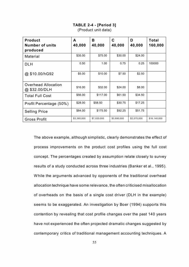
TABLE 2-4 - [Period 3]
(Product unit data)
Product
Number of units
produced
A
40,000
B
40,000
C
40,000
D
40,000
Total
160,000
Material $35.00 $75.00 $30.00 $24.00
DLH
@ $10.00/hG92
0.50 1.00 0.75 0.25 100000
$5.00 $10.00 $7.50 $2.50
Overhead Allocation
@ $32.00/DLH$16.00 $32.00 $24.00 $8.00
Total Full Cost $56.00 $117.00 $61.50 $34.50
Profit Percentage (50%) $28.00 $58.50 $30.75 $17.25
Selling Price $84.00 $175.50 $92.25 $51.75
Gross Profit $3,360,000 $7,020,000 $3,690,000 $2,070,000 $16,140,000
The above example, although simplistic, clearly demonstrates the effect of
process improvements on the product cost profiles using the full cost
concept. The percentages created by assumption relate closely to survey
results of a study conducted across three industries (Banker et al., 1995).
While the arguments advanced by opponents of the traditional overhead
allocation technique have some relevance, the often criticised misallocation
of overheads on the basis of a single cost driver (DLH in the example)
seems to be exaggerated. An investigation by Boer (1994) supports this
contention by revealing that cost profile changes over the past 140 years
have not experienced the often projected dramatic changes suggested by
contemporary critics of traditional management accounting techniques. A
56
1990 Australian survey of manufacturing organisations across 13 different
industry groups revealed that the average product cost profile follows a
55%-20%-25% (material - labour - overhead) profile but varies substantially
across industries captured by the survey.
FIGURE 2-1, Percentage changes of Material, Labour and Overhead costs over 3 periods for
Product A, Products B, C and D show similar trends basis.

57
FIGURE 2-2, Percentage changes of Material, Labour and Overhead costs over 3 periods for
Product A as proportion of the selling price; Products B, C and D show similar trends basis
The example provided in Tables 2-2, 2-3 and 2-4 and illustrated in Figures
2-1 and 2-2 reflects the general status of these findings and confirms the
need to control and allocate overhead costs on a more computational
basis. The more dramatic cost profile change appears to be in the direct
labour and material groupings. As mentioned before both of these
categories have been held constant in relative cost terms over the three
periods but would produce a more dramatic change if these groups
experience increases over the review period. Overhead costs, however,
who had the most significant cost increases during the review period have
only experienced a moderate proportional cost increase. No attempt has

58
been made to identify different activities of the total overhead costs nor to
categorise overhead cost on the basis of cost behaviour into fixed and
variable components.
The benefits derived from such effort would have only a limited impact on
the selling price of the product. In the example, if we calculate the cost
groups as percentages of the selling price then the overhead proportion
reduces to 15.02%, 17.49% and 19.05% for each of the three periods as
illustrated in Figure 2-2. Even if it is possible to identify activities that can
be directly associated with the manufacture of a given product it is unlikely
that this will exceed 50% of the total overhead costs thereby leaving the
remaining 50% again to be allocated on a questionable basis.
Surveys by Anthony and Govindarajan (1983) found that 83% of
organisations use the full cost concept for product pricing of which 50%
used only manufacturing costs, and by Shim and Sudit (1995) found that
70% use full cost pricing, again 50% of those firms that responded relied
on manufacturing costs only for their pricing decisions. This survey
evidence clearly demonstrates the continued reliance on full costs by
organisations in determining their product prices. In the latter survey a third
category (this was not included in the initial survey by Anthony and
Govindarajan (1983) of market-based pricing revealed a 18% application
by responding firms. It can only be conjectured that, if the initial survey had

59
included the market based pricing strategy, the percentage distributions
between full cost pricing, variable cost pricing and market-based pricing
may have revealed a lesser trend reduction in the first two pricing
strategies.
2.1.3 The Variable Cost (or Direct Cost) Concept.
Whereas the full cost concept is based on organisational functions to
distinguish product costs and other organisational expenses, the variable
cost concept distinguishes these cost groups on the basis of cost behaviour
related to the production process. The main classification required to
determine product costs are the identification of variable and fixed cost
groups and assess which specific costs are related to the manufacture and
distribution of goods. As in any of the traditional or emerging cost concepts
there is little disagreement as to the material and direct labour cost
assignments, the arguments relating to achieve improved product cost
accuracy are concerned with the identification and assignment of overhead
costs.
The variable cost concept treats materials and direct labour identical to any
other concept but distinguishes the composition of total overhead costs.
Cost behaviour assumptions are not easily determinable and at times rely
on the experiences of operating personnel rather than verifiable

60
computational data. Fixed overhead costs (e.g. Depreciation, rental,
property taxes, etc.) are not included as product costs but become part of
other operating expenses such as administrative, selling and marketing.
Variable overhead rates which include such cost groups as setup costs,
material handling and quality control are treated as product costs and form
part of the product cost profile. The main difference to any of the data in
Tables 2-2, 2-3 and 2-4 would be changes in the amount of overhead costs
assigned to products. The full cost concept includes all overhead costs in
determining a product’s total cost. The variable cost concept, by only
including the variable overhead cost, will by logic, show a reduced total
product cost with similar trends amongst the cost groups over the three
periods.
In the early 1950s variable costing was popularised and embraced by
management as a better decision tool for product mix decisions because
it provided more accurate product costs based on trend analysis rather than
capacity volume predictions. Most arguments that are advanced against
the usefulness of absorption costing criticise the application of a single cost
driver as the determinant of computing a single overhead application rate.
Variable costing approaches often identify a number of cost pools (or
service departments) and associate appropriate cost drivers with these
cost pools to determine a number of process based overhead application
rates. The same principles can also be applied to the full cost concept.

61
Advantages attributed to the use of variable costs through the distinction
of fixed and variable costs are the ability to compute Cost-Volume-Profit
[CVP] data essential for planning and control management. Other
advantages relate to product cost decisions especially as these are related
to Make versus Buy and special order acceptance. However, the
arguments for or against one of these cost concepts reduces to
insignificance when a period’s production is sold without any inventory
accumulation. As many industries base their production environments on
a continuous improvement philosophy the progress towards zero
inventories is a feasible and likely scenario that would further reduce the
distinction being promoted between full costs and variable costs to a case
of irrelevance. Process improvements, however, will have to be reflected
in product data by providing production reports that present benchmark
levels for performance comparison.
2.1.4 Standard Cost Concept
Each of the two concepts previously discussed rely on past data to identify
the total cost of production and product unit cost profiles. Standard costs
provide a planning foundation that is no longer incorporating production
inefficiencies from past performances but computes product costs based
on current process technologies and labour skills. In additional advantage
derived from the use of standard costing is its ability to provide a base for

62
comparison at different levels of capacity utilisation. While the full cost and
variable costing concepts are useful in determining product costs for
inventory and pricing values, the standard cost concept is applicable to the
evaluation of operational efficiencies and resource consumption. It is based
on the premise that a given resource input must provide a determinable
production output and substantial deviations from this relationship instigate
formal investigations to correct undesirable situations.
The standard cost concept further supports much of the traditional
managerial philosophy of exception reporting. Other advantages that are
attributed to the concept of standard costs are improved cash and inventory
planning, the ability to support responsibility accounting-based
performance evaluation, improved unit cost profiles and incentive schemes
that are tied to predetermined resource consumption. Some disadvantages
have also been identified and include: the interpretation of variances and
the decision rule that initiates process intervention, performance evaluation
tied to incentive schemes are open to manipulation by affected operating
personnel and the concentration of supervisory personnel to minimise
variances may not lead to efficient operational processes as isolated
production sequences are reviewed.
63
Survey results by Gaumnitz and Kollaritsch (1991) and Cohen and
Paquette (1991) indicate a trend in the application of standard costs to
smaller units (departments) regardless of the organisation’s size nor its
industry membership. These results could be interpreted as indicative of
the usefulness of the standard cost concept and that the perceived
advantages provide a greater level of benefits than the cost of the
disadvantages. Although the standard cost concept is an attempt to link
operational efficiencies to accounting data, it suffers the same
shortcomings as the other two cost concepts by relying on an experience-
based allocation of overhead costs.
2.2 The Changing Organisational and Operational Environments.
The example provided (as illustrated in Tables 2-2, 2-3 and 2-4 as well as
Figures 2-1 and 2-2) is based on the assumptions of a product with an
extensive demand history that remained unchanged in functionality and
materials/components used in its manufacture. Manufacturing operations
have benefited from advances in process technologies. The obvious
outcome is found in improved efficiencies that manifest themselves in
producing more output with unchanged or even reduced resources. Labour
intensiveness is being replaced by capital intensiveness. Regional and
global competition has forced many organisations to reassess their
operations to ensure survival and growth.

64
One of the major changes, however, is the shortened product life cycle in
most industries and as a consequence the need to constantly review the
organisation’s product portfolio. This changing environment has also
changed the information need of management away from operational
efficiency management towards strategic management. Product costs as
well as product introductions and abandonment have assumed a major role
in the managerial decision making process. Furthermore, traditional
operational efficiency measures of cost reduction and capacity
improvement without known consumer demand (increase in inventory build-
up) are replaced by an increasing emphasis on quality production,
customer satisfaction and improved throughput times. The latter concept
is also known as manufacturing cycle time or velocity of production
(Garrison and Noreen, 1994:442). The emerging measure of manufacturing
cycle efficiency [MCE] is indicative of the ratio of value-added time to
throughput time. Ratios below 1 indicate that a number of non value adding
activities are still present in the process and could be targeted for
improvement or ultimate elimination.
Managements have identified a number of organisational efficiency
improvements that need to be complemented by appropriate management
information systems. Whereas in the past management accounting
systems have assumed a major role in the information needs of

65
managements, the reduced emphasis on product cost management and an
increasing requirement for non financial performance measures have
depreciated the value of traditional management accounting systems.
Furthermore, a changing emphasis in operational environments from a
traditional capacity utilisation and unit efficiency strategy towards
continuous improvements, zero inventory management, total quality
management and JIT/FMS has created opportunities and demanded
solutions to incorporate these operational strategies into a composite
information system. JIT (Just-in-Time) is an operational philosophy that
relies on known consumer demand (pull demand) to organise material
resource flows, production scheduling and throughput times. FMS (Flexible
Manufacturing Systems) incorporate computer controlled equipment and
scheduling to complement the task of JIT. While there are a substantial
number of related advanced manufacturing technologies [AMTs], within the
context of this argument both JIT and FMS are treated as generic terms for
the changing operational environments embraced by many manufacturing
organisations. Attempts to develop new management accounting and
operations process technologies have found only limited appeal amongst
practitioners.

66
Although there are a substantial number of testimonials in praise of some
of these new system development the lack of a more widespread adoption
of these systems must reflect on their inability to integrate the information
needs of management. Most prominent amongst these new developments
are: ABC (Activity Based Costing), an extension on this theme ABM
(Activity Based Management), Throughput optimisation or ToC (Theory of
Constraints), Total quality Management and the concept of the Lean
Enterprise [LE]. Each of these concepts and their contribution to the
organisational environments will be discussed in the subsequent chapter.
2.2.1 Activity-Based Costing
ABC developed in response to managements needs for more accurate
product costs. Most organisations formulate their pricing strategies on the
basis of their product costs and the shift from labour-based technologies to
machine based technologies without changing the costing algorithm invited
criticism as to the inappropriateness of single cost driver based overhead
allocation techniques.
The popularity of Activity-Based-Costing [ABC] has largely been founded
on the perceived inadequacy of traditional management accounting
techniques which approach the allocation of overheads as a trade-off
between high and low volume production similar to the notion of a modified

67
system of welfare economics. The underlying concept in welfare economics
is based on the work of Pareto, an Italian economist, who discovered that
optimal welfare conditions exist when the benefit given to one group (or
individual) does not affect the benefits of other groups in a negative way.
His discovery has led to the acceptance of the 80/20 rule in which 20% of
one dimension or parameter explain 80% of another dimension. Application
of this rule can be found in quality control analyses, inventory analysis and
cost analysis for various activities.
The allocation of overhead costs on the basis of a single volume-based
denominator level allows the distribution of overhead costs to individual or
product groups in such a way that the allocation of costs to one product has
no negative effect on the product cost profile of another product. By
negative effect, using the concept of welfare economics, it is understood
that a redistribution of overheads does not increase the overhead allocation
of another product thereby reducing its profit contribution. There is an
obligation on system designers to first evaluate if the current allocation
method conforms to the Pareto principle, in deciding to change from the
current system to an alternative system and evaluate if the Pareto condition
has been maintained or violated. A violation may identify those products
that require assessment as to their retention in the current product mix.

68
If we accept this rule in the allocation of overheads by assuming that the
traditional MAS has been developed along the concept of a modified
welfare economics system, it is possible to construct a total overhead curve
on the accumulated distribution of individual product allocations. Such a
model is likely to display close to Pareto effiency conditions as the
overhead allocation is based on changes in volume cost drivers that
attributes equal proportions to all products within the predetermined
allocation algorithm.
With the introduction of ABC-principles into the cost relevance debate it is
of interest to compare the resultant reassessment and re-allocation of
overhead costs based on operational activity analyses with traditional
allocation techniques to ascertain if the changed product cost profiles have
produced a Pareto improvement towards the efficient (optimality) frontier.
Comparisons as presented in most case studies and testimonials are
difficult to reconcile as the ABC cost hierarchy structure of unit, batch,
product and facility costs (activities) incorporate a proportion of period
costs that are not included under traditional MAS and also display
inconsistencies in the treatment and aggregation of direct and indirect
overhead cost behaviours. Other inconsistencies that have been identified
in the application of ABC systems are the arrangement of costpools under
these (4) category headings which creates conflict situations when other

69
operational strategies are pursued and implemented. The Japanese
innovation of a “lean enterprise” [LE] that promotes the concepts of zero
inventories, J-I-T improvement philosophies [that endeavour to achieve
economic production quantities of (1)] and total quality management [TQM]
amongst others finds it difficult to accommodate the activity hierarchy of
ABC.
These apparent conflicts were recently addressed by Cooper (1996) in
which he defends the relevance of ABC even within the lean enterprise
environment by reference to survey results which indicate that
organisations that have adopted lean enterprise concepts have also
implemented ABC. His defence, however, does acknowledge a number of
shortcomings in the area of batch level activities which he feels are
highlighted by an ABC analysis and sensitises management to carefully
consider the difficulties in implementing LE concepts. Although the
criticism about the relevance of ABC system implementations in certain
operational environments is a welcome addition to the debate of problems
faced by contemporary managements, it further directs attention to the
short term emphasis ABC analyses tends to encourage.
The analysis of an organisation’s activities to understand the incidence of
cost incurrence is a helpful first step but is constrained by the rather limited

70
approach of assessing the ability of current practises and existing systems
to affect changes towards “better” product cost profiles. It therefore is
limited to answer questions as to the relevant product cost under current
operational circumstances. ABC, in such case, may be considered by
management as having only a limited appeal for strategic decision making
as it is not addressing issues of consumer choice and production process
capacities. Poorly designed ABC systems also may encourage
dysfunctional behaviour as mis-specified cost drivers (Datar and Gupta,
1994) have the tendency of directing resources towards activities that are
not clearly associated with the prescribed activities. While there is an
acceptance of the general benefit that can be obtained from ABC analysis
its implementation (similar to traditional MAS) relies substantially on
subjective value judgement and consequently subjectively based overhead
allocations.
A substantial body of literature has reported ABC/ABM implementation
successes, reservations about the benefits (Merchant and Shields, 1993)
of implementation and rejections (Bescos and Mendoza, 1995) of ABC
system implementation.
Such inconsistent testimonials must raise doubts as to the perceived
benefits of changing existing information and control systems. Although,

71
ABC techniques have been promoted as necessary tools for management
decision making activities in a turbulent and volatile environment faced by
most organisations, the evidence for general level acceptance and
subsequent implementation by the majority of organisations reviewed in
anglo-saxon countries indicates a general reluctance for such wholesale
acceptance (Drury and Tayles, 1994; Joyce and Blaney, 1990, Dean et al.,
1991; Boer, 1994; Fechner, 1995). The rationality of the ABC concept is
sound and deserves merit for its attempt to redress the perceived
inadequacies of traditional MAS overhead allocation distortions. However,
the level of reluctance to implement an ABC system, after having expanded
a substantial amount of resources on the initial operational analysis raises
the question as to why.
Some of the reasons suggested by a number of authors that are perceived
as disadvantages relate to additional costs of the system and the necessity
to operate two parallel management accounting systems (as the
requirement to provide financial information to external agencies must
conform to GAAP), thereby questioning the real advantages of an ABC
system, especially as it is perceived to be a more complex system with a
remaining substantial amount of non traceable overhead costs (Kaplan,
1994b)

72
To demonstrate this point: let us assume that the untraceable amount of
overheads after having established activities, cost pools and cost drivers
constitutes 40% (facility related) and that the initial overhead were 30% of
product costs (Drury and Tayles, 1994; Joyce and Blaney, 1990, Dean et
al., 1991; Boer, 1994; Fechner, 1995), then the traceable overhead
component is some 18%. Let us further assume that the company's COGS
is 50% of its selling price we, therefore, may have a margin of error
improvement of 9% (30% of 50%=15% and 60% thereof = 9%) of the
selling price. The additional costs to operate and maintain the new ABC
system would further reduce the improvement in accuracy to less then 9%.
Should the company under review operate at substantially greater profit
margins, the benefit from the implementation of a new ABC system
becomes very marginal indeed. Given this very simplistic example,
nevertheless indicates that the benefits from implementing complex ABC
systems are very much dependent on individual companies within industry
groups (Merchant and Shields, 1993).
Kaplan (1994b) has partially addressed this situation by offering an
explanation as to the reason for the difference between ABC distributed
overhead costs and traditional based overhead allocations. He makes the
distinction by pointing out that ABC systems measure the consumption of
resources whereas traditional MAS measures the resources supplied

73
(stewardship function). His admission as to the non traceable portion of
total overheads and his suggestion to reconcile these differences through
the application of variance analysis and subsequent adjustments reinforce
the observed reluctance by many organisations' management to implement
a new management accounting system as the benefits of such a decision
are at best doubtful.
This doubt by management at the individual or group level provides the
background to their resistance to change as the outcome is uncertain.
Argyris and Kaplan (1994) suggest that extensive research evidence has
shown managements concerted efforts in developing defensive strategies
when threatened by new information or theories that question contemporary
management decision models. They support such contention by relying on
prior research that distinguishes between theories-in-use and espoused
theories. Whereas the former describes the rules that individuals use to
guide their actions, the latter contain the values and beliefs individuals
express when questioned (p.94). The espoused theories can be viewed as
analogous to being "politically correct", to use a contemporary term.
A further problem encountered with ABC system design is the number of
activities, cost pools and cost drivers necessary to establish more accurate
and reliable product related data. Amsler et al. (1993) report that their
initial operations analysis of a company's purchasing subfunction generated

74
42 activities and described the difficulty in finding appropriate cost drivers
for these activities especially as the cost objects were not directly
attributable to specific products. They decided that the complexity
generated by the initial analysis was unmanageable and that a compromise
to reduce the 42 activities to a total of six with three cost drivers was
adequate for improving the overhead distribution accuracy. Such
compromise leads to consequences of error incidence at all levels of the
ABC hierarchy, W hile the error at the unit level may have compensatory
and inconsequential effects (due to the lesser weighting at these levels),
error incidence without compensatory effects at the batch, product and
facility level, however, becomes more pronounced. The issue of
diminishing accuracy and increased error incidence caused by the
consolidation of activities and cost pools has received relatively little
attention.
2.2.2 The Theory of Constraints
The basic assumption that underlies the Theory of Constraint [TOC] is that
every operating system must have at least one constraint or bottleneck.
Identifying a bottleneck situation and remedying its effect on the operational
resource flow will generate a production environment of full capacity
utilisation which must lead to optimal profitability. Such approach to
achieving operational efficiency is in direct contrast to efficiency measures

75
motivated by traditional as well as ABC analysis. Many of the techniques
developed by traditional MAS highlight the inefficiencies of localised
resource wastage (e.g. variance analysis) without considering overall
performance. The notion of capacity utilisation is grounded in the belief that
each individual piece of equipment must be utilised to its full capacity (to
avoid the incidence of idle capacity and subsequent unfavourable volume
variances) to achieve optimum operational efficiencies. However,
equipment acquisition and replacement policies rarely, if ever, consider the
effect their installation into an existing operational environment has on the
other components in the process.
Although linear programming and mixed integer programming [MIP] have
become more accessible with the introduction of fairly inexpensive and
powerful computer technology, these techniques are still in the application
range that is used to solve specific problem situations. A more detailed
discussion and application of the [MIP] technique can be found in Kee, R.,
(1995). While the situation presented appears unrealistic as the identified
Constraint is the number of Set-up hours available, it does nevertheless
demonstrate the value of the [MIP] technique. In addition, if sensitivity
analysis is applied to the situation by increasing the set-up hours available,
profit increases. By systematically reducing the newly identified bottlenecks
in the set of constraint equations we will experience a situation where

76
additional resource requirements reduce profitability. It is this condition
which constitutes a point on the Pareto efficiency frontier and is
hypothesized as conforming to the more general 80/20 rule.
However, the mixed integer approach has the additional benefit of
incorporating sensitivity analyses to evaluate the additional costs incurred
in removing the identified bottleneck. Bottleneck mapping and subsequent
improvement will highlight further bottleneck situations so that a
comprehensive analysis can lead to optimal resource utilisation. As each
successive reduction in bottleneck situations will be accommodated by a
cost/benefit profile, overall process improvements can be determined at the
indifference level. The ability of the [MIP] to sequentially evaluate the
benefits from bottleneck reductions will generate a Pareto optimal condition
which is premised on the notion that optimality is attained when a further
improvement in resource inputs leads to a benefit reduction in an output
resource.
Pareto efficiency in the context of this discussion should not be confused
with the concept of Pareto optimality. Pareto optimality is achieved when
the distribution of goods/services falls on the contract curve in a modeled
Edgeworth-Box diagram and represents the condition of optimal
resource/commodity/welfare distribution. The exchange of goods/services

77
beyond a point on the contract curve leads one consumer to be worse off
in his (her) indifference towards a bundle of goods/services. Although the
concept can also be applied to the production possibility frontier
hypothesis, it is not the purpose of this thesis to deal with the economic
rationale of Pareto optimality but instead to introduce the concept of Pareto
efficiency in which a vital few and not the trivial many affect the output
condition of the firm.
While it is appropriate and possible to develop fairly complex mathematical
algorithms to support the notion of Pareto optimality, it is adequate to
accept the application of the [MIP] analysis in establishing a Pareto
efficiency frontier. Pareto Efficiency frontier in the context of this description
refers to the curvature of the accumulated ranked distributions based on
product demand. This demand can be based on trend analysis of past data
or independent predictions of forecasted data. Many situations involving
two-dimensional mappings have found that the Pareto frontier occurs
frequently at the 20%/80% level, the typical 80/20 rule. Examples of this
application and acceptance can be found at quality control investigations,
inventory control modelling (A-B-C model) and of course in its original
social welfare content.

78
Therefore, if we map variables of revenue against product demand
(volume), product diversity against resource consumption, overhead
accumulation against production volume, etc. we may be able to establish
a Pareto frontier for an organisation’s resource consumption which can be
compared with resource consumption profiles of other competitors and in
the ideal situation of the 80/20 condition may provide an independent
benchmark for comparison. Furthermore, by applying the concepts of the
Pareto frontier it should be possible to evaluate the effect of a modification
to an existing overhead allocation system with that achieved by ABC.

79
2.2.3 Strategic Management Accounting
Ward (1992) suggests that strategic management accounting [SMA] could
be thought of as “accounting for strategic management” whereas Bromwich
(1990) subscribes to the view that it is the “provision and analysis of
financial information on the firm’s product markets and competitors costs
and cost structures and the monitoring of the enterprise’s strategies and
those of its competitors in these markets over a number of periods” (p.28).
Strategic management involves the co-ordination of a complex set of
interrelated activities and therefore requires a supporting management
system that can handle the variety of situations and circumstances
confronting the organisation. Ashby’s Law of Requisite Variety, which has
been applied in Cybernetics, “states that it is impossible to manage any set
of variables successfully with a management system less complex than its
variables” (Hosking, 1993) which is supportive of the current movement
towards increased system complexity through the consolidation of existing
but separated discipline dependent system designs.
Management accounting systems that emphasise the necessity to create
an “accurate” product cost profile are likely to confirm Porter’s (1985)
criticism that “while accounting systems do contain useful data for cost
analysis, they often get in the way of strategic cost analysis” (Partridge &
Perren, 1994:22). The usefulness of the ABC technique to analyse and

80
identify the activities that represent the organisation’s value chain and to
determine the appropriate cost drivers for these activities has been rejected
by many practitioners as too complex and by implication too expensive to
maintain. Although many practitioners accept the need for a revised
Management Accounting System [MAS] and concede that ABC provides
a desirable alternative, their reluctance to implement new systems,
however, must reflect on the perceived disadvantages of ABC. In addition
ABC concentrates on internal operational activities that highlight short term
performance and is not well suited to the longer term evaluation emphasis
required by strategic management. Although ABC concepts are suitable to
analyse activities that extend the value chain from supplier to customer,
they seem to lack the decision support features required for market
positioning of the company’s product range.
The development of a clearly defined competitive strategy is vitally
important in sustaining the organisation’s market position and allowing it to
earn superior profits. Porter’s (1985) competitive advantage classification
scheme of cost leadership, focused strategy and product differentiation
provides a basic concept in developing an action plan to achieve such
sustainable advantage. Cost leadership implies that the value adding
activities of the organisation are lower than any of its competitors. Such
advantages can be gained from economies of scale and scope, internally
81
developed technologies and favourable resource acquisition costs that
must be supported by control systems that provide detailed and frequently
issued cost reports to maintain tight cost controls. This is the domain of a
well-designed ABC system. Product differentiation on the other hand
incorporates action plans that position the product in such a way that it is
highly valued and differentiated by customers on a number of desirable
attributes. These attributes may concentrate on customer service,
availability through widely accessible distribution networks, product
reliability and product design (Fechner, 1995:7).
While the concept of competitive advantage provides a focus for
management action plans it needs to be translated into required resource
capacities and acknowledge the constraints that exist within the
organisational resource boundaries. Here again, a well-designed product
cost system is unlikely to reveal operational inefficiencies that are caused
by less well designed process flow systems. To address this shortcoming
we need additional systems that accumulate and analyse data based on
operational efficiencies. ABC systems are not designed to detect poor
product designs as far as manufacturability is concerned nor are the data
gathered relevant to process flow decisions.
The shift from the traditional cost-plus pricing concept to a target based
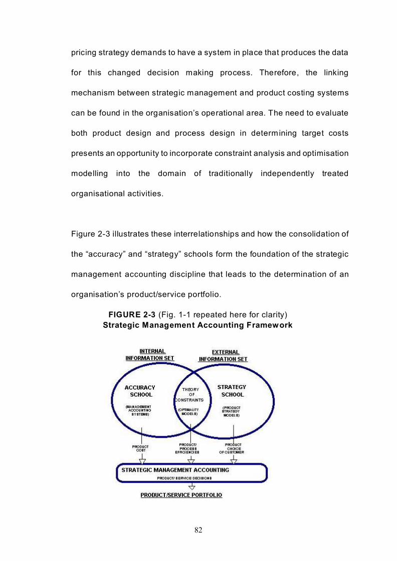
82
pricing strategy demands to have a system in place that produces the data
for this changed decision making process. Therefore, the linking
mechanism between strategic management and product costing systems
can be found in the organisation’s operational area. The need to evaluate
both product design and process design in determining target costs
presents an opportunity to incorporate constraint analysis and optimisation
modelling into the domain of traditionally independently treated
organisational activities.
Figure 2-3 illustrates these interrelationships and how the consolidation of
the “accuracy” and “strategy” schools form the foundation of the strategic
management accounting discipline that leads to the determination of an
organisation’s product/service portfolio.
FIGURE 2-3 (Fig. 1-1 repeated here for clarity)
Strategic Management Accounting Framework

1
The case data has been taken from Cooper & Kaplan (1991) “The Design of Cost Management Systems - T ext, Cases, and
Read ings”, 2nd ED.,Prentice Hall , Englewood Cl if fs, pp.291-310. Al though the sample s ize consist of only 44 components out
of 205 0 tha t con stitute the com pone nt inventory of the com pany, it is neverthele ss a usefu l sam ple to demonstrate some of
the overhead allocation changes under the ABC system design.
83
2.2.3.1 Critical Evaluation of Emerging Management Accounting
Systems
2.2 3.2 Case Study Based Comparison between ABC and MAS.
The following case study of John Deere Component Works [JDCW]1
should provide a good example for the comparison of traditional
MAS versus ABC overhead reassignment. The case study provides
detailed data on overhead costs both direct and indirect, material
weights, component demands, batch numbers and quantity and
actual direct labour hours and costs. The data does not include
material costs nor selling prices. As most of the components are
produced for other entities within the corporation transfer prices are
applied that in most cases do not reflect market traded prices. The
objective of the following data analysis is the evaluation of traditional
MA overhead allocations with the modified overhead allocation by
applying ABC techniques to the same data base.
To repeat the assumptions made for the analysis that follows is the
acceptance that a Pareto efficiency frontier exists for any two-
dimensional mapping within the given data. Furthermore, without
having detailed knowledge of the existing constraints (operational

84
bottlenecks) it is impossible to determine the indifference points
(Pareto optimal condition) for the production (or other functions)
process using the [MIP] technique. It is beyond the scope of this
thesis to apply a detailed [MIP] algorithm to the [JDCW ] data
especially in the absence of known production process constraints.
However, it is acknowledged that the decision to expand resources
to reduce or eliminate operational bottlenecks is a management
decision and may fall short of the optimal condition achievable.
Under these circumstances the optimal condition as determined by
the [MIP] approach can be compared with management’s willingness
to limit resource expansion to compute a profitability variance.
A Pareto frontier is dependent on the overall production process flow
analysis and therefore renders individual component capacity
analysis an ineffectual exercise. To an extent this rather liberal
extension of the Pareto principle to other parameters within the
operational context invites a fair amount of tolerance.
Analysing the data from the [JDCW ] case presents the opportunity
to compare overhead allocations on the basis of the traditional
allocation of standard costs based on departmental rates with the
allocation of overheads on the basis of ABC activity analysis.

85
Figure 2-4 depicts the Pareto frontier of the case data by direct
labour hours (product demand based). It appears that the change to
an ABC system based overhead allocation has made some
difference to the overhead distribution of the products. What is,
however, evident from the illustration is that the lower volume parts
have a reduced overhead allocation under the ABC system. By using
the efficiency frontier mapping the argument often used in favour of
ABC implementations is the notion that traditional allocation
techniques disproportionally undercost low volume products.
FIGURE 2-4
Rareto Frontier,sorted by Direct Labour Hours

86
Although cost data for material and direct labour are not included in
the data (given composite data cannot be reconciled with individual
data groups to insure objectivity within the cost groups) comparison,
it is assumed that the ABC system does not change these cost
patterns. Even under the [TOC] these direct costs are unaffected as
a reduction in bottlenecks will reduce total idle time which is reflected
in indirect overhead costs
.
The question that arises from the above data analysis is twofold.
Firstly, can a limited sample from a given population (2050 parts)
adequately reflect the efficiency parameters and secondly, is it
possible to hypothesise that optimal efficiencies will fall within the
Pareto efficiency frontier. In most case studies relationships are
tested using a number of statistical models (the most popular of
these being regression analysis) to support predetermined
contentions. What is suggested by the Pareto frontier approach is to
accept that a notional benchmark situation exists (80/20 rule) and
through internal adjustments and improvements establish whether
this notional Pareto frontier can be matched. This should not be
construed as an attempt to simply accept that each and every
organisation within a given industry is capable of reaching this
efficiency benchmark but given the ability to apply and assess the

87
outcome of a detailed constraint analysis should contribute to
determine the point of indifference. Expanding resources beyond this
point has the effect of creating a Pareto inferior condition as the
additional resources produce a lesser output.
Figure 2-5 illustrates another interesting relationship in comparing
the overhead allocations between the traditional MAS and ABC. It
appears that approximately 50% of the total overhead costs have
overcosted 13 of the 44 products in the sample and of the remaining
31 products 5 show an extremely high percentage of undercosting.
FIGURE 2-5
Product over/under overhead distribution for the JDCW data

88
These 5 products are all in the low volume category and therefore
are unlikely to have a significant effect on the revenue distribution.
While it is conceded that this type of comparison is less acceptable
to the more traditional comparative approaches offered by statistical
techniques, it does, however, provide an alternative comparison that
should contribute to our understanding of the outcome achievable by
changing overhead allocation techniques.
Rather than relying on the visual presentation for asserting that the
achieved redistribution appears to be insignificant, statistical analysis
is a more acceptable method to test this contention. Using a paired
t-test produced the following results (TABLE 2-5) which partially
confirms the data presented in Figure 2-5. It appears, that the ABC
system has identified some of the period costs as overhead costs
traceable to cost objects (indicated by the negative t-values) and the
subsequent allocation has produced statistically significant
differences between the two systems in direct (variable) and total
overhead costs at the 1% level.

89
TABLE 2-5
Comparison between MAS and ABC
overhead allocations
Variable Correlation t-
value
df 2-tail
Sig.
[MAS] O/H direct 0.948 -3.3 43 0.002
[ABC] O/H direct
[MAS] O/H indirect 0.967 -18 43 0.076
[ABC] O/H indirect
[MAS] O/H Total 0.963 -2.9 43 0.007
[ABC] O/H Total
Interestingly, though, the difference in the allocation of indirect
overheads is not statistically significant between the two systems. It
is difficult to interpret this particular aspect of the analysis as the
case data is taken from a limited sample only. If, however, in
subsequent studies similar results are revealed then the promotion
of “better numbers” or improved accuracy on the basis of indirect
overheads only is more difficult to accept. Naturally, an increase in
sample size or preferably using a company’s total product portfolio
(population) increases the validity of such conjecture.
Further analysis of the data by applying a linear regression model to
ascertain if the initial overhead cost allocation under the traditional
standard cost MAS (that were substantially based on direct labour
costs) may reveal a correlation that explains a lesser variance due

90
to other variables than that achieved by the ABC system. The case
detail describes the use of labour run time as the basis for overhead
computations but provides an example in which labour costs are
used in determining overhead allocation rates. Furthermore, a
change in 1984 from a labour cost base only to a multiple base that
included machine hours and Actual Cycle Time Standard [ACTS]
should affect the direct relationship of DLH/overhead incidence and
be reflected in the data. The results from the regression analysis
reveal that the relationship between DLH and Overhead allocation is
the main predictor of overhead costs. It is therefore surprising to find
that the change over to an ABC system shows an even stronger
relationship between these variables. The case study described a
change in the denominator base prior to the ABC implementation
that included machine hours as well as direct labour costs and Actual
Cycle Time Standard [ACTS] to determine overhead rates. Such
change should be reflected in the coefficient of determination (r2)
when the regression is computed by using direct labour costs as the
independent variable.
Table 2-6 shows the results of the regression with total overhead
(MAS and ABC) as the dependent variables.

91
TABLE 2-6
Regression result of Total Overhead
on Direct Labour Costs
Variable $ t value r2 F
O/H
MAS
37.5 21.25* 0.9 451.49*
O/H
ABC
30.9 25.45* 0.9 647.45*
*p< .0001
Reviewing the results in Table 2-6 shows that ABC allocations are
more correlated with direct Labour costs than MAS allocations.
While this finding does suggest a reversal to single cost pool
overhead allocations, it is nevertheless interesting to note that the
perceived benefit from the implementation of ABC is based on only
6.1% overhead allocation attributable to other parameters. This in
itself is somewhat difficult to interpret as the ABC system
implementation was based on (7) distinct activities and (11) cost
pools. The more likely explanation for these results could be the
inappropriateness of applying OLS techniques to such data and
therefore alternative evaluation techniques are required. Again it
must be stressed that this is a single case study and by its very
nature does not allow any meaningful generalisations. It does,
however, provide an overview of the effects an ABC system has on
the cost profiles of individual products. Amongst the other limitations
92
is the lack of data relating to changes in product demand and the
ability of the production process to cope with the possible changed
demand schedules and the appropriate allocation of production
facilities to suit these changes. Therefore, the evaluation of modified
cost profiles as a result of an ABC implementation must assess the
effect on organisational capacities, both production and
administrative, to ascertain if the additional (or lesser?) consumption
of resources has produced the desired improvement in profitability.
2.2.3.3 Error Incidence and System Accuracy
Datar and Gupta (1994) have made a considerable contribution to
the debate with the development of a quantitative exposition
demonstrating the effect of error incidence on the accuracy of total
product cost profiles. The authors present a quantitative model for
identifying the sources of specification, aggregation and
measurement errors that are a consequence of the complexity in the
design and implementation of an ABC system. The authors further
suggest that the likelihood of an inverse relationship between
specification and aggregation errors on the one hand and
measurement errors on the other hand is an outcome of increased
system complexity. They define:

93
specification errors arise from the choice of cost driver which
does not reflect the demands placed on resources by
individual products, the case study presented by Amsler et al.
(1993:568) provides clear evidence of this situation;
aggregation errors occur when costs are aggregated in single
cost pools although the activities these costs reflect are not
homogeneous. Cost pools that accumulate costs from
heterogenous activities arise when individual products use
different amounts of resources across cost pools, again the
case presented by Amsler et al. (1993:568) provides a good
example;
measurement errors are related to identifying costs within a
particular cost pool and measuring the specific units of
resources consumed by individual products Amsler et al.
(1993:568).
The contention of the Datar and Gupta (1994) paper and others,
(Grunfeld and Griliches, 1960; Lim and Sunder,1990, 1991) is that
the attempt by ABC system designers to reduce the incidence of
specification and aggregation errors (by implementing more activity
specific cost pools and activity specific cost drivers) will increase the
level of measurement errors. The gravity of the measurement error
on the product cost accuracy is a consequence of better specification
and greater disaggregation suggesting that less rather than more
complexity is required for the improvement of overall product cost
accuracy.

94
The authors further suggest that with the incurrence of transaction
and implementation costs, these multiple cost pool systems are
unlikely to capture both diversity and complexity of activities that give
rise to such costs particularly as these and other cost groups cannot
be directly related to cost objects (products).
Therefore, companies should exercise some care during the
analytical stages when identifying and defining cost categories such
as facility related classifications of general and administrative
expenses, rates, taxes, etc. that are difficult to associate with product
specific resource expenditure.
TABLE 2-7
Error Incidence in [ABC] Product Costing Approach
[ABC]
ACTIVITY
LEVEL
COST
DRIVER
COST
POOL
ERROR
INCIDENCE
UNIT determinable specifiable specification
BATCH determinable specifiable aggregation &
measurement
PRODUCT partially
determinable
partially
specifiable
specification,
aggregation &
measurement
FACILITY not-
determinable
difficult to
specify
aggregation &
measurement

95
Table 2-7 provides an overview of the ABC activity levels and the
type of error that is likely to be the consequence of reduced system
complexity. The assumption that the greater the disaggregation of
cost pools and the larger the number of activities identified must
result in greater accuracy of product costs is a misconception and
may help to explain why some of the reported testimonials in various
literature have concluded that the desired outcome, a successful
ABC system implementation, has failed to materialise. The natural
tendency by management to treat new theories and techniques with
healthy skepticism (Argyris and Kaplan, 1994) seems to be partially
supported and justified.
If the proposition of an inverse relationship between complexity of an
ABC system and desired levels of accuracy is accepted, it should be
possible to determine a trade-off value or point of indifference.
However, to determine an optimal level of system complexity some
of the parameters required in the development of such a model must
either be known or must be able to be determined deductively.
Babad and Balachandran (1993) have presented a quantitative
approach to compute an optimal number of cost drivers and an
aggregation of cost pools to determine the trade-off between the cost
of information (transaction recording, data base maintenance, etc.)

96
that evolves as a consequence of complex and detailed ABC system
design and the level of accuracy that produces improved product
cost information. The sacrifice in trading off some accuracy and
therefore an increase in the incident of specification and aggregation
errors should also be balanced against measurement errors.
Finally, the eventual system design should be compared with both
the ABC benchmark (optimal complexity) product costs and the
traditional MAS derived product costs. Only by using the criteria of
error incidence reduction/increase as well as the additional
information related cost incurrence of a fully developed ABC system
does it become feasible to quantitatively compare the cost/benefit
profile of abandoning the existing traditional MAS and implementing
an ABC system on the premise of "more accurate" product cost
information.
The diagramatic presentation depicted in Figure 2-6 adopts the
quantitative details of a relatively simple reported case study
(Pattinson and Arendt, 1994) that limits its analysis to the
disaggregation of a single cost pool of existing overhead costs.
However, this case study (like most other reported testimonials)
suffers from the omission of system related additional transaction

97
and bureaucracy costs which are the by-product of ABC system
implementation and maintenance. Rather then relying solely on a
quantitative comparison of overhead costs established through a
traditional MAS database it proves to be more helpful to provide an
additional graphical analysis that incorporates error variances and
additional system costs on a conceptual basis. The probable cost
behaviour curve for the additional system costs involved in
implementing an ABC system is hypothesised to be linear as the
number of products included is limited to three.
The case study also reports a number of difficulties that were
encountered in establishing the appropriate level of complexity in the
implementation of an ABC system. Although the report analyses a
support function (supply-procurement) of a manufacturing
organisation it reconciles the cost profiles of the traditional MAS with
those of the initially proposed and subsequently accepted modified
ABC system. Such reconciliation is useful as it does not pollute the
original cost estimates or the actual cost reported by the accounting
system.

98
Further, it is of interest to note the reported misgivings by a number
of departments in accepting the complexity of the initially proposed
ABC system, even though it was intended to implement the new
system in the procurement department only. While there was
evidence of resistance to change by most of the departments
involved with the recording of new transactions, estimating the cost
of the new activities and the maintenance of the database,
departmental personnel agreed not to continue with the existing
traditional based MAS and accepted a modified and substantially
aggregated ABC based system.
A common theme of questioning the benefits from the
implementation of the initially proposed system is related to the
additional effort required in supporting the ABC system, the
additional costs and resources that would be incurred and the ability
by manufacturing personnel to manipulate the system in ways that
allowed redistribution of product line costs to other products. The
latter reason (the motivation for cost manipulations provided by the
new system) for the reluctance by departmental personnel to accept
the new system was not evidenced as a disadvantage of the existing
system. The authors offered a number of explanations for the failure
to accept the initial ABC system that can be summarised as follows:

99
- lack of involvement by all departments affected by the new
ABC;
- initial complexity created a resistance towards change and
could have been moderated by a less complex system to be
modified and adjusted after implementation;
S a new ABC system introduced as a better management
accounting system is perceived as not addressing the
performance measures to satisfy the user groups' information
needs;
- the determination of activities and cost drivers must be
complementary across functional support groups.
The case study report also supports the contention of Babad and
Balachandran (1993) that cost pool consolidation has a limited effect
on the numerical accuracy of product cost profiles. The data used in
Table 2-8 is taken directly from the case study and slightly modified
to generate the graphical presentation of Figure 2-6.

100
TABLE 2-8*
(Product data taken from Pattinson and Arendt (1994:61))
Product Product-Charact. Traditional
MAS
ABC-
complex
ABC-
modified
A High Volume $ 10,227.00 $ 5,996.00 $ 6,146.00
B High Vol./Complex $ 8,513.00 $ 6,413.00 $ 6,612.00
C Low Volume $ 2,886.00 $ 9,217.00 $ 8,868.00
MAS set to
zero
Change from
MAS
Change
from MAS
A High Volume $ 0.00 -41.37% -39.90%
B High Vol./Complex $ 0.00 -24.67% -22.33%
C Low Volume $ 0.00 219.37% 207.28%
*for details or numerical example and detail computations refer to Pattinson and Arendt. 1994
The cost curves in Figure 2-6 depict the overhead allocations under
traditional MAS represented by the horizontal line at the zero level
(base line), the initially proposed ABC system (termed here as
benchmark cost curve) and the accepted modified ABC system
(indicated by the modified ABC cost curve). Although the case data
includes only (3) product lines and therefore variances between the
two ABC systems and the traditional MAS are contrasted with this
limitation in mind, the evidence clearly identifies the area of the
aggregation error as defined by Datar and Gupta (1994).The
movement of both under and over costed areas towards the baseline
is logically defensible as the consolidation of cost pools to the
original level of perhaps one used by the traditional MAS would
result in no error variance.

101
FIGURE 2-6
ABC compared to Traditional MAS Product Cost Portfolio
Specification errors are more difficult to identify with only (3) product
lines under consideration but would be expected to increase with the
number of products within the total portfolio. As the number of
products increase it is likely that the intersection point between under
and over allocated overhead costs changes along the horizontal cost
curve of the traditional MAS line thereby shifting the balance of under
and over allocated cost proportion. Predicting the shift of the
intersect is dependent on both product complexity and volume
production, however, intuitively specification errors would increase

102
with product complexity and production process complexity. Such a
proposition requires empirical investigation to test the validity of this
assumption.
Resource consumption for system expenditures in the form of
transaction and bureaucracy costs will have their own economies of
scale and scope and an increase in product numbers will change the
small number product portfolio's linear system costs to a non linear
cost behaviour for larger number product portfolios. .
2.2.3.4 The (IR)Relevance of Cost Management Systems
Differences between MAS and ABC can be attributed to the
treatment of overhead cost allocations. While the traditional MAS
has been criticised on the basis of trade-offs between high and low
volume products by using a single volume based cost driver, ABC,
on the other hand, is based on the identification and analysis of all
activities that contribute to the productive effort and the designation
of appropriate cost drivers for each of these activities to establish a
highly disaggregated overhead contribution matrix that is presented
as a more accurate product costing system. A further assumption
that is promoted as a necessary precondition for the changing of the
cost management system has been the notion of increasing
103
proportions of overheads as proportion of total product costs. This
myth has been dispelled by survey evidence (Whittle, 2000; Boer,
1994) as a generalisation to affect all industries.
Earlier in the discussion the concept of the LE was introduced to
highlight the efforts that are being made to reduce economic batch
production to single digits which, as a logical consequence, would
require an increased number of set-ups for each product. The trade-
off between an increasing number of set-ups per product must be
balanced with the available resources for this function. Here the
assumption is that a reduction in individual set-up times can be offset
with the increased number of set-ups. While this change in
production process strategy is desirable in reducing customer waiting
times, it must also be balanced against the achievement of optimal
profitability.
The example that follows is based on a number of generalised
assumptions that are necessary to provide the analysis. Each of the
four products with its associated data (hours of production
processing) in the example is based on an achievable average
learning curve coefficient and in addition the set-up times are shown
as independent sequential. The latter aspect is of some relevance as
104
in certain situations set-up sequences for certain products may offer
lesser times than for other sequences. For example, if product C is
scheduled to follow product A, set-up times maybe lower than when
product C is scheduled for production after the completion of product
D. Other uncontrollable events such as machine and labour
availability have been considered by using period averages for these
data.
Table 2-9 presents the product data details for (4) products that are
representative of a typical product data information sheet. The
marginal contributions of each product have been calculated (Table
2-9a) using different cost driver selections in each of the three cost
pools (Table 2-9b).

105
TABLE 2-9, Product data*1
*1 Unit cost data has been calculated by dividing the activity cost shown in Table 2-9b for
each of the four products by the respective product demand. Percentage computations
are based on using the unit level ABC costs as base for deviations of all other marginal
and unit overhead calculations.

106
TABLE 2-9a
Product cost and contribution margin data
Notes to Table 2-9a: Inventory details of the company are presented in Case-study 4.3,
p.166. Product data has been modified from original data obtained from
company records. Furthermore, only four products have been selected
to exhibit the difficulties that existed in selecting an appropriate cost
driver for three of the cost pools used by the organisation. The
accumulation of costs in the identified cost pools was established after
some analysis as to homogeneity of these costs. Whereas the cost
pools for set-up and quality control may be classified as batch level
costs, the planning cost pool could include some product level costs.
However, the purpose of the exhibit is to clearly establish that the total
cost in each of the cost pools remains unchanged regardless as to
specification changes of cost drivers. The consequence of such
constant cost pool is that changes in activity costs have no effect on the
total contribution margin. This fact raises the question as to which of the
proposed cost accounting systems provides management with the most
accurate cost. While there maybe an argument for individual product
analysis to establish viability, the optimisation of resources or the
identification of operational constraints remains unaffected by the type
of overhead distribution (allocation) system employed by organisations.

107
TABLE 2-9bCost Pool data using different cost drivers

108
Table 2-10 shows the computation details to calculate different
product costs using a number of different cost drivers. The benchmark
costs have been determined as the most complex, most
disaggregated ABC system in which cost pools contain homogenous
costs and cost driver selection is based on resource consumption by
causal effect. However, as Datar and Gupta (1994) point out, these
costs are difficult to obtain and in most firms remain unobtainable. All
costs included in the cost pools are considered variable in proportion
to the volume produced as any fixed costs that could be attributed to
these cost pools are likely to be treated by cost management systems
as facility level costs (ABC) or period costs (MAS). Furthermore, even
if it would be possible to distribute all overhead costs to cost pools, the
outcome would remain unchanged.
TABLE 2-10
Example (Set-up cost pool) of individual product
activity cost calculations
Product Set-up Turn. Mach. Drill Assy Computations
A x1 y11 y12 ... y1j Product AABC = 3x1 y1j zj
B x2 y21 y22 ... y2j Product BHRS = (3x2 y2j / TH) TC
C . . . . . Product Cno = (x3/ 3xi) TC
D xi yi1 yi2 ... yij
Direct
Labour
Cost
z1 z2 ... zj Total Hours (TH) = 3xi yij
Total Cost (TC) = 3xi yij zj
Also included (refer Figure 2-7) are the traditional MAS allocations
using a single driver (either direct labour hours [DLH] or direct

109
machine hours [DMH]) to demonstrate the level of difference for each
cost driver selection by indicating over or under allocations. The
product data shown in Table 2-9 has been submitted to a constraint
analysis (LP application) to determine the most efficient consumption
of resources given prevailing capacity constraints. The model is based
on the following constraints equations:
TABLE 2- 11
Constraint Equations
Product A B C D Constraint Unit
DLH-ASSY 0.025 0.025 0.025 0.05 <= 8000 Hours
DMH -Turning 0.05 0.05 0.05 <= 8000 Hours
DMH -Machining 0.025 0.1 0.05 <= 10000 Hours
DMH -Drilling 0.025 0.1 0.025 <= 10000 Hours
Batch S ize 1 = 500 Un its
1 = 1000 Un its
1 = 400 Un its
1 = 500 Un its
SET-UPS 1 <= 250
1 <= 250
1 <= 250
1 <= 250
SET-UP (TIME) 1 1 1 1 <= 3500 Hours
QC (TIME) 1 1 1 1 <= 2500 Hours
PLANNING (TIME) 1 1 1 1 <= 3000 Hours
Product Demand 1 >= 0 Un its
1 >= 0 Un its
1 >= 0 Un its
1 >= 0 Un its
Product Margin (ABC) $10.19 $15.54 $14.96 $23.63 =Objec tive Funct ion (max)
The resultant computational values are shown in Table 2-12 also
indicating shadow prices which reflect the benefit (additional profit)
available by relaxing the identified constraints. A further assumption
that underlies the model is that the computed product mix does not
exceed the individual product demand. For example, increasing the
available labour hours in the assembly section would increase the total
contribution margin by $450.00 for each additional labour hour.

110
FIGURE 2-7
Activity Cost Variation[Benchmark - ABC]
The resultant computational values are shown in Table 2-12 also
indicating shadow prices which reflect the benefit (additional profit)
available by relaxing the identified constraints. For example,
increasing the available labour hours in the assembly section would
increase the total contribution margin by $450.00 for each additional
labour hour. A further assumption that underlies the model is that the
computed product mix does not exceed the individual product
demand.

111
TABLE 2- 12
Results report of LP analysis
Solution Cell Starting Final
Total Contribution Margin ($1,010,168.00)$4,209,320.00
Prod. Demand A 1.00 8000 Prod. Demand B 1.00 68000 Prod. Demand C 1.00 60000 Prod. Demand D 1.00 92000
Answer Report Value Constraint Binding? Slack Dual Value
Prod. Demand A 8000 >=0 No 8000.00 0 Prod. Demand B 68000 >=0 No68000.00 0.00 Prod. Demand C 60000 >=0 No60000.00 0.00 Prod. Demand D 92000 >=0 No92000.00 0.00
DLH-ASSY 8000 <=8000 Yes 0.00 450.00 DMH-Turning 8000 <=8000 Yes 0.00 79.00
DMH-Machining 10000.00 <=10000 Yes 0.00 72.00 DMH-Drilling 10000.00 <=10000 Yes 0.00 142
As presented in Table 2-12, the current constraints are concentrated
in all of the production areas suggesting an increase in direct labour
resources through the introduction of a second shift or employment
of additional operators would increase total profitability by the
amounts shown under the dual value column.
Product margin computations have been applied under a number of
different assumptions that include different cost drivers for each of
the defined cost pools. W hile the contribution margins vary
considerably for each of these assumptions (refer to Table 2-9a),
there is no change in optimal profitability. The explanation for such
rather unusual circumstance is based on the fact that the overall cost
within each cost pool remains constant and, therefore, has no effect
on either the capacity constraint calculation or the optimal product
112
mix given the available resources. Furthermore, it supports an
argument for static product mix determinations based on capacity
constraints rather than marginal analysis. In addition, make versus
buy decisions that are also based on marginal analyses and relevant
cost concepts should be reviewed on the basis of product mix
changes and their resultant change in capacity utilisation. Any
analysis based on individual product contribution and subsequent
decision to channel additional resources to the most profitable
product may not result in increased profitability nor is it likely to affect
any of the currently identified constraints. However, what has
become apparent is the limitation any individual product contribution
analysis presents in determining the most appropriate distribution of
available resources.
While the application of the optimisation model was based on
production constraints to determine the optimal product mix (given
a minimum demand for each product to be greater than 0) the model
can be respecified to use product demand as the input variable to
determine the resources required to accommodate that demand. The
model is based on the assumption that the organisation operates as
an entity within a product market where the market demand remains
unaffected by the product supply of the individual organisation. A

113
variation of the model to test for maximum profitability was the
sequential reduction in product demand of one of the four products
to zero (refer Table 2-13). When product A was set at zero overall
profitability increased to $4,216,615 (Alternative 1). All other
permutations produced lower profit amounts when compared to the
initial four product mix solution of $4,209,320 (Alternative 5). The
latter application would complement the strategic-based product mix
choice and focus attention on improving process efficiencies and
capacity optimisation. However, the question as to the most
appropriate product mix choice given the conflicting results of the
product mix permutations (alternative 1 > alternative 5) must be
resolved. Such an impasse can be resolved by reviewing the shadow
prices for each of the solutions and choosing the alternative with the
largest total shadow price (opportunity cost).
TABLE 2-13
Profitability under varying product mix selections.
PRODUCT DEMAND (UNITS)
Alternative Profit A B C D
1 $4,216,615.00 0 70770 58462 95385
2 $2,872,400.00 0 0 80000 80000
3 $3,776,112.00 59250 85188 0 87781
4 $2,641,083.00 69333 37333 90667 0
5 $4,209,320.00 8000 68000 60000 92000

114
By analysing the shadow prices for each of the alternatives as shown
in Table 2-14 and aggregating these prices for each of the
constraints identifies the most desirable alternative. As Table 2-14
demonstrates alternative 1 has a total shadow price of $737 whereas
alternative 5 produces a shadow price of $743 and all other
alternatives contribute substantially below these levels.
TABLE 2-14
Opportunity costs under different product mix constraints.
G137
Altern.
Function
1 2 3 4 5
Resource
Demand
Opport.
COST
Resource
Demand
Opport
.COST
Resource
Demand
Opport.
COST
Resource
Demand
Opport.
COST
Resource
Demand
Opport.
COST
ASSEM BLY 8000 $511 6000 8000 $600 4933 8000 $450
TURNING 7692 8000 $ 580 7352 8000 $ 244 8000 $ 79
M ACHINING 10000 $ 48 4000 10000 $ 70 10000 $ 192 10000 $ 72
DRILLING 10000 $178 10000 $ 40 4324 10000 $ 112 10000 $142
Opport. Cost $737 $ 620 $670 $ 548 $743
While the difference between alternative 1 and 5 is marginal, it is
nevertheless indicative of the most beneficial strategic choice to be
made by the organisation if the overriding objective is considered to
be profit optimisation. The example was based on the assumption
that the organisation’s main objective is the improvement in
shareholder value by offering a product mix that produces optimal
profits. It has been demonstrated (refer to Table 2-9b) that the cost
management system employed is irrelevant in influencing the

115
outcome. Although each alternative has produced different total
costs associated with each cost pool, the overall variable overhead
costs under each cost alternative have remained constant. The
marginal contribution of each product under each of the six cost
management approaches has displayed substantial variation but
does not affect the production process in achieving optimum capacity
utilisation.
The latter outcome is supporting the concepts underlying the TOC. It
is clearly a function of total capacity (resource) utilisation that
determines optimal profitability rather than the idea that marginal cost
analysis or a more accurate cost system leads to improvements in
profitability. Product design and manufacturability are more important
concepts in the determination of optimal profitability and provide
strong evidence that cost accounting systems are largely irrelevant
in achieving this overall objective.
Although the previous example served as demonstration of
emphasising the effect, or lack of effect, on an organisation’s optimal
profitability using a manufacturing organisation’s data, similar
application conclusions can be drawn when the analysis uses a
service organisation to determine profit or service optimality. What
116
changes, however, for service organisations is the definition of
appropriate cost pools as well as defining the level of capacity for
various activities. An initial activity analysis will assist in the
determination of both appropriate cost pools and definable activities.
Furthermore, the case study presentation and analysis in chapter 4
deals with two service type organisations that include a profit oriented
institution (Stock Exchange) and a number of non profit organisations
(various Australian universities). Although, this analysis does not deal
with the specific determination of cost pool identification to compute
capacity optimisation, it is, however, reasonably simple to extend the
previous example to formulate appropriate parameters for these
service organisations.

117
2.3 Chapter Summary
The presentation and discussion together with some critical commentary
on a number of cost accounting techniques have culminated in the
proposition that any of these systems will not influence the organisation’s
optimal profitability. Such proposition is based on the assumption that an
organisation’s product portfolio must be submitted to a resource capacity
optimisation (constraint analysis) rather than relying on individual product
marginal contribution analysis for managerial decision making.
Although the proposition of cost management system indifference is
interesting, the need to develop individual cost profiles remains a
requirement for other organisational obligations. The choice of cost
management system, however, should no longer be considered a
prerequisite for improved profitability.
The continued popularity of simple overhead allocation techniques seems
to support the proposition of indifference. However, the choice of cost
management system may depend on other factors. One of the factors that
must be considered is the accuracy and integrity of the existing data
acquisition system. Data base accuracy is a major concern for any system
that relies on existing and prevailing data to develop prediction models as
aids for managerial decision support systems. Such pre-requisite applies

118
equally well to production based and service organisations. The distinction
in the application between these two groupings must be found in the
identification and determination of relevant model parameters.
The following chapter develops a model that is capable of detecting data
base accuracy and integrity, Furthermore, the model can be applied to
allocate overhead costs on a more relational basis that is complementary
to the organisation’s specified criteria for product cost profiling.
119
3. Model Development.
3.1 Introduction
Although in the previous chapter it was argued that cost management
systems have only limited relevance in determining an organisations
optimal profitability, a cost management system, however, is necessary to
determine profitability in the first place. While the reliance on single volume
cost drivers can produce some distorted cost profiles, its simplicity,
however, seems to be one of its perceived major benefits as evidenced by
a substantial number of survey results (W hittle, 2000) attesting to the
continuing popularity of the absorption cost system. Rather than developing
a complex system of cost aggregations to ascertain a more “accurate”
product cost, it is more likely that organisations will benefit from a less
complex cost distribution system that is based on the organisation’s
production and revenue pattern.
Anecdotal evidence suggests (Koch, 1998) that almost all data bases that
represent the population of data items of interest follow a non linear pattern
when ranked on a two dimensional criteria. What’s more the pattern often
identified follows the Pareto principle or the 80/20 rule. This generalised
distribution has been popularised in 1950 by Joseph Juran who observed
that in many applications the vital few, not the trivial many, accounted for
the majority of problems related to quality of output. Since then the Pareto

120
principle has often been referred to as the 80/20 rule or A-B-C analysis (or
classification). A well known application of the A-B-C classification within
the accounting domain has been in inventory control system design.
Identifying products on the basis of their individual value in relation to the
total value of inventories provides a sound approach for determining the
resources to be expanded in controlling a major asset in most
organisations. An extension to this product classification as to the individual
product value within the total product portfolio would be to analyse if the
product cost profiles follow a similar distribution with particular emphasis
on the overhead proportion. While it is hypothesised that the resource
consumption of products parallels this of the inventory classification
ranking, normal statistical analysis should support such conjecture.
However, the simple ranking of data base items to confirm the existence of
a Pareto distribution that displays a cumulative upward sloping curve
provides limited benefits for predictive computations of the variables
selected.
To utilise the identified Pareto curve or Pareto frontier, the development of
a model that mirrors the Pareto frontier of a given data base would provide
the computational foundation to calculate point estimates that are
consistent with the Pareto frontier. The Generalised Pareto Distribution
(GPD) was first introduced by Pickands (1975) and has the following
distribution function:

121
...................................(1)
where a = positive scale parameter
k = shape parameter
the density function for the GPD is:
.......................................(2)
where a and k are as before the scale and shape parameters. This model
is often applied to compute values for extreme distributions in both the fat
and long tail to predict future occurrences of interest. To utilise the GPD
both parameters a and k need to be calculated by reference to the
underlying data sample. It is obvious that the computation of these
parameters is critical for the predictive ability of the model but is limited to
point rather than incremental value estimates.
Extensive literature research did not reveal the existence of a model that
incorporates the characteristics necessary for the prediction of variables of
interest. Mathematical modeling of data base patterns constitutes the
primary step in the model development, followed by statistically testing the
“real” data base pattern against the model generated values. Rather than
relying on the extensive anecdotal evidence provided and discussed by
Koch (1998), data analysis approaches of random number generated data

122
bases as well as publicly available data bases will be investigated to
establish a consistent data item pattern that produces a Pareto frontier.
A further benefit expected from the data base analysis strategy is a
consistent pattern or Pareto frontier over a number of periods within the
investigated domain. Although anecdotal evidence is not available to
support this proposition, inductive reasoning from many case study details
presented by Koch (1998) would strongly support such hypothesis. Should
this phenomena prove to be correct then the model can also be applied to
identify data base inconsistencies that are caused by recording errors or
omissions of data item details.
3.1.1. Database Integrity
While literature in general acknowledges the existence of data base errors
(Valenstein and Meier, 1999) through faulty recording as well as detail
omissions, there seems to be limited empirical evidence to support this. It
also appears that most of the studies concerned with error entries is
reported in the general medical and associated literature. The concern
amongst medical professionals is often related to the treatment and test
ordering of patients as any erroneous record could lead to eventual
litigation. Some additional evidence is provided by Grasha and Schell
(2001) in an experimental setting to test the incidence of error entry and

123
product selection errors by a group of undergraduate students of mixed
gender. The presumption made by these researchers is the general modal
rate of error incidence of between 3% and 5% in the pharmaceutical
domain of prescriptions filled. However, Grasha and Schell (2001:53) claim
that “Sequential, self-paced, repetitive tasks whereon the output of one part
serves the input for the next component are very common.” and list a
number of examples including the filling of warehouse orders. The filling of
warehouse orders has a number of distinct sequential tasks starting with
the acceptance of the order either through verbal communications
(telephone acceptance) or electronic based entries (e.g. web based) and
completing the cycle by picking the items and shipping them. Data entry is
mostly via keyboard into the local inventory data base from which a picking
slip is produced to initiate the order picking and subsequent shipping cycle.
At each of these sequential data entry and item picking steps error
incidence will occur at lesser or greater levels depending on the internal
control systems employed by the organisation.
Surprisingly, there is very little literature in the auditing arena devoting
empirical research to data base integrity, although similar consequences
as those anticipated by the medical profession could be anticipated by the
auditing profession. However, one reason for the paucity in data base
integrity research within the auditing domain maybe the regulated ability to

124
declare detected deviations in recorded data only if these deviations
exceed materiality limits. In many cases the materiality concept requires
deviation reporting if the differences in recorded data varies by more than
10% from factual situations. A good example are inventory record
deviations from physical counts.
In subsequent sections of this chapter the basic framework for the Pareto
frontier model is presented, the results of the developed model’s generated
values against both the random number generated data bases as well as
the publicly available data bases are statistically evaluated to confirm both
pattern consistencies and model robustness. An additional advantage of
using computer generated data bases is the avoidance of entry as well as
omission errors. The final section will discuss some of the limitations of the
model as a predictor of future pattern analysis.

125
3.2 Development of A Pareto Frontier Model.
The characteristic of the Pareto distribution clearly represents a non-linear
relationship between two variables of interest. As such, models like the
general decay/growth model, the learning curve model, the economic
average total cost curve model, as well as the GPD model as shown in
equation (1), serve as a good starting point for the development of a Pareto
(Pareto frontier) model. W hile the GPD model incorporates both shape and
scale parameters, the computations are concerned with point estimates of
data elements at the long and fat tail regions of the distribution. Such
limitation is too restrictive for the current research question and a more
relevant starting point for the development of the model criteria can be
found in the typical form of a negatively sloping exponential model that is
presented in the following functional relationship:
In addition, the model must meet some specific relational criteria between
variables one and two. The question that arises, however, concerns the
validity of developing a model for the computation of point estimates of an
existing data base that provides an accurate representation of the
distribution of the individual elements. While it may be inappropriate to
employ a model for the calculation of individual item contribution to verify

126
an unbalanced distribution, when it concerns the verification of overhead
cost allocation, the need for comparing an existing allocation against an
impartial benchmark is justified. The reason for the latter argument can be
found in many practical applications where initial recording of prime cost
items produce substantial variances against a preset standard. The
traditional management accounting system has been criticised because it
allocates overheads on a single cost driver based volume approach which
leads to prime cost variations that are likely to amplify the misallocation
problem.
Most Pareto based modeling is accomplished by analysing data bases to
establish distributional characteristics that complement a desirable
criterion. These evaluations rely on access to data bases that represent the
total population of elements of interest. An example of such approach is the
ranking of inventory items on the basis of total item value in descending
order. Such approach can be denoted as x1$x2$x3.......$xn. Coordinate
pairs (xi,yi) are then computed by equation (4). Simple cumulative
calculation of individual item proportion being added to preceding items
within the sequence will produce an upward sloping continuous (without
inflection points) curve starting at the origin (0%, 0%) and terminating at the
terminal data pair (100%, 100%). The general form of a cumulative model
is shown below::

127
where yi cum = cumulative percentage of the i th item in the data basexi = ith individual item
n = total population of data base
The first term on the right hand side computes the item’s individual
percentage contribution while the second term represents the cumulative
value of all items preceding the ith item. To accomplish the analysis of
population data bases, standard spreadsheet applications can be utilised
to establ ish an initial computational data array that consists of the
parameters required to compute item contributions that mirror a typical
Pareto or unbalanced distribution.
Three (3) pre-determined data points must fall on the aggregated data
curve which are the origin (0%, 0%), the reference criterion (20%, 80%) and
the terminal value (100%, 100%). Although the initial or origin of the Pareto
distribution is constituted by the this point estimate, the first data pair (x1,y1)
however, is the point estimate of origin and becomes part of the modeling
process to determine the model parameters. The initial model developed
takes the following form:

2The ? In the 20/? refers to a parameter choice in the i terat ion process as the assumption of a third undetermined focal
poin t on the pare to fron tier c ann ot be ass um ed to be c ons istently at the 8 0% level on the y axis.
128
where a = constant term (obtained through iteration process given PT)PT = total number of products in portfolioxi = ith product rank within portfolioyi cum = cumulative percentage of ith product contribution
Again, note as commented for (4), the first term on the right hand side
computes the product’s individual percentage contribution while the second
term represents the cumulative value of all products preceding the ith
product.
While the Pareto model depicted in (5) allowed computations to determine
the focal 20/80 data point it was, however, more difficult to determine the
value for the very first data pair in a given data base. As the main purpose
of the model is to provide a standard Pareto frontier that allows item
comparison of an existing data base, it is necessary to specify both the
(20/?)2 data pair as well as the first item contribution. The terminal
(100%/100%) data pair is a consequence of the common denominator
which by the logic of the equation will always be unity. Testing of the model
against a variety of different generated data bases revealed a weakness

3
For a m ore detailed discuss ion on W eibull distribu tions refer to Duf fy, S .F., and Baker, E .H., “W eibull Param eter
Es timation - Theory and B ackground Inform ation”, http:// www.csuohio. edu/civileng/ facu lty/ duffy / Weibull
_Theory.pdf pp. 1-22.
4
Notation of the base for the natural logarithm varies from exp to (e) only. This thesis adopts the convention of
abbreviated descriptor.
129
that produced inconsistent values for the first item contribution when the
constraint was equated to the value of the first item in the “real” data base.
To overcome the model’s inconsistency (lack of robustness under changing
parameters) a more robust model development was necessary. Although
a number of sample inventory data bases from a current research site were
used for model mapping and item comparison, the relatively small number
of these data bases (inventory records for 7 years) was insufficient to
provide the necessary confidence level for the general model. The original
data bases were used as input data in a curve fitting software application
to establish the best fit of the non linear characteristics of the data base.
The W eibull3 model consistently produced the best fit with the highest
correlation coefficient and the lowest error term. The standard Weibull
model consist of the following terms:
where a,b,c and d = are parameters that are calculated and become constants fora given data base.
e4 = base of Napierian or natural logarithm (2.718281)
While the Weibull model mimics the curvature of a typical Pareto

5
T he model shown here was developed through extensive use of Spreadsheet based optimisation functions and
automated macro applications. W hile these are obtainable from the author, they are still in a developmental stage
and w ill be incorporated into a functional software package in the near fu ture.
130
distribution it has only limited robustness in computing point estimates.
Furthermore, the computed point estimates must be aggregated to
establish a cumulative distribution presentation. Through continuous
iterations of the unknown parameters (initially they set at 1) values for each
of these are ascertained. Experimentation with the basic model
(mathematical modelling process) and inclusion of the base variable
metrics (x) produced the following model5:
where P = total number of products in portfolioxi = ith product rank within portfolioyi cum = cumulative percentage of ith product contributionc = constant for a given data base.(xi/P)d = term that determines the shape parametere = base of natural logarithm (2.718281)
As the Weibull model is normally applied to failure data (materials) and
therefore has a minimum data pair, the inclusion of a constant term (a or ")
is necessary for the prediction of material characteristics. Furthermore,
such a prediction model, similar to ordinary linear regression models,
analyses sample data to infer characteristics or attributes of the population.

131
To apply Pareto analysis to a data base, however, is based on the data
availability of a population. Therefore, as both initial and terminal data pair
values are known, the inclusion of a constant term representing the
intercept at the lower limit of the relevant range is irrelevant. The main
purpose of the model (5, 7) is to calculate point estimates for any item
within the data base and compare it with the curvature of the actual
distribution. The assumption made to defend this proposition is based on
the model’s ability to mirror the data points of the original distribution with
minimal deviation and the proviso that a data base comparison between the
“real” random data base and the model computed data base reveals
statistical insignificance. If the statistical analysis confirms this proposition
then the model can be applied to organisational data bases to reveal any
inconsistencies in the allocation of overhead costs and thereby alert
management to these inconsistencies for further investigation. In addition
overhead cost adjustments for product deletions or product additions can
be established through the application of the model.
Traditional cost accounting systems simply apply the cost driver (e.g. direct
labour hours) to determine the level of overhead allocation to a new
product, whereas the deletion of a product without an offset in capacity
demand will distribute the allocated overheads from the deleted product to
all other products on a resource consumption basis. The underlying

6
Data bases were c reated with the aid of the random num ber generator function found in most spreads heet
application. The author used Corel Quattro Pro for the generation of the data bases.
132
assumption for such re-distribution of overhead costs is based on the
premise that demand and costs behave in a linear relationship. This
assumption is evidenced in most management accounting textbooks where
the determination of overhead predictions follows the application of
simplistic linear regression models (Horngren et al, 1994, 1996).
3.3 Data Base Generation and Pattern Recognition
The development of the model (7) required the analysis of a number of data
bases with varying numbers of elements and varying parameter
assumptions. During this process data bases with total element numbers
of 500, 1000, 2500 and 4000 were created randomly6 together with
parameters that represented product demand, price and shape factor. For
each of these populations 800 data bases were created. In addition, for
each random generated data base a model computed database was
produced to provide a comparison between the parallel bases. The final
number of generated data bases amounted to 6400 ( 800 for each 500 item
level, 1000 item level, 2500 item level and for the 4000 item level - and the
same number for each of these item numbers through the computed data
base). The metrics for price level was varied between $0.01 and $10.00
and between $0.01 and $100. Demand metrics were varied between 1 and
5000 and 1 and 10000 items.

133
The initial number of generated data bases using the “uniform” distribution
function produced consistent distributions at the(20/50) level. While this
outcome was of only minor concern to test the developed model it did not,
however, mirror the reported empirics (Koch, 1998). In order to generate
data bases that reflect the (20/80) distribution a shape factor was
introduced and varied at the upper ranges. The shape factor was randomly
varied between 1 and 1.4 in the first hundred data bases for each
population and between 1 and 1.45 for the second hundred data bases. For
all the items data bases the shape factor was held constant for changes in
price and demand. The permutations for each of the selected item data
bases were as follows:
Price range Demand range Shape factor
Data base 1 $0.01 - $10 1 - 5000 1 - 1.4Data base 2 $0.01 - $10 1 - 5000 1 - 1.45Data base 3 $0.01 - $10 1 - 10000 1 - 1.4Data base 4 $0.01 - $10 1 - 10000 1 - 1.45Data base 5 $0.01 - $100 1 - 5000 1 - 1.4Data base 6 $0.01 - $100 1 - 5000 1 - 1.45Data base 7 $0.01 - $100 1 - 10000 1 - 1.4Data base 8 $0.01 - $100 1 - 10000 1 - 1.45
All of the 3200 data bases were submitted to standard statistical analysis
(ANOVA) to determine within group and between group differences and were
found to be statistically similar as evidenced by the following tables (Table 3-1 -
Table 3-4). The model generated data bases produced similar non significant
results for differences between the “real” random data base and the parallel

7
The com plete data for all data bas e values are available from the author on request. As the main purpose of the
modelling process was the generation and testing of error free data bases, the inclusion of the s tatist ical analysis
of the model generated data bases are not relevant to this process.
134
model data base for the same 3200 data bases.7 However, each “real” data base
was submitted to a standard ANOVA test against its parallel “model” data base
to determine that the error term was within the level of insignificance. There was
no single case in which the F value exceeded the critical F value for each of the
3200 cases and it can therefore be stated with confidence that the model is
robust within the 95% confidence level that formed the basis for all ANOVA tests.

135
TABLE 3-1
Results of ANOVA for data distribution of 8 (500 items) data bases
Data 500 Price $ Demand # Shape F.(^2) ANOVA(Source of Variation) SS df M S F P-value F crit
1-10 1-5000 1-1.45 Between Groups 2.74 99 0.028 0.743 0.974 1.245
W ithin Groups 1857.47 49900 0.037
Total 1860.21 49999
1-10 1-5000 1-1.4 Between Groups 2.37 99 0.024 0.589 1.000 1.245
W ithin Groups 2029.29 49900 0.041
Total 2031.67 49999
1-10 1-10000 1-1.45 Between Groups 2.38 99 0.024 0.673 0.995 1.245
W ithin Groups 1780.57 49900 0.036
Total 1782.95 49999
1-10 1-10000 1-1.4 Between Groups 2.56 99 0.026 0.660 0.996 1.245
W ithin Groups 1956.84 49900 0.039
Total 1959.40 49999
1-100 1-5000 1-1.45 Between Groups 2.12 99 0.021 0.667 0.996 1.245
W ithin Groups 1598.44 49900 0.032
Total 1600.56 49999
1-100 1-5000 1-1.4 Between Groups 2.45 99 0.025 0.690 0.992 1.245
W ithin Groups 1788.47 49900 0.036
Total 1790.92 49999
1-100 1-10000 1-1.45 Between Groups 2.24 99 0.023 0.723 0.983 1.245
W ithin Groups 1560.17 49900 0.031
Total 1562.40 49999
1-100 1-10000 1-1.4 Between Groups 2.37 99 0.024 0.693 0.991 1.245
W ithin Groups 1725.98 49900 0.035
Total 1728.35 49999
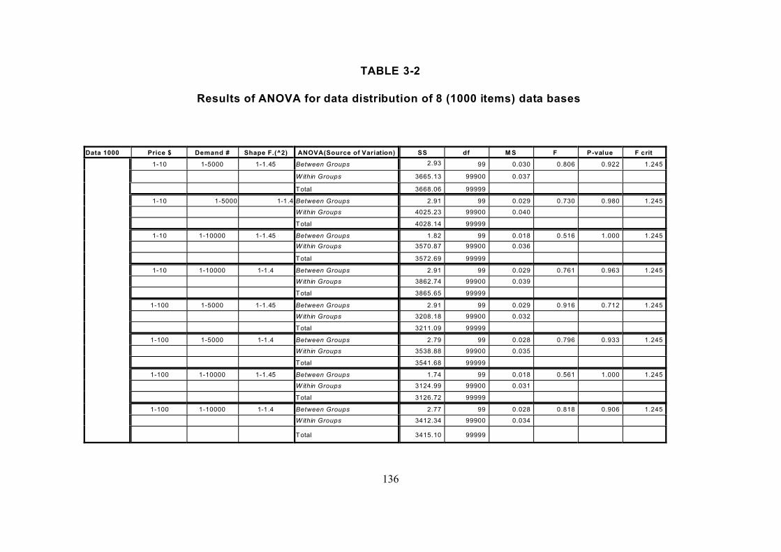
136
TABLE 3-2
Results of ANOVA for data distribution of 8 (1000 items) data bases
Data 1000 Price $ Demand # Shape F.(^2) ANOVA(Source of Variation) SS df M S F P-value F crit
1-10 1-5000 1-1.45 Between Groups 2.93 99 0.030 0.806 0.922 1.245
W ithin Groups 3665.13 99900 0.037
Total 3668.06 99999
1-10 1-5000 1-1.4 Between Groups 2.91 99 0.029 0.730 0.980 1.245
W ithin Groups 4025.23 99900 0.040
Total 4028.14 99999
1-10 1-10000 1-1.45 Between Groups 1.82 99 0.018 0.516 1.000 1.245
W ithin Groups 3570.87 99900 0.036
Total 3572.69 99999
1-10 1-10000 1-1.4 Between Groups 2.91 99 0.029 0.761 0.963 1.245
W ithin Groups 3862.74 99900 0.039
Total 3865.65 99999
1-100 1-5000 1-1.45 Between Groups 2.91 99 0.029 0.916 0.712 1.245
W ithin Groups 3208.18 99900 0.032
Total 3211.09 99999
1-100 1-5000 1-1.4 Between Groups 2.79 99 0.028 0.796 0.933 1.245
W ithin Groups 3538.88 99900 0.035
Total 3541.68 99999
1-100 1-10000 1-1.45 Between Groups 1.74 99 0.018 0.561 1.000 1.245
W ithin Groups 3124.99 99900 0.031
Total 3126.72 99999
1-100 1-10000 1-1.4 Between Groups 2.77 99 0.028 0.818 0.906 1.245
W ithin Groups 3412.34 99900 0.034
Total 3415.10 99999

137
TABLE 3-3
Results of ANOVA for data distribution of 8 (2500 items) data bases
Data 2500 Price $ Demand # Shape F.(^2) ANOVA(Source of Variation) SS df M S F P-value F crit
1-10 1-5000 1-1.45 Between Groups 1.88 99 0.019 0.513 1.000 1.245
W ithin Groups 9261.28 249900 0.037
Total 9263.16 249999
1-10 1-5000 1-1.4 Between Groups 2.34 99 0.024 0.585 1.000 1.245
W ithin Groups 10083.78 249900 0.040
Total 10086.12 249999
1-10 1-10000 1-1.45 Between Groups 2.32 99 0.023 0.662 0.996 1.245
W ithin Groups 8835.62 249900 0.035
Total 8837.94 249999
1-10 1-10000 1-1.4 Between Groups 1.86 99 0.019 0.481 1.000 1.245
W ithin Groups 9730.35 249900 0.039
Total 9732.20 249999
1-100 1-5000 1-1.45 Between Groups 2.05 99 0.021 0.644 0.998 1.245
W ithin Groups 8027.21 249900 0.032
Total 8029.26 249999
1-100 1-5000 1-1.4 Between Groups 1.79 99 0.018 0.506 1.000 1.245
W ithin Groups 8916.52 249900 0.036
Total 8918.31 249999
1-100 1-10000 1-1.45 Between Groups 1.63 99 0.016 0.529 1.000 1.245
W ithin Groups 7785.79 249900 0.031
Total 7787.42 249999
1-100 1-10000 1-1.4 Between Groups 1.71 99 0.017 0.503 1.000 1.245
W ithin Groups 8602.38 249900 0.034
Total 8604.09 249999

138
TABLE 3-4
Results of ANOVA for data distribution of 8 (4000 items) data bases
Data 4000 Price $ Demand # Shape F.(^2) ANOVA(Source of Variation) SS df M S F P-value F crit
1-10 1-5000 1-1.45 Between Groups 1.93 99 0.019 0.527 1.000 1.245
W ithin Groups 14799.72 399900 0.037
Total 14801.65 399999
1-10 1-5000 1-1.4 Between Groups 2.42 99 0.024 0.660 0.996 1.245
W ithin Groups 14793.63 399900 0.037
Total 14796.04 399999
1-10 1-10000 1-1.45 Between Groups 2.63 99 0.027 0.747 0.972 1.245
W ithin Groups 14188.00 399900 0.035
Total 14190.62 399999
1-10 1-10000 1-1.4 Between Groups 2.53 99 0.026 0.658 0.997 1.245
W ithin Groups 15550.27 399900 0.039
Total 15552.80 399999
1-100 1-5000 1-1.45 Between Groups 1.78 99 0.018 0.557 1.000 1.245
W ithin Groups 12907.86 399900 0.032
Total 12909.64 399999
1-100 1-5000 1-1.4 Between Groups 1.86 99 0.019 0.526 1.000 1.245
W ithin Groups 14248.95 399900 0.036
Total 14250.81 399999
1-100 1-10000 1-1.45 Between Groups 1.74 99 0.018 0.565 1.000 1.245
W ithin Groups 12420.98 399900 0.031
Total 12422.72 399999
1-100 1-10000 1-1.4 Between Groups 1.82 99 0.018 0.534 1.000 1.245
W ithin Groups 13743.32 399900 0.034
Total 13745.14 399999

139
To reduce the limitation of subjectively choosing the 20% focal point of the
(x) dimension, a stratified selection of the random generated data bases
were used and additional focal points (x values) at the 10%, 30%, 40%,
50%, 60% and 70% level were submitted to analysis to determine
variations in error levels. The range of error terms at any of these levels
remained within the original range (refer Table 3.5) at the 20% level. This
analysis clearly established the validity and robustness of the model and
justified the subjective choice of the 20% level as it is representative of the
20/80 rule discussed in other literature (Koch, 1998). A further comment on
the use of a model that mirrors the original data base is its variation at the
point estimates. These point estimates are useful to establish domain
pattern similarities and also provide the basis for comparison between
original data base and model generated data base. However, this function
is limited to verify the integrity of an existing data base and identify the level
of variation for further detailed investigation. A more important function of
the model however, is the ability to compute item contributions within the
cumulative framework. For this reason it is important to analyse and
compare the differences in item contribution rather then the item’s point
estimate.
Point estimates compare the cumulative percentage between “real” and
model data base values which, given the argument provided earlier as to

140
the likelihood and risk of data base inaccuracy due to error entry and data
omission would render such comparison as meaningless and therefore the
associated error term would not be indicative of the robustness of the
model. Table 3-5 shows the analysis of this pairwise comparison for each
of the 3200 data bases with average, maximun and minimum values for
both the incremental and point estimate values.
Error term analysis is absolutely necessary to establish the robustness of
the model under varying parameters and to calculate an upper and lower
boundary that can be applied to predictive data. For each of the random
generated data bases the standard statistical parameters for populations
(mean, variance and standard deviation) were recorded to establish the
range of values over the 3200 data bases used in the modeling process.
The standard notation for the mean, variance and standard deviation can
be found in any introductory statistics text but is shown below for
completeness.
Mean
Variance
Standard Deviation

141
Table 3.5 shows the values of these parameters. Here the argument could
be advanced that the maximum and minimum values from the 3200 data
bases are a better indication of the confidence interval limits than the
calculation of the confidence interval at the 95% level. However, for
completeness and accepted practice the confidence interval for the data
presented in Table 3-5 is computed as:
Table 3.5
Error data for incremental and point differences
INCREMENTPOINT
µ F2F µ F2
F
-0.00001% 0.00002% 0.04203% Mean-N 500 -0.42661% 0.00863% 0.83094%
-0.02074% 0.00006% 0.06036% Mean-N 1000 -0.40267% 0.00964% 0.87698%
0.00001% 0.00000% 0.00653% Mean-N 2500 -0.40291% 0.01586% 1.10361%
-0.00004% 0.00000% 0.00395% Mean-N 4000 -0.40267% 0.00831% 0.87421%
-0.00000% 0.00017% 0.13131% Max-N 500 0.09425% 0.03186% 1.78503%
-0.00042% 0.00038% 0.19420% Max-N 1000 0.02365% 0.08939% 2.98974%
0.00021% 0.00000% 0.01494% Max-N 2500 -0.03714% 0.12288% 3.50549%
-0.00000% 0.00000% 0.00900% Max-N 4000 -0.01889% 0.02293% 1.51419%
-0.00003% 0.00000% 0.01540% Min-N 500 -1.29750% 0.00045% 0.21124%
-0.07956% 0.00000% 0.00893% Min-N 1000 -1.01633% 0.00044% 0.21089%
-0.00029% 0.00000% 0.00266% Min-N 2500 -0.83952% 0.00034% 0.18461%
-0.00040% 0.00000% 0.00124% Min-N 4000 -0.76804% 0.00025% 0.15828%
Note: Subscripts D and M identify “real” data base and generated model data base item values.
The confidence interval for the incremental data with a maximum F (refer
Table 3.5) = .1942%(±1.96) = ±.380632% and maximum : (refer Table 3.5)

142
= .00021%x(±.380632%) thereby creates a confidence interval with a lower
boundary of -.3804 and an upper boundary of +.3808. While the point
estimate has little relevance for the computation of predictive data (e.g.
overhead) it shows a substantially greater confidence interval then the
incremental error term. For completeness and using the same values as for
the incremental value the point estimate interval is for the maximum F (refer
Table 3.5) = 3.505%(±1.96) = ±6.87% and a maximum : (refer Table 3.5)
= .0904%x(±6.87%) = -6.78% and +6.96%.
The general shape of one of those (2500 element population) random
created data bases together with its computed model (7) values are shown
in Figure 3-1.
FIGURE 3-1
Data Base and Model Comparison

143
Figure 3-2 illustrates the error distribution of the data comparison for
differences between the individual increment at each point estimate. The
error distribution illustrated in Figure 3-2 shows an overall distribution range
from + .067% to -.051% which is atypical for most of the compared data
bases.
FIGURE 3-2
Typical Incremental Error Distribution
While this error distribution shows a minimal amount of variation at each of
the incremental point estimates, it does not reveal the variation or standard
deviation of the error term to construct a meaningful confidence interval.
W e are assisted by a standard summary measure for population data sets
and do not have to rely on estimates of the main parameters of interest.

144
Having established the basic parameters for the population it is now
possible to construct appropriate confidence intervals. It is often desirable
to first decide on a confidence coefficient that allows the construction of the
range of the confidence interval. The confidence coefficient is commonly
expressed as a percentage and having decided in the earlier ANOVA
computations to use an alpha level (") of .05 it is consistent with this level
to establish a confidence coefficient of .95 or 95%.
Such interval determines that the calculated point estimate of a population
will have an upper and lower limit and that the calculated value will, with a
95% confidence level, be an accurate prediction of the value computed.
The parameters for the random generated database represented in Figure
3-1, 3-2 and 3-3 have been computed to have a mean of the incremental
value differences of 0.00, a variance of 0.000 and a standard deviation of
0.0001%. These values would construct a confidence interval which at the
95% as well as the 99% confidence coefficient becomes equal to the point
estimate at the predicted value. A more probing test would have to
consider the differences in point values between the random generated
data base and the model computed values. This error distribution is
presented in Figure 3-3 and shows a more discernable error distribution,
the values calculated for the error distribution shown in Figure 3-3 are as
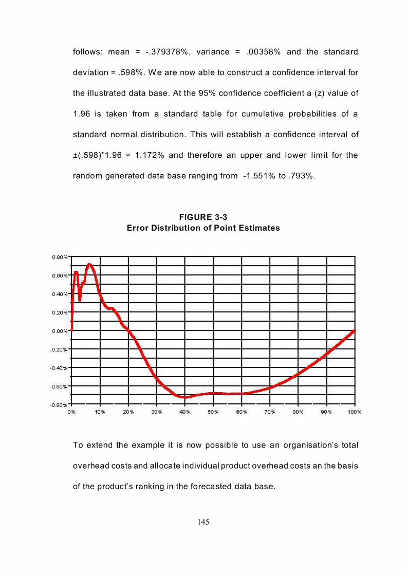
145
follows: mean = -.379378%, variance = .00358% and the standard
deviation = .598%. We are now able to construct a confidence interval for
the illustrated data base. At the 95% confidence coefficient a (z) value of
1.96 is taken from a standard table for cumulative probabilities of a
standard normal distribution. This will establish a confidence interval of
±(.598)*1.96 = 1.172% and therefore an upper and lower limit for the
random generated data base ranging from -1.551% to .793%.
FIGURE 3-3
Error Distribution of Point Estimates
To extend the example it is now possible to use an organisation’s total
overhead costs and allocate individual product overhead costs an the basis
of the product’s ranking in the forecasted data base.

146
Product No:53321 is ranked 150 in the projected data base. The
parameters for the interval estimate, employing the model developed in (7)
are c = 6.28135, d = .50205 and the denominator value is 125.48659.
Given these values computes an incremental percentage for item 150 of
.1726%. The organisation projected a total overhead cost on the
assumption that underlie the forecasted product data of 2.6 million dollars.
Product 53321 has been given a demand forecast of 750 units. The
allocated overhead cost per unit would therefore be (2.6 * 106 *
.001726)/750 = 5.98 with an confidence interval of -1.55% to .793% or from
$5.90 to $6.03.
While the confidence interval will vary from data base to data base,
however, generalised limits can be expected to be within the range of -
2.2% to + 1.3% on the averages computed across the random generated
data bases. It is therefore suggested that data base integrity as far as
recording and omission errors are concerned should fall within these
generalised limits and that data base modelling that produces error terms
outside these limits should be investigated for data errors both at data entry
level and omission levels.
Although the arguments advanced in the previous section have established
with reasonable certainty that variations in price, demand and distribution

147
pattern (shape factor) consistently show no differences between each of
800 database within the common item domain, what has not been tested
are the relationships of data bases within the same domain (demand and
shape factor) but with varying items. The statistical results shown in Tables
3-1 to 3-4 have only supported the hypothesis that data base differences
do not exist when price, demand and shape factor variables are randomly
changed. These changes are presumed to be equivalent to changes in
organisational budgetary cycles.
Such situation would be typical in most organisational situations as both
pricing policies and product portfolio compositions are subject to strategic
consideration. It is therefore of interest to test the relationship of item
changes within a given domain to ascertain if these relationships will also
provide a statistical insignificant difference. This proposition is of particular
value in determining the integrity of an organisational data base to analyse
any inconsistencies in domain values that are due to recording errors. As
each of the “real” data bases were generated by a computer based random
generator that changed the various parameters, the resulting data bases,
by implication, are free from any entry or omission error and therefore
provide a benchmark test for the determination of data inconsistencies
within a given domain. This assumption is only valid if the statistical
analysis supports this proposition.

148
Table 3-6 shows the results of the ANOVA tests for a random data base
sample selection of five (5) data bases from each of the “real” data bases
with varying parameters for price, demand and shape factor and drawn
from each 500, 1000, 2500, and 4000 item data base. Again, the ANOVA
results clearly support the earlier advanced proposition of domain
consistency, thereby providing a basis for predicting data base integrity.
Results that do not support the null hypothesis of equivalent mean values
between either period data or between data base and computed model
values should trigger investigations as to error existence in the
organisational data bases.
As none of the tested data bases revealed any significant results as
evidenced by the F values it was not necessary to conduct any post hoc
test to determine which combinations of data base within a selected domain
causes a level of significance. Therefore, it was not necessary to apply
either the Bonferroni or the Tukey range tests to the data.
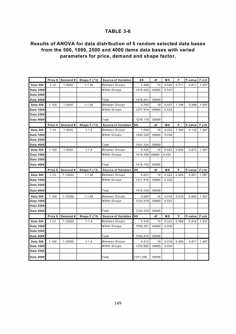
149
TABLE 3-6
Results of ANOVA for data distribution of 5 random selected data bases
from the 500, 1000, 2500 and 4000 items data bases with varied
parameters for price, demand and shape factor.
Price $ Demand # Shape F.(^2) Source of Variation SS df M S F P-value F crit
Data 500 1-10 1-5000 1-1.45 Between Groups 0.499 19 0.026 0.711 0.811 1.587
Data 1000 W ithin Groups 1475.942 39980 0.037
Data 2500
Data 4000 Total 1476.441 39999
Data 500 1-100 1-5000 1-1.45 Between Groups 0.702 19 0.037 1.156 0.286 1.587
Data 1000 W ithin Groups 1277.474 39980 0.032
Data 2500
Data 4000 Total 1278.176 39999
Price $ Demand # Shape F.(^2) Source of Variation SS df M S F P-value F crit
Data 500 1-10 1-5000 1-1.4 Between Groups 1.006 19 0.053 1.365 0.132 1.587
Data 1000 W ithin Groups 1550.329 39980 0.039
Data 2500
Data 4000 Total 1551.334 39999
Data 500 1-100 1-5000 1-1.4 Between Groups 0.436 19 0.023 0.646 0.873 1.587
Data 1000 W ithin Groups 1418.299 39980 0.035
Data 2500
Data 4000 Total 1418.735 39999
Price $ Demand # Shape F.(^2) Source of Variation SS df M S F P-value F crit
Data 500 1-10 1-10000 1-1.45 Between Groups 0.421 19 0.022 0.625 0.891 1.587
Data 1000 W ithin Groups 1417.818 39980 0.035
Data 2500
Data 4000 Total 1418.239 39999
Data 500 1-100 1-10000 1-1.45 Between Groups 0.299 19 0.016 0.510 0.960 1.587
Data 1000 W ithin Groups 1232.079 39980 0.031
Data 2500
Data 4000 Total 1232.378 39999
Price $ Demand # Shape F.(^2) Source of Variation SS df M S F P-value F crit
Data 500 1-10 1-10000 1-1.4 Between Groups 0.435 19 0.023 0.588 0.918 1.587
Data 1000 W ithin Groups 1556.381 39980 0.039
Data 2500
Data 4000 Total 1556.816 39999
Data 500 1-100 1-10000 1-1.4 Between Groups 0.313 19 0.016 0.480 0.971 1.587
Data 1000 W ithin Groups 1370.985 39980 0.034
Data 2500
Data 4000 Total 1371.298 39999

150
3.4 Chapter Summary
Although the previous discussion has established that data base domains
remain similar over time and error terms are within narrow boundaries, it
requires additional data base analysis to confirm the generalisability of the
model’s prediction ability as to error detection.
In the next chapter a number of organisational data bases are analysed for
both domain consistency and data element accuracy.
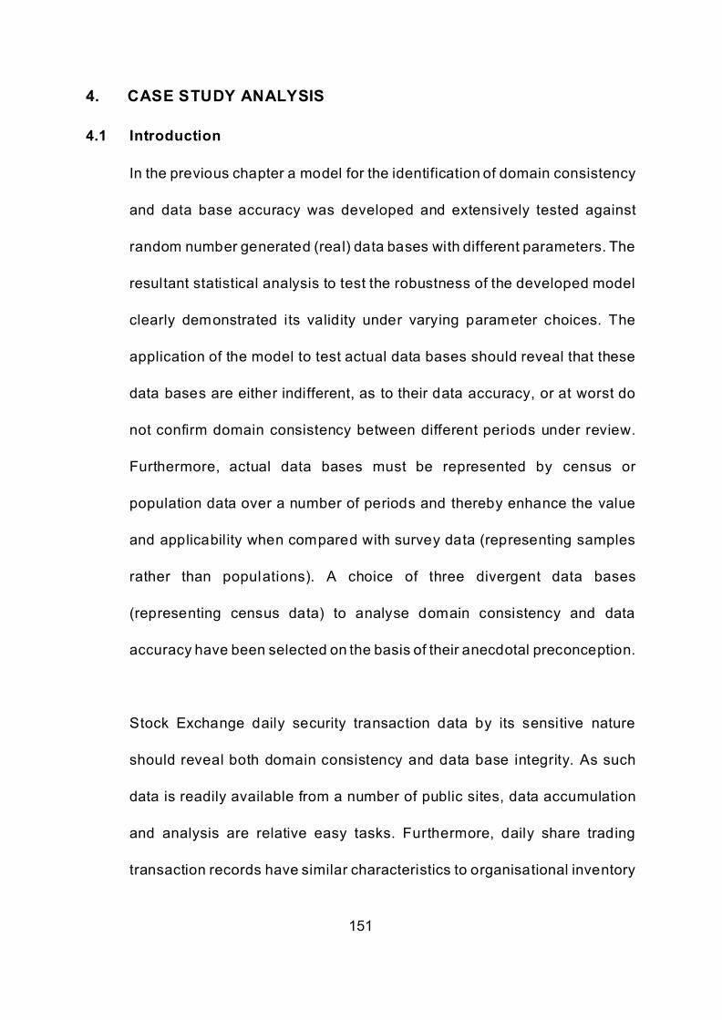
151
4. CASE STUDY ANALYSIS
4.1 Introduction
In the previous chapter a model for the identification of domain consistency
and data base accuracy was developed and extensively tested against
random number generated (real) data bases with different parameters. The
resultant statistical analysis to test the robustness of the developed model
clearly demonstrated its validity under varying parameter choices. The
application of the model to test actual data bases should reveal that these
data bases are either indifferent, as to their data accuracy, or at worst do
not confirm domain consistency between different periods under review.
Furthermore, actual data bases must be represented by census or
population data over a number of periods and thereby enhance the value
and applicability when compared with survey data (representing samples
rather than populations). A choice of three divergent data bases
(representing census data) to analyse domain consistency and data
accuracy have been selected on the basis of their anecdotal preconception.
Stock Exchange daily security transaction data by its sensitive nature
should reveal both domain consistency and data base integrity. As such
data is readily available from a number of public sites, data accumulation
and analysis are relative easy tasks. Furthermore, daily share trading
transaction records have similar characteristics to organisational inventory

152
records as a number of securities are not traded every day whereas others
are traded on a daily basis but with different volumes. These daily changes
can be associated with an organisation’s inventory records where annual
product changes may experience similar patterns.
A second data base that also presents a data base item change on an
annual basis is university student enrolment records. The number of
students enrolled in different programs and subjects from year to year
differs as well as new programs being offered while some of the less
supportable programs may either be abandoned or combined with other
more viable programs. As the majority of Australian universities are public-
funded institutions, a biannual consolidation of student enrolment data by
government funding agencies becomes a prerequisite condition for funds
distribution. Since its restructured funding formula in the early 1990s none
of the 39 publicly funded universities ever reported a reduction in student
enrolment data according to comments offered by financial staff of the
Department of Education, Science and Training (DEST). Such anecdotal
evidence would suggest that student enrolment data is well managed by
university administrators but is likely to contain both domain as well as data
item inaccuracies that should be detectable through the application of the
model developed in the previous chapter.

153
The third of the data bases analysed by the developed model comes from
the inventory records of an Australian subsidiary of a multinational
company. The data was taken from existing company records for the period
from 1993 to 1998. Although the recorded period comprises six years only,
three years were selected for data analysis as the data inaccuracies in the
other three years were identified by company officers but remained
uncorrected. The company intended to restructure and consolidate a
number of product-based data bases to reduce the recognised data
inaccuracy between individual data bases established for different
functional responsibilities. While production-based data was recorded for
the purpose of product manufacture scheduling, inventory records were
based on actual sales with substantial item detail differences between
these data bases. In addition the company employed a rather unusual
overhead allocation system by combining raw materials and some direct
labour hours as basis for overhead allocations to individual products. The
cost-pool for determining overhead costs was also inconsistent with
accumulating some product related direct labour hours as well as more
traditional indirect costs. While total product costs appeared to represent
a realistic cost level, a number of product items varied substantially from
one period to the next without evidence in production process or raw
material changes. This data base is used to not only test the data base

8
http: //www.intersuisse.com.au/shareprices2_frames.htm, data from this source was downloaded on a daily basis.
The data contains only those s hares that were traded during the day and not the com plete listing. T he number of
shares traded during the 14 day period ranged from 723 to 761. Investigation of each of the daily records revealed
a number of securities were listed but had no transaction rec ords . W hen the com pany that produces these records
was contacted it was explained that transactions are listed in m ultiples of 1000 and that the listed securities w ith
0 transaction entries may have been trading in less than marketable parcels.
154
integrity and accuracy but applies the model generated values to assign
overhead costs to individual products.
The Stock Exchange and University data, although selected from different
sectors of the Economy representing service industries, display similar
characteristics to the manufacturing industry inventory data base
characteristics over a number of periods. The model can, therefore, also be
applied to these industries for the allocation of discretionary costs
(overhead costs) to selected activity centres.
4.2 Case Study Analysis Stock Exchange Data.
A readily accessible data base that displays similar characteristics to
inventory movements in organisations is the daily share trading
transactions of major stock exchanges. Share trading data (share
transactions by volume and value from the Sydney Stock Exchange,
Australia8) over a period of seven days (August 31 to September 10) were
evaluated to determine if pattern similarity does exist. While the daily share
trading deals with a large number of transactions in the same securities are
considerable, there are a discernable number of shares that are unique to

155
a day’s trading pattern. In addition, changes in the number of specific
securities together with their price fluctuations mirror product characteristics
of demand and competition induced price adjustments. Table 4-1 shows the
results of the ANOVA-test together with the critical values at the 20% share
number level for each of the (7) days.
Table 4-1,
Results of ANOVA for Australian Share data("=.05)Source of
Variation
SS df M S F P-value F crit
Between Groups 0.093 6 0.015 0.601 0.730 2.100
W ithin Groups 132.419 5159 0.026
Total 132.512 5165
Day 1 2 3 4 5 6 7
at 20% (x) 83.24% 84.72% 83.54% 84.33% 84.90% 85.10% 83.63%
As the F value is well within the critical limit, the seven day data clearly
demonstrates domain consistency (data base integrity) which is expected
from such data base. Domain consistency refers to data from different
periods displaying similar pattern consistency and therefore must be judged
to come from the same organisation.
Table 4-2,
F-test for daily transactions/model values("=.05)
Date
Parameter
Aug
31
Sept
2
Sept
3
Sept
6
Sept
7
Sept
8
Sept
13
F 1.490 1.170 1.122 1.054 1.069 1.080 1.430
P-value 0.000 0.015 0.059 0.238 0.181 0.127 0.000
F-crit. 1.128 1.127 1.128 1.130 1.129 1.130 1.128
N 746 761 747 728 739 723 748

156
However, when the transaction data for each of the seven days is
compared with the model generated values and for three of the seven days
(Aug. 31, Sept 2 and Sept 13) the results indicate statistical significance as
shown in Table 4-2. Such indication suggests data base inaccuracy. On
contacting the organisation that compiles the stock exchange transaction
data it was revealed that inaccuracies are possible as some of the traded
securities are traded in non marketable parcels and that aggregation for
data base inclusion may lead to recorded inaccuracies. It was further
revealed that it is possible to omit some of the traded shares due to delays
in private broker recording of transactions.
4.3 Case Study Analysis University Enrolment Data
Although the previous case study example demonstrates the inherent
hazard in using existing data base data for future predictions of component
characteristics and behaviour, another type of data base that requires
accuracy but maybe open to unchecked acceptance by funding authorities
can be found in the Australian higher education sector. The Australian
higher education sector is dominated by government funded public
universities. W ith such a funding structure it is necessary to submit
semester-based student enrolment data to a central authority for
substantiating the allocated funds from public sources. The Department of
Education, Science and Training [DEST] is the collector of such data on a

9
The data collection by DEST is based on two cut-off dates(31st of March-Autumn semester and 31s t of August-
Spring sem ester) f or each of the semes ters and requ ires universities to subm it their actual student enrolment data
for each of the sub jec ts of fered by the university. As there is a substantial var iety in student records systems
accross the Aus tralian univers ity sec tor it is not uncommon that the reported student enrolments at the cut-off dates
vary from the actual classroom numbers.
10
T his was confirmed by a DEST officer in an telephone interview conducted on the 22-5-2002. The amou nt is
approximately equivalent to the Higher Education Contribution Component [HECS] but in any case A$ 2,600 per
EFTSU .
157
biannual basis9 to maintain accurate records for statistical analysis and
justification for funding. However, individual university funding is based on
a student/program profile that estimates the number of enrolments in
equivalent full time students units (EFTSU) established in 1990 and
provides marginal funding10 for reported over enrolled students. As under
enrolment is penalised with a deduction from operating funding allocations
equivalent to the marginal funding amount it is unusual for universities to
report under enrolments. It is more common for universities to report over
enrolments to at least attract the marginal funding allocation. DEST does
conduct internal audits to reconcile reported data with profile data but has
only limited opportunities to check the reported data accuracy submitted by
universities.
As each university is required to submit their data in subject and student
enrolment groupings it is of interest to check a random sample of university
data bases to ascertain both domain consistency and data base integrity by
applying and statistically comparing the model computed values with those
of the actual data records. DEST supplied the data for 12 universities that
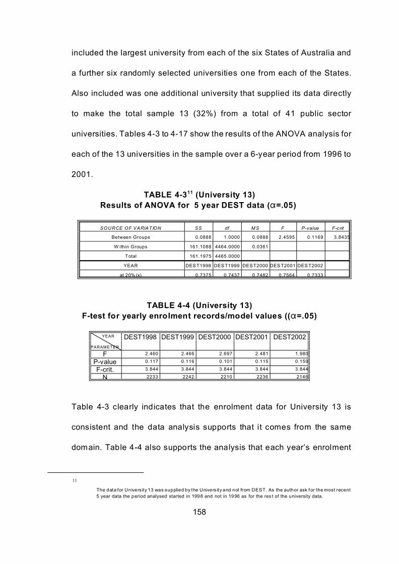
11
The data for University 13 was supplied by the University and not from DEST. As the author ask f or the most recent
5 year data the period analysed started in 1998 and not in 1996 as for the res t of the university data.
158
included the largest university from each of the six States of Australia and
a further six randomly selected universities one from each of the States.
Also included was one additional university that supplied its data directly
to make the total sample 13 (32%) from a total of 41 public sector
universities. Tables 4-3 to 4-17 show the results of the ANOVA analysis for
each of the 13 universities in the sample over a 6-year period from 1996 to
2001.
TABLE 4-311 (University 13)
Results of ANOVA for 5 year DEST data ("=.05)
SOURCE OF VARIATION SS df MS F P-value F-c rit
Between Groups 0.0888 1.0000 0.0888 2.4595 0.1169 3.8435
W ithin Groups 161.1088 4464.0000 0.0361
Total 161.1975 4465.0000
YEAR DES T1998 DES T1999 DES T2000 DES T2001 DES T2002
at 20% (x) 0.7375 0.7437 0.7482 0.7564 0.7333
TABLE 4-4 (University 13)
F-test for yearly enrolment records/model values (("=.05)
YEAR
PARAMETER
DEST1998 DEST1999 DEST2000 DEST2001 DEST2002
F 2.460 2.466 2.697 2.481 1.980
P-value 0.117 0.116 0.101 0.115 0.159
F-crit. 3.844 3.844 3.844 3.844 3.844
N 2233 2242 2210 2236 2146
Table 4-3 clearly indicates that the enrolment data for University 13 is
consistent and the data analysis supports that it comes from the same
domain. Table 4-4 also supports the analysis that each year’s enrolment

159
data when compared with model generated values shows no statistical
significant differences as each of the p-values is clearly above the level of
significance ("=.05). The values for each of the 12 Universities that was
supplied by the (DEST) database are shown in tables 4-5 to 4-17.

160
Table 4-5ANOVA FOR EACH OF THE 12 UNIVERSITIES’ 5 YEAR STUDENTS ENROLMENT RECORDS
University Source of Variation SS df MS F P-value F crit
Between Groups 0.1549 5 0.0309 0.7502 0.5858 2.2147
Within Groups 550.1011 13319 0.0413
1 Total 550.2560 13324
Year DEST1996 DEST1997 DEST1998 DEST1999 DEST2000 DEST2001
at 20%(x) 70 71.55% 71 70 72.42% 73
Between Groups 0.2524 5 0.0504 1.1042 0.3556 2.2149
Within Groups 503.9953 11023 0.0457
2 Total 504.2477 11028
Year DEST1996 DEST1997 DEST1998 DEST1999 DEST2000 DEST2001
at 20%(x) 66 67.71% 69.03% 70.11% 69.18% 69.45%
Between Groups 1.5615 5 0.3123 8.0096 0 2.2145
Within Groups 859.0447 22031 0.0389
3 Total 860.6063 22036
Year DEST1996 DEST1997 DEST1998 DEST1999 DEST2000 DEST2001
at 20%(x) 66 68.01% 69.05% 68.78% 71.12% 72.22%
Between Groups 1.5315 5 0.3063 5.2622 0 2.2174
Within Groups 157.5125 2706 0.0582
4 Total 159.0440 2711
Year DEST1996 DEST1997 DEST1998 DEST1999 DEST2000 DEST2001
at 20%(x) 52.41% 48.94% 54.34% 58.01% 62.31% 60
Between Groups 0.9111 5 0.1822 4.5303 0.0004 2.2148
Within Groups 503.8771 12527 0.0402
5 Total 504.7882 12532
Year DEST1996 DEST1997 DEST1998 DEST1999 DEST2000 DEST2001
at 20%(x) 64.87% 67.14% 68.76% 69.44% 70.55% 69.11%
Between Groups 0.2785 5 0.0557 1.3173 0.2533 2.2147
Within Groups 590.8926 13974 0.0422
6 Total 591.1711 13979
Year DEST1996 DEST1997 DEST1998 DEST1999 DEST2000 DEST2001
at 20%(x) 68 67.47% 69.32% 70.51% 70.83% 69.11%
Between Groups 0.1947 5 0.0389 0.8668 0.5023 2.2147
Within Groups 575.1384 12802 0.0449
7 Total 575.3331 12807
Year DEST1996 DEST1997 DEST1998 DEST1999 DEST2000 DEST2001
at 20%(x) 68.35% 68.60% 68.88% 70.17% 69.65% 70.80%
Between Groups 1.0274 5 0.2054 5.3321 0 2.2144
Within Groups 929.8271 24127 0.0385
8 Total 930.8546 24132
Year DEST1996 DEST1997 DEST1998 DEST1999 DEST2000 DEST2001
at 20%(x) 71.15% 71.31% 72.19% 73.39% 74.03% 75.35%
Between Groups 2.8003 5 0.56 14.5976 0 2.2145
Within Groups 712.5457 18572 0.0383
9 Total 715.346 18577
Year DEST1996 DEST1997 DEST1998 DEST1999 DEST2000 DEST2001
at 20%(x) 67.32% 70.17% 72.04% 73.76% 74.92% 74.50%
Between Groups 1.4498 5 0.2899 6.3894 0 2.2145
Within Groups 967.3126 21314 0.0453
10 Total 968.7625 21319
Year DEST1996 DEST1997 DEST1998 DEST1999 DEST2000 DEST2001
at 20%(x) 73.48% 69.66% 68.24% 69.30% 70.27% 69.00%
Between Groups 0.2805 5 0.0561 1.375 0.2301 2.2143
Within Groups 1211.8667 29697 0.0408
11 Total 1212.1473 29702
Year DEST1996 DEST1997 DEST1998 DEST1999 DEST2000 DEST2001
at 20%(x) 70.37% 70.81% 70.34% 69.21% 68.35% 69.18%
Between Groups 0.2131 5 0.0426 1.0784 0.3699 2.2143
Within Groups 1436.3967 36345 0.0395
12 Total 1436.6098 36345
Year DEST1996 DEST1997 DEST1998 DEST1999 DEST2000 DEST2001
at 20%(x) 74.12% 73.61% 73.04% 73.05% 73.96% 74.73%
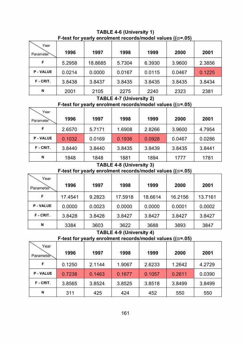
161
TABLE 4-6 (University 1)
F-test for yearly enrolment records/model values (("=.05)
Year
Parameter 1996 1997 1998 1999 2000 2001
F 5.2958 18.8685 5.7304 6.3930 3.9600 2.3856
P - VALUE 0.0214 0.0000 0.0167 0.0115 0.0467 0.1225
F - CRIT. 3.8438 3.8437 3.8435 3.8435 3.8435 3.8434
N 2001 2105 2275 2240 2323 2381
TABLE 4-7 (University 2)
F-test for yearly enrolment records/model values (("=.05)
Year
Parameter 1996 1997 1998 1999 2000 2001
F 2.6570 5.7171 1.6908 2.8266 3.9600 4.7954
P - VALUE 0.1032 0.0169 0.1936 0.0928 0.0467 0.0286
F - CRIT. 3.8440 3.8440 3.8435 3.8439 3.8435 3.8441
N 1848 1848 1881 1894 1777 1781
TABLE 4-8 (University 3)
F-test for yearly enrolment records/model values (("=.05)
Year
Parameter1996 1997 1998 1999 2000 2001
F 17.4541 9.2823 17.5918 18.6614 16.2156 13.7161
P - VALUE 0.0000 0.0023 0.0000 0.0000 0.0001 0.0002
F - CRIT. 3.8428 3.8428 3.8427 3.8427 3.8427 3.8427
N 3384 3603 3622 3688 3893 3847
TABLE 4-9 (University 4)
F-test for yearly enrolment records/model values (("=.05)
Year
Parameter1996 1997 1998 1999 2000 2001
F 0.1250 2.1144 1.9067 2.6233 1.2642 4.2729
P - VALUE 0.7238 0.1463 0.1677 0.1057 0.2611 0.0390
F - CRIT. 3.8565 3.8524 3.8525 3.8518 3.8499 3.8499
N 311 425 424 452 550 550
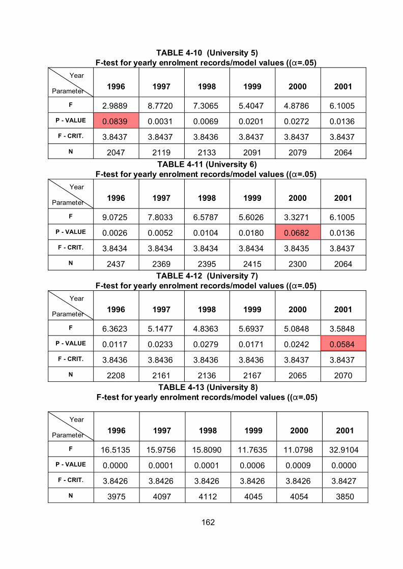
162
TABLE 4-10 (University 5)
F-test for yearly enrolment records/model values (("=.05)
Year
Parameter1996 1997 1998 1999 2000 2001
F 2.9889 8.7720 7.3065 5.4047 4.8786 6.1005
P - VALUE 0.0839 0.0031 0.0069 0.0201 0.0272 0.0136
F - CRIT. 3.8437 3.8437 3.8436 3.8437 3.8437 3.8437
N 2047 2119 2133 2091 2079 2064
TABLE 4-11 (University 6)
F-test for yearly enrolment records/model values (("=.05)
Year
Parameter1996 1997 1998 1999 2000 2001
F 9.0725 7.8033 6.5787 5.6026 3.3271 6.1005
P - VALUE 0.0026 0.0052 0.0104 0.0180 0.0682 0.0136
F - CRIT. 3.8434 3.8434 3.8434 3.8434 3.8435 3.8437
N 2437 2369 2395 2415 2300 2064
TABLE 4-12 (University 7)
F-test for yearly enrolment records/model values (("=.05)
Year
Parameter1996 1997 1998 1999 2000 2001
F 6.3623 5.1477 4.8363 5.6937 5.0848 3.5848
P - VALUE 0.0117 0.0233 0.0279 0.0171 0.0242 0.0584
F - CRIT. 3.8436 3.8436 3.8436 3.8436 3.8437 3.8437
N 2208 2161 2136 2167 2065 2070
TABLE 4-13 (University 8)
F-test for yearly enrolment records/model values (("=.05)
Year
Parameter1996 1997 1998 1999 2000 2001
F 16.5135 15.9756 15.8090 11.7635 11.0798 32.9104
P - VALUE 0.0000 0.0001 0.0001 0.0006 0.0009 0.0000
F - CRIT. 3.8426 3.8426 3.8426 3.8426 3.8426 3.8427
N 3975 4097 4112 4045 4054 3850

163
TABLE 4-14 (University 9)
F-test for yearly enrolment records/model values (("=.05)
Year
Parameter1996 1997 1998 1999 2000 2001
F 19.4158 13.4952 8.9257 7.1486 6.1205 7.5652
P - VALUE 0.0000 0.0002 0.0028 0.0075 0.0134 0.0060
F - CRIT. 3.8427 3.8428 3.8430 3.8431 3.8431 3.8431
N 3605 3359 3087 2882 2886 2759
TABLE 4-15 (University 10)
F-test for yearly enrolment records/model values (("=.05)
Year
Parameter1996 1997 1998 1999 2000 2001
F 5.8657 8.0663 7.7396 6.2316 6.9143 10.1128
P - VALUE 0.0155 0.0045 0.0054 0.0126 0.0086 0.0015
F - CRIT. 3.8428 3.8429 3.8429 3.8428 3.8427 3.8426
N 3533 3190 3207 3504 3819 4064
TABLE 4-16 (University 11)
F-test for yearly enrolment records/model values (("=.05)
Year
Parameter1996 1997 1998 1999 2000 2001
F 7.8837 14.2321 14.8194 18.4598 18.0419 16.7161
P - VALUE 0.0050 0.0002 0.0001 0.0000 0.0000 0.0000
F - CRIT. 3.8423 3.8423 3.8424 3.8424 3.8425 3.8425
N 5454 5389 5112 4790 4503 4455
TABLE 4-17 (University 12)
F-test for yearly enrolment records/model values (("=.05)
Year
Parameter1996 1997 1998 1999 2000 2001
F 8.4186 9.4605 13.4837 12.2944 9.1065 7.8838
P - VALUE 0.0037 0.0021 0.0002 0.0005 0.0026 0.0050
F - CRIT. 3.8423 3.8423 3.8422 3.8422 3.8422 3.8422
N 5595 5810 6368 6211 6200 6167

164
Of the 13 universities investigated for student data record integrity only one
passed the ANOVA test for both domain integrity and annual student
enrolment data accuracy. Of the remaining 12 universities one other could
be identified for domain integrity and student enrolment data accuracy for
three of the 6-year recording period. University 4s results are unusual in
that it does not indicate domain integrity but shows student enrolment data
accuracy for five of the 6-year recording period. All other universities show
statistically significant differences in student enrolment data records while
only seven of the 13 universities indicate domain integrity. W hile the
statistical analysis cannot determine the direction of the student enrolment
data inaccuracy, by implication it would appear that most of the
inaccuracies are skewed toward the over reporting rather than under
reporting. This assumption can be supported by the comment provided by
a DEST financial officer in stating that she was unaware of any under
reporting by universities since the establishment of the original university’s
profile. The suggestion here is that most university administrations are
more likely to over report as such strategy provides additional marginal
funding rather than a reduction in funding through under reporting student
enrolments.
An example may clarify the strategy pursued by universities. University (A)
has an enrolment profile established by DEST in 1991 of 12,000 for its then

165
existing program structure. Additional approved programs will attract
additional government funding as the expected student enrolments are
expected to increase to a figure of 12,000 plus X. As university
administrators are familiar with the DEST profile for their university,
changes in student enrolment trends are projected as increasing at a
positive rate. Competition for students amongst universities, especially in
geographical areas were more then one university is accessible by
prospective students, may lead to negative trending of student enrolments
and therefore to reduced funding. Given the competition for public
education funding university administrators are reluctant to report negative
trending enrolment data.
It is, therefore, suggested that university administrators who are familiar
with the established profile for their university would try to match their
enrolment data with profile expectations rather than the accurate enrolment
data at the predetermined cut-off dates. Although, university administrators
are responsible for the reporting of enrolment data, such data is often
provided by academics in charge of subjects. In some cases there may
also be an incentive by academics responsible for subject administration
to report student numbers in excess of actual enrolments to maintain
marginal subject funding and to maintain subject viability.
166
DEST has only limited resources to detect reported enrolment data
inaccuracies and relies on profile projected comparisons for questioning
data supplied by universities. Given the number of competing interests that
are involved in the recording of student enrolment data it is difficult for
funding authorities to provide the necessary incentives to universities to
establish internal record keeping systems that portray a more accurate
reflection of the actual student enrolments.
In summary, it has been demonstrated that the accuracy of recorded data
is questionable. Reasons for inaccurate data recording are multi faceted
and range from entry and omission errors (stock exchange data) to data
manipulations to reflect desired outcomes (university student enrolment
data).
4.3 Case Study Analysis Inventory Data
While there is limited empirical evidence as to unbalanced distribution
patterns within organisational inventory data bases from one period to
another, using the (3) year inventory record of the case data tends to
support the proposition that a firm’s inventory data base distribution shows
no significant variation. Evaluation of product data on the basis of cost
reduces the bias of revenue analysis caused by varying profit margins.
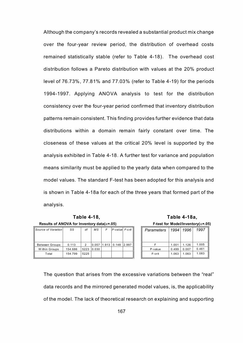
167
Although the company’s records revealed a substantial product mix change
over the four-year review period, the distribution of overhead costs
remained statistically stable (refer to Table 4-18). The overhead cost
distribution follows a Pareto distribution with values at the 20% product
level of 76.73%, 77.81% and 77.03% (refer to Table 4-19) for the periods
1994-1997. Applying ANOVA analysis to test for the distribution
consistency over the four-year period confirmed that inventory distribution
patterns remain consistent. This finding provides further evidence that data
distributions within a domain remain fairly constant over time. The
closeness of these values at the critical 20% level is supported by the
analysis exhibited in Table 4-18. A further test for variance and population
means similarity must be applied to the yearly data when compared to the
model values. The standard F-test has been adopted for this analysis and
is shown in Table 4-18a for each of the three years that formed part of the
analysis.
Table 4-18, Table 4-18a,
Results of ANOVA for Inventory data("=.05) F-test for Model/Inventory("=.05)
Source of Variation SS df MS F P-value F-c rit
Parameters 1994 1996 1997
Between Groups 0.113 2 0.057 1.913 0.148 2.997 F 1.001 1.126 1.005
W ithin Groups 154.686 5223 0.030 P-value 0.499 0.007 0.461
Total 154.799 5225 F-cr it 1.063 1.063 1.083
The question that arises from the excessive variations between the “real”
data records and the mirrored generated model values, is, the applicability
of the model. The lack of theoretical research on explaining and supporting

168
the Pareto rule as a law based on scientific replication consistency reduces
the generalisability of the presented case study data base analysis. The
application of the model was based on a subjective choice of a focal point
(the choice of the 20% (x) dimension) to mirror the existing unbalanced data
item distribution. While the initial data pair (0%/0%) and the terminal pair
(100%/100%)is not in dispute and fixed, it is the choice of focal data pair
that can invoke critical commentary as to the validity of the model’s
application.
To reduce this perceived subjectivity of focal point choice, a selection of
different focal points ranging from 10% to 70% (of x values) in 10%
intervals may produce the desired consistency of model applicability.
From the table it is noted that the results for 1994 and 1997 are not
significant indicating that the inventory distribution pattern is not statistically
different from the model values. The 1996 results, however, reveal a
significant deviation and on investigation it was found that the inventory
records for that year were incomplete and not adjusted for mistakes in data
recording. Adjustments to the data base would be accomplished at some
future period by company officers. Although statistically the results revealed
a notable inconsistency between the company’s data base and the model
generated values it did, however, confirm that the inconsistency was

169
attributable to indifferent data capture rather than a loss of model
robustness.
Table 4-19
Model parameters for Case study data
Total O/H Cos ts $2,215,376.00 $2,289,604 $1,885,286
Year 1994 1996 1997
n 1742 1792 1932
Criteria DLH MAT. O/Head DLH* MAT. O/Head DLH MAT. O/Head
20%(x) 76.69% 86.75% 76.73% 86.45% 77.81% 76.70% 88.54% 77.03%
Rank (1) 2.22% 4.32% 2.22% 4.49% 4.02% 1.92% 5.09% 1.88%
c 7.116 9.149 7.111 9.3162 9.3787 6.9678 9.9268 6.9474
d .2668 .2443 .2678 .2299 .1618 .281 .2226 0.2883
17.0471 5.281 17.223 4.2158 1.5267 22.72 3.114 24.2259
Model Com parison (ANOVA analysis)
F-tes t ("=.05) 2.246 .8698 1.4405 .2829 3.5035 5.677 .135 4.677
F-c ritical 3.844 3.844 3.844 3.844 3.844 3.844 3.844 3.844
P value .134 .351 .2301 .5948 .0613 .0172 .713 0.0306
* data for d irect labour was incom plete and rec ords were not available to reconstruct the production data.
In Table 4-19 the computed model parameters for the three years under
review are shown. The values were computed with the aid of a standard
spreadsheet optimisation function and are based on the ranking of actual
direct labour hours, direct materials and overhead allocations. Although it
was demonstrated earlier (refer to Table 2-6) that the relationship between
direct labour hours and overhead costs under both traditional and ABC
based overhead distributions have a high correlation (r= .92 and .94
respectively) and therefore can be considered as a good proxy for model
parameter computation and comparison, the current case study data
revealed substantial inconsistencies in data recording and rendered direct
labour hours an unreliable proxy for purposes of comparison.

170
Table 4-20 presents the results of the data comparison for three randomly
selected items from the inventory records for each of the three years under
review. The ranking column in Table 4-20 is based on the rank of the
selected items within the direct material sorted data base. Three randomly
selected items one from each of the high, medium and low volume
production was selected for comparison and substantial variations between
the actual overhead and the computed overhead values were identified.
When these variations were discussed with the production manager of the
company, it became evident that the internal records had not been
maintained properly and overhead allocations were based on material and
labour combinations that explained the inconsistency of the data. Further
interviews with the management accountant revealed that the company
maintained separate data bases for production control and inventory
records and a consolidation and between these data bases was not part of
the internal control system structure. The company is introducing a new
software package and hopes that the detected inconsistencies in overhead
allocations will be resolved through the application of the package which
provides the opportunity of data base consolidation and record comparison.
However, what has been demonstrated by the inventory record analysis is
the model’s ability to rank a related variable (direct material) and apply the
item percentage contribution to the computation of overhead allocations

171
rather than relying on direct labour hours as a ranking base for such
computed allocations. The use of direct material as a ranking variable
provides the additional benefit of a clearer audit trail to establish objectivity
of data rather than the direct labour hour data if it is reliant on recorded
rather than standard costing compilations. What is, however, of interest is
the substantial variation in recorded as compared to computed costs and
would suggest that the inherent inconsistencies in overhead allocations
should not be attributed to the technique of applying single volume based
cost drivers (absorption costing) but rather the indifference of the prevailing
data recording system.
In chapter 3 it was established that the expected confidence limit between
“real” and model computed values at the 95% confidence level has an
upper and lower limit of -2.2% and +1.3% it is, therefore, possible to apply
this confidence interval to the data in Table 4-20 to determine the
magnitude of error that is present in the inventory data base.
TABLE 4-20
Cost Allocation Variances (Actual v Confidence Limits)
Product Year Demand Rank Ac tual Costs Model Cos ts Con f. Interval Variance
Material Total Un it Total Unit low high under over
1994 8149 12 $37,001 $4.54 $27,913 $3.42 $ 3.35 $ 3.46 31.20%
13801 1996 11333 6 $57,472 $5.07 $49,684 $4.38 $ 4.28 $ 4.44 14.20%
1997 1538 94 $6,492 $4.22 $3,959 $2.57 $ 2.51 $ 2.60 62.30%
1994 2 1732 $50 $25.00 $47 $23.26 $ 22.74 $ 23.56 6.11%
T7774H10PN 1996 4 1017 $1,149 $287.25 $151 $37.78 $ 36.94 $ 38.27 650.00%
1997 6 800 $1,791 $298.50 $173 $28.90 $ 28.26 $ 29.28 919.00%
1994 340 359 $715 $1.41 $800 $2.35 $ 2.30 $ 2.38 61.30%
T19MS4 1996 173 527 $293 $1.69 $428 $2.47 $ 2.42 $ 2.50 69.83%
1997 100 791 $141 $1.41 $185 $1.85 $ 1.81 $ 1.87 77.90%

172
The results in Table 4-20 are indicative of a lack of data base integrity
given the extreme large variations between the actual values and those that
were computed by the model applied to the original data for each of the
periods. Another interesting observation concerns the commonly advanced
argument that traditional cost accounting methods tend to overcost high
volume products when compared to ABC overhead cost assignments.
Table 4-20 shows that, although the high volume product (13801) is over
costed, the low volume product (T7774H10PN) is also overcosted by a
substantial margin, whereas the medium volume product (T19MS4) is
under costed.
Organisational inventory records are unlikely to be manipulated to achieve
some desirable outcome and it, therefore, can be assumed that data base
inaccuracy is a result of indifferent data recording or general omissions.
Research evidence relating to data entry errors in general terms suggest
an error range of between 4% and 8% (Valenstein and Meier, 1999;
Swanson et.al., 1997; Stanton and Julian, 2002; Jørgensen and Karlsmose,
1998). The substantial number of errors detected in the database of the
organisation in both their inventory and production records was confirmed
by the management accountant and is usually adjusted at the end of a
period if detected. Error detection of recorded data, however, is not a
priority in the company’s operation.

173
4.4 Chapter Summary
The analysis of three specific data bases (case studies) were selected for
their perceived data integrity and to test the robustness of the model
against actual, rather than random number generated, data bases.
Statistical analysis establishes the accuracy of data element attributes as
well as identifying domain consistencies. While the outcome of the analysis
was predicted, the results were still somewhat surprising.
The Stock Exchange data revealed data element inaccuracies, it confirmed,
however, domain consistencies. The data element inaccuracies are
surprising as daily transaction data is audited prior to the completion of the
trading day.
The university student enrolment records are the most difficult to explain.
W ith the exception of a single university most of the other universities
showed either data base inaccuracies or at worst both domain and data
record inaccuracies. Such findings should be of some concern especially
as a number of universities indicate domain inconsistencies which are
indicative that the recorded data does not come from the same university.
These findings maybe of interest to DEST as the public funding authority
for universities and their resource consumption.

174
The inventory data base also revealed data element inaccuracies but
showed domain consistency. Such finding was expected although inventory
records of public companies are audited prior to financial statement
publication.
Applying the computed model values to the inventory data base provided
the basis for overhead allocations that became situation specific. Earlier
analysis exposed that direct labour records were inaccurate and therefore
an inappropriate base for overhead allocations. As the majority of the
company’s product range consists of a 55% to 75% material cost
component the use of a material ranked distribution became an appropriate
cost driver for the overhead cost allocation.
Taking a random selected sample of high, medium and low demand
products further confirmed the claimed proposition of a more equitable
allocation method. Comparing the computed overhead allocations with the
existing overhead cost revealed under and over costed allocations. While
ABC comparisons with traditional cost allocation models consistently
demonstrate an over costed overhead allocation for high volume/low
complexity products and an under costed overhead allocation for low
volume/high complexity products (Pattinson and Arendt, 1994), the model
based allocation does not confirm such consistent variation. The inventory

175
case study data shows that both high and low demand products are over
costed while medium demand products appear to be under costed when
compared with actual overhead cost data.

176
5. Discussion of Results
In chapter 4 it was established that data base inconsistencies could be
addressed by the development of a model that allows the mirroring of a real
data base and use the model as a benchmark test for data base i tem
variation within acceptable boundaries. The parameters of the model were
based on the empirical evidence that almost all recorded data bases follow
an unbalanced item distribution that was first discussed by Pareto, W
(1883) and later picked up by Joseph Juran in the early 1950's as an
analytical approach in the development of quality improvement process.
While the general acceptance of a Pareto based accumulative data item
distribution remains valid, what had not been established is a model that
provides the basis for calculating the individual item contribution as a
method to predict pattern consistencies.
The model developed in Chapter 3 was tested and modified to insure its
robustness under varying data base parameters. Although, there is some
anecdotal (Roadcap et al., 2000) and some empirical evidence (Valenstein
and Meier, 1999; Swanson et al., 1997; Stanton and Julian, 2002;
Jørgensen and Karlsmose, 1998) that suggests data base integrity and
accuracy is diminished through data entry and data omission errors, there
is, however, little research that investigates the accuracy of an established
recorded data base. Given the acceptance that data entry and omission

177
errors exist at a suggested level of between 4% and 8% (Valenstein and
Meier, 1999) it is surprising that there is very little effort to develop models
that allow analysis of existing data bases to detect the level of error that
exists.
To reduce the incidence of data entry and data omission errors in
developing the model, a random number generator approach was used to
establish the original data bases. The developed model was tested against
these data bases through pair wise comparison to establish its robustness
when applied to 3200 different data bases with varying parameters that
included changes in product pricing, product demand and distribution shape
factor. In addition the number of items were varied between 500 and 4000
to reflect medium size inventory levels.
To overcome the limitation of subjectively choosing the 20% focal point of
the (x) dimension a stratified selection of the random generated data bases
were used and additional focal points at the 10%, 30%, 40%, 50%, 60%
and 70% level were submitted to analysis to determine variations in error
levels. The range of error terms at any of these levels remained within the
original range at the 20% level. This analysis clearly established the validity
and robustness of the model and justified the subjective choice of the 20%
level as it is representative of the 20/80 rule discussed in other literature
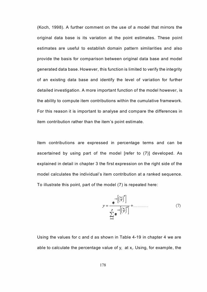
178
(Koch, 1998). A further comment on the use of a model that mirrors the
original data base is its variation at the point estimates. These point
estimates are useful to establish domain pattern similarities and also
provide the basis for comparison between original data base and model
generated data base. However, this function is limited to verify the integrity
of an existing data base and identify the level of variation for further
detailed investigation. A more important function of the model however, is
the ability to compute item contributions within the cumulative framework.
For this reason it is important to analyse and compare the differences in
item contribution rather than the item’s point estimate.
Item contributions are expressed in percentage terms and can be
ascertained by using part of the model [refer to (7)] developed. As
explained in detail in chapter 3 the first expression on the right side of the
model calculates the individual’s item contribution at a ranked sequence.
To illustrate this point, part of the model (7) is repeated here:
Using the values for c and d as shown in Table 4-19 in chapter 4 we are
able to calculate the percentage value of y i at xi. Using, for example, the

179
1994 overhead data with a denominator value of 17.0471, a value for c of
7.116 and a value for d of .2668 we can calculate a percentage value of y i
given the rank of x i. in the example let x = 100, therefore:
This result enables the comparison between the accurate data base values
for each ranked data item and those values generated by the model in a
pair wise analysis. Point estimates compare the cumulative percentage
between actual and model data base values, which given the argument
provided earlier as to the likelihood and risk of data base inaccuracy due
to error entry and data omission would render such comparison as
meaningless and therefore the associated error term would not be
indicative of the robustness of the model.
The creation and testing of a substantial number of random number
generated data bases (3200 in total) revealed a consistency in both
domain identification and error term values that provides significant
evidence that the developed model is capable to detect inconsistencies in
“real” data bases and allows for the identification of element suspicion and
investigation. The model further, and more important, has shown sufficient
180
robustness under varying data base sizes to be applied as a prediction
model for overhead determination of an organisation’s product portfolio.
The advantages from the developed model when compared to many of the
existing techniques used in the determination of overhead prediction is the
continuation of the preferred simplicity (Whittle, 2000) of the absorption
cost model with the added advantage of accounting for product additions
or deletions in a more equitable and product supportive approach.
While product additions are often allowed to add additional variable costs
to the existing costs of an organisation but, if added within the current
capacity level, will not incur any additional fixed overhead costs which will
be treated quite differently under various cost allocation techniques.
Under the absorption cost allocation approach direct labour or some other
single volume allocation base will be employed to compute an arbitrary
value of overhead costs applied to the new product. Variable costing
methods would only add the variable portion of the overhead to the new
product in an attempt to acknowledge that the fixed overhead total costs
remain unchanged within current capacity levels. Activity based costing
methods would identify the activities necessary in the production of the
new product and would use past activity cost data to attach overhead costs
to the product.

181
Product deletions on the other hand are treated similar but with a cost
increasing effect on the remaining products within the organisation’s
product portfolio. This effect was demonstrated in Chapter 4 using the case
study data and the changing overhead costs of three products that were
part of the organisation’s product portfolio over the 4-year history
presented. Investigation of the inventory records revealed a product
retention rate over this period of approximately 70 percent using product
identification codes to determine product portfolio composition. The
inconsistency of applying overhead costs to products is clearly evident for
product 2 in Table 4-20 (T774H10PN) where overhead costs in 1994 were
$25.00 per unit but increased to 287.25 in 1996 and 298.50 in 1997. This
inconsistency, when pointed out to the management accountant of the
organisation at the time, was admitted as being erroneous. Other item
inconsistencies appeared across all the years that data was supplied.
Model calculated values for this item were more consistent and given the
general increases in material prices and labour costs over the period
reflects a more normal change in overhead costs on the basis of material
content.
This approach is a departure from general practice of overhead allocations
based on material content but was found to be the most acceptable
allocation base as material content on average exceeded 70 percent of the

182
products’ costs. This departure also demonstrates the flexibility and
simplicity of the model to become situation specific rather then being a
general fit for all organisations. This general fit of overhead allocation
models (the most popular approach being the absorption cost model) on
the basis of single volume resource bases must be perceived as its major
shortcoming.
While Activity-based cost systems address this shortcoming of general
applicability and complement situation specific circumstances its system
design, however, is founded in the analysis of existing data bases and
subjective based cost driver determination. Furthermore, in chapter 2 it
was pointed out that the ABC suffers from similar problems to any of the
more traditional allocation techniques as the product and facility levels of
the ABC hierarchy also rely on judgement based overhead allocations in
addition to the discussed error creation from designing more disaggregated
cost data systems.
In addition, and as illustrated in chapter 2, different cost allocation methods
become greatly irrelevant, if the organisation pursues a profit optimisation
strategy by fully utilising its available resources. It can therefore be
conjectured that product cost profile determination is useful for single
product (line) decisions on the basis of resource opportunity costs if such

183
decisions lead to increased profitability without a necessary increase in
available capacity. The problem of determining the appropriate overhead
costs for a single product within the totality of an organisation’s product
portfolio has been the subject of much discussion over the years with
different assignment models being available since the problematic nature
of the issue first surfaced. As survey evidence (Whittle, 2000) suggests
most organisations continue to use a simple allocation model to attach
general overhead cost to individual products but uses varying methods
when product related decisions are needed. Such continued persistence
with simplistic allocation models can also be construed as managements
perception that the complexity of an overhead cost assignment model does
not necessarily lead to either greater operational efficiencies or improved
profitability.
The arguments advanced in earlier chapters as to the irrelevance of using
different overhead cost distribution systems can also be leveled against the
proposed Pareto based overhead distribution model. W hat makes the
proposed system any better than ABC or traditional allocation models? The
response to this question is twofold. In the first place it has the ability to
test an existing data base for the integrity of its recorded data and in the
second place provides management with a complementary model similar
to the traditional absorption cost model that has retained its popularity

184
amongst management decision makers, despite the plethora of suggested
“better” overhead assignment models.

185
6. Summary and Future Research Suggestions
6.1 Summary
Research into data base integrity and accuracy has identified the existence
of data base errors being the consequence of numerous causes. Data entry
and data omission errors seem to be the most common causes for data
base inaccuracies. While the majority of the research evidence comes from
medical related publications in which inaccurate data can lead to disastrous
consequences, other data bases such as inventory records receive less
attention as these data bases do not fall within the same categories.
Furthermore, many of the financial data bases are to some extent protected
through the general accepted accounting principle (GAAP) of materiality
that allows organisations to accept inaccurate data base records if such
deviations fall within the acceptable materiality limits which in many cases
are set at the 10% level.
One of the most persistent problems in financial data bases and more
specifically in inventory records has been the application of the
contaminated data detail in the determination of product costs. Although
transaction records are available to verify the accuracy of material and
direct labour costs, overhead costs on the other hand have presented a
problem. As there is no direct connection between a product’s manufacture
(or a service provision) and an organisation’s related indirect costs of

186
resource consumption incurred in the manufacture of a single product,
allocations of these overhead costs were deemed necessary to compute
the total cost of a product. Various techniques for the allocation of an
appropriate amount of such indirect or overhead costs to each single
product or service have been developed and accepted over many years.
The inherent arbitrariness of these techniques has led to continuous and
ongoing criticism and encouraged the development of new techniques that
promise to reduce the arbitrariness factor in the overhead allocation
debate.
Activity-based costing, and to a lesser extent other methods grounded in
operations management, has gained considerable prominence in
contemporary organisational management accounting system designs but
have so far achieved only a limited implementation success. The reason for
such limited implementation by many organisations that are aware of the
claimed advantages of ABC proponents is difficult to explain. While recent
survey evidence indicates the continued popularity and application of the
more traditional and arbitrary overhead allocation methods it does not
explain the reason for rejecting many of the more contemporary overhead
cost system designs.

187
Most of the evidence in support of the necessity to accept and implement
less arbitrary based overhead assignment systems (especially ABC) comes
in the form of case study and similar anecdotal evidence. A common basis
for much of these presentations is the reliance on the organisation’s
existing data records by extending data depositories. ABC is very specific
by insisting that a company’s current record system forms the foundation
of creating activity cost pools that serve as the basis for determining activity
costs by developing and defining appropriate cost drivers for the
computation of activity based costs. There is little evidence that the
establishment of the activity cost pools is free from any of the described
data entry and omission errors and thereby reduces the value of the
developed activity costs.
Other considerations and strategies pursued by organisations do not seem
to be suggestive of the importance of more “accurate” cost data in the
achievement of organisational objectives. A recent, partially longitudinal,
survey (Rigby, 2001) of management tools used does not indicate a
requirement or reliance on financial and management accounting based
data as a desirable tool in the decision making process of organisational
managements. This fact would support the proposition advanced in chapter
3 in which it was demonstrated that optimal profitability is not a function or
consequence of the cost accounting system employed by a company but

188
a function of capacity utilisation and product mix decisions. However,
product mix decision can be based on product cost data as well as capacity
resource consumption. Such considerations would require in most cases
a cost/benefit analysis to determine an optimal outcome.
If it is accepted that product cost data may not assume a dominant position
in management’s decision making process, it is, however, necessary to be
aware of product cost data for product mix related decisions. To
accommodate this desire of management, more reliable product cost data
becomes a prerequisite. When the discussion of distortions in product cost
data is approached, the arbitrariness of the overhead costs allocation
technique is presented as the major contributor to inaccurate product costs.
There is little, if any, discussion about the accuracy of the data collection
methods and the likelihood of corrupted data bases.
The concept of unbalanced or Pareto distributions has been used in many
situations for the analysis of pre-specified relationships of variables of
interest. Pareto analysis of data bases, however, has largely been defined
to a sorting of data elements to establish a dimensional ranking. While this
approach has provided a useful tool in determining value based
relationships it has, however, being restricted to a ranking tool. The ability
to mirror the element ranking contributions through a modeling approach

189
and analyse the paired differences for statistical significance provides a
basis for evaluating the integrity of the original data base. As it has been
suggested in the literature (Valenstein and Meier, 1999; Swanson et.al.,
1997; Stanton and Julian, 2002; Jørgensen and Karlsmose, 1998) most
data bases are likely to contain data recording and data omission errors,
which, given the reliance on such data bases may lead to inappropriate
evaluation of the information these bases contain. To overcome this
inherent risk of using existing data bases for developing a model that can
be tested for its robustness under varying parameter attributes a substantial
number random number generated data bases were used in the
mathematical modeling process. The application of a random number
generated data base provides the opportunity of changing various
parameters to reflect product characteristics as well and more importantly
eliminate the risk of data entry and data omission errors. The task of
developing a model that mirrors the unbalanced distribution of any ranked
set of data elements has further being assisted by the pre-specified use of
population data rather than representative sampling. The derived statistics
are therefore free from inference and more soundly based on population
parameters. The population statistics shown in Table 3-5 are clearly
indicative of the robustness of the model by the narrow band of error term
intervals across all 3200 data bases.

190
The choice and selection of the actual data bases used for analyses was
premised on the perception that these data bases should be free from error
or inconsistencies as their content is relied upon for decision making by
various groups. These groups include, investors, public funding authorities
and organisational management. It is therefore somewhat surprising that,
especially in the case of the public funding authority, no system of data
base integrity check is in place to verify the accuracy of the submitted data.
Inventory data may be considered as less critical in organisational decision
making as the issue of accurate product costing in a manufacturing
environment has not been resolved in a defensible way.
The case study examples clearly demonstrated that existing data bases
contain both domain and integrity errors. The choice of data bases was
selected on the presumptive perception of the level of data error incidence
that could be expected. W hile Stock Exchange data, given the sensitive
nature of its customers’ audience, should be thoroughly audited before
being made available to the public domain, evaluation of this data base
revealed data item inaccuracies. University data was suspected of being
unaudited before its submission to governmental funding agencies and
therefore reveal data inaccuracies. Not only did the university data reveal
data item inaccuracies but also revealed domain inconsistencies which
could be perceived as more serious revelation.

191
The organisational inventory case study example highlighted the incidence
of data inaccuracies that were compiled from production records. Although
the overhead allocation method used by the organisation followed the
absorption costing approach, distortions of product costs and inaccuracies
of recorded data could be traced to the data recording system, not the
overhead allocation method.
The allocation of overhead costs remains an unresolved issue.
Furthermore, the prescribed treatment of inventory valuations for
compliance requirements allows a number of techniques to establish total
inventory values with differing outcomes.
The model that was developed and tested appears to have the robustness
required to be a useful prediction model. The error term analysis further
confirmed the model’s ability to mirror an existing data base and detect
inconsistencies within the narrow confidence interval established. Once
data base consistency has been established prediction of individual
component characteristics or parameters can be accomplished. As the
overhead costs of an organisation are required to be assigned for both
inventory valuations and budget forecasts, the prediction model for the
assignment of these costs must be robust and credible. The organisational
inventory case study data used revealed a poor correlation between direct

192
labour hours and the resulting overhead cost allocations. A better and more
consistent data base was found in the direct material records that also
constituted almost 70% of the average product cost for this company. The
model was applied to allocate overhead costs and predict product costs for
subsequent budget periods and compared with the organisation’s budget
forecast. The resultant model based forecast compared favourable with the
traditional budget forecast although it was inappropriate to suggest which
of the two forecasts was more credible. The part of the forecast that related
to product costs’ indicated discernable differences but could be explained
by the previous detected but uncorrected inaccurate production cost data.
The model developed and depicted (model (7), p.130) differs from other
established overhead assignment methods in that it reflects the unbalanced
distribution of data bases and does not follow the accepted assumption of
linearity. The most common data analysis and subsequent prediction
approach, as found in any of the management accounting texts, assume
that a standard linear regression method provides the best fit for the
overhead cost data of organisations. If this assumption is accepted then
changes in a company’s product mix through product additions or deletions
without changes in capacity availability will lead to erroneous product cost
computations by maintaining the established volume based allocation
algorithm. The model provides a greater flexibility in determining the

193
appropriate allocation base and allows for the redistribution of established
dimensional criteria after product mix changes.
6.2 Major Contribution
Confirmation of unbalanced distributions in data bases (Koch,1998)
provided the basis for the development of a model, using computer based
mathematical modeling techniques, that mirrors the shape of the cumulative
distribution curve. Although, a generalised Pareto distribution model for the
determination of fat and thin tail distributions exists, a model for the testing
of point and interval characteristics of data elements for the entire
population could not be found in the literature. Statistical testing of the
model validated its robustness under varying parameter settings. In
pairwise comparisons between the data elements of the actual data base
and the model based computed values, data element inaccuracies and
domain inconsistencies can be detected to instigate corrective action.
In addition, the developed model was applied in the assignment of
overhead costs to individual products on a non linear basis which, given the
confirmation of unbalanced non-linear data base distributions, provides a
more accurate allocation method than currently applied overhead
assignment techniques that rely on linear relationship assumptions. The
relative simplicity of the model in assigning overhead costs to individual

194
products complements current practices that rely on very traditional
absorption cost allocations.
6.3 Future Research Suggestions
The model developed in this thesis clearly demonstrates the existence of
unbalanced distributions in most if not all collected data bases. The
incidence of data entry, omission and related errors that are a natural
consequence of data compilations requires a method for testing the level
of data corruption in a post hoc situation. Many of the contemporary
overhead assignment techniques are reliant on an organisation’s existing
cost data base for reassignment rather than reallocation of overhead costs.
Even though many of the proponents for changing traditional overhead
allocation techniques rely on case data to illustrate differences in cost
profiles between the “new” and the traditional methods, none seems to
question the accuracy of the compiled data.
The relative importance of the overhead assignment technique adopted by
an organisation, is based on the desire to establish budget forecasts that
predict resource requirements for the forecasted period. Traditional
overhead allocation techniques have produced substantial variances when
actual and forecasted results are compared for operational feedback. As
the majority of these techniques rely on linear prediction models, such

195
variances should be expected. Furthermore, the prediction of product costs
is often aggregated by product groups and thereby introduces further
forecasted distortions.
At the operational forecast level more detailed product cost data is utilised
to translate the broader corporate forecast into operational data of
individual product costs and resource requirements. It is at this level that a
more accurate predictive model is required. With current computer
technologies it is no longer a barrier to investigate and re-rank complete
data bases to conduct timely analyses. The model development could be
extended to detect item inconsistencies on the basis of paired comparisons
for recorded data but not for omitted data. Data omissions are difficult to
detect but a refinement in the domain profile analysis could reveal
inconsistent item rankings.
Given the lack of models to test data base accuracy, it is of benefit to
further develop models that are capable in detecting data compilation
errors. These models would particularly assist in financial record analysis,
medical and pharmaceutical data base analysis and any data base that
forms the foundation for decision making.

196
References
Amsler, B M. Busby, J S. W illiams, G M. (1993) “Combining activity-based costing
and process mappings: A practical study”. Integrated Manufacturing Systems,
4(4):10-17.
Anthony, R.N., Govindarajan, V., (1983) “How Firms use Cost Data in Pricing
Decisions”, Management Accounting, pp.33-37.
Argyris, Chris. Kaplan, Robert S. (1994) " Implementing new knowledge: The
case of activitybased costingu, Accounting Horizons, 8(3). 83-105, Sep.
Armitage, H., Nicholson, R., (1993) “Activity Based Costing: A Survey of
CanadianPractice, Issue Paper No 3, Society of Management Accountants of
Canada.
Babad, Y.M., Balachandran, B.V., (1993) “Cost Driver Optimization in Activity-
Based Costing”, Accounting Review, (68) 3, pp.563-575.
Banker, R.D., Potter, G., Schroeder, R.G., (1995) “An Empirical Study of
Manufacturing Overhead Cost Drivers”, Journal of Accounting and Economics,
pp.115-138.
Bescos, P-L., Mendoza,C., (1995) "ABC in France", Management Accounting,
76 (4), pp.33-41, April
Boer, Germain, (1994) “Five modem management accounting myths”,
Management Accounting, 75(7): 22-27.
Bromwich, M. (1990) “The Case for Strategic Management Accounting: The Role
of Accounting Information for Strategy in Competitive Markets”, Accounting,
Organizations and Society, Vol 15-1/2, pp 27-46.
Cobb, I., Innes, J., Mitchell, F., (1993) “Activty-Based Costing Problems: the
British Experience”, Advances in Management Accounting, Vol. 2, pp.63-83.
Cohen, J.R., Paquette, L., (1991) “Management Accounting Practices: Perception
of Controllers”, Journal of Cost Management, V.5-3, pp.73-83
Cooper, R., (1988) "The Rise of Activity-Based-Costing - Part Two: When do I
need an Activity-Based Cost System' Journal of Cost Manufacturing Industry,
V2-3, pp.41-48.

197
Cooper & Kaplan (1991) “The Design of Cost Management Systems - Text,
Cases, and Readings”, 2nd ED.,Prentice Hall, Englewood Cliffs.
Cooper, R., (1996) “Activity-Based Costing and the Lean Enterprise.”Journal of
Cost Management for the Manufacturing Industries, W inter, V 9 - 4, pp. 6-13
Daft, R.L., Macintosh, N.B., (1978) "A New Approach to Design and Use of
Management Information", California Management Review, V.21-1, pp.82-92
Datar, S., Gupta, M., (1994) "Aggregation, Specification and Measurement Errors
in Product Costing", Accounting Review, V.69-4, pp.567-591.
Dean, G.W., Joye, M.P., Blayney, P.J., (1991) "Strategic Managemen tAccounting
of Australian Manufacturers", Monograph No. 8, TheAccounting and Finance
Foundation, Sydney University, Australia.
Drucker, P.F., (1990) "The Emerging Theory of Manufacturing", Harvard
Business Review, pp.94-102.
Drury, C., Tayles, M., (1994) "Product costing in UK manufacturing organizations",
European Accounting Review, V3-3, pp.443-469.
Duffy, S.F., and Baker, E.H.,(1994?) “Weibull Parameter Estimation - Theory and
Background Information”, http:// www.csuohio. edu/civileng/ faculty/ duffy/
Weibull _Theory.pdf pp. 1-22.
Duncan,R.B., (1972) "Characteristics of Organisational Environments and
Perceived Environmental Uncertainty", Administrative Science Quarterly,
pp.313-327.
Fechner, H.H.E., (1995) "Matching Business Strategy with Organisational Size
and Industry: Implications for Management Accounting Systems [MAS]", Paper
presented at the British Accounting Association Conference, Bristol, UK and
the 18th Annual Congress of the European Accounting Association,
Birmingham, UK.
Garrison, R.H., Noreen, E.W., (1994) “Managerial Accounting: Concepts for
Planning, Control, Decision Making”, Irwin, Burr Ridge, Illinois
Gaumnitz, B.R., Kollaritsch, F.P., (1991) “Manufacturing Cost Variances: Current
Practice and Trends”, Journal of Cost Management, V.5-1, pp.58-64
Goldratt, E..M,, Cox, J., (1992) “The Goal: A Process of Ongoing
Improvement”, 2nd Rev. Edition, North River Press Publishing Corporation

198
Gordon, L.A., Miller, D., (1975) "A Contingency Framework for the Design of
Accounting Information Systems", Accounting, Organizations and Society,
V.1-1, pp.59-69.
Govindarajan, V. Shank, J. (1990) "Strategic Cost Management: Tailoring
Controls to Strategies", Journal of Cost Management, pp. 14-24.
Grasha, A.F., Schell, K., (2001) “Psychosocial factors, Workload, and Human
Error in a Simulated Pharmacy Dispensing Task”, Perceptual and Motor Skills,
V.93, pp.53-71.
Grunfeld, Y., Griliches, Z., (1960) "Is agregation necessarily bad?", The Review
of Economics and Statistics, (42), pp. 1- 1 3
Hayes, D., (1983) “Accounting for Accounting: A Story about Managerial
Accounting”, Accounting, Organisations and Society, V. 8, pp.241-249.
Horngren, C.T., Foster, G., Datar, S.M., (1994) “Cost Accounting: A Managerial
Emphasis”, 8th Ed., Prentice Hall.
Horngren, C.T., Foster, G., Datar, S.M., Black, T., Gray, P., (1996) “Cost
Accounting in Australia: A Managerial Emphasis”, Prentice Hall
Hosking, G., (1993) “Strategic Management of Costs”, Planning Review, pp.51-
56.
http://www.intersuisse.com.au/shareprices2_frames.html
Johnson, H.T., Kaplan, R.S., ( 1987) " Relevance Lost The Rise and Fall of
Management Accounting " , Harvard Business School Press, Boston,
Massachusetts.
Jørgensen, C.K., Karlmose, B., (1998) “Validation of automated forms processing
- A comparison of TeleformTM with manual data entry”, Computers in Biology
and Medicine, V28, pp.659-667.
Joye, M.P., Blayney, P.J., (1990) " Cost and Management Accounting Practices
in Australian Companies: Survey Results", Monograph No. 2 the Accounting
and Finance Foundation, Sydney University, Australia.
Juran,J.M., (1974) “The Quality Handbook”, 3rd Ed., McGraw Hill, New York

199
Kaplan, R.S., (1983) "Measuring Manufacturing Performance: A New Challenge
for Managerial Accounting Research", The Accounting Review, V.68-4, pp.686-705.
Kaplan, R.S., (1984) "Yesterday's accounting undermines production”, Harvard
Business Review, July-Aug., pp.95-101.
Kaplan, R.S., (1986a) "The Evolution of Management Accounting", The
Accounting Review, V.59-3, pp.390-418.
Kaplan, R.S., (1986b) "Accounting Lag: The Obsolescence of Cost Accounting
Systems", California Management Review, V.28-2, pp.174-199.
Kaplan, R.S., (1988) "One Cost System Isn't Enough", Harvard Business
Review, Jan Feb., pp.61-66.
Kaplan, Robert S. (1994a) Management accounting (1984-1994): Development
of new practice and theory, Management Accounting Research, 5(3,4): 247-
260.
Kaplan, Robert S. (1994b) "Flexible budgeting in an activity-based costing
framework', Accounting Horizons, 8(2): 104-109, June.
Kawada, M., Johnson, D.F., (1993) “Strategic Management Accounting - W hy and
How”, Management Accountant, pp. 32-38,
Kee, R., (1995) “Integrating Activity-Based Costing with the Theory of Constraints
to enhance Production-Related Decision-Making”, Accounting Horizons, V9-4,
pp.48-61.
Kee, R., Schmidt, C., (2000) A comparative analysis of utilizing activit- based
costingand the theory of constraints for making product-mix decisions”,
International Journal of Production Economics, V.63, pp. 1-17.
Koch, R., (1998) “The 80/20 Principle: The Secret of Achieving More with
Less”, Nicholas Brealey Publishing, London.
Lim, S.S., Sunder, S., (1990) "Accuracy of linear valuation rules in industry
segmented environments: Industry vs. Economy weighted indexes.", Journal of
Accounting and Economics, (13), pp.167-189
Lim, S.S., Sunder, S., (1991) "Efficiency of asset valuation rules under price
movement and measurement errors", The Accounting Review, (66), pp.669-693

200
Macintosh, N.B., Daft, R.L., (1987) "Management control systems and
departmental Interdependencies: An empirical study", Accounting,
Organisations and Society, V. 12, pp.49-61.
Malmi,T., (1997) “Towards explaining activity-based costing failure: accounting
and control in a decentralized organization”, Management Accounting
Research, V.8, pp.459 -480.
Merchant, K.A., (1984) "Influences on departmental budgeting: An empirical
examination of a contingency model", Accounting, Organization and Society,
V.9, pp.291-307.
Merchant, Kenneth A. Shields, Michael D. (1993) “When and why to measure
costs less accurately to improve decision making”, Accounting Horizons, 7(2):
76-81.
Pareto, V., (1898) "The New Theories of Economics ", Journal of Political
Economy. V.5
Partridge, M., Perren, L., “Cost analysis of the value chain: another role for
strategic management accounting”, Management Accounting (UK), pp. 22-26,
July/August 1994.
Pattison, Diane D. Arendt, Carrie Gavan. (1994) "Activity-based costing: It doesn't
work all the time', Management Accounting, 75(10): 55-61.
Perrow, C., (1967) "A framework for the comparative analysis of organizations"
American Sociological Review, V.32, pp. 194-208.
Pickands, J. (1975) “Statistical Inference Using ExtremeOrder Statistics”, The
Annals of Statistics V3,pp. 119-131.
Porter, M., (1985) "Competitive Advantage", Free Press, New York.
Porter M., (1980) "Competitive Strategy', Free Press, New York.
Rigby, D., (2001) “Management tools and Techniques: Survey”, California
Management Review, V.43-2, pp. 139-160.
Roadcap, C.A., Smith, P.M., and Vlosky, R.P., (2000) “EDI AND BARCODING
IN THE HOMECENTER INDUSTRY: 1992 VS. 1998", Products Forest Journal,
V50-9, pp.32-38.

201
Shields, M.D., McEwen, M.A., (1996) “Implementing Activity-Based Costing
Systems Successfully”, Journal of Cost Management for the Manufacturing,
V9-4, pp.15-22.
Shim E., Sudit, E.F., (1995) “How Manufacturers Price Products”, Management
Accounting (US), pp.37-39.
Smith, M., (1995) “Strategic Management Accounting - Issues and Cases”,
Reed International Books Australia Pty Ltd trading as Butterworth.
Stanton, J.M., Julian, A.L., (2002) “The impact of electronic monitoring on quality
and quantity of performance”, Computers in Human Behavior, V 18, pp.85-101
Steindl, J., (1965) “Random Processes and the Growth of Firms: A Study of
the Pareto Law”, Charles Griffin, London.
Swanson, G.M., Galinski, T.L., Cole, L.L., Pan, C.S., and Sauter, S.L.,
(1997)“Theimpact of keyboard design on the comfort and productivity in a text-
entry task”, Applied Ergonomics, V.28-1, pp.9-16.
Thomas, A. L., (1975) “The FASB and the Allocation Fallacy”, Journal of
Accountancy, November 1975, pp. 12-19.
Thompson, J. D. (1967) "Organizations in Action", McGraw Hill, New York.
Valenstein, P., Meier,F., (1999) “Outpatient Order Accuracy”, Archives of
Pathology and Laboratory Medicine, V.123-12, 1145-1150.
Ward, K., (1992) “Strategic Management Accounting”, Butterwoth-Heinemann,
Oxford
Waterhouse, J.H., Tiessen, P., (1978) "A Contingency Framework for
Management Accounting Systems Research", Accounting, Organisations and
Society, V.3-1, pp.73-96.
Whittle, N., (2000), “Older and W iser”, Management Accounting (UK),
July/August, pp.34-35
Woodward, J., (1965) "Industrial Organisation: Theory and Practice”, Oxford
University Press, London.
202
List of Publications by Author relating to Thesis
REFEREED ARTICLES
Fechner, H.H.E., (2000) ““O Custeio Baseado Em Atividades Pode Ser MelhoradoPela Análise ABC?”,Revista Do Conselho Regional De
Contabilidade Do Rio Grande Do Sul, November, pp.18-32. Fullpaper translated by by Jose A. M. Pigatto and Ivan H. Vey.
REFEREED CONFERENCE PAPER PRESENTATIONS
Fechner, H.H.E. (2001) “The Application of Pareto’s Principle to assign OverheadCosts to establish Product Cost Profiles”, 13th Asia Pacific
Conference on International Accounting, Rio de Janeiro,October
Fechner, H.H.E. (2001)”The (Ir)relevance of Cost Management Systems inDetermining the Optimal Product Mix of An Organisation.”,The
British Accounting Conference, Nottingham, UK, March
Fechner, H.H.E. (2000) “Choose the Right ABC as Basis for Your StrategicManagement Accounting System.”, 2nd European Management
Accounting Conference, Brussels, Belgium, December.
Fechner, H.H.E. (2000) “Data Base Pattern Consistency as a Foundation ofBenchmark Standards and the Development of Product CostProfiles.”,12th Asia Pacific Conference on International
Accounting, Beijing, October.
Fechner, H.H.E. (2000) “Analysis of Overhead Allocation Patterns with theApplication of the Pareto Principle.”,10th Annual Conference of
Accounting Academics, Hong Kong, (June)
Fechner, H.H.E. (2000) “Overhead Allocation Problems Revisited: Arbitrary or
Equitable.” The British Accounting Conference, Essex, UK,
March
Fechner, H.H.E., (1998) “Can Activity Based Costing be improved by A-B-CAnalysis”, 21st Annual Congress of the European Accounting
Association, Antwerp - Belgium, (April)
Fechner, H.H.E., (1997) “Does Activity Based Costing create optimal Product CostProfiles”, 9th Annual Conference of Accounting Academics,Hong Kong, (June)
This paper was awarded the best sectional paper prize.

203
Fechner, H.H.E., (1997) “Reconciling Activity Based Costing with StrategicManagement Accounting”, 20th Annual Congress of the
European Accounting Association, Graz, Austria, (April)
Fechner, H.H.E., (1996) “To implement or not to implement Activity Based Costing:A Question of Costs”, 8th Asia Pacific Conference on
International Accounting Issues, Vancouver, Canada, (Nov)
Fechner, H.H.E., (1996) “Activity based Costing (ABC): Universally adoptable orselectively applicable?”, 19th Annual Congress of the European
Accounting Association, Bergen, Norway, (May)
Fechner, H.H.E., (1995) "Advanced Manufacturing Technologies - An Industrychoice: A case for retaining traditional management accountingpractices", 7th Asia Pacific Conference on International
Accounting Issues, Seoul, Korea, (November)
Fechner, H.H.E., (1994) “The Influence of Advanced Manufacturing Technologieson Management Accounting Systems Design", European
Accounting Association Congress, Venice, Italy, (April)


