Data-driven approach to predict neonatal medical diagnoses

Aalto University

School of Science

Master’s Programme in Life Science Technologies

Janne Myllarinen

Data-driven approach to predict neona-tal medical diagnoses

Master’s ThesisEspoo, 27th May 2019

Supervisor: Prof. Simo SarkkaAdvisors: Dr. Jaakko Hollmen

Dr. Ali Bahrami Rad

Aalto UniversitySchool of ScienceMaster’s Programme in Life Science Technologies

ABSTRACT OFMASTER’S THESIS

Author: Janne Myllarinen

Title:Data-driven approach to predict neonatal medical diagnoses

Date: 27th May 2019 Pages: viii + 86

Major: Complex Systems Code: SCI3060

Supervisor: Prof. Simo Sarkka

Advisors: Dr. Jaakko HollmenDr. Ali Bahrami Rad

Preterm infants with a very low birth weight are at a great risk of dying or ofdeveloping certain life-threatening complications due to their underdevelopment.These critically ill infants are treated at neonatal intensive care units, in whichtheir physiological condition is monitored continuously.

In this thesis, machine learning is applied on the monitored parameter recordingsand other patient-specific information from Children’s Hospital, Helsinki Univer-sity Hospital. The purpose is to use binary classifiers to predict neonatal mortalityand occurrence of three morbidities: bronchopulmonary dysplasia, necrotising en-terocolitis, and retinopathy of prematurity. Majority of the current studies havefocused on comparing only a few classifiers. Therefore, a wider comparison ofclassifier algorithms is performed in this work. In addition to a common mea-sure, the prediction performance is evaluated with two less used measures: F1

score and area under the precision-recall curve. Additionally, the impact of datapreprocessing and feature selection on the prediction result is studied.

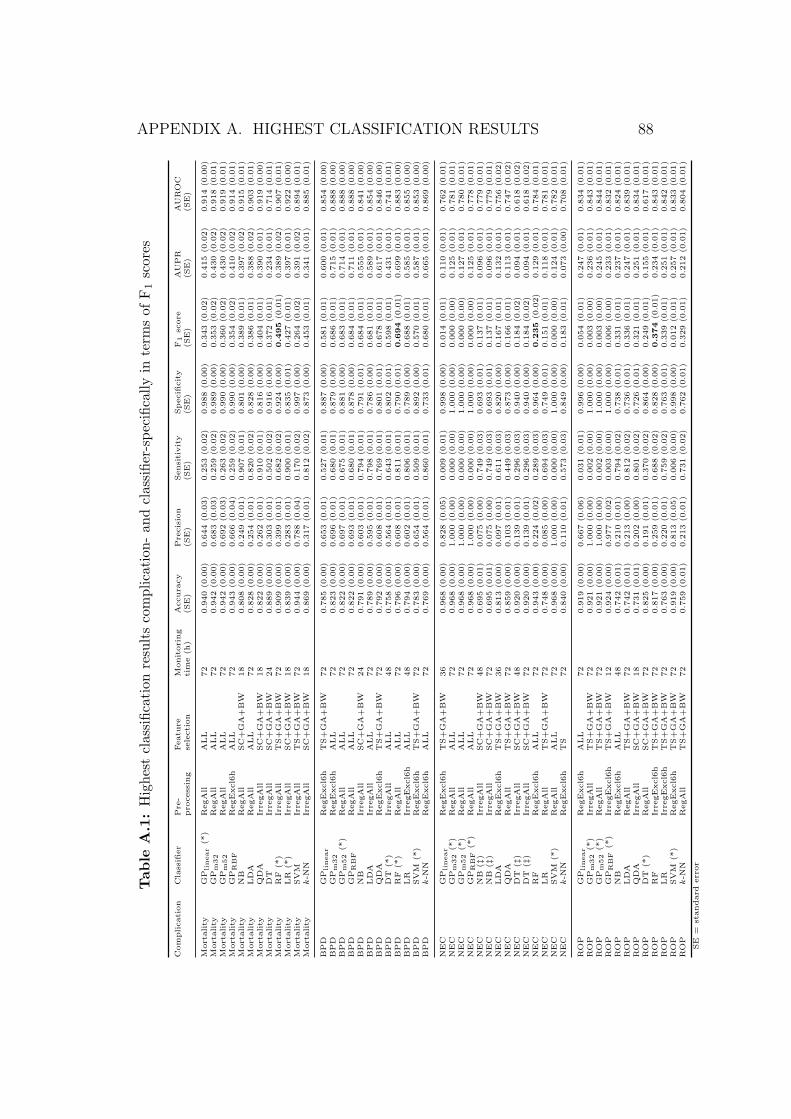
The results show large differences in the performance of classifiers. Randomforests, k-nearest neighbours, and logistic regression result in the highest F1

scores. The highest values of area under the precision-recall curve are achievedby random forests along with Gaussian processes. If area under the ROC curveis measured, random forests, Gaussian processes, and support vector machinesperform the best.

The monitored physiological parameters are time series and their sampling tech-nique can be altered. This shows only a negligible impact on the results. However,lengthening the monitoring time of physiological parameters to 36–48 hours hasa little but positive effect on the results. On the other hand, feature selectionhas a significant role: birth weight and gestational age are crucial for a highperformance. Further, combining them with other features improves the perfor-mance. For all that, the optimal data preprocessing procedure is classifier- andcomplication-specific.

Keywords: machine learning, binary classification, neonatal complica-tions, prediction

Language: English

ii

Aalto-yliopistoPerustieteiden korkeakouluLife science -teknologian koulutusohjelma

DIPLOMITYONTIIVISTELMA

Tekija: Janne Myllarinen

Tyon nimi:Dataan perustuva tapa ennustaa vastasyntyneiden laaketieteellisia diagnooseja

Paivays: 27.5.2018 Sivumaara: viii + 86

Paaaine: Monimutkaiset jarjestelmat Koodi: SCI3060

Valvoja: Prof. Simo Sarkka

Ohjaajat: TkT Jaakko HollmenFT Ali Bahrami Rad

Syntymapainoltaan hyvin pienet keskoset ovat suuressa riskissa kuolla tai saa-da hengenvaarallisia komplikaatioita alikehittyneisyyden takia. Naita vakavastisairaita vauvoja hoidetaan vastasyntyneiden teho-osastoilla, joissa heidan fysio-logista kuntoaan valvotaan jatkuvasti.

Tama tutkielma soveltaa koneoppimista valvottujen parametrien tallenteisiin jamuihin potilaskohtaisiin tietoihin, jotka on saatu HUS:n Lastenklinikalta. Tarkoi-tuksena on kayttaa binaarista luokittelua ennustamaan vastasyntyneiden kuollei-suutta ja kolmen sairauden puhkeamista. Nama sairaudet ovat bronkopulmonaa-linen dysplasia, nekrotisoiva enterokoliitti seka keskosten retionopatia. Suurin osanykyisesta tutkimuksesta on keskittynyt vertailemaan vain muutamia luokitteli-joita. Tassa tyossa vertaillaan siksi suurempaa maaraa eri luokittelualgoritme-ja. Yhden yleisesti kaytetyn mitan lisaksi ennusteita arvioidaan myos kahdellavahemman kaytetylla arviointimitalla: F1-arvolla ja tarkkuus–herkkyys-kayranalapuolisella alueella. Myos datan esikasittelyn ja piirteiden valinnan vaikutustaennustustulokseen tutkitaan.

Tulokset osoittavat suuria eroja eri luokittelijoiden valilla. Satunnaismetsilla, k-lahimman naapurin luokittimella seka logistisella regressiolla saadaan korkeim-mat F1-arvot. Suurimmat tarkkuus–herkkyys-kayran alapuoliset alueet saavute-tetaan satunnaismetsilla seka Gaussisten prosessien luokittimilla. Jos taas ROC-kayran alapuolinen alue mitataan, satunnaismetsat, Gaussisten prosessien luoki-tin ja tukivektorikoneet toimivat parhaiten.

Seuratut fysiologiset parametrit ovat aikasarjoja, joten niiden naytteenottotapaavoidaan muuttaa. Talla on vain pieni vaikutus tuloksiin. Fysiologisten para-metrien seuranta-ajan pidentamisella 36–48 tuntiin on kuitenkin pieni, muttamyonteinen vaikutus tuloksiin. Piirteiden valinnalla on puolestaan merkittavastivalia: syntymapaino ja gestaatioika ovat ratkaisevia hyvien tulosten saamiseksi.Niiden yhdistaminen muiden piirteiden kanssa parantaa tuloksia. Ihanteellinendatan esikasittely on kaikesta huolimatta luokittelija- ja komplikaatiokohtaista.

Asiasanat: koneoppiminen, binaarinen luokittelu, vastasyntyneidenkomplikaatiot, ennustaminen

Kieli: Englanti

iii

Acknowledgements

I would like to thank Professor Simo Sarkka for offering me this fascinatingMaster’s thesis position at the edge of data science and medical engineeringin the research group of Sensor Informatics and Medical Engineering and forsupervising my thesis. In addition, I want to thank my thesis advisors Dr.Jaakko Hollmen and Dr. Ali Bahrami Rad for valuable feedback and supportduring the thesis process.

I acknowledge Professor Sture Andersson and Dr. Markus Leskinen for in-troducing me to the world of neonatology, which I was not acquainted withbefore starting the thesis last autumn, and for valuable advice in medicinerelated matters. Furthermore, I would like to thank Dr. Olli-Pekka Rinta-Koski for all the practicalities, discussions about the data science in neona-tology, and the earlier work that founded an excellent basis for this Master’sthesis. I am also grateful to all the competent and splendid colleagues at myown and at the neighbouring research groups for the daily discussions.

And finally, I would like to thank my family and friends at home and abroadfor supporting me throughout the years.

Espoo, 27th May 2019

Janne Myllarinen

iv

Contents

Abstract ii

Tiivistelma iii

Acknowledgements iv

Contents v

Abbreviations and Acronyms vii

1 Introduction 1

2 Background 4

2.1 Neonatology . . . . . . . . . . . . . . . . . . . . . . . . . . . . 4

2.1.1 Neonatal infants . . . . . . . . . . . . . . . . . . . . . 42.1.2 Typical neonatal complications . . . . . . . . . . . . . 5

2.1.3 Evaluating the neonatal condition . . . . . . . . . . . . 6

2.1.4 Monitoring the neonatal physiological variables . . . . 7

2.2 Time series analysis . . . . . . . . . . . . . . . . . . . . . . . . 8

2.2.1 Time series . . . . . . . . . . . . . . . . . . . . . . . . 82.2.2 Feature extraction . . . . . . . . . . . . . . . . . . . . 92.2.3 Feature selection . . . . . . . . . . . . . . . . . . . . . 10

2.3 Machine learning classification methods . . . . . . . . . . . . . 10

2.3.1 Machine learning and classification in general . . . . . 10

2.3.2 Gaussian processes . . . . . . . . . . . . . . . . . . . . 12

2.3.3 Naıve Bayes . . . . . . . . . . . . . . . . . . . . . . . . 15

2.3.4 Linear discriminant analysis . . . . . . . . . . . . . . . 16

2.3.5 Quadratic discriminant analysis . . . . . . . . . . . . . 17

2.3.6 Decision trees . . . . . . . . . . . . . . . . . . . . . . . 172.3.7 Random forests . . . . . . . . . . . . . . . . . . . . . . 18

v

2.3.8 Logistic regression . . . . . . . . . . . . . . . . . . . . 19

2.3.9 Support vector machines . . . . . . . . . . . . . . . . . 19

2.3.10 k-nearest neighbours . . . . . . . . . . . . . . . . . . . 21

2.4 Evaluating classification results . . . . . . . . . . . . . . . . . 21

2.4.1 Performance measures . . . . . . . . . . . . . . . . . . 212.4.2 Applicability of measures . . . . . . . . . . . . . . . . . 25

2.5 Challenges in clinical data . . . . . . . . . . . . . . . . . . . . 26

2.6 Previous work . . . . . . . . . . . . . . . . . . . . . . . . . . . 292.6.1 Mortality predictions . . . . . . . . . . . . . . . . . . . 30

2.6.2 Morbidity predictions . . . . . . . . . . . . . . . . . . . 31

2.7 Background conclusions . . . . . . . . . . . . . . . . . . . . . 38

3 Materials and Methods 403.1 Data . . . . . . . . . . . . . . . . . . . . . . . . . . . . . . . . 40

3.1.1 Data collection and storing system . . . . . . . . . . . 40

3.1.2 Data description . . . . . . . . . . . . . . . . . . . . . 41

3.1.3 Data quality evaluation . . . . . . . . . . . . . . . . . . 43

3.2 Methods . . . . . . . . . . . . . . . . . . . . . . . . . . . . . . 453.2.1 Extracting time series . . . . . . . . . . . . . . . . . . 45

3.2.2 Preprocessing the data . . . . . . . . . . . . . . . . . . 46

3.2.3 Feature extraction and selection . . . . . . . . . . . . . 483.2.4 Implementation . . . . . . . . . . . . . . . . . . . . . . 49

4 Results 514.1 Optimal classification algorithms . . . . . . . . . . . . . . . . 51

4.1.1 Classifier and complication comparison . . . . . . . . . 51

4.1.2 Comparison to previous work . . . . . . . . . . . . . . 53

4.2 Optimal data preprocessing and feature selection . . . . . . . 57

4.2.1 Impact of time series preprocessing . . . . . . . . . . . 57

4.2.2 Impact of the length of the monitoring time . . . . . . 61

4.2.3 Impact of feature selection . . . . . . . . . . . . . . . . 66

5 Discussion 71

6 Conclusions 75

Bibliography 77

A Highest classification results 87

vi

Abbreviations and Acronyms

APACHE Acute Physiology And Chronic Health EvaluationAUPR Area under the precision-recall curveAUROC Area under the receiver operating characteristics

curveBPD Bronchopulmonary dysplasiaBW Birth weightconst constantCRIB Clinical Risk Index for BabiesDT Decision treeEHR Electronic health recordsELBW Extremely low birth weightFN False negativeFP False positiveFPR False positive rateGA Gestational ageGP Gaussian processHR Heart rateHRC Heart rate characteristicsICD International statistical classification of diseases and

related health problemsICU Intensive care unitIrregAll Irregular sampling, all hours includedIrregExcl6h Irregular sampling, first six hours of life excludedk-NN k-nearest neighboursLDA Linear discriminant analysisLOCF Last-observation-carry-forwardLR Logistic regressionm32 Matern kernel with ν = 3/2m52 Matern kernel with ν = 5/2MEWS Modified Early Warning Score

vii

MIMIC Multiparameter Intelligent Monitoring in IntensiveCare

NB Naıve BayesNEC Necrotising enterocolitisNICU Neonatal intensive care unitNTISS National Therapeutic Intervention Scoring SystemPAA Piecewise aggregate approximationPPV Positive predictive valuePR Precision-recallPRISM Paediatric Risk of MortalityQDA Quadratic discriminant analysisRBF Radial basis functionRegAll Regular sampling, all hours includedRegExcl6h Regular sampling, first six hours of life excludedRF Random forestROC Receiver operating characteristicsROP Retinopathy of prematuritySAPS Simplified Acute Physiology ScoreSE Standard errorSC Scores SNAP-II and SNAPPE-IISNAP Score for Neonatal Acute PhysiologySNAP-II Score for Neonatal Acute Physiology IISNAP-PE Score for Neonatal Acute Physiology – Perinatal Ex-

tensionSNAPPE-II Score for Neonatal Acute Physiology – Perinatal Ex-

tension IISOFA Sepsis-related Organ Failure AssessmentSpO2 Peripheral oxygen saturationSQL Structured query languageSVM Support vector machineTN True negativeTNR True negative rateTP True positiveTPR True positive rateTS Time seriesVLBW Very low birth weightVLGA Very low gestational age

viii

1

1. Introduction

Digitalisation of healthcare generates vast amounts of patient-specific med-ical data. At intensive care units (ICUs), they contain measurement valuesfrom patient monitoring, laboratory test results, and clinical notes writtenby doctors and nurses. These data enable opportunities for machine learningto discover knowledge (Meyfroidt et al., 2009). Various machine learningapproaches with various purposes have been proposed to analyse all types ofdata originated from human beings. They include, but are not limited to, bio-metric authentication from electroencephalogram signals (Haukipuro et al.,2019), prediction of morbidities associated with preterm birth from physi-ological parameter measurements (Saria et al., 2010), sequencing genomicdata (Libbrecht and Noble, 2015), detection of arrhythmia from electrocar-diogram recordings (Suotsalo and Sarkka, 2017), and segmentation of theanatomical regions of the brain from magnetic resonance images (de Brebissonand Montana, 2015).

Physiology of patients is monitored continuously during their stay at ICUwhich applies also to the smallest patients of all, the preterm infants, whichare taken care of at neonatal ICUs (NICUs). These patients are prone tolife-threatening complications of preterm birth that are a consequence oftheir bodies and vital functions not being as developed as those of terminfants (McGregor, 2013). Sadly, preterm birth is a major reason for theworldwide mortality of children under the age of five years (WHO and MCEE,2018). Fortunately, machine learning may provide a solution, or at least ahelp, when applied on the physiological parameter measurements and otherrelevant data of preterm infants. Machine learning algorithms may be utilisedat NICUs for predicting certain medical complications related to, for instance,respiratory system or sight (McGregor, 2013). Evidence for the applicabilityof machine learning on the neonatal health care exists. Among others, Fer-reira et al. (2012) diagnosed neonatal jaundice from a large number of health-related parameters, Temko et al. (2011) predicted neonatal seizures from elec-troencephalography data, and Rinta-Koski et al. (2017b, 2018) used several

CHAPTER 1. INTRODUCTION 2

physiological parameters and other information to predict a few prevalentneonatal morbidities as well as neonatal mortality.

Even though medical doctors are experts in their field, there is a need fordata-driven analyses if multiple physiological parameters affect concurrentlythe well-being and survival of infants. Humans are capable of analysing andrecognising patterns from data with three dimensions at most, but we arenot able to interpret accurately the data of higher dimensionality (Holzinger,2016). Accordingly, a computer – together with machine learning algorithmsand different types of medical data – is required to perform those analyses.Nonetheless, the intention is not to replace the doctors with algorithms butto provide them with real-time decision support tools. The tools can monitorthe patients and suspect potential complications in advance so that doctorscan evaluate these patients more carefully (Mani et al., 2014).

During 1999–2013, the NICU at Children’s Hospital, Helsinki University Hos-pital has been collecting and storing masses of data for more than 2,000preterm infant patients with a very low birth weight (VLBW). This numbercorresponds to around one-third of all Finnish VLBW infants born duringthose years. This database is exceptionally wide in terms of temporal scaleand coverage, also globally. A few studies, including Immeli et al. (2017)and Rinta-Koski et al. (2017b), have already utilised this database.

A decent amount of research has been conducted on predicting medical com-plications with machine learning algorithms. However, most of those studieshave repeatedly applied the same algorithms to make predictions, and theliterature is lacking their wider comparison. Therefore, the first researchobjective of this study is to determine which algorithms are the most suit-able for predicting neonatal complications and if there are differences in thepredictability of different complications. This is executed by applying 12 ma-chine learning algorithms on neonatal mortality and three morbidities, andby comparing their predictive capabilities.

Patient cohorts are often imbalanced, meaning the ratio of sick patients toall subjects is low. Due to the rareness of sick patients, identifying themis challenging from the machine learning point of view. If machine learningalgorithms are applied on imbalanced data and evaluated inappropriately,they tend to show misleading results. This is the case in many of the pre-vious studies. They evaluate the results using accuracy and area under thereceiver operating characteristics curve (see Section 2.4) and receive question-ably high results (Saito and Rehmsmeier, 2015; Rokach, 2010; Rollins et al.,2015; Libbrecht and Noble, 2015). Using incorrect measures can have fatalconsequences if the sick patients are not identified and given medical treat-

CHAPTER 1. INTRODUCTION 3

ment on time, but the measure still shows a high performance. Therefore,the second goal of this work is to present less-used measures that functionmore truthfully with imbalanced data. These measures and a more com-monly used measure are applied to evaluate the performance of machinelearning algorithms. Further, the results of this work are compared to previ-ous studies. Since making reliable comparisons between distinct datasets ischallenging (Salcedo-Bernal et al., 2016), the results are primarily comparedto studies that have been performed on the exactly same neonatal data fromthe NICU at Helsinki University Hospital.

As the high-quality database has a wide coverage of different types of patient-specific data, the third and more technical research objective of this work isto specify the optimal data preprocessing and feature selection technique forneonatal mortality and morbidity predictions. To be precise, the optimaltime series sampling of the temporal physiological parameters and the op-timal length of the monitoring time of the same parameters are examinedin the preprocessing phase. Moreover, including the most relevant featuresin the model can improve its prediction performance (Guyon and Elisseeff,2003). Therefore, the optimal combination of health-related parameters isstudied in the feature selection phase.

By finding the best machine learning algorithms, by assessing the results withappropriate evaluation criteria, and by determining the optimal preprocess-ing and feature selection procedure, the analysis tool could be implementedin real hospital environment some day. This decision support tool wouldassist medical doctors to plan the treat of the critically ill preterm infantsbefore the complications have occurred or their symptoms become too severe.Foremost, this would improve the care of the neonates, prevent them fromdeveloping critical and life-long complications, and save human lives.

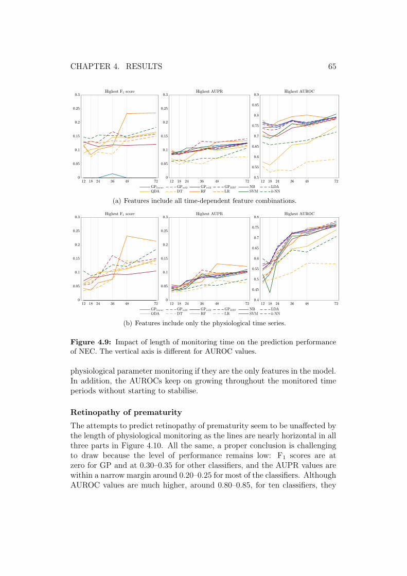
The work is structured as follows. Chapter 2 presents the theoretical back-ground, concentrating on data science, and a literature review consideringprevious studies. Chapter 3 describes the preterm infant data and themethodology how the data have been analysed, followed by the results inChapter 4. The results are interpreted and the research questions are an-swered in Chapter 5. Finally, Chapter 6 concludes the work.

4

2. Background

2.1 Neonatology

The term neonatology, a subspecialty of paediatrics, has been introduced forthe first time in 1960, and it focuses on the medical care and treatment ofhuman newborns, neonates (Avery et al., 2005). This section provides a briefintroduction to neonates, their medical complications, patient monitoring,and traditional scores to evaluate patients’ physical condition.

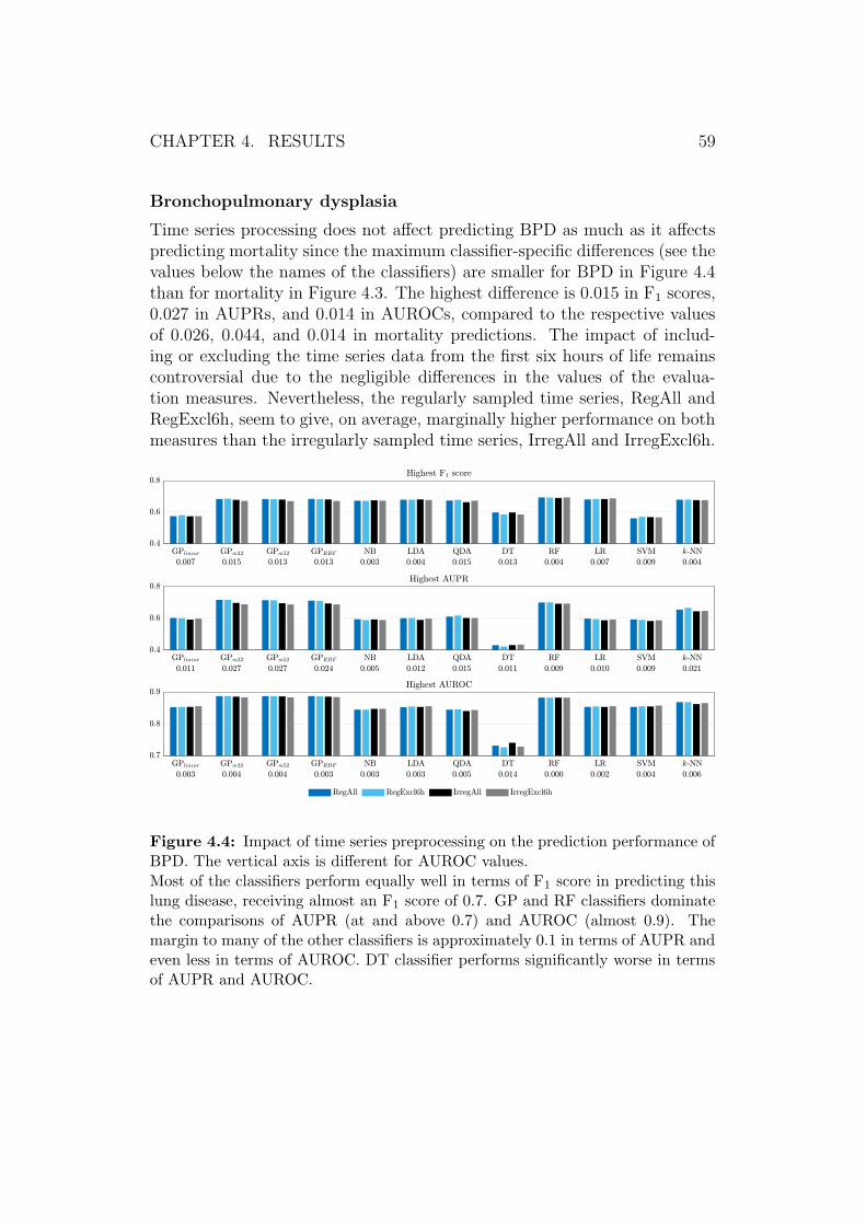
2.1.1 Neonatal infants

Neonates, which require critical care at neonatal intensive care units, are mostoften preterm infants, who are prone to numerous complications and illnessesdue to their underdeveloped organs and young age (McGregor, 2013; Averyet al., 2005). Approximately 15 million preterm infants are born worldwideannually, which corresponds to more than 10 % of all neonates, but this rate,however, varies country-specifically between 5 % and 18 % (WHO, 2018).

Gestational age (GA) and birth weight (BW) are important and widely usedattributes to describe neonates. GA means the time period from the first dayof the last normal menstrual period of the mother to the day of delivery, andGA is usually reported in weeks (American Academy of Pediatrics, 2004).If GA of a newborn is less than 32 weeks, the infant is said to have a verylow gestational age (VLGA) (Fattore et al., 2015). In addition, infants bornbefore the gestational age of 37 weeks are called preterm, between the 37th

and the 41st week are term, and after the 41st week are post term (Gomellaet al., 2013). Very low birth weight (VLBW) infants weigh less than 1500 g,and extremely low birth weight (ELBW) infants less than 1000 g (Averyet al., 2005; Gomella et al., 2013).

CHAPTER 2. BACKGROUND 5

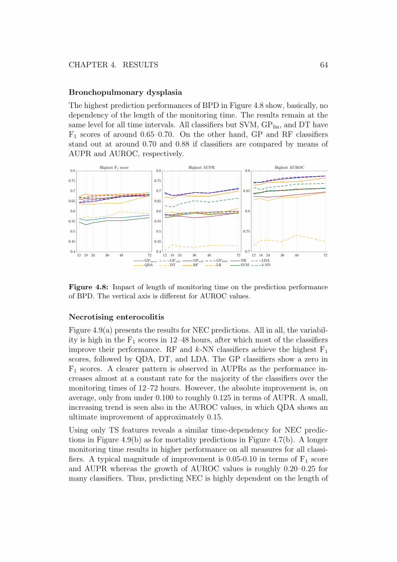
2.1.2 Typical neonatal complications

ELBW infants tend to have all kinds of health issues that can be respiratory(e.g., respiratory distress syndrome), cardiovascular (e.g., patent ductus ar-teriosus), central nervous system (e.g., intraventricular haemorrhage), renal(e.g., electrolyte imbalance), ophthalmologic (e.g., retinopathy of prematu-rity), gastrointestinal–nutritional (e.g., necrotising enterocolitis or jaundice),or immunologic (e.g., proneness to infections) problems (Avery et al., 2005).Critical care of VLBW and VLGA infants is costly, and according to Fattoreet al. (2015), the cost of saving one preterm infant from very likely death ise 20,000–e 40,000. In this study, neonatal mortality as well as bronchopul-monary dysplasia, necrotising enterocolitis, and retinopathy of prematurityare of a special interest.

Neonatal mortality has been on a decrease during the ongoing millenniumas Figure 2.1 presents (United Nations, 2019). Still, it corresponds to 2.5 mil-lion annual deaths globally (UNICEF et al., 2018). Complications of pretermbirth caused almost 0.9 million of all neonatal deaths, which also accountsfor approximately 6 % of all 15 million annually born preterm infants (WHOand MCEE, 2018; WHO, 2018). What is more, the mortality rate amongVLBW and VLGA infants is even higher. In Finland, it is 11.4 % one monthafter the birth and 11.7 % after one year (Fattore et al., 2015).

Figure 2.1: Neonatal mortality rate globally and in Finland during 2000–2017.Data from United Nations (2019).

Bronchopulmonary dysplasia (BPD) is a chronic lung disease, developedin preterm infants due to factors compromising normal development in theimmature lung, such as treatment of additional oxygen and the use of me-chanical ventilation (Avery et al., 2005). A low birth weight and gestationalage are associated with the risk of developing BPD (Gomella et al., 2013;


Wajs et al., 2006, 2007). Approximately 30 % of ELBW infants are diag-nosed with BPD (Gomella et al., 2013; Walsh et al., 2006).

Necrotising enterocolitis (NEC) is a disease of gastrointestinal tract ofpreterm neonates, where inflammation and bacterial invasion of the bowelwall leads to necrosis. Around 6 %–10 % of VLBW infants have NEC, andthe more preterm infants are at a higher risk of NEC (Gomella et al., 2013).

Retinopathy of prematurity (ROP) is a maldevelopment of the retinalvasculature, caused by interrupted retinal vessel formation, the symptoms ofwhich vary in severity and can lead to blindness at worst (Gomella et al.,2013). Supplementary oxygen given to infants is often believed to contributeto the development of ROP (Cirelli et al., 2013; Gomella et al., 2013). In ad-dition, a low birth weight correlates with the rate of developing ROP (Darlowet al., 2005). To prevent ROP, controlling and optimising the oxygen sat-uration of the patient is essential as well as maintaining the physiologicalstate of the patient stable to avoid infections, and thus, abnormal growthand development of the patient (Hellstrom et al., 2013).

2.1.3 Evaluating the neonatal condition

Throughout the years, several scoring systems have been introduced to nu-merically evaluate the condition of newborn infants. Demographic, physio-logical, and clinical data are used to calculate the scores, which give mortalityand different morbidities a quantification and are used to identify the high-risk patients (Dorling et al., 2005). Two types of scores exist: medical andstatistical. Medical experts have defined the parameters and their weightsused in medical scores, whereas the statistically relevant parameters havebeen selected for statistical scores (Dorling et al., 2005). The medical scoresare easier to be understood by the personnel using them, but their disadvan-tage is the worse performance in comparison to the statistical scores.

Multiple medical scores are discussed in the literature. National TherapeuticIntervention Scoring System, NTISS, is calculated from 62 values and usedto predict mortality and assess severity of illnesses (Gray et al., 1992). TheApgar score evaluates the neonatal condition from five signs (Apgar, 1953).The illness severity index and predictor of mortality Score for Neonatal AcutePhysiology, SNAP, is calculated from 34 values for VLBW infants (Richard-son et al., 1993a). Its extension, Score for Neonatal Acute Physiology – Peri-natal Extension, SNAP-PE, is calculated from SNAP and three additionalvalues using logistic regression (Richardson et al., 1993b).


Statistical techniques have been applied to select the parameters for the sim-plified versions of SNAP and SNAP-PE, namely SNAP-II and SNAPPE-II (Richardson et al., 2001). SNAP-II is calculated from six values andSNAPPE-II from SNAP-II and three additional values, which are similarto those of SNAP-PE (Richardson et al., 2001).

Logistic regression has been used to define the parameters for several sta-tistical scores. Clinical Risk Index for Babies, CRIB, predicts mortality forVLBW infants or infants with GA of less than 31 weeks from six values (In-ternational Neonatal Network, 1993). Its simplified version, CRIB II, is cal-culated from five redefined values for neonates with GA of 32 weeks (Parryet al., 2003). Berlin score (Maier et al., 1997) uses five values to assess themortality risk of VLBW patients.

Additionally, many other scores exist, and they evaluate the condition of childand adult patients. They include, but are not limited to, Acute PhysiologyAnd Chronic Health Evaluation, APACHE, (Knaus et al., 1981) along withthe revised versions APACHE II (Knaus et al., 1985), APACHE III (Knauset al., 1991), and APACHE IV (Zimmerman et al., 2006), Glasgow ComaScore (Teasdale and Jennett, 1974), Modified Early Warning Score, MEWS,(Subbe et al., 2001), Pediatric Risk of Mortality, PRISM, (Pollack et al.,1988) with its revised version PRISM III (Pollack et al., 1996), SimplifiedAcute Physiology Score, SAPS, (Le Gall et al., 1984) and its revised versionSAPS II (Le Gall et al., 1993) as well as Sepsis-related Organ Failure Assess-ment, SOFA, (Vincent et al., 1996) and quickSOFA (Singer et al., 2016).

Even though certain scores are widely adopted and used for research pur-poses, a single score cannot explain the true condition of an infant as theyalways emphasise some aspects over others (Dorling et al., 2005). The use ofscores has also been criticised as they are static values, calculated at singletime points only, and are not updated over time (Ghassemi et al., 2015).Therefore, continuous patient monitoring is essential in gaining correct in-formation about the condition of the patients.

2.1.4 Monitoring the neonatal physiological variables

The human physiology is monitored with various sensors to have an updatedview on the patient’s condition so that potential onset of medical compli-cations can be prevented by intervening them in advance (Murkovic et al.,2003). At NICUs, the infants are kept in incubators, where the temperatureand humidity conditions are appropriate. What is more, multiple functional-ities are integrated into incubators which can be medical care devices, such as


ventilators, or patient monitoring devices, such as pulse oximetry. The moni-tored parameters usually include, but are not limited to, electrocardiography,electroencephalography, heart rate (HR), blood pressure, temperature, res-piratory rate, and peripheral blood oxygen saturation (SpO2) (Rinta-Koski,2018; Murkovic et al., 2003).

The measurements quantify the state of preterm infant patients, which is arequirement for machine learning applications. Thus, the measurements formthe integral basis for this study since the continuous parameter monitoringenables to evaluate and model the patient’s condition with machine learningalgorithms instead of static scores.

2.2 Time series analysis

This section introduces time series and describes how information can be ex-tracted from them. Furthermore, techniques to identify the relevant featuresfrom all possible features are discussed in Section 2.2.3.

2.2.1 Time series

A time series consists of multiple consecutive observations of a parameter,measured over a certain time period (Batal et al., 2009). Each observationhas a value and a corresponding time stamp. If multiple parameters aremeasured simultaneously, the time series is called multivariate.

Similar temporal patterns are searched from physiological time series as theymay correspond to certain clinical diagnoses (Lehman et al., 2008). Con-sequently, the appearance of these patterns can reveal upcoming compli-cations before the condition of the patient deteriorates. Using time seriesand more complex temporal information may improve the prediction perfor-mance. Temporal patterns may include information that is not visible from asingle value; relationships between certain parameters and medication intakecan contain more information than only the newest monitored parametervalues (Batal et al., 2009).


2.2.2 Feature extraction

Feature extraction means finding the essential information from, potentially,massive amounts of data usually by reducing the dimensionality of the dataand by compressing the data into features (Duda et al., 2001). Based on thefeatures, dissimilar data can be distinguished from each other. Time seriesfeatures include, for example, regression slopes in certain intervals, maxi-mum transient increase and decrease of the values, and similarity measureswithin and between signals, of which autocorrelation coefficients measure thewithin-signal similarity and cross correlation coefficients the between-signalsimilarity (Lehman et al., 2008). Autoregressive–moving-average parameters,introduced by Wold (1938), are also a technique to extract information fromtime series.

Temporal abstraction patterns can be extracted from time series data usingfour methods as follows (Batal et al., 2012).

1. Temporal abstractions transform raw, multivariate time series data intoa symbolic form where information is encoded to a higher abstractionlevel (Moskovitch and Shahar, 2015). They are divided into two meth-ods:

(a) value or state abstractions categorise values to groups, such aslow, normal, and high, and

(b) trend abstractions categorise time intervals of predefined lengthto groups, such as increasing, steady, and decreasing (Batal et al.,2009; Sacchi et al., 2007).

2. Multivariate state sequences observe the value abstraction sequencesover time for multiple time series.

3. Temporal relations are based on Allen’s temporal logic (Allen, 1984),and they observe the timing of the occurrence of certain events, forexample, consecutive occurrences, or partly or totally overlapping oc-currences.

4. Temporal patterns observe the sequence of temporal relations.

Shapelets are another technique to extract information from time series.They are defined as exceptionally representative subsequences of the class,in which the whole time series belongs to (Ye and Keogh, 2009). In otherwords, shapelets find the relevant parts of time series that include enoughinformation to classify the whole time series. One more algorithm to identifytemporal patterns is segmented time series feature mine (Batal et al., 2009),which is based on the Apriori algorithm by Agrawal and Srikant (1994).


2.2.3 Feature selection

The number of extractable features is enormous. In feature selection, thenumber of extracted features is reduced so that only the most relevant onesare used in classification (Murphy, 2012). This improves the performance ofthe prediction, makes the computation more efficient, and explains what isessential in the underlying data (Guyon and Elisseeff, 2003; Salcedo-Bernalet al., 2016). However, Temko et al. (2011) prefer including all availablefeatures for support vector machine classification (see Section 2.3.9) sincethe presence of redundant features does not distract the classifier, unlike thelack of important features. As an acknowledgement, a variable, which doesnot improve the classification result alone, can improve it together with othervariables (Guyon and Elisseeff, 2003).

Three common feature selection techniques are filter, wrapper, and embed-ded methods, for which the reader is advised to refer to Guyon and Elisseeff(2003). Filter methods, such as the correlation criterion of the square ofPearson correlation coefficient, are suitable for binary classification. For in-stance, features with the lowest correlation with the outcome variable can beomitted from the model, which, however, may simultaneously decrease theclassification result (Salcedo-Bernal et al., 2016). Wrapper methods applythe machine learning algorithm of interest to identify the optimal features.They either select, as in forward selection, or omit, as in backward elimina-tion, the features one by one, ending up to a locally optimal performance.Embedded methods are a combination of filter and wrapper methods that canimprove the results in comparison to filter methods, but the improvement isnot guaranteed to be significant.

2.3 Machine learning classification methods

This section presents the principles of machine learning with a focus on de-scribing how classifiers determine the class for data points.

2.3.1 Machine learning and classification in general

A high-level division of machine learning is supervised and unsupervisedlearning (Hastie et al., 2001; Goodfellow et al., 2016; Murphy, 2012). Thegoal in both of them is to build a model that discovers knowledge fromdata, which are split into training data and test data. The training data


consist of input-output pairs D = {(x(i), y(i))}Ni=1, where N is the numberof observations (also called as data points, data instances, or cases), each of

which is required to have d known features x(i) = (x(i)1 , . . . , x

(i)d ) (also called

as attributes, predictive attributes, or explanatory variables) and one possiblyknown outcome variable y(i) (also called as class, label, target, or responsevariable) (Bellazzi and Zupan, 2008; Hastie et al., 2001; Goodfellow et al.,2016; Murphy, 2012; Bishop, 2006).

In supervised learning, the known features X = (x(1), . . . ,x(N))T and theknown outcome variables y = (y(1), . . . , y(N))T of the training data are usedto build a model. The purpose of the model is to predict the unknownoutcome variable y of unseen data instance of test data from their knownfeatures x by estimating the probability p(y |x) (Lucas, 2004; Hastie et al.,2001; Goodfellow et al., 2016). If the outcome variable can only have discretevalues or is qualitative, the machine learning problem is called classification,whereas a continuous outcome variable implies regression (Meyfroidt et al.,2009; Hastie et al., 2001).

In unsupervised learning, on the other hand, the outcome variables y areunknown, and the aim is to observe the features in the unlabeled dataD = {(x(i))}Ni=1 to learn the probability distribution p(x) (Murphy, 2012).The model is build by finding certain patterns in the attributes, based onwhich certain data points are grouped or clustered together (Meyfroidt et al.,2009). In addition to clustering, unsupervised learning covers, for example,association rules and self-organising maps (Hastie et al., 2001).

In the ICU context, an interesting question is to predict the survival of pa-tients, which can be implemented as a supervised binary classification prob-lem (Meyfroidt et al., 2009). In classification, the purpose is to build a modelbased on the training data, and then generalise the model on unseen datainstances. The features of an unseen data point x are used to assign thedata point with a label y ∈ {C1, . . . , CK} that represents one of K discreteclasses Ck, where k = 1, . . . , K (Bishop, 2006). The classes are separated bydecision boundaries, also known as decision surfaces, from each other in thefeature space.

In this work, the data instances are NICU patients and the input data con-sist of their physiological parameter measurements and other patient-specificinformation. Furthermore, the outcome variable y(i) ∈ {0, 1}, where y(i) = 0denotes the class C1, the patient i dies or is given a certain diagnosis, andy(i) = 1 denotes the class C2, the patient i does not die or is not given thediagnosis.

The generalisation capability is measured by generalisation error, test error


or classification error, which means the probability to misclassify an unseendata instance from the test data (Goodfellow et al., 2016; Rokach, 2010).Additionally, the machine learning models are evaluated with training errorswhich are errors due to misclassification, calculated from the training set.Minimising the training error means optimising the parameters of the modelfor the training set so accurately that the generalisation capability of themodel is reduced (Goodfellow et al., 2016). Thus, the test error increases,which is referred to as overfitting. It is one of the major challenges in machinelearning.

In the field of medicine, the most widely used machine learning classifiersinclude decision trees, random forests, artificial neural networks, Bayesiannetworks, support vector machines, and Gaussian processes, and there is noevidence that a certain classifier would be more suitable for a certain taskthan any other (Meyfroidt et al., 2009). Therefore, a variety of classifiers areapplied and compared to determine the most suitable classifiers for neonatalcomplication predictions to respond to the first research objective of thiswork.

2.3.2 Gaussian processes

Gaussian processes (GPs) are generalisations of the Gaussian probability dis-tribution, and they belong to probabilistic classification methods that pro-duce probabilities of belonging to a class instead of bare class labels (Bishop,2006; Rasmussen and Williams, 2006). The goal of Gaussian processes is tolearn the distribution over function for the given data p(f |X,y), and thendetermine the posterior or predictive probability p(y∗ |X,y,x∗) to predictthe label y∗ for a test data point x∗ (Rasmussen and Williams, 2006; Mur-phy, 2012). An example of GP classification result is presented in Figure 2.2.Next, binary GP classification is described in more detail, and the test datapoint is denoted with an asterisk (∗) for clarity.

First, a Gaussian process prior is adapted over a latent function f ∗ =(f(x(1)), . . . , f(x(N)), f(x∗)), which is defined as in Equation (2.1),

p(f ∗) = N (f ∗ |0,Σ∗), (2.1)

where the covariance matrix Σ∗ consists of elements Σ(x,x′) = k(x,x′),in which k(x,x′) is any positive semidefinite kernel function (Bishop, 2006;Murphy, 2012). For a test data point, the distribution of this latent variablef ∗ is defined by Rasmussen and Williams (2006) as in Equation (2.2),


ℛ2

HR

SpO2

0

0 %

200

100 %

0 200

0.50

0.25

0.750.50

0.50

0.25

ℛ1

ℛ2

ℛ1

Figure 2.2: A possible result of a GP classification based on two features: heartrate (HR) and peripheral oxygen saturation (SpO2). The left part shows thelocations of the data points of the blue and orange classes, and the right part showsthe contour plots for the predictive probabilities, where the black line representsthe decision boundary between decision regions R1 (blue class) and R2 (orangeclass). Figure following Rasmussen and Williams (2006).

p(f ∗ |X,y,x∗) = p(f ∗ |X,y,f) p(f |X,y) df . (2.2)

Second, a logistic sigmoid function σ(f ∗) = (1 + exp(f ∗))−1 is applied onthe latent to transform the result from the whole span of the x-axis into theinterval of [0, 1] to receive an appropriate binary classification result (Bishop,2006; Rasmussen and Williams, 2006).

Third, it is sufficient to calculate the posterior distribution only for one classp(y∗ = 1 |X,y,x∗) since the posterior distribution for the other class issimply its complement p(y∗ = 0 |X,y,x∗) = 1 − p(y∗ = 1 |X,y,x∗). Fol-lowing Bishop (2006) and Rasmussen and Williams (2006), the probabilisticprediction is calculated as a combination of the previous steps as in Equa-tion (2.3),

p(y∗ = 1 |X,y, f ∗) =

∫σ(f ∗) p(f ∗ |X,y,x∗) df ∗. (2.3)


Kernel functions for Gaussian processes

The choice of the covariance matrix or kernel function Σ is essential in GPclassification since assumptions of the similarities between data points areencoded in that (Rasmussen and Williams, 2006). Different kernels include,but are not limited to, constant, linear, squared exponential or radial ba-sis function (RBF), and Matern kernels in Equations (2.4a), (2.4b), (2.4c),and (2.4d), respectively,

kconst(x,x′) = σ2, (2.4a)

klinear(x,x′) = xTΣx′, (2.4b)

kRBF(x,x′) = exp(− r2

2`2), (2.4c)

and

kMatern(x,x′) =1

2ν−1Γ(ν)

(√2ν

`r

)ν

Kν

(√2ν

`r

), (2.4d)

where x and x′ are a pair of inputs, σ2 is a variance, r = x − x′ is astationary covariance function, ` is a characteristic length-scale, ν is a positiveparameter, Kν is a modified Bessel function (see Abramowitz and Stegun(1965)), and Γ is the gamma function (Rasmussen and Williams, 2006;Murphy, 2012). According to Rasmussen and Williams (2006), the mostinteresting Matern kernels from the machine learning perspective are the oneswith parameters ν = 3/2 and ν = 5/2 as in Equations (2.4e), and (2.4f),

kMatern32(x,x′) =

(1 +

√3r

`

)exp

(−√

3r

`

), (2.4e)

and

kMatern52(x,x′) =

(1 +

√5r

`+

5r2

3`2

)exp

(−√

5r

`

), (2.4f)

respectively.

Valid kernels can be constructed from other valid kernels by following simplerules (Bishop, 2006). For example, a sum or a product of two valid kernelsresults in a valid kernel (Rasmussen and Williams, 2006). In this work, four


distinct kernels are applied, and they correspond to the kernels of Rinta-Koski et al. (2018). These kernels are sums of linear, constant, and kernel-specifically optionally one of the kernels presented above, and the constructedkernels are as in Equations (2.5a), (2.5b), (2.5c), and (2.5d),

k1(x,x′) = klinear(x,x′) + kconst(x,x

′), (2.5a)


′) + kMatern32(x,x′), (2.5b)


′) + kMatern52(x,x′), (2.5c)

and


′) + kRBF(x,x′). (2.5d)

2.3.3 Naıve Bayes

The naıve Bayes classification (NB) is based on the Bayes formula in Equa-tion (2.6),

P (y = Ck |x) =p(x |Ck)P (Ck)

p(x), (2.6)

where Ck represents the kth class label, and the posterior probability P (y =Ck |x) for an unknown data instance x is calculated from likelihood p(x |Ck),prior probability P (Ck), and evidence p(x) (Duda et al., 2001; Mitchell,1997).

The goal of the naıve Bayes classifier is to calculate the maximum posteriorprobability, and thereby, classify the unseen data point to the most likelyclass (Duda et al., 2001). Additionally, the denominator in Equation (2.6)is irrelevant under the assumption of conditionally independent features xj,and it is omitted. The formula simplifies to Equation (2.7),

P (y = Ck |x) = argmaxCk ∈K

P (Ck)d∏j=1

p(xj |Ck), (2.7)

where d is the dimensionality of the feature vector x. Additional data in-stances contribute positively to the performance of the model as they makethe posterior probability density function sharper (Duda et al., 2001).


2.3.4 Linear discriminant analysis

Linear discriminant analysis (LDA) divides the d-dimensional space Rd intoclasses by hyperplanes whose decision boundaries are linear (Hastie et al.,2001). The decision boundary divides the feature space into two subspaces ordecision regions R1 for y = 0 and R2 for y = 1 in binary classification (Dudaet al., 2001). An example of binary LDA classification is in Figure 2.3(a).

LDA models the class conditional densities as Gaussian distributions as inEquation (2.8),

p(x | y = Ck,θ) = N (x |µk,Σk), (2.8)

where θ refers to the parameters of the model: the d-dimensional, class-specific mean vector µk, and the class-specific covariance matrix Σk (Mur-phy, 2012). LDA assumes that all classes have a common covariance ma-trix (Hastie et al., 2001; Murphy, 2012). Thus, the class-specific covariancematrices simplify to a common covariance matrix as Σk = Σ ∀k. The poste-rior probabilities for class labels are formulated as in Equation (2.9),

p(y = Ck |x,θ) = xTΣ−1µk −1

2µTkΣ−1µk + log πk, (2.9)

where πk denotes the class-specific prior probability P (Ck) (Hastie et al.,2001; Murphy, 2012).

ℛ1

ℛ2

(a) Binary LDA classification with thelinear decision boundary

ℛ1

ℛ2

(b) Binary QDA classification with thequadratic decision boundary

Figure 2.3: Two binary discriminant analysis classifiers separate the blue andorange classes. Figure modified from Murphy (2012).


2.3.5 Quadratic discriminant analysis

The linear decision boundaries of LDA (see Section 2.3.4) are not always ad-equate to separate the classes from each other, and in those cases, quadraticdiscriminant analysis (QDA) might result in a better classification. QDA hasquadratic decision boundaries instead of linear, and the class-specific covari-ance matrices are not assumed to be equal (Hastie et al., 2001). Thus, eachclass Ck has its own covariance matrix Σk. Quadratic discriminant functionsare formulated as in Equation (2.10),

p(y = Ck |x,θ) = −1

2log |Σk| −

1

2(x− µk)TΣ−1

k (x− µk) + log πk, (2.10)

(Hastie et al., 2001). A possible classification of QDA is presented in Fig-ure 2.3(b).

2.3.6 Decision trees

Classification and regression trees have been introduced by Breiman et al.(1984), who recognised their applicability to medical diagnosis predictions.In decision trees (DT), thresholds are set for the feature values, and eachthreshold splits the data into two non-overlapping subsets R1 and R2 atdecision points (Breiman et al., 1984; Goodfellow et al., 2016; Murphy, 2012).Figure 2.4(a) presents the tree-like structure of DT. More mathematically,the decision points divide the feature space into regions with hyperplanes,resulting in hyper-rectangles that correspond to the leaf nodes (Podgorelecet al., 2002). Rectangle regions R1 and R2 are illustrated in Figure 2.4(b).

Splitting the data into smaller subsets is repeated until almost all data in-stances of the subsets or leaf nodes belong to the same class Ck (Goodfellowet al., 2016; Duda et al., 2001). Had all data instances in a leaf node thesame outcome variable, the model could be overfitting (Podgorelec et al.,2002). Overfitting is prevented by pruning, in which the number of splits islimited (Murphy, 2012). To test the performance of a decision tree, the fea-tures of a new data instance are compared to the thresholds in the tree-likestructure, and the label of the leaf node becomes the class of the test datainstance.

The advantage of decision trees is the easily understandable rules (Mani et al.,2014; Duda et al., 2001). Decision trees accept both continuous and discretedata as input (Murphy, 2012). They are also relatively robust classifiers to


HR ≤ 160

𝑌𝑒𝑠 𝑁𝑜

SpO2 ≤ 60% ℛ1


HR ≤ 40 ℛ2


ℛ1 ℛ2

(a) The logic of a decision tree with deci-sion points (ellipses) and leaf nodes (rect-angles)

HR

ℛ1

SpO2

0

0 %

40 160

60 %

ℛ1

ℛ2

ℛ2

(b) The same decision tree as regions infeature space

Figure 2.4: A possible result of a decision tree of two features: heart rate (HR)and peripheral oxygen saturation (SpO2).

labelling errors, and outliers (Meyfroidt et al., 2009; Murphy, 2012). Thedisadvantages of decision trees include their poor performance on incompletedata, the lack of alternative solutions as they are able to produce only onemodel for a given problem, and their incapability to emphasise the moreimportant decisions over the less important ones (Podgorelec et al., 2002).

2.3.7 Random forests

Random forests (RF) consist of an ensemble of trees, each of which hasbeen trained with a slightly dissimilar subset of the training data (Murphy,2012; Meyfroidt et al., 2009). The sampling of the subsets is independentand identically distributed, resulting in slightly dissimilar trees for each sam-pling (Breiman, 2001). After the trees are grown, their results are averagedor the most common result is voted to be the result of RF model. Accord-ingly, the model has a lower variance than single decision trees. The numberof trees in the forest is not relevant as the generalisation error of the modelconverges as long as there are sufficiently many trees (Breiman, 2001).


2.3.8 Logistic regression

Despite its name, logistic regression (LR) is a classification method, whoseorigin lays in linear regression (Bishop, 2006; Goodfellow et al., 2016). Lo-gistic regression models the posterior probabilities of the perfectly separableclasses with linear functions (Hastie et al., 2001). The regression coefficientsor weights w of the functions do not have a closed-form solution but theyare optimised with algorithms such as maximum likelihood estimation orgradient descent (Murphy, 2012). Logistic regression is presented in Equa-tion (2.11),

p(y = Ck |x,W ) =exp(wT

kx)K∑i=1

exp(wTi x)

, (2.11)

where W contains all the class-specific weight vectors wk, and K is thenumber of classes Ck (Murphy, 2012).

2.3.9 Support vector machines

Support vector machines (SVMs) are generalisations of logistic regressionsince perfect linear separability of the classes is not required (Hastie et al.,2001). Moreover, SVMs output only the class labels, not the probabilities asLR does (Goodfellow et al., 2016).

SVMs are based on mapping the input data into a high-dimensional featurespace where the optimal linear decision boundaries or hyperplanes are setbetween the classes, so that the margin between the vectors of the classesis maximised (Cortes and Vapnik, 1995). Mathematically, maximising themargin equals to minimising the weight vector ‖w‖2, since the margin equalsto 2‖w‖ (Cortes and Vapnik, 1995; Hastie et al., 2001; Bishop, 2006). Thus,

the optimisation problem is as in Equation (2.12),

minw,b

1

2‖w‖2

subject to y(i)(wTφ(x(i)) + b) ≥ 1, i = 1, . . . , N,

(2.12)

where φ denotes the fixed feature-space mapping, and b the bias parameter.Weight vectors w, for which y(i)(wTφ(x(i)) + b) equals to 1 or −1 lie at themaximum margin hyperplanes and are support vectors. SVM separates the


classes so that one class has a positive value for wTφ(x(i)) + b and negativefor the other (Bishop, 2006; Goodfellow et al., 2016).

Since the perfect linear separability is not required for the classes in SVMclassification, some of the observations are let to be misclassified on theincorrect side of the decision boundary. Therefore, slack variables ξ(i) ≥ 0are introduced. Equation (2.13) updates the the optimisation problem andthe constraints,

minw,b

1

2‖w‖2 + γ

N∑i=1

ξ(i)

subject to y(i)(wTφ(x(i)) + b) ≥ 1− ξ(i), i = 1, . . . , N

ξ(i) ≥ 0, i = 1, . . . , N,

(2.13)

where∑N

i=1 ξ(i) sets an upper bound for the number of misclassified data

points, and thus, γ > 0 is a constant controlling the split between the marginand the slack variable penalty (Cortes and Vapnik, 1995; Hastie et al., 2001;Bishop, 2006). If ξ(i) = 0, the data point i has a correct classification as itlies at the margin or on its correct side. 0 < ξ(i) ≤ 1 means also a correctclassification, but the data point lies inside the margin but on the correct sideof the decision boundary. A data point with ξ(i) > 1 is misclassified since itlies on the incorrect side of the decision boundary. Binary SVM classificationwith slack variables is shown in Figure 2.5.

𝑚𝑎𝑟𝑔𝑖𝑛ℛ1

ℛ2

ξ(𝑖) < 1

ξ(𝑖) = 0

1

𝒘

ξ(𝑖) > 1

𝒘𝑇𝝓 𝒙 𝑖 + 𝑏 = 0

𝒘𝑇𝝓 𝒙 𝑖 + 𝑏 = −1

𝒘𝑇𝝓 𝒙 𝑖 + 𝑏 = 1

Figure 2.5: The black decision boundary divides the space into regions R1 andR2, leaving a margin between the classes in binary SVM classification. Figurefollowing Hastie et al. (2001) and Murphy (2012).


2.3.10 k-nearest neighbours

In k-nearest neighbours classification (k-NN), a data instance is classifiedto the same class as the majority of its k closest neighbours, and k =1, . . . , N (Bishop, 2006; Hastie et al., 2001; Duda et al., 2001; Mitchell, 1997).If an equal number of neighbours belongs to different classes, the class can beselected, for example, randomly between them. The selected distance mea-sure, such as Euclidean, Mahalanobis, or Manhattan distance, may affect theclassification result (Duda et al., 2001). Since k-NN is a non-parametric algo-rithm, the underlying data are allowed to have any distribution (Goodfellowet al., 2016).

2.4 Evaluating classification results

Measures evaluate and enable to compare the performance of distinct clas-sifiers and the performance of the same classifier with any changes in pa-rameters, features, or other factors (Marsland, 2015). This section providesbackground for achieving the second research goal of this work by introducingperformance measures and by assessing their usability in classification.

2.4.1 Performance measures

Many of the classifiers, presented in Section 2.3, do not provide a pre-dicted label but probabilities in the interval of 0.00–1.00 of belonging toclasses (Fawcett, 2006). This probability has to exceed a predefined thresh-old so that a data point is assigned with a corresponding label. Thereby, thechoice of the threshold affects the labelling, and thus, the results. However,the correct threshold varies application-specifically, and selecting the correctone is not straightforward (Saito and Rehmsmeier, 2015). Therefore, single-threshold and threshold-free measures are presented next. For a detailedexplanation of the measures, the reader is advised to refer to Sokolova andLapalme (2009) and Saito and Rehmsmeier (2015).

Confusion matrix is a simple matrix of classification results, and it formsa foundation for classification evaluation. Confusion matrix, presented inTable 2.1, has a size of 2× 2 in binary classification. The four sections in theconfusion matrix represent how a data point can be classified.

• True positive (TP ) means a data point, which belongs to class C1

and is classified to belong to C1.


Table 2.1: Confusion matrix used in binary classification.

Predicted class

Positive (C1) Negative (C2)

True classPositive (C1) True positive (TP ) False negative (FN)

Negative (C2) False positive (FP ) True negative (TN)

• False negative (FN) means a data point, which belongs to class C1

but is classified not to belong to C1.

• False positive (FP ) means a data point, which does not belong toclass C1 but is classified to belong to C1.

• True negative (TN) means a data point, which does not belong toclass C1 and is classified not to belong to C1.

Single-threshold measures

The following measures require a threshold for the probability of belongingto a class to assess the classification performance. Altering the thresholdchanges also the number of the four outcomes (TP , FN , FP , TN), andaccordingly, the following performance measures (Van Trees, 1968).

Accuracy is the rate of classifying the data instances into the correct classesas defined in Equation (2.14).

Accuracy =TP + TN

TP + FN + FP + TN(2.14)

Precision or positive predictive value (PPV) is the rate of data instanceswith a positive classification, for which the classification is correct as definedin Equation (2.15). In the NICU context, precision means the rate of patientswith a complication diagnosis who are truly unwell. A low precision impliesthat more patients are suspected to have a complication than have that inreality, which means playing it safe in the practical sense.

Precision =TP

TP + FP(2.15)

Sensitivity, recall, or true positive rate (TPR) is the rate of data instancesbelonging to the positive class which are classified correctly as defined in


Equation (2.16). Thus, sensitivity measures the rate of identifying the un-well patients from all unwell patients, which is vital from the medical pointof view. Not identifying an unwell patient can have critical consequences,and therefore, false positives are much more acceptable than false nega-tives (Rollins et al., 2015).

Sensitivity =TP

TP + FN(2.16)

Specificity or true negative rate (TNR) is the rate of data instances belong-ing to the negative class which are classified correctly as defined in Equa-tion (2.17). Thereby, specificity measures the rate of truly healthy patients,which have been diagnosed as healthy.

Specificity =TN

FP + TN(2.17)

False positive rate (FPR) is the rate of data instances belonging to thenegative class which are classified incorrectly as defined in Equation (2.18).At NICUs, FPR is the rate of healthy patients, which are diagnosed as sick.

False positive rate = 1− specifity =FP

FP + TN(2.18)

F1 score, F-score, or F-measure, defined in Equation (2.19), is the harmonicmean of precision and sensitivity.

F1 score =2 · precision · sensitivity

precision + sensitivity(2.19)

Threshold-free measures

The following measures merge single-threshold measures so that all possiblethresholds in the range of 0.00–1.00 are taken into account.

Receiver operating characteristics (ROC), example in Figure 2.6(a), vi-sualise the results of a binary classification task (Hanley and McNeil, 1982;Fawcett, 2006). The false positive rates (FPRs) for all thresholds lie onthe x-axis, and they are plotted against the true positive rates (TPRs) for allthresholds on the y-axis (Van Trees, 1968; Fawcett, 2006; Davis and Goadrich,2006; Saito and Rehmsmeier, 2015). The ROC curve of a perfect classifica-tion passes from (0,0) through (0,1) to (1,1). Random guessing produces a


diagonal ROC curve, from left bottom corner to right top corner. Therefore,only classifiers in the upper left triangle outperform random guessing.

Area under the ROC curve (abbreviated as AUROC in this work) is asingle value between 0 and 1, which makes comparing ROC curves of distinctclassifiers more convenient (Hanley and McNeil, 1982; Saito and Rehmsmeier,2015; Fawcett, 2006). If AUROC is 1, the two groups have been identifiedperfectly and they are totally distinct whereas an AUROC value of 0.5 impli-cates random guessing and the groups have not been identified at all (Fawcett,2006; Swets, 1988; Griffin and Moorman, 2001). Thus, all classifiers shouldhave an AUROC higher than 0.5. Noteworthy, AUROC quantifies only thearea, not the shape of the curve, and two distinct ROC curves can have thesame AUROC.

(a) ROC curves (b) PR curves

Figure 2.6: Results for seven classifiers in terms of ROC and PR curves.

Precision-recall (PR) curve is another classification performance measure,illustrated in Figure 2.6(b). The values of recall for all thresholds lie on thex-axis, and they are plotted against the values of precision for all thresholdson the y-axis (Davis and Goadrich, 2006; Saito and Rehmsmeier, 2015). Theperfect classification lies in the upper right corner.

Area under the PR curve (abbreviated as AUPR in this work) quanti-fies the PR curve into a single value between 0 and 1, making comparisonsbetween classifiers more convenient.


2.4.2 Applicability of measures

Since the classification results can be assessed with many measures, the choiceof the measure depends on what is wanted to be measured. Thereby, thechoice is also a matter of opinion. The different measures emphasise differentaspects as described in Section 2.4.1. However, only appropriate evaluationcriteria provide justified results that answer to research questions. Therefore,it is essential to be aware of the capabilities and limitations of different mea-sures (Fawcett, 2006). For example in complication predictions, the interestis often in identifying the sick patients among all patients, which means clas-sifying the positive class correctly. Therefore, the most suitable measures arerequired to concentrate on evaluating that.

The suitability of measures for assessing the classification performance de-pends partly also on the underlying data. Data imbalance (see Section 2.5)means that the ratio of the positive and negative classes is not equal, formingmajority and minority classes. This disproportion affects the choice of theappropriate measure. For example, accuracy is not the optimal evaluationcriterion for imbalanced datasets if the task is to identify the minority classrepresentatives (Libbrecht and Noble, 2015; Marsland, 2015; Rollins et al.,2015; Rokach, 2010). If the sick patients were the minority class and thehealthy patients the majority class, classifying all patients to the class of thehealthy would result in a high accuracy even though none of the sick patientswas identified and classified correctly. Therefore, the use of other measuresis required, and Marsland (2015) expresses that either the pair of precisionand recall or the pair of specificity and sensitivity provides more informationthan accuracy alone.

In medical data, the class of sick subjects is often the minority class. Accord-ingly, class imbalance has to be considered in medicine since misclassifyingsick patients as healthy can be vital for them if they do not receive medicalcare on time (Weiss and Provost, 2001). Therefore, it is important to identifyall sick patients, which implies that a high sensitivity is appreciated. Eventhough misclassifying healthy patients as sick is not harmful for them, it iswaste of resources to consider and treat them as risk patients in vain. There-fore, it is essential to classify only the sick patients as sick, which implicatesthat a high precision is valuable. In accordance, precision and sensitivity aremore appropriate evaluation criteria than accuracy (Sun et al., 2009).

The single-threshold measure F1 score is a derivative of precision and sen-sitivity, and using F1 score is supported from the data imbalance point ofview (Marsland, 2015; Sun et al., 2009). F1 score evaluates the ability of


the classifier to truly identify the data points of the underrepresented class,and it does not provide overly optimistic results either as accuracy and someother measures do. The same applies to the threshold-free AUPR that isanother derivative of precision and sensitivity (recall).

Saito and Rehmsmeier (2015) researched the performance of ROC and PRcurves on balanced and imbalanced datasets, concluding PR curves result inmore informative and intuitive plots if data imbalance is present. However,this is debatable since Fawcett (2006) encourages the use of ROC curvesover PR curves due to their resistance to changes in class balance. For allthat, according to Saito and Rehmsmeier (2015), ROC curves are used morefrequently in the studies, and the statement is supported by the findings inSection 2.6. Only a few researchers have reported other measures: Rollinset al. (2015) have reported F1 score and Desautels et al. (2016) AUPR.

2.5 Challenges in clinical data

Hogan and Wagner (1997) describe the data quality with two measures: cor-rectness is the proportion of truly correct data observations to incorrect dataobservations, and completeness is the proportion of recorded observations toall recordable observations. Both correctness and completeness are importantfactors regarding the performance of machine learning algorithms. Generallyspeaking, medical data and physiological parameter recordings are seldomtotally correct or complete. The data are sparse and noisy, the samplingis irregular, and the data samples are plagued by human error (Ghassemiet al., 2015; Marlin et al., 2012). Additionally, some values may be out ofrange, and there can be gaps in the time series (Salcedo-Bernal et al., 2016).Additionally, some of the missing values are caused by probe dropouts suchas malfunctions or removals of the measuring equipment (Stanculescu et al.,2014a). Consequently, all these decrease the correctness and completeness ofthe data.

Missing values

Missing values mean gaps in the data or the sparsity of the data. They in-crease the level of incompleteness of the data, which is characteristic for manyreal-world data sets (Donders et al., 2006; Kotsiantis et al., 2006). Sometimespreprocessing the data produces missing values. For example, Lehman et al.(2008) replaced measurement values out of range by missing values, but filledthem later by interpolation.


While statistical methods function well with data that contain noise andmissing values, predictive methods often fail with such data. Therefore, manytechniques have been developed to deal with missing values. Saar-Tsechanskyand Provost (2007) suggest four alternative approaches to handle missingvalues as follows.

1. The whole data instance (x(i), y(i)) with a missing value is discarded.

2. The whole feature xj with a missing value is discarded.

3. The missing value x(i)j is acquired.

4. The missing value x(i)j is estimated by

(a) replacing it with the mean or mode of the feature j,

(b) replacing it with an arbitrary unique value, or

(c) calculating it from the distribution of the feature j.

To extend suggestion 4(a), multiple extrapolation methods have been pro-posed to fill the missing values by, for example, with the mean of the wholedata or the mean of the adjacent values (Meyfroidt et al., 2009). Further-more, a simple last-observation-carry-forward (LOCF) method has been ap-plied (Desautels et al., 2016; Overall et al., 2009; Mani et al., 2014). InLOCF, missing values are replaced with the previous known value.

In addition, more sophisticated and complex methods have been proposed.The generative probabilistic models, such as autoregressive hidden Markovmodels, are appropriate for estimating missing values as they utilise marginal-isation (Stanculescu et al., 2014b). Marginalisation means drawing probabil-ities for unknown values from the known values, and the direct dependenciesbetween all values are taken into account. However, these models requirethe proportion of missing values to be relatively small. Further, generalisedlinear mixed models can be applied on sparse data as they function despitethe missing values (Overall et al., 2009). Still, the use of simpler models isadvised due to their better performance.

Irregular sampling

Irregular sampling means that the time intervals between samples do not stayconstant. This irregularity causes many modelling methods to fail, which can,however, be tackled by making assumptions about the functional form of thedata (Ghassemi et al., 2015). Of course, making assumptions introduces newbias to the model.

A technique to tackle the varying sampling frequency is piecewise aggregateapproximation (PAA), in which the time series are cut into time frames ofequal length (Keogh et al., 2001). Then, the values in each time frame are


averaged for each time frame. In cases where no values exist in the frame,the same value is selected as in the previous or the following frame (Salcedo-Bernal et al., 2016). Marlin et al. (2012) applied PAA with one-hour-longintervals and mean filtering but they also pointed out the issue of potentialinformation loss. Despite not calling it PAA, Lehman et al. (2008) used asimilar approach with one-minute-long time intervals where medians of thesamples were calculated for each minute, and Lehman et al. (2015) had thesame interval length but calculated averages.

A time series can also be translated into a string of symbols to avoid thechallenges, caused by irregularly sampled time series. One symbolic methodis symbolic aggregate approximation (Lin et al., 2007). First, this methoduses PAA to split the time series into frames of equal length, each of whichis assigned with the mean value of that frame. Then, the mean values arediscretised by setting breakpoints B for their values, which are used to as-sign each time frame with a symbol such as an alphabet. For example, twobreakpoints B = {β1, β2}, β1 < β2, are set for a PAA representation. Valuesbelow β1 are given an A, the values between β1 and β2 a B, and the valuesabove β2 a C. The breakpoints B are advised to be derived from the Gaussiandistribution (Lin et al., 2007).

Ghassemi et al. (2015) proposed a time series modelling method to make pre-dictions from clinical data. Their method uses multiple irregularly sampledtime series along with their between and within correlations. This multi-variate method introduces a new latent space and uses the multi-task GPmodels, outperforming univariate time series methods.

Imbalanced data

Class imbalance means the disproportional occurrence of class representativesin the data, leading to majority and minority classes. Imbalanced data areproblematic especially in binary classification if the class of interest is theminority class (Cerqueira et al., 2014). As the model has not been trainedwith a sufficient number of minority class representatives, many classifiers failin classifying the minority class correctly (Weiss and Provost, 2001; Marsland,2015). In these cases, the classifier does not necessarily learn – or is even nottrained with – all possible variations of the minority class representatives.

The class imbalance can be managed with resampling. In oversampling, theminority class samples are copied at random until their number has increasedclose to the number of the majority class samples, and in the opposite case,in undersampling, the majority class samples are removed at random untiltheir number has decreased close to the number of the minority class sam-


ples (Japkowicz and Stephen, 2002; Estabrooks et al., 2004). There is nounambiguous solution which resampling technique to use since their perfor-mance depends on the underlying data (Estabrooks et al., 2004). Select-ing either often improves the result compared to using the imbalanced data.Nevertheless, Japkowicz and Stephen (2002) conclude that oversampling out-performs undersampling.

Improving the data quality with expert knowledge

Besides knowledge of data science, substance knowledge is required to se-lect the most important features for the machine learning algorithms at thedata preprocessing phase (Cerqueira et al., 2014). Adding expert or back-ground knowledge in machine learning has also been considered so that themachine learning models would not depend only on the input data but alsoon the clinical expertise (Lucas, 2004; Bellazzi and Zupan, 2008). Holzinger(2016) discusses the possibility to create interactive machine learning algo-rithms, where an expert is involved in the actual learning phase of machinelearning algorithms, in addition to the preprocessing phase. Nonetheless, this“human-in-the-loop” approach lacks quantitative research on its performanceand suitability in health care and medicine.

Comparability

Salcedo-Bernal et al. (2016) point out the difficulty to compare the resultsof different research papers in the clinical field since the applied data andparameters vary from paper to paper, thus making it hard to conclude whichmodel gives the most accurate predictions. Recently, the open MIMIC II(Multiparameter Intelligent Monitoring in Intensive Care) database (Saeedet al., 2011), available on Physionet (Goldberger et al., 2000), has been usedby several researchers, such as Salcedo-Bernal et al. (2016), Lehman et al.(2015), Ghassemi et al. (2015), and Calvert et al. (2016).

2.6 Previous work

The results of a comprehensive literature review to the previous work ofmachine learning applications in neonatology, at ICUs, and in health care ingeneral are provided in this section. The common denominator for all thestudies presented here is the data-based approach to predict mortality or amedical complication.


2.6.1 Mortality predictions

Neonatal mortality has been studied with GP and SVM classifiers usingmeasurements from five physiological time series, GA, BW, and SNAP-IIand SNAPPE-II scores (Rinta-Koski et al., 2017a, 2018). Rinta-Koski et al.(2017a) studied the impact of feature selection of 24-hour-long time series us-ing GP with the kernel presented in Equation (2.5d). They showed the high-est AUROC to be 0.94 with many different feature combinations. Selectingonly the time series features decreased the result slightly to 0.88. Rinta-Koskiet al. (2018) extended the research to cover also time series of other lengths,and they included SVM classifier and GP classifiers with other kernels inEquations (2.5a), (2.5b), and (2.5c) in the study. As a result, GP classifiersoutperformed SVM, and the optimal length of the monitoring time was 48hours from the birth. Similarly to Rinta-Koski et al. (2017a), different fea-ture combinations were tested. If only time series features were used, theyshowed an AUROC of 0.926. That remains lower than 0.947 or 0.949, whichwere achieved by combining time series features with GA and BW, or GA,BW, and the medical scores SNAP-II and SNAPPE-II, respectively.

Neonatal mortality was also studied by Cerqueira et al. (2014) who, first, ap-plied statistical analyses and medical experts to select the preferred featuresfor the model. Majority of the features were single values, such as binaryindicators of the presence of a certain complication or the occurrence of acertain treatment. Then, they applied SVM and artificial neural networksto predict the death of patients and achieved AUROCs of 0.83 and 0.84,respectively.

Salcedo-Bernal et al. (2016) predicted the in-hospital mortality at an ICUusing multivariate time series of heart rate, respiratory rate, and SpO2. Theycompared LR, neural networks, k-NN, and DT classifiers and received accu-racies of 0.68, 0.75, 0.65, and 0.74, respectively. Optimising the parametersof the models did not improve the results in logistic regression and neuralnetworks.

Lehman et al. (2015) utilised time series of heart rate and blood pressure aswell as the medical scores APACHE III, APACHE IV, and SAPS to predictin-hospital mortality of ICU patients with a switching vector autoregressiveframework (Murphy, 1998; Nemati et al., 2012). The highest results arereceived by selecting blood pressure along with one of the scores at a timeas features. Blood pressure alone results in an AUROC of 0.70, while SAPSincreases it to 0.77 (SAPS alone 0.65), APACHE III to 0.84 (APACHE IIIalone 0.80), and APACHE IV to 0.85 (APACHE IV alone 0.82).


Ramon et al. (2007) predicted the mortality at an ICU from a large datasetwhich contain, among others, the patient basic information, physiologicalparameter measurements, and medication details. The classification perfor-mance was measured with AUROC, which was 0.79 for DT, 0.82 for firstorder RF, 0.88 for NB, and 0.86 for tree augmented NB. They also pre-dicted a number of different complications, concluding RF classifiers alwaysoutperform DTs.

In addition to supervised learning, unsupervised machine learning can beapplied to identify the patients in danger to die. Marlin et al. (2012) stud-ied mortality in ICU environment using clustering and mainly physiologicalparameter measurements. They resulted in an AUROC of approximately0.85–0.90. The performance was improved if the length of parameter moni-toring was prolonged.

In addition to the aforementioned mortality research, many other studieshave been conducted. The reader is advised to refer to Medlock et al. (2011)who have made a comprehensive review of existing studies on the predictionmodels of mortality, focusing solely on VLBW and VLGA infants. Thenumber of the identified studies is 41 and the majority of them, 35 to beaccurate, have used logistic regression to predict mortality.

2.6.2 Morbidity predictions

Besides predicting morbidities in general, predicting neonatal morbiditieshas been in the interest of a decent amount of research. These morbiditiesinclude, but are not limited to, BPD, NEC, ROP, and sepsis. In the early2000s, the focus was on identifying the most relevant features that are eithercapable of detecting or predicting a certain morbidity. The features wereusually selected among the patient basic information, such as GA or thepresence of a certain complication. In the recent years, numerous machinelearning approaches have been proposed to predict morbidities from varioustypes of data, including monitored sensor values or laboratory test results.

Saria et al. (2010) predicted BPD, intraventricular haemorrhage, NEC, ROP,and death from GA, BW, and the physiological parameters of heart rate,respiratory rate, and oxygen saturation with Bayesian modelling. Predictingany of the aforementioned morbidities or death, they achieved an AUROCof 0.92. The medical scores Apgar, CRIB, SNAP-II, and SNAPPE-II aloneresulted in 0.70, 0.85, 0.83, and 0.88 respectively. They also compared theperformance of their method and the medical scores for infections, such asNEC, sepsis, and urinary tract infection, and cardiopulmonary complications,


such as BPD, resulting in AUROCs of 0.97 and 0.98 compared to 0.74 and0.72, 0.90 and 0.91, 0.84 and 0.86, and 0.91 and 0.93 for Apgar, CRIB,SNAP-II, and SNAPPE-II scores, respectively. Their final observation wasthat including all features in the model shows a higher AUROC of 0.91compared to including only GA and BW (AUROC 0.85) or only physiologicalparameters (AUROC 0.85).

Rinta-Koski et al. (2017b) predicted BPD, NEC, and ROP with a GP clas-sifier using the mean and standard deviation of five physiological time seriesas well as GA, BW, and SNAP-II and SNAPPE-II scores. They also studiedthe effect of feature selection on the results. They were able to achieve anAUROC of 0.87 for BPD. Even though AUROCs were 0.74 and 0.84 for NECand ROP, respectively, predicting them was not successful as the sensitivitieswere close to zero.

Bronchopulmonary dysplasia

The previous research has predicted neonatal BPD from a variety of featuresthat have mainly been patient basic information or indicators of the presenceof a certain complication or treatment. However, the use of physiological timeseries as features is limited. In contrary, many classifiers have been appliedto study which classifier is the most suitable to predict BPD. Nevertheless,no general consensus exists for the optimal classifier even though majority ofthe research has focused on logistic regression and some papers apply neuralnetworks or SVMs (Ochab and Wajs, 2016).

Wajs et al. (2006) used BW, a binary variable of the presence of respiratorysupport, alveolar-arterial ratio, a binary variable of the presence of patentductus arteriosus, SpO2, and heart rate as features in logistic regression topredict neonatal BPD. They received an AUROC of 0.942.

Furthermore, Wajs et al. (2007) examined all possible combinations of 14 fea-tures. The optimal features consisted of BW, a binary variable of the presenceof patent ductus arteriosus, surfactant administration, a binary variable ofthe presence of respiratory support, ratio of time when SpO2 is below 85 %,mean heart rate, and the ratio of mean SpO2 during the first week to meanSpO2 during the first day. LR and RBF neural network were applied on thesefeatures, resulting in AUROCs of 0.91 and 0.95, respectively.

Ochab and Wajs (2014b) compared various combinations of the same 14features, and predicted BPD with both SVM and LR, both implemented inMatlab. Despite the feature combination, LR outperformed SVMs in termsof accuracy and sensitivity. Interestingly, the implementation environmentaffected the results since Ochab and Wajs (2014a) repeated the experiments


with the LIBSVM library by Chang and Lin (2011). This time, SVM was ableto achieve a better accuracy and sensitivity for certain feature combinationsthan LR, outperforming usually also the Matlab implementation of SVM.Furthermore, Ochab and Wajs (2016) studied the feature selection for thesame task using LIBSVM and LR classifiers. They drew a conclusion thatLR provides a higher accuracy when the number of features is less thanseven, whereas LIBSVM functions better when more than seven features areincluded. Finally, Wajs et al. (2018) predicted BPD from the same featuresusing NB classifier which was outperformed by either LR or SVM, dependingon the performance measure.

Multiple studies have applied logistic regression and other statistical methodsto identify the features associated with neonatal BPD. These studies, how-ever, have seldom used physiological time series as features but rather staticvalues. Bhering et al. (2007) used four variables, which include GA and thepresence of mechanical ventilation, and received an AUROC of 0.935. Cunhaet al. (2005) found eight features, such as BW, GA, and presence of patentductus arteriosus, to be associated with a developing BPD. Romagnoli et al.(1998) used similar features and showed an AUROC of 0.960 for infants atthe age of 72 hours. Kim et al. (2005) used GA, BW, Apgar score and fiveother features to predict BPD, resulting in AUROCs of 0.90, 0.91, and 0.94at the ages of four, seven, and ten days, respectively.

Using not only LR but also tree models, Ambalavanan et al. (2008) were ableto associate lower BW, higher oxygen concentration, male gender, additionalsurfactant doses, higher oxygenation index, and outborn status with a higherrisk of BPD and death. However, they acknowledged that more validation isrequired due to the limited number of patients in the study.

Laughon et al. (2011) compared the effect of feature selection on the classifica-tion performance and discovered that six optimal features are GA, BW, raceand ethnicity, sex, respiratory support, fraction of inspired oxygen. Thesefeatures resulted in AUROCs of 0.793 and 0.854 at the first and the 28th dayof life, respectively.

Necrotising enterocolitis

The research to predict NEC with machine learning algorithms is limited,but a few applications are able to distinguish patients with NEC from thosewithout as well as the required treatment, surgical or medical. In fact, nobiological indicator of NEC is currently used in practise due to their lowpredictive power (Sylvester et al., 2014). Therefore, the current practisediagnoses NEC clinically instead of diagnostic tests (Ji et al., 2014).


Since NEC and sepsis have similar pathophysiologic features, Stone et al.(2013) used a successful technique to predict sepsis, namely heart rate charac-teristics (HRC) index, and extended it to NEC predictions felicitously. Stoneet al. (2013) observed that the baseline of HRC index rises for the patientsrequiring a surgical intervention, and the rise appears for 1–3 days prior tothe NEC diagnosis. Additionally, a significant increase in the HRC index isdetected for 16 hours prior to the diagnosis of surgical NEC and for 6 hoursprior to that of medical NEC.

Sylvester et al. (2014) investigated if it was possible to predict the treatmenttype, surgical or medical, beforehand from clinical parameters or biomarkers.Using 27 clinical input features for LDA, the algorithm distinguishes the twotypes with an AUROC of 0.817, whereas three specific biomarkers show ahigher AUROC of 0.856. Were the clinical parameters and biomarkers usedtogether, the treatment groups are distinguished perfectly. The statisticallymost significant parameters in the analysis were male gender and BW.

Ji et al. (2014) used the same 27 clinical parameters as Sylvester et al. (2014)and applied LDA to predict the level of risk for NEC using three categories:low, intermediate, and high. This prediction received an AUROC of 0.85.

Retinopathy of prematurity

Approaches to predict ROP mainly use retinal images or basic patient infor-mation as input. In addition, statistical research has been conducted to selectthe most predictive and revealing features of ROP. Unfortunately, continuousphysiological measurements as the input data lack research.

Bolon-Canedo et al. (2015b) performed a comprehensive study on the usabil-ity of machine learning in predicting ROP from retinal images. First, theycompared six feature selection algorithms, all of which produced similar re-sults. Second, they compared these features to features which were selectedby a group of experts. Similarities in these two feature sets were remarkable.Third, they performed binary classification of the patients using DT, NB,k-NN, SVM, and compared the results to the classification made by the ex-perts. The algorithms achieved at least as good results as the experts. Thelowest classification errors (less than 0.11) were achieved by NB and SVM.However, developing a golden standard for the process of predicting ROP isdifficult, which this study did not reach either.

Ataer-Cansizoglu et al. (2015) used Gaussian mixture model to extract fea-tures from retinal images and used SVM to classify patients. They receivedan accuracy of 0.95 which approximately equals to the accuracy of classifi-cation made by experts. Also, Bolon-Canedo et al. (2015a) used Gaussian


mixture model to extract features from retinal images. They combined thosefeatures with traditional statistical features, and used DT, NB, SVM, andRF for classification. SVM achieved the highest accuracy of 0.911 when allfeatures were included in the model, whereas the features from Gaussianmixture model alone had an accuracy of 0.905. Furthermore, various im-age analysis approaches have been proposed to detect the patients at risk ofROP (Wittenberg et al., 2012).

Rollins et al. (2015) proposed a discrete conditional phase-type model thatfunctions with class imbalance. The model requires a classifiers as a compo-nent in the model. SVM component was shown to outperform DT and RFcomponents when ROP was predicted for VLGA and VLBW infants. Theyachieved an F1 score of 0.738.

Rather than machine learning, Lofqvist et al. (2006) used logistic regressionto select the features for ROP predictions. The optimal features are postnatalweight gain, insulin-like growth factor level, and insulin-like growth factorbinding protein 3 level, all measured on a weekly basis. Further, Wu et al.(2012) simplified the algorithm to include only the weekly weight gain andwere still able to predict ROP.

Binenbaum et al. (2011) used LR to observe that BW, GA, and postna-tal weight gain provide the highest prediction performance for the risk ofROP. Darlow et al. (2005) performed statistical analyses and LR to definethe most significant variables for ROP predictions. They were able to asso-ciate a low GA, a low BW among other preterm infants with the same GA,and the male gender with an increased risk of developing ROP.

Sepsis

Sepsis causes sudden clinical deterioration of neonates and is a major rea-son behind neonatal morbidities and mortality (Griffin and Moorman, 2001;Griffin et al., 2003). Therefore, detecting sepsis as early as possible is im-portant so that more aggressive and targeted treatment can be started ontime (Desautels et al., 2016). However, diagnosing sepsis from clinical signsand laboratory tests beforehand has been proven to be difficult (Escobar,1999; Griffin and Moorman, 2001). To make more reliable diagnoses forsepsis, several studies have been conducted on the heart rate characteristics(HRC) and their abnormalities, such as reduced variability and transient de-celerations (Griffin and Moorman, 2001; Kovatchev et al., 2003; Griffin et al.,2003, 2004, 2005; Moorman et al., 2006). Furthermore, the most appropriatefeatures for a predictive model have been identified from physiological timeseries and laboratory test results. Machine learning and statistical mod-


els have been used to predict neonatal sepsis and sepsis in general, and thepredictive results have been compared to predictions of medical scores (Stan-culescu et al., 2014a,b; Calvert et al., 2016; Desautels et al., 2016; Mani et al.,2014; Wang et al., 2013).

Griffin and Moorman (2001) examined the relationship between HRC, such asits statistical moments and percentiles, and the risk of neonatal sepsis usingmultivariate logistic regression. The explanatory power of scores SNAP andNTISS on the occurrence of sepsis was also studied. They observed thatHRC are abnormal for 24 hours prior to the clinical suspicion of sepsis withan AUROC of 0.90 – especially skewness and percentiles revealed the patientsat risk. As sepsis deteriorates the physiological parameters of the patients,there is a rise in both SNAP and NTISS scores before the sepsis suspicion.SNAP is affected significantly more than NTISS. What is more, the infantswith sepsis tend to have a BW of approximately 200 g less and a GA ofapproximately two weeks less than healthy infants.

To have more evidence for the results, Griffin et al. (2003) showed that thereis a significant connection (AUROC 0.75) between HRC index and neona-tal sepsis and other sepsis-like illnesses. Further, Griffin et al. (2004) usedmultivariate logistic regression to show that HRC index had an associationwith death up to seven days in advance (the highest AUROC of 0.74) andthe cumulative HRC index was associated with in-hospital mortality (AU-ROC of 0.83). In addition, using HRC index together with BW, GA, andpostnatal age in a multivariate logistic regression was shown to increase thepredictive power of sepsis: AUROC increased from 0.75 to 0.77 while the ad-ditional features result in 0.67 alone Griffin et al. (2003). Also, the AUROCof death predictions increased from 0.74 to 0.85 with the additional features,which resulted in 0.70 alone (Griffin et al., 2004). However, combining theparameters with the cumulative HRC index for predicting in-hospital mor-tality reduced the AUROC from 0.83 to 0.79. The parameters alone hadan AUROC of 0.76. Additionally, Griffin et al. (2005) combined HRC indexwith certain laboratory test results, which improved the AUROC of neonatalsepsis predictions from 0.73 to 0.82. Laboratory tests alone resulted to anAUROC of 0.75.

Kovatchev et al. (2003) studied sample asymmetries of heart rate variabilityin order to detect neonatal sepsis or systemic inflammatory response syn-drome. Their results showed the sample asymmetries grow before the diag-nosis and treatment of the complication.

Calvert et al. (2016) used machine learning algorithms to predict sepsis ofICU patients from the following physiological time series: systolic blood pres-


sure, pulse pressure, heart rate, temperature, respiration rate, white bloodcell count, pH, blood oxygen saturation, and age. They were able to reachan AUROC of 0.92 at three hours before a systemic inflammatory responsesyndrome period, and an AUROC of 0.83 at less than three hours before thatperiod.

Desautels et al. (2016) predicted sepsis of ICU patients from eight physiologi-cal time series: systolic blood pressure, pulse pressure, heart rate, respirationrate, temperature, peripheral capillary oxygen saturation, age, and Glasgowcoma score. They applied binary classification on the patients, receiving anAUROC of 0.88 and an AUPR of 0.60 at the sepsis onset. This result out-performed the performance of multiple other medical scores, which were 0.80and 0.33 for MEWS, 0.70 and 0.23 for SAPS II, 0.61 and 0.16 for systemicinflammatory response syndrome by Bone et al. (1992), 0.73 and 0.28 forSOFA, and 0.77 and 0.28 for quickSOFA in terms of AUROC and AUPR,respectively. Differences between the scores were explained by the differentinput data requirements. The algorithm functioned well also with sparsedata where up to 60 % of the data were missing.

Mani et al. (2014) compared many classifiers to predict neonatal sepsis. Theclassifiers were tested on data both including and excluding the culture neg-ative sepsis patients, receiving the following AUROCs for the two datasets:RF (0.57, 0.65), classification and regression trees (0.65, 0.77), SVM (0.61,0.68), k-NN (0.54, 0.62), LR (0.61, 0.61), lazy Bayesian rules (0.62, 0.58),NB (0.64, 0.78), and tree augmented naıve Bayes (0.59, 0.53). All classifiershad higher specificity than predictions made by physicians, and almost allclassifiers also exceeded the sensitivity of the experts’ predictions.

Wang et al. (2013) used embedded methods in feature selection to identifythe optimal biomarkers from ten alternatives, such as white blood cell countand haemoglobin count, to predict neonatal sepsis. They applied canonicalcorrelation analysis to identify the optimal features and sparse support vectormachine classifier to test their predictive power. The highest accuracy of0.875 was achieved with five features.

Also unsupervised learning has been applied to predict sepsis. Based on thefactorial switching linear dynamical system by Quinn et al. (2009), Stan-culescu et al. (2014a) developed a deep learning styled hierarchical switchinglinear dynamical system which takes the complex interactions of a dynamicsystem into account. They used time series of heart rate and SpO2 measure-ments to predict sepsis of VLBW infants since lowered heart rate and SpO2

are often indicators of sepsis. They resulted in an AUROC of 0.69.

To have a comparison for the results of Stanculescu et al. (2014a), Stanculescu


et al. (2014b) performed the same analysis on the same time series to predictsepsis, but this time using a few additional measurements and autoregressivehidden Markov models. They received an AUROC of 0.74 when all data wereused and an AUROC of 0.72 without any missing values.

2.7 Background conclusions

The Section 2.1 discusses the need for research in the field of neonatologywhere the preterm infant patients are prone to critical morbidities and mor-tality. Their lives may be saved if the occurrence of the morbidities or deathcan be predicted in advance as it enables more time for the medical doctorsto treat them. Therefore, conducting this study is important, and the othersections in Chapter 2 present topics that are relevant in order to achieve thethree research objectives of this study.

The first research objective is to identify the most suitable classifiers forpredicting neonatal mortality and morbidities, and thus, 12 classifiers arepresented in Section 2.3. However, Meyfroidt et al. (2009) concluded that noclassifier is more suitable than any other, and Ochab and Wajs (2016) statedthat no model has been generally accepted for predicting BPD. Currently, LRhas been applied the most widely in this field as Section 2.6 and Medlock et al.(2011) reveal, followed by SVM and DT classifiers. QDA is the only algorithmof the presented classifiers that lacks research. Based on the previous studies,it is difficult to compare the performance of different classifiers and name themost suitable classifier due to the dissimilar underlying data (Salcedo-Bernalet al., 2016). Therefore, this study compares the performance of the 12classifiers on the same data.

What comes to the predictability of complications, the literature review inSection 2.6 shows successful proposals in predicting mortality and BPD fromvarying types of patient data. The mortality predictions have achieved AU-ROCs of 0.88 with NB, 0.83 with SVM, 0.82 with RF, 0.79 and 0.74 with DT,0.68 with LR, and 0.65 with k-NN. Previous BPD predictions have, on theother hand, reached high AUROCs with logistic regression that are 0.94 and0.91. There is less research on predicting NEC and ROP, and the results aremore modest. No indicator has been proven to be powerful enough to predictNEC, and the research is focused on predicting the type of required treat-ment (Sylvester et al., 2014). Many ROP studies, such as Ataer-Cansizogluet al. (2015) and Wittenberg et al. (2012), use retinal images as the inputdata, raising the question if physiological parameters even reveal the devel-


oping ROP. However, a demonstrated F1 score of 0.738 for ROP predictionsexists.

The second research goal arises from choice of a relevant measure for eval-uating the classification algorithms. There are challenges in assessing theirperformance on imbalanced medical data where the ratio of sick patients to allsubjects is low. As discussed in Section 2.5, the data imbalance often causesclassifier algorithms to misclassify subjects, which is life-threatening for thesick patients that are classified as healthy (Weiss and Provost, 2001). Ac-cording to Saito and Rehmsmeier (2015) and the observations in Section 2.6,majority of the previous studies use accuracy and AUROC for performanceevaluation. Using them is not advised as they do not solely focus on eval-uating the identification of sick patients but they show a good result foridentifying healthy patients as well. Instead, using precision, sensitivity, F1,and AUPR is recommended since they provide more truthful results (see Sec-tion 2.4 for reasoning). An example of the optimistic results of AUROC isthe result of Desautels et al. (2016): the reported AUROC value is 0.28 unitshigher than AUPR value for the binary classification results and almost 0.50units higher for all score-based classifications.

The third objective is to study factors in preprocessing and feature selection.The effect the time series sampling on the classification lacks research in thisfield, but multiple techniques to handle irregularly sampled time series havebeen proposed. Also, the impact of the length of patient monitoring timehas not been studied adequately since most research uses only static, nottemporal features. Rinta-Koski et al. (2017b) concluded that a monitoringtime of 72 hours performs slightly better than 24 hours, Rinta-Koski et al.(2018) observed the highest AUROC values at 48 hours, and Marlin et al.(2012) noted that a longer monitoring time improves results.

However, the optimal feature selection has been studied widely since it canimprove the classification results (Guyon and Elisseeff, 2003). Using any kindof physiological data or other patient information outperforms the results ofthe medical scores as, for example, Lehman et al. (2015) and Desautels et al.(2016) have shown. GA and BW are used in most of the studies, and theycorrelate with the risk of complications (Gomella et al., 2013; Fattore et al.,2015). Combining other features with GA and BW usually improves theclassification performance (Saria et al., 2010; Rinta-Koski et al., 2018). Inaddition, using medical scores or pure time series data alone does not resultin the highest performance but combining them with other features improvesthe results. All in all, adding more features in the model usually improvesthe performance.

40

3. Materials and Methods

3.1 Data

The Section 3.1 describes the patient cohort, based on which this study isconducted. In addition, the data quality is evaluated critically.

3.1.1 Data collection and storing system

The neonatal intensive care unit at Children’s Hospital, Helsinki UniversityHospital has been collecting and storing the clinical data of their patientsusing Clinisoft clinical information management system since 1999. BesidesHelsinki University Hospital, the same Clinisoft system is in use and usedfor research purposes also at the intensive care units at other university hos-pitals in Finland (Seppanen et al., 2016), at Karolinska University Hospitalin Stockholm, Sweden (Honore, 2017), and at Onze Lieve Vrouwe GasthuisTeaching Hospital in Amsterdam, the Netherlands (Bosman et al., 1998).

Clinisoft clinical information management system (GE Healthcare, Helsinki,Finland; along with its predecessors) is a brand of electronic health records(EHRs). According to the definition of International Organisation for Stan-dardization (ISO/TR 20514:2005(E), 2005), EHRs are information reposito-ries, accessible only by the authorised users, to store patients’ retrospective,concurrent, and prospective health data in a standardised format. However,the practises to store data in EHRs vary case-specifically. Hayrinen et al.(2008) state that EHRs can contain anything only from a few files to com-prehensive and longitudinal datasets, whereas Zhao et al. (2017) emphasisethat longitudinal data is stored in EHRs. However, the ISO standard does notrequire the data to be longitudinal (ISO/TR 20514:2005(E), 2005). Despitethe amount of data in EHRs, their content is related to patients’ hospital orhealth centre visits, including, for example, measurement values from patientmonitoring, laboratory test results, medical diagnoses, medication details, or

CHAPTER 3. MATERIALS AND METHODS 41

clinical notes in unstructured, free text form (Jensen et al., 2012; Hayrinenet al., 2008; Zhao et al., 2017; Meyfroidt et al., 2009).

Constructing and preparing the database for research purposes and the trans-fer of the database from the hospital’s EHR to the university environmenthas been completed previously as a part of the doctoral dissertation by Rinta-Koski (2018). The database has been implemented in an open source databasemanagement system PostgreSQL (PostgreSQL Global Development Group,2019), and the data of interest have been retrieved from the database usingSQL queries. Constructing the database has also included pre-cleaning thedata as there have been inconsistencies in the registration practices. For in-stance, the weights have initially been reported either in grams or kilograms,and they have been shifted to the same units.

3.1.2 Data description

The research permission of this study enables to access to the data of VLBWinfants which entered the NICU at Children’s Hospital, Helsinki UniversityHospital during 1999–2013. Therefore, the newer data entries are not consid-ered in this study, and the total number of patients is 2059. Due to ethicalreasons, the data have been pseudonymised so all identifying factors, suchas names and personal identity codes, have been removed from the data.Nevertheless, the data entries of individual patients have been allocated todatabase-specific identity numbers to keep them connected.

The EHR contains information that has not been collected during the stayat the NICU. It is non-temporal, patient-specific basic information such asbirth and gender details, birth weight, gestational age, blood group, Ap-gar score, and time of entering the NICU. The median GA is more than28 weeks (accurately 202 days) with a standard deviation of more than 8weeks (accurately 61 days), and the median BW is 1.105 kg with a standarddeviation of 0.287 kg. During the stay at NICU, various types of temporaldata are collected from the patient. These data are related to the physiolog-ical parameters of patients’ diagnoses, medical procedures, laboratory tests,medication, and nutrition.

There are 111 measured and automatically stored sensor values, most ofwhich are physiological parameters, such as heart rate or oxygen saturation.The rest describes the settings of the medical devices, such as humidity inthe incubator or ventilation mode. Despite a large number of different pa-rameters, all of them have not been recorded for all patients as the interest tomonitor certain parameters has varied over the years. In addition, different


medical equipment with varying support for parameter monitoring has beenused at different times. 14 variables have been recorded for more than 1,000patients and 34 variables for more than 500 patients. Also, the number ofrecordings for each parameter varies heavily, and there are 12 parameterswith more than 10 million recordings and 32 parameters with more thanone million recordings. Table 3.1 presents the parameters that have beenrecorded automatically for the highest number of patients.

Table 3.1: The most common automatically monitored parameters by the numberof patients.

Parameter Patients Data entries

Blood oxygen saturation from pulse oximetry 2,053 31,502,272Heart rate from electrocardiography 2,049 29,388,984Respiratory rate 2,049 29,271,414Mean non-invasive blood pressure 1,946 208,760Systolic non-invasive blood pressure 1,943 199,710Diastolic non-invasive blood pressure 1,943 199,671Mean arterial blood pressure 1,923 17,710,660Systolic arterial blood pressure 1,905 11,967,411Diastolic arterial blood pressure 1,905 11,967,406Heart rate from pulse oximetry 1,538 22,037,327Positive end-expiratory pressure 1,169 9,505,537Inspiratory:expiratory ratio 1,113 8,777,942Airway temperature 1,099 14,121,919Mean airway pressure 1,082 8,643,503Fraction of inspired oxygen, measured 911 8,549,805Expiratory tidal volume 911 8,461,850Lung compliance, measured 904 7,576,377Fraction of inspired oxygen, set 873 6,715,493Ventilator respiratory rate 820 7,220,557Ventilator breath pattern 820 979,357

The medical monitoring devices measure and display sensor data continu-ously, producing thousands of data recordings for each patient every day (Mc-Gregor, 2013). Due to the high price of storage capacity in the late 1990sand early 2000s, the continuous measurements have been stored in a discreteform. At Helsinki University Hospital, they have been discretised so thatmedians of 10-second-long time intervals have been averaged over two min-utes. For a comparison, the discretisation has been calculated as 1-minuteaverages at Karolinska University Hospital in Stockholm (Honore, 2017) andas 2-minute medians at Onze Lieve Vrouwe Gasthuis Teaching Hospital inAmsterdam (Bosman et al., 1998).

In addition to automatically stored values, the EHR contains also manually


inserted values for 732 parameters. They are either sensor values, read fromthe monitor and inserted to the EHR by the hospital personnel, or resultsof other measurements, such as head circumference or weight of the dia-pers. These manual measurements have not been recorded with equal timeintervals. Similarly to automatically stored values, not all 732 manuallymonitored parameters have been recorded for all patients but the parame-ters vary depending on the prevailing practice. In fact, only 152 parametershave been recorded for more than 1,000 patients and 230 for more than 500patients. There are 18 parameters with more than 200,000 recordings and36 parameters with more than 100,000 recordings.

The medical diagnoses of the patients have also been stored in the EHR.The diagnosis categorisation follows International statistical classification ofdiseases and related health problems 10th revision (ICD-10) system (WHO,2016), and 450 different medical diagnoses have been assigned to the patients.Table 3.2 presents the most common diagnoses.

Other information is contained in the EHR as well. There are 71 differentmedical procedures, which include, among others, insertion of nasal ventila-tors for 510 patients, ultrasound imaging of the heart for 57 patients, andnitrogen oxide treatment for 70 patients. Laboratory tests and test results,such as the amount of haemoglobin or leucocytes, are stored in the EHR.Details of the ordered and given medication, such as the volume of salinesolution or the amount of medication for diarrhoea, as well as nutrition in-formation, such as the amounts of water, protein and different vitamins, areprovided.

Even though the NICU stay of the patients is well documented and manyfields of the Clinisoft system are utilised and filled in, there are still manymore fields available, which have not been introduced at Helsinki UniversityHospital. For this study, the relevant part of the data is the basic informationof the patients, the automatically monitored parameters, and the diagnoses.

3.1.3 Data quality evaluation

This world-class database is internationally comprehensive as it contains dataof 2059 VLBW infants born in 1999–2013. This number corresponds to ap-proximately a third of all VLBW infants born in Finland during those years.The database is proven to be suitable for research as several scientific publica-tions have based their research on that. Rinta-Koski et al. (2017a) and Rinta-Koski et al. (2018) predicted preterm infant mortality and Rinta-Koski et al.(2017b) predicted several morbidities. Immeli et al. (2017) researched the


Table 3.2: The most common diagnoses by the number of patients.

ICD-10code

Description Patients

P59.0 Neonatal jaundice associated with preterm delivery 1,107P07.3 Disorders related to short gestation and low birth weight, not else-

where classified. Other preterm infants900

P07.10 Disorders related to short gestation and low birth weight, not else-where classified. Other low birth weight (1000–1499 g)

858

P22.9 Respiratory distress of newborn, unspecified 720P22.0 Respiratory distress syndrome of newborn 672P07.2 Disorders related to short gestation and low birth weight, not else-

where classified. Extreme immaturity527

P29.30 Cardiovascular disorders originating in the perinatal period. Per-sistent fetal circulation

497

P27.1 Bronchopulmonary dysplasia originating in the perinatal period 416P00.0 Fetus and newborn affected by maternal hypertensive disorders 388P05.1 Slow fetal growth and fetal malnutrition. Small for gestational age 373P01.5 Fetus and newborn affected by multiple pregnancy 359P07.02 Disorders related to short gestation and low birth weight, not else-

where classified. Extremely low birth weight (750–999 g)322

P22.8 Other respiratory distress of newborn 314P36.3 Sepsis of newborn due to other and unspecified staphylococci 253P36.90 Bacterial sepsis of newborn, unspecified 227P07.01 Disorders related to short gestation and low birth weight, not else-

where classified. Extremely low birth weight (500–749 g)199

P01.1 Fetus and newborn affected by premature rupture of membranes 198H35.1 Retinopathy of prematurity 153P05.0 Slow fetal growth and fetal malnutrition. Light for gestational age 149P22.1 Transient tachypnoea of newborn 146

postnatal growth of preterm male infants, and Rinta-Koski et al. (2015) theSpO2 levels of preterm infants.

Despite the comprehensiveness of the database, this EHR contains also chal-lenges that are common to EHRs (see Section 2.5). For example, the auto-matically recorded measurements are not perfect time series as they containgaps. The gaps can be caused by misplacement of the sensors, equipmentmalfunctions, or simply because of the sensors have not been attached to thepatient during examinations or washing, for example. In addition, some ofthe measurement values are clearly out of range. For instance, respiratoryrates above 250 breaths per minute or negative values for blood pressure areunacceptable. Moreover, according to the database, 51 patients have enteredthe NICU before their birth, and physiological variables have been measuredfrom 31 patients before the birth. To point out one more suspiciousness, the


EHR claims there are patients whose gestational ages are more than 4 and6 years, which is obviously impossible.

Even though the intervals for automatic data recordings should be 2 minutes,the sampling is slightly irregular. There may exist inaccuracies up to a fewseconds, which is called irregularity within a time series. It is also remarkablethat all parameters for a specific patient are not measured simultaneouslybut, for example, heart rate may be measured in 2-minute intervals startingfrom 07:02:15 and SpO2 in the same intervals starting from 07:02:18. This iscalled irregularity between the time series.

Finally, the SNAP-II and SNAPPE-II scores have not been defined for allpatients due to missing values in the data, resulting in only 1519 and 1023patients to have them, respectively. Therefore, only a subset of patients canbe utilised to build a machine learning model as the scores are included asfeatures in the model.

3.2 Methods

This section encompasses the methodology of this study from data extractionand preprocessing to implementation; this section describes how the datahave been transformed to results.

3.2.1 Extracting time series

Four alternative approaches are exploited for preprocessing and extractingthe time series from the automatically recorded parameter measurements.Two of them intervene in the issue of irregular sampling within and betweenthe time series, and the other two do not. All four approaches result indistinct time series.

The first preprocessing approach, named RegAll, has regular sampling andcontains all hours of life from the time interval. It is similar to what hasbeen used by Rinta-Koski et al. (2017a,b, 2018). The extraction of this timeseries applies the ideas of PAA and LOCF algorithms. First, PAA algorithmis applied to create a time series whose time frames are regular, 2-minute-long and start from the birth. Then, these time frames are assigned withvalues using LOCF algorithm. The last observed value before the start ofeach time frame is carried forward to fill the time frames. This way, thealgorithm fills the gaps. However, another gap related issue is posed. Thesame, last observed value is assigned to consecutive time frames during gaps


even though that is not intended. Consequently, this issue is attempted tobe tackled by deleting the consecutive, same values, leaving only the firstvalue left, which poses another issue. If the measurement has stayed stable,the algorithm does not recognise that and removes the consecutive values.

The second preprocessing method, RegExcl6h, has the same, regular samplingas RegAll but excludes the first six hours of life. The neonatal vital functionsare hypothesised to be unstable after birth, which is assumed to producedistorted signals. Therefore, those first hours are omitted.

The third preprocessing technique, named IrregAll, contains the irregularlysampled, original time series and all hours of life are included. Similarly toRegExcl6h, the fourth preprocessing approach, IrregExcl6h, is a variant ofIrregAll where the first six hours of life have been omitted.

3.2.2 Preprocessing the data

Preprocessing the data is essential as it improves the data quality, andthereby, the results of supervised machine learning algorithms (Kotsiantiset al., 2006). All preprocessing steps have been agreed on with medical doc-tors, neonatologists Prof. S. Andersson (MD, PhD) and M. Leskinen (MD,PhD), at Children’s Hospital, University of Helsinki, and Helsinki UniversityHospital, Helsinki, Finland.

First, all patients, who have died before the 72nd hour of life, are excludedas the process of dying is assumed to affect their physiological signals. Thesignals are apparently unstable, which would distort the further evaluation.The number of patients excluded at this stage is 59.

Second, this work is interested in identifying the critical patients as early aspossible so that medical care can be targeted better to them. It is essentialto gain an accurate prediction with a low number of measurements and in ashort measuring time (Marlin et al., 2012). Therefore, only the physiologi-cal parameter monitoring times starting from the birth and lasting for timeperiods of 12, 18, 24, 36, 48, and 72 hours are applied. This choice excludespatients who have entered the NICU after the end of those time periods.

Third, the out of range values, discussed earlier in Section 3.1.3, are cor-rected. On one hand, removing these outliers improves the data quality andminimises their false effect on the results. For example, omitting the valuesoutside of preset limits is a technique to correct the out of range values (Kot-siantis et al., 2006). On the other hand, no information is wanted to belost by ignoring too many values. Therefore, conservative limits are selected,


which ignore the values that are negative, close-to-zero, and clearly too large,and thus, physiologically impossible. The limits have been set for 14 param-eters that have been measured for more than 1,000 patients and they arepresented in Table 3.3.

Table 3.3: Lower and upper limits for physiological parameter values.

Physiological parameter Lower limit Upper limit

Blood oxygen saturation from pulse oximetry 10 200Heart rate from electrocardiography 10 250Respiratory rate 5 250Mean non-invasive blood pressure 5 200Systolic non-invasive blood pressure 5 200Diastolic non-invasive blood pressure 5 200Mean arterial blood pressure 5 200Systolic arterial blood pressure 5 200Diastolic arterial blood pressure 5 200Heart rate from pulse oximetry 10 350Positive end-expiratory pressure 0.1 200Inspiratory:expiratory ratio 0.1 200Airway temperature 20 50Mean airway pressure 1 200

Fourth, a subset of the 14 physiological parameters is selected to ensurethe comparability of the results to Rinta-Koski et al. (2017a,b, 2018). Fiveparameters are selected which are blood oxygen saturation, heart rate fromelectrocardiography as well as mean, systolic, and diastolic arterial bloodpressure.

Finally, the problem of incompleteness is tackled. As machine learning algo-rithms perform well when a sufficient amount of data is available, an adequatenumber of measurements has to be taken from every patient. That is why aminimum requirement of 50 single measurements for each physiological pa-rameter is employed. Again, this requirement is rather conservative as theautomatic measurements are recorded every two minutes, and 50 measure-ments represent only 3.5 % of their daily maximum number.

As a result, the number of patients after preprocessing is, on average, 925,951, 958, 964, 968, and 970 for the time periods of 12, 18, 24, 36, 48, and 72hours, respectively. Table 3.4 presents the exact number of patients and thediagnoses for all four time series and six time intervals. The data are imbal-anced for all diagnoses as the proportions of mortality and complications areon a low level.


Table 3.4: The number of patients and diagnoses after preprocessing for allpreprocessing and monitoring time combinations.

Pre- Monitoring Patients Mortality BDP NEC ROPprocessing time

RegAll 12 h 926 60 (6.5 %) 268 (28.9 %) 31 (3.3 %) 73 (7.9 %)RegAll 18 h 947 63 (6.7 %) 272 (28.7 %) 31 (3.3 %) 75 (7.9 %)RegAll 24 h 954 63 (6.6 %) 275 (28.8 %) 31 (3.2 %) 77 (8.1 %)RegAll 36 h 960 63 (6.6 %) 275 (28.6 %) 31 (3.2 %) 77 (8.0 %)RegAll 48 h 966 63 (6.5 %) 275 (28.5 %) 31 (3.2 %) 77 (8.0 %)RegAll 72 h 968 63 (6.5 %) 275 (28.4 %) 31 (3.2 %) 77 (8.0 %)

RegExcl6h 12 h 879 58 (6.6 %) 261 (29.7 %) 26 (3.0 %) 70 (8.0 %)RegExcl6h 18 h 933 62 (6.6 %) 269 (28.8 %) 28 (3.0 %) 74 (7.9 %)RegExcl6h 24 h 946 62 (6.6 %) 272 (28.8 %) 28 (3.0 %) 76 (8.0 %)RegExcl6h 36 h 953 62 (6.5 %) 273 (28.6 %) 29 (3.0 %) 76 (8.0 %)RegExcl6h 48 h 959 62 (6.5 %) 273 (28.5 %) 29 (3.0 %) 76 (7.9 %)RegExcl6h 72 h 962 62 (6.4 %) 274 (28.5 %) 30 (3.1 %) 77 (8.0 %)

IrregAll 12 h 954 61 (6.4 %) 269 (28.2 %) 31 (3.2 %) 73 (7.7 %)IrregAll 18 h 967 63 (6.5 %) 273 (28.2 %) 31 (3.2 %) 76 (7.9 %)IrregAll 24 h 971 63 (6.5 %) 275 (28.3 %) 31 (3.2 %) 77 (7.9 %)IrregAll 36 h 974 63 (6.5 %) 275 (28.2 %) 31 (3.2 %) 77 (7.9 %)IrregAll 48 h 977 63 (6.4 %) 275 (28.1 %) 31 (3.2 %) 77 (7.9 %)IrregAll 72 h 977 63 (6.4 %) 275 (28.1 %) 31 (3.2 %) 77 (7.9 %)

IrregExcl6h 12 h 942 60 (6.4 %) 265 (28.1 %) 28 (3.0 %) 72 (7.6 %)IrregExcl6h 18 h 956 62 (6.5 %) 269 (28.1 %) 28 (2.9 %) 74 (7.7 %)IrregExcl6h 24 h 962 62 (6.4 %) 272 (28.3 %) 28 (2.9 %) 76 (7.9 %)IrregExcl6h 36 h 967 62 (6.4 %) 273 (28.2 %) 29 (3.0 %) 76 (7.9 %)IrregExcl6h 48 h 971 62 (6.4 %) 274 (28.2 %) 30 (3.1 %) 77 (7.9 %)IrregExcl6h 72 h 971 62 (6.4 %) 274 (28.2 %) 30 (3.1 %) 77 (7.9 %)

3.2.3 Feature extraction and selection

In feature extraction, two statistical values, mean and standard deviation,are calculated from the preprocessed data of the five physiological time series.These ten features along with the values of GA, BW, SNAP-II, and SNAPPE-II scores are the features of the model, corresponding to Rinta-Koski et al.(2017a,b, 2018). The size of the data matrix is N×d, where N is the numberof patients for a specific time series preprocessing and length of monitoringtime (see column “Patients” in Table 3.4 for different Ns), and the numberof features or dimensions d = 14. As the last step, the data are normalisedto have a zero mean and unit variance by calculating the z-score for allpatients i = 1, . . . N across all features j = 1, . . . , d (Duda et al., 2001) as inEquation (3.1),


z(i)j =

x(i)j − µjσj

, (3.1)

where z(i)j denotes the normalised value, x

(i)j the original value, µj and σj the

feature-specific mean and deviation, respectively.

Furthermore, feature selection is applied manually on the dataset to form fouralternate feature combinations as in Rinta-Koski et al. (2018). TS means the10 features derived from the time series, TS+GA+BW is the previous alongwith gestational age and birth weight, ALL consists of the previous andSNAP-II and SNAPPE-II scores, and SC+GA+BW means the two scores,gestational age, and birth weight.

3.2.4 Implementation

The data preprocessing and classification are implemented in Matlab R2018b(MathWorks, Natick, United States). Additionally, GP models are imple-mented with GPstuff (Vanhatalo et al., 2013), a publicly available toolbox.

All 12 classifiers (introduced in Section 2.3) are applied on the data. Theyare GP classifiers with four different kernels that are presented in Equa-tions (2.5a), (2.5b), (2.5c), and (2.5d) for linear (GPlinear), Matern32 (GPm32),Matern52 (GPm52), and RBF (GPRBF) GP classifiers, respectively. Also NB,LDA, QDA, DT, RF, LR, SVM, and k-NN classifiers are applied. The classifi-cation is performed on distinct 96 datasets which represent all combinationsof four time series preprocessing alternatives, six monitoring time alterna-tives, and four feature selection alternatives.

The parameters of two classifiers, k-NN and RF, have been optimised foreach complication by grid search. The optimised number of neighbours, k, ink-NN is 16 for mortality, 17 for BPD, 10 for NEC, and 13 for ROP. If k-NNalgorithm ends up in a tie between the classes, the label is not selected atrandom, as explained optionally in Section 2.3.10, but the majority class isselected. The optimised parameters of RF are the number of patients in theleaf nodes and the number of variables that are selected at the splits of thetrees. The first parameter values are 8 for mortality, 12 for BPD, and 14 forboth NEC and ROP, and the latter values are 2 for mortality and ROP, and4 for BPD and NEC.

To reduce the statistical uncertainty arising from a relatively small numberof patients in the dataset and the split of the data to training and test sets,k-fold cross-validation is applied. It is a common method to, first, split the


dataset into k non-overlapping subsets, and then select k−1 of the subsets totrain the model, and use the remaining subset to test the model (Goodfellowet al., 2016). This training and testing is repeated k times, so that each ofthe k subsets are used for testing, one at a time. In fact, stratified k-foldcross-validation is applied, in which the proportion of the classes is equalfor each fold. In this work, the 8-fold cross-validation is performed so thesizes of training and test sets are 7/8 and 1/8 of all available data instances,respectively. To reduce the uncertainty of the model even more, the cross-validation has been repeated eight times with different random initialisation.Then, the evaluation measures are calculated as averages over all eight 8-foldcross-validation results, thus being an average of 8 × 8 = 64 repetitions.

Finally, the classification performance is assessed by F1 score and AUPRvalue due to their suitability for evaluating the imbalanced data as describedin Section 2.4. Additionally, AUROC is also reported since it is used com-monly in the literature, and it demonstrates how the choice of an inappro-priate measure can lead to overly optimistic results.

51

4. Results

4.1 Optimal classification algorithms

The first research objective is to discover the most appropriate classifiers formortality and morbidity predictions and to study the differences between thepredictability of complications, which is conducted in Section 4.1.1. Addi-tionally, the results are compared to previous studies in Section 4.1.2. Torespond to the second goal of this work, the results are reported in less usedevaluation measures, F1 score and AUPR, as well as in a more commonlyused measure, AUROC.

4.1.1 Classifier and complication comparison

Reference values

Reference values are set for predictions to see if classifiers outperform thesesimple prediction techniques. In reference value Majority, all patients areassigned with the label of the majority class. That is either not to die ornot to be diagnosed. Random denotes random guessing of the outcome thatis weighted by the class balance. Reference values SNAP-II and SNAPPE-II use only the respective score to make a prediction by maximising thethreshold of the decision boundary subject to accuracy.

Mortality BPD NEC ROP

Majority

Random

SNAP-II

SNAPPE-II

Highest F1 score

0

0.083

0.018

0.133

0

0.308

0.055

0

0.046

0.056

0.05

0

0.097

0

0.0230.545


Majority

Random

SNAP-II

SNAPPE-II

Highest AUPR

0

0.064

0.03

0.175

0

0.206

0.185

0

0.032

0.052

0.046

0

0.075

0.014

0.075

0.381


Majority

Random

SNAP-II

SNAPPE-II

Highest AUROC

0.5

0.51

0.502

0.538

0.5

0.516

0.511

0.5

0.509

0.519

0.516

0.5

0.508

0.498

0.5020.679

Figure 4.1: Reference performances for mortality, BPD, NEC, and ROP.

Figure 4.1 presents the F1 scores, AUPRs, and AUROCs for the reference

CHAPTER 4. RESULTS 52

values. They all remain at a low level for all other outcomes but BPD,indicating their inappropriateness to predict mortality, NEC, or ROP. Themedical score SNAPPE-II provides a satisfactory F1 score of 0.545 for BPD,while SNAP-II results in the highest AUPR of 0.381 for BPD. In terms ofAUROC, the threshold of a non-random prediction (0.5) is exceeded clearlyonly once, implicating that BPD is predictable by SNAPPE-II with an AU-ROC of 0.679. The majority reference value shows a total unsuitability topredict any of the outcomes.

Predictability of complications of preterm birth

To identify the most suitable classifier for diagnoses predictions, the highestperformance values over any of the 96 combinations of time series prepro-cessing, monitoring time, and feature selection combinations are presentedclassifier-specifically in Figure 4.2. More comprehensive results with addi-tional performance measures are presented in Appendix A.


GP linearGPm32GPm52GPRBF

NB

LDA

QDA

DT

RF

LR

SVM

k-NN

Highest F1 score

0.343

0.353

0.36

0.354

0.389

0.386

0.404

0.372

0.495

0.427

0.264

0.453

0.014

0

0

0

0.137

0.167

0.166

0.184

0.235

0.151

0

0.183

0.054

0.003

0.003

0.006

0.331

0.336

0.321

0.249

0.374

0.339

0.012

0.329

0.581

0.686

0.683

0.684

0.684

0.681

0.678

0.598

0.694

0.688

0.57

0.68



NB

LDA

QDA

DT

RF

LR

SVM

k-NN

Highest AUPR

0.436

0.435

0.437

0.436

0.399

0.401

0.409

0.246

0.42

0.406

0.404

0.382

0.479

0.124

0.125

0.127

0.125

0.124

0.142

0.113

0.094

0.134

0.118

0.124

0.107

0.252

0.26

0.26

0.257

0.262

0.249

0.26

0.161

0.261

0.255

0.257

0.222

0.602

0.715

0.714

0.711

0.594

0.602

0.617

0.7

0.597

0.592

0.665



NB

LDA

QDA

DT

RF

LR

SVM

k-NN

Highest AUROC

0.721 0.748

0.793

0.794

0.793

0.79

0.785

0.784

0.747

0.618

0.802

0.789

0.807

0.722

0.842

0.837

0.84

0.834

0.617

0.843

0.836

0.819

0.923

0.928

0.928

0.927

0.918

0.919

0.919

0.922

0.922

0.92

0.894

0.856

0.888

0.888

0.888

0.848

0.856

0.846

0.883

0.856

0.858

0.869

0.846

0.846

0.846

0.851

Figure 4.2: Classifier-specific prediction performances for mortality, BPD, NEC,and ROP.

The predictions of BPD reach a high performance in all measures (highest F1

score: 0.694, AUPR: 0.715, AUROC: 0.888), signifying the potential of beingpredictable from the data collected at NICUs. Additionally, mortality pre-dictions show a decent performance (highest F1 score: 0.495, AUPR: 0.437,AUROC: 0.928), whereas the performance of NEC (highest F1 score: 0.235,AUPR: 0.142, AUROC: 0.807) and ROP (highest F1 score: 0.374, AUPR:0.262, AUROC: 0.851) are much weaker in terms of F1 score and AUPR.Accordingly, the latter two complications are more unpredictable with theprocedure employed in this work although their relatively high AUROC val-ues are misleadingly implicating a good predictability. Their low F1 scoresand AUPRs indicate low precision, sensitivity, or both.


Classifier comparison

The preferred classifiers do, indeed, depend on the applied evaluation mea-sure. The random forest classifier performs the best for all outcomes if F1

score is the criterion. Also k-NN and LR provide a comparable result formost of the outcomes in terms of F1 score, while NB, LDA, and QDA havemore variability in their outcome-specific performance. The GP classifiersshow a competitive F1 score only in BPD predictions.

On the other hand, using AUPR as criterion leads GP to be the most highlyperforming classifier in mortality (0.715) and BPD (0.437) predictions andone of the best classifiers for NEC (0.127) and ROP (0.260) as well. Further-more, RF classifier shows a comparable performance for all outcomes. Be-sides, the remaining classifiers achieve a somewhat lower performance withthe exception of DT that produces the poorest AUPRs. The differences inclassifier-specific results are rather small for NEC and ROP predictions, andthey all remain on a low level.

In case AUROCs are considered, the differences between the classifiers aresmall. GP, RF, and SVM achieve the highest AUROCs for most of theoutcomes, followed closely by the other classifiers except for DT.

4.1.2 Comparison to previous work

Due to the difficulty to compare the results between dissimilar datasets (seeSection 2.5 for discussion), a more extensive comparison is conducted to theresults of Rinta-Koski et al. (2017b) and Rinta-Koski et al. (2018) as theyhave investigated the same data with similar research questions. Since pre-cision and sensitivity have been reported in these studies, the correspondingF1 scores are calculated and used as the evaluation criterion, together withAUROCs. In the comparisons in Table 4.1, the performance is reported fortwo feature combinations, TS+GA+BW and TS, as only they have been usedin all of the previous studies. Since the interest is in comparing the highestachievable prediction performance, the reported F1 score and AUROC arethe highest values over available monitoring lengths. Thus, the lengths mayvary between the measures.

None of the classifiers applied in this work is able to outperform the re-sults of the mortality predictions in the previous study by Rinta-Koski et al.(2018). Random forests have the highest F1 scores: 0.495 for the features ofTS+GA+BW and 0.388 for TS. These values are evidently lower than theF1 scores of Rinta-Koski et al. (2018): 0.524–0.587 for TS+GA+BW and

CHAPTER 4. RESULTS 54Table

4.1:

Com

par

ison

ofth

ere

sult

sof

this

stu

dy

top

revio

us

stu

die

sof

Rin

ta-K

osk

iet

al.

(2017b

,2018).

Res

ult

sare

rep

orte

din

two

mea

sure

s:F

1sc

ores

(AU

RO

Cs)

.T

he

hig

hes

tp

erfo

rman

ceis

inb

old

for

each

stu

dy

an

db

oth

mea

sure

s.

Morta

lity

Bronchopulm

onary

dysp

lasia

TS

+G

A+

BW

TS

TS

+G

A+

BW

TS

Cla

ssifi

erR

-K1)

Th

isst

ud

yR

-K1)

Th

isst

ud

yR

-K2)

Th

isst

ud

yR

-K2)

Th

isst

ud

y

GP

linear

0.587

(0.947

)0.3

38

(0.9

06)

0.4

96

(0.9

17)

0.2

12

(0.8

68)

–(–

)0.5

81

(0.8

55)

–(–

)0.5

02

(0.8

17)

GP

m32

0.5

54

(0.947

)0.3

38

(0.9

07)

0.4

86

(0.9

25)

0.2

28

(0.8

71)

–(–

)0.6

73

(0.8

84)

–(–

)0.5

32

(0.822

)G

Pm

52

0.5

53

(0.9

46)

0.3

42

(0.9

08)

0.501

(0.9

25)

0.2

22

(0.8

71)

–(–

)0.6

74

(0.885

)–

(–)

0.5

32

(0.822

)G

PR

BF

0.5

43

(0.9

46)

0.3

39

(0.909

)0.4

90

(0.926

)0.2

25

(0.872

)0.59

(0.87

)0.6

77

(0.8

84)

0.46

(0.80

)0.5

29

(0.822

)N

B–

(–)

0.3

37

(0.8

97)

–(–

)0.3

06

(0.8

64)

–(–

)0.6

65

(0.8

47)

–(–

)0.6

16

(0.8

12)

LD

A–

(–)

0.3

60

(0.8

91)

–(–

)0.3

29

(0.8

50)

–(–

)0.6

80

(0.8

56)

–(–

)0.630

(0.8

18)

QD

A–

(–)

0.3

45

(0.8

31)

–(–

)0.3

06

(0.8

08)

–(–

)0.6

78

(0.8

46)

–(–

)0.6

18

(0.7

99)

DT

–(–

)0.3

33

(0.6

74)

–(–

)0.2

68

(0.6

30)

–(–

)0.5

85

(0.7

27)

–(–

)0.5

07

(0.6

76)

RF

–(–

)0.495

(0.9

08)

–(–

)0.388

(0.8

63)

–(–

)0.694

(0.8

77)

–(–

)0.6

29

(0.8

17)

LR

–(–

)0.3

81

(0.8

93)

–(–

)0.3

35

(0.8

68)

–(–

)0.6

82

(0.8

56)

–(–

)0.6

28

(0.8

17)

SV

M0.5

24

(0.9

41)

0.2

64

(0.8

94)

0.4

31

(0.8

99)

0.1

57

(0.8

59)

–(–

)0.5

70

(0.8

56)

–(–

)0.4

93

(0.8

17)

k-N

N–

(–)

0.4

16

(0.8

87)

–(–

)0.3

22

(0.8

36)

–(–

)0.6

71

(0.8

65)

–(–

)0.6

10

(0.8

02)

Necrotising

ente

rocolitis

Retinopath

yofprem

atu

rity

TS

+G

A+

BW

TS

TS

+G

A+

BW

TS

Cla

ssifi

erR

-K2)

Th

isst

ud

yR

-K2)

Th

isst

ud

yR

-K2)

Th

isst

ud

yR

-K2)

Th

isst

ud

y

GP

linear

–(–

)0.0

14

(0.7

93)

–(–

)0.0

00

(0.7

75)

–(–

)0.0

53

(0.8

42)

–(–

)0.0

09

(0.7

79)

GP

m32

–(–

)0.0

00

(0.7

94)

–(–

)0.0

00

(0.7

64)

–(–

)0.0

03

(0.844

)–

(–)

0.0

03

(0.7

84)

GP

m52

–(–

)0.0

00

(0.7

93)

–(–

)0.0

00

(0.7

63)

–(–

)0.0

03

(0.844

)–

(–)

0.0

03

(0.785

)G

PR

BF

0.13

(0.74

)0.0

00

(0.7

90)

0.00

(0.74

)0.0

00

(0.7

57)

0.09

(0.84

)0.0

06

(0.844

)0.06

(0.74

)0.0

03

(0.785

)N

B–

(–)

0.1

21

(0.7

85)

–(–

)0.1

06

(0.7

57)

–(–

)0.3

27

(0.8

33)

–(–

)0.2

65

(0.7

78)

LD

A–

(–)

0.1

67

(0.7

84)

–(–

)0.1

62

(0.782

)–

(–)

0.3

36

(0.8

40)

–(–

)0.2

68

(0.7

75)

QD

A–

(–)

0.1

66

(0.7

47)

–(–

)0.1

46

(0.7

40)

–(–

)0.3

08

(0.7

82)

–(–

)0.2

51

(0.7

29)

DT

–(–

)0.1

30

(0.5

67)

–(–

)0.1

42

(0.5

78)

–(–

)0.2

40

(0.6

02)

–(–

)0.2

04

(0.5

76)

RF

–(–

)0.223

(0.8

02)

–(–

)0.232

(0.7

65)

–(–

)0.374

(0.844

)–

(–)

0.2

98

(0.7

78)

LR

–(–

)0.1

51

(0.7

89)

–(–

)0.1

43

(0.7

72)

–(–

)0.3

39

(0.8

43)

–(–

)0.275

(0.7

79)

SV

M–

(–)

0.0

00

(0.807

)–

(–)

0.0

00

(0.7

65)

–(–

)0.0

12

(0.8

36)

–(–

)0.0

12

(0.7

78)

k-N

N–

(–)

0.1

71

(0.6

87)

–(–

)0.1

83

(0.7

08)

–(–

)0.3

29

(0.8

19)

–(–

)0.2

62

(0.7

36)

1)

Rin

ta-K

osk

iet

al.

(2018),

2)

Rin

ta-K

osk

iet

al.

(2017b

)


0.431–0.501 for TS. The results are lower also in terms of AUROC, but thedifferences are smaller: the AUROCs of GP and RF classifiers are around0.04 lower than those of Rinta-Koski et al. (2018). The difference is dueto dissimilar data preprocessing. Interestingly, the classification result de-clines even though the number of patients, and thus the amount of data,was increased from 598 to around 950 in this study. However, this incrementsimultaneously reduces the mortality rate from 8.8 % to around 6.5 %. As aresult, this increase in data imbalance may have a significant impact on theprediction performance.

In BPD predictions, the results are almost the opposite to mortality pre-dictions in terms of F1 scores. The results of this study are higher in allbut three predictions, all of which are modelled with TS+GA+BW features.While the F1 score of Rinta-Koski et al. (2017b) is 0.59 for TS+GA+BWand 0.46 for TS, many F1 scores of this work show significantly higher predic-tion performance: around 0.67–0.69 and 0.61–0.63, respectively. Similarly tomortality predictions, RF, LR, LDA, and QDA belong to the best classifiers.Moreover, the GP classifiers have a comparable performance to the otherclassifiers if applied on TS+GA+BW features but not if only time seriesfeatures are used. A reason for the prediction differences between this andthe previous studies is the adjustments in the data preprocessing. Anotherreason may lie in the decreased data imbalance: only 20 % of patients hadBPD in the study of Rinta-Koski et al. (2017b), while the rate is around28 % in this study. Interestingly, all classifiers of this study, except for DT,show almost the same AUROC as the GPRBF classifier of Rinta-Koski et al.(2017b).

In NEC and ROP predictions, both studies share the same data imbalancerate: around 3 % and 7–8 %, respectively, but the absolute number of pa-tients differs due to dissimilar data preprocessing. None of the GP or SVMclassifiers shows a satisfactory F1 score in this study but their AUROCsexceed those of Rinta-Koski et al. (2017b). Apart from RF classifier thatreaches F1 scores of 0.22–0.23 for NEC predictions, the other classifiers haveF1 scores of 0.13–0.18 which are close to the result of the study by Rinta-Koski et al. (2017b), 0.13. Additionally, most of the classifiers of this studyreceive slightly higher AUROCs than the previous study: 0.75–0.81 in com-parison to 0.74 for TS+GA+BW features and 0.76–0.78 in comparison to0.74 for TS features.

Despite the relatively small difference in NEC predictions between the stud-ies, this study is able to achieve three or four times higher F1 scores for ROPpredictions than the study by Rinta-Koski et al. (2017b). In case TS fea-


tures are combined with GA and BW, the performance is improved from 0.09to around 0.33 for many classifiers and to 0.37 for random forests. In casewithout GA and BW, the performance increases from 0.06 to around 0.26for many classifiers, and RF reaches the highest F1 score of 0.298. However,the AUROC values of the classifiers do not differ much from the AUROCsof Rinta-Koski et al. (2017b) that are 0.84 for TS+GA+BW features and0.74 for TS. Only DT stands out with a clearly lower performance of 0.60and 0.58 for the same feature combinations.

Comparison to other studies

The predictions of this work perform well also in comparison to studies ap-plied on dissimilar data. The mortality predictions are the most successfulsince the results outperform six out of seven studies. Ramon et al. (2007) re-ceived AUROC of 0.88 for NB classification (this study 0.918) and 0.82 for RF(this study 0.922). However, their DT classification with an AUROC of 0.74outperforms the result of this study, 0.721. Also Salcedo-Bernal et al. (2016)achieved a higher AUROC of 0.74 for DT than this study. However, theirresults for LR and k-NN, 0.68 and 0.65, respectively, remained lower thanthe corresponding results of this study that are 0.922 and 0.894, respectively.Finally, SVM classification of this study (AUROC: 0.920) outperformed thatof Cerqueira et al. (2014) (AUROC: 0.83).

The complication predictions of this study were not better than existingresults. In this study, LR resulted in an AUROC of 0.856 in BPD predic-tions, while Wajs et al. (2006) achieved an AUROC of 0.94 and Wajs et al.(2007) 0.91. Further, this study predicted ROP and received an F1 score of0.374, which is outperformed by the algorithm of Rollins et al. (2015), whichachieved an F1 score of 0.738.


4.2 Optimal data preprocessing and feature

selection

This section responds to the third research objective which is to investi-gate the optimal preprocessing and feature selection approach for predictingneonatal mortality and morbidities. Section 4.2.1 presents the results forthe impact of time series preprocessing, Section 4.2.2 for the the impact ofthe length of monitoring time, and Section 4.2.3 for the impact of featureselection.

4.2.1 Impact of time series preprocessing

Four alternate time series were introduced in Section 3.2.1. Here, the classifi-cation results are analysed to reveal if the time series preprocessing affects theperformance. The performance is assessed in terms of F1 score, AUPR, andAUROC, and the highest values over all monitoring time and feature selectioncombinations are reported in Figures 4.3, 4.4, 4.5, and 4.6 for 12 classifiers.In all figures, the colour bars represent different time series preprocessing,and the value below the name of the classifier is the maximum differencebetween the performances of the time series preprocessing approaches.

Generally speaking, far-reaching conclusions cannot be drawn from the dif-ferences between the distinct time series preprocessing techniques but threeobvious observations are to be named. First, the highest difference betweenthe approaches is only 0.034 in F1 scores, 0.044 in AUPRs, and 0.038 in AU-ROCs. Moreover, the magnitude of most differences is 0.000–0.015, implicat-ing the different preprocessing has only a minor effect on the performance.Second, the highest performance is not systematically achieved by using acertain preprocessing; one preprocessing functions better for some classifiersand worse for some others. Third, the optimal time series preprocessing de-pends on the selected evaluation measure; the highest values for all measuresare not unambiguously achieved by the same preprocessing approach.


Mortality

Figure 4.3 presents the mortality predictions where the largest number of thehighest classification performances is achieved by either RegAll in terms ofF1 score or IrregAll in terms of AUPR and AUROC. This is in favour of notexcluding the time series data from the first six hours of life of the infant.However, determining the preferred sampling, regular or irregular, is notfruitful as it depends heavily on the evaluation measure and the classifier.In fact, the choice between regular and irregular sampling is minor: theclassification performance changes only by an F1 score of 0.020, an AUPRof 0.032, and an AUROC of 0.007 if the time series preprocessing is changedfrom regular to irregular.

Figure 4.3: Impact of time series preprocessing on the prediction performance ofneonatal mortality. The vertical axis is different for AUROC values.RF, k-NN, and LR dominate the prediction performance in terms of F1 scores atand above 0.4 whereas GP classifiers achieve the highest AUPRs of around 0.4.AUPRs of GPs are only marginally higher than those of the other classifiers. OnlyDT shows a low AUPR of around 0.2. All classifiers but QDA and DT result inan almost equal AUROC that is around 0.9.



Time series processing does not affect predicting BPD as much as it affectspredicting mortality since the maximum classifier-specific differences (see thevalues below the names of the classifiers) are smaller for BPD in Figure 4.4than for mortality in Figure 4.3. The highest difference is 0.015 in F1 scores,0.027 in AUPRs, and 0.014 in AUROCs, compared to the respective valuesof 0.026, 0.044, and 0.014 in mortality predictions. The impact of includ-ing or excluding the time series data from the first six hours of life remainscontroversial due to the negligible differences in the values of the evalua-tion measures. Nevertheless, the regularly sampled time series, RegAll andRegExcl6h, seem to give, on average, marginally higher performance on bothmeasures than the irregularly sampled time series, IrregAll and IrregExcl6h.

Figure 4.4: Impact of time series preprocessing on the prediction performance ofBPD. The vertical axis is different for AUROC values.Most of the classifiers perform equally well in terms of F1 score in predicting thislung disease, receiving almost an F1 score of 0.7. GP and RF classifiers dominatethe comparisons of AUPR (at and above 0.7) and AUROC (almost 0.9). Themargin to many of the other classifiers is approximately 0.1 in terms of AUPR andeven less in terms of AUROC. DT classifier performs significantly worse in termsof AUPR and AUROC.



Figure 4.5 presents the results of NEC predictions. Alike in the mortalityand BPD predictions, only minor differences exist between the performanceof the different time series preprocessing for NEC. The use of the time seriesdata from the early hours of life does not have any remarkable effect on theperformance; the difference is less than 0.01 for most classifiers. Yet, usingregularly sampled time series instead of irregularly sampled improves theresults a little; there is a positive improvement of AUPR of around 0.010–0.015 for other classifiers than k-NN that receives the highest AUPR withirregular sampling. However, the AUROC values are not affected consistentlyby the four sampling approaches.

Figure 4.5: Impact of time series preprocessing on the prediction performance ofNEC. The vertical axis is different for AUROC values.Even though the AUROC values are almost 0.8 for other classifiers than DT, QDA,and k-NN, the classifiers are unable to predict NEC: the highest F1 score is only0.235 and the following scores are around 0.170. GP and SVM classifiers have azero result. Additionally, the classification result is equally poor for all classifierson the AUPR measure; they show an approximate AUPR of 0.1.



The prediction results between the preprocessing approaches barely differ forROP in Figure 4.6; most of the maximum differences are less than 0.010, andno preprocessing approach shows consistently higher results than any other.Thus, no decent conclusions are drawn about the optimal preprocessing.

Figure 4.6: Impact of time series preprocessing on the prediction performance ofROP. The vertical axis is different for AUROC values.RF classifier receives the highest F1 score also for ROP predictions that is morethan 0.35. NB, LDA, LR, and k-NN classifiers show an equal F1 score of roughly0.33. Again, the performance is very close to zero for GP and SVM classifiers. Interms of AUPR, all classifiers with the exception of DT are close to an equal perfor-mance of 0.25. These low values implicate a poor predictive power for retinopathyeven though all other classifiers but QDA and k-NN exceed an AUROC of 0.8.

4.2.2 Impact of the length of the monitoring time

One crucial factor in intensive care is the lack of time. Clinical decisionsare to be made as early as possible so that treating the patients can bestarted before their physical condition deteriorates critically. Therefore, theimpact of the length of the physiological parameter monitoring is examinednext. In an optimal situation, a satisfactory result is achieved in the shortestconceivable time.


Monitoring times of 12, 18, 24, 36, 48, and 72 hours are of interest. Fig-ures 4.7(a), 4.8, 4.9(a) and 4.10 present the maximum results over all pos-sible time series preprocessing and feature selection combinations, excludingthe SC+GA+BW features since they are not time-dependent. The resultsare barely affected by the length of the monitoring time. Nevertheless, usingonly TS features shows a difference in mortality and NEC predictions, andthat is why they are reported additionally in Figures 4.7(b), and 4.9(b).

Generally speaking, two findings can be made from the comparisons. First, alonger monitoring time includes more information that improves the predic-tion. The magnitude of this improvement in terms of F1 score, AUPR, andAUROC remains low for many classifiers – especially in BPD and ROP pre-dictions. Second, the same classifiers tend to have the highest performancesregardless of the predicted complication: RF, k-NN, LDA, and LR classifiersare strong if F1 score is considered, whereas GP and RF classifiers producemany of the highest AUPRs and AUROCs.

Mortality

Figure 4.7(a) presents the performance of mortality predictions. Measuredwith F1 scores, the short monitoring times of 12–24 hours affect the resultsonly a little. Depending on the classifier, the performance increases signifi-cantly in the intermediate monitoring times: all GP classifiers improve theirperformance from approximately 0.2 to 0.3 between the 18th and 36th hoursof life, and many other classifiers, such as RF, k-NN, and SVM improve inthe interval of 24–36 hours. In the long monitoring times, the performancesremain rather stable, and they even begin to decline for a few classifiers, suchas k-NN and DT.

In AUPR evaluations, the performance is also quite steady throughout themonitoring times with the highest growth seen between the 24th and 36th

hours of life. Interestingly, most classifiers show a decrease in performancefrom the 36th to the 48th hour with the exception of LDA and SVM. Theirperformance keeps on increasing through the entire time period. GP clas-sifiers show the highest AUPRs at around 0.43, followed by RF, LR, SVM,and LDA around 0.035 units behind.

The performance of the classifier is hardly affected by the monitoring timeif AUROC is considered. Most of the classifiers are within a narrow marginaround the AUROC of 0.9; only QDA and DT perform significantly worse.

Moreover, an interesting and expected phenomenon is visible in Figure 4.7(b)where all classifiers depend solely on the features derived from the physiolog-ical time series. The longer monitoring times contribute to the performance


(a) Features include all time-dependent feature combinations.

(b) Features include only the physiological time series.

Figure 4.7: Impact of length of monitoring time on the prediction performanceof neonatal mortality. The vertical axis is different for AUROC values.

on both evaluation criteria. The improvement of F1 scores stabilises for mostclassifiers at 36 or 48 hours, whereas the GP and SVM classifiers continueto grow over the whole time span. The improvement of AUROC stabilisesalso after the 36th monitoring hour. Moreover, the AUPRs of all classifierswith an exception of DT, grow significantly from approximately 0.15 to 0.30in the interval of 12–72 hours. Unfortunately, these results do not answer tothe question how long the constant growth would last since monitoring timeslonger than 72 hours are not studied.



The highest prediction performances of BPD in Figure 4.8 show, basically, nodependency of the length of the monitoring time. The results remain at thesame level for all time intervals. All classifiers but SVM, GPlin, and DT haveF1 scores of around 0.65–0.70. On the other hand, GP and RF classifiersstand out at around 0.70 and 0.88 if classifiers are compared by means ofAUPR and AUROC, respectively.

Figure 4.8: Impact of length of monitoring time on the prediction performanceof BPD. The vertical axis is different for AUROC values.


Figure 4.9(a) presents the results for NEC predictions. All in all, the variabil-ity is high in the F1 scores in 12–48 hours, after which most of the classifiersimprove their performance. RF and k-NN classifiers achieve the highest F1

scores, followed by QDA, DT, and LDA. The GP classifiers show a zero inF1 scores. A clearer pattern is observed in AUPRs as the performance in-creases almost at a constant rate for the majority of the classifiers over themonitoring times of 12–72 hours. However, the absolute improvement is, onaverage, only from under 0.100 to roughly 0.125 in terms of AUPR. A small,increasing trend is seen also in the AUROC values, in which QDA shows anultimate improvement of approximately 0.15.

Using only TS features reveals a similar time-dependency for NEC predic-tions in Figure 4.9(b) as for mortality predictions in Figure 4.7(b). A longermonitoring time results in higher performance on all measures for all classi-fiers. A typical magnitude of improvement is 0.05-0.10 in terms of F1 scoreand AUPR whereas the growth of AUROC values is roughly 0.20–0.25 formany classifiers. Thus, predicting NEC is highly dependent on the length of


(a) Features include all time-dependent feature combinations.

(b) Features include only the physiological time series.

Figure 4.9: Impact of length of monitoring time on the prediction performanceof NEC. The vertical axis is different for AUROC values.

physiological parameter monitoring if they are the only features in the model.In addition, the AUROCs keep on growing throughout the monitored timeperiods without starting to stabilise.


The attempts to predict retinopathy of prematurity seem to be unaffected bythe length of physiological monitoring as the lines are nearly horizontal in allthree parts in Figure 4.10. All the same, a proper conclusion is challengingto draw because the level of performance remains low: F1 scores are atzero for GP and at 0.30–0.35 for other classifiers, and the AUPR values arewithin a narrow margin around 0.20–0.25 for most of the classifiers. AlthoughAUROC values are much higher, around 0.80–0.85, for ten classifiers, they


implicate an overly optimistic result of the identification of the sick patientsbecause the other values of the measures remain low.

Figure 4.10: Impact of length of monitoring time on the prediction performanceof ROP. The vertical axis is different for AUROC values.

4.2.3 Impact of feature selection

The impact of feature selection on the performance is studied in this sec-tion. Four proposed feature combinations, ALL, TS+GA+BW, TS, andSC+GA+BW, presented in Section 3.2.3 in more detail, are used to pre-dict neonatal mortality and three morbidities. The highest classification re-sult over all time series preprocessing and monitoring time combinations arepresented for each feature combination classifier-specifically in Figures 4.11,4.12, 4.13, and 4.14. The values below the classifier names are the maximumdifferences between the performance of the feature combinations.

A few general observations are made from the feature selection comparisons.First, the selected features affect the prediction performance fairly systemat-ically over different classifiers and complications of interest. A high numberof features increases the performance. Using only the features derived fromtime series often results in a clearly lower performance than a combinationof them and either GA and BW or the scores SNAP-II and SNAPPE-II,GA, and BW. Second, the four static features in SC+GA+BW alone seemto be very explanatory since they show a strong performance regardless ofthe evaluation measure. Third, the choice of evaluation measure may alterthe optimal feature combination.


Mortality

Figure 4.11 presents the results of mortality predictions. The highest per-forming feature combinations are ALL, SC+GA+BW, and TS+GA+BWwhich have only small differences in performance: the highest difference intheir F1 scores is often less than 0.050 and even less on the AUPR and AU-ROC scales. Thus, using AUPR or AUROC as the target function of theprediction task seems to make the models robust to the selected features.Predicting purely from TS features decreases the performance clearly on allmeasures.

Figure 4.11: Impact of feature selection on the prediction performance of neona-tal mortality. The vertical axis is different for AUROC values.RF, k-NN, and LR classifiers reach the highest results in terms of F1 score that are0.495, 0.453, and 0.427, respectively. The other classifiers show F1 scores of ap-proximately 0.35 while SVM performs significantly worse. Considering AUPR orAUROC, all GP classifiers rank at the top above 0.4 or 0.9, respectively, followedclosely by the other classifiers. Only the performance of DT is not comparable tothe other classifiers as it only exceeds an AUPR of 0.2 and an AUROC of 0.7.



The results for BPD predictions are presented in Figure 4.12. The impact offeature selection is small among ALL, SC+GA+BW, and TS+GA+BW. Infact, the maximum performance difference within a classifier for these threefeature combinations is 0.038 in F1 scores, 0.067 in AUPRs, and 0.028 inAUROCs. The maximum classifier-specific differences are even smaller be-tween ALL and TS+GA+BW features: 0.013, 0.012, and 0.014 for F1 score,AUPR, and AUROC, respectively, making these feature combinations almostinterchangeable. Predicting this lung disease based on solely TS features de-creases the performance remarkably.

Figure 4.12: Impact of feature selection on the prediction performance of BPD.The vertical axis is different for AUROC values.All classifiers but DT and SVM achieve almost an equal F1 score of 0.7. In addition,the GP and RF classifiers hit the same level in terms of AUPR while the majorityof the other classifiers show AUPRs of around 0.6. In addition, GP and RF reachalmost AUROCs of 0.9, outperforming the other classifiers.



According to the results in Figure 4.13, defining the optimal features is chal-lenging since the differences in classifier-specific performance (see the valuesbelow the names of the classifiers) are smaller in NEC predictions than inany other predictions. The maximum differences are 0.076 in F1 scores, 0.041in AUPRs, and 0.051 in AUROCs. Unlike in other diagnoses, the TS fea-tures perform as well as the other feature combinations. Surprisingly, theperformance of TS features only is often comparable to the other featurecombinations. Accordingly, the physiological parameters may have a domi-nant role in predicting NEC, which requires, however, more research due tothe low performance of the results at hand.

Figure 4.13: Impact of feature selection on the prediction performance of NEC.The vertical axis is different for AUROC values.Predicting the occurrence of NEC with any feature combination is hard. 11 outof 12 classifiers achieve an approximated AUROC of 0.8, but the F1 scores barelyexceed 0.2 and the values of AUPR remain low at around 0.1 regardless of theclassifier and the selected features.



The results for ROP predictions in Figure 4.14 reveal a familiar pattern:TS features alone have lower performance than other feature combinations.The difference is, on average, around 16 %, 10 %, and 6 % lower in termsof F1 scores, AUPR, and AUROC, respectively. The results of the otherfeature combinations place within a narrow margin on all measures; the staticfeatures of SC+GA+BW usually produce a slightly worse performance thanthe other two.

Figure 4.14: Impact of feature selection on the prediction performance of ROP.The vertical axis is different for AUROC values.The F1 score is basically zero for GP and SVM classifiers while most of the otherclassifiers exceed 0.30. The top performance is achieved by RF at around 0.37.The performance is almost equal in terms of AUPR and AUROC: AUPRs areapproximately 0.25 and AUROCs exceed 0.80 for all classifiers but DT.

71

5. Discussion

The first research objective of this work is to identify the most suitable ma-chine learning algorithms to predict neonatal mortality and several compli-cation since no consensus exists in the current literature. The performanceof 12 classifiers has been compared, and the preferred classifier depends onthe employed performance measure. In terms of F1 score, the highest resultis achieved in most cases with RF classifier, followed by k-NN, and LR clas-sifiers. Only LR has been used widely in the previous research. Also NB,LDA, and QDA show good results in many of the predictions. Optimisingthe parameters of RF and k-NN may be a reason for their success, especiallyas the parameters of the other classifiers were not tuned in a similar manner.RF and GP classifiers with either Matern or RBF kernel result in the highestclassification performance in terms of AUPR. RF, GP, and SVM classify thesick patients the best in terms of AUROC. However, any classifier does notclearly outperform the others, verifying the observation of Meyfroidt et al.(2009) that no classifier is more suitable for a certain task than any other.

In addition, the differences in the predictability of complications are of in-terest in this study. The classification performance presented in Chapter 4depends heavily on the complication of preterm birth. The highest F1 scores(AUPRs, AUROCs) are 0.495 (0.437, 0.928) for mortality, 0.694 (0.715,0.888) for BPD, 0.235 (0.142, 0.807) for NEC, and 0.374 (0.262, 0.851) forROP. Consequently, BPD of VLBW neonatal infants shows the most poten-tial of being predictable with machine learning since all three measures havea high value. In addition, the results of mortality predictions support theconclusions of previous work by Rinta-Koski et al. (2018) that mortality canbe predicted to some extent from physiological parameters.

The results of NEC and ROP predictions remain at a fairly modest levelin terms of F1 score and AUPR, but their AUROCs are close to those ofmortality and BPD. That demonstrates clearly the importance of the correctchoice of the evaluation criteria. The high AUROC values give an erroneousimpression of good predictability of NEC and ROP, but the low F1 scores

CHAPTER 5. DISCUSSION 72

and AUPRs prove the impression to be incorrect. Thus, their potentialpredictability is not proven with the approaches presented in this work.

The second goal of this study is to present and use appropriate measures forassessing the classification results. At the same time, it explains why NECand ROP are unpredictable despite their high AUROCs. Even though accu-racy, AUC, and AUROC are reported in dozens of studies (see Section 2.6),they are not always the optimal measures. Classifiers function better on bal-anced than on imbalanced data, and the use of the commonly used measuresis justified on balanced data (Weiss and Provost, 2001). However, these eval-uation criteria do not measure the relevant aspects on imbalanced data. Inthe studied patient cohort, the ratio of patients with a diagnosed complica-tion is low; it is around 6.5 % for mortality, 28.5 % for BPD, 3.2 % for NEC,and 7.9 % for ROP.

To present and evaluate the results with more appropriate measures, thisthesis applies F1 score and AUPR. Their origin is in precision and recall.Accordingly, these measures reveal if the classification is able to (i) clas-sify only the truly sick patients as sick and (ii) identify all of the sick pa-tients (Sokolova and Lapalme, 2009; Saito and Rehmsmeier, 2015). However,an acknowledged concern regarding AUPR can slightly mislead the resultsin this particular study. AUPR applies multiple probability thresholds asexplained in Section 2.4.1. The AUPRs of this study are averaged overpatient-specific AUPRs, which are not completely equal to the more correctmethod, gross AUPR. The gross AUPR is calculated using all thresholds forall patients simultaneously without averaging (Ghassemi et al., 2018).

Data imbalance is definitely not the only reason for the low predictabilityof NEC and ROP because it is higher for mortality (around 6.5 %) thanfor ROP (around 7.9 %), but still mortality predictions have a significantlyhigher performance. Another reason for the low performance may lie thefeature selection; the selected physiological parameters can cause the lowpredictability of NEC and ROP if they do not reveal the symptoms of thesetwo complications. For example, many other studies have used retinal imagesto detect ROP. Of course, a potential source of error can be in the diagnosesthat have been given to the patients by the doctors: some patients maypotentially been misdiagnosed with a complication, some sick patients maybe lacking a diagnosis, or the medical practices have varied over the period of1999–2013 in a way that certain diagnoses have been given with less evidenceat one time than another.

The third research goal is to compare the impact of both data preprocess-ing, in other words, the time series sampling and the length of monitoring


time, and feature selection on the classification performance. The differentpreprocessing of the time series has a marginal effect on the results. Nogeneralisations can be drawn whether regularly or irregularly sampled timeseries are more suitable for the presented analysis, or whether it is advisableto exclude the measurements from the first six hours of life. Moreover, onlymean and standard deviation were extracted from the time series, and theyare affected only a little by the changes in time series sampling examined inthis study. As an important acknowledgement, the choice of preprocessingmay have a greater impact on the results if more sophisticated features (seeSection 2.2.2) were extracted from the time series.

Furthermore, the effect of the length of the monitoring time is examined aslonger time series include more information. The results are twofold: the pre-dictions of mortality and NEC are improved with longer monitoring times,whereas those of BPD and ROP are not affected as remarkably. However,the improvements are moderate: often around 0.05 on all measures. More-over, somewhat clear improvements in the mortality and NEC predictionsare revealed if only features extracted from time series are used in the clas-sification model. An interesting pattern is observed in the varying lengths ofthe monitoring time: the results are improved the most when the monitoringtime is 36 or 48 hours, after which the classification performance usually sta-bilises. This has also been verified by Rinta-Koski et al. (2018). Therefore,a reasonable monitoring time of the patients is 1.5–2 days. In that time, themost justified predictions of neonatal complications are provided, which canbe used to support the decision making at NICUs. A few classifiers show,however, a constant growth in performance throughout the whole 72-hourtime period. Since it is the longest monitoring time of this study, it remainsunclear how long the growth would last.

The feature selection, on the other hand, affects the results more than datapreprocessing. The results of feature selection comparison are similar tothose of Saria et al. (2010), Rinta-Koski et al. (2017a), and Rinta-Koskiet al. (2018). GA and BW are undoubtedly indispensable features sincethe highest performance is achieved by the data combinations where theyappear. However, it remains unclear if they are to be combined with medicalscores, or time series features, or both to achieve the highest results, since thedifferences between these combinations are minor. One combination happensto function better for a specific classifier and a specific complication, basedon which the optimal model can be constructed. All the same, using onlytime series based features is not advised.

Despite the potential of the predictions proposed in the previous studies and


in this work, most of the medical data analyses end when the numericalresults have been analysed, and the results are never implemented in the reallife (Bellazzi and Zupan, 2008). This is unfortunate as the algorithms mightmake a difference at ICUs by improving the quality of care and by savinglives of the newborn. Therefore, the results of a method should not only betested on one but on multiple patient cohorts to demonstrate their reliability,which is, in most cases, challenging due to the confidential nature of healthrelated data. On top of that, Cerqueira et al. (2014) raise concern about theethical consequences of medical predictions. If a health care unit has limitedresources, is the baby at a higher risk given a priority for the treatmentover other patients? The ethical aspects will not be discussed further in thistechnical thesis.

75

6. Conclusions

VLBW neonatal infants are prone to multiple medical complications anddeath due to their underdevelopment and young age. Many of these com-plications are life-threatening and require immediate care, or at least thetreatment is better to be started as early after the birth as possible. Sincethe physiological condition of preterm infants is monitored continuously withvarious sensors and manual measurements, neonates produce vast amountsof medical data. Dozens of studies have shown potential of utilising thesedata by machine learning algorithms. The algorithms can predict the occur-rence of typical neonatal complications, thus enabling the doctors to startthe proper care in time.

A state-of-the-art NICU patient cohort is used in this study to comparethe predictive capability of several classifiers and predictability of differ-ent neonatal complications. Random forests, Gaussian processes, k-nearestneighbours, logistic regression, and support vector machine classifiers appearto be the most suitable classifiers for the prediction tasks. The optimal classi-fier, however, depends on the complication of interest as well as other designchoices of the model construction, such as the length of patient monitoringtime. This work presents the highest prediction performance for BPD (F1

score: 0.694, AUPR: 0.715, AUROC: 0.888), followed by decent results formortality predictions (F1 score: 0.495, AUPR: 0.437, AUROC: 0.928). NEC(F1 score: 0.235, AUPR: 0.142, AUROC: 0.807) and ROP (F1 score: 0.374,AUPR: 0.262, AUROC: 0.851) are not predictable by the proposed technique.

The fortunate rareness of complications is unfortunate from machine learn-ing point of view since the available data are often imbalanced. The classimbalance hinders the use of vanilla machine learning algorithms without asubstantial amount of data preprocessing. As an alternative to heavy pre-processing, less used evaluation criteria in this field, F1 score and AUPR, areutilised since they result in more truthful quantifications of the performancefor imbalanced data than many other measures. They focus on assessing thesuccess of identifying the sick patients, not the healthy.

CHAPTER 6. CONCLUSIONS 76

The preprocessing approach of time series appears to be insignificant: regu-larly and irregularly sampled time series result in almost equal performance.On the other hand, feature selection is more important. Gestational age andbirth weight are fundamental features for the model while adding the med-ical scores SNAP-II and SNAPPE-II or features from the time series mightslightly improve the result. Furthermore, this work concludes a longer mon-itoring time can contribute – depending on the complication – positively tothe classification result, suggesting a monitoring time of 36–48 hours. For allthat, the effect of feature selection or the length of monitoring time on theclassification performance depends on the classifier algorithm and predictedcomplication.

The concept of successfully predicting neonatal complications using machinelearning algorithms receives more evidence in this thesis. However, moreresearch is still required to improve the results of the predictions. HelsinkiUniversity Hospital has been collecting neonatal data to a new electronichealth record since 2017. This system is able to store continuous patientmonitoring values. In consequence, this enables a bunch of new analysis andfeature extraction techniques to be applied on the patient cohort. These tech-niques include heart rate characteristics and beat-to-beat analyses, shapelets,and other more precise temporal features. In addition, the predictive powerof other physiological parameters is worth studying as well as more sophisti-cated feature selection algorithms. Furthermore, the single parameters of theclassifiers can be tuned further. All in all, researching EHRs with machinelearning algorithms provides work for years to come. This research requiresboth data science and medical experts so that the quality of care can beimproved at NICUs, complications of preterm birth can be healed, and thelives of the neonatal infants can be saved.

77

Bibliography

Abramowitz, M. and Stegun, I. A. (1965). Handbook of Mathematical Functions withFormulas, Graphs, and Mathematical Tables. Dover Publications Inc., New York, UnitedStates. ISBN 978-0-486-61272-4.

Agrawal, R. and Srikant, R. (1994). Fast Algorithms for Mining Association Rules. InProceedings of the 20th International Conference on Very Large Data Bases, pages 487–499.

Allen, J. F. (1984). Towards a General Theory of Action and Time. Artificial Intelligence,23(2):123–154.

Ambalavanan, N., Van Meurs, K. P., Perritt, R., Carlo, W. A., Ehrenkranz, R. A., Steven-son, D. K., Lemons, J. A., Poole, W. K., and Higgins, R. D. (2008). Predictors of Deathor Bronchopulmonary Dysplasia in Preterm Infants with Respiratory Failure. Journalof Perinatology, 28(6):420–426.

American Academy of Pediatrics (2004). Age Terminology During the Perinatal Period.Pediatrics, 114(5):1362–1364.

Apgar, V. (1953). A Proposal for a New Method of Evaluation of the Newborn Infant.Current Researches in Anesthesia and Analgesia, 32(4):260–267.

Ataer-Cansizoglu, E., Bolon-Canedo, V., Campbell, J. P., Bozkurt, A., Erdogmus, D.,Kalpathy-Cramer, J., Patel, S., Jonas, K., Chan, R. V. P., Ostmo, S., and Chiang, M. F.(2015). Computer-Based Image Analysis for Plus Disease Diagnosis in Retinopathy ofPrematurity: Performance of the “i-ROP” System and Image Features Associated WithExpert Diagnosis. Translational Vision Science & Technology, 4(6):Article 5.

Avery, G. B., MacDonald, M. G., Seshia, M. M. K., and Mullett, M. D. (2005). Avery’sNeonatology: Pathophysiology & Management of the Newborn. Lippincott Williams& Wilkins, Philadelphia, United States, 6th edition. ISBN 978-0781746434 (printed),ISBN 978-1469875422 (electronic).

Batal, I., Fradkin, D., Harrison, J., Moerchen, F., and Hauskrecht, M. (2012). MiningRecent Temporal Patterns for Event Detection in Multivariate Time Series Data. InProceedings of the 18th ACM SIGKDD International Conference on Knowledge Discov-ery and Data Mining, pages 280–288.

Batal, I., Sacchi, L., Bellazzi, R., and Hauskrecht, M. (2009). Multivariate Time Se-ries Classification with Temporal Abstractions. In Proceedings of the Twenty-SecondInternational FLAIRS Conference, pages 344–349.

Bellazzi, R. and Zupan, B. (2008). Predictive data mining in clinical medicine: Currentissues and guidelines. International Journal of Medical Informatics, 77(2):81–97.

Bhering, C. A., Mochdece, C. C., Moreira, M. E. L., Rocco, J. R., and Sant’Anna, G. M.(2007). Bronchopulmonary dysplasia prediction model for 7-day-old infants. Jornal dePediatria, 83(2):163–170.

BIBLIOGRAPHY 78

Binenbaum, G., Ying, G.-s., Quinn, G. E., Dreiseitl, S., Karp, K., Roberts, R. S., Kir-palani, H., et al. (2011). A Clinical Prediction Model to Stratify Retinopathy of Pre-maturity Risk Using Postnatal Weight Gain. Pediatrics, 127(3):e607–e614.

Bishop, C. M. (2006). Pattern Recognition and Machine Learning. Springer, New York,United States. ISBN 978-0387-31073-8.

Bolon-Canedo, V., Ataer-Cansizoglu, E., Erdogmus, D., Kalpathy-Cramer, J., and Chi-ang, M. F. (2015a). A GMM-based feature extraction technique for the automateddiagnosis of Retinopathy of Prematurity. In 2015 IEEE 12th International Symposiumon Biomedical Imaging (ISBI), pages 1498–1501.

Bolon-Canedo, V., Ataer-Cansizoglu, E., Erdogmus, D., Kalpathy-Cramer, J., Fontenla-Romero, O., Alonso-Betanzos, A., and Chiang, M. F. (2015b). Dealing with inter-expertvariability in retinopathy of prematurity: A machine learning approach. ComputerMethods and Programs in Biomedicine, 122(1):1–15.

Bone, R. C., Balk, R. A., Cerra, F. B., Dellinger, R. P., Fein, A. M., Knaus, W. A.,Schein, R. M. H., and Sibbald, W. J. (1992). Definitions for Sepsis and Organ Failureand Guidelines for the Use of Innovative Therapies in Sepsis. Chest, 101(6):1644–1655.

Bosman, R. J., Oudemans-van Straaten, H. M., and Zandstra, D. F. (1998). The use ofintensive care information systems alters outcome prediction. Intensive Care Medicine,24(9):953–958.

Breiman, L. (2001). Random Forests. Machine Learning, 45(1):5–32.Breiman, L., Friedman, J. H., Olshen, R. A., and Stone, C. J. (1984). Classification And

Regression Trees. Chapman & Hall/CRC, Boca Raton, United States. ISBN 978-0-412-04841-8.

Calvert, J. S., Price, D. A., Chettipally, U. K., Barton, C. W., Feldman, M. D., Hoffman,J. L., Jay, M., and Das, R. (2016). A computational approach to early sepsis detection.Computers in Biology and Medicine, 74:69–73.

Cerqueira, F. R., Ferreira, T. G., de Paiva Oliveira, A., Augusto, D. A., Krempser, E.,Barbosa, H. J. C., do Carmo Castro Franceschini, S., de Freitas, B. A. C., Gomes, A. P.,and Siqueira-Batista, R. (2014). NICeSim: an open-source simulator based on machinelearning techniques to support medical research on prenatal and perinatal care decisionmaking. Artificial Intelligence in Medicine, 62(3):193–201.

Chang, C.-C. and Lin, C.-J. (2011). LIBSVM: A Library for Support Vector Machines.ACM Transactions on Intelligent Systems and Technology (TIST), 2(3):27:1–27:27.

Cirelli, J., McGregor, C., Graydon, B., and James, A. (2013). Analysis of continuousoxygen saturation data for accurate representation of retinal exposure to oxygen in thepreterm infant. In Courtney, K. L., Shabestari, O., and Kuo, A., editors, EnablingHealth and Healthcare Through ICT: Available, Tailored and Closer, pages 126–131.IOS Press, Amsterdam, Netherlands. ISBN 978-1-61499-202-8 (printed). ISBN 978-1-61499-203-5 (electronic).

Cortes, C. and Vapnik, V. (1995). Support-Vector Networks. Machine Learning, 20(3):273–297.

Cunha, G. S., Mezzacappa-Filho, F., and Ribeiro, J. D. (2005). Risk Factors for Bron-chopulmonary Dysplasia in very Low Birth Weight Newborns Treated with MechanicalVentilation in the First Week of Life. Journal of Tropical Pediatrics, 51(6):334–340.

Darlow, B. A., Hutchinson, J. L., Henderson-Smart, D. J., Donoghue, D. A., Simpson,J. M., and Evans, N. J. (2005). Prenatal Risk Factors for Severe Retinopathy of Pre-maturity Among Very Preterm Infants of the Australian and New Zealand NeonatalNetwork. Pediatrics, 115(4):990–996.

Davis, J. and Goadrich, M. (2006). The Relationship Between Precision-Recall and ROC

BIBLIOGRAPHY 79

Curves. In Proceedings of the 23rd International Conference on Machine learning, pages233–240.

de Brebisson, A. and Montana, G. (2015). Deep Neural Networks for Anatomical BrainSegmentation. In Proceedings of the 2015 IEEE Conference on Computer Vision andPattern Recognition Workshops, pages 20–28.

Desautels, T., Calvert, J., Hoffman, J., Jay, M., Kerem, Y., Shieh, L., Shimabukuro,D., Chettipally, U., Feldman, M. D., Barton, C., Wales, D. J., and Das, R. (2016).Prediction of Sepsis in the Intensive Care Unit With Minimal Electronic Health RecordData: A Machine Learning Approach. JMIR Medical Informatics, 4(3):e28.

Donders, A. R. T., van der Heijden, G. J. M. G., Stijnen, T., and Moons, K. G. M. (2006).Review: A gentle introduction to imputation of missing values. Journal of ClinicalEpidemiology, 59(10):1087–1091.

Dorling, J. S., Field, D. J., and Manktelow, B. (2005). Neonatal disease severity scoringsystems. Archives of Disease in Childhood: Fetal and Neonatal Edition, 90(1):F11–F16.

Duda, R. O., Hart, P. E., and Stork, D. G. (2001). Pattern Classification. John Wiley &Sons, Inc., New York, United States, 2nd edition. ISBN 978-0-471-05669-0.

Escobar, G. J. (1999). The Neonatal “Sepsis Work-up”: Personal Reflections on theDevelopment of an Evidence-Based Approach Toward Newborn Infections in a ManagedCare Organization. Pediatrics, 103(Supplement E1):360–373.

Estabrooks, A., Jo, T., and Japkowicz, N. (2004). A Multiple Resampling Method forLearning from Imbalanced Data Sets. Computational Intelligence, 20(1):18–36.

Fattore, G., Numerato, D., Peltola, M., Banks, H., Graziani, R., Heijink, R., Over, E.,Klitkou, S. T., Fletcher, E., Mihalicza, P., and Svereus, S. (2015). Variations andDeterminants of Mortality and Length of Stay of Very Low Birth Weight and VeryLow for Gestational Age Infants in Seven European Countries. Health Economics,24(S2):65–87.

Fawcett, T. (2006). An introduction to ROC analysis. Pattern Recognition Letters,27(8):861–874.

Ferreira, D., Oliveira, A., and Freitas, A. (2012). Applying data mining techniques toimprove diagnosis in neonatal jaundice. BMC Medical Informatics and Decision Making,12(1):143.

Ghassemi, M., Pimentel, M. A. F., Naumann, T., Brennan, T., Clifton, D. A., Szolovits,P., and Feng, M. (2015). A Multivariate Timeseries Modeling Approach to Severity ofIllness Assessment and Forecasting in ICU with Sparse, Heterogeneous Clinical Data.In Proceeding of the Twenty-Ninth AAAI Conference on Artificial Intelligence, pages446–453.

Ghassemi, M. M., Moody, B. E., Lehman, L. H., Song, C., Li, Q., Sun, H., Mark,R. G., Westover, M. B., and Clifford, G. D. (2018). You Snooze, You Win: the Phys-ioNet/Computing in Cardiology Challenge 2018. Computing in Cardiology, 45:1–4.

Goldberger, A. L., Amaral, L. A., Glass, L., Hausdorff, J. M., Ivanov, P. C., Mark, R. G.,Mietus, J. E., Moody, G. B., Peng, C.-K., and Stanley, H. E. (2000). PhysioBank,PhysioToolkit, and PhysioNet: components of a new research resource for complexphysiologic signals. Circulation, 101(23):E215–E220.

Gomella, T. L., Cunningham, M. D., Eyal, F. G., and Tuttle, D. J. (2013). Neonatology:Management, Procedures, On-Call Problems, Diseases, and Drugs. McGraw-Hill Edu-cation, New York, United States, 7th edition. ISBN 978-0-07-176801-6 (printed), ISBN978-0-07-177206-8 (electronic).

Goodfellow, I., Bengio, Y., and Courville, A. (2016). Deep Learning. MIT press, Cam-bridge, United States. ISBN 978-0-262-03561-3.

BIBLIOGRAPHY 80

Gray, J. E., Richardson, D. K., McCormick, M. C., Workman-Daniels, K., and Gold-mann, D. A. (1992). Neonatal therapeutic intervention scoring system: a therapy-basedseverity-of-illness index. Pediatrics, 90(4):561–567.

Griffin, M. P., Lake, D. E., and Moorman, J. R. (2005). Heart Rate Characteristics andLaboratory Tests in Neonatal Sepsis. Pediatrics, 115(4):937–941.

Griffin, M. P. and Moorman, J. R. (2001). Toward the Early Diagnosis of Neonatal Sepsisand Sepsis-Like Illness Using Novel Heart Rate Analysis. Pediatrics, 107(1):97–104.

Griffin, M. P., O’Shea, T. M., Bissonette, E. A., Harrell, F. E., Lake, D. E., and Moorman,J. R. (2003). Abnormal Heart Rate Characteristics Preceding Neonatal Sepsis andSepsis-Like Illness. Pediatric Research, 53(6):920–926.

Griffin, M. P., O’shea, T. M., Bissonette, E. A., Harrell, F. E., Lake, D. E., and Moorman,J. R. (2004). Abnormal Heart Rate Characteristics Are Associated with NeonatalMortality. Pediatric Research, 55(5):782–788.

Guyon, I. and Elisseeff, A. (2003). An Introduction to Variable and Feature Selection.Journal of Machine Learning Research, 3(Mar):1157–1182.

Hanley, J. A. and McNeil, B. J. (1982). The Meaning and Use of the Area under a ReceiverOperating Characteristic (ROC) Curve. Radiology, 143(1):29–36.

Hastie, T., Tibshirani, R., and Friedman, J. (2001). The Elements of Statistical Learning.Springer Series in Statistics, New York, United States. ISBN 978-0-387-95284-0.

Haukipuro, E.-S., Kolehmainen, V., Myllarinen, J., Remander, S., Salo, J., Takko, T.,Nguyen, L. N., Sigg, S., and Findling, R. D. (2019). Mobile Brainwaves: On the In-terchangeability of Simple Authentication Tasks with Low-Cost, Single-Electrode EEGDevices. IEICE Transactions on Communications, 102(4):760–767.

Hayrinen, K., Saranto, K., and Nykanen, P. (2008). Definition, structure, content, use andimpacts of electronic health records: A review of the research literature. InternationalJournal of Medical Informatics, 77(5):291–304.

Hellstrom, A., Smith, L. E. H., and Dammann, O. (2013). Retinopathy of prematurity.The Lancet, 382(9902):1445–1457.

Hogan, W. R. and Wagner, M. M. (1997). Accuracy of Data in Computer-based PatientRecords. Journal of the American Medical Informatics Association, 4(5):342–355.

Holzinger, A. (2016). Interactive machine learning for health informatics: when do weneed the human-in-the-loop? Brain Informatics, 3(2):119–131.

Honore, A. (2017). Machine learning for neonatal early warning signs. Master’s thesis,KTH Royal Institute of Technology, Stockholm, Sweden. 28 pages.

Immeli, L., Andersson, S., Leskinen, M., Vuorinen, E., Rinta-Koski, O.-P., andLuukkainen, P. (2017). Improved postnatal growth of extremely low-birthweight boysover the last two decades. Acta Pædiatrica, 106(4):676–679.

International Neonatal Network (1993). The CRIB (clinical risk index for babies) score:a tool for assessing initial neonatal risk. The Lancet, 342(8865):193–198.

ISO/TR 20514:2005(E) (2005). Health informatics – Electronic health record – Definition,scope and context. Geneva, Switzerland, International Organization for Standardiza-tion.

Japkowicz, N. and Stephen, S. (2002). The class imbalance problem: A systematic study.Intelligent Data Analysis, 6(5):429–449.

Jensen, P. B., Jensen, L. J., and Brunak, S. (2012). Mining electronic health records:towards better research applications and clinical care. Nature Reviews Genetics,13(6):395–405.

Ji, J., Ling, X. B., Zhao, Y., Hu, Z., Zheng, X., Xu, Z., Wen, Q., Kastenberg, Z. J.,Li, P., Abdullah, F., Brandt, M. L., Ehrenkranz, R. A., Harris, M. C., Lee, T. C.,

BIBLIOGRAPHY 81

Simpson, J., Bowers, C., Moss, R. L., and Sylvester, K. G. (2014). A data-drivenalgorithm integrating clinical and laboratory features for the diagnosis and prognosisof necrotizing enterocolitis. PloS one, 9(2):e89860.

Keogh, E., Chakrabarti, K., Pazzani, M., and Mehrotra, S. (2001). Dimensionality Re-duction for Fast Similarity Search in Large Time Series Databases. Knowledge andInformation Systems, 3(3):263–286.

Kim, Y. D., Kim, E. A.-R., Kim, K.-S., Pi, S.-Y., and Kang, W. (2005). Scoring Methodfor Early Prediction of Neonatal Chronic Lung Disease Using Modified RespiratoryParameters. Journal of Korean Medical Science, 20(3):397–401.

Knaus, W. A., Draper, E. A., Wagner, D. P., and Zimmerman, J. E. (1985). APACHE II:a severity of disease classification system. Critical Care Medicine, 13(10):818–829.

Knaus, W. A., Wagner, D. P., Draper, E. A., Zimmerman, J. E., Bergner, M., Bastos,P. G., Sirio, C. A., Murphy, D. J., Lotring, T., Damiano, A., and Harrell Jr., F. E.(1991). The APACHE III Prognostic System: Risk Prediction of Hospital Mortality forCritically Ill Hospitalized Adults. Chest, 100(6):1619–1636.

Knaus, W. A., Zimmerman, J. E., Wagner, D. P., Draper, E. A., and Lawrence, D. E.(1981). APACHE-acute physiology and chronic health evaluation: a physiologicallybased classification system. Critical Care Medicine, 9(8):591–597.

Kotsiantis, S. B., Kanellopoulos, D., and Pintelas, P. E. (2006). Data Preprocessing forSupervised Leaning. International Journal of Computer Science, 1(1):111–117.

Kovatchev, B. P., Farhy, L. S., Cao, H., Griffin, M. P., Lake, D. E., and Moorman, J. R.(2003). Sample Asymmetry Analysis of Heart Rate Characteristics with Application toNeonatal Sepsis and Systemic Inflammatory Response Syndrome. Pediatric Research,54(6):892–898.

Laughon, M. M., Langer, J. C., Bose, C. L., Smith, P. B., Ambalavanan, N., Kennedy,K. A., Stoll, B. J., Buchter, S., Laptook, A. R., Ehrenkranz, R. A., Cotten, M. C.,Wilson-Costello, D. E., Shankaran, S., Van Meurs, K. P., Davis, A. S., Gantz, M. G.,Finer, N. N., Yoder, B. A., Faix, R. G., Carlo, W. A., Schibler, K. R., Newman, N. S.,Rich, W., Das, A., Higgins, R. D., and Walsh, M. C. (2011). Prediction of Bronchopul-monary Dysplasia by Postnatal Age in Extremely Premature Infants. American Journalof Respiratory and Critical Care Medicine, 183(12):1715–1722.

Le Gall, J.-R., Lemeshow, S., and Saulnier, F. (1993). A New Simplified Acute PhysiologyScore (SAPS II) Based on a European/North American Multicenter Study. JAMA,270(24):2957–2963.

Le Gall, J. R., Loirat, P., Alperovitch, A., Glaser, P., Granthil, C., Mathieu, D., Mercier,P., Thomas, R., and Villers, D. (1984). A simplified acute physiology score for ICUpatients. Critical Care Medicine, 12(11):975–977.

Lehman, L. H., Saeed, M., Moody, G. B., and Mark, R. G. (2008). Similarity-BasedSearching in Multi-Parameter Time Series Databases. In Computers in Cardiology,volume 35, pages 653–656.

Lehman, L.-w. H., Adams, R. P., Mayaud, L., Moody, G. B., Malhotra, A., Mark, R. G.,and Nemati, S. (2015). A Physiological Time Series Dynamics-Based Approach toPatient Monitoring and Outcome Prediction. IEEE Journal of Biomedical and HealthInformatics, 19(3):1068–1076.

Libbrecht, M. W. and Noble, W. S. (2015). Machine learning applications in genetics andgenomics. Nature Reviews Genetics, 16(6):321–332.

Lin, J., Keogh, E., Wei, L., and Lonardi, S. (2007). Experiencing SAX: a novel symbolicrepresentation of time series. Data Mining and Knowledge Discovery, 15(2):107–144.

Lofqvist, C., Andersson, E., Sigurdsson, J., Engstrom, E., Hard, A.-L., Niklasson, A.,

BIBLIOGRAPHY 82

Smith, L. E. H., and Hellstrom, A. (2006). Longitudinal Postnatal Weight and Insulin-like Growth Factor I Measurements in the Prediction of Retinopathy of Prematurity.Archives of Ophthalmology, 124(12):1711–1718.

Lucas, P. (2004). Bayesian Analysis, Pattern Analysis, and Data Mining in Health Care.Current Opinion in Critical Care, 10(5):399–403.

Maier, R. F., Rey, M., Metze, B. C., and Obladen, M. (1997). Comparison of mortalityrisk: a score for very low birthweight infants. Archives of Disease in Childhood: Fetaland Neonatal Edition, 76(3):F146–F151.

Mani, S., Ozdas, A., Aliferis, C., Varol, H. A., Chen, Q., Carnevale, R., Chen, Y., Romano-Keeler, J., Nian, H., and Weitkamp, J.-H. (2014). Medical decision support using ma-chine learning for early detection of late-onset neonatal sepsis. Journal of the AmericanMedical Informatics Association, 21(2):326–336.

Marlin, B. M., Kale, D. C., Khemani, R. G., and Wetzel, R. C. (2012). Unsupervised Pat-tern Discovery in Electronic Health Care Data Using Probabilistic Clustering Models.In Proceedings of the 2nd ACM SIGHIT International Health Informatics Symposium,pages 389–398.

Marsland, S. (2015). Machine Learning: An Algorithmic Perspective. Chapman &Hall/CRC, Boca Raton, United States, 2nd edition. ISBN 978-1-4665-8333-7.

McGregor, C. (2013). Big Data in Neonatal Intensive Care. Computer, 46(6):54–59.Medlock, S., Ravelli, A. C. J., Tamminga, P., Mol, B. W. M., and Abu-Hanna, A. (2011).

Prediction of Mortality in Very Premature Infants: A Systematic Review of PredictionModels. PloS one, 6(9):e23441.

Meyfroidt, G., Guiza, F., Ramon, J., and Bruynooghe, M. (2009). Machine learning tech-niques to examine large patient databases. Best Practice & Research Clinical Anaes-thesiology, 23(1):127–143.

Mitchell, T. M. (1997). Machine Learning. McGraw-Hill, New York, United States. ISBN978-0-07-115467-3.

Moorman, J. R., Lake, D. E., and Griffin, M. P. (2006). Heart Rate Characteristics Mon-itoring for Neonatal Sepsis. IEEE Transactions on Biomedical Engineering, 53(1):126–132.

Moskovitch, R. and Shahar, Y. (2015). Classification-driven temporal discretization ofmultivariate time series. Data Mining and Knowledge Discovery, 29(4):871–913.

Murkovic, I., Steinberg, M. D., and Murkovic, B. (2003). Sensors in neonatal monitoring:Current practice and future trends. Technology and Health Care, 11(6):399–412.

Murphy, K. P. (1998). Switching Kalman Filters. Technical Report 98-10, Compaq Cam-bridge Research Laboratory, Cambridge, USA.

Murphy, K. P. (2012). Machine Learning: A Probabilistic Perspective. MIT press, Cam-bridge, United States. ISBN 978-0-262-01802-9.

Nemati, S., Lehman, L.-w. H., Adams, R. P., and Malhotra, A. (2012). DiscoveringShared Cardiovascular Dynamics within a Patient Cohort. In 2012 Annual InternationalConference of the IEEE Engineering in Medicine and Biology Society, pages 6526–6529.

Ochab, M. and Wajs, W. (2014a). Bronchopulmonary Dysplasia Prediction Using SupportVector Machine and LIBSVM. In Proceedings of the 2014 Federated Conference onComputer Science and Information Systems, pages 201–208.

Ochab, M. and Wajs, W. (2014b). Bronchopulmonary Dysplasia Prediction Using SupportVector Machine and Logit Regression. In Pietka, E., Kawa, J., and Wieclawek, W.,editors, Information Technologies in Biomedicine, Volume 4. Advances in IntelligentSystems and Computing, volume 284, pages 365–374. Springer, Cham, Switzerland.

Ochab, M. and Wajs, W. (2016). Expert system supporting an early prediction of the

BIBLIOGRAPHY 83

bronchopulmonary dysplasia. Computers in Biology and Medicine, 69:236–244.Overall, J. E., Tonidandel, S., and Starbuck, R. R. (2009). Last-observation-carried-

forward (LOCF) and tests for difference in mean rates of change in controlled repeatedmeasurements designs with dropouts. Social Science Research, 38(2):492–503.

Parry, G., Tucker, J., Tarnow-Mordi, W., and UK Neonatal Staffing Study CollaborativeGroup (2003). CRIB II: an update of the clinical risk index for babies score. The Lancet,361(9371):1789–1791.

Podgorelec, V., Kokol, P., Stiglic, B., and Rozman, I. (2002). Decision Trees: An Overviewand Their Use in Medicine. Journal of Medical Systems, 26(5):445–463.

Pollack, M. M., Patel, K. M., and Ruttimann, U. E. (1996). PRISM III: an updatedPediatric Risk of Mortality score. Critical Care Medicine, 24(5):743–752.

Pollack, M. M., Ruttimann, U. E., and Getson, P. R. (1988). Pediatric risk of mortality(PRISM) score. Critical Care Medicine, 16(11):1110–1116.

PostgreSQL Global Development Group (2019). PostgreSQL: The World’s Most AdvancedOpen Source Relational Database. Online. Retrieved from https://www.postgresql.orgon 5th March 2019.

Quinn, J. A., Williams, C. K. I., and McIntosh, N. (2009). Factorial Switching LinearDynamical Systems Applied to Physiological Condition Monitoring. IEEE Transactionson Pattern Analysis and Machine Intelligence, 31(9):1537–1551.

Ramon, J., Fierens, D., Guiza, F., Meyfroidt, G., Blockeel, H., Bruynooghe, M., and VanDen Berghe, G. (2007). Mining data from intensive care patients. Advanced EngineeringInformatics, 21(3):243–256.

Rasmussen, C. E. and Williams, C. K. (2006). Gaussian Processes for Machine Learning.The MIT press, Cambridge, United States. ISBN 978-0-262-18253-9.

Richardson, D. K., Corcoran, J. D., Escobar, G. J., and Lee, S. K. (2001). SNAP-II andSNAPPE-II: Simplified newborn illness severity and mortality risk scores. The Journalof Pediatrics, 138(1):92–100.

Richardson, D. K., Gray, J. E., McCormick, M. C., Workman, K., and Goldmann, D. A.(1993a). Score for Neonatal Acute Physiology: a physiologic severity index for neonatalintensive care. Pediatrics, 91(3):617–623.

Richardson, D. K., Phibbs, C. S., Gray, J. E., McCormick, M. C., Workman-Daniels,K., and Goldmann, D. A. (1993b). Birth Weight and Illness Severity: IndependentPredictors of Neonatal Mortality. Pediatrics, 91(5):969–975.

Rinta-Koski, O.-P. (2018). Machine learning in neonatal intensive care. Doctoral disserta-tion. Aalto University, Espoo, Finland. 91+41 pages. ISBN 978-952-60-8209-7 (printed),ISBN 978-952-60-8210-3 (electronic).

Rinta-Koski, O.-P., Hollmen, J., Leskinen, M., and Andersson, S. (2015). Variation inOxygen Saturation Measurements in Very Low Birth Weight Infants. In Proceedings ofthe 8th ACM International Conference on Pervasive Technologies Related to AssistiveEnvironments, pages 29:1–29:3.

Rinta-Koski, O.-P., Sarkka, S., Hollmen, J., Leskinen, M., and Andersson, S. (2017a).Prediction of preterm infant mortality with Gaussian process classification. In Proceed-ings of the 25th European Symposium on Artificial Neural Networks, ComputationalIntelligence and Machine Learning, pages 193–198.

Rinta-Koski, O.-P., Sarkka, S., Hollmen, J., Leskinen, M., and Andersson, S. (2018).Gaussian process classification for prediction of in-hospital mortality among preterminfants. Neurocomputing, 298:134–141.

Rinta-Koski, O.-P., Sarkka, S., Hollmen, J., Leskinen, M., Rantakari, K., and Andersson,S. (2017b). Prediction of major complications affecting very low birth weight infants.

BIBLIOGRAPHY 84

In Proceedings of the 1st IEEE Life Sciences Conference, pages 186–189.Rokach, L. (2010). Pattern Classification Using Ensemble Methods. Series in Machine

Perception and Artificial Intelligence, volume 75. World Scientific, New Jersey, UnitedStates. ISBN 978-981-4271-06-6.

Rollins, R., Marshall, A. H., McLoone, E., and Chamney, S. (2015). Discrete conditionalphase-type model utilising a multiclass support vector machine for the prediction ofretinopathy of prematurity. In 2015 IEEE 28th International Symposium on Computer-Based Medical Systems, pages 250–255.

Romagnoli, C., Zecca, E., Tortorolo, L., Vento, G., and Tortorolo, G. (1998). A scoringsystem to predict the evolution of respiratory distress syndrome into chronic lung diseasein preterm infants. Intensive Care Medicine, 24(5):476–480.

Saar-Tsechansky, M. and Provost, F. (2007). Handling Missing Values when ApplyingClassification Models. Journal of Machine Learning Research, 8(Jul):1623–1657.

Sacchi, L., Larizza, C., Combi, C., and Bellazzi, R. (2007). Data mining with TemporalAbstractions: learning rules from time series. Data Mining and Knowledge Discovery,15(2):217–247.

Saeed, M., Villarroel, M., Reisner, A. T., Clifford, G., Lehman, L.-W., Moody, G., Heldt,T., Kyaw, T. H., Moody, B., and Mark, R. G. (2011). Multiparameter Intelligent Mon-itoring in Intensive Care II (MIMIC-II): A public-access intensive care unit database.Critical Care Medicine, 39(5):952–960.

Saito, T. and Rehmsmeier, M. (2015). The Precision-Recall Plot Is More Informative thanthe ROC Plot When Evaluating Binary Classifiers on Imbalanced Datasets. PloS one,10(3):e0118432.

Salcedo-Bernal, A., Villamil-Giraldo, M. P., and Moreno-Barbosa, A. D. (2016). Clin-ical data analysis: An opportunity to compare machine learning methods. ProcediaComputer Science, 100:731–738.

Saria, S., Rajani, A. K., Gould, J., Koller, D., and Penn, A. A. (2010). Integrationof Early Physiological Responses Predicts Later Illness Severity in Preterm Infants.Science Translational Medicine, 2(48):48ra65.

Seppanen, P., Sund, R., Roos, M., Unkila, R., Merilainen, M., Helminen, M., Ala-Kokko,T., and Suominen, T. (2016). Obstetric admissions to ICUs in Finland: A multicentrestudy. Intensive and Critical Care Nursing, 35:38–44.

Singer, M., Deutschman, C. S., Seymour, C. W., Shankar-Hari, M., Annane, D., Bauer,M., Bellomo, R., Bernard, G. R., Chiche, J.-D., Coopersmith, C. M., Hotchkiss, R. S.,Levy, M. M., Marshall, J. C., Martin, G. S., Opal, S. M., Rubenfeld, G. D., van derPoll, T., Vincent, J.-L., and Angus, D. C. (2016). The Third International ConsensusDefinitions for Sepsis and Septic Shock (Sepsis-3). JAMA, 315(8):801–810.

Sokolova, M. and Lapalme, G. (2009). A systematic analysis of performance measures forclassification tasks. Information Processing & Management, 45(4):427–437.

Stanculescu, I., Williams, C. K. I., and Freer, Y. (2014a). A Hierarchical Switching LinearDynamical System Applied to the Detection of Sepsis in Neonatal Condition Monitor-ing. In Proceedings of the 30th Conference on Uncertainty in Artificial Intelligence,pages 752–761.

Stanculescu, I., Williams, C. K. I., and Freer, Y. (2014b). Autoregressive Hidden MarkovModels for the Early Detection of Neonatal Sepsis. IEEE Journal of Biomedical andHealth Informatics, 18(5):1560–1570.

Stone, M. L., Tatum, P. M., Weitkamp, J.-H., Mukherjee, A. B., Attridge, J., McGahren,E. D., Rodgers, B. M., Lake, D. E., Moorman, J. R., and Fairchild, K. D. (2013).Abnormal heart rate characteristics before clinical diagnosis of necrotizing enterocolitis.

BIBLIOGRAPHY 85

Journal of Perinatology, 33(11):847–850.Subbe, C. P., Kruger, M., Rutherford, P., and Gemmel, L. (2001). Validation of a modified

Early Warning Score in medical admissions. QJM An International Journal of Medicine,94(10):521–526.

Sun, Y., Wong, A. K. C., and Kamel, M. S. (2009). Classification of imbalanced data:A review. International Journal of Pattern Recognition and Artificial Intelligence,23(4):687–719.

Suotsalo, K. and Sarkka, S. (2017). Detecting Malignant Ventricular Arrhythmias inElectrocardiograms by Gaussian Process Classification. In Proceedings of the 27th IEEEInternational Workshop on Machine Learning for Signal Processing, pages 1–5.

Swets, J. A. (1988). Measuring the Accuracy of Diagnostic Systems. Science,240(4857):1285–1293.

Sylvester, K. G., Ling, X. B., Liu, G. Y., Kastenberg, Z. J., Ji, J., Hu, Z., Peng, S., Lau, K.,Abdullah, F., Brandt, M. L., Ehrenkranz, R. A., Harris, M. C., Lee, T. C., Simpson, J.,Bowers, C., and Moss, R. L. (2014). A novel urine peptide biomarker-based algorithmfor the prognosis of necrotising enterocolitis in human infants. Gut, 63(8):1284–1292.

Teasdale, G. and Jennett, B. (1974). Assessment of Coma and Impaired Consciousness:A Practical Scale. The Lancet, 304(7872):81–84.

Temko, A., Thomas, E., Marnane, W., Lightbody, G., and Boylan, G. (2011). EEG-basedneonatal seizure detection with Support Vector Machines. Clinical Neurophysiology,122(3):464–473.

UNICEF, World Health Organization, World Bank Group, and United Nations (2018).Levels & Trends in Child Mortality. Report 2018. Estimates developed by the UNInter-agency Group for Child Mortality Estimation. Technical report, UNICEF, NewYork, United States.

United Nations (2019). Neonatal mortality rate (deaths per 1,000 live births). GlobalSDG Database (online). United Nations, Department of Economic and Social Af-fairs, Statistics Division. Latest update on the data 21 February 2019. Retrievedfrom https://unstats.un.org/sdgs/indicators/database/?indicator=3.2.2 on 28th Febru-ary 2019.

Van Trees, H. L. (1968). Detection, Estimation, and Modulation Theory – Part I: Detec-tion, Estimation, and Linear Modulation Theory. John Wiley & Sons, Inc., New York,United States. ISBN 978-0-471-89955-0.

Vanhatalo, J., Riihimaki, J., Hartikainen, J., Jylanki, P., Tolvanen, V., and Vehtari, A.(2013). GPstuff: Bayesian modeling with Gaussian processes. Journal of MachineLearning Research, 14(Apr):1175–1179.

Vincent, J.-L., Moreno, R., Takala, J., Willatts, S., De Mendonca, A., Bruining, H.,Reinhart, C. K., Suter, P. M., and Thijs, L. G. (1996). The SOFA (Sepsis-relatedOrgan Failure Assessment) score to describe organ dysfunction/failure. Intensive CareMedicine, 22(7):707–710.

Wajs, W., Ochab, M., Wais, P., Trojnar, K., and Wojtowicz, H. (2018). BronchopulmonaryDysplasia Prediction Using Naive Bayes Classifier. In Koscielny, J., Syfert, M., andSztyber, A., editors, Advanced Solutions in Diagnostics and Fault Tolerant Control.DPS 2017. Advances in Intelligent Systems and Computing, volume 635, pages 281–290. Springer, Cham, Switzerland.

Wajs, W., Stoch, P., and Kruczek, P. (2006). Bronchopulmonary Dysplasia Predictionusing Logistic Regression. In Sixth International Conference on Intelligent SystemsDesign and Applications, volume 3, pages 98–102.

Wajs, W., Stoch, P., and Kruczek, P. (2007). Radial Basis Networks and Logistic Regres-

BIBLIOGRAPHY 86

sion Method for Prediction of Bronchopulmonary Dysplasia. In Seventh InternationalConference on Intelligent Systems Design and Applications, pages 551–555.

Walsh, M. C., Szefler, S., Davis, J., Allen, M., Van Marter, L., Abman, S., Blackmon,L., and Jobe, A. (2006). Summary Proceedings from the Bronchopulmonary DysplasiaGroup. Pediatrics, 117(Supplement 1):S52–S56.

Wang, K., Bhandari, V., Chepustanova, S., Huber, G., O’Hara, S., O’Hern, C. S., Shat-tuck, M. D., and Kirby, M. (2013). Which Biomarkers Reveal Neonatal Sepsis? PloSone, 8(12):e82700.

Weiss, G. M. and Provost, F. (2001). The Effect of Class Distribution on Classifier Learn-ing: An Empirical Study. Technical Report ML-TR-44, Department of Computer Sci-ence, Rutgers University, New Brunswick, USA.

WHO (2016). International statistical classification of diseases and related health problems– 10th revision. World Health Organization, Geneva, Switzerland, 5th edition.

WHO (2018). Preterm birth. Fact sheet. World Health Oraganization, Geneva, Switzer-land. Retrieved from https://www.who.int/news-room/fact-sheets/detail/preterm-birth on 31st January 2019.

WHO and MCEE (2018). MCEE-WHO methods and data sources for child causes of death2000–2017. Number of deaths among children under 5 years by cause, 2017. Technicalreport, World Health Organization & Maternal and Child Epidemiology EstimationGroup, Geneva, Switzerland.

Wittenberg, L. A., Jonsson, N. J., Chan, R. V. P., and Chiang, M. F. (2012). Computer-Based Image Analysis for Plus Disease Diagnosis in Retinopathy of Prematurity. Journalof Pediatric Ophthalmology and Strabismus, 49(1):11–19.

Wold, H. (1938). A Study in the Analysis of Stationary Time Series. PhD thesis, Almqvist& Wiksell, Uppsala, Sweden.

Wu, C., Lofqvist, C., Smith, L. E. H., VanderVeen, D. K., and Hellstrom, A. (2012).Importance of Early Postnatal Weight Gain for Normal Retinal Angiogenesis in VeryPreterm Infants: A Multicenter Study Analyzing Weight Velocity Deviations for thePrediction of Retinopathy of Prematurity. Archives of Ophthalmology, 130(8):992–999.

Ye, L. and Keogh, E. (2009). Time Series Shapelets: A New Primitive for Data Min-ing. In Proceedings of the 15th ACM SIGKDD International Conference on KnowledgeDiscovery and Data Mining, pages 947–956.

Zhao, J., Papapetrou, P., Asker, L., and Bostrom, H. (2017). Learning from heterogeneoustemporal data in electronic health records. Journal of Biomedical Informatics, 65:105–119.

Zimmerman, J. E., Kramer, A. A., McNair, D. S., and Malila, F. M. (2006). Acute Physi-ology and Chronic Health Evaluation (APACHE) IV: Hospital mortality assessment fortoday’s critically ill patients. Critical Care Medicine, 34(5):1297–1310.

87

A. Highest classification results

The classification results over all possible time series preprocessing, moni-toring time, and feature selection combinations are presented complication-and classifier-specifically in Appendix A. For each complication and classifiercombination, the highest F1 scores are reported in Table A.1, the highestAUPR values in Table A.2, and the highest AUROC values in Table A.3.

If several combinations share the exactly same performance in terms of F1

score in Table A.1, AUPR in Table A.2, or AUROC in Table A.3, the com-bination with the highest performance of the secondary measure, AUPR, F1

score, and F1 score, respectively, is presented in the table and highlightedwith an asterisk (*).

In case several combinations have the exactly same performance in termsof the two measures, the combination with the highest performance of thetertiary measure, AUROC, AUROC, and AUPR, respectively, is presentedin the table and highlighted with a dagger (†).If multiple combinations have the same performance in all three scores, theyall are presented in the table and highlighted with a double dagger (‡).

APPENDIX A. HIGHEST CLASSIFICATION RESULTS 88Table

A.1:

Hig

hes

tcl

assi

fica

tion

resu

lts

com

plica

tion

-an

dcl

assi

fier

-sp

ecifi

cally

inte

rms

of

F1

score

s

Com

plicati

on

Cla

ssifi

er

Pre

-Featu

reM

onit

ori

ng

Accura

cy

Pre

cis

ion

Sensi

tivit

ySp

ecifi

cit

yF1

score

AU

PR

AU

RO

Cpro

cess

ing

sele

cti

on

tim

e(h

)(S

E)

(SE

)(S

E)

(SE

)(S

E)

(SE

)(S

E)

Mort

ality

GPlinear

(*)

RegA

llA

LL

72

0.9

40

(0.0

0)

0.6

44

(0.0

3)

0.2

53

(0.0

2)

0.9

88

(0.0

0)

0.3

43

(0.0

2)

0.4

15

(0.0

2)

0.9

14

(0.0

0)

Mort

ality

GPm

32

RegA

llA

LL

72

0.9

42

(0.0

0)

0.6

83

(0.0

3)

0.2

59

(0.0

2)

0.9

89

(0.0

0)

0.3

53

(0.0

2)

0.4

30

(0.0

2)

0.9

18

(0.0

1)

Mort

ality

GPm

52

RegA

llA

LL

72

0.9

42

(0.0

0)

0.6

92

(0.0

3)

0.2

63

(0.0

2)

0.9

90

(0.0

0)

0.3

60

(0.0

2)

0.4

30

(0.0

2)

0.9

19

(0.0

1)

Mort

ality

GPRBF

RegE

xcl6

hA

LL

72

0.9

43

(0.0

0)

0.6

66

(0.0

4)

0.2

59

(0.0

2)

0.9

90

(0.0

0)

0.3

54

(0.0

2)

0.4

10

(0.0

2)

0.9

14

(0.0

1)

Mort

ality

NB

RegA

llSC

+G

A+

BW

18

0.8

08

(0.0

0)

0.2

49

(0.0

1)

0.9

07

(0.0

1)

0.8

01

(0.0

0)

0.3

89

(0.0

1)

0.3

97

(0.0

2)

0.9

15

(0.0

1)

Mort

ality

LD

AR

egA

llA

LL

72

0.8

28

(0.0

0)

0.2

54

(0.0

1)

0.8

20

(0.0

2)

0.8

28

(0.0

0)

0.3

86

(0.0

1)

0.3

88

(0.0

2)

0.9

03

(0.0

1)

Mort

ality

QD

AIr

regA

llSC

+G

A+

BW

18

0.8

22

(0.0

0)

0.2

62

(0.0

1)

0.9

10

(0.0

1)

0.8

16

(0.0

0)

0.4

04

(0.0

1)

0.3

90

(0.0

1)

0.9

19

(0.0

0)

Mort

ality

DT

Irre

gA

llSC

+G

A+

BW

24

0.8

89

(0.0

0)

0.3

03

(0.0

1)

0.5

02

(0.0

2)

0.9

16

(0.0

0)

0.3

72

(0.0

1)

0.2

34

(0.0

1)

0.7

14

(0.0

1)

Mort

ality

RF

(*)

Irre

gA

llT

S+

GA

+B

W72

0.9

09

(0.0

0)

0.3

99

(0.0

1)

0.6

82

(0.0

2)

0.9

24

(0.0

0)

0.4

95

(0.0

1)

0.3

89

(0.0

2)

0.9

07

(0.0

1)

Mort

ality

LR

(*)

Irre

gA

llSC

+G

A+

BW

18

0.8

39

(0.0

0)

0.2

83

(0.0

1)

0.9

00

(0.0

1)

0.8

35

(0.0

1)

0.4

27

(0.0

1)

0.3

97

(0.0

1)

0.9

22

(0.0

0)

Mort

ality

SV

MIr

regA

llT

S+

GA

+B

W72

0.9

44

(0.0

0)

0.7

88

(0.0

4)

0.1

70

(0.0

2)

0.9

97

(0.0

0)

0.2

64

(0.0

2)

0.3

91

(0.0

2)

0.8

94

(0.0

1)

Mort

ality

k-N

NIr

regA

llSC

+G

A+

BW

18

0.8

69

(0.0

0)

0.3

17

(0.0

1)

0.8

12

(0.0

2)

0.8

73

(0.0

0)

0.4

53

(0.0

1)

0.3

41

(0.0

1)

0.8

85

(0.0

1)

BP

DG

Plinear

RegE

xcl6

hT

S+

GA

+B

W72

0.7

85

(0.0

0)

0.6

53

(0.0

1)

0.5

27

(0.0

1)

0.8

87

(0.0

0)

0.5

81

(0.0

1)

0.6

00

(0.0

1)

0.8

54

(0.0

0)

BP

DG

Pm

32

RegE

xcl6

hA

LL

72

0.8

23

(0.0

0)

0.6

96

(0.0

1)

0.6

80

(0.0

1)

0.8

79

(0.0

0)

0.6

86

(0.0

1)

0.7

15

(0.0

1)

0.8

88

(0.0

0)

BP

DG

Pm

52

(*)

RegA

llA

LL

72

0.8

22

(0.0

0)

0.6

97

(0.0

1)

0.6

75

(0.0

1)

0.8

81

(0.0

0)

0.6

83

(0.0

1)

0.7

14

(0.0

1)

0.8

88

(0.0

0)

BP

DG

PRBF

RegA

llA

LL

72

0.8

22

(0.0

0)

0.6

93

(0.0

1)

0.6

80

(0.0

1)

0.8

78

(0.0

0)

0.6

84

(0.0

1)

0.7

11

(0.0

1)

0.8

88

(0.0

0)

BP

DN

BIr

regA

llSC

+G

A+

BW

24

0.7

91

(0.0

0)

0.6

03

(0.0

1)

0.7

94

(0.0

1)

0.7

91

(0.0

1)

0.6

84

(0.0

1)

0.5

55

(0.0

1)

0.8

41

(0.0

0)

BP

DL

DA

Irre

gA

llA

LL

72

0.7

89

(0.0

0)

0.5

95

(0.0

1)

0.7

98

(0.0

1)

0.7

86

(0.0

0)

0.6

81

(0.0

1)

0.5

89

(0.0

1)

0.8

54

(0.0

0)

BP

DQ

DA

RegE

xcl6

hT

S+

GA

+B

W72

0.7

92

(0.0

0)

0.6

08

(0.0

1)

0.7

69

(0.0

1)

0.8

01

(0.0

1)

0.6

78

(0.0

1)

0.6

17

(0.0

1)

0.8

46

(0.0

0)

BP

DD

T(*

)Ir

regA

llA

LL

48

0.7

58

(0.0

0)

0.5

64

(0.0

1)

0.6

43

(0.0

1)

0.8

02

(0.0

1)

0.5

98

(0.0

1)

0.4

31

(0.0

1)

0.7

41

(0.0

1)

BP

DR

F(*

)R

egA

llA

LL

72

0.7

96

(0.0

0)

0.6

08

(0.0

1)

0.8

11

(0.0

1)

0.7

90

(0.0

1)

0.6

94

(0.0

1)

0.6

99

(0.0

1)

0.8

83

(0.0

0)

BP

DL

RIr

regE

xcl6

hA

LL

48

0.7

94

(0.0

0)

0.6

02

(0.0

1)

0.8

06

(0.0

1)

0.7

89

(0.0

0)

0.6

88

(0.0

1)

0.5

85

(0.0

1)

0.8

55

(0.0

0)

BP

DSV

M(*

)R

egE

xcl6

hT

S+

GA

+B

W72

0.7

83

(0.0

0)

0.6

54

(0.0

1)

0.5

09

(0.0

1)

0.8

92

(0.0

0)

0.5

70

(0.0

1)

0.5

87

(0.0

1)

0.8

53

(0.0

0)

BP

Dk-N

NR

egE

xcl6

hA

LL

72

0.7

69

(0.0

0)

0.5

64

(0.0

1)

0.8

60

(0.0

1)

0.7

33

(0.0

1)

0.6

80

(0.0

1)

0.6

65

(0.0

1)

0.8

69

(0.0

0)

NE

CG

Plinear

RegE

xcl6

hT

S+

GA

+B

W36

0.9

68

(0.0

0)

0.8

28

(0.0

5)

0.0

09

(0.0

1)

0.9

98

(0.0

0)

0.0

14

(0.0

1)

0.1

10

(0.0

1)

0.7

62

(0.0

1)

NE

CG

Pm

32

(*)

RegA

llA

LL

72

0.9

68

(0.0

0)

1.0

00

(0.0

0)

0.0

00

(0.0

0)

1.0

00

(0.0

0)

0.0

00

(0.0

0)

0.1

25

(0.0

1)

0.7

81

(0.0

1)

NE

CG

Pm

52

(*)

RegA

llA

LL

72

0.9

68

(0.0

0)

1.0

00

(0.0

0)

0.0

00

(0.0

0)

1.0

00

(0.0

0)

0.0

00

(0.0

0)

0.1

27

(0.0

1)

0.7

80

(0.0

1)

NE

CG

PRBF

(*)

RegA

llA

LL

72

0.9

68

(0.0

0)

1.0

00

(0.0

0)

0.0

00

(0.0

0)

1.0

00

(0.0

0)

0.0

00

(0.0

0)

0.1

25

(0.0

1)

0.7

78

(0.0

1)

NE

CN

B(‡

)Ir

regA

llSC

+G

A+

BW

48

0.6

95

(0.0

1)

0.0

75

(0.0

0)

0.7

49

(0.0

3)

0.6

93

(0.0

1)

0.1

37

(0.0

1)

0.0

96

(0.0

1)

0.7

79

(0.0

1)

NE

CN

B(‡

)Ir

regA

llSC

+G

A+

BW

72

0.6

95

(0.0

1)

0.0

75

(0.0

0)

0.7

49

(0.0

3)

0.6

93

(0.0

1)

0.1

37

(0.0

1)

0.0

96

(0.0

1)

0.7

79

(0.0

1)

NE

CL

DA

RegE

xcl6

hT

S+

GA

+B

W36

0.8

13

(0.0

0)

0.0

97

(0.0

1)

0.6

11

(0.0

3)

0.8

20

(0.0

0)

0.1

67

(0.0

1)

0.1

32

(0.0

1)

0.7

56

(0.0

2)

NE

CQ

DA

RegA

llT

S+

GA

+B

W72

0.8

59

(0.0

0)

0.1

03

(0.0

1)

0.4

49

(0.0

3)

0.8

73

(0.0

0)

0.1

66

(0.0

1)

0.1

13

(0.0

1)

0.7

47

(0.0

2)

NE

CD

T(‡

)Ir

regA

llSC

+G

A+

BW

48

0.9

20

(0.0

0)

0.1

39

(0.0

1)

0.2

96

(0.0

3)

0.9

40

(0.0

0)

0.1

84

(0.0

2)

0.0

94

(0.0

1)

0.6

18

(0.0

2)

NE

CD

T(‡

)Ir

regA

llSC

+G

A+

BW

72

0.9

20

(0.0

0)

0.1

39

(0.0

1)

0.2

96

(0.0

3)

0.9

40

(0.0

0)

0.1

84

(0.0

2)

0.0

94

(0.0

1)

0.6

18

(0.0

2)

NE

CR

FR

egE

xcl6

hA

LL

72

0.9

43

(0.0

0)

0.2

24

(0.0

2)

0.2

89

(0.0

3)

0.9

64

(0.0

0)

0.2

35

(0.0

2)

0.1

29

(0.0

1)

0.7

84

(0.0

1)

NE

CL

RR

egA

llT

S+

GA

+B

W72

0.7

48

(0.0

0)

0.0

85

(0.0

0)

0.6

94

(0.0

3)

0.7

49

(0.0

1)

0.1

51

(0.0

1)

0.1

18

(0.0

1)

0.7

81

(0.0

1)

NE

CSV

M(*

)R

egA

llA

LL

72

0.9

68

(0.0

0)

1.0

00

(0.0

0)

0.0

00

(0.0

0)

1.0

00

(0.0

0)

0.0

00

(0.0

0)

0.1

24

(0.0

1)

0.7

82

(0.0

1)

NE

Ck-N

NR

egE

xcl6

hT

S72

0.8

40

(0.0

0)

0.1

10

(0.0

1)

0.5

73

(0.0

3)

0.8

49

(0.0

0)

0.1

83

(0.0

1)

0.0

73

(0.0

0)

0.7

08

(0.0

1)

RO

PG

Plinear

RegE

xcl6

hA

LL

72

0.9

19

(0.0

0)

0.6

67

(0.0

6)

0.0

31

(0.0

1)

0.9

96

(0.0

0)

0.0

54

(0.0

1)

0.2

47

(0.0

1)

0.8

34

(0.0

1)

RO

PG

Pm

32

(*)

Irre

gA

llT

S+

GA

+B

W72

0.9

21

(0.0

0)

1.0

00

(0.0

0)

0.0

02

(0.0

0)

1.0

00

(0.0

0)

0.0

03

(0.0

0)

0.2

36

(0.0

1)

0.8

43

(0.0

1)

RO

PG

Pm

52

(*)

RegA

llT

S+

GA

+B

W72

0.9

21

(0.0

0)

1.0

00

(0.0

0)

0.0

02

(0.0

0)

1.0

00

(0.0

0)

0.0

03

(0.0

0)

0.2

45

(0.0

1)

0.8

44

(0.0

1)

RO

PG

PRBF

(*)

Irre

gE

xcl6

hT

S+

GA

+B

W12

0.9

24

(0.0

0)

0.9

77

(0.0

2)

0.0

03

(0.0

0)

1.0

00

(0.0

0)

0.0

06

(0.0

0)

0.2

33

(0.0

1)

0.8

32

(0.0

1)

RO

PN

BR

egE

xcl6

hA

LL

48

0.7

42

(0.0

1)

0.2

10

(0.0

1)

0.7

94

(0.0

2)

0.7

38

(0.0

1)

0.3

31

(0.0

1)

0.2

37

(0.0

1)

0.8

24

(0.0

1)

RO

PL

DA

RegA

llT

S+

GA

+B

W72

0.7

42

(0.0

1)

0.2

13

(0.0

0)

0.8

12

(0.0

2)

0.7

36

(0.0

1)

0.3

36

(0.0

1)

0.2

47

(0.0

1)

0.8

39

(0.0

1)

RO

PQ

DA

Irre

gA

llSC

+G

A+

BW

18

0.7

31

(0.0

1)

0.2

02

(0.0

0)

0.8

01

(0.0

2)

0.7

26

(0.0

1)

0.3

21

(0.0

1)

0.2

51

(0.0

1)

0.8

34

(0.0

1)

RO

PD

T(*

)R

egA

llSC

+G

A+

BW

72

0.8

25

(0.0

0)

0.1

91

(0.0

1)

0.3

70

(0.0

2)

0.8

64

(0.0

0)

0.2

49

(0.0

1)

0.1

55

(0.0

1)

0.6

17

(0.0

1)

RO

PR

FIr

regE

xcl6

hT

S+

GA

+B

W72

0.8

17

(0.0

0)

0.2

59

(0.0

1)

0.6

88

(0.0

2)

0.8

28

(0.0

0)

0.3

74

(0.0

1)

0.2

34

(0.0

1)

0.8

43

(0.0

1)

RO

PL

RIr

regE

xcl6

hT

S+

GA

+B

W72

0.7

63

(0.0

0)

0.2

20

(0.0

1)

0.7

59

(0.0

2)

0.7

63

(0.0

1)

0.3

39

(0.0

1)

0.2

51

(0.0

1)

0.8

42

(0.0

1)

RO

PSV

M(*

)R

egE

xcl6

hT

S+

GA

+B

W72

0.9

19

(0.0

0)

0.8

13

(0.0

5)

0.0

06

(0.0

0)

0.9

98

(0.0

0)

0.0

12

(0.0

1)

0.2

57

(0.0

1)

0.8

33

(0.0

1)

RO

Pk-N

NR

egA

llT

S+

GA

+B

W72

0.7

59

(0.0

1)

0.2

13

(0.0

1)

0.7

31

(0.0

2)

0.7

62

(0.0

1)

0.3

29

(0.0

1)

0.2

12

(0.0

1)

0.8

04

(0.0

1)

SE

=st

andard

err

or


A.2:

Hig

hes

tcl

assi

fica

tion

resu

lts

com

plica

tion

-an

dcl

assi

fier

-sp

ecifi

cally

inte

rms

of

AU

PR

valu

es

Com

plicati

on

Cla

ssifi

er

Pre

-Featu

reM

onit

ori

ng

Accura

cy

Pre

cis

ion

Sensi

tivit

ySp

ecifi

cit

yF1

score

AU

PR

AU

RO

Cpro

cess

ing

sele

cti

on

tim

e(h

)(S

E)

(SE

)(S

E)

(SE

)(S

E)

(SE

)(S

E)

Mort

ality

GPlinear

Irre

gA

llT

S+

GA

+B

W72

0.9

45

(0.0

0)

0.7

56

(0.0

4)

0.2

35

(0.0

2)

0.9

94

(0.0

0)

0.3

36

(0.0

2)

0.4

36

(0.0

2)

0.9

06

(0.0

1)

Mort

ality

GPm

32

Irre

gA

llA

LL

72

0.9

42

(0.0

0)

0.6

64

(0.0

4)

0.2

47

(0.0

2)

0.9

90

(0.0

0)

0.3

36

(0.0

3)

0.4

35

(0.0

2)

0.9

18

(0.0

1)

Mort

ality

GPm

52

Irre

gA

llA

LL

72

0.9

42

(0.0

0)

0.6

65

(0.0

4)

0.2

45

(0.0

2)

0.9

90

(0.0

0)

0.3

35

(0.0

2)

0.4

37

(0.0

2)

0.9

18

(0.0

1)

Mort

ality

GPRBF

Irre

gA

llA

LL

72

0.9

42

(0.0

0)

0.6

61

(0.0

4)

0.2

49

(0.0

2)

0.9

90

(0.0

0)

0.3

37

(0.0

2)

0.4

36

(0.0

2)

0.9

20

(0.0

1)

Mort

ality

NB

RegE

xcl6

hSC

+G

A+

BW

18

0.8

05

(0.0

1)

0.2

47

(0.0

1)

0.9

05

(0.0

1)

0.7

98

(0.0

1)

0.3

86

(0.0

1)

0.3

99

(0.0

2)

0.9

15

(0.0

1)

Mort

ality

LD

AIr

regA

llT

S+

GA

+B

W72

0.8

15

(0.0

0)

0.2

32

(0.0

1)

0.7

95

(0.0

2)

0.8

16

(0.0

0)

0.3

58

(0.0

1)

0.4

01

(0.0

2)

0.8

91

(0.0

1)

Mort

ality

QD

AIr

regE

xcl6

hSC

+G

A+

BW

18

0.8

22

(0.0

0)

0.2

59

(0.0

1)

0.9

12

(0.0

1)

0.8

15

(0.0

0)

0.4

02

(0.0

1)

0.4

09

(0.0

2)

0.9

18

(0.0

1)

Mort

ality

DT

Irre

gA

llA

LL

36

0.9

08

(0.0

0)

0.3

45

(0.0

2)

0.4

18

(0.0

2)

0.9

42

(0.0

0)

0.3

70

(0.0

2)

0.2

46

(0.0

2)

0.6

83

(0.0

1)

Mort

ality

RF

Irre

gA

llA

LL

36

0.9

05

(0.0

0)

0.3

79

(0.0

2)

0.6

63

(0.0

2)

0.9

22

(0.0

0)

0.4

75

(0.0

2)

0.4

20

(0.0

2)

0.9

22

(0.0

1)

Mort

ality

LR

Irre

gA

llT

S+

GA

+B

W72

0.8

24

(0.0

0)

0.2

48

(0.0

1)

0.8

29

(0.0

2)

0.8

24

(0.0

0)

0.3

80

(0.0

1)

0.4

06

(0.0

2)

0.8

93

(0.0

1)

Mort

ality

SV

MIr

regE

xcl6

hSC

+G

A+

BW

36

0.9

33

(0.0

0)

0.4

92

(0.0

5)

0.1

31

(0.0

1)

0.9

87

(0.0

0)

0.1

89

(0.0

2)

0.4

04

(0.0

2)

0.9

16

(0.0

1)

Mort

ality

k-N

NIr

regE

xcl6

hA

LL

36

0.8

62

(0.0

0)

0.3

03

(0.0

1)

0.8

39

(0.0

2)

0.8

64

(0.0

0)

0.4

43

(0.0

1)

0.3

82

(0.0

2)

0.8

94

(0.0

1)

BP

DG

Plinear

(*)

RegA

llT

S+

GA

+B

W72

0.7

84

(0.0

0)

0.6

55

(0.0

1)

0.5

19

(0.0

1)

0.8

89

(0.0

0)

0.5

75

(0.0

1)

0.6

02

(0.0

1)

0.8

53

(0.0

0)

BP

DG

Pm

32

(*)

RegE

xcl6

hA

LL

72

0.8

23

(0.0

0)

0.6

96

(0.0

1)

0.6

80

(0.0

1)

0.8

79

(0.0

0)

0.6

86

(0.0

1)

0.7

15

(0.0

1)

0.8

88

(0.0

0)

BP

DG

Pm

52

RegA

llA

LL

72

0.8

22

(0.0

0)

0.6

97

(0.0

1)

0.6

75

(0.0

1)

0.8

81

(0.0

0)

0.6

83

(0.0

1)

0.7

14

(0.0

1)

0.8

88

(0.0

0)

BP

DG

PRBF

RegA

llA

LL

72

0.8

22

(0.0

0)

0.6

93

(0.0

1)

0.6

80

(0.0

1)

0.8

78

(0.0

0)

0.6

84

(0.0

1)

0.7

11

(0.0

1)

0.8

88

(0.0

0)

BP

DN

BR

egA

llT

S+

GA

+B

W72

0.7

63

(0.0

1)

0.5

62

(0.0

1)

0.7

95

(0.0

1)

0.7

50

(0.0

1)

0.6

57

(0.0

1)

0.5

94

(0.0

1)

0.8

44

(0.0

0)

BP

DL

DA

RegE

xcl6

hT

S+

GA

+B

W72

0.7

81

(0.0

0)

0.5

87

(0.0

1)

0.7

98

(0.0

1)

0.7

75

(0.0

0)

0.6

75

(0.0

1)

0.6

02

(0.0

1)

0.8

54

(0.0

0)

BP

DQ

DA

RegE

xcl6

hT

S+

GA

+B

W72

0.7

92

(0.0

0)

0.6

08

(0.0

1)

0.7

69

(0.0

1)

0.8

01

(0.0

1)

0.6

78

(0.0

1)

0.6

17

(0.0

1)

0.8

46

(0.0

0)

BP

DD

TIr

regE

xcl6

hSC

+G

A+

BW

36

0.7

32

(0.0

0)

0.5

23

(0.0

1)

0.6

54

(0.0

1)

0.7

62

(0.0

1)

0.5

79

(0.0

1)

0.4

79

(0.0

1)

0.7

42

(0.0

1)

BP

DR

FR

egE

xcl6

hA

LL

72

0.7

95

(0.0

0)

0.6

06

(0.0

1)

0.8

11

(0.0

1)

0.7

88

(0.0

1)

0.6

93

(0.0

1)

0.7

00

(0.0

1)

0.8

83

(0.0

0)

BP

DL

RR

egA

llT

S+

GA

+B

W72

0.7

84

(0.0

0)

0.5

92

(0.0

1)

0.7

93

(0.0

1)

0.7

80

(0.0

1)

0.6

76

(0.0

1)

0.5

97

(0.0

1)

0.8

52

(0.0

0)

BP

DSV

M(*

)R

egA

llT

S+

GA

+B

W72

0.7

79

(0.0

0)

0.6

47

(0.0

1)

0.5

00

(0.0

1)

0.8

90

(0.0

0)

0.5

61

(0.0

1)

0.5

92

(0.0

1)

0.8

51

(0.0

0)

BP

Dk-N

NR

egE

xcl6

hA

LL

72

0.7

69

(0.0

0)

0.5

64

(0.0

1)

0.8

60

(0.0

1)

0.7

33

(0.0

1)

0.6

80

(0.0

1)

0.6

65

(0.0

1)

0.8

69

(0.0

0)

NE

CG

Plinear

RegA

llA

LL

72

0.9

68

(0.0

0)

1.0

00

(0.0

0)

0.0

00

(0.0

0)

1.0

00

(0.0

0)

0.0

00

(0.0

0)

0.1

24

(0.0

1)

0.7

77

(0.0

1)

NE

CG

Pm

32

RegA

llA

LL

72

0.9

68

(0.0

0)

1.0

00

(0.0

0)

0.0

00

(0.0

0)

1.0

00

(0.0

0)

0.0

00

(0.0

0)

0.1

25

(0.0

1)

0.7

81

(0.0

1)

NE

CG

Pm

52

RegA

llA

LL

72

0.9

68

(0.0

0)

1.0

00

(0.0

0)

0.0

00

(0.0

0)

1.0

00

(0.0

0)

0.0

00

(0.0

0)

0.1

27

(0.0

1)

0.7

80

(0.0

1)

NE

CG

PRBF

RegA

llA

LL

72

0.9

68

(0.0

0)

1.0

00

(0.0

0)

0.0

00

(0.0

0)

1.0

00

(0.0

0)

0.0

00

(0.0

0)

0.1

25

(0.0

1)

0.7

78

(0.0

1)

NE

CN

BR

egA

llT

S+

GA

+B

W72

0.6

65

(0.0

1)

0.0

65

(0.0

0)

0.7

08

(0.0

3)

0.6

64

(0.0

1)

0.1

20

(0.0

0)

0.1

24

(0.0

1)

0.7

74

(0.0

1)

NE

CL

DA

RegA

llT

S+

GA

+B

W72

0.7

71

(0.0

0)

0.0

91

(0.0

0)

0.6

80

(0.0

3)

0.7

74

(0.0

0)

0.1

59

(0.0

1)

0.1

42

(0.0

1)

0.7

73

(0.0

2)

NE

CQ

DA

RegA

llT

S+

GA

+B

W72

0.8

59

(0.0

0)

0.1

03

(0.0

1)

0.4

49

(0.0

3)

0.8

73

(0.0

0)

0.1

66

(0.0

1)

0.1

13

(0.0

1)

0.7

47

(0.0

2)

NE

CD

T(‡

)Ir

regA

llSC

+G

A+

BW

48

0.9

20

(0.0

0)

0.1

39

(0.0

1)

0.2

96

(0.0

3)

0.9

40

(0.0

0)

0.1

84

(0.0

2)

0.0

94

(0.0

1)

0.6

18

(0.0

2)

NE

CD

T(‡

)Ir

regA

llSC

+G

A+

BW

72

0.9

20

(0.0

0)

0.1

39

(0.0

1)

0.2

96

(0.0

3)

0.9

40

(0.0

0)

0.1

84

(0.0

2)

0.0

94

(0.0

1)

0.6

18

(0.0

2)

NE

CR

FR

egA

llA

LL

72

0.9

36

(0.0

0)

0.2

22

(0.0

3)

0.3

03

(0.0

3)

0.9

57

(0.0

0)

0.2

32

(0.0

2)

0.1

34

(0.0

1)

0.7

78

(0.0

1)

NE

CL

RR

egA

llT

S+

GA

+B

W72

0.7

48

(0.0

0)

0.0

85

(0.0

0)

0.6

94

(0.0

3)

0.7

49

(0.0

1)

0.1

51

(0.0

1)

0.1

18

(0.0

1)

0.7

81

(0.0

1)

NE

CSV

MR

egA

llA

LL

72

0.9

68

(0.0

0)

1.0

00

(0.0

0)

0.0

00

(0.0

0)

1.0

00

(0.0

0)

0.0

00

(0.0

0)

0.1

24

(0.0

1)

0.7

82

(0.0

1)

NE

Ck-N

NIr

regA

llA

LL

72

0.8

24

(0.0

0)

0.1

05

(0.0

1)

0.5

91

(0.0

3)

0.8

32

(0.0

0)

0.1

77

(0.0

1)

0.1

07

(0.0

1)

0.7

22

(0.0

2)

RO

PG

Plinear

RegE

xcl6

hT

S+

GA

+B

W72

0.9

19

(0.0

0)

0.6

82

(0.0

6)

0.0

30

(0.0

1)

0.9

96

(0.0

0)

0.0

51

(0.0

1)

0.2

52

(0.0

1)

0.8

38

(0.0

1)

RO

PG

Pm

32

RegA

llSC

+G

A+

BW

72

0.9

20

(0.0

0)

1.0

00

(0.0

0)

0.0

00

(0.0

0)

1.0

00

(0.0

0)

0.0

00

(0.0

0)

0.2

60

(0.0

1)

0.8

42

(0.0

1)

RO

PG

Pm

52

RegA

llSC

+G

A+

BW

72

0.9

20

(0.0

0)

1.0

00

(0.0

0)

0.0

00

(0.0

0)

1.0

00

(0.0

0)

0.0

00

(0.0

0)

0.2

60

(0.0

1)

0.8

41

(0.0

1)

RO

PG

PRBF

RegE

xcl6

hA

LL

12

0.9

20

(0.0

0)

1.0

00

(0.0

0)

0.0

00

(0.0

0)

1.0

00

(0.0

0)

0.0

00

(0.0

0)

0.2

57

(0.0

1)

0.8

35

(0.0

1)

RO

PN

BR

egA

llA

LL

12

0.7

30

(0.0

1)

0.1

99

(0.0

1)

0.7

80

(0.0

2)

0.7

26

(0.0

1)

0.3

16

(0.0

1)

0.2

62

(0.0

1)

0.8

27

(0.0

1)

RO

PL

DA

RegE

xcl6

hT

S+

GA

+B

W72

0.7

42

(0.0

1)

0.2

13

(0.0

1)

0.7

98

(0.0

2)

0.7

38

(0.0

1)

0.3

35

(0.0

1)

0.2

49

(0.0

1)

0.8

36

(0.0

1)

RO

PQ

DA

Irre

gE

xcl6

hSC

+G

A+

BW

18

0.7

34

(0.0

1)

0.2

01

(0.0

1)

0.7

86

(0.0

2)

0.7

30

(0.0

1)

0.3

19

(0.0

1)

0.2

60

(0.0

1)

0.8

33

(0.0

1)

RO

PD

TIr

regA

llA

LL

36

0.8

55

(0.0

0)

0.2

13

(0.0

1)

0.3

06

(0.0

2)

0.9

02

(0.0

0)

0.2

47

(0.0

1)

0.1

61

(0.0

1)

0.6

07

(0.0

1)

RO

PR

FR

egE

xcl6

hA

LL

72

0.8

20

(0.0

0)

0.2

60

(0.0

1)

0.6

59

(0.0

2)

0.8

34

(0.0

0)

0.3

71

(0.0

1)

0.2

61

(0.0

1)

0.8

51

(0.0

1)

RO

PL

RR

egA

llT

S+

GA

+B

W72

0.7

55

(0.0

0)

0.2

13

(0.0

1)

0.7

61

(0.0

2)

0.7

55

(0.0

0)

0.3

32

(0.0

1)

0.2

55

(0.0

1)

0.8

41

(0.0

1)

RO

PSV

MR

egE

xcl6

hT

S+

GA

+B

W72

0.9

19

(0.0

0)

0.8

13

(0.0

5)

0.0

06

(0.0

0)

0.9

98

(0.0

0)

0.0

12

(0.0

1)

0.2

57

(0.0

1)

0.8

33

(0.0

1)

RO

Pk-N

NIr

regA

llT

S+

GA

+B

W72

0.7

56

(0.0

0)

0.2

11

(0.0

0)

0.7

51

(0.0

2)

0.7

56

(0.0

1)

0.3

28

(0.0

1)

0.2

22

(0.0

1)

0.8

19

(0.0

1)

SE

=st

andard

err

or


A.3:

Hig

hes

tcl

assi

fica

tion

resu

lts

com

plica

tion

-an

dcl

assi

fier

-sp

ecifi

cally

inte

rms

of

AU

RO

Cva

lues

Com

plicati

on

Cla

ssifi

er

Pre

-Featu

reM

onit

ori

ng

Accura

cy

Pre

cis

ion

Sensi

tivit

ySp

ecifi

cit

yF1

score

AU

PR

AU

RO

Cpro

cess

ing

sele

cti

on

tim

e(h

)(S

E)

(SE

)(S

E)

(SE

)(S

E)

(SE

)(S

E)

Mort

ality

GPlinear

Irre

gA

llSC

+G

A+

BW

18

0.9

33

(0.0

0)

0.4

72

(0.0

5)

0.1

24

(0.0

2)

0.9

89

(0.0

0)

0.1

74

(0.0

2)

0.4

03

(0.0

1)

0.9

23

(0.0

0)

Mort

ality

GPm

32

Irre

gA

llSC

+G

A+

BW

18

0.9

36

(0.0

0)

0.5

71

(0.0

4)

0.1

95

(0.0

2)

0.9

87

(0.0

0)

0.2

71

(0.0

2)

0.4

17

(0.0

1)

0.9

28

(0.0

0)

Mort

ality

GPm

52

Irre

gA

llSC

+G

A+

BW

18

0.9

37

(0.0

0)

0.5

76

(0.0

4)

0.1

98

(0.0

2)

0.9

88

(0.0

0)

0.2

74

(0.0

2)

0.4

18

(0.0

1)

0.9

28

(0.0

0)

Mort

ality

GPRBF

(*)

RegA

llSC

+G

A+

BW

18

0.9

36

(0.0

0)

0.5

92

(0.0

4)

0.2

15

(0.0

2)

0.9

87

(0.0

0)

0.2

91

(0.0

2)

0.4

27

(0.0

2)

0.9

27

(0.0

1)

Mort

ality

NB

Irre

gA

llSC

+G

A+

BW

18

0.8

11

(0.0

0)

0.2

49

(0.0

1)

0.9

06

(0.0

1)

0.8

04

(0.0

1)

0.3

88

(0.0

1)

0.3

93

(0.0

1)

0.9

18

(0.0

0)

Mort

ality

LD

A(*

)Ir

regA

llSC

+G

A+

BW

18

0.8

04

(0.0

0)

0.2

43

(0.0

0)

0.9

12

(0.0

1)

0.7

97

(0.0

0)

0.3

82

(0.0

1)

0.3

87

(0.0

1)

0.9

19

(0.0

0)

Mort

ality

QD

AIr

regA

llSC

+G

A+

BW

18

0.8

22

(0.0

0)

0.2

62

(0.0

1)

0.9

10

(0.0

1)

0.8

16

(0.0

0)

0.4

04

(0.0

1)

0.3

90

(0.0

1)

0.9

19

(0.0

0)

Mort

ality

DT

RegE

xcl6

hSC

+G

A+

BW

18

0.8

82

(0.0

0)

0.2

96

(0.0

1)

0.5

21

(0.0

2)

0.9

08

(0.0

0)

0.3

70

(0.0

1)

0.2

45

(0.0

1)

0.7

21

(0.0

1)

Mort

ality

RF

(*)

Irre

gA

llA

LL

36

0.9

05

(0.0

0)

0.3

79

(0.0

2)

0.6

63

(0.0

2)

0.9

22

(0.0

0)

0.4

75

(0.0

2)

0.4

20

(0.0

2)

0.9

22

(0.0

1)

Mort

ality

LR

Irre

gA

llSC

+G

A+

BW

18

0.8

39

(0.0

0)

0.2

83

(0.0

1)

0.9

00

(0.0

1)

0.8

35

(0.0

1)

0.4

27

(0.0

1)

0.3

97

(0.0

1)

0.9

22

(0.0

0)

Mort

ality

SV

MIr

regA

llSC

+G

A+

BW

18

0.9

34

(0.0

0)

0.5

12

(0.0

4)

0.1

62

(0.0

2)

0.9

87

(0.0

0)

0.2

23

(0.0

2)

0.4

00

(0.0

1)

0.9

20

(0.0

0)

Mort

ality

k-N

NIr

regE

xcl6

hA

LL

36

0.8

62

(0.0

0)

0.3

03

(0.0

1)

0.8

39

(0.0

2)

0.8

64

(0.0

0)

0.4

43

(0.0

1)

0.3

82

(0.0

2)

0.8

94

(0.0

1)

BP

DG

Plinear

Irre

gE

xcl6

hA

LL

72

0.7

85

(0.0

0)

0.6

51

(0.0

1)

0.5

20

(0.0

1)

0.8

90

(0.0

0)

0.5

75

(0.0

1)

0.5

95

(0.0

1)

0.8

56

(0.0

0)

BP

DG

Pm

32

(*)

RegE

xcl6

hA

LL

72

0.8

23

(0.0

0)

0.6

96

(0.0

1)

0.6

80

(0.0

1)

0.8

79

(0.0

0)

0.6

86

(0.0

1)

0.7

15

(0.0

1)

0.8

88

(0.0

0)

BP

DG

Pm

52

(†)

RegA

llA

LL

72

0.8

22

(0.0

0)

0.6

97

(0.0

1)

0.6

75

(0.0

1)

0.8

81

(0.0

0)

0.6

83

(0.0

1)

0.7

14

(0.0

1)

0.8

88

(0.0

0)

BP

DG

PRBF

RegA

llA

LL

72

0.8

22

(0.0

0)

0.6

93

(0.0

1)

0.6

80

(0.0

1)

0.8

78

(0.0

0)

0.6

84

(0.0

1)

0.7

11

(0.0

1)

0.8

88

(0.0

0)

BP

DN

B(*

)Ir

regA

llA

LL

72

0.7

81

(0.0

0)

0.5

83

(0.0

1)

0.8

06

(0.0

1)

0.7

72

(0.0

1)

0.6

75

(0.0

1)

0.5

80

(0.0

1)

0.8

48

(0.0

0)

BP

DL

DA

(*)

Irre

gE

xcl6

hA

LL

72

0.7

85

(0.0

0)

0.5

91

(0.0

1)

0.7

89

(0.0

1)

0.7

84

(0.0

0)

0.6

75

(0.0

1)

0.5

94

(0.0

1)

0.8

56

(0.0

0)

BP

DQ

DA

RegE

xcl6

hT

S+

GA

+B

W72

0.7

92

(0.0

0)

0.6

08

(0.0

1)

0.7

69

(0.0

1)

0.8

01

(0.0

1)

0.6

78

(0.0

1)

0.6

17

(0.0

1)

0.8

46

(0.0

0)

BP

DD

TR

egE

xcl6

hSC

+G

A+

BW

72

0.7

28

(0.0

1)

0.5

21

(0.0

1)

0.6

69

(0.0

1)

0.7

52

(0.0

1)

0.5

84

(0.0

1)

0.4

73

(0.0

1)

0.7

48

(0.0

1)

BP

DR

F(*

)R

egA

llA

LL

72

0.7

96

(0.0

0)

0.6

08

(0.0

1)

0.8

11

(0.0

1)

0.7

90

(0.0

1)

0.6

94

(0.0

1)

0.6

99

(0.0

1)

0.8

83

(0.0

0)

BP

DL

R(*

)Ir

regE

xcl6

hA

LL

72

0.7

92

(0.0

0)

0.6

01

(0.0

1)

0.7

98

(0.0

1)

0.7

90

(0.0

0)

0.6

84

(0.0

1)

0.5

88

(0.0

1)

0.8

56

(0.0

0)

BP

DSV

MIr

regE

xcl6

hA

LL

72

0.7

83

(0.0

0)

0.6

54

(0.0

1)

0.4

96

(0.0

1)

0.8

96

(0.0

0)

0.5

61

(0.0

1)

0.5

84

(0.0

1)

0.8

58

(0.0

0)

BP

Dk-N

N(*

)R

egE

xcl6

hA

LL

72

0.7

69

(0.0

0)

0.5

64

(0.0

1)

0.8

60

(0.0

1)

0.7

33

(0.0

1)

0.6

80

(0.0

1)

0.6

65

(0.0

1)

0.8

69

(0.0

0)

NE

CG

Plinear

Irre

gA

llT

S+

GA

+B

W72

0.9

68

(0.0

0)

1.0

00

(0.0

0)

0.0

00

(0.0

0)

1.0

00

(0.0

0)

0.0

00

(0.0

0)

0.1

13

(0.0

1)

0.7

93

(0.0

1)

NE

CG

Pm

32

RegE

xcl6

hT

S+

GA

+B

W72

0.9

69

(0.0

0)

1.0

00

(0.0

0)

0.0

00

(0.0

0)

1.0

00

(0.0

0)

0.0

00

(0.0

0)

0.1

14

(0.0

1)

0.7

94

(0.0

1)

NE

CG

Pm

52

RegE

xcl6

hT

S+

GA

+B

W72

0.9

69

(0.0

0)

1.0

00

(0.0

0)

0.0

00

(0.0

0)

1.0

00

(0.0

0)

0.0

00

(0.0

0)

0.1

13

(0.0

1)

0.7

93

(0.0

1)

NE

CG

PRBF

RegE

xcl6

hT

S+

GA

+B

W72

0.9

69

(0.0

0)

1.0

00

(0.0

0)

0.0

00

(0.0

0)

1.0

00

(0.0

0)

0.0

00

(0.0

0)

0.1

14

(0.0

1)

0.7

90

(0.0

1)

NE

CN

BIr

regA

llT

S+

GA

+B

W72

0.6

71

(0.0

1)

0.0

66

(0.0

0)

0.7

12

(0.0

3)

0.6

70

(0.0

1)

0.1

21

(0.0

0)

0.1

06

(0.0

1)

0.7

85

(0.0

1)

NE

CL

DA

RegE

xcl6

hT

S+

GA

+B

W72

0.7

83

(0.0

0)

0.0

90

(0.0

0)

0.6

65

(0.0

3)

0.7

86

(0.0

0)

0.1

59

(0.0

1)

0.1

30

(0.0

1)

0.7

84

(0.0

2)

NE

CQ

DA

RegA

llT

S+

GA

+B

W72

0.8

59

(0.0

0)

0.1

03

(0.0

1)

0.4

49

(0.0

3)

0.8

73

(0.0

0)

0.1

66

(0.0

1)

0.1

13

(0.0

1)

0.7

47

(0.0

2)

NE

CD

T(‡

)Ir

regA

llSC

+G

A+

BW

48

0.9

20

(0.0

0)

0.1

39

(0.0

1)

0.2

96

(0.0

3)

0.9

40

(0.0

0)

0.1

84

(0.0

2)

0.0

94

(0.0

1)

0.6

18

(0.0

2)

NE

CD

T(‡

)Ir

regA

llSC

+G

A+

BW

72

0.9

20

(0.0

0)

0.1

39

(0.0

1)

0.2

96

(0.0

3)

0.9

40

(0.0

0)

0.1

84

(0.0

2)

0.0

94

(0.0

1)

0.6

18

(0.0

2)

NE

CR

FR

egA

llT

S+

GA

+B

W48

0.9

33

(0.0

0)

0.1

73

(0.0

2)

0.2

75

(0.0

3)

0.9

54

(0.0

0)

0.2

05

(0.0

2)

0.1

30

(0.0

1)

0.8

02

(0.0

1)

NE

CL

RIr

regA

llT

S+

GA

+B

W72

0.7

40

(0.0

0)

0.0

79

(0.0

0)

0.6

71

(0.0

3)

0.7

42

(0.0

1)

0.1

40

(0.0

1)

0.1

03

(0.0

1)

0.7

89

(0.0

1)

NE

CSV

MIr

regE

xcl6

hT

S+

GA

+B

W72

0.9

69

(0.0

0)

0.9

84

(0.0

2)

0.0

00

(0.0

0)

1.0

00

(0.0

0)

0.0

00

(0.0

0)

0.1

06

(0.0

1)

0.8

07

(0.0

1)

NE

Ck-N

NIr

regA

llA

LL

72

0.8

24

(0.0

0)

0.1

05

(0.0

1)

0.5

91

(0.0

3)

0.8

32

(0.0

0)

0.1

77

(0.0

1)

0.1

07

(0.0

1)

0.7

22

(0.0

2)

RO

PG

Plinear

(*)

Irre

gE

xcl6

hT

S+

GA

+B

W72

0.9

19

(0.0

0)

0.6

41

(0.0

6)

0.0

31

(0.0

1)

0.9

95

(0.0

0)

0.0

53

(0.0

1)

0.2

47

(0.0

1)

0.8

42

(0.0

1)

RO

PG

Pm

32

RegA

llA

LL

72

0.9

20

(0.0

0)

1.0

00

(0.0

0)

0.0

00

(0.0

0)

1.0

00

(0.0

0)

0.0

00

(0.0

0)

0.2

43

(0.0

1)

0.8

46

(0.0

1)

RO

PG

Pm

52

(†)

RegA

llA

LL

72

0.9

20

(0.0

0)

1.0

00

(0.0

0)

0.0

00

(0.0

0)

1.0

00

(0.0

0)

0.0

00

(0.0

0)

0.2

43

(0.0

1)

0.8

46

(0.0

1)

RO

PG

PRBF

RegA

llA

LL

72

0.9

20

(0.0

0)

1.0

00

(0.0

0)

0.0

00

(0.0

0)

1.0

00

(0.0

0)

0.0

00

(0.0

0)

0.2

45

(0.0

1)

0.8

46

(0.0

1)

RO

PN

B(‡

)Ir

regA

llSC

+G

A+

BW

48

0.7

28

(0.0

1)

0.2

03

(0.0

0)

0.8

21

(0.0

2)

0.7

20

(0.0

1)

0.3

24

(0.0

1)

0.2

31

(0.0

1)

0.8

37

(0.0

1)

RO

PN

B(‡

)Ir

regA

llSC

+G

A+

BW

72

0.7

28

(0.0

1)

0.2

03

(0.0

0)

0.8

21

(0.0

2)

0.7

20

(0.0

1)

0.3

24

(0.0

1)

0.2

31

(0.0

1)

0.8

37

(0.0

1)

RO

PL

DA

Irre

gA

llT

S+

GA

+B

W72

0.7

43

(0.0

0)

0.2

09

(0.0

0)

0.7

99

(0.0

2)

0.7

38

(0.0

1)

0.3

30

(0.0

1)

0.2

40

(0.0

1)

0.8

40

(0.0

1)

RO

PQ

DA

Irre

gA

llSC

+G

A+

BW

18

0.7

31

(0.0

1)

0.2

02

(0.0

0)

0.8

01

(0.0

2)

0.7

26

(0.0

1)

0.3

21

(0.0

1)

0.2

51

(0.0

1)

0.8

34

(0.0

1)

RO

PD

TR

egA

llSC

+G

A+

BW

72

0.8

25

(0.0

0)

0.1

91

(0.0

1)

0.3

70

(0.0

2)

0.8

64

(0.0

0)

0.2

49

(0.0

1)

0.1

55

(0.0

1)

0.6

17

(0.0

1)

RO

PR

FR

egE

xcl6

hA

LL

72

0.8

20

(0.0

0)

0.2

60

(0.0

1)

0.6

59

(0.0

2)

0.8

34

(0.0

0)

0.3

71

(0.0

1)

0.2

61

(0.0

1)

0.8

51

(0.0

1)

RO

PL

RIr

regA

llT

S+

GA

+B

W72

0.7

58

(0.0

0)

0.2

13

(0.0

0)

0.7

55

(0.0

2)

0.7

58

(0.0

0)

0.3

31

(0.0

1)

0.2

48

(0.0

1)

0.8

43

(0.0

1)

RO

PSV

MIr

regA

llT

S+

GA

+B

W72

0.9

19

(0.0

0)

0.7

97

(0.0

5)

0.0

03

(0.0

0)

0.9

98

(0.0

0)

0.0

06

(0.0

0)

0.2

46

(0.0

1)

0.8

36

(0.0

1)

RO

Pk-N

NIr

regA

llT

S+

GA

+B

W72

0.7

56

(0.0

0)

0.2

11

(0.0

0)

0.7

51

(0.0

2)

0.7

56

(0.0

1)

0.3

28

(0.0

1)

0.2

22

(0.0

1)

0.8

19

(0.0

1)

SE

=st

andard

err

or

Date post:	16-Oct-2021
Category:	Documents
Upload:	others
View:	3 times
Download:	0 times

Data-driven approach to predict neonatal medical diagnoses

Documents