Data-driven design of fault diagnosis systems - uni-due.de · Data-driven design of fault diagnosis...

Data-driven design of fault diagnosis systems

Von der Fakultat fur Ingenieurwissenschaften der

Abteilung Elektrotechnik und Informationstechnik

der Universitat Duisburg-Essen

zur Erlangung des akademischen Grades

Doktor der Ingenieurwissenschaften

genehmigte Dissertation

von

Shen Yin

aus

Harbin, V.R. China

1. Gutachter: Prof. -Ing. Steven X. Ding

2. Gutachter: Prof. Zidong Wang, Ph.D.

Tag der mundlichen Prufung: 07. February 2012

Acknowledgement

This work was done while the author was with the Institute for Automatic Control and

Complex Systems (AKS) in the Faculty of Engineering at the University of Duisburg-

Essen, Germany. I would like to give the most sincere thanks to Prof. Dr.-Ing. Steven

X. Ding, my respectful mentor, who opened me the door to the scientific world. I am

grateful forever for his influence on my research work and his great help in preparation

of this work. My sincere appreciation must also go to Prof. Dr. Zidong Wang, Chair of

Dynamical Systems and Computing from Brunel University, for his insightful discussion

and constructive comments on the manuscript of this work.

Many thanks should go to wonderful colleagues from the institute who always offered

great help during the days in Duisburg. Special thanks to Dr.-Ing. Ping Zhang, Dr.-Ing.

Birgit Koppen-Seliger, Dr.-Ing. Bo Shen, Dipl.-Ing. Jonas Esch and Dipl.-Ing. Eberhard

Goldschmidt for their valuable discussion and helpful subsections. I have extensively

worked with Dr.-Ing. Amol Naik, M.Sc. Adel Haghani and M.Sc. Haiyang Hao. I wish

them all the very best for their studies. My acknowledgement will be incomplete without

thanking Mrs. Sabine Bay for her help in organizational responsibilities. I extend my

gratitude towards Dipl.-Ing. Georg Nau, Dr.-Ing. Anderas de Moll, M.Sc. Jedsada

Saijai, M.Sc. Waseem Damlakhi, M.Sc. Ali Abdo, M.Sc. Abdul Qayyum Khan, M.Sc.

Shane Dominic, M.Sc. Wei Chen, M.Sc. Yulei Wang and M.Sc. Hao Luo for their timely

suggestions, help and assistance.

Finally, I would like to dedicate this work to my parents for understanding and sup-

porting me in whatever I decide to do - especially my wife, Cheng Yao, for her patience

and love. Their unconditional support and unexplainable faith were the only reason for

the completion of this work.

III

To my love Cheng Yao

IV

Contents

Notation and symbols VIII

Abstract XI

1 Introduction 1

1.1 Basic concepts on fault diagnosis . . . . . . . . . . . . . . . . . . . . . . . 1

1.2 Motivation and objective . . . . . . . . . . . . . . . . . . . . . . . . . . . . 5

1.3 Outline of the thesis . . . . . . . . . . . . . . . . . . . . . . . . . . . . . . 6

2 Fault diagnosis techniques 9

2.1 Description of technical systems . . . . . . . . . . . . . . . . . . . . . . . . 9

2.2 Model-based fault diagnosis techniques . . . . . . . . . . . . . . . . . . . . 11

2.2.1 Fault detection filter . . . . . . . . . . . . . . . . . . . . . . . . . . 11

2.2.2 Diagnostic observer . . . . . . . . . . . . . . . . . . . . . . . . . . . 12

2.2.3 Parity space approach . . . . . . . . . . . . . . . . . . . . . . . . . 13

2.2.4 Interconnections between DO and parity space . . . . . . . . . . . . 14

2.3 Subspace identification method . . . . . . . . . . . . . . . . . . . . . . . . 15

2.4 Multivariate statistical process monitoring . . . . . . . . . . . . . . . . . . 17

2.4.1 Principal component analysis . . . . . . . . . . . . . . . . . . . . . 17

2.4.2 Partial least squares . . . . . . . . . . . . . . . . . . . . . . . . . . 19

2.4.3 Recent developments on MSPM . . . . . . . . . . . . . . . . . . . . 22

2.5 Concluding remarks . . . . . . . . . . . . . . . . . . . . . . . . . . . . . . . 22

3 Modifications on PCA-based approach 24

3.1 Problem formulation . . . . . . . . . . . . . . . . . . . . . . . . . . . . . . 24

3.2 On the test statistic . . . . . . . . . . . . . . . . . . . . . . . . . . . . . . . 25

3.2.1 Generalized likelihood ratio . . . . . . . . . . . . . . . . . . . . . . 26

3.2.2 An alternative test statistic . . . . . . . . . . . . . . . . . . . . . . 27

3.3 Fault sensitivity analysis . . . . . . . . . . . . . . . . . . . . . . . . . . . . 29

3.3.1 Comparison between T 2 and T 2res statistics . . . . . . . . . . . . . . 30

3.3.2 On the combined index . . . . . . . . . . . . . . . . . . . . . . . . . 31

V

Contents

3.4 Fault identification . . . . . . . . . . . . . . . . . . . . . . . . . . . . . . . 32

3.4.1 Identification of off-set fault . . . . . . . . . . . . . . . . . . . . . . 32

3.4.2 Identification of scaling fault . . . . . . . . . . . . . . . . . . . . . . 33

3.4.3 A fault identification algorithm . . . . . . . . . . . . . . . . . . . . 34


4 Modifications on PLS-based approach 36


4.2 A modified approach . . . . . . . . . . . . . . . . . . . . . . . . . . . . . . 37

4.2.1 A complete decomposition of Y space . . . . . . . . . . . . . . . . . 37

4.2.2 Orthogonal decomposition of U space . . . . . . . . . . . . . . . . . 38

4.3 The fault defection scheme . . . . . . . . . . . . . . . . . . . . . . . . . . . 40

4.3.1 Monitoring subspace U . . . . . . . . . . . . . . . . . . . . . . . . . 40

4.3.2 Monitoring subspace U . . . . . . . . . . . . . . . . . . . . . . . . . 41

4.3.3 Monitoring subspace Ey . . . . . . . . . . . . . . . . . . . . . . . . 42

4.4 A brief comparison . . . . . . . . . . . . . . . . . . . . . . . . . . . . . . . 43

4.5 On fault identification issue . . . . . . . . . . . . . . . . . . . . . . . . . . 44

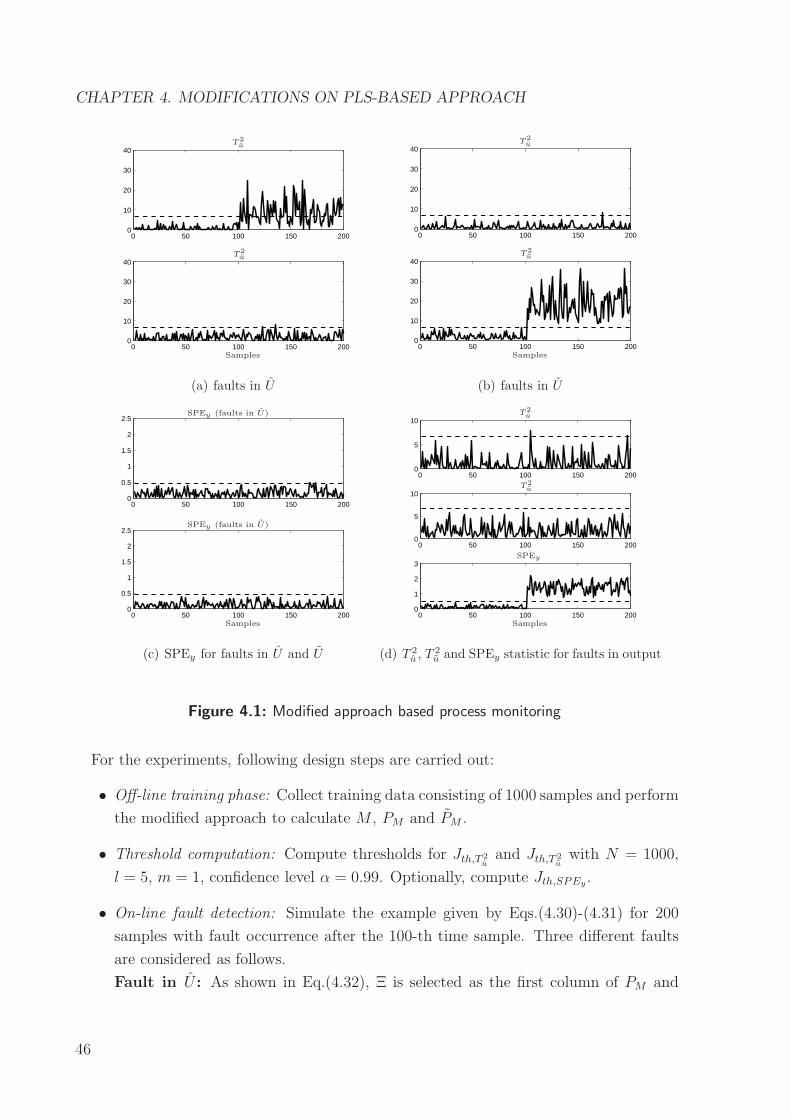
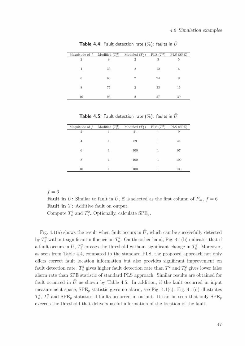
4.6 Simulation examples . . . . . . . . . . . . . . . . . . . . . . . . . . . . . . 45


5 Subspace aided data-driven approach 49

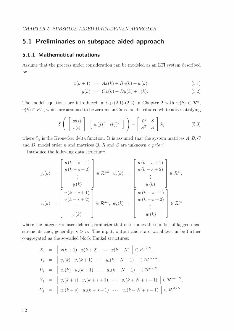
5.1 Preliminaries on subspace aided approach . . . . . . . . . . . . . . . . . . 52

5.1.1 Mathematical notations . . . . . . . . . . . . . . . . . . . . . . . . 52

5.1.2 Relations between SIM and PCA . . . . . . . . . . . . . . . . . . . 54

5.1.3 Identification of parity space . . . . . . . . . . . . . . . . . . . . . . 55

5.2 Residual generator design . . . . . . . . . . . . . . . . . . . . . . . . . . . 56

5.2.1 Single residual generation . . . . . . . . . . . . . . . . . . . . . . . 56

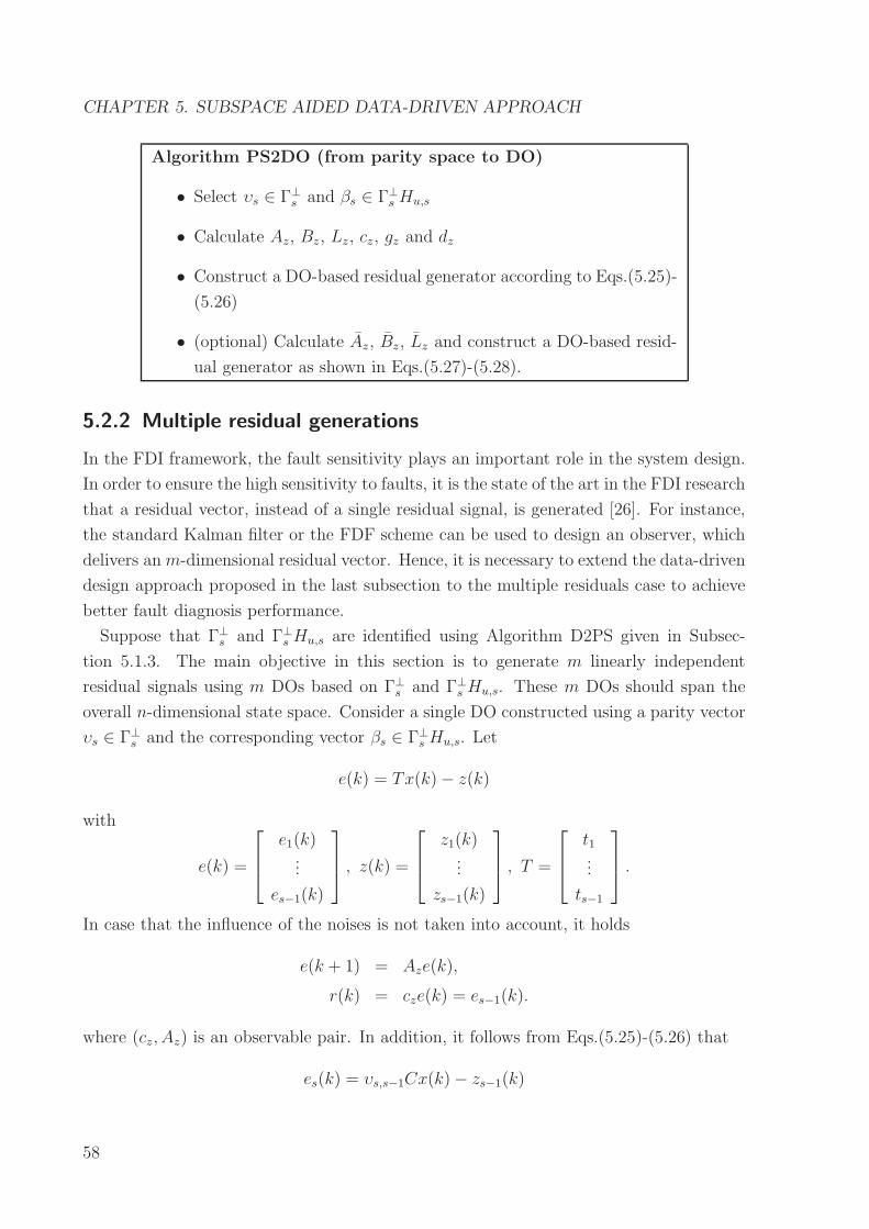
5.2.2 Multiple residual generations . . . . . . . . . . . . . . . . . . . . . . 58

5.2.3 A PCA-like approach . . . . . . . . . . . . . . . . . . . . . . . . . . 62

5.3 State Estimator design . . . . . . . . . . . . . . . . . . . . . . . . . . . . . 64


6 On recursive and adaptive design issues 68


6.2 Subspace tracking technique . . . . . . . . . . . . . . . . . . . . . . . . . . 69

6.2.1 FOP-based subspace tracking . . . . . . . . . . . . . . . . . . . . . 69

6.2.2 DPM-based subspace tracking . . . . . . . . . . . . . . . . . . . . . 71

6.2.3 Recursive updating algorithm . . . . . . . . . . . . . . . . . . . . . 72

VI

Contents

6.3 Adaptive DO-based residual generator . . . . . . . . . . . . . . . . . . . . 72

6.3.1 Mathematical notations . . . . . . . . . . . . . . . . . . . . . . . . 73

6.3.2 The adaptive residual generator scheme . . . . . . . . . . . . . . . . 73

6.3.3 Stability and exponential convergence . . . . . . . . . . . . . . . . . 75

6.4 Simulation examples . . . . . . . . . . . . . . . . . . . . . . . . . . . . . . 78


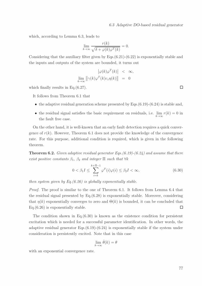
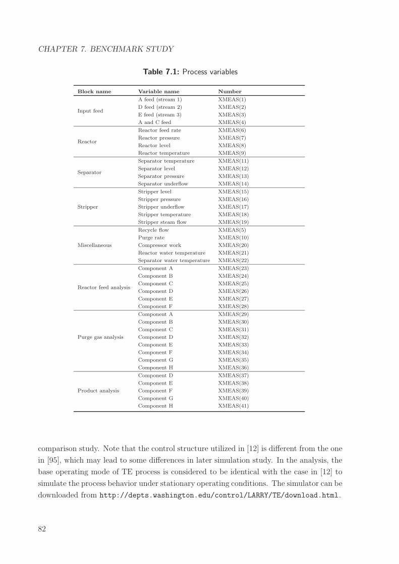
7 Benchmark study 80

7.1 Benchmark description . . . . . . . . . . . . . . . . . . . . . . . . . . . . . 80

7.1.1 TE process . . . . . . . . . . . . . . . . . . . . . . . . . . . . . . . 80

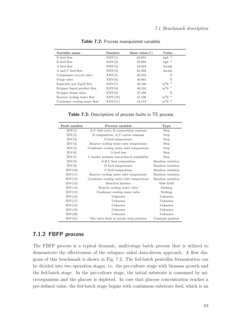
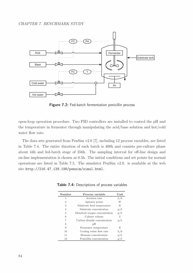
7.1.2 FBFP process . . . . . . . . . . . . . . . . . . . . . . . . . . . . . . 83

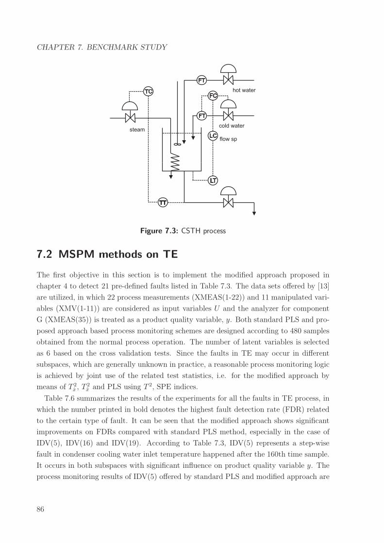
7.1.3 CSTH process . . . . . . . . . . . . . . . . . . . . . . . . . . . . . . 85

7.2 MSPM methods on TE . . . . . . . . . . . . . . . . . . . . . . . . . . . . . 86

7.3 Subspace approach on FBFP . . . . . . . . . . . . . . . . . . . . . . . . . . 91

7.4 Adaptive approach on CSTH . . . . . . . . . . . . . . . . . . . . . . . . . . 93


8 Conclusions and future work 96

Bibliography 98

VII

Notation and symbols

Abbreviations

FD Fault detection

FDI Fault detection and isolation

FDIA Fault detection, isolation, and analysis

LTI Linear time invariant

FDF Fault detection filter

DO Diagnostic observer

MSPM Multivariate statistical process monitoring

SIM Subspace identification method

PCA Principal component analysis

PCs Principal components

PLS Partial least squares

LVs Latent variables

FDA Fisher discriminant analysis

ICA Independent component analysis

ICs Independent components

SVD Singular value decomposition

GLR Generalized likelihood ratio

TPLS Total projection to latent structure

DPM Data projection method

FOP First-order perturbation theory

TE Tennessee Eastman

FBFP Fed-batch fermentation penicillin

CSTH Continuous stirred tank heater

Mathematical symbols

‖ ‖ 2-norm

a Estimate of a

VIII

NOTATION AND SYMBOLS

a Estimate error of a

AT Transpose of A

A⊥ Orthogonal complement of A

A† Pseudo inverse of A

∈ belongs to

R Set of real numbers

Rm Set of m-dimensional real vectors

Rl×m Set of l ×m dimensional real matrices

Im×m m×m identity matrix

Control theoretical symbols

n System order

k Discrete time sample

A System matrix

B Input matrix

C Output matrix

D Feed-though matrix

Ed Disturbance matrix

Fd Disturbance feed-through matrix

Ef Process fault distribution matrix

Ff Sensor fault distribution matrix

l Number of inputs

m Number of outputs

u Input signal vector

y Output signal vector

x State variable vector

w Process noise vector

v Sensor noise vector

d Unknown disturbance vector

f Fault signal vector

r Residual signal vector

Γs Extended observability matrix

Γ⊥s Left null complement

Hu,s Input distribution matrix

Yf Future output Hankel matrix

Uf Future input Hankel matrix

IX

NOTATION AND SYMBOLS

Yp Past output Hankel matrix

Up Past input Hankel matrix

N Length of sample size

s Order of parity vector

υs Parity vector corresponding to output

βs Parity vector corresponding to input

Lz Observer gain matrix

Z Process variable matrix

U Input matrix

Y Output matrix

β Number of principal components

γ Number of latent variables

Jth Threshold value for fault detection

Statistical symbols

Φ Sample covariance matrix

χ2 Chi-square distribution

F F distribution

U Uniform distribution

N Gaussian distribution

E Mathematical Expectation

α Confidence level

T 2 T-square statistic

SPE Squared prediction error

X

Abstract

Due to the increasing demands on system performance, production quality as well as eco-

nomic operation, modern technical systems become more complicated and the automation

degrees are significantly growing. To ensure the safety and reliability of such complicated

processes, an effective fault diagnosis system is of prime importance in process industry

nowadays. Although the model-based fault diagnosis theory has been well established,

it is still difficult to establish mathematical model by means of the first principles for

large-scale process.

On the other hand, a large amount of historical data from regular sensor measurements,

event-logs and records are often available in such industrial processes. Motivated by this

observation, it is of great interest to design fault diagnosis schemes only based on the

available process data. Hence, development of efficient data-driven fault diagnosis schemes

for different operating conditions is the primary objective of this thesis.

This thesis is firstly dedicated to the modifications on the standard multivariate statis-

tical process monitoring approaches. The modified approaches are considerably simple,

and most importantly, avoid the drawbacks of the standard techniques. As a result, the

proposed approaches are able to provide enhanced fault diagnosis performance on the

applications under stationary operating conditions.

The further study of this thesis focuses on developing reliable fault diagnosis schemes for

dynamic processes under industrial operating conditions. Instead of identifying the entire

process model, primary fault diagnosis can be efficiently realized by the identification of

key components. Advanced design schemes like multiple residuals generator and state

observer are also investigated to ensure high fault sensitivity performance.

For the large-scale processes involving changes, e.g. in operating regimes or in the

manipulated variables, the recursive and adaptive techniques are studied to cope with

such uncertainty issues. A novel data-driven adaptive scheme is proposed, whose stability

and convergence rate are analytically proven. Compared to the standard techniques,

this approach does not involve complicated on-line computation and produces consistent

estimate of the unknown parameters.

To illustrate the effectiveness of the derived data-driven approaches, three industrial

benchmark processes, i.e. the Tennessee Eastman chemical plant, the fed-batch fermen-

XI

ABSTRACT

tation penicillin process and the continuously stirred tank heater, are finally considered

in this thesis.

XII

1 Introduction

Due to the increasing demands on system performance, production quality as well as

economic operation, modern technical processes become more complicated and the au-

tomation degrees of such systems are significantly growing. The safety and reliability

issues on the complicated processes receive more attention and become the most critical

factors in process design nowadays. On the other hand, the complete reliance on human

operators to deal with abnormal events has become increasingly difficult as shown by the

following facts:

• It is claimed that about 70% of the industrial accidents are caused by human errors

[106].

• Only the petrochemical industry in the US incurs approximately 20 billion dollars

in annual losses due to process abnormalities [85]. Similar accidents cost the British

27 billion dollars in economic loss every year [68].

• The consequences of the accidents are not only performance degradation, economic

loss but also more serious catastrophes such as the Three Mile Island and Chernobyl

in nuclear industry.

Based on these observations, the integration of an automated fault diagnosis scheme is

essential to ensure a reliable abnormal event management, which not only informs about

process abnormalities in time but also makes further suitable actions to remove the unde-

sirable influence from the process. Depending on the different operational constraints and

requirements of the underlying applications, design of superior and robust fault diagnosis

scheme has been an active research field in the control community during the past several

decades. This chapter attempts to summarize some of the major developments in this

field. The motivations and objectives of the thesis are also presented.

1.1 Basic concepts on fault diagnosis

Faults in process equipments, instructions or within the process can lead to an unper-

mitted deviation from the normal behavior of the plant and thus degrade overall system

1

CHAPTER 1. INTRODUCTION

performance. For instance, in an industrial chemical process, the faults are likely to occur

in sensors (e.g. analyzer contamination, biased measurements), actuators (e.g., valves,

pumps and pipes) and process itself (e.g. catalyst poisoning, heat exchanger fouling).

A single fault can harm not only the functional components, but also the whole plant

through the coupled control loops and feedback systems. To deal with such problems, a

fault diagnosis system is desired to monitor the operating condition of the whole plant

and achieve prompt detection and diagnosis of process malfunctions automatically. As

pointed out in [21], the overall concept of fault diagnosis consists of the following three

essential tasks:

Fault detection: detection of the occurrence of faults in the functional units of the pro-

cess, which lead to the undesired or intolerable behavior of the whole system

Fault isolation: localization (classification) of different faults

Fault analysis or identification: determination of the type, magnitude and cause of the

fault.

According to different performance requirements, a fault diagnosis system is called fault

detection (FD) system, fault detection and isolation (FDI) system or fault detection,

isolation, and analysis (FDIA) system.

In technical terms, the so-called redundancy plays a central role for a successful fault

diagnosis [21]. The so-called hardware redundancy is one of the traditional ways to

create system redundancy, in which the crucial components are reconstructed using the

identical hardware. A fault can be directly detected and localized by the deviation between

the output of actual hardware component and the one of its redundancy. Although

an extremely reliable fault detection and isolation can be achieved, the application of

hardware redundancy is only restricted to the case of a number of key components due

to their higher cost involved in reconstruction. Associated with the concept of hardware

redundancy, the so-called software redundancy or analytical redundancy is more

efficient, whose basic idea is to replace the expensive hardware components by a model

implemented in the software form in order to reconstruct the process behavior on-line.

The fault detection is achieved by checking the so-called residual, which represents the

difference between the measured process variables, e.g. output signals y, and their software

redundancy y, i.e.

residual = y − y.

The basic model-based fault diagnosis scheme including residual generation and

residual evaluation is represented by Fig. 1.1. In general, the model can be quantita-

2

1.1 Basic concepts on fault diagnosis

Process

Model-

Inputs Outputs

Residual Residualprocessing

Decisionlogic

Residual generation Residual evaluation

Model-based fault diagnosis system

Knowledgeof faults

Figure 1.1: Basic model-based fault diagnosis scheme

tive (based on the first principles), qualitative (based on the if-then-else rules, decision

trees etc.) or process history data based [106], [107], [108]:

Quantitative model-based approach: Most of the works on quantitative model-based

approach are based on general input-output or state space model, which is usually

developed based on the physics and mathematics knowledge of the process. From

the 70s, observers and Kalman filtering theories have been widely used for residual

generation in dynamic systems [2], [38], [39] [118]. The so-called parity relation has

been firstly introduced in [117], whose basic idea is to check the parity relation of the

model with available process input and output measurements. Further developments

of this approach can be found in [17], [42], [43]. In addition, the so-called parameter

estimation approach has been proposed to detect the unmeasurable parameter drift

[52].

Based on these approaches, a large number of advanced fault diagnosis methods

were developed to handle the issues of disturbances, model uncertainties, robust,

optimization designs, etc. Nowadays, the quantitative model-based fault diagnosis

techniques have been established into a well-founded theoretical framework and

successfully demonstrated by a great number of applications in industrial processes

and automatic control systems, see [8], [11], [21], [40], [53], [88], [98]. Reviews

and analysis of current development of the quantitative model-based fault diagnosis

techniques can be found in [27], [50], [106], [112], [115], [131].

Qualitative model-based approach: Unlike quantitative model, in which the relation-

ships between inputs and outputs of the process are described in terms of mathe-

matical functions, the relationships in qualitative model are expressed by qualitative

functions centered around different units of the process. Based on such a qualitative

3


model, any fault diagnostic strategy requires a knowledge base, which contains a

large set of if-then-else rules that mimics the cognitive behavior of a human ex-

pert. In addition, an efficient search mechanism shall also be included to make final

decision from given facts. The qualitative models are suitable to be utilized on large-

scale processes which are difficult to be modeled based on the first principals. On

the other hand, since the knowledge base does not have a fundamental understand-

ing of the physics of underlying process, it is difficult to update or accommodate in

case that new conditions are encountered. More detailed discussion on qualitative

approach can be found in [107] and the references therein.

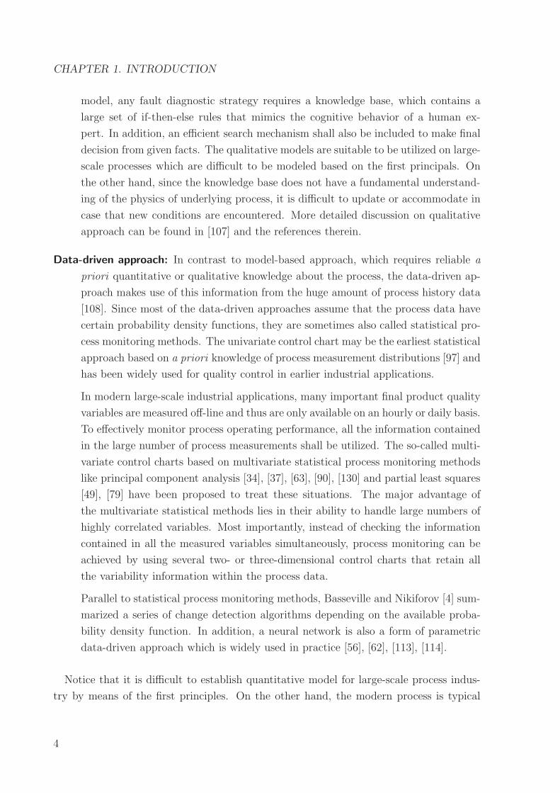
Data-driven approach: In contrast to model-based approach, which requires reliable a

priori quantitative or qualitative knowledge about the process, the data-driven ap-

proach makes use of this information from the huge amount of process history data

[108]. Since most of the data-driven approaches assume that the process data have

certain probability density functions, they are sometimes also called statistical pro-

cess monitoring methods. The univariate control chart may be the earliest statistical

approach based on a priori knowledge of process measurement distributions [97] and

has been widely used for quality control in earlier industrial applications.

In modern large-scale industrial applications, many important final product quality

variables are measured off-line and thus are only available on an hourly or daily basis.

To effectively monitor process operating performance, all the information contained

in the large number of process measurements shall be utilized. The so-called multi-

variate control charts based on multivariate statistical process monitoring methods

like principal component analysis [34], [37], [63], [90], [130] and partial least squares

[49], [79] have been proposed to treat these situations. The major advantage of

the multivariate statistical methods lies in their ability to handle large numbers of

highly correlated variables. Most importantly, instead of checking the information

contained in all the measured variables simultaneously, process monitoring can be

achieved by using several two- or three-dimensional control charts that retain all

the variability information within the process data.

Parallel to statistical process monitoring methods, Basseville and Nikiforov [4] sum-

marized a series of change detection algorithms depending on the available proba-

bility density function. In addition, a neural network is also a form of parametric

data-driven approach which is widely used in practice [56], [62], [113], [114].

Notice that it is difficult to establish quantitative model for large-scale process indus-

try by means of the first principles. On the other hand, the modern process is typical

4

1.2 Motivation and objective

dynamic process with different operating regimes, which can not be directly treated by

the basic statistical approaches. Therefore, the extension and combination of the advan-

tages of model-based and data-driven techniques have nowadays gained more attention

to accommodate large-scale and complex process. A straightforward way to achieve this

purpose is to utilize the process history data for model identification and based on it,

the well-established model-based techniques can be used to design efficient fault diagnosis

system.

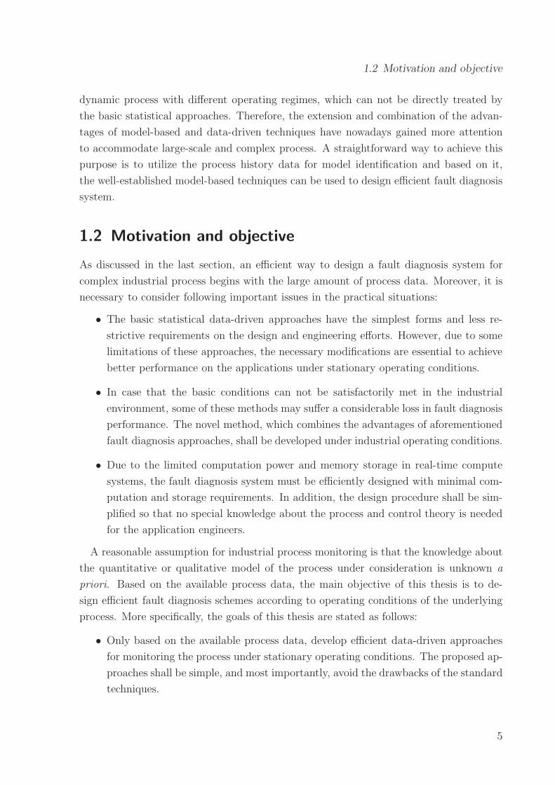
1.2 Motivation and objective

As discussed in the last section, an efficient way to design a fault diagnosis system for

complex industrial process begins with the large amount of process data. Moreover, it is

necessary to consider following important issues in the practical situations:

• The basic statistical data-driven approaches have the simplest forms and less re-

strictive requirements on the design and engineering efforts. However, due to some

limitations of these approaches, the necessary modifications are essential to achieve

better performance on the applications under stationary operating conditions.

• In case that the basic conditions can not be satisfactorily met in the industrial

environment, some of these methods may suffer a considerable loss in fault diagnosis

performance. The novel method, which combines the advantages of aforementioned

fault diagnosis approaches, shall be developed under industrial operating conditions.

• Due to the limited computation power and memory storage in real-time compute

systems, the fault diagnosis system must be efficiently designed with minimal com-

putation and storage requirements. In addition, the design procedure shall be sim-

plified so that no special knowledge about the process and control theory is needed

for the application engineers.

A reasonable assumption for industrial process monitoring is that the knowledge about

the quantitative or qualitative model of the process under consideration is unknown a

priori. Based on the available process data, the main objective of this thesis is to de-

sign efficient fault diagnosis schemes according to operating conditions of the underlying

process. More specifically, the goals of this thesis are stated as follows:

• Only based on the available process data, develop efficient data-driven approaches

for monitoring the process under stationary operating conditions. The proposed ap-

proaches shall be simple, and most importantly, avoid the drawbacks of the standard

techniques.

5


• On the applications under industrial operating conditions, develop reliable fault

diagnosis scheme for dynamic processes. Instead of identifying the entire process

model, primary fault diagnosis shall be realized with the identification of key com-

ponents. It is also desirable to investigate the advanced design schemes in order to

ensure high fault sensitivity performance.

• In practice, since the process parameters are likely to vary around their nominal

values, the fault diagnosis system must have scope for possible adaptation. The

adaptive design scheme shall consider on-line storage and computation constraints,

and most importantly, possess desired performance on stability and convergence

rate.

• The developed data-driven fault diagnosis approaches must be demonstrated on

industrial benchmark plants, which should be good approximations of complex in-

dustrial processes under different operating conditions.

The data sets used for fault diagnosis system design can be obtained from either avail-

able process logs or experimental tests. In case that a process simulator is available, the

data generated from such simulations are also useful. In this thesis, three well-known

industrial benchmark processes are utilized to evaluate the effectiveness of the proposed

approaches for fault diagnosis purpose.

1.3 Outline of the thesis

This thesis is organized as follows. Chapter 2 includes preliminaries of fault diagnosis tech-

niques with technical systems notations, which serve as fundamental basis in forthcoming

chapters. The basic model-based approaches like parity space and diagnostic observer are

firstly introduced in this chapter. The subspace identification method is also discussed

therein. The most popular multivariate statistical process monitoring approaches like

principal component analysis and partial least squares, are finally reviewed. Based on it,

the modifications of these basic statistical approaches are introduced in Chapter 3 and 4.

In Chapter 3, the modifications on principal component analysis based fault diagnosis

technique are discussed. A new test statistic is firstly proposed, which delivers an optimal

fault detection performance and is considerably less complicated than the standard one.

The further study is dedicated to the analysis of fault sensitivity. The fault identification

issue is finally discussed in the proposed framework.

Chapter 4 begins with the partial least squares based fault diagnosis technique. A new

approach is proposed to overcome the drawbacks of the standard approach. The associated

6

1.3 Outline of the thesis

computation cost for the proposed approach is considerably lower, and most importantly,

the novel approach provides a clear interpretation of the correlation model. Based on this

approach, a fault detection scheme is then developed, in which only two test statistics

are used for monitoring input measurement space that offers further efficiency compared

to the existing methods. An algorithm for fault identification is finally presented in this

chapter.

In Chapter 5, a subspace aided data-driven approach is presented to achieve fault detec-

tion in dynamic processes under industrial operating conditions. The study is dedicated

to extending the single residual generation scheme to multiple case in order to ensure

the high sensitivity to the faults. The proposed multiple diagnostic observers can also be

utilized to construct state observer for the process monitoring and control purposes.

Chapter 6 mainly discusses the uncertainty issue in industrial applications. Two recur-

sive algorithms for subspace tracking are firstly proposed. Both algorithms avoid repeated

calculations of standard singular value decomposition and provide approximate result in

an efficient way. The further study is dedicated to developing a data-driven adaptive di-

agnostic observer based residual generation scheme, whose stability and convergence rate

can be analytically proven.

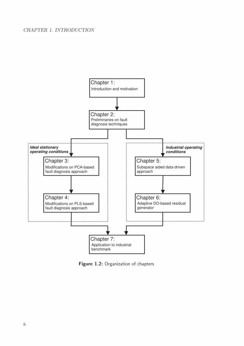
Chapter 7 illustrates the applications of the algorithms developed in Chapters 3-6.

For this task, three well-known industrial benchmark processes, i.e. Tennessee Eastman

process, fed batch fermentation penicillin process and continuously stirred tank heater,

are considered to simulate their behaviors under different operating conditions. The

experiments are carried out under scenarios involving different types of faults existing in

the industrial processes. For simplicity in reading, the organization of chapters is also

shown in Fig. 1.2 on the following page. This thesis ends with the conclusions and the

discussion on future work.

7


Chapter 1:

Chapter 2:

Chapter 3: Chapter 5:

Chapter 4: Chapter 6:

Chapter 7:

Introduction and motivation

Preliminaries on faultdiagnosis techniques

Modifications on PCA-basedfault diagnosis approach

Modifications on PLS-basedfault diagnosis approach

Subspace aided data-drivenapproach

Adaptive DO-based residualgenerator

Application to industrialbenchmark

Ideal stationaryoperating conditions

Industrial operatingconditions

Figure 1.2: Organization of chapters

8

2 Fault diagnosis techniques

As discussed in Chapter 1, the basic idea of fault diagnosis is to generate the output

redundancy through a “model” which is able to offer precise behavior of process under

consideration. Any significant deviation between the actual measurement and the redun-

dancy generated by process model should sufficiently indicate the existence of abnormal

situation. Due to the high cost to achieve hardware redundancy, the most efficient way

for a successful fault diagnosis is to create the redundancy analytically.

During the last two decades, the model-based fault diagnosis schemes are intensively

studied. Since the majority of these approaches involve rigorous development of process

models based on the first principles, later identification technique that extracts transfer

function [77] or state space model becomes a necessary step prior to the design. For this

purpose, subspace identification methods that identify the complete state space matrices

have been successfully implemented [36], [91], [105].

Parallel to the aforementioned techniques, the data-driven approaches, which extract

necessary information through large amount of process data, are currently receiving con-

siderably increasing attention both in application and in research domains. Thanks to

their simple forms and less requirements on the design and engineering efforts, the data-

driven methods become more popular in many industry sectors, especially for large-scale

industrial applications [96].

The objective of this chapter is to summarize the preliminaries of the fault diagnosis

techniques, which serve as the fundamentals of this thesis.

2.1 Description of technical systems

According to the process dynamics and modeling aims, technical processes can be de-

scribed by different system model types, among which the linear time invariant (LTI)

system is the mostly used one and assumed as a good starting point for modeling and

design phase. The standard form of the state space representation of a discrete time LTI

9

CHAPTER 2. FAULT DIAGNOSIS TECHNIQUES

system is given by

x(k + 1) = Ax(k) +Bu(k), x(0) = x0, (2.1)

y(k) = Cx(k) +Du(k) (2.2)

where x ∈ Rn is the state vector, x0 is the initial condition of the system, u ∈ Rl is the

input vector and y ∈ Rm is the output vector. System matrices A,B,C and D are real

constant matrices with appropriate dimensions. Considering that the subsequent study

mainly focuses on data-driven design of fault diagnosis systems based on sampled process

measurements, the state space model is defined only in the discrete time LTI framework.

In order to describe the deterministic disturbances, an additional input vector d ∈ Rkd

is integrated into Eqs.(2.1)-(2.2) as follows:

x(k + 1) = Ax(k) +Bu(k) + Edd(k), (2.3)

y(k) = Cx(k) +Du(k) + Fdd(k) (2.4)

where Ed and Fd are disturbance distribution matrices of compatible dimensions. If the

process is corrupted by stochastic noises, e.g. process and measurement noises, the state

space representation becomes

x(k + 1) = Ax(k) +Bu(k) + w(k), (2.5)

y(k) = Cx(k) +Du(k) + v(k) (2.6)

where the stochastic disturbance signals w ∈ Rn, v ∈ Rm are often white noise sequences

with known mean and covariance matrix.

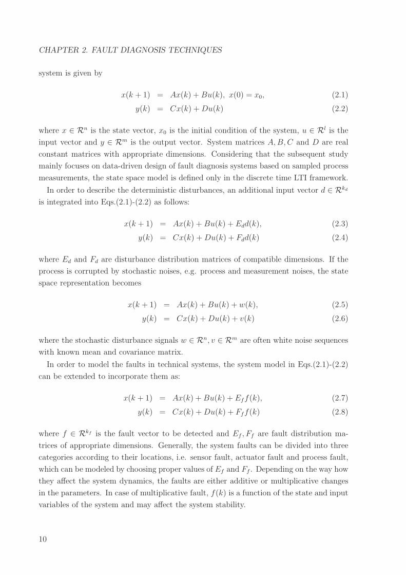
In order to model the faults in technical systems, the system model in Eqs.(2.1)-(2.2)

can be extended to incorporate them as:

x(k + 1) = Ax(k) +Bu(k) + Eff(k), (2.7)

y(k) = Cx(k) +Du(k) + Fff(k) (2.8)

where f ∈ Rkf is the fault vector to be detected and Ef , Ff are fault distribution ma-

trices of appropriate dimensions. Generally, the system faults can be divided into three

categories according to their locations, i.e. sensor fault, actuator fault and process fault,

which can be modeled by choosing proper values of Ef and Ff . Depending on the way how

they affect the system dynamics, the faults are either additive or multiplicative changes

in the parameters. In case of multiplicative fault, f(k) is a function of the state and input

variables of the system and may affect the system stability.

10

2.2 Model-based fault diagnosis techniques


Model-based techniques have been remarkably developed since 80’s and their efficiency

for detecting faults has been demonstrated by a great number of applications in indus-

trial processes and automatic control systems. Among the existing model-based fault

diagnosis schemes, the so-called observer-based and parity relation based methods, which

are developed in the framework of well-established modern control theory, have received

much attention during last two decades. Brief introductions of the related topics will be

included in this section.

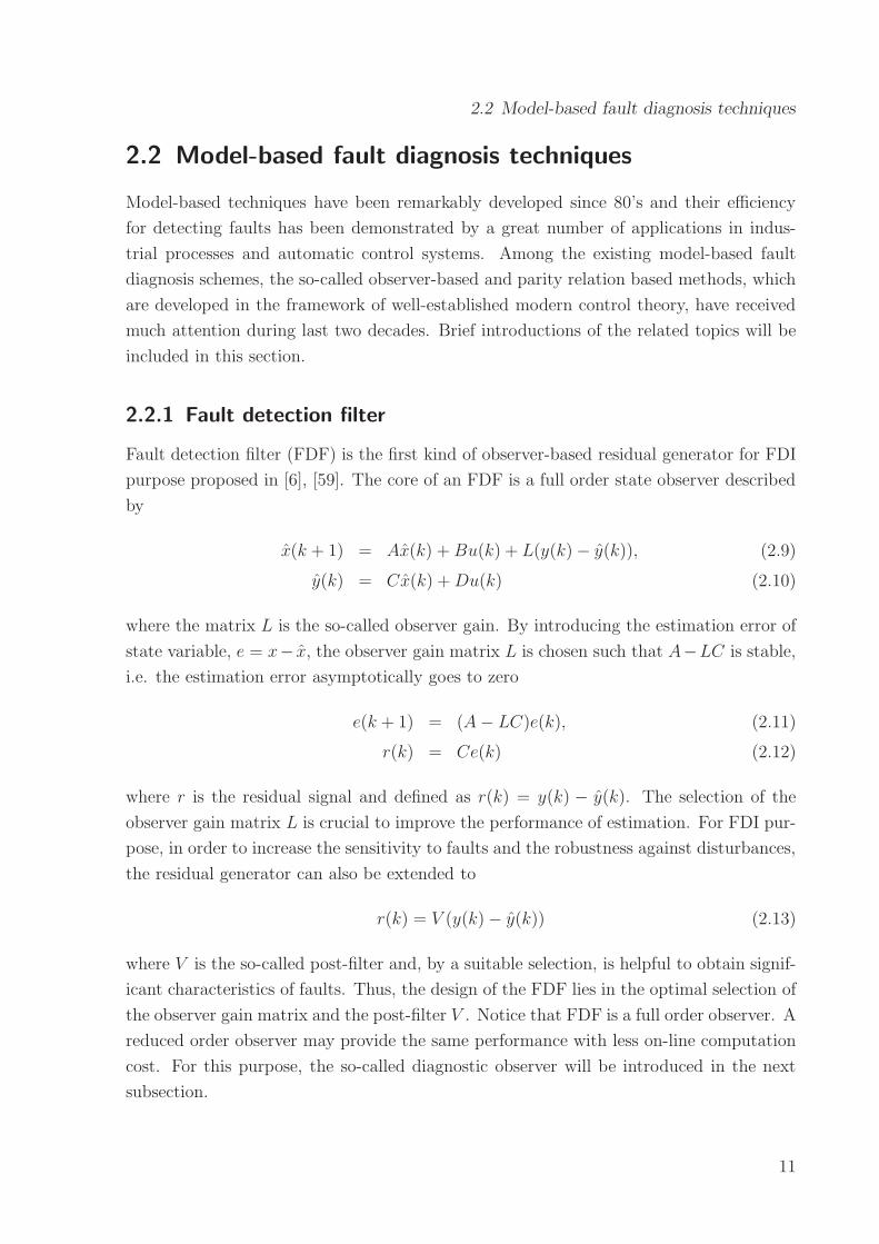
2.2.1 Fault detection filter

Fault detection filter (FDF) is the first kind of observer-based residual generator for FDI

purpose proposed in [6], [59]. The core of an FDF is a full order state observer described

by

x(k + 1) = Ax(k) +Bu(k) + L(y(k)− y(k)), (2.9)

y(k) = Cx(k) +Du(k) (2.10)

where the matrix L is the so-called observer gain. By introducing the estimation error of

state variable, e = x− x, the observer gain matrix L is chosen such that A−LC is stable,

i.e. the estimation error asymptotically goes to zero

e(k + 1) = (A− LC)e(k), (2.11)

r(k) = Ce(k) (2.12)

where r is the residual signal and defined as r(k) = y(k) − y(k). The selection of the

observer gain matrix L is crucial to improve the performance of estimation. For FDI pur-

pose, in order to increase the sensitivity to faults and the robustness against disturbances,

the residual generator can also be extended to

r(k) = V (y(k)− y(k)) (2.13)

where V is the so-called post-filter and, by a suitable selection, is helpful to obtain signif-

icant characteristics of faults. Thus, the design of the FDF lies in the optimal selection of

the observer gain matrix and the post-filter V . Notice that FDF is a full order observer. A

reduced order observer may provide the same performance with less on-line computation

cost. For this purpose, the so-called diagnostic observer will be introduced in the next

subsection.

11


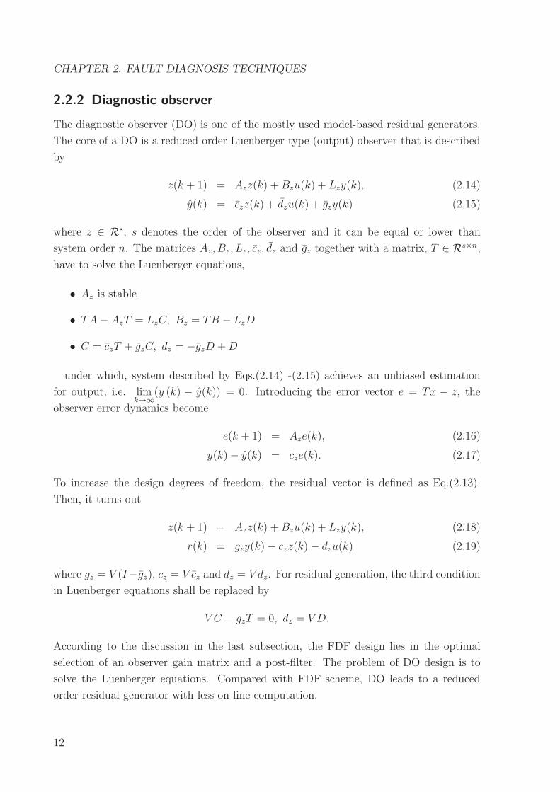
2.2.2 Diagnostic observer

The diagnostic observer (DO) is one of the mostly used model-based residual generators.

The core of a DO is a reduced order Luenberger type (output) observer that is described

by

z(k + 1) = Azz(k) +Bzu(k) + Lzy(k), (2.14)

y(k) = czz(k) + dzu(k) + gzy(k) (2.15)

where z ∈ Rs, s denotes the order of the observer and it can be equal or lower than

system order n. The matrices Az, Bz, Lz, cz, dz and gz together with a matrix, T ∈ Rs×n,

have to solve the Luenberger equations,

• Az is stable

• TA− AzT = LzC, Bz = TB − LzD

• C = czT + gzC, dz = −gzD +D

under which, system described by Eqs.(2.14) -(2.15) achieves an unbiased estimation

for output, i.e. limk→∞

(y (k) − y(k)) = 0. Introducing the error vector e = Tx − z, the

observer error dynamics become

e(k + 1) = Aze(k), (2.16)

y(k)− y(k) = cze(k). (2.17)

To increase the design degrees of freedom, the residual vector is defined as Eq.(2.13).

Then, it turns out

z(k + 1) = Azz(k) +Bzu(k) + Lzy(k), (2.18)

r(k) = gzy(k)− czz(k)− dzu(k) (2.19)

where gz = V (I−gz), cz = V cz and dz = V dz. For residual generation, the third condition

in Luenberger equations shall be replaced by

V C − gzT = 0, dz = V D.

According to the discussion in the last subsection, the FDF design lies in the optimal

selection of an observer gain matrix and a post-filter. The problem of DO design is to

solve the Luenberger equations. Compared with FDF scheme, DO leads to a reduced

order residual generator with less on-line computation.

12


2.2.3 Parity space approach

Parallel to the observer-based residual generation approaches, the so-called parity space

approach has been proposed by Chow and Willsky [17] in the early 80’s and serves as one

of the simplest ways for FDI. Based on the state space model, the parity relation, instead

of an observer, is used for residual generation. Suppose that the system described by

Eqs.(2.1)-(2.2) is observable and rank(C) = m. The system can be recursively expressed

as follows:

y(k − s+ 1) = Cx(k − s+ 1) +Du(k − s+ 1),

y(k − s+ 2) = Cx(k − s+ 2) +Du(k − s+ 2)

= CAx(k − s+ 1) + CBu(k − s+ 1) +Du(k − s+ 2),

and so on. Repeating this procedure yields:

y(k) = CAs−1x(k − s+ 1) + CAs−2Bu(k − s+ 1) + · · ·+ CBu(k − 1) +Du(k). (2.20)

Introducing the following notations for input and output data

ys(k) =

y (k − s+ 1)

y (k − s+ 2)...

y (k)

∈ Rsm, us(k) =

u (k − s+ 1)

u (k − s+ 2)...

u (k)

∈ Rsl,

the system can be rewritten into the following compact form

ys(k) = Γsx(k − s+ 1) +Hu,sus(k) (2.21)

where

Γs =

C

CA...

CAs−1

∈ Rsm×n, Hu,s =

D 0 · · · 0

CB D · · · 0...

.... . .

...

CAs−2B · · · CB D

.

Eq.(2.21) is the so-called parity relation, which describes the input and output relationship

with the past state variable x(k − s+ 1).

Assume that (C,A) is observable, for s > n, the following rank condition holds:

rank (Γs) = n (2.22)

which ensures that there exists at least a row vector vs( 6= 0) ∈ R1×sm such that

vsΓs = 0. (2.23)

13


The vectors satisfying Eq.(2.23) are termed as parity vectors, whose set

Ps = {vs|vsΓs = 0} (2.24)

is called the parity space of the s-th order.

Consequently, a parity relation based residual generator can be constructed as

r(k) = vs(ys(k)−Hu,sus(k)). (2.25)

In case that the system is corrupted by faults and disturbances, it follows that

ys(k) = Γsx(k − s+ 1) +Hu,sus(k) +Hf,sfs(k) +Hd,sds(k) (2.26)

where

fs(k) =

f (k − s+ 1)

f (k − s+ 2)...

f (k)

, Hf,s =

Ff O · · · O

CEf Ff. . .

......

. . .. . . O

CAs−2Ef CAs−3Ef · · · Ff

,

ds(k) =

d (k − s+ 1)

d (k − s+ 2)...

d (k)

, Hd,s =

Fd O · · · O

CEd Fd. . .

......

. . .. . . O

CAs−2Ed CAs−3Ed · · · Fd

.

Thus, residual signal presented in Eq.(2.25) becomes

r(k) = vs (Hd,sds(k) +Hf,sfs(k)) . (2.27)

The design of parity relation based residual generator can be achieved in a straightforward

manner. The only parameter to be designed is the parity vector. On the other hand, the

implementation form of Eq.(2.25), which not only includes the temporal but also the

past input and output data, is not ideal for on-line realization. Based on the research on

the characterization of parity space and Luenberger equations, Ding et al. [22] revealed

interesting interconnections between DO and parity space.

2.2.4 Interconnections between DO and parity space

Although the implementation forms of DO and parity space based residual generators are

different, the one-to-one mapping between these two approaches has been proposed by

Ding et al. [22], which reveals that all design approaches based on parity space can be

14

2.3 Subspace identification method

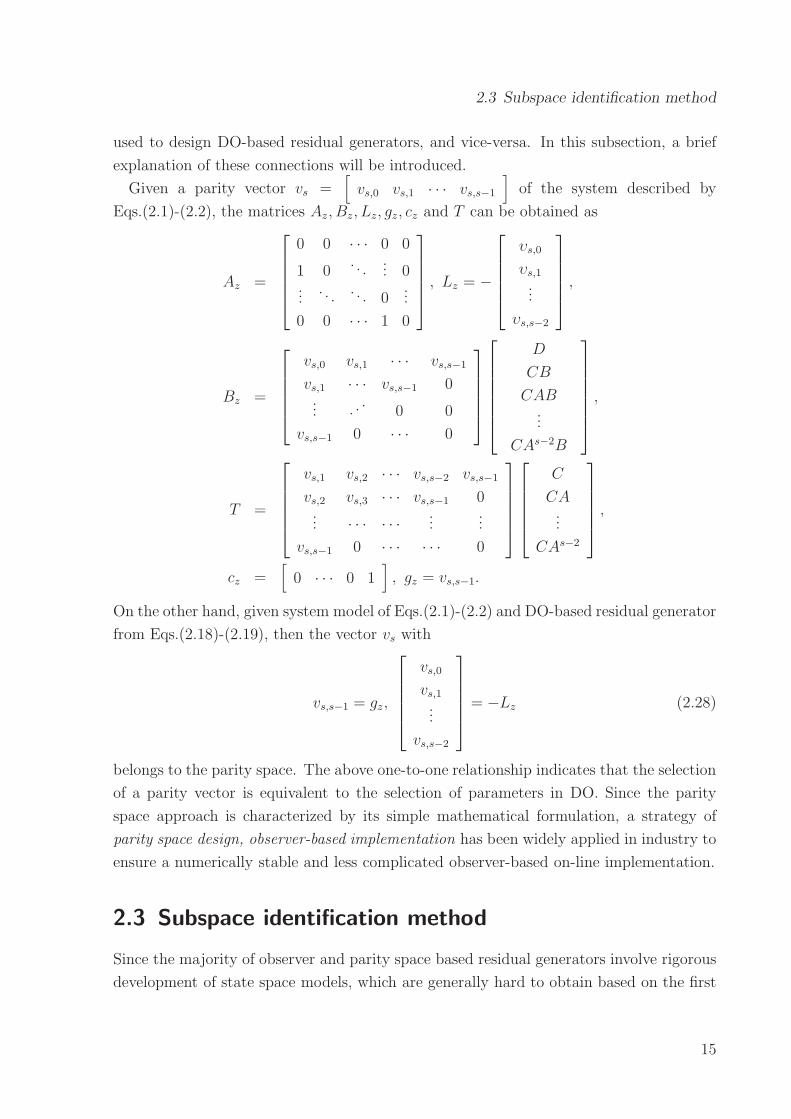
used to design DO-based residual generators, and vice-versa. In this subsection, a brief

explanation of these connections will be introduced.

Given a parity vector vs =[

vs,0 vs,1 · · · vs,s−1

]

of the system described by

Eqs.(2.1)-(2.2), the matrices Az, Bz, Lz, gz, cz and T can be obtained as

Az =

0 0 · · · 0 0

1 0. . .

... 0...

. . .. . . 0

...

0 0 · · · 1 0

, Lz = −

υs,0

υs,1...

υs,s−2

,

Bz =

vs,0 vs,1 · · · vs,s−1

vs,1 · · · vs,s−1 0... . .

.0 0

vs,s−1 0 · · · 0

D

CB

CAB...

CAs−2B

,

T =

vs,1 vs,2 · · · vs,s−2 vs,s−1

vs,2 vs,3 · · · vs,s−1 0... · · · · · ·

......

vs,s−1 0 · · · · · · 0

C

CA...

CAs−2

,

cz =[

0 · · · 0 1]

, gz = vs,s−1.

On the other hand, given system model of Eqs.(2.1)-(2.2) and DO-based residual generator

from Eqs.(2.18)-(2.19), then the vector vs with

vs,s−1 = gz,

vs,0

vs,1...

vs,s−2

= −Lz (2.28)

belongs to the parity space. The above one-to-one relationship indicates that the selection

of a parity vector is equivalent to the selection of parameters in DO. Since the parity

space approach is characterized by its simple mathematical formulation, a strategy of

parity space design, observer-based implementation has been widely applied in industry to

ensure a numerically stable and less complicated observer-based on-line implementation.

2.3 Subspace identification method

Since the majority of observer and parity space based residual generators involve rigorous

development of state space models, which are generally hard to obtain based on the first

15


Processdata

Modelidentification

Fault diagnosissystem design

On-lineimplementation

Processmodel

System identification Fault diagnosis

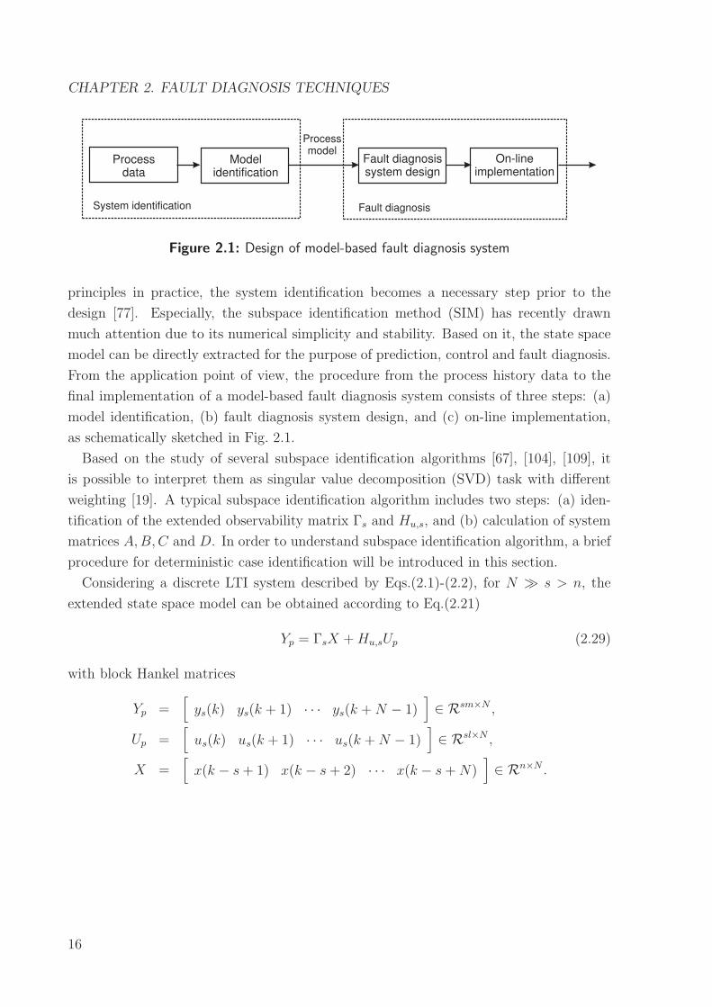
Figure 2.1: Design of model-based fault diagnosis system

principles in practice, the system identification becomes a necessary step prior to the

design [77]. Especially, the subspace identification method (SIM) has recently drawn

much attention due to its numerical simplicity and stability. Based on it, the state space

model can be directly extracted for the purpose of prediction, control and fault diagnosis.

From the application point of view, the procedure from the process history data to the

final implementation of a model-based fault diagnosis system consists of three steps: (a)

model identification, (b) fault diagnosis system design, and (c) on-line implementation,

as schematically sketched in Fig. 2.1.

Based on the study of several subspace identification algorithms [67], [104], [109], it

is possible to interpret them as singular value decomposition (SVD) task with different

weighting [19]. A typical subspace identification algorithm includes two steps: (a) iden-

tification of the extended observability matrix Γs and Hu,s, and (b) calculation of system

matrices A,B,C and D. In order to understand subspace identification algorithm, a brief

procedure for deterministic case identification will be introduced in this section.

Considering a discrete LTI system described by Eqs.(2.1)-(2.2), for N ≫ s > n, the

extended state space model can be obtained according to Eq.(2.21)

Yp = ΓsX +Hu,sUp (2.29)

with block Hankel matrices

Yp =[

ys(k) ys(k + 1) · · · ys(k +N − 1)]

∈ Rsm×N ,

Up =[

us(k) us(k + 1) · · · us(k +N − 1)]

∈ Rsl×N ,

X =[

x(k − s+ 1) x(k − s+ 2) · · · x(k − s+N)]

∈ Rn×N .

16

2.4 Multivariate statistical process monitoring

Introducing ZTp =

[

Y Tp UT

p

]

, the SVD of Zp leads to

Zp =[

U1 U2

]

[

Λ1 O

O Λ2

][

V T1

V T2

]

(2.30)

where Λ2 contains sm− n zero singular values under the assumption that the persistent

excitation condition is satisfied [110]. Straightforwardly, it follows that

U2 =

[

U2,y

U2,u

]

=

[

(Γ⊥s )

T

−HTu,s(Γ

⊥s )

T

]

(2.31)

which indicates that

Γs = (UT2,y)

⊥, (2.32)

−UT2,yHu,s = UT

2,u. (2.33)

According to Eqs.(2.32)-(2.33), the extended observability matrix Γs and the block trian-

gular Toeplitz matrix Hu,s can be simply extracted and the system matrices A,B,C and

D are then identified with the help of the least square method.


In contrast to model-based approaches, in which the quantitative model is known a priori,

the so-called multivariate statistical process monitoring (MSPM) methods are dependent

on large amount of historical data to describe the variability of the process. The most

attractive features of MSPM techniques are easy design and operational simplicity, which

make MSPM more popular in many industrial sectors, especially for detecting the abnor-

mality in large-scale industrial applications [13], [96].

Generally, the basic idea of MSPM techniques is to provide a concise set of statistics

that describes the desired process behavior without direct presentation of huge amount

of raw process data to process engineers. Compared to the univariate methods, which

only monitor the magnitude and variation of single variable, the reliability and robustness

against plant-wide disturbances have been significantly improved. In this section, the basic

MSPM methods, including principal component analysis and partial least squares, will be

briefly introduced in the form of off-line design and on-line implementation algorithms.

2.4.1 Principal component analysis

Principal component analysis (PCA) is a basic method in the framework of MSPM and

originally serves as a dimensionality reduction technique that preserves the significant

17


variability information in the original data set. Since 80’s, PCA has been successfully ap-

plied in numerous areas including data compression, image processing, feature extraction,

pattern recognition and process monitoring [54], [58]. Due to its simplicity and efficiency

in handling huge amount of process data, PCA is recognized as a powerful multivariate

statistical tool and widely used in the process industry for fault detection and diagnosis

[25], [55], [90], [92], [108].

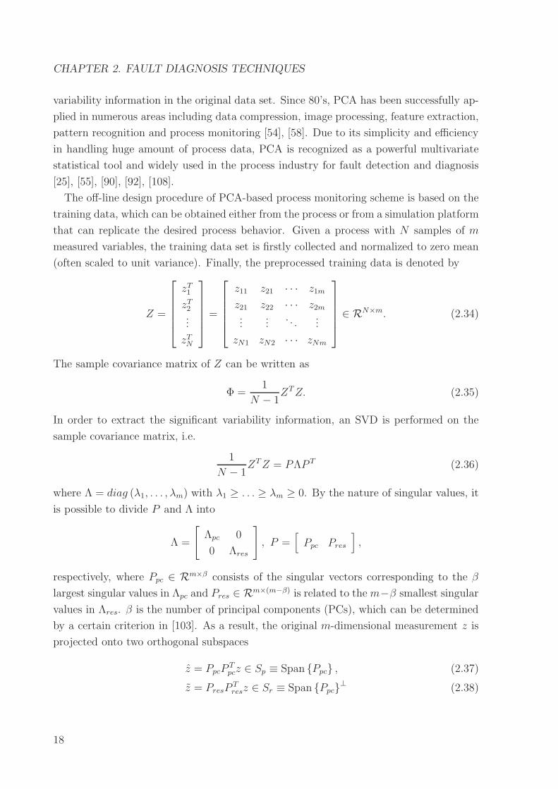
The off-line design procedure of PCA-based process monitoring scheme is based on the

training data, which can be obtained either from the process or from a simulation platform

that can replicate the desired process behavior. Given a process with N samples of m

measured variables, the training data set is firstly collected and normalized to zero mean

(often scaled to unit variance). Finally, the preprocessed training data is denoted by

Z =

zT1zT2...

zTN

=

z11 z21 · · · z1m

z21 z22 · · · z2m...

.... . .

...

zN1 zN2 · · · zNm

∈ RN×m. (2.34)

The sample covariance matrix of Z can be written as

Φ =1

N − 1ZTZ. (2.35)

In order to extract the significant variability information, an SVD is performed on the

sample covariance matrix, i.e.

1

N − 1ZTZ = PΛP T (2.36)

where Λ = diag (λ1, . . . , λm) with λ1 ≥ . . . ≥ λm ≥ 0. By the nature of singular values, it

is possible to divide P and Λ into

Λ =

[

Λpc 0

0 Λres

]

, P =[

Ppc Pres

]

,

respectively, where Ppc ∈ Rm×β consists of the singular vectors corresponding to the β

largest singular values in Λpc and Pres ∈ Rm×(m−β) is related to them−β smallest singular

values in Λres. β is the number of principal components (PCs), which can be determined

by a certain criterion in [103]. As a result, the original m-dimensional measurement z is

projected onto two orthogonal subspaces

z = PpcPTpcz ∈ Sp ≡ Span {Ppc} , (2.37)

z = PresPTresz ∈ Sr ≡ Span {Ppc}

⊥ (2.38)

18


where Span {Ppc} is defined as the set of all linear combinations of the columns in Ppc.

Span {Ppc}⊥ is the orthogonal complement of Span {Ppc}. In order to detect the ab-

normal changes in the both subspaces, the squared prediction error (SPE) [55] and T 2

statistic [102] are computed for on-line implementation. Based on the on-line normalized

measurement sample z, the SPE and T 2 statistics are

SPE = zTPresPTresz, (2.39)

T 2 = zTPpcΛ−1pc P

Tpcz. (2.40)

The thresholds can be calculated for a given confidence level α:

Jth,SPE = θ1

(

cα√

2θ2h20

θ1+ 1 +

θ2h0 (h0 − 1)

θ21

)1/h0

, (2.41)

Jth,T 2 =β (N2 − 1)

N (N − β)Fα (β,N − β) (2.42)

where cα is the normal deviate corresponding to the upper 1−α percentile, F (β,N − β)

stands for F -distribution with β, N − β degrees of freedom and

h0 = 1−2θ1θ33θ22

,

θi =

m∑

j=β+1

(λj)i, i = 1, 2, 3.

Consequently, the fault detection logic follows

SPE ≤ Jth,SPE and T 2 ≤ Jth,T 2 =⇒ fault free, otherwise faulty.

Notice that the basic assumption for applying PCA to process monitoring is that the

measurement variables follow multivariate Gaussian distribution. In addition, the nor-

malization procedure gives same weighting for measurement variables, in which the input

and output relationship has not been considered. However, the correlation between input

and output variables may offer additional advantages for prediction and fault diagnosis.

To this aim, another popular MSPM method, i.e. partial least squares will be introduced

in the next subsection.

2.4.2 Partial least squares

Besides PCA, partial least squares (PLS) is another popular method in MSPM framework

and widely used for model building, fault detection and diagnosis [61], [64], [119]. The

original idea behind PLS is to predict output variables using the on-line observation of

19


process inputs with the help of identified correlation model. For the purpose of process

monitoring, PLS approach is aiming to detect the faults in input measurements which are

mostly related to the output variables. The final outputs in process industry are always

termed as product quality variables and generally can not be measured on-line.

Similar to PCA, the off-line design procedure of PLS-based process monitoring scheme is

based on the training data with process input and output information. Given a normalized

data matrix U which records N samples of l process input variables, and Y consisting of

N samples of m normalized outputs

U =

uT1

uT2...

uTN

∈ RN×l, Y =

yT1yT2...

yTN

∈ RN×m,

ui ∈ Rl, yi ∈ Rm, for i = 1, . . . , N , then PLS involves projection of U and Y onto a low

dimensional space defined by the so-called latent variables (LVs),

T =[

t1 t2 · · · tγ

]

∈ RN×γ

such that the correlation model between U and Y becomes

U = TP T + U = U + U , (2.43)

Y = TQT + Ey = UM + Ey (2.44)

where γ is the number of LVs and P ∈ Rl×γ, Q ∈ Rm×γ are loading matrices of U and

Y , respectively. M ∈ Rl×m is the coefficient matrix. U = TP T is highly correlated with

Y . U and Ey are residual subspaces and assumed to be uncorrelated with Y and U ,

respectively. From the correlation model presented by Eqs.(2.43)-(2.44), the matrix T

and coefficient matrix M can be calculated as

T = UR, (2.45)

M = RQT (2.46)

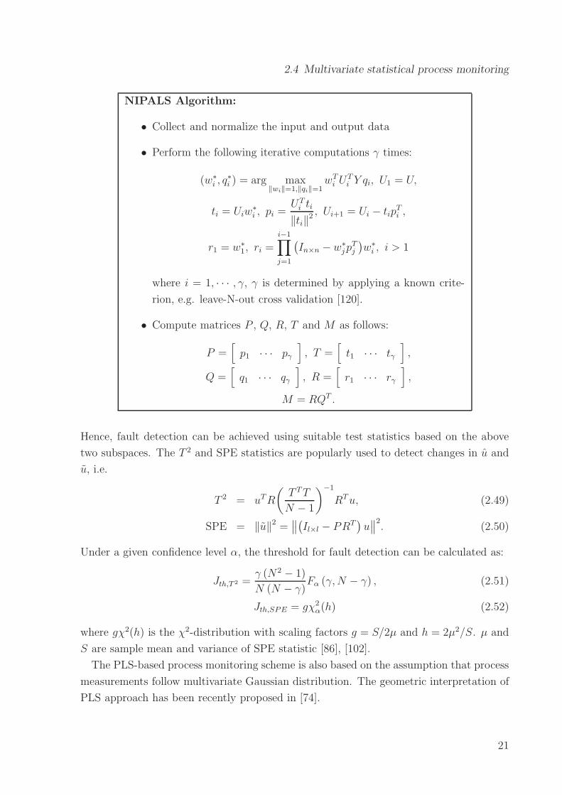
where P TR = RTP = Iγ×γ and R ∈ Rl×γ . The basic PLS algorithm, which is imple-

mented with the so-called nonlinear iterative partial least squares algorithm (NIPALS),

has been summarized in [18], [48], [49].

According to the correlation with outputs, PLS projects input measurement onto the

following two subspaces

u = PRTu ∈ Su ≡ Span {P} , (2.47)

u =(

Il×l − PRT)

u ∈ Su ≡ Span {R}⊥ . (2.48)

20


NIPALS Algorithm:

• Collect and normalize the input and output data

• Perform the following iterative computations γ times:

(w∗i , q

∗i ) = arg max

‖wi‖=1,‖qi‖=1wT

i UTi Y qi, U1 = U,

ti = Uiw∗i , pi =

UTi ti

‖ti‖2 , Ui+1 = Ui − tip

Ti ,

r1 = w∗1, ri =

i−1∏

j=1

(

In×n − w∗jp

Tj

)

w∗i , i > 1

where i = 1, · · · , γ, γ is determined by applying a known crite-

rion, e.g. leave-N-out cross validation [120].

• Compute matrices P , Q, R, T and M as follows:

P =[

p1 · · · pγ

]

, T =[

t1 · · · tγ

]

,

Q =[

q1 · · · qγ

]

, R =[

r1 · · · rγ

]

,

M = RQT .

Hence, fault detection can be achieved using suitable test statistics based on the above

two subspaces. The T 2 and SPE statistics are popularly used to detect changes in u and

u, i.e.

T 2 = uTR

(

T TT

N − 1

)−1

RTu, (2.49)

SPE = ‖u‖2 =∥

∥

(

Il×l − PRT)

u∥

∥

2. (2.50)

Under a given confidence level α, the threshold for fault detection can be calculated as:

Jth,T 2 =γ (N2 − 1)

N (N − γ)Fα (γ,N − γ) , (2.51)

Jth,SPE = gχ2α(h) (2.52)

where gχ2(h) is the χ2-distribution with scaling factors g = S/2µ and h = 2µ2/S. µ and

S are sample mean and variance of SPE statistic [86], [102].

The PLS-based process monitoring scheme is also based on the assumption that process

measurements follow multivariate Gaussian distribution. The geometric interpretation of

PLS approach has been recently proposed in [74].

21


2.4.3 Recent developments on MSPM

PCA and PLS are the most widely accepted data-driven process monitoring methods in

MSPM framework. The standard PCA and PLS algorithms require that the process is

linear and static. The dynamic PCA (DPCA) and dynamic PLS (DPLS) are natural

extensions of the both methods to deal with process dynamics, which can be roughly

expressed in terms of the serial correlations of process variables [16], [66]. In order to

cope with the nonlinearity issue, the kernel-based approaches are also intensively studied

these days [15], [71].

The other MSPM techniques like fisher discriminant analysis (FDA) and independent

component analysis (ICA), are also frequently used in industrial applications. FDA is a

dimensionality reduction technique and has been well studied in the fields of multivariate

statistic and pattern classification [33], [81]. Due to its ability to discriminate among

classes of data, FDA is recognized as an efficient tool for fault classification [12], [14],

[46]. In addition, by defining an additional class of data to represent normal operating

conditions, FDA can also be applied for fault detection purpose [13]. For ICA approach,

the basic idea is to find out the hidden statistically independent components (ICs) from

the observed data. ICA approach is originally proposed to solve the signal processing as

well as blind source separation problems [44], [51], [73]. Recently, ICA has been applied

for process monitoring, especially for the process measurements with non-Gaussian dis-

tributions [60], [72], [70], [133]. Compared with PCA and PLS, the calculation involved

in ICA is more complicated. However, it is worthy of further discussion whether the

independence between the latent variables could bring additional advantage for the eval-

uation stage. Although more sophisticated variants of these methods have been recently

proposed to deal with different issues in industrial processes, a simple method without

complicated computations is still of great interest from the application viewpoint in order

to reduce the design and engineering efforts.

2.5 Concluding remarks

This chapter offers a brief introduction to the major developments and basic concepts of

fault diagnosis techniques, which include model-based and data-driven MSPM approaches.

Depending on the availability of system model, the model-based techniques, such as FDF,

DO and parity space approach, as well as their interconnections are discussed in detail.

Since the process model is hard to be established in practice, the subspace model identi-

fication techniques can be applied to extract the model from process data.

In the second part of this chapter, the data-driven MSPM approaches are briefly in-

22


troduced with the help of PCA and PLS. Compared with model-based techniques, the

data-driven MSPM approaches try to extract a concise set of statistics from huge amount

of process data and hence receive more attention in large-scale process industry nowadays.

Based on the experiences from industrial and research projects, it is observed that some

modifications on basic MSPM approaches are often helpful to improve the process mon-

itoring performance under ideal stationary operating conditions. Moreover, alternative

solutions, which combine the advantages of model-based and MSPM techniques, will lead

to additional improvements on their applicability, capacity and efficiency for industrial

applications. These issues will be discussed in the next four chapters.

23

3 Modifications on PCA-based

approach

The efficiency of PCA-based fault diagnosis scheme lies in its ability to compress a huge

amount of process data and extract the meaningful information within. From application

point of view, the PCA-based fault diagnosis technique is suitable for the processes with

little or no a priori knowledge about their mathematical models. Several extensions of

standard PCA approach have been developed to deal with parameter variations [35], [76]

and industrial batch processes [10], [57], [71], [123]. Although more sophisticated variants

of PCA are proposed, some basic issues of PCA, such as the original idea, test statistics

and their sensitivities to the faults, have not been paid enough attention in research study.

It is well-known that the original idea behind PCA is to reduce the dimension of a data

set, while retaining significant variability information. However, for fault diagnosis, PCA

offers no reduction from the computation point of view since the data should be projected

onto the both subspaces as shown in Eqs.(2.37)-(2.38). In this sense, the core of the PCA-

based approach consists in a numerically reliable implementation of the test statistics

for fault detection, which is mainly achieved based on the SVD. To achieve optimal

fault detection performance, the thresholds of related test statistics shall be delivered by

suitable methods.

In the present work, a new test statistic is firstly proposed. In comparison with the

SPE index, the threshold setting associate with the new statistic is considerably less

complicated than the one given in Eq.(2.41). The further study is dedicated to the

analysis of fault sensitivity. The fault identification issue is finally solved in the proposed

framework [25], [126].

3.1 Problem formulation

The basic assumption on PCA-based fault diagnosis method is that the process variables

follow multivariate Gaussian distribution. Without loss of generality, the measurement

vector can be described as z ∼ N (0,Φ) due to the mean center procedure. The projections

of z onto Ppc and Pres are shown in Eqs.(2.37)-(2.38) such that z = z + z with P Tpcz ∼

24

3.2 On the test statistic

N (0,Λpc) and P Tresz ∼ N (0,Λres). In order to simplify the following study, throughout

this thesis, it is assumed that the sample number N is large enough so that the χ2-

distribution can be adopted instead of F -distribution. The threshold for T 2 statistic can

be calculated as

Jth,T 2 = χ2α(β) (3.1)

where α is confidence level and β is number of PCs. A natural way to monitor the

subspace spanned by Pres is to use the so-called Hawkin’s statistic

T 2H = zTPresΛ

−1resP

Tresz (3.2)

which is, however, less utilized in practice due to the drawback with the possible ill-

conditioning Λres when some of the singular values of λβ+1, . . . , λm are very close to zero.

To solve the problem, the SPE statistic [55] in the form of Eq.(2.39) is proposed with

the threshold given in Eq.(2.41), which is derived from statistical approximation with

complicated computation.

For process monitoring, the offset and scaling faults are the two types of faults which

are mostly considered both in the academic study and practical application. Given a

measurement sample z, the offset and scaling faults can be formulated as follows:

zf = z + f, f 6= 0, (3.3)

zF = Fz, F 6= I (3.4)

where f ∈ Rm and F ∈ Rm×m are constant fault vector and matrix, respectively. Al-

though a successful application of the PCA-based fault diagnosis method depends on the

suitable test statistics for both subspaces, their sensitivities for detecting both types of

faults have not been analytically studied. To complete the entire fault diagnosis scheme,

the fault identification issue shall be finally taken into consideration. Based on the above

observations, this chapter mainly focuses on the following topics:

• Propose suitable test statistic and threshold to monitoring subspace spanned by

Pres,

• Analyze the sensitivity of related test statistic to the fault and,

• Develop an effective fault identification algorithm.


The test statistic plays an important role in PCA-based fault diagnosis technique. Under

given probability density function of the considered variable, the test statistic is utilized to

25

CHAPTER 3. MODIFICATIONS ON PCA-BASED APPROACH

detect the change within. The likelihood ratio methods [4] are popularly used in practice

for the purpose of change detection. Some essentials are introduced in the next subsection.

3.2.1 Generalized likelihood ratio

Given the system model

y = ε+ θ, θ =

{

θ0, no change

θ1, change

where y, θ, ε ∈ Rm, ε ∼ N (0,Σ) and θ is a constant vector. The probability density

function of Gaussian vector y is defined by

pθ,Σ(y) =1

√

(2π)m det(Σ)e−

12(y−θ)TΣ−1(y−θ).

The log likelihood ratio for given vector y satisfies

s(y) = lnpθ1(y)

pθ0(y)=

1

2

[

(y − θ0)TΣ−1(y − θ0)− (y − θ1)

TΣ−1(y − θ1)]

.

The basic idea of likelihood ratio method can be clearly seen from the following decision

rule

s(y) =

{

< 0, θ = θ0 is accepted

> 0, θ = θ1 is accepted.

In statistical framework, s(y) > 0 means pθ1(y) > pθ0(y), i.e. given y, the probability of

θ = θ1 is higher than the one of θ = θ0. Under the assumption that θ0 = 0 and N samples

of y, i.e., y1, . . . , yN , are available, the likelihood ratio is defined by

SN1 =

1

2

[

N∑

k=1

yTk Σ−1yk −

N∑

k=1

(yk − θ1)TΣ−1 (yk − θ1)

]

=1

2

[

N∑

k=1

yTk Σ−1yk −

N∑

k=1

yTk Σ−1yk −N

(

θT1 Σ−1θ1 −

2θT1 Σ−1

N

N∑

k=1

yk

)]

=1

2

[

NyTΣ−1y −N(y − θ1)TΣ−1 (y − θ1)

]

(3.5)

where y = 1N

N∑

k=1

yk. Generally, θ1 is unknown in practice. In order to detect the change

in θ, the so-called generalized likelihood ratio (GLR) is developed. The basic idea of GLR

is to estimate θ1 with maximum likelihood estimation. The maximum likelihood estimate

of θ1 is achieved if the likelihood ratio described in Eq.(3.5) is maximized, which leads to

the solution of the following optimization problem

θ1 = argmaxθ1

SN1 = y =⇒ max

θ1SN1 =

N

2yΣ−1yT .

26


It is of practical interest to notice that the maximum likelihood estimate of θ1 is the

estimate of the mean value of y based on the available samples. Since y ∼ N (0,Σ/N), it

is obvious that NyΣ−1yT follows χ2-distribution. Therefore, given a confidence level α,

the following algorithm can be used for GLR-based change detection.

GLR-based change detection algorithm:

• Determine χα(m) using the table of χ2-distribution with m de-

grees of freedom under confidence interval α

• Set threshold Jth = χα(m)

• Define testing statistic

J = NyΣ−1yT (3.6)

with y = 1N

N∑

k=1

yk

• Define detection logic

J =

{

< Jth, no change

> Jth, a change is detected.

3.2.2 An alternative test statistic

The PCA approach decomposes the measurement space into the so-called principal com-

ponent subspace and residual subspace, which are spanned by Ppc and Pres, respectively.

Since a fault may appear in one of these subspaces, projections of z onto both Ppc and Pres

presented by Eqs.(2.37)-(2.38) should be applied for the fault detection purpose. Note

that T 2 and SPE statistics are of quadratic forms associated with z and z, respectively.

For a fixed sample number N , the GLR test statistic given by Eq.(3.6) leads to an optimal

fault detection performance. It is evident that the T 2 index is exact GLR test statistic

with N = 1 and thus delivers an optimal fault detection performance for the principal

component subspace.

For the residual subspace, the Hawkin’s statistic of Eq.(3.2) can not be directly utilized

due to the possible ill-conditioning of Λres. To avoid this difficulty and also to make use

of easy χ2-distribution table, an alternative statistic is introduced below.

Let

Ξ = diag

(

λm

λβ+1, · · · ,

λm

λm−1, 1

)

∈ R(m−β)×(m−β).

27


It turns out that

Ξ1/2P Tresz ∼ N

(

0, λmI(m−β)×(m−β)

)

and

zTPresΞPTresz = λmz

TPresΛ−1resP

Tresz.

An alternative statistic and the associated threshold are proposed under given confidence

level α

T 2new = zTPresΞP

Tresz, (3.7)

Jth,T 2new

= λmχ2α (m− β) (3.8)

which deliver an optimal fault detection performance in the residual subspace.

It is necessary to point out that

• the new statistic T 2new is equivalent to Hawkin’s statistic T 2

H but without the numer-

ical problem,

• unlike the conventional SPE statistic, whose threshold is derived by statistical ap-

proximation, the new statistic T 2new follows χ2-distribution and the associate thresh-

old can be exactly determined by using the χ2-distribution table, and

• the computation given in Eq.(3.8) is considerably less complicated than the one of

conventional SPE threshold.

Since the principal component subspace and residual subspace are mutually orthogonal,

the fault occurred in one of them can not be detected by the test statistic developed for

the other subspace. In order to ensure high fault detectability, the so-called combined

index [90], [92], which makes simultaneously use of both statistics, is generally formulated

as

T 2c = β1T

2 + β2T2res (3.9)

with known constants β1, β2 > 0. Rewrite Eq.(3.9) into

T 2c = zTPΨP Tz

where

Ψ =

[

β1Λ−1pc 0

0 β2Q

]

, Q =

Λ−1res, T 2

res = T 2H

I, T 2res = SPE

Ξ, T 2res = T 2

new

.

28

3.3 Fault sensitivity analysis

Considering that P Tz ∼ N (0,Λ), zTPΛ−1P Tz ∼ χ2(m), it is reasonable to introduce the

following combined statistic to avoid possible difficulty with the computation of Λ−1

T 2comb = zTP ΞP Tz with Ξ = diag

(

λm

λ1, · · · ,

λm

λm−1, 1

)

(3.10)

which is a combined index T 2comb = λm(T

2 + T 2H). For a given confidence level α, the

threshold of T 2comb is given by

Jth,comb = λmχ2α (m) . (3.11)

The combined index can also be interpreted as a weighted quadratic form of the obser-

vation projection P T z. It is interesting to notice that the direction coupled with a stronger

variance is less weighted, while the direction with a weaker variance has a stronger weight-

ing.

In the extreme case that the sample covariance matrix Φ is singular, an SVD yields

Φ =1

N − 1ZTZ =

[

P P⊥

]

[

Λ 0

0 0

][

P T

P T⊥

]

.

As a result, the fault detection can be achieved by using the combined index in Eq.(3.10)

with the associated threshold Eq.(3.11) and the parity checking

P T⊥ z = 0. (3.12)

The corresponding detection logic is

T 2comb ≤ Jth,comb and (3.12) is true =⇒ fault free, otherwise a fault is detected.


In this section, the fault sensitivity of the related test statistic will be analyzed. Recall-

ing the offset and scaling faults defined in Eqs.(3.3)-(3.4), the scaling fault can also be

formulated as a special kind of offset fault in case of

f = F − Im×mz.

Therefore, in the sequent study of fault sensitivity analysis, the general form of fault is

considered as

zf = z + f.

Since T 2H , T

2new and SPE are equivalent to represent test statistic for residual subspace, in

the following analysis T 2res is formulated by T 2

H to simplify the notation. Similarly, T 2comb

represents the combined index T 2c .

29


3.3.1 Comparison between T 2 and T 2res statistics

According to the nature of fault, two cases are considered as follows.

• Fault occurs in Ppc or Pres. In this case, the T 2 and T 2res statistics are only sensitive

to the faults which can be decomposed into subspaces spanned by Ppc and Pres,

respectively. Since the principal component subspace and residual subspace are

mutually orthogonal, if a fault occurs only in Ppc (or Pres), the T2res (or T

2) statistic

will never detect the fault regardless of its magnitude.

• Fault has the similar influences on both subspaces. Since the covariance matrices of

P Tpcz and P T

resz are, respectively, Λpc and Λres, and furthermore λmin(Λpc) = λβ ≫

λmax(Λres) = λβ+1, the T 2res statistic may be more sensitive to the fault than T 2

statistic. To demonstrate it, the fault sensitivity of related test statistic will be

analytically studied in this subsection.

For a confidence level α, it follows that

maxz∈N (0,Φ)

(

zTPresΛ−1resP

Tresz)

≤ Jth,T 2H= X 2

α(m− β),

maxz∈N (0,Φ)

(

zTPpcΛ−1pc P

Tpcz)

≤ Jth,T 2 = X 2α(β).

Thus, if a fault f causes

(

fTPresPTresf

)1/2> 2λ

1/2β+1J

1/2

th,T 2H

= 2λ1/2β+1

(

X 2α(m− β)

)1/2, (3.13)

it becomes

(

zTf PresΛ−1resP

Treszf

)1/2≥

(

fTPresΛ−1resP

Tresf

)1/2−(

zTPresΛ−1resP

Tresz)1/2

≥ λ−1/2β+1

(

fTPresPTresf

)1/2− J

1/2

th,T 2H

> J1/2

th,T 2H

which means this fault can be detected with the confidence level α. Note that Eq.(3.13)

is a sufficient condition under that a fault can be detected by T 2H . On the other hand, it

is obvious that

E(

T 2)

= E(

zTf PpcΛ−1pc P

Tpczf

)

= E(

zTPpcΛ−1pc P

Tpcz)

+ fTPpcΛ−1pc P

Tpcf

≤ E(

zTPpcΛ−1pc P

Tpcz)

+ λ−1β fTPpcP

Tpcf

= β +λβ+1f

TPpcPTpcf · λ−1

β+1fTPresP

Tresf

λβfTPresP Tresf

.

30


According to Eq.(3.13), it is known that

λ−1β+1f

TPresPTresf = 4Jth,T 2

H+ δ, (3.14)

(

fTPresPTresf

)1/2> 2λ

1/2β+1J

1/2

th,T 2H

(3.15)

with δ > 0. In case that the fault has similar influence on the both subspaces, i.e.

fTPpcPTpcf ≈ fTPresP

Tresf, (3.16)

it turns out

E(

zTf PpcΛ−1pc P

Tpczf

)

≤ β +λβ+1 (4χ

2α(m− β) + δ)

λβ.

In caseλβ+1

λβ≤

X 2α(β)− β

4X 2α(m− β) + δ

, (3.17)

it follows that

E(

zTf PpcΛ−1pc P

Tpczf

)

≤ X 2α(β) = Jth,T 2 (3.18)

which indicates that f is expectably undetected by the T 2 statistic under condition in

Eq.(3.17), although it is detectable using the Hawkin’s T 2H statistic. Since generally

4X 2α(m − β) and X 2

α(β) − β are comparable and the singular values λβ ≫ λβ+1, the

condition Eq.(3.17) is a general condition and easy to satisfy.

The previous analysis reveals that T 2res is more sensitive to the fault than the T 2 statistic

when the fault has the same influence on both subspaces.

3.3.2 On the combined index

In this subsection, the sensitivity of combined index will be analyzed. It is straightforward

that, for a fault occurred in Ppc, it will cause same change in T 2 and T 2c . Note that the

threshold of T 2c can be calculated by χ2

α (m). In addition, since

χ2α (m) > χ2

α (β) ,

χ2α (m) > χ2

α (m− β) ,

the combined index has lower fault sensitivity than the separate use of T 2. The similar

analysis can be applied on the fault occurred in the residual subspace that delivers the

same result.

On the other hand, it always holds

χ2α (m) < χ2

α (m− β) + χ2α (β) .

31


Thus, there must exist a fault which leads to

T 2c > χ2

α (m)

under the following conditions

T 2 < χ2α (β) ,

T 2res < χ2

α (m− β) .

In this case, the combined index may be more sensitive to the fault than using the separate

indices.

The previous discussion reveals that

• if the fault f has significantly different influences on the both subspaces, i.e. one of

the following two conditions is satisfied

fTPpcPTpcf ≪ fTPresP

Tresf,

fTPpcPTpcf ≫ fTPresP

Tresf.

The separate use of the two test statistics, T 2 and T 2res, will improve the fault

sensitivity compared with the combined index, and

• the use of a combined index is of advantage when the distribution of Λ−1f is nearly

uniform in the measurement subspace.

According to these observations, each index, i.e. T 2, T 2res or T 2

c , can be sensitive to a

certain kind of faults. Therefore, the joint use of the related test statistics is recommended

to improve the fault detection performance.

3.4 Fault identification

The fault sensitivity analysis of related test statistic has been discussed so far. In this

framework, the issues of identification of off-set and scaling faults will be respectively

considered.

3.4.1 Identification of off-set fault

As aforementioned, the off-set fault is given by

zf = z + f, f 6= 0

32

3.4 Fault identification

where z ∼ N (0,Φ), Φ is a known matrix and f is an unknown constant vector. It is well

known that

zf =1

N

N∑

i=1

zf,i

delivers a GLR estimate for f , where zf,i (i = 1, · · · , N) is the i-th sample of zf . Suppose

that a fault is detected with sample k, the off-set fault identification procedure can be

briefly summarized as follows: Collect M faulty samples and compute the estimate of f ,

denoted by f , as

f =1

M + 1

k+M∑

i=k

zf,i. (3.19)

In case that the nominal measurement vector is not zero mean, the M faulty samples

shall be firstly centered by the mean value achieved from the training data. Based on the

re-centered samples, Eq.(3.19) can be utilized to estimate the off-set fault. It is worth to

mention that the above algorithm can also be realized in a recursive manner.

3.4.2 Identification of scaling fault

Consider a scaling fault

zF = Fz, F 6= I,

and suppose that the fault has been detected by standard PCA method with sample k.

Let zF,k, · · · , zF,k+M be M + 1 samples collected after fault detection. Then, it follows

that

1

M

[

zF,k · · · zF,k+M

]

zTF,k...

zTF,k+M

≈ FΦF T = FPΛP TF T . (3.20)

An SVD on Eq.(3.20) leads to

1

M

[

zF,k · · · zF,k+M

]

zTF,k...

zTF,k+M

= V ΠV T (3.21)

with Π = diag(

λ1, · · · , λm

)

. Straightforwardly, it follows

V Π1/2 = FPΛ1/2.

In case that Λres ≈ 0, the pseudo inverse of PΛ1/2 is given by

(

PΛ1/2)†

≈

[

Λ−1/2pc 0

0 0

][

P Tpc

P Tres

]

.

33


The estimate of F , denoted by F , can be calculated by

F = V1Π1/2pc Λ−1/2

pc P Tpc (3.22)

where

Πpc = diag(

λ1, · · · , λβ

)

,

Πpc contains β significant singular values in Π and V1 are the corresponding singular

vectors.

3.4.3 A fault identification algorithm

Assume that a fault has been detected by using T 2, T 2res or T 2

c at sample k. The major

results achieved in this section can be summarized into the following algorithm.

Fault identification algorithm:

• Collect M +1 faulty samples and center them by the mean value

achieved from training data

• Estimate the off-set fault using Eq.(3.19)

• Re-center the samples by f

• Perform the SVD on Eq.(3.21) based on the re-centered samples

• Compute F according to Eq.(3.22).


This chapter mainly focuses on the modifications on standard PCA-based fault diagnosis

approach. Based on the review of GLR method, a new test statistic for residual subspace

is proposed, which is equivalent to the Hawkin’s T 2H statistic but without numerical draw-

backs. In comparison with standard SPE statistic, the threshold calculation associated

with the proposed test statistic is remarkably simple and does not need statistical approx-

imation. A modified combined index is also developed based on the new test statistic.

The further study is dedicated to evaluating these test statistics according to their sensi-

tivities to the fault. As a result, the joint use of these test statistics is recommended. To

complete the fault diagnosis framework, an algorithm is finally proposed to identify the

off-set and scaling faults.

34


Unlike the original idea of PCA, which is to reduce the dimension of data by retaining

significant variations, both of the principal component subspace and residual subspace

should be utilized to achieve reliable fault detection performance. The core of the PCA-

based approach consists in a numerically reliable implementation of the χ2 test for fault

detection, which is mainly achieved using the SVD.

35

4 Modifications on PLS-based

approach

Besides PCA, PLS is another popular method in MSPM framework. In contrast to PCA,

which gives the same weighting to each process variable without considering any causal

relationship in the process, PLS extracts the correlation model between process inputs and

outputs that may provide further advantages for prediction and fault diagnosis purposes.

Although both methods perform a similar way for fault detection, the main aim of PLS is

to detect the changes in input variables that are mostly influential to the process outputs

by utilizing the correlation information. The basic concepts and algorithms of PLS can

be found in [48], [49]. Several modifications of it, such as recursive PLS [89], multiblock

PLS [69], [80], local PLS [65] and dynamic PLS [16] are also proposed and implemented

in a variety of industrial applications.

Although PLS-based fault diagnosis technique has been widely used, less attention has

been paid to the property of the latent space for fault diagnosis purpose. As shown

by Eqs.(2.47)-(2.48), the standard PLS algorithm decomposes the input measurement

space into two oblique subspaces which may cause some problems for fault diagnosis.

Moreover, the standard PLS algorithm introduced in Subsection 2.4.2 is computationally

complicated, and most importantly, the correlation model is difficult to interpret due to

many iterative computational steps caused by the large number of latent variables.

Motivated by aforementioned observations, in the present work, a modified approach

is firstly proposed in order to overcome these difficulties [129]. Based on it, the complete

process monitoring scheme is further designed. To this end, a brief comparison between

the proposed method and existing approaches is given. Notice that the similar procedure

introduced in Section 3.4 can also be utilized for fault identification.


It is known that standard PLS algorithm divides input measurement space, U , into two

subspaces, i.e. U and U , depending on their correlation with output variables, Y . Based

on it, the T 2 and SPE statistics are typically used for monitoring both subspaces. Al-

36

4.2 A modified approach

though standard PLS algorithm works in many cases, the complexity of algorithm, es-

pecially the iterative computation procedures caused by many latent variables, lead to

the PLS model to be difficult to explain. In addition, it reveals that the standard PLS

approach may result in partial correlation between U and Y thus, the orthogonal varia-

tions in U are useless for outputs prediction. Moreover, U may contain large variability

of U and therefore, is not suitable for monitoring as residual subspace by means of SPE

statistic. To solve these problems, Zhou et al. [134] proposed the so-called total projection

to latent structure (TPLS) approach, which is based on the results from standard PLS

algorithm and further performs decomposition on certain subspaces.

The drawback due to orthogonal variations amongst interacting subspaces comes from

the nature of the standard PLS algorithm. Hence, a slight modification is necessary

in order to achieve better fault diagnosis performance. From the application point of

view, a desired modification approach shall be computationally less expensive than the

standard one and more importantly, avoid the drawbacks mentioned earlier. As a result,

the following two issues must be resolved:

• Perform a complete decomposition on input and output spaces, such that the cor-

relation model becomes

U = U + U , (4.1)

Y = Y + Ey, (4.2)

Y = UM = UM (4.3)

where the subspaces Y and Ey are respectively correlated and uncorrelated with

the input space. U and U denote an orthogonal decomposition on input space such

that U has no contribution for outputs prediction, while U is fully responsible for

predicting Y thus does not contain variations orthogonal to Y , and

• Develop suitable test statistics and fault identification algorithm to complete the

fault diagnosis scheme.

To deal with the first issue, a modified approach is derived in the next section.


4.2.1 A complete decomposition of Y space

Based on the discussion so far, it is possible to write the desired relation as follows

Y = UM + Ey = Y + Ey (4.4)

37

CHAPTER 4. MODIFICATIONS ON PLS-BASED APPROACH

where M is the coefficient matrix and contains correlation information between U and Y .

Ey is the residual part of Y which is uncorrelated with the input measurement, i.e.

cov (ey, u) = 0

where uT and eTy are row vectors in U and Ey, respectively. Without the loss of generality,

M is assumed to be a full column-rank matrix. According to Eq.(4.4), in case of N ≫

max {l, m}, it follows that

1

N − 1Y TU =

1

N − 1MTUTU +

1

N − 1Ey

TU ≈ MT UTU

N − 1.

Thus, if matrix UTU is invertible, M can be easily calculated as:

M =(

UTU)−1

UTY. (4.5)

Note that, if the product UTU is not a full rank matrix, it follows that

M =(

UTU)†UTY. (4.6)

The pseudo inverse is calculated as:(

UTU)†

= Pu,pcΛ−1u,pcP

Tu,pc (4.7)

where an SVD on UTU leads to

UTU = PuΛuPTu =

[

Pu,pc Pu,res

]

[

Λu,pc 0

0 Λu,res

][

P Tu,pc

P Tu,res

]

(4.8)

with Λu,res = 0. It is now easy to show that Y is completely decomposed into two parts

as desired in Eq.(4.4) depending on their correlations with input measurement space.

4.2.2 Orthogonal decomposition of U space

So far, a desired decomposition on Y has been achieved and based on this result, it is

necessary to decompose U into two parts, i.e. U and U , such that U does not contain

variations orthogonal to Y and thus has the full contribution in predicting Y , while U

gives no contribution.

A simple way to perform the aforementioned decomposition is achieved by projecting

U orthogonally onto the subspaces Su ≡ span {M} and Su ≡ span{M}⊥, respectively.

Consequently, it follows that

UM = 0, (4.9)

Y = UM = UM, (4.10)

U ∈ Su, U ∈ Su. (4.11)

For orthogonal projection, the following steps are necessary:

38


• Perform the SVD on matrix MMT

MMT =[

PM PM

]

[

ΛM 0

0 0

][

P TM

P TM

]

(4.12)

with PM ∈ Rl×m, PM ∈ Rl×(l−m), ΛM ∈ Rm×m.

• Construct ΠM , Π⊥M , which are the orthogonal projectors of the subspaces Su and

Su respectively, i.e.

ΠM = PMP TM , (4.13)

Π⊥M = PM P T

M . (4.14)

• Project U onto subspaces Su ≡ span {M} and Su ≡ span{M}⊥, which are mutually

orthogonal. Hence, U is decomposed into two parts, i.e.

U = U + U (4.15)

such that

U = UΠM = UPMP TM ∈ Su ≡ span {M} , (4.16)

U = UΠ⊥M = UPM P T

M ∈ Su ≡ span{M}⊥. (4.17)

The major results achieved in this section can be summarized as the following algorithm.

Table 4.1 provides the descriptions of related subspaces.

Algorithm of the modified approach

• Calculate the coefficient matrix M according to Eq.(4.5) or

Eq.(4.6)

• Do an SVD on MMT , see Eq.(4.12)

• Calculate the orthogonal projectors by Eqs.(4.13)-(4.14)

• (optional) Decompose U according to Eqs.(4.15)-(4.17)

• (optional) Decompose Y as Y = UM , Ey = Y − Y .

39


Table 4.1: Description of subspaces

Subspace Description

Usubspace of U that is fully responsible for

predicting Y

Usubspace of U that is orthogonal to U and

has no contribution for prediction of Y

Ysubspace of Y that is correlated to U and represents

the prediction of outputs

Ey subspace of Y that is uncorrelated to U

It is worth to point out that

• the proposed approach calculates the coefficient matrix M in a least square manner

and based on it, the orthogonal decomposition on the input space is performed,

• compared to the standard PLS algorithm, the proposed approach provides a desired

decomposition on input and output spaces as shown in Eqs.(4.1)-(4.3), and thus

avoids the drawbacks of standard PLS algorithm, and

• the proposed approach provides a more clear interpretation of the correlation model

and has much less computational overload than the standard PLS algorithm.

4.3 The fault defection scheme

Based on the proposed approach, in this section, the fault detection scheme will be dis-

cussed in detail.

4.3.1 Monitoring subspace U

Since U and Y are mutually correlated, it is easy to prove that they are equivalent in the

sense of change detection. Thus, in this subsection, the issue of monitoring on subspace U

is mainly studied, which enables detecting the fault in the input space that has influence on

the outputs. To this end, consider the quadratic form of vector u, which is recommended

40

4.3 The fault defection scheme

to design the test statistic:

uT u = uTPMP TMPMP T

Mu = uTPMP TMu. (4.18)

Since

rank{

P TMUT

}

= m,

P TMu ∈ Rm is a suitable candidate for T 2 statistic for monitoring U . Thus, the T 2 statistic

follows

T 2u = uTPM

(

P TMUTUPM

N − 1

)−1

P TMu. (4.19)

The threshold for T 2u is given by

Jth,T 2u=

m (N2 − 1)

N (N −m)Fα (m,N −m) (4.20)

where F (m,N −m) is F -distribution with m and N − m degrees of freedom and α is

user-specified confidence level. Recalling the GLR technique, in case of large enough N ,

the threshold for T 2u can be determined by χ2 test instead of F -distribution as shown in

Eq.(4.20), i.e.

Jth,T 2u= χ2

α(m). (4.21)

The fault detection logic is:

T 2u > Jth,T 2

u=⇒ a fault in inputs is detected that is influential on outputs.

4.3.2 Monitoring subspace U

As mentioned in the previous section, U represents a subspace in U that is not correlated

to Y and has no contribution for output prediction. Therefore, similar to Eq.(4.18), the

quadratic form of u can be written as:

uT u = uT PM P TM PM P T

Mu = uT PM P TMu. (4.22)

Noting that

rank{

P TMUT

}

= l −m,

hence, P TMu ∈ Rn−m can be used as T 2 statistic for monitoring U . Thus, it follows

T 2u = uT PM

(

P TMUTUPM

N − 1

)−1

P TMu. (4.23)

The threshold for T 2u is

Jth,T 2u=

(l −m) (N2 − 1)

N (N − l +m)Fα (l −m,N − l +m) (4.24)

41


where F (l −m,N − l +m) is F -distribution with l−m and N− l+m degrees of freedom

under confidence level α. Similarly, the threshold can be determined by Jth,T 2u= χ2

α(l−m).

The fault detection logic is

T 2u > Jth,T 2

u=⇒ a fault in inputs is detected without influence on outputs.

4.3.3 Monitoring subspace Ey

In this subsection, monitoring and change detection based on Ey is investigated. It is

known that Ey is not correlated to input space and can be represented by

Ey = Y − Y =(

U + U)

M + Ey − UM (4.25)

which shows that Ey is not influenced by any change in input measurement. In other

words, only the faults occurred in Y , e.g. sensor failures, can be detected by monitoring

Ey. Generally, ey is assumed small in magnitude and contains insignificant variability

information. Based on the available measurement y, an SPE statistic can be designed as

SPEy = ‖ey‖2 = ‖y − y‖2 =

∥

∥y −MTu∥

∥

2. (4.26)

The related threshold is

Jth,SPEy= gyχ

2α(hy) (4.27)

where gyχ2(hy) is χ2-distribution with scaling factor gy = S/2µ and hy = 2µ2/S under

given confidence level α. µ and S are sample mean and variance of SPEy statistic in

Eq.(4.26). In case that input measurement is fault free, the fault detection logic is given

as:

SPEy ≤ Jth,SPEy=⇒ fault free, otherwise a fault in y is detected.

Note that, in Subsection 3.2.2, a new test statistic, which is similar to Hawkin’s T 2H statis-

tic but without the numerical drawback, has been proposed instead of SPE. Moreover, if

ey is large and retains significant variability information, the new statistic can be simply

extended to a combined index to ensure high fault detectability. In this case, the test

statistic for Ey becomes

T 2y = eTy PyΞP

Ty ey (4.28)

42

4.4 A brief comparison

Table 4.2: Subspaces and related test statistics

Subspace Test statistics Threshold

U T 2u

m(N2−1)N(N−m)

Fα (m,N −m)

U T 2u

(l−m)(N2−1)N(N−l+m)

Fα (l −m,N − l +m)

Ey T 2y λmχ

2α (m)

where

Ξ = diag

(

λm

λ1

, · · · ,λm

λm−1

, 1

)

,

λ1 ≥ · · · ≥ λβ ≫ λβ+1 ≥ · · · ≥ λm > 0,

Λy,pc = diag(λ1, · · · , λβ), Λy,res = diag(λβ+1, · · · , λm),

1

N − 1ET

y Ey = PyΛyPTy , Λy =

[

Λy,pc 0

0 Λy,res

]

.

Notice that Λy,pc and Λy,res are calculated by the SVD of 1N−1

ETy Ey in the off-line design

phase. The corresponding threshold is

Jth,T 2y= λmχ

2α (m) . (4.29)

The test statistics related to different subspaces are listed in Table 4.2. To this end, it is

necessary to point out that

• the proposed approach employs two T 2 indices to monitor input measurement space.

As against four test statistics proposed in [134], the proposed monitoring scheme

works more efficiently, and

• in practice, the output vector y, e.g. the one serves as product quality variable,

is not always available on-line. In this case, monitoring subspace Ey by means of

SPEy or T 2y will induce time delay and it is usually used in off-line analysis.

4.4 A brief comparison

Table 4.3 offers a brief comparison among the proposed approach, PLS and TPLS [134],

in which the computation complexity of the off-line algorithm, the number of on-line test

statistics as well as design parameters are mainly taken into consideration.

43


Table 4.3: Comparison among PLS, TPLS, modified approach

Method Computation complexity Statistics Parameter

PLSγ times SVD

on l × l matrix2 No. of LVs

TPLSγ + 1 SVD on l × l +

1 SVD on m×m matrices4 No. of LVs

Modified

approach

2 times SVD

on l × l matrix2 no

The computational complexities of these approaches mainly come from the SVD on

covariance matrices with different dimensions. Standard PLS needs γ times SVD on l× l

matrix. TPLS is based on the results from standard PLS algorithm and additionally

needs 2 times SVD on m×m matrix and an SVD on l× l matrix. The computation cost

of the proposed approach mainly comes from 2 times SVD on l × l matrix that shows

relative lower computation cost compared to PLS and TPLS in case of γ > 2.

As aforementioned, for on-line implementation, the PLS and modified approach employ

2 test statistics to monitor the input measurement space, while TPLS has 4 test statistics

for the same purpose. Moreover, it is worth mentioning that the number of LVs, γ, is

an important design parameter in standard PLS to achieve successful process monitor-

ing. The leave-N-out cross validation is mostly referred in the literature for selecting the

number of LVs. Although it is a widely used criterion in practice, different results can

be obtained according to the choice of N , which may finally influence the performance of

the overall fault diagnosis system. Based on this observation, the approach without such

a design parameter will show much more advantages from the application point of view.

4.5 On fault identification issue

Assume that a fault of input measurement has been detected using T 2u or T 2

u . The fault

identification on the input space can be similarly achieved according to the algorithm

presented in Subsection 3.4.3. It is known that, the fault detected by T 2u will finally

influence the output measurement y. Thus, if test statistic T 2y indicates a fault occurred

on y, the influence of faulty input measurement shall be firstly subtracted in order to reflect

the real fault information occurred in outputs. Based on it, the similar fault identification

procedure can be applied to identify the faults in output measurement space. To this end,

44

4.6 Simulation examples

a brief algorithm can be summarized as follows.

Fault identification algorithm:

• Assume that a fault on input measurement is detected by T 2u or

T 2u at time sample k

• Utilize the fault identification procedure presented in Subsec-

tion 3.4.3 to identify the fault in input measurement space

• Suppose a fault on output measurement is also detected by T 2y .

Subtract the influence of the faulty input measurement from the

available output measurement. Thus, the data reflecting the real

faulty information occurred in y are obtained.

• Utilize similar fault identification procedure to identify the fault

in output space.


In this section, the results obtained with an academic example are presented to illustrate

the performance of the modified approach. Consider the following numerical example

[134]:

uk = Azk + ek, (4.30)

yk = Cuk + vk (4.31)

where

A =

1 3 4 4 0

3 0 1 4 1

1 1 3 0 0

T

, C =[

2 2 1 1 0]

,

and the noise terms vk ∼ N (0, 0.01), ek,j ∼ U([0 0.05]) and zk,i ∼ U([0 1]) for i = 1, · · · , 3

and j = 1, · · · , 5. U denotes the uniform distribution.

An additive fault is considered in the following form:

uf = u+ Ξf (4.32)

where u is the fault free process vector, Ξ ∈ Rl×1 denotes fault direction vector and scalar

f is the magnitude of fault.

45


0 50 100 150 2000

10

20

30

40

0 50 100 150 2000

10

20

30

40

T2

u

T2

u

Samples

(a) faults in U

0 50 100 150 2000

10

20

30

40

0 50 100 150 2000

10

20

30

40

T2

u

T2

u

Samples

(b) faults in U

0 50 100 150 2000

0.5

1

1.5

2

2.5

0 50 100 150 2000

0.5

1

1.5

2

2.5

SPEy (faults in U)

SPEy (faults in U)

Samples

(c) SPEy for faults in U and U

0 50 100 150 2000

5

10

0 50 100 150 2000

5

10

0 50 100 150 2000

1

2

3

T2

u

T2

u

SPEy

Samples

(d) T 2

u, T 2

uand SPEy statistic for faults in output

Figure 4.1: Modified approach based process monitoring

For the experiments, following design steps are carried out:

• Off-line training phase: Collect training data consisting of 1000 samples and perform

the modified approach to calculate M , PM and PM .

• Threshold computation: Compute thresholds for Jth,T 2uand Jth,T 2

uwith N = 1000,

l = 5, m = 1, confidence level α = 0.99. Optionally, compute Jth,SPEy.

• On-line fault detection: Simulate the example given by Eqs.(4.30)-(4.31) for 200

samples with fault occurrence after the 100-th time sample. Three different faults

are considered as follows.

Fault in U : As shown in Eq.(4.32), Ξ is selected as the first column of PM and

46


Table 4.4: Fault detection rate (%): faults in U

Magnitude of f Modified (T 2u) Modified (T 2

u) PLS (T 2) PLS (SPE)

2 8 2 3 5

4 39 2 12 6

6 60 2 24 9

8 75 2 33 15

10 96 2 57 39

Table 4.5: Fault detection rate (%): faults in U

Magnitude of f Modified (T 2u) Modified (T 2

u) PLS (T 2) PLS (SPE)

2 1 21 1 9

4 1 89 1 44

6 1 100 1 97

8 1 100 1 100

10 1 100 1 100

f = 6

Fault in U : Similar to fault in U , Ξ is selected as the first column of PM , f = 6

Fault in Y : Additive fault on output.

Compute T 2u and T 2

u . Optionally, calculate SPEy.

Fig. 4.1(a) shows the result when fault occurs in U , which can be successfully detected

by T 2u without significant influence on T 2

u . On the other hand, Fig. 4.1(b) indicates that if

a fault occurs in U , T 2u crosses the threshold without significant change in T 2

u . Moreover,

as seen from Table 4.4, compared to the standard PLS, the proposed approach not only

offers correct fault location information but also provides significant improvement on

fault detection rate. T 2u gives higher fault detection rate than T 2 and T 2

u gives lower false

alarm rate than SPE statistic of standard PLS approach. Similar results are obtained for

fault occurred in U as shown by Table 4.5. In addition, if the fault occurred in input

measurement space, SPEy statistic gives no alarm, see Fig. 4.1(c). Fig. 4.1(d) illustrates

T 2u , T

2u and SPEy statistics if faults occurred in output. It can be seen that only SPEy

exceeds the threshold that delivers useful information of the location of the fault.

47



In this chapter, a new approach is proposed to overcome the drawbacks of standard PLS-

based fault diagnosis technique. This approach firstly calculates the coefficient matrix

in a least square manner and then based on it, divides the input measurement into two

orthogonal subspaces according to their correlation with outputs. The proposed approach

is considerably simpler than the standard technique, and most importantly, avoids the

drawbacks and provides a clear interpretation for the correlation model. Based on the

proposed approach, the fault detection scheme is designed, in which only two T 2 statistics

are used for monitoring the overall input space. An algorithm for fault identification is

also included in this study.

48

5 Subspace aided data-driven approach

PCA- and PLS-based fault diagnosis methods are powerful tools to deal with the ap-

plications under the ideal stationary operating conditions. However, in the industrial

applications, we often meet situations that the operating conditions are significantly dif-

ferent from those conditions assumed for the application of the basic MSPM methods.

This issue can be illustrated, e.g. by the schematic description of a typical industrial

batch process presented in Fig. 5.1. It is evident that the basic MSPM methods like PCA

and PLS are not able to construct a reliable fault diagnosis scheme, since

• the process dynamics has not been taken into consideration in the basic MSPM

approaches,

• an explicit model for the internal relations between the process variables and oper-

ating conditions is always not available in practice and,

• the normalization procedure, which serves as a basic step for MSPM methods, is

not suitable for such a process due to wide operation region of process variables.

Although more sophisticated extensions of basic MSPM approaches have been proposed

to deal with such dynamic processes [10], [29], [57], [71], [94], [123], a simple method

Figure 5.1: Schematic description of an industrial batch process

49

CHAPTER 5. SUBSPACE AIDED DATA-DRIVEN APPROACH

without complicated algorithm is still of great interest from the application viewpoint to

reduce the design and engineering efforts.

On the other hand, it is known that the main advantages of the model-based fault

diagnosis methods lie in their abilities to deal with aforementioned problems that ensure

most efficient way for dynamic process monitoring. Unfortunately, their applications are

often unrealistic due to the sophisticated modeling procedure from the first principles,

especially for large-scale industrial process.

An alternative way, which is more simple than construction of process model from the

first principles, is identification of the process model from operation data. For this pur-

pose, SIM techniques that directly identify the complete state space matrices have gained

tremendous attention in the last two decades and have been successfully implemented in

many industrial applications [36], [87], [91]. Provided the identified process model, ob-

server and parity space based FDI schemes can be designed [50], [106], [131]. The block

diagram in Fig.5.2 describes the classic subspace identification aided design for observer-

based fault diagnosis system, in which the state space matrices are identified from the

estimated state sequence and the residual generator based on DO or parity relation is

then designed according to the model-based FDI schemes described in Section 2.2.

In the present work, an alternative procedure is proposed [24]. As illustrated in Fig. 5.2,

the central idea behind the new method is the design of the parameters of DO based on

the primary form of residual generators, whose parameters can be directly identified from

the process data. In this way, the system identification becomes a part of the fault

diagnosis system that leads to a shorter, easier and faster design procedure. A basic

assumption in the proposed design scheme is that the mathematical model of the process

under consideration is not available. This new approach is of significant practical interest

due to the following features:

• The proposed approach is suitable for the application under industrial operating

conditions.

• The design procedure is intuitive yet simple and only based on the measured data

from the process under consideration.

• Primary fault detection can be realized with the minimal set of identified parameters

that is very important and valuable for the application engineers in early project

phase to check the realizability of an FDI scheme.

• No special knowledge of modern control theory is needed for design of observer-based

residual generators.

50

SUBSPACE AIDED DATA-DRIVEN APPROACH

Input and output data

State sequence

System matrices

Parity space

Residual generator

, , , , ,z z z z z zA B L c d g

ˆ, kn x

,k ku y

, , ,A B C D

sP

Classic approach New approach

Subspace technique

Figure 5.2: SIM and new approach

The proposed work is strongly motivated by the successful application of basic MSPM

techniques in process industry but also by the intimate relationship between the SIM and

parity vectors, which has been studied in [3], [41], [75], [93], [110], [111].

51


5.1 Preliminaries on subspace aided approach

5.1.1 Mathematical notations

Assume that the process under consideration can be modeled as an LTI system described

by

x(k + 1) = Ax(k) +Bu(k) + w(k), (5.1)

y(k) = Cx(k) +Du(k) + v(k). (5.2)

The model equations are introduced in Eqs.(2.1)-(2.2) in Chapter 2 with w(k) ∈ Rn,

v(k) ∈ Rm, which are assumed to be zero-mean Gaussian distributed white noise satisfying

E

( [

w(i)

v(i)

]

[

w(j)T v(j)T]

)

=

[

Q S

ST R

]

δij (5.3)

where δij is the Kronecker delta function. It is assumed that the system matrices A,B,C

and D, model order n and matrices Q, R and S are unknown a priori.

Introduce the following data structure:

ys(k) =

y (k − s+ 1)

y (k − s+ 2)...

y (k)

∈ Rsm, us(k) =

u (k − s+ 1)

u (k − s+ 2)...

u (k)

∈ Rsl,

vs(k) =

v (k − s+ 1)

v (k − s+ 2)...

v (k)

∈ Rsm, ws(k) =

w (k − s+ 1)

w (k − s+ 2)...

w (k)

∈ Rsn

where the integer s is user-defined parameter that determines the number of lagged mea-

surements and, generally, s > n. The input, output and state variables can be further

congregated as the so-called block Hankel structures:

Xi =[

x(k + 1) x(k + 2) · · · x(k +N)]

∈ Rn×N ,

Yp =[

ys(k) ys(k + 1) · · · ys(k +N − 1)]

∈ Rsm×N ,

Up =[

us(k) us(k + 1) · · · us(k +N − 1)]

∈ Rsl×N ,

Yf =[

ys(k + s) ys(k + s+ 1) · · · ys(k +N + s− 1)]

∈ Rsm×N ,

Uf =[

us(k + s) us(k + s+ 1) · · · us(k +N + s− 1)]

∈ Rsl×N

52


where N is the length of available data samples. Similarly, the noise variables are also

gathered in Hankel structures:

Wp =[

ws(k) ws(k + 1) · · · ws(k +N − 1)]

∈ Rsn×N ,

Vp =[

vs(k) vs(k + 1) · · · vs(k +N − 1)]

∈ Rsm×N ,

Wf =[

ws(k + s) ws(k + s+ 1) · · · ws(k +N + s− 1)]

∈ Rsn×N ,

Vf =[

vs(k + s) vs(k + s+ 1) · · · vs(k +N + s− 1)]

∈ Rsm×N .

The subscripts p, f denote the past and future data, respectively. Construct inputs and

outputs block Hankel structures into:

Zp =

[

Yp

Up

]

∈ Rs(l+m)×N , (5.4)

Zf =

[

Yf

Uf

]

∈ Rs(l+m)×N . (5.5)

Therefore, Eqs.(5.1)-(5.2) can be brought into an extended model structure, similar as

Eq.(2.29):

Yf = ΓsXi +Hu,sUf +Hw,sWf + Vf (5.6)

where

Γs =

C

CA...

CAs−1

, Hu,s =

D 0 · · · 0

CB D. . . 0

.... . .

. . ....

CAs−2B CAs−1B · · · D

,

Hw,s =

0 0 · · · 0

C 0. . . 0

.... . .

. . ....

CAs−2 · · · C 0

.

The extended model structure given by Eq.(5.6) is the core of the SIM. Recall the defini-

tion of parity vector and parity space in Eqs.(2.23)-(2.24) and denote them as

υs =[

υs,0 υs,1 · · · υs,s−1

]

, (5.7)

βs =[

βs,0 βs,1 · · · βs,s−1

]

(5.8)

where υs ∈ Γ⊥s , βs ∈ Γ⊥

s Hu,s and υs,i ∈ R1×m, βs,i ∈ R1×l for i = 1, · · · , s− 1.

53


5.1.2 Relations between SIM and PCA

Recall that the core of the PCA-based fault diagnosis technique consists in a numerical

reliable implementation of the χ2 test, which is mainly achieved based on the SVD of

data matrix. On the other hand, SIM aims to extract state space model by performing

the SVD on the training data matrix described in Eq.(5.5), which can be treated as a

time-lagged extension of Eq.(2.34) in the standard PCA algorithm.

The PCA method decomposes the data matrix ZTf into two parts, i.e.

ZTf = TP T + T P T (5.9)

where T ∈ RN×β, T ∈ RN×(s(l+m)−β) are score matrices and P ∈ Rs(l+m)×β , P ∈

Rs(l+m)×(s(l+m)−β) are loading matrices. The residual score follows T = 0 in the noise

free case. It can be shown that the number of PCs, i.e. β, depends on the model order

n. Since the score and loading matrices are computed with the help of SVD over ZTf , it

is possible to rewrite Eq.(5.9) as

Zf =[

Uz,pc Uz,res

]

[

Λz,pc 0

0 Λz,res

][

V Tz,pc

V Tz,res

]

(5.10)

from which, the score and loading matrices can be directly calculated by the following

relations

P = Uz,pc, T = Vz,pcΛz,pc, (5.11)

P = Uz,res, T = Vz,resΛz,res. (5.12)

Notice that all the model parameters are contained in the matrix P in the deterministic

case. For the purpose of system identification, it follows that

[

Γ⊥s −Γ⊥

s Hu,s

]

= MP T = M

[

Py

Pu

]T

(5.13)

where M is a non-singular matrix. Therefore,

Γ⊥s = MP T

y , (5.14)

−Γ⊥s Hu,s = MP T

u . (5.15)

According to Eqs.(5.14)-(5.15), the extended observability matrix Γs and the block tri-

angular Toeplitz matrix Hu,s can be simply extracted by performing PCA on Zf . The

system matrices A,B,C and D are then identified with the help of e.g. least squares

method.

54


5.1.3 Identification of parity space

In deterministic case, the parity space can be extracted according to Eqs.(5.14)-(5.15).

More generally, when the process is corrupted by measurement noise and process noise

simultaneously, the data matrix Zf becomes

Zf =

[

Γs Hu,s

0 I

][

Xi

Uf

]

+

[

Hw,sWf + Vf

0

]

. (5.16)

In order to remove the effect of the noise, the so-called instrumental variables can be

utilized, which should be sufficiently correlated with the informative part of data but

uncorrelated with the future noise. A possible choice for the instrumental variables is the

past data matrix Zp, which satisfies, for large N ,

limN→∞

1

N(Hw,sWf + Vf)Z

Tp = 0.

Therefore,

ZfZTp ≈

[

Γs Hu,s

0 I

][

Xi

Uf

]

ZTp . (5.17)

In case that the process is persistently excited, i.e.

rank(

[

Xi

Uf

]

ZTp ) = n+ sl, (5.18)

the following rank condition also holds:

rank(

ZfZTp

)

= rank

([

Γs Hu,s

0 I

])

= sl + n (5.19)

which ensures successful identification of Γ⊥s and Γ⊥

s Hu,s. Since rank(

Γ⊥s

)

= sm − n,

according to Eq.(5.18), it turns out

Z⊥f

[

Γs Hu,s

0 I

]

= 0,

rank(

Z⊥f

)

= sm− n.

In addition, the model order can also be determined by performing SVD on 1NZfZ

Tp , i.e.

1

NZfZ

Tp = Uz

[

Λz,1 0

0 Λz,2

]

V Tz (5.20)

55


where Uz ∈ Rs(l+m)×s(l+m), Vz ∈ Rs(l+m)×s(l+m). According to the condition of Eq.(5.18),

Λz,1 is a diagonal matrix which contains sl + n non-zero singular values, i.e.

rank (Λz,1) = rank

([

Γs Hu,s

0 I

])

= sl + n, (5.21)

and the diagonal matrix Λz,2 has exactly sm− n zero singular values. Thus, divide Uz as

follows:

Uz =

[

Uz,11 Uz,12

Uz,21 Uz,22

]

where Uz,11 ∈ Rsm×(sl+n), Uz,12 ∈ Rsm×(sm−n), Uz,22 ∈ Rsl×(sm−n). Finally, Γ⊥s and Γ⊥

s Hu,s

can be calculated by

Γ⊥s = UT

z,12, (5.22)

Γ⊥s Hu,s = −UT

z,22. (5.23)

The algorithm to identify the parity space can be summarized as the following steps.

Algorithm D2PS (from data to parity space)

• Generate Zf and Zp and construct 1NZfZ

Tp

• Perform SVD on 1NZfZ

Tp

• Calculate Γ⊥s and Γ⊥

s Hu,s by Eqs.(5.22)-(5.23)

• (optional) Select υs ∈ Γ⊥s and βs ∈ Γ⊥

s Hu,s.

Notice that the above algorithm identifies the parity space only based on the training

data sets Zf and Zp. The algorithm to design reduced order parity vectors has been

presented by Ding et al. [24]. Based on the available Γ⊥s and Γ⊥

s Hu,s, the residual generator

design will be proposed in the next section.

5.2 Residual generator design

5.2.1 Single residual generation

It is well-known that, based on the vectors υs ∈ Γ⊥s and βs ∈ Γ⊥

s Hu,s, the primary form

of parity space based residual generator is constructed as

r(k) = υsys(k)− βsus(k). (5.24)

56


According to the discussion in Subsection 2.2.4, the parity space based residual generator

has a one-to-one relationship with the DO-based residual generator. From the application

point of view, DO leads to an efficient recursive form for residual generation with less on-

line computation and more degrees of design freedom. The strategy of parity space design,

observer-based implementation has been widely applied in industry to ensure a numerical

stable and less complicated on-line fault diagnosis. Therefore, based on the identified

vectors υs and βs, DO-based residual generator ca be constructed in the following form:

z(k + 1) = Azz(k) +Bzu(k) + Lzy(k), (5.25)

r(k) = gzy(k)− czz(k)− dzu(k) (5.26)

where

Az =

0 0 · · · 0 0

1 0. . .

... 0...

. . .. . . 0

...

0 0 · · · 1 0

∈ R(s−1)×(s−1), Lz = −

υs,0

υs,1...

υs,s−2

∈ R(s−1)×m,

Bz =

βs,0

βs,1

...

βs,s−2

∈ R(s−1)×l, cz =[

0 · · · 0 1]

∈ R1×(s−1),

gz = vs,s−1 ∈ R1×m, dz = βs,s−1 ∈ R1×l.

It is evident that the residual generator given by Eqs.(5.25)-(5.26) has the poles at the

origin. To achieve additional design freedom, the residual generator can be extended to

z(k + 1) = Azz(k) + Bzu(k) + Lzy(k), (5.27)

r(k) = gzy(k)− czz(k)− dzu(k) (5.28)

where

Lo =

l1

l2...

ls−1

, Az = Az − Locz =

0 0 · · · −l1

1 0. . . −l2

.... . .

. . ....

0 · · · 1 −ls−1

,

Bz = Bz − Lodz, Lz = Lz + Log.

Lo determines the eigenvalues of system matrix Az and should be selected so that all the

eigenvalues of Az lie in the unit circle.

With combination of Algorithm D2PS, a data-driven scheme for the design of a DO,

which delivers a single residual signal, can be summarized as the following algorithm.

57


Algorithm PS2DO (from parity space to DO)

• Select υs ∈ Γ⊥s and βs ∈ Γ⊥

s Hu,s

• Calculate Az, Bz, Lz, cz, gz and dz

• Construct a DO-based residual generator according to Eqs.(5.25)-

(5.26)

• (optional) Calculate Az, Bz, Lz and construct a DO-based resid-

ual generator as shown in Eqs.(5.27)-(5.28).

5.2.2 Multiple residual generations

In the FDI framework, the fault sensitivity plays an important role in the system design.

In order to ensure the high sensitivity to faults, it is the state of the art in the FDI research

that a residual vector, instead of a single residual signal, is generated [26]. For instance,

the standard Kalman filter or the FDF scheme can be used to design an observer, which

delivers anm-dimensional residual vector. Hence, it is necessary to extend the data-driven

design approach proposed in the last subsection to the multiple residuals case to achieve

better fault diagnosis performance.

Suppose that Γ⊥s and Γ⊥

s Hu,s are identified using Algorithm D2PS given in Subsec-

tion 5.1.3. The main objective in this section is to generate m linearly independent

residual signals using m DOs based on Γ⊥s and Γ⊥

s Hu,s. These m DOs should span the

overall n-dimensional state space. Consider a single DO constructed using a parity vector

υs ∈ Γ⊥s and the corresponding vector βs ∈ Γ⊥

s Hu,s. Let

e(k) = Tx(k)− z(k)

with

e(k) =

e1(k)...

es−1(k)

, z(k) =

z1(k)...

zs−1(k)

, T =

t1...

ts−1

.

In case that the influence of the noises is not taken into account, it holds

e(k + 1) = Aze(k),

r(k) = cze(k) = es−1(k).

where (cz, Az) is an observable pair. In addition, it follows from Eqs.(5.25)-(5.26) that

es(k) = υs,s−1Cx(k)− zs−1(k)

58


which implies zs−1(k) is an estimate of a linear combination of the system state variables.

Recall that the primary objective is to construct m linearly independent residual signals

which span the whole state space. The above observation motivates us to select m parity

vectors, υsi ∈ Γ⊥s , i = 1, · · · , m, where

υsi =[

υsi,0 υsi,1 · · · υsi,s−1

]

satisfying

rank

υs1,s−1

...

υsm,s−1

= m. (5.29)

Based on them, construct m DOs, in which the i-th DO is presented by

zi(k + 1) = Azizi(k) +Bziu(k) + Lziy(k), (5.30)

ri(k) = giy(k)− czizi(k)− dziu(k). (5.31)

It is important to notice that the condition in Eq.(5.29) ensures that the m variables,

zis−1(k), i = 1, · · · , m, are linearly independent. Since

z1(k)...

zm(k)

=

T1

...

Tm

x(k),

it is expected to have

rank (T ) = n, T =

T1

...

Tm

(5.32)

where T1, · · · , Tm are the transformation matrices solving Luenberger equations with

respect to each DO. In order to prove Eq.(5.32), it is necessary to introduce the following

lemma given by [28].

Lemma 5.1. Given the observable pair (C,A) with A ∈ Rn×n, C ∈ Rm×n, then the

minimum order of a parity vector is equal to the minimum observability index of the

observable pair.

It follows immediately from Lemma 5.1 that

• for m = 1 the minimum order of a parity vector is equal to n, and

59


• for a not fully observable pair (C,A) withm = 1 and the dimension of the observable

subspace being equal to θ < n, the minimum order of a parity vector is equal to θ.

To this end, the proof of Eq.(5.32) is summarized in the following theorem.

Theorem 5.1. Given Γ⊥s identified from the observable system Eqs.(5.1)-(5.2), υsi ∈

Γ⊥s , i = 1, · · · , m, satisfying Eq.(5.29) and m DOs Eqs.(5.30)-(5.31) constructed using

Algorithm PS2DO, then Eq.(5.32) holds.

Proof. Let G be

G =

υs1,s−1

...

υsm,s−1

=

g1...

gm

. (5.33)

Due to Eq.(5.29), (GC,A) is observable, since

rank

GC

GCA...

GCAn−1

= rank (diag(G, · · · , G)Γn−1)

= rank (Γn−1) .

Let σ1, · · · , σm be the observability indices of observable pair (GC,A). Note that

rank

υs1,s−1C...

υs1,s−1CAσ1−1

...

υsm,s−1C...

υsm,s−1CAσm−1

= n (5.34)

where σi ≤ ϑi with ϑi denote the dimension of the observable subspace of pair

(υsi,s−1C,A), i = 1, · · · , m. Moreover, according to Lemma 5.1 and the associated claim,

it follows that

σi ≤ ϑi ≤ si,

m∑

i=1

si = s.

Denote

zi(k) =

zi,1(k)...

zi,si(k)

, Ti =

ti,1...

ti,si

.

60


It turns out for zi(0) = Tix(0), u(k) = 0, w(k) = 0, v(k) = 0

zi,si(k)...

zi,si−σi+1(k)

=

υsi,s−1C...

υsi,s−1CAσi−1

x(k)

=

czi...

cziAσi−1zi

zi(k),

υsi,s−1C...

υsi,s−1CAσi−1

=

czi...

cziAσi−1zi

Ti.

Hence, Eq.(5.34) has the same rank as

rank

diag

cz1...

cz1Aσ1−1z1

, · · · ,

czm...

czmAσm−1zm

T1

...

Tm

and finally Eq.(5.32) is proved.

Theorem 5.1 ensures that the m DOs span the whole state space and thus can be

used for detecting and isolating all faults occurring in it. The above design procedure is

summarized as the following algorithm.

Algorithm PS2MDO (from parity space to multiple DOs)

• Identify Γ⊥s and Γ⊥

s Hu,s using Algorithm D2PS

• Select m parity vectors from Γ⊥s , which satisfy Eq.(5.29), and then

select the corresponding vectors from Γ⊥s Hu,s

• Construct m DOs using Algorithm PS2DO.

It follows from Eqs.(5.30)-(5.31) that each DO is a deadbeat observer. In the practice,

it is often necessary to design the observer-based FDI systems to meet special performance

demands. For this purpose, the residual signal is fed back to the estimation as follows:

zi(k + 1) = Azizi(k) +Bziu(k) + Lziy(k) + Lriri(k), (5.35)

ri(k) = giy(k)− czizi(k)− dziu(k). (5.36)

61


It is straightforward that

ei(k + 1) = (Azi − Lriczi)ei(k),

ei(k) = Tix(k)− zi(k),

ri(k) = cziei(k).

In case that the process is corrupted by noise, it follows that

ei(k + 1) = (Azi − Lriczi)ei(k) + wi(k),

wi(k) = Tiw(k)− Lrigiv(k),

ri(k) = cziei(k) + giv(k).

Thus, each DO can be designed by selecting Lri using the known observer design ap-

proaches like Kalman filter or pole assignment scheme.

5.2.3 A PCA-like approach

It is known that the instrument variable Zp is utilized to eliminate the influence of noise.

However, for FDI purpose, this step is not always necessary. In this subsection, a PCA-like

multiple residual generation scheme is introduced.

Without introducing instrument variable Zp, for a large N it turns out from Eq.(5.16)

that

ZfZTf

N=

1

N

[

Γs Hu,s

0 I

][

Xi

U

]

ZTf +

1

N

[

Φn

0

]

ZTf

≈1

N

[

Γs Hu,s

0 I

][

Xi

U

]

ZTf +

1

N

[

ΦnΦTn 0

0 0

]

(5.37)

where Φn = Hw,sWf + Vf represents the noise information. The first term in Eq.(5.37)

describes the system dynamics, which responds to the input signal. Since the noise in-

formation Φn is generally small in magnitude and contains insignificant variability infor-

mation, it is possible to separate it by performing SVD on Eq.(5.37). Consequently, it

follows that

1

NZfZ

Tf = Uz

[

ΛX,U 0

0 ΛΦn

]

UTz (5.38)

where ΛX,U includes all the singular values corresponding to the influence of input data set

Uf on the process variables and hence being significantly larger than the singular values

included in ΛΦn. Uz can be divided according to ΛX,U and ΛΦn

as

Uz =[

Uz,X,U Uz,res

]

.

62


As a result,

UTz,res

[

Γs Hu,s

0 I

]

=

[

Uz,res,1

Uz,res,2

]T [

Γs Hu,s

0 I

]

= 0, (5.39)

UTz,res

(

ZfZTf

N

)

Uz,res = ΛΦn. (5.40)

Similar to PCA, it is reasonable to construct the test statistic and threshold as follows:

T 2z = zT (k)Uz,resΛ

−1ΦnUTz,resz (k) , (5.41)

Jth,T 2z

= χ2α (sm− n) (5.42)

with zT (k) =[

yTs (k) uTs (k)

]

.

Note that the statistic presented in Eq.(5.41) contains considerably redundant infor-

mation and may be too conservative to perform an effective fault detection. According to

Eq.(5.39), UTz,res,1 and UT

z,res,2 respectively span the parity space and Γ⊥s Hu,s. Therefore,

it is able to construct m DOs with the help of Algorithm PS2MDO, which delivers m

residual signals

r (k) =

r1 (k)...

rm (k)

∼ N

(

0, ΛΦn

)

where ΛΦnincludes m singular values in ΛΦn

. Thus, for fault detection purpose, the

following test statistic and threshold can be used

T 2 = rT (k)Λ−1Φnr(k), (5.43)

Jth = χ2α (m) (5.44)

which is less conservative than Eqs.(5.41)-(5.42). The corresponding decision logic is

T 2 ≤ Jth =⇒ fault free, otherwise a fault is detected.

This proposed method is comparable with the standard PCA [127], [128], in which the

normalization step is replaced by the SVD that serves to remove the deterministic part in

the system dynamics. For a dynamic system with order n, the dimension of parity vector

υs, being equal to ms > mn, may become very high. Therefore, it is advisable to use a

recursive computation given in the form of DOs.

63


5.3 State Estimator design

Recall that T is a transformation matrix connecting z(k) and the process state vector

x(k), i.e. z(k) = Tx(k). Thus, if a regular matrix T is constructed, the whole process

state variables can be estimated based on z(k). In this way, the DOs can be used not

only for the process monitoring but also control purpose. Based on a regular matrix T ,

the main objective of this section is to present a procedure to construct the corresponding

state estimator.

Suppose that m DOs are constructed according to Algorithm PS2MDO. As a result,

Eq.(5.32) holds and there exists a pseudo inverse T † such that T †T = I. Given a regular

matrix T , T † can be calculated as

T † = VTΛ−1T UT

T,1 (5.45)

where VT ∈ Rn×n and ΛT ∈ Rn×n come from an SVD on matrix T , i.e.

T = UT

[

ΛT

0

]

V TT , (5.46)

UT =[

UT,1 UT,2

]

. (5.47)

Eq.(5.45) allows to estimate x(k) using

x(k) = T †z(k) (5.48)

which ensures that in the noise free case

limk→∞

(x(k)− x(k)) = limk→∞

(

T †e(k))

= 0.

The Algorithm D2SE summarizes the necessary steps from the test data to the state es-

timation, it constructs m DOs using Algorithm D2MDO, which is in fact an s-dimensional

system with s being possibly significantly larger than model order n. In order to propose

an approach to design an observer of the n-th order, rewrite the m DOs into the following

compact form

z(k + 1) = Azz(k) +Bzu(k) + Lzy(k), (5.49)

r(k) = Gy(k)− Czz(k)−Dzu(k) ∈ Rm (5.50)

with

Az = diag(Az1, · · · , Azm), Cz = diag(cz1, · · · , czm), (5.51)

Bz =

Bz1...

Bzm

, Lz =

Lz1...

Lzm

, Dz =

dz1...

dzm

, G =

g1...

gm

. (5.52)

64

5.3 State Estimator design

Algorithm D2SE (from data to state estimation)



• Construct m DOs using Algorithm D2MDO

• Compute Ti, i = 1, · · · , m by

Ti =

υsi,1 υsi,2 · · · υsi,s−3 υsi,s−2

υsi,2 · · · · · · υsi,s−2 0... · · · · · ·

......

υsi,s−2 0 · · · · · · 0

Γsi

and form

T =[

T T1 · · · T T

m

]T

• Set T † according to Eq.(5.45)

• Construct state estimation x(k) using Eq.(5.48).

Note that the compact form presented by Eqs.(5.49)-(5.50) is a deadbeat observer. Denote

T †AzT = Ax (5.53)

where Ax only includes n eigenvalues of Az that are all located at the origin. Hence, a

full order state estimator follows

x(k + 1) = Axx(k) +Bxu(k) + Lxy(k) (5.54)

in which

x(k) = T †z(k), Bx = T †Bz, Lx = T †Lz. (5.55)

Moreover, an m-dimensional residual vector is constructed by

r(k) = Gy(k)− Cxx(k)−Dzu(k) (5.56)

with

Cx = CzT. (5.57)

The dynamics of the estimation error ex(k) = x(k) − x(k) as well as the residual vector

are governed by

ex(k + 1) = Axex(k) + wx(k), (5.58)

r(k) = Cxex(k) + v(k) (5.59)

65


where

wx(k) = w(k)− Lxv(k),

v(k) = Gv(k).

As mentioned in the previous section, in order to improve the system dynamic behaviors,

the residual vector can be fed back to the state estimation

x(k + 1) = Axx(k) +Bxu(k) + Lxy(k) + Lrr(k), (5.60)

r(k) = Gy(k)− Cxx(k)−Dzu(k) (5.61)

where Lr is the design parameter, and can be, e.g. used for realizing a Kalman filter

scheme.

The main results derived in this section are summarized as the following algorithm.

Algorithm D2SO (from data to state observer)



• Compute Az, Bz, Cz, Dz, Lz and G according to Eqs.(5.33),

(5.51)-(5.52)

• Compute T and T † as described in Algorithm D2SE

• Compute Ax, Bx, Cx and Lx as defined in Eqs.(5.53), (5.55), (5.57)

• Construct the state observer according to Eq.(5.54)

• (optional) Generate residual vector presented by Eq.(5.56)

• (optional) Design and construct the state observer Eqs.(5.60)-

(5.61).


In this chapter, a subspace aided data-driven approach is presented to achieve reliable

fault detection in dynamic processes under industrial operating conditions. Instead of

identifying the complete process model, primary fault detection can be realized with the

identified parity space. For the sake of efficient on-line implementation with enhanced

performance, a strategy of parity space design, observer-based implementation is achieved

66


according to the one-to-one relationship between parity space and DO. The further study

is dedicated to extending the single residual generation scheme to multiple residuals case

in order to ensure high sensitivity to the faults. The multiple DOs can also be utilized to

construct state estimation observer for process monitoring and control purposes.

Extending this novel approach in the forthcoming chapter, the uncertainty issue in the

industrial environment will be discussed with the help of adaptive technique.

67

6 On recursive and adaptive design

issues

In the industrial environment, the processes and plants often involve the changes, e.g. in

operating regimes or in the manipulated variables, which may lead to significant variations

in the mean and covariance of the process variables. Based on the basic idea of subspace

aided data-driven approach, the recursive and adaptive techniques can be integrated to

cope with such uncertainty issues. Among the existing techniques, the recursive subspace

tracking or recursive identification algorithms have been well developed and have served

as the standard data-driven methods with reduced on-line computation. Since the early

work by Helland et al. [47] and Qin [89], numerous recursive schemes have been reported

[45], [76], [78], [82]. The recursive subspace tracking algorithms are also popularly used

for signal processing applications, which can be found in [9], [20], [121].

Besides recursive algorithms, the well-established adaptive control and observer theo-

ries [1], [5], [100], [132] offer an alternative and powerful solution with consideration of

the convergence and stability issues. It is worth mentioning that the existing recursive

algorithms paid less attention on stability problem, which, however, plays a central role

when a PCA-like diagnostic observer is applied for a dynamic process. Based on this ob-

servation, it is promising that the combination of subspace aided approach and adaptive

control technique will lead to new successful solutions.

In the present work, two efficient recursive identification algorithms are firstly proposed

based on first-order perturbation (FOP) theory and data-projection method (DPM). The

design and implementation of adaptive DO-based residual generator is then discussed

with analytically provable convergence rate.


The subspace aided data-driven approach is a powerful tool to deal with dynamic issue

with time invariant parameters. Since the residual generation based on this approach

implicitly depends on the model parameters, any deviations will lead to significant false

alarms even in normal operation scenarios. Therefore, it is necessary to update the process

68

6.2 Subspace tracking technique

model on-line to cope with the nominal changes in the process.

From the system theoretic point of view, the process with parameter changes can be

modeled in terms of time varying representation. A shift in the operation point or tuning of

manipulated parameters may cause the change in one of the system matrices represented in

Eqs.(2.1)-(2.2) due to nonlinearities. Since the primary residual signal can be constructed

from the singular vectors belonging to the smallest singular values of the product term

ZfZTp or ZfZ

Tf , the main problem of subspace tracking converges to recursive updating

singular values and singular vectors based on the process measurements [83], [84], [124].

For a large-scale industrial process, it always poses a series of challenges considering the

limited memory and computational resources. Thus, an approximate subspace tracking

algorithm is recommended to achieve the trade-off between accuracy and computation

cost.

Although the main advantage of subspace tracking algorithm lies in its efficient com-

putation load compared with standard SVD, the stability and convergence properties are

difficult to be proved due to numerical approximations. To cope with such problems,

the well-established adaptive technique is desired to be integrated into DO-based resid-

ual generation scheme [23], [125]. After the nominal changes of process parameters, the

proposed adaptive data-driven scheme should

• deliver a residual signal r(k) satisfying

limk→∞

r(k) = 0,

• if possible, with an exponential convergence rate independent of the changes.


The core of subspace tracking algorithm is to perform an approximate recursive SVD

using the available process measurements at each time step. In this section, two recursive

algorithms based on FOP and DPM are briefly introduced, which focus on subspace

tracking of ZfZTp and ZfZ

Tf , respectively.

6.2.1 FOP-based subspace tracking

Consider the product between Zf and Zp for N samples denoted by Φz

Φz =1

NZfZ

Tp . (6.1)

69

CHAPTER 6. ON RECURSIVE AND ADAPTIVE DESIGN ISSUES

The recursive version of Eq.(6.1) follows

Φz(k) = αΦz(k − 1) + (1− α) zf (k)zTp (k) (6.2)

where α is a forgetting factor in the range [0, 1]. The SVD of Φz(k) follows

Φz(k) = U(k)Σ(k)V T (k) (6.3)

where U(k) and V (k) contain left and right singular vectors and Σ(k) is a diagonal matrix

including all the singular values. Similarly, a recursive form of Eq.(6.3) becomes

Φz(k) = Φz(k − 1) + E

= U(k − 1) (Σ(k − 1) + F )V (k − 1)T (6.4)

where E is the first-order perturbation matrix and

F = UT (k − 1)EV (k − 1).

The roots of the FOP-based singular values and singular vectors updating theory can be

traced back to the result presented in [99], which is stated in the following lemma [116].

Lemma 6.1. If all the singular values of Φz(k−1) are simple and the perturbation matrix

E is small, then the singular vectors and singular values of the updated matrix Φz(k) can

be described as

U(k) = U(k − 1) (I + P ) , (6.5)

V (k) = V (k − 1) (I +Q) , (6.6)

σi(k) = σi(k − 1) + fii +O(

‖E‖2)

(6.7)

where fii is the (i, i)-th element of F . The elements of matrices P and Q follow: pij =

qij = 0 for i = j and pji = −pTij, qji = −qTij for i > j, otherwise

pji =σk−1,ifji + σk−1,jf

∗ij

σ2k−1,i − σ2

k−1,j

+O(

‖E‖2)

, (6.8)

qji =σk−1,if

∗ij + σk−1,jfji

σ2k−1,i − σ2

k−1,j

+O(

‖E‖2)

. (6.9)

In case that σi ≫ σi+1, Eqs.(6.8)-(6.9) can be further reduced to

pji =fji

σk−1,i

, (6.10)

qji =fij

σk−1,j

. (6.11)

As a result, at each time step, the parity space can be identified from the left singular

vectors corresponding to the smallest sm − n singular values. The DO-based residual

generator can be simply constructed by Algorithm PS2DO.

70


6.2.2 DPM-based subspace tracking

The DPM technique [31], [122] for subspace tracking is based on ZfZTf and serves as an

efficient approach to only update the singular values and singular vectors of interests.

Based on this feature, DPM becomes the simplest algorithm if only a number of singular

vectors are tracked.

Consider the matrix Φz =1NZfZ

Tf and its recursive calculation form as

Φz(k) = αΦz(k − 1) + (1− α) zf (k)zTf (k). (6.12)

The core of DPM algorithm can be explained with the help of the following lemma [30].

Lemma 6.2. Let Φz be a symmetric, nonnegative matrix with the singular values σi and

the corresponding singular vectors ui, where i = 1, · · · , s(m+ l) and

σ1 ≥ · · ·σsl+n > σsl+n+1 ≥ · · · ≥ σs(m+l) ≥ 0.

Consider the sequence of matrices Uj ∈ R(sl+n)×l defined by the iteration

Uj = orthnorm{

ΦzUj−1

}

, j = 1, 2, · · · , (6.13)

where “orthnorm” denotes the orthonormalization procedure using QR decomposition or

Gram-Schmidt procedure. Then, we have

limj→∞

Uj =[

u1 · · · us(m+l)

]

.

Thus, for the recursive form presented in Eq.(6.12), the sequence of matrices Uj com-

posed of singular vectors corresponding to either the dominant or the smallest eigenvalues

can be represented as:

Uj = orthnorm{(

I ± µΦz(k))

Uj−1

}

(6.14)

where “+” and “-” give estimates of signal space and noise subspace, respectively. µ

is chosen as a small positive number such that the matrix IN ± µΦz(k) is nonnegative

definite.

For the purpose of construction of DO-based residual generator, it is not necessary to

update the overall SVD structure but only the noise subspace, which is equivalent to the

parity space. In fact, in case of construction of a single residual signal, the primary form

of residual generator can be established based on any row of the parity space. In this case,

it is only required to update the left singular vector related to smallest singular value that

again decreases the computational complexity of the algorithm.

71


6.2.3 Recursive updating algorithm

The main steps of recursive subspace tracking algorithm based on FOP and DPM

techniques are briefly summarized as follows.

Recursive updating Algorithm:

• Collect the new measurements zf (k) and in addition, zp(k) only

for FOP-based method

• Calculate the correlation structure shown in Eqs.(6.2), (6.12) for

FOP or DPM method, respectively.

• Update the complete SVD structure according to Eqs.(6.5)-(6.11)

for FOP or update only the noise subspace presented in Eq.(6.14)

• Extract the parity space and associated matrix

• Construct DO-based residual generator with the help of Algo-

rithm PS2DO.

It is worth pointing out that the above recursive subspace tracking algorithm provides

an approximate result. The choice of such an algorithm always depends upon the trade-off

between accuracy and on-line computation cost. It can be demonstrated that the DPM

is the simplest algorithm due to its ability of identifying only a number of required parity

vectors for DOs construction.

6.3 Adaptive DO-based residual generator

Although recursive subspace tracking techniques provide efficient on-line computation

compared to standard SVD, the convergence and stability issues have not been paid

enough attention in the research study. In particular, the latter plays a central role espe-

cially when a dynamic process is under consideration and a DO-based residual generator

is applied. To overcome this difficulty, an adaptive DO-based residual generation scheme

is proposed in this section with stability analysis.

72


6.3.1 Mathematical notations

It follows from system model described by Eqs.(2.1)-(2.2) and the transformation z(k) =

Tx(k) that the system can be written as

z(k + 1) = Azz(k) +Bzu(k) + Lzy(k), (6.15)

gzy(k) = czz(k) (6.16)

in which D = 0 for sake of simplicity. Hence, parameter changes in the original system

matrices are now represented by the changes in Bz, Lz and gz. Define new parameter

θ =

[

col (Bz)

col (L)

]

∈ R(s−1)(m+l)

with col (·) denoting a column-wise re-ordering of a matrix, i.e.

for P =[

p1 · · · pα

]

∈ Rβ×α, col (P ) =

p1...

pα

∈ Rβα.

Thus, Eq.(6.15) can be rewritten into

z(k + 1) = Azz(k) + Q (u(k), y(k)) θ (6.17)

where

Q(u(k), y(k)) =[

U(k) Y(k)]

∈ R(s−1)×(s−1)(m+l),

U(k) =[

u1(k)× I(s−1)×(s−1) · · · ul(k)× I(s−1)×(s−1)

]

,

Y(k) =[

y1(k)× I(s−1)×(s−1) · · · ym(k)× I(s−1)×(s−1)

]

.

Note that gz is included in the output equation (6.16). To simplify the notations, define

θ =

[

θ

gTz

]

∈ R(s−1)(m+l)+m.

6.3.2 The adaptive residual generator scheme

Note that Eq.(6.17) is a standard form, based on which several methods are available

for designing adaptive observers for the continuous time systems. Moreover, note that

73


the unknown parameter vector gz is included in the output presented in Eq.(6.16). From

Eqs.(6.16)-(6.17), it follows that

z(k + 1) = Azz(k) + Q (u(k), y(k)) θ + L0 (gzy(k)− czz(k)) (6.18)

which can be written into

z(k + 1) = Azz(k) +Q (u(k), y(k)) θ

with Az = Az − L0cz and

Q (u(k), y(k)) =[

Q(u(k), y(k)) L0yT (k)

]

∈ R(s−1)×((s−1)(m+l)+m).

Based on Eq.(6.18), an adaptive residual generation scheme is proposed which consists

of the following three subsystems:

Residual generator

z(k + 1) = Az z(k) +Q (u(k), y(k)) θ(k)

+ V (k + 1)(

θ(k + 1)− θ(k))

, (6.19)

r(k) = gz(k)y(k)− cz z(k) (6.20)

where L0 is design parameter vector to ensure that the eigenvalues of Az lie in the unit

circle. θ(k) and V (k + 1) are generated by the parameter estimator and auxiliary filter

given below.

Auxiliary filter

V (k + 1) = AzV (k) +Q(u(k), y(k)), (6.21)

ϕ(k) = czV (k)−[

0 · · · 0 yT (k)]

. (6.22)

Parameter estimator

θ(k + 1) = γ(k)ϕT (k)r(k) + θ(k), (6.23)

γ(k) =µ

δ + ϕ(k)ϕT (k), δ ≥ 0, 0 < µ < 2. (6.24)

The on-line implementation of the adaptive residual generator follows the algorithm given

below.

74


On-line implementation of the adaptive residual generator

• Step 0: Set the initial values for k = 0, z(0), θ(0), V (0) = 0,

ϕ(0) = 0, r(0) = y(0)− czz(0)

• Step 1: Compute V (k + 1) according to Eq.(6.21)

• Step 2: Compute θ(k + 1) according to Eq.(6.23)

• Step 3: Compute z(k + 1) according to Eq.(6.19)

• Step 4: Increase k by one and receive new measurements y(k)

and u(k)

• Step 5: Compute r(k), ϕ(k) according to Eqs.(6.20), (6.22), re-

spectively, and go to Step 1.

6.3.3 Stability and exponential convergence

The stability of the proposed adaptive residual generator and the convergence issue will be

studied in this subsection. For this purpose, the useful results on the gradient algorithm

are given in the following two lemmas [1].

Lemma 6.3. Given

y(k) = ϕ(k)θ,

let

θ(k + 1) =µ

δ + ϕ(k)ϕT (k)ϕT (k)e(k) + θ(k),

e(k) = y(k)− ϕ(k)θ(k), δ ≥ 0, 0 < µ < 2.

It then follows

limk→∞

e(k)√

δ + ϕ(k)ϕT (k)= 0. (6.25)

Lemma 6.4. The difference equation

θ(k + 1) =

(

I −µϕT (k)ϕ(k)

δ + ϕ(k)ϕT (k)

)

θ(k)

is globally exponentially stable if there exist positive constants β1, β2, and integer Π such

that, for all k

0 < β1I ≤k+Π−1∑

i=k

ϕT (i)ϕ(i) ≤ β2I < ∞.

75


To begin with the stability proof, define

η(k) = z(k)− V (k)θ(k),

z(k) = z(k)− z(k),

θ(k) = θ − θ(k).

Notice that residual signal can be rewritten into

r(k) = gzy(k)− cz z(k)− (gz − gz(k)) y(k)

= cz z(k)− yT (k)gTz (k)

which leads to

z(k + 1) = Azz(k) + Q (u(k), y(k)) θ − Az z(k)− Q (u(k), y(k)) ˆθ(k)

− L0r(k)− V (k + 1)(

θ(k + 1)− θ(k))

=Az z(k) +Q (u(k), y(k)) θ(k)− V (k + 1)(

θ(k + 1)− θ(k))

.

Moreover, it holds

V (k + 1)θ(k + 1) = V (k + 1)(

θ(k + 1)− θ(k + 1) + θ(k))

,

θ(k + 1) = −γ(k)ϕT (k)r(k) + θ(k)

= θ(k)− γ(k)ϕT (k)(

cz z(k)− yT (k)gT (k))

=(

I − γ(k)ϕT (k)ϕ(k))

θ(k) + Θ(k)η(k)

with Θ(k) = −γ(k)ϕT (k)cz.

Hence, after a straightforward calculation, it turns out[

η(k + 1)

θ(k + 1)

]

=

[

Az 0

Θ(k) I − γ(k)ϕT (k)ϕ(k)

][

η(k)

θ(k)

]

. (6.26)

Based on Eq.(6.26) and Lemmas 6.3-6.4, the following result can be achieved.

Theorem 6.1. Given adaptive residual generator presented by Eqs.(6.19)-(6.24), then

limk→∞

r(k) = 0. (6.27)

Proof. It follows from Eq.(6.26) that η(k) goes to zero with exponential convergence rate.

Hence, it is only needed to consider

r(k) = cz z(k)− yT (k)gT (k) = ϕ(k)θ(k), (6.28)

θ(k + 1) =(

I − γ(k)ϕT (k)ϕ(k))

θ(k) (6.29)

76


which, according to Lemma 6.3, leads to

limk→∞

r(k)√

δ + ϕ(k)ϕT (k)= 0.

Considering that the auxiliary filter given by Eqs.(6.21)-(6.22) is exponentially stable and

the inputs and outputs of the system are bounded, it turns out

∣

∣ϕ(k)ϕT (k)∣

∣ < ∞,

limk→∞

∥

∥γ(k)ϕT (k)czη(k)∥

∥ = 0

which finally results in Eq.(6.27).

It follows from Theorem 6.1 that

• the adaptive residual generation scheme presented by Eqs.(6.19)-(6.24) is stable and,

• the residual signal satisfies the basic requirement on residuals, i.e. limk→∞

r(k) = 0 in

the fault free case.

On the other hand, it is well-known that an early fault detection requires a quick conver-

gence of r(k). However, Theorem 6.1 does not provide the knowledge of the convergence

rate. For this purpose, additional condition is required, which is given in the following

theorem.

Theorem 6.2. Given adaptive residual generator Eqs.(6.19)-(6.24) and assume that there

exist positive constants β1, β2 and integer Π such that ∀k

0 < β1I ≤k+Π−1∑

i=k

ϕT (i)ϕ(i) ≤ β2I < ∞, (6.30)

then system given by Eq.(6.26) is globally exponentially stable.

Proof. The proof is similar to the one of Theorem 6.1. It follows from Lemma 6.4 that

the residual signal presented by Eq.(6.28) is exponentially stable. Moreover, considering

that η(k) exponentially converges to zero and Θ(k) is bounded, it can be concluded that

Eq.(6.26) is exponentially stable.

The condition shown in Eq.(6.30) is known as the existence condition for persistent

excitation which is needed for a successful parameter identification. In other words, the

adaptive residual generator Eqs.(6.19)-(6.24) is exponentially stable if the system under

consideration is persistently excited. Note that in this case

limk→∞

θ(k) = θ

with an exponential convergence rate.

77



Since the convergence and stability issues play an important role in the proposed approach,

a simulation example is considered to research the tracking performance of the proposed

adaptive DO-based scheme in parameter variation case. A mathematic model, which is

used to generate the simulation data, can be described in the following state space form.

x(k + 1) = Ax(k) +Bu(k) + w(k), (6.31)

y(k) = Cx(k) + v(k) (6.32)

where

A =

[

0 0.3

−0.2 0.3 + 0.25ρ(k)

]

, B =

[

0.5

−0.3

]

, C =

[

1 −0.2

0.5 −0.6

]

,

and w and v are process and measurement noises, respectively. The parameter variation

is presented by ρk = sin (0.8 + 0.001k). The input signal selected for the experiments is

a mixture of sinusoidal signals of different frequencies:

u(k) =

10∑

j=1

sin (0.3898πjk).

To demonstrate the tracking performance of proposed adaptive scheme, an experiment

including the following steps is performed:

• Identify the initial value of θ, denoted by θ0, using the process data generated in

time invariant case, i.e. ρ(k) = sin(0.8), with order reduction s = 2, see [24]. Then

it follows that

Bz = 0.56, L =[

0.2521 −0.2423]

, gz =[

1 0]

,

θT0 =[

0.56 0.2521 −0.2423 1 0]

.

• The adaptive DO runs for 9500 data samples with time varying parameter ρ(k).

For sake of simplicity, gz is kept as a constant throughout the process in order to

illustrate the tracking performance of the adaptive scheme.

Fig. 6.1 shows the tracking performance of adaptive DO scheme for the first three

elements of θ, denoted as θ1, θ2 and θ3. It can be evidently seen that, if the process

data satisfy the persistent excitation condition, the proposed scheme has a good tracking

property even with time varying parameter.

78


1000 2000 3000 4000 5000 6000 7000 8000 90000.5

0.55

0.6

θ 1

estimated valuetrue value

1000 2000 3000 4000 5000 6000 7000 8000 90000.1

0.2

0.3

0.4

0.5

θ 2

1000 2000 3000 4000 5000 6000 7000 8000 9000

−0.8

−0.6

−0.4

θ 3

Samples

Figure 6.1: Tracking performance of adaptive DO scheme


In this chapter, two recursive algorithms for subspace tracking are firstly proposed. Both

the algorithms avoid to computing complicated SVD at each step and provide approx-

imate recursive estimate of the matrix decomposition with less computation cost. The

DO-based residual generator designed with the help of these algorithms deal efficiently

with the processes that vary around stable operating point or contain uncertain parameter

variations. Despite the recursive subspace tracking algorithms are widely used in practice,

the stability and convergence issues are difficult to prove due to their numerical approx-

imations. Based on the well-established adaptive control theory, a data-driven adaptive

residual generation scheme is further proposed, whose stability and convergence rate can

be analytically proven. In addition, the proposed scheme does not involve any compu-

tation of matrix inverse and produces consistent estimate of the parameters. Thus, it is

extremely suitable for process monitoring in large-scale process under industrial operating

conditions with uncertainty issue.

79

7 Benchmark study

The data-driven design approaches proposed in this thesis will be applied on industrial

benchmark processes to illustrate their effectiveness. Three industrial benchmarks are

utilized corresponding to the previous study in each chapter.

• Tennessee Eastman (TE) chemical process [32]: The simulation of TE process is a

realistic representation of a chemical plant with 50 internal states, 11 manipulated

and 40 measured variables. Since the mathematical equations of the process are

extremely complex to derive, TE process serves as a preferred benchmark to test

data-driven algorithms for control, process monitoring and fault diagnosis. The

basic operation mode of TE process is utilized to evaluate the basic MSPM methods

under ideal stationary operating conditions.

• Fed-batch fermentation penicillin (FBFP) process [7]: The simulation of FBFP

process is developed by using a realistic dynamic model of penicillin fermentation [7].

The FBFP process is a typical dynamic, multi-stage batch process and thus utilized

to demonstrate the effectiveness of the subspace aided data-driven approach.

• Continuous stirred tank heater (CSTH) [101]: The model plant of CSTH is devel-

oped by [101] which is a hybrid one, derived from real data and rigorous modeling.

The data-driven design of adaptive residual generator is applied on CSTH process

under variation operating regimes.

A brief introduction of the aforementioned benchmarks will be firstly provided in the

next section. The proposed data-driven schemes are then applied and the representative

results are presented in detail.

7.1 Benchmark description

7.1.1 TE process

TE process model is a realistic simulation program of a chemical plant which is widely

accepted as a benchmark for control and monitoring studies. The process is described in

80


� �

� �

� �

�

�

�

�

�

�

�

�

� �

� � � � �

� �

� �

�

�

�

�

�

�

�

�

�

�

�

�

�

�

� �

� �

�

�

�

� ��

� �

� �

� ��

� �

� � �

� � �

� � � !

� � " # � $ %

� % &

� " ' #

( � � ) * * � �

� � �

� �

� � �

+ � , - � , . � �

� �

� �

� ��

+ � / * � � . . � �

� �

� �

0 � * 1 2 ) 3

. � * � � � � � �

� �

� 4

� �

� �

� �

� �

� 5

� �

� �

� 4

� �

� �

� ��

� �

� �

� �

� 5

� �

� �

6

7

8

9

:

6 7

;<

=

>

6 ?

6 6

Figure 7.1: The Tennessee Eastman process

[32] and the FORTRAN code of the process is available over internet. Fig. 7.1 shows the

flow diagram of the process with five major units, i.e. reactor, condenser, compressor,

separator and stripper. The process has two products from four reactants. Additionally,

an inert and a by-product are also produced making a total of 8 components denoted as

A, B, C, D, E, F, G and H. The process allows total 52 measurements out of which 41

are process variables and 11 are manipulated variables listed in Table 7.1 and Table 7.2.

Downs and Fogel initially defined 20 process faults and an additional valve fault was

further introduced in [12], see Table 7.3. Since no prior knowledge about the mathematical

model of TE process is available, the PM-FD system shall be designed only based on

the process data. The data sets given in [12] are widely accepted for PM-FD study, in

which 22 training sets (including normal operating condition) were collected to record the

process measurements for 24 operation hours. Correspondingly, 22 (on-line) test data sets

including 48 hours plant operation time were generated, where the faults were introduced

after 8 simulation hours. By considering the time constants of the process in closed

loop, the sampling time was selected as 3 minutes. These data sets can be downloaded

from http://brahms.scs.uiuc.edu. According to the original TE code, a Simulink code

provided by [95] is available to simulate the plants closed-loop behavior. Based on the

simulator, the operation modes, measurement noise, sampling time and magnitudes of the

faults can be easily modified and thus its generated data sets are more helpful for PM-FD

81

http://brahms.scs.uiuc.edu

CHAPTER 7. BENCHMARK STUDY

Table 7.1: Process variables

Block name Variable name Number

Input feed

A feed (stream 1) XMEAS(1)

D feed (stream 2) XMEAS(2)

E feed (stream 3) XMEAS(3)

A and C feed XMEAS(4)

Reactor

Reactor feed rate XMEAS(6)

Reactor pressure XMEAS(7)

Reactor level XMEAS(8)

Reactor temperature XMEAS(9)

Separator

Separator temperature XMEAS(11)

Separator level XMEAS(12)

Separator pressure XMEAS(13)

Separator underflow XMEAS(14)

Stripper

Stripper level XMEAS(15)

Stripper pressure XMEAS(16)

Stripper underflow XMEAS(17)

Stripper temperature XMEAS(18)

Stripper steam flow XMEAS(19)

Miscellaneous

Recycle flow XMEAS(5)

Purge rate XMEAS(10)

Compressor work XMEAS(20)

Reactor water temperature XMEAS(21)

Separator water temperature XMEAS(22)

Reactor feed analysis

Component A XMEAS(23)

Component B XMEAS(24)

Component C XMEAS(25)

Component D XMEAS(26)

Component E XMEAS(27)

Component F XMEAS(28)

Purge gas analysis

Component A XMEAS(29)

Component B XMEAS(30)

Component C XMEAS(31)




Component G XMEAS(35)

Component H XMEAS(36)

Product analysis




Component G XMEAS(40)

Component H XMEAS(41)

comparison study. Note that the control structure utilized in [12] is different from the one

in [95], which may lead to some differences in later simulation study. In the analysis, the

base operating mode of TE process is considered to be identical with the case in [12] to

simulate the process behavior under stationary operating conditions. The simulator can be

downloaded from http://depts.washington.edu/control/LARRY/TE/download.html.

82

http://depts.washington.edu/control/LARRY/TE/download.html


Table 7.2: Process manipulated variables

Variable name Number Base value(%) Units

D feed flow XMV(1) 63.053 kgh−1

E feed flow XMV(2) 53.980 kgh−1

A feed flow XMV(3) 24.644 kscmh

A and C feed flow XMV(4) 61.302 kscmh

Compressor recycle valve XMV(5) 22.210 %

Purge valve XMV(6) 40.064 %

Separator pot liquid flow XMV(7) 38.100 m3h−1

Stripper liquid product flow XMV(8) 46.534 m3h−1

Stripper steam valve XMV(9) 47.446 %

Reactor cooling water flow XMV(10) 41.106 m3h−1

Condenser cooling water flow XMV(11) 18.114 m3h−1

Table 7.3: Descriptions of process faults in TE process

Fault number Process variable Type

IDV(1) A/C feed ratio, B composition constant Step

IDV(2) B composition, A/C ration constant Step

IDV(3) D feed temperature Step

IDV(4) Reactor cooling water inlet temperature Step

IDV(5) Condenser cooling water inlet temperature Step

IDV(6) A feed loss Step

IDV(7) C header pressure loss-reduced availability Step

IDV(8) A,B,C feed composition Random variation

IDV(9) D feed temperature Random variation

IDV(10) C feed temperature Random variation

IDV(11) Reactor cooling water inlet temperature Random variation

IDV(12) Condenser cooling water inlet temperature Random variation

IDV(13) Reaction kinetics Slow Drift

IDV(14) Reactor cooling water valve Sticking

IDV(15) Condenser cooling water valve Sticking

IDV(16) Unknown Unknown





IDV(21) The valve fixed at steady state position Constant position

7.1.2 FBFP process

The FBFP process is a typical dynamic, multi-stage batch process that is utilized to

demonstrate the effectiveness of the subspace aided data-driven approach. A flow dia-

gram of this benchmark is shown in Fig. 7.2. The fed-batch penicillin fermentation can

be divided into two operation stages, i.e. the pre-culture stage with biomass growth and

the fed-batch stage. In the pre-culture stage, the initial substrate is consumed by mi-

croorganisms and the glucose is depleted. In case that glucose concentration reaches a

pre-defined value, the fed-batch stage begins with continuous substrate feed, which is an

83


Acid

Base

Cold water

Hot water

FC

FC

PH

T

Air

Substrate tank

Fermenter

Figure 7.2: Fed-batch fermentation penicillin process

open-loop operation procedure. Two PID controllers are installed to control the pH and

the temperature in fermenter through manipulating the acid/base solution and hot/cold

water flow rate.

The data sets generated from PenSim v2.0 [7], including 12 process variables, are listed

in Table 7.4. The entire duration of each batch is 400h and consists pre-culture phase

about 44h and fed-batch stage of 356h. The sampling interval for off-line design and

on-line implementation is chosen as 0.5h. The initial conditions and set points for normal

operations are listed in Table 7.5. The simulator PenSim v2.0. is available at the web

site http://216.47.139.198/pensim/simul.html.

Table 7.4: Descriptions of process variables

Number Process variable Unit

1 Aeration rate L/h

2 Agitator power W

3 Substrate feed temperature K

4 Substrate concentration g/L

5 Dissolved oxygen concentration g/L

6 Culture volume L

7 Carbon dioxide concentration g/L

8 pH

9 Fermenter temperature K

10 Cooling water flow rate L/h

11 Biomass concentration g/L

12 Penicillin concentration g/L

84

http://216.47.139.198/pensim/simul.html


Table 7.5: Initial conditions and set points

Initial conditions

Substrate concentration 14-16 g/h

Dissolved oxygen concentration 1.16 mmol/L

Biomass concentration 0.09-0.11 g/L

Penicillin concentration 0 g/L

Culture volume 100-104 L

Carbon dioxide concentration 0.5-0.55 mmol/L



pH 4.9-5.1

Bioreactor temperature 298-299 K

Generated heat 0 kcal

Set points

Aeration rate 8.5-8.6 g/h

Agitator power 29-31 W

Substrate feed flow rate 0.040-0.043 L/h

Bioreactor temperature 296-297 K

PH 5.0-5.2

Substrate feed temperature 298-299 K

7.1.3 CSTH process

The CSTH simulator is developed by Thornhill et al. [101]. The nonlinear behaviors and

the physical constraints of the real plant are accurately captured by look-up table in the

simulation model. In addition, the hybrid simulator includes more realistic characteristics

of noise and disturbances derived from the real measurements. Moreover, the set point of

CSTH process can be non-steady that offers challenging task especially for the adaptive

process monitoring approaches.

The structure of CSTH process is showed in Fig. 7.3. The cold and hot water are mixed,

further heated by a heating coil and then flow out through a long pipe. The temperature

in the tank is homogeneous. By integrating three PID controllers, the cold water level

and the temperature of the water in tank, which are the manipulated variables, can be

controlled according to their related set point values. The process inputs consist of hot

water, cold water, and steam valve position. The cold water flow, level and temperature

of the tank are measured output signals. The set point variation of manipulated variables

results in significant change of system parameters and makes the CSTH a time varying

system. Therefore, CSTH is used as a benchmark for illustrate the effectiveness of adaptive

DO-based residual generation scheme.

85


TC

FT

LC

FC

LT

FT

TT

steamcold water

hot water

flow sp

Figure 7.3: CSTH process

7.2 MSPM methods on TE

The first objective in this section is to implement the modified approach proposed in

chapter 4 to detect 21 pre-defined faults listed in Table 7.3. The data sets offered by [13]

are utilized, in which 22 process measurements (XMEAS(1-22)) and 11 manipulated vari-

ables (XMV(1-11)) are considered as input variables U and the analyzer for component

G (XMEAS(35)) is treated as a product quality variable, y. Both standard PLS and pro-

posed approach based process monitoring schemes are designed according to 480 samples

obtained from the normal process operation. The number of latent variables is selected

as 6 based on the cross validation tests. Since the faults in TE may occur in different

subspaces, which are generally unknown in practice, a reasonable process monitoring logic

is achieved by joint use of the related test statistics, i.e. for the modified approach by

means of T 2x , T

2x and PLS using T 2, SPE indices.

Table 7.6 summarizes the results of the experiments for all the faults in TE process, in

which the number printed in bold denotes the highest fault detection rate (FDR) related

to the certain type of fault. It can be seen that the modified approach shows significant

improvements on FDRs compared with standard PLS method, especially in the case of

IDV(5), IDV(16) and IDV(19). According to Table 7.3, IDV(5) represents a step-wise

fault in condenser cooling water inlet temperature happened after the 160th time sample.

It occurs in both subspaces with significant influence on product quality variable y. The

process monitoring results of IDV(5) offered by standard PLS and modified approach are

86


Table 7.6: FDR (%): PLS vs. modified approach

Fault number PLS (T 2 or SPE) modified (T 2x

or T 2x)

IDV(1) 99.88 100

IDV(2) 98.63 99.88

IDV(3) 14.25 18.75

IDV(4) 99.5 100

IDV(5) 33.63 100

IDV(6) 100 100

IDV(7) 100 100

IDV(8) 97.88 98.63

IDV(9) 14.5 12.13

IDV(10) 82.63 91.3

IDV(11) 78.63 83.25

IDV(12) 99.25 99.88

IDV(13) 95.25 95.5

IDV(14) 100 100

IDV(15) 23 23.25

IDV(16) 68.38 94.28

IDV(17) 94.25 97.13

IDV(18) 90.75 91.25

IDV(19) 26 94.25

IDV(20) 62.75 91.5

IDV(21) 59.88 72.75

200 400 600 8000

1000

2000

3000T 2

x

200 400 600 8000

1

2

3x 10

4

Samples

T 2

x

200 400 600 8000

100

200

300T 2

200 400 600 8000

50

100

150

200SPE

Samples

Figure 7.4: Process monitoring in case of IDV(5)

87


200 400 600 8000

20

40

60

80T 2

x

200 400 600 8000

1000

2000

3000

4000

Samples

T 2

x

200 400 600 8000

50

100

150T 2

200 400 600 8000

20

40

60

80

100SPE

Samples


presented in Fig. 7.4, from which it can be seen that the modified approach has persistent

response to the fault during its occurrence.

Similarly, IDV(16) denotes a fault occurred in the both subspaces as shown in Fig. 7.5,

from which the modified approach also provides superior fault detection performance. In

addition, IDV(19) represents the fault which almost has no influence on product quality

variable. From Fig. 7.6 it is obvious that the T 2x statistic of the modified approach is

more sensitive than SPE of standard PLS under the similar FDRs given by T 2x and T 2

statistics.

If the nature of the fault is known in advance, the false classification rate (FCR) for

the fault unrelated to y is another critical index for evaluating the related methods. For

this purpose, T 2x and T 2 are respectively utilized to calculate FCRs for modified approach

and standard PLS. To classify the faults, the criterion presented in [134] is used to divide

the faults into two categories, i.e. (a) fault affecting y and, (b) fault having no influence

on y. Particularly, the fault is said to affect y, if over 10% samples of y exceed certain

threshold after the fault occurs. Otherwise, the faults are assumed to have no influence

on y. The threshold for y can be determined based on the normal operation data.

Based on this criterion, the process faults IDV(3-4), IDV(9,11), IDV(14-15) and

88


200 400 600 8000

5

10

15

20

25T 2

x

200 400 600 8000

100

200

300

400

Samples

T 2

x

200 400 600 8000

10

20

30

40

50T 2

200 400 600 8000

20

40

60

80SPE

Samples


IDV(19) have almost no influence on y. Table 7.7 gives the FCRs of both methods.

It can be shown that except IDV(3) and IDV(19), in which PLS and the modified ap-

proach give similar FCRs, the modified approach gives significantly lower FCRs than the

other methods which proves an excellent choice.

Another objective of this section is to evaluate the basic MSPM methods as well as

subspace aided approach when the process works in constant operating regime. For this

purpose, the TE simulator proposed in [95] is utilized to generate the process data for

Monte Carlo study. For each type of faults, one hundred Monte Carlo simulations are

performed to obtain FDRs of all the discussed methods. The measurement noises are

Table 7.7: FCR (%): PLS vs. modified approach

Fault number PLS (T 2) modified (T 2x)

IDV(3) 11.5 13.63

IDV(4) 63.13 11

IDV(9) 11.38 7.63

IDV(11) 64.75 10.25

IDV(14) 99.88 10

IDV(15) 20.88 10.5

IDV(19) 6.63 7

89


Table 7.8: FDRs (%) based on simulator

Fault PCA PLS Modified Subspace

IDV(1) 99.64 99.77 99.63 99.3

IDV(2) 99.65 99.76 99.63 99.25

IDV(8) 100 100 100 100

IDV(9) 99.99 99.99 99.99 99.99

IDV(10) 100 100 100 100

IDV(11) 99.63 99.63 99.63 99.63

IDV(12) 99.88 99.88 99.88 99.88

IDV(13) 99.63 99.63 99.63 99.63

IDV(4) 58.98 57.61 56.58 61.15

IDV(6) 78.1 77.28 93.9 99.02

IDV(7) 94.88 95.13 96.17 98.07

IDV(17) 75.59 76.56 78.26 92.2

IDV(18) 31.19 31.16 36.52 73.12

IDV(20) 50.63 52.93 65.8 80.41

IDV(3) 1.49 2.03 1.53 3.57

IDV(5) 1.42 1.81 1.41 2.95

IDV(14) 1.57 1.81 1.49 3.02

IDV(15) 1.53 1.77 1.4 3.19

IDV(16) 1.52 1.82 1.61 3.6

IDV(19) 1.47 1.78 1.47 3.45

added to process variables in each simulation run. Since the magnitudes of faults defined

in the simulator are very large, the modified magnitudes, which are less than 40% of

original values, are implemented in the simulation study.

Table 7.8 summarizes the detailed FDRs. In the first block of Table 7.8, we can see

that all the tested methods give similar FDRs. The evident difference among FDRs can

be found in the second block of this Table, where subspace aided approach offers much

better FDRs over all the other methods. However, the faults listed in the third block are

undetectable by all the given methods.

Based on the observations obtained in this section, it is necessary to point out that

(a) the modified approach offers much better FDRs and more accurate fault diagnosis

information compared with the standard PLS approach; (b) the basic MSPM methods

like PCA and PLS, which have not considered the dynamic properties of the process,

shows relatively lower FDRs compared with the subspace aided approach even under

stationary operating conditions; and (c) in practice, the large scale industrial plants are

generally complex dynamic systems and the process measurements will not strictly follow

Gaussian distribution as shown in TE process. Although the process data can not perfectly

fulfill the basic assumptions, most of the tested methods show their abilities for process

monitoring within constant operating regime. Especially, the subspace aided approach,

which has higher FDRs and relatively lower computation cost, will receive more attentions

in practice application.

90

7.3 Subspace approach on FBFP

7.3 Subspace approach on FBFP

Since FBFP process is a typical dynamic, multi-stage batch process, it is utilized in

this section to demonstrate the effectiveness of the proposed data-driven subspace aided

approach. The trajectories of 12 process variables from a normal batch operation are

depicted in Fig. 7.7.

A total of 20 batches of normal process operation data were generated by PenSim v2.0

for off-line design procedure. The biomass and penicillin concentrations are selected as

output variables and the other 9 process variables serve as input variables, see Table 7.4.

There are totally 16000 data samples collected from normal operation batches and s is

chosen as 10 to build the Hankel matrix. Based on them, diagnostic observers were

constructed according to Algorithm D2MDO.

Based on the constructed DO-based residual generators, the abnormal batches, includ-

ing four typical process faults at different stages of fermentation listed in Table 7.9, are

utilized to verify the effectiveness of the proposed approach.

The first fault, presenting 20% step decrease in agitation power, was introduced to the

first abnormal batch at 180 h and retaining until to the end of this batch (380 h). As

pointed by [7], an abnormal decrease of agitation power can lead to a lower dissolved

oxygen concentration in the culture medium and will finally cause the undesired decrease

of penicillin concentration. The process monitoring result of the proposed approach is

shown in Fig. 7.8(a), from which it is obvious that the test statistic significantly exceeds

the threshold from 190 h which indicates an occurrence of fault. The abnormal situations

related to substrate feed rate were also taken into consideration due to its influence on

the final penicillin production. Two types of such faults, which represent linear decrease

and step change of substrate feed rate, were introduced in the 2-nd and 3-rd batches at

different stage of fermentation. From Fig. 7.8(b) and Fig. 7.8(c) it can be observed that

the slow decreasing of substrate feed rate can be detected after 320 h, while the step

decrease of substrate feed rate can be immediately monitored after its occurrence. In the

4-th abnormal batch, a 20% step fault was imposed to aeration rate after 180 h. The

monitoring result is shown Fig. 7.8(d), which indicates a fast detection of abnormality

after 190 h.

Table 7.9: Process faults in FBFP process

Batch No. Description of faults Occurrence time (h)

1 20% step decrease in agitation power 180

2 linear decrease of substrate feed rate from 0.042 to 0.032 L/h 230

3 30% step decrease in substrate feed rate 50

4 20% step decrease in aeration rate 180

91


0 50 100 150 200 250 300 350 4008.57

8.58

8.59

8.6

8.61

8.62

8.63

8.64

8.65

8.66

L/h

Time(h)

(a) Aeration rate

0 50 100 150 200 250 300 350 40029.7

29.8

29.9

30

30.1

30.2

30.3

30.4

W

Time(h)

(b) Agitator power

0 50 100 150 200 250 300 350 400295.8

295.85

295.9

295.95

296

296.05

296.1

296.15

296.2

K

Time(h)

(c) Substrate feed temp.

0 50 100 150 200 250 300 350 4000

2

4

6

8

10

12

14

16

Substrate concentration

g/L

Time(h)

(d) Substrate concentration

0 50 100 150 200 250 300 350 40091

92

93

94

95

96

97

98

99

100

101

g/L

Time(h)

(e) Dissolved oxygen con.

0 50 100 150 200 250 300 350 40098

99

100

101

102

103

104

105

106

LTime(h)

(f) Culture volume

0 50 100 150 200 250 300 350 4000

0.5

1

1.5

2

2.5

g/L

Time(h)

(g) Carbon dioxide con.

0 50 100 150 200 250 300 350 4004.95

5

5.05

5.1

5.15

5.2

Time(h)

(h) pH

0 50 100 150 200 250 300 350 400297.94

297.96

297.98

298

298.02

298.04

298.06

298.08

K

Time(h)

(i) Fermenter temperature

0 50 100 150 200 250 300 350 400−10

0

10

20

30

40

50

L/h

Time(h)

(j) Cooling water flow rate

0 50 100 150 200 250 300 350 4000

2

4

6

8

10

12

14

g/L

Time(h)

(k) Biomass concentration

0 50 100 150 200 250 300 350 400−0.2

0

0.2

0.4

0.6

0.8

1

1.2

1.4

g/L

Time(h)

(l) Penicillin concentration

Figure 7.7: Process variables in a normal batch

92

7.4 Adaptive approach on CSTH

0 50 100 150 200 250 300 350 4000

5

10

15

20

25

30

T2

Time(h)

(a) Abnormal batch 1

0 50 100 150 200 250 300 350 4000

5

10

15

20

25

30

T2

Time(h)

(b) Abnormal batch 2

0 50 100 150 200 250 300 350 4000

5

10

15

20

25

30

T2

Time(h)

(c) Abnormal batch 3

0 50 100 150 200 250 300 350 4000

5

10

15

20

25

30

T2

Time(h)

(d) Abnormal batch 4

Figure 7.8: On-line process monitoring

7.4 Adaptive approach on CSTH

In this section, CSTH process is utilized to check the effectiveness of data-driven adaptive

DO-based residual generation scheme. As suggested in [101], the set point variation in

CSTH process results in significant change of system parameters and makes the CSTH a

time varying system.

The CSTH process is simulated to collect 1800 data samples. During the first and the

last 400 data samples, the set points of cold water valve position and steam valve position

are unchanged. In the middle 1000 data samples, both set points are consistently changed

from 12mA and 10.5mA to 12.8mA and 9.7mA, respectively, in order to simulate the time

varying scenario, which is considered as normal process operation.

The first 300 data samples are used to construct the DO-based residual generator

without adaptive scheme. The residual signals of the adaptive scheme and conventional

DO-based method are illustrated in Fig. 7.9 with confidence level α = 0.99. It is clear

that the conventional method is not competent to monitor the process under time varying

scenario that can be seen by the numerous false alarms.

93


0 500 1000 15000

1000

2000

3000

4000R

esid

ual

Non−adaptive method

0 500 1000 15000

5

10

Res

idua

l

Samples

Adaptive DO

Figure 7.9: Conventional vs. Adaptive

In the last experiment, a sensor fault is simulated inside the CSTH process, with all

other operating conditions remaining unchanged. The fault occurs between 1300-th and

1400-th samples and is approximately 10% bias to the actual flow measurement. It can

be seen in Fig. 7.10 that the adaptive DO-based residual generator comfortably detects

the fault after its occurrence. Hence, the proposed adaptive scheme is more suitable for

process monitoring under industrial operating conditions with uncertainty issue.


In this chapter, all the discussed data-driven methods are implemented on three well-

known industrial benchmark processes to show their effectiveness for process monitoring

purpose. The basic MSPM methods as well as data-driven subspace aided approach are

firstly applied on TE process. Most of these methods illustrate their monitoring abilities

for such a large-scale industrial plant under stationary operating conditions. Especially,

the proposed modified PLS approach and subspace aided approach offer superior results

compared to the other methods. In addition, the subspace aided approach is further

tested on FBFP plant and shows satisfactory results for monitoring such a typical dy-

94


200 400 600 800 1000 1200 1400 16000

50

100

150

Samples

Res

idua

l

Figure 7.10: Adaptive DO-based process monitoring

namic, multi-stage process. The adaptive DO-based residual generation scheme is finally

implemented on the CSTH process. The simulation results show that the adaptive de-

sign scheme performs better than the conventional non-adaptive approach in handling

uncertainty issue, e.g. operating point variations.

95

8 Conclusions and future work

The primary objective of this thesis was to design efficient data-driven fault diagnosis

systems according to operating conditions of the underlying process. An overview of major

developments and basic concepts of fault diagnosis techniques, which include model-based

and MSPM approaches, are firstly presented. Since it is difficult to obtain quantitative

model through the first principles in practice, the basic data-driven MSPM approaches

like PCA and PLS are then studied due to their easy design and simple operation. The

modifications on basic MSPM approaches are helpful to improve the process monitoring

performance under stationary operating conditions.

Based on the review of GLR method in Chapter 3, an alternative test statistic is

proposed for PCA-based fault diagnosis approach. Compared with standard SPE index,

the threshold calculation of the new test statistic is considerably simple without statistical

approximation. The fault sensitivity of the associated test statistics is then analyzed. An

algorithm is finally proposed to identify the off-set and scaling faults.

In Chapter 4, a new approach is proposed to overcome the drawbacks of standard PLS

approach. The core of this approach is to calculate the coefficient matrix in a least square

sense and then perform orthogonal decomposition on the input space according to its

correlation with outputs. This approach does not only deliver a better fault diagnosis

performance but also requires less computation in comparison with the standard PLS

scheme. An algorithm for fault identification is also included.

Although the modifications on basic MSPM methods enhance fault diagnosis perfor-

mance under steady operating conditions, the process dynamic and uncertainty issues can

not be directly treated by these approaches. The subspace aided data-driven approach,

which combines the advantages of model-based and MSPM techniques, is then proposed

in Chapter 5 to achieve fault diagnosis on dynamic processes under industrial operating

conditions. The novel approach identifies only key components from the process data

instead of identifying the complete process model. According to the one-to-one relation-

ship between parity space and DO, observer-based implementation can be achieved with

enhanced performance and less computation cost. To ensure high sensitivity to the faults,

the multiple residual generation scheme is further developed. The state estimator design

scheme is also included for process monitoring and control purposes.

96

CONCLUSION AND FUTURE WORK

The uncertainty issues in the industrial environment are discussed in Chapter 6. The

DO-based residual generator designed with the help of subspace tracking algorithms is

firstly proposed to deal with uncertainty change, e.g. operating point or process parameter

variations. A data-driven adaptive residual generation scheme is then proposed with

desired performance on stability and convergence issues. This adaptive scheme does not

involve complicated computation and produces consistent estimate of the key parameters.

Thus, it is extremely suitable for process monitoring in large-scale process under industrial

operating conditions with uncertain change.

In Chapter 7, the proposed data-driven methods are finally implemented on industrial

benchmark processes to evaluate their effectiveness for process monitoring purpose. All

of the aforementioned approaches illustrate their monitoring abilities for a large-scale in-

dustrial plant under ideal stationary operating conditions. In particular, the proposed

subspace aided approach and modified PLS approach offer superior results over the other

methods. Moreover, the subspace aided approach and adaptive DO-based residual gen-

eration scheme show their superior performance to deal with process dynamics and un-

certainty issues, respectively, and thus are suitable choices for process monitoring under

industrial operating conditions.

This work attempts to build a framework for the data-driven design of fault diagnosis

systems to deal with different operating conditions. Another issue that requires worthy

attention is design of fault-tolerant controller with embedded fault diagnosis schemes.

The major objective of future investigation is to establish a framework for the design and

construction of the fault tolerant architecture directly from the process data. Realization

of advanced FDI/FTC schemes on this fault-tolerant architecture is the overall goal in

the future works.

97

Bibliography

[1] K.J. Astrom and B. Wittenmark. Adaptive Control. Addison-Wesley Longman

Publishing Co., Inc., Reading, Massachusetts, USA, 1996.

[2] M. Basseville. Detecting changes in signals and systems - a survey. Automatica, 24

(3):309–326, 1988.

[3] M. Basseville. On-board component fault detection and isolation using the statistical

local approach. Automatica, 34(11):1391–1415, 1998.

[4] M. Basseville and I. Nikiforov. Detection of Abrupt Changes: Theory and Applica-

tion. Prentice Hall, 1993.

[5] G. Bastin and M.R. Gevers. Stable adaptive observers for nonlinear time-varying

systems. IEEE Transaction on Automatic Control, 33(7):650–658, 1988.

[6] R. Beard. Failure Accommodation in Linear Systems through Self-Reorganization.

PhD dissertation, Massachusetts Institute of Technology, 1971.

[7] G. Birol, C. Undey, and A. Cinar. A modular simulation package for fed-batch

fermentation: penicillin production. Computers and Chemical Engineering, 26(11):

1553–1565, 2002.

[8] M. Blanke, M. Kinnaert, J. Lunze, M. Staroswiecki, and J. Schroder. Diagnosis and

Fault-Tolerant Control. Springer Verlag, Berlin, 2006.

[9] B. Champagne. Adaptive eigendecomposition of data covariance matrices based on

first-order perturbations. IEEE Transactions on Signal Processing, 42(10):2758–

2770, 1994.

[10] J. Chen and K.C. Liu. On-line batch process monitoring using dynamic PCA and

dynamic PLS models. Chemical Engineering Science, 57(1):63–75, 2002.

[11] J. Chen and R.J. Patton. Robust Model-Based Fault Diagnosis for Dynamic Systems.

Kluwer Academic Publishers, Norwell, MA, USA, 1999.

98

Bibliography

[12] L.H. Chiang, E.L. Russell, and R.D. Braatz. Fault diagnosis in chemical processes

using fisher discriminant analysis, discriminant partial least squares, and principal

component analysis. Chemometrics and Intelligent Laboratory Systems, 50(2):243–

252, 2000.

[13] L.H. Chiang, E. Russell, and R.D. Braatz. Fault Detection and Diagnosis in Indus-

trial Systems. Springer Verlag, London, 2001.

[14] L.H. Chiang, M.E. Kotanchek, and A.K. Kordon. Fault diagnosis based on fisher

discriminant analysis and support vector machines. Computers and Chemical En-

gineering, 28(8):1389–1401, 2004.

[15] S.W. Choi and I.-B. Lee. Nonlinear dynamic process monitoring based on dynamic

kernel PCA. Chemical Engineering Science, 59(24):5897–5908, 2004.

[16] S.W. Choi and I.-B. Lee. Multiblock PLS-based localized process diagnosis. Journal

of Process Control, 15(3):295–306, 2005.

[17] E. Chow and A. Willsky. Analytical redundancy and the design of robust failure

detection systems. IEEE Transactions on Automatic Control, 29(7):603–614, 1984.

[18] B.S. Dayal and J.F. MacGregor. Improved PLS algorithms. Journal of Chemomet-

rics, 11(1):73–85, 1997.

[19] B. De Moor and P. Van Overschee. Unifying theorem for three subspace system

identification algorithms. Automatica, 31(12):1853–1864, 1995.

[20] R.D. DeGroat. Noniterative subspace tracking. IEEE Transactions on Signal Pro-

cessing, 40(3):571–577, 1992.

[21] S.X. Ding. Model-based Fault Diagnosis Techniques. Springer Verlag, Berlin, 2008.

[22] S.X. Ding, T. Jeinsch, and E.L. Ding. An approach to analysis and design of

observer and parity relation based FDI systems. In Proceedings of the 16th IFAC

World Congress. Beijing, P.R. China, 1999.

[23] S.X. Ding, S. Yin, P. Zhang, E.L. Ding, and A.S. Naik. An approach to data-

driven adaptive residual generator design and implementation. In Proceedings of the

7th IFAC Symposium on Fault Detection and Supervision and Safety of Technical

Processes. Barcelona, Spain, 2009.

99

Bibliography

[24] S.X. Ding, P. Zhang, A.S. Naik, E.L. Ding, and B. Huang. Subspace method aided

data-driven design of fault detection and isolation systems. Journal of Process

Control, 19(9):1496–1510, 2009.

[25] S.X. Ding, P. Zhang, E.L. Ding, S. Yin, A.S. Naik, P. Deng, and W. Gui. On the

application of PCA technique to fault diagnosis. Tsinghua Science and Technology,

15(2):138–144, 2010.

[26] S.X. Ding, S. Yin, Y. Wang, Y. Wang, Y. Yang, and B. Ni. Data-driven design of

observers and its applications. In Proceedings of the 18th IFAC World Congress,

Milano, Italy, 2011.

[27] S.X. Ding, P. Zhang, and S. Yin. An integrated design framework of fault tolerant

wireless networked control systems for industrial automatic control applications.

Submitted to IEEE Transactions on Industrial Informatics, 2011.

[28] X. Ding, L. Guo, and T. Jeinsch. A characterization of parity space and its appli-

cation to robust fault detection. IEEE Transactions on Automatic Control, 44(2):

337–343, 1999.

[29] D. Dong and T.J. McAvoy. Batch tracking via nonlinear principal component anal-

ysis. AIChE Journal, 42(8):2199–2208, 1996.

[30] X.G. Doukopoulos and G. Moustakides. Fast and stable subspace tracking. IEEE

Transactions on Signal Processing, 56(4):1452–1465, 2008.

[31] X.G. Doukopoulos and G.V. Moustakides. Blind adaptive channel estimation in

OFDM systems. IEEE Transactions on Wireless Communications, 5(7):1716–1725,

2006.

[32] J. Downs and E. Fogel. A plant-wide industrial process control problem. Computers

and Chemical Engineering, 17(3):245–255, 1993.

[33] R.O. Duda, P.E. Hart, and D.G. Stork. Pattern Classification. Wiley Interscience,

New York, 2001.

[34] R. Dunia and S.J. Qin. Joint diagnosis of process and sensor faults using principal

component analysis. Control Engineering Practice, 6(4):457–469, 1998.

[35] L. Elshenawy, S. Yin, A.S. Naik, and S.X. Ding. Efficient recursive principal compo-

nent analysis algorithms for process monitoring. Industrial and Engineering Chem-

istry Research, 49(1):252–259, 2010.

100

Bibliography

[36] W. Favoreel, B. De Moor, and P. Van Overschee. Subspace state space system

identification for industrial processes. Journal of Process Control, 10(2-3):149–155,

2000.

[37] F. Flehmig and W. Marquardt. Detection of multivariable trends in measured

process quantities. Journal of Process Control, 16(9):947–957, 2006.

[38] P.M. Frank. Fault diagnosis in dynamic systems using analytical and knowledge-

based redundancy: A survey and some new results. Automatica, 26(3):459–474,

1990.

[39] P.M. Frank, S.X. Ding, and T. Marcu. Model-based fault diagnosis in technical

processes. Transactions of the Institute of Measurement and Control, 22(1):57–101,

2000.

[40] J. Gertler. Fault Detection and Diagnosis in Engineering Systems. Marcel Dekker

Inc., New York, USA, 1998.

[41] J. Gertler and J. Cao. PCA-based fault diagnosis in the presence of control and

dynamics. AIChE Journal, 50(2):388–402, 2004.

[42] J. Gertler and R. Monajemy. Generating directional residuals with dynamic parity

relations. Automatica, 31(4):627–635, 1995.

[43] J. Gertler and D. Singer. A new structural framework for parity equation-based

failure detection and isolation. Automatica, 26(2):381–388, 1990.

[44] M. Girolami. Self-Organising Neural Networks: Independent Component Analysis

and Blind Source Separation. Springer Verlag, London, 1999.

[45] T. Gustaffson and C. MacInnes. A class of subspace tracking algorithm based on

approximation of noise subspace. IEEE Transaction on Signal Processing, 48(11):

3231–3235, 2000.

[46] Q.P He, S.J Qin, and J. Wang. A new fault diagnosis method using fault directions

in fisher discriminant analysis. AIChE Journal, 51(2):555–571, 2005.

[47] D.M. Helland, H.E. Bernstein, O.S. Borgen, and H. Martens. Recursive algorithm

for partial least squares regression. Chemometrics and Intelligent Laboratory Sys-

tems, 14(1-3):129–137, 1992.

[48] I.S. Helland. On the structure of partial least squares regression. Communications

in Statistics-Simulation and Computation, 17:581–607, 1998.

101

Bibliography

[49] A. Hoskuldsson. PLS regression methods. Journal of Chemometrics, 2:211–228,

1988.

[50] I. Hwang, S. Kim, Y. Kim, and C.E. Seah. A survey of fault detection, isolation,

and reconfiguration methods. IEEE transactions on control systems technology, 18

(3):636–653, 2010.

[51] A. Hyvarinen, J. Karhunen, and E. Oja. Independent Component Analysis. Wiley,

New York, 2001.

[52] R. Isermann. Fault diagnosis of machines via parameter estimation and knowledge

processing: tutorial paper. Automatica, 29(4):815–835, 1993.

[53] R. Isermann. Fault Diagnosis Systems: an introduction from fault detection to fault

tolerance. Springer Verlag, Berlin, 2006.

[54] J.E. Jackson. A User’s Guide to Principal Components. Wiley Interscience, New

York, USA, 1991.

[55] J.E. Jackson and G.S. Mudholkar. Control procedures for residuals associated with

principal component analysis. Technometrics, 21(3):341–349, 1979.

[56] S.-L. Jamsa-Jounela, M. Vermasvuori, P. Enden, and S. Haavisto. A process mon-

itoring system based on the kohonen self-organizing maps. Control Engineering

Practice, 11(1):83–92, 2003.

[57] M. Jia, F. Chu, F. Wang, and W. Wang. On-line batch process monitoring using

batch dynamic kernel principal component analysis. Chemometrics and Intelligent

Laboratory Systems, 101(2):110–122, 2010.

[58] I.T. Jolliffe. Principal Component Analysis. Springer Verlag, Berlin, 1986.

[59] H.L. Jones. Failure Detection in Linear Systems. PhD dissertation, Massachusetts

Institute of Technology, 1973.

[60] M. Kano, S. Tanaka, S. Hasebe, and I. Hashimoto. Monitoring independent com-

ponents for fault detection. AIChE Journal, 49(4):969–976, 2003.

[61] A.A. Khan, J.R. Moyne, and D.M. Tilbury. Virtual metrology and feedback control

for semiconductor manufacturing processes using recursive partial least squares.

Journal of Process Control, 18(10):961–974, 2008.

102

Bibliography

[62] B. Koppen-Seliger. Fehlerdiagnose mit kunstlichen neuronalen Netzen. PhD disser-

tation, VDI Verlag, Dusseldorf, Germany, 1997.

[63] T. Kourti and J.F. MacGregor. Process analysis, monitoring and diagnosis, using

multivariate projection methods. Chemometrics and Intelligent Laboratory Systems,

28(1):3–21, 1995.

[64] J.V. Kresta, J.F. MacGregor, and T.E. Marlin. Multivariate statistical monitoring

of process operating performance. Canadian Journal of Chemical Engineering, 69

(1):35–47, 1991.

[65] U. Kruger and G. Dimitriadis. Diagnosis of process faults in chemical systems using

a local partial least squares approach. AIChE Journal, 54(10):2581–2596, 2008.

[66] W. Ku, R.H. Storer, and C. Georgakis. Disturbance detection and isolation by

dynamic principal component analysis. Chemometrics and Intelligent Laboratory

Systems, 30(1):179–196, 1995.

[67] W.E. Larimore. Canonical variate analysis in identification, filtering and adaptive

control. In Proceedings of the 29th IEEE Conference on Decision and Control.

Honolulu, Hawaii, USA, 1990.

[68] M. Laser. Recent safety and environmental legislation. Transactions IChemE, 78

(B):36–45, 2000.

[69] G. Lee, C.H. Han, and E.S. Yoon. Multiple-fault diagnosis of the Tennessee East-

man process based on system decomposition and dynamic PLS. Industrial and

Engineering Chemistry Research, 43(25):8037–8048, 2004.

[70] J.-M. Lee, S.J. Qin, and I.-B. Lee. Fault detection and diagnosis based on modified

independent component analysis. AIChE Journal, 52(10):3501–3514, 2006.

[71] J.M. Lee, C. Yoo, and I.B. Lee. Fault detection of batch processes using multiway

kernel principal component analysis. Computers and Chemical Engineering, 28(9):

1837–1847, 2004.

[72] J.M. Lee, C. Yoo, and I.B. Lee. Statistical process monitoring with independent

component analysis. Journal of Process Control, 14(5):467–485, 2004.

[73] T. Lee. Independent Component Analysis: Theory and Applications. Kluwer Aca-

demic, Boston, MA, 1998.

103

Bibliography

[74] G. Li, S.J. Qin, and D.H. Zhou. Geometric properties of partial least squares for

process monitoring. Automatica, 46(1):204–210, 2010.

[75] W. Li and S.J. Qin. Consistent dynamic PCA based on errors-in-variables subspace

identification. Journal of Process Control, 11(6):661–678, 2001.

[76] W. Li, H. Yue, S. Valle-Cervantes, and S.J. Qin. Recursive PCA for adaptive process

monitoring. Journal of Process Control, 10(5):471–486, 2000.

[77] L. Ljung. System Identification: Theory for the User. Prentice Hall, Englewood

Cliffs, New Jersey, 1987.

[78] M. Lovera, T. Gustaffson, and M. Verhaegen. Recursive subspace identification

of linear and non-linear wiener state-space models. Automatica, 36(11):1639–1650,

2000.

[79] J.F. MacGregor. Statistical process control of multivariate processes. Control En-

gineering Practice, 3(3):403–414, 1995.

[80] J.F. MacGregor, C. Jaeckle, C. Kiparissides, and M.Koutoudi. Process monitoring

and diagnosis by multiblock PLS methods. AIChE Journal, 40(5):826–838, 1994.

[81] G.J. McLachlan. Discriminant Analysis and Statistical Pattern Recognition. Wiley

Interscience, Hoboken, NJ, USA, 2004.

[82] G. Mercere, L. Bako, and S. Lecoeuche. Propagator-based methods for recursive

subspace model identification. Signal Processing, 88(3):468–491, 2008.

[83] A.S. Naik, S. Yin, and S.X. Ding. Recursive identification algorithm for parity

space based fault detection systems. In Proceedings of the 7th IFAC Symposium

on Fault Detection and Supervision and Safety of Technical Processes, Barcelona,

Spain, 2009.

[84] A.S. Naik, S. Yin, S.X. Ding, and P. Zhang. Recursive identification algorithms to

design fault detection systems. Journal of Process Control, 20(8):957–965, 2010.

[85] I. Nimmo. Adequately address abnormal situation operations. Chemical Engineering

Progress, 91(9):36–45, 1995.

[86] P. Nomikos and J.F. MacGregor. Multivariate SPC charts for monitoring batch

processes. Technometrics, 37:41–59, 1995.

104

Bibliography

[87] P. Van Overschee and B. De Moor. Subspace Identification for Linear Systems.

Kluwer Academic Press, Dordrecht, 1996.

[88] R.J. Patton, P.M. Frank, and R.N. Clark. Issues of Fault Diagnosis for Dynamic

Systems. Springer Verlag, Berlin, 2000.

[89] S.J. Qin. Recursive PLS algorithms for adaptive data modeling. Computers and

Chemical Engineering, 22(4-5):503–514, 1998.

[90] S.J. Qin. Statistical process monitoring: basics and beyond. Journal of Chemomet-

rics, 17(8-9):480–502, 2003.

[91] S.J. Qin. An overview of subspace identification. Computers and Chemical Engi-

neering, 30(10-12):1502–1513, 2006.

[92] S.J. Qin. Data-driven fault detection and diagnosis for complex industrial processes.

In Proceedings of the 7th IFAC Symposium on Fault Detection and Supervision and

Safety of Technical Processes, Barcelona, Spain, 2009.

[93] S.J. Qin and W. Li. Detection and identification of faulty sensors in dynamic

processes. AIChE Journal, 47(7):1581–1593, 2001.

[94] S. Rannar, J.F. MacGregor, and S. Wold. Adaptive batch monitoring using hi-

erarchical PCA. Chemometrics and Intelligent Laboratory Systems, 41(1):73–81,

1998.

[95] N.L. Ricker. Decentralized control of the Tennessee Eastman challenge process.

Journal of Process Control, 6(4):205–221, 1996.

[96] E. Russell, L. Chiang, and R.D. Braatz. Data-driven Methods for Fault Detection

and Diagnosis in Chemical Processes. Springer Verlag, London, 2000.

[97] W. Shewhart. Statistical Method from the Viewpoint of Quality Control. Dover

Publications, 1986.

[98] S. Simani, C. Fantuzzi, and R.J. Patton. Model-Based Fault Diagnosis in Dynamic

Systems Using Identification Techniques. Springer Verlag, Secaucus, New Jersey,

USA, 2002.

[99] G.W. Steward. Matrix Perturbation Theory. Academic Press, San diago, 1990.

[100] G. Tao. Adaptive Control Design and Analysis. Wiley Interscience, Hoboken, New

Jersey, USA, 2003.

105

Bibliography

[101] N. Thornhill, S. Patwardhan, and S. Shah. A continuous stirred tank heater simu-

lation model with applications. Journal of Process Control, 18(3-4):347–360, 2008.

[102] N.D. Tracy, J.C. Young, and R.L. Mason. Multivariate control charts for individual

observations. Journal of Quality Technology, 24(2):88–95, 1992.

[103] S. Valle, W. Li, and S.J. Qin. Selection of the number of principal components: the

variance of the reconstruction error criterion with a comparison to other methods.

Industrial and Engineering Chemistry Research, 38(11):4389–4401, 1999.

[104] P. Van Overschee and B. De Moor. N4SID: subspace algorithms for the identification

of combined deterministic-stochastic systems. Automatica, 30(1):75–93, 1994.

[105] P. Van Overschee and B. De Moor. Subspace Identification for Linear Systems.

Kluwer Acadamic Publishers, USA, 1996.

[106] V. Venkatasubramanian, R. Rengaswamy, K. Yin, and S.N. Kavuri. A review of

process fault detection and diagnosis. Part I: Quantitative model-based methods.

Computers and Chemical Engineering, 27(3):293–311, 2003.

[107] V. Venkatasubramanian, R. Rengaswamy, K. Yin, and S.N. Kavuri. A review of pro-

cess fault detection and diagnosis: Part II: Qualitative models and search strategies.


[108] V. Venkatasubramanian, R. Rengaswamy, K. Yin, and S.N. Kavuri. A review of

process fault detection and diagnosis: Part III: Process history based methods.


[109] M. Verhaegen and P. Dewilde. Subspace model identification. Part I: the output-

error state-space model identification class of algorithms. International Journal of

Control, 56(5):1187–1210, 1992.

[110] J. Wang and S.J. Qin. A new subspace identification approach based on principal

component analysis. Journal of Process Control, 12(8):841–855, 2002.

[111] J. Wang and S.J. Qin. Closed-loop subspace identification using the parity space.

Automatica, 42(2):315–320, 2006.

[112] Z. Wang, B. Huang, and K. Burnham. Stochastic reliable control of a class of

uncertain time-delay systems with unknown nonlinearities. IEEE Transactions on

Circuits and Systems - Part I, 48(5):646–650, 2001.

106

Bibliography

[113] Z. Wang, D.W.C. Ho, and X. Liu. State estimation for delayed neural networks.

IEEE Transactions on Neural Networks, 16(1):279–284, 2005.

[114] Z. Wang, Y. Liu, M. Li, and X. Liu. Stability analysis for stochastic cohen-grossberg

neural networks with mixed time delays. IEEE Transactions on Neural Networks,

17(3):814–820, 2006.

[115] Z. Wang, G. Wei, and G. Feng. Reliable H-infinity control for discrete-time piecewise

linear systems with infinite distributed delays. Automatica, 45(12):2991–2994, 2009.

[116] T. Willink. Efficient adaptive SVD algorithm for MIMO applications. IEEE Trans-

actions on Signal Processing, 56(2):615 –622, 2008.

[117] A. Willsky. A survey of design methods for failure detection in dynamic systems.

Automatica, 12:601–611, 1984.

[118] A. Willsky and H.L. Jones. A generalized likelihood ratio approach to the detec-

tion and estimation of jumps in linear systems. IEEE Transactions on Automatic

Control, 21(1):108–112, 1976.

[119] B.M. Wise and N.B. Gallagher. The process chemometrics approach to process

monitoring and fault detection. Journal of Process Control, 6(6):329–348, 1996.

[120] S. Wold, M. Sjostroma, and L. Eriksson. PLS-regression: a basic tool of chemomet-

rics. Chemometrics and Intelligent Laboratory Systems, 58(2):109–130, 2001.

[121] B. Yang. Projection approximation subspace tracking. IEEE Transactions on Signal

Processing, 43(1):95–107, 1995.

[122] J.-F. Yang and M. Kaveh. Adaptive eigensubspace algorithms for direction or fre-

quency estimation and tracking. IEEE Transactions on Acoustics, Speech and Signal

Processing, 36(2):241–251, 1988.

[123] Y. Yao, T. Chen, and F. Gao. Multivariate statistical monitoring of two-dimensional

dynamic batch processes utilizing non-Gaussian information. Journal of Process

Control, 20(10):1188–1197, 2010.

[124] S. Yin, A.S. Naik, and S.X. Ding. Adaptive process monitoring based on parity

space method. In Proceedings of the 7th IFAC Symposium on Fault Detection and

Supervision and Safety of Technical Processes, Barcelona, Spain, 2009.

107

Bibliography

[125] S. Yin, A.S. Naik, and S.X. Ding. Data-driven design of fault diagnosis scheme

for periodic systems. In Proceedings of the 7th Workshop on Advanced Control and

Diagnosis, Zielona Gora, Poland, 2009.

[126] S. Yin, S.X. Ding, A.S. Naik, P. Deng, and A. Haghani. On PCA-based fault diag-

nosis techniques. In Proceedings of the Conference on Control and Fault-Tolerant

Systems, Nice, France, 2010.

[127] S. Yin, S.X. Ding, A. Hagahni, and H. Hao. Data-driven monitoring for stochastic

systems and its application on batch process. Accepted by International Journal of

System Science, 2011.

[128] S. Yin, S.X. Ding, A. Hagahni, H. Hao, and P. Zhang. A comparison study of

basic data-driven fault diagnosis and process monitoring methods on the benchmark

Tennessee Eastman process. Submitted to Journal of Process Conrol, 2011.

[129] S. Yin, S.X. Ding, P. Zhang, A. Haghani, and A.S. Naik. Study on modifications

of PLS approach for process monitoring. In Proceedings of the 18th IFAC World

Congress, Milano, Italy, 2011.

[130] S. Yoon and J.F. MacGregor. Statistical and causal model-based approaches to

fault detection and isolation. AIChE Journal, 46(9):1813–1824, 2000.

[131] P. Zhang and S.X. Ding. On fault detection in linear discrete-time, periodic, and

sampled-data systems (survey). Journal of Control Science and Engineering, 2008:

1–19, 2008.

[132] Q.H. Zhang. Adaptive observer for multiple-input-multiple-output (MIMO) linear

time-varying systems. IEEE Transaction on Automatic Control, 47(3):525–529,

2002.

[133] Y.W. Zhang and Y. Zhang. Fault detection of non-Gaussian processes based on

modified independent component analysis. Chemical Engineering Science, 65(16):

4630–4639, 2010.

[134] D. Zhou, G. Li, and S.J. Qin. Total projection to latent structures for process

monitoring. AIChE Journal, 56(1):168–178, 2010.

108

Date post:	02-Jul-2018
Category:	Documents
Upload:	lamthu
View:	221 times
Download:	0 times

Data-driven design of fault diagnosis systems - uni-due.de · Data-driven design of fault diagnosis...

Documents