big data and cognitive computing

Article

Data-Driven Load Forecasting of Air Conditioners forDemand Response Using Levenberg–MarquardtAlgorithm-Based ANN

Muhammad Waseem , Zhenzhi Lin * and Li Yang

School of Electrical Engineering, Zhejiang University, Hangzhou 310027, China* Correspondence: linzhenzhi@zju.edu.cn; Tel.: +86-571-8795-1542

Received: 29 May 2019; Accepted: 26 June 2019; Published: 2 July 2019�����������������

Abstract: Air Conditioners (AC) impact in overall electricity consumption in buildings is very high.Therefore, controlling ACs power consumption is a significant factor for demand response. With theadvancement in the area of demand side management techniques implementation and smart grid,precise AC load forecasting for electrical utilities and end-users is required. In this paper, big dataanalysis and its applications in power systems is introduced. After this, various load forecastingcategories and various techniques applied for load forecasting in context of big data analysis inpower systems have been explored. Then, Levenberg–Marquardt Algorithm (LMA)-based ArtificialNeural Network (ANN) for residential AC short-term load forecasting is presented. This forecastingapproach utilizes past hourly temperature observations and AC load as input variables for assessment.Different performance assessment indices have also been investigated. Error formulations haveshown that LMA-based ANN presents better results in comparison to Scaled Conjugate Gradient(SCG) and statistical regression approach. Furthermore, information of AC load is obtainable fordifferent time horizons like weekly, hourly, and monthly bases due to better prediction accuracy ofLMA-based ANN, which is helpful for efficient demand response (DR) implementation.

Keywords: Air Conditioners (AC); Artificial Neural Network (ANN); big data analysis;cooling demand; energy consumption; Demand Response (DR); Load Forecasting (LF);Levenberg–Marquardt Algorithm (LMA)

1. Introduction

In power systems, the end-users electrical demand characteristics have the most significant role.End user’s participation in DR programs can provide load reductions during peak energy use periods.Also, energy consumption can be controlled in distribution voltage level due to appliance level demandmanagement in an intelligent manner [1,2]. Among appliances, ACs are major contributors in energyconsumption at residential and commercial levels nowadays. ACs usage has been undoubtedlyacknowledged as an important contributor, especially to peaks perceived during strongly intensesummer. During intense summer, there is a probability of blackouts as a result of enormously risingdemand together with high temperatures contributing to generation and power transmission networks.Similarly, peak electricity demands in several warmer global regions have been caused by AC usage.Only in California, commercial AC usage shows almost 45% contribution in peak demand and projectedin commercial demand of about 30–40% during Australia peak demand days [3]. In addition to this,in many areas, residential ACs are also significant contributors in peak demand of power systems [4].In South Australia, ACs play a major role in rising of electricity peak demand where almost 90% ofthe residences are equipped with AC due to frequent heat waves [5]. During the summer season,

Big Data Cogn. Comput. 2019, 3, 36; doi:10.3390/bdcc3030036 www.mdpi.com/journal/bdcc

Big Data Cogn. Comput. 2019, 3, 36 2 of 17

residential ACs contribute about 20–25% in electrical system peak demand of the Ausgrid, a largestdistribution utility in the New South Wales Sydney region of Australia [6].

Nowadays the most important challenge for electricity utility is to manage electricity demand tosatisfy customers. As electrical demand is totally uncertain and variable during different horizonsduring a complete day. Traditionally, only utility adopts different options to manage demand variations.But nowadays due to a variety of factors such as penetration of intermittent energy sources in existingpower system, minimization of energy cost with less energy consumption and energy efficiencyimprovement create options for end customers to manage consumption of electricity. Demand sidemanagement (DSM) is commonly referred to as activities for involvement of demand side in electricityusage [7].

DR programs make available in 2016 of about total 13,036 MW peak reductions, and 26% of totalpeak reductions from residential energy sector according to US Energy Information Administration [8].Residential customers had showed their significant contribution in DR manipulation in [9–11].Among home appliances, ACs contribute more significantly in DR attainment as investigated bydifferent researchers [12]. Residential ACs power reductions forecasts are required by both end usersand electric utilities for DR programs implementation [13,14]. To achieve DR benefits and exploitationfrom residential appliances smart energy meters have been deployed in numerous homes as discussedin [15]. By deployment of smart home energy management systems, DR implementation from ACsbecome easily attainable. Residential electric appliances control in the variable electricity prices for DRimplementation was also highlighted in [16].

Big data is an outcome of advanced digital technologies in human daily life. These technologiesyield massive data volumes termed as big data due to rising of humans and machinesintercommunication. Mainly volume, velocity, veracity, and variety are fundamental characteristics ofbig data. Load in power system is random and uncertain with respect to time. In power sector due tosmart grid technologies volume of data generated from grid increased excessively [17]. Future energyconsumptions are predictable by mean of LF-based upon information availability according toend-user’s behavior. Future energy requirements have been predicted by making use of severalforecasting models based upon past load, weather observations, off-weak days, economy, power tariffmode adoption, new load growth and availability of intermittent sources of energy. It is an efficient toolfor power system planning, operation, load switching, infrastructure development, contracts renewal,investment/planning for new generating power units, new staff inductions, supply/demand balanceand effective DSM. LF approaches may be short, medium and long-term based upon planning andoperation [18]. But end-user’s energy usage randomness and seasonal uncertainties has made LF morechallenging. Based upon forecast error power system operational and maintenance costs may getincrease [19].

Big data analysis is more effective, detailed and accurate predictions from generation of energyand its utilization by loads [20]. In [21], it has been discussed that LF can be classified as statistical,probabilistic, physical methods, artificial intelligence (AI) and hybrid approaches based upon themethods. The main contributions of this manuscript are as follows: 1) Big data analysis and itsapplications in power systems are discussed, and main applications of LF approaches of AC demandhave been highlighted for DR accomplishment; 2) With weather information and past load dataconsidered, a novel LMA-based ANN approach to forecast future residential AC loads is proposed,which is suitable for different time horizons like weekly, hourly and monthly basis, and could improvethe accuracy of forecasting; 3) Different performance assessment indices are presented and realtime hourly TMY3 data for Austin Texas is used for demonstrating the proposed LMA-based ANNapproach, which show that the proposed LMA-based ANN approach is better than SCG-based ANNand conventional multiple linear regression approach.

The rest of this paper is organized in following sections.: Section 2 presents an overview ofbig data analysis in context of power system and its applications. In Section 3 there is discussionabout increase in AC demand worldwide and LF classes, benefits, and influencing factors. Section 4

Big Data Cogn. Comput. 2019, 3, 36 3 of 17

presents LMA-based ANN approach for forecasting of AC loads. There is discussion about differentperformance comparison parameter indices in Section 5. Section 6 highlights different forecastingresults. Finally, discussion and conclusions are also given in Section 7.

2. Big Data Analysis in Power Systems

Data generation has increased tremendously in recent years. Mechanisms and tools requiredfor extraction, conversion, and analysis of huge data volumes in order to present resultsfor system administrator is termed as big data analysis [22]. Due to big data complexity,researchers and technologists are transforming traditional methods into advanced algorithms,frameworks, and platforms to tackle novel challenges [23,24]. Parallel and cloud computing are appliedfor big data analysis. Grid energy data gathered in power systems is categorized as high-volume bigdata collected from numerous sources of various types, locations and applications at high velocity.Power systems big data is classified as domain and off-domain data in [25]. Domain data comprisesSCADA, telemetry, oscillography, synchro phasor, metadata and financial data. While off-domainpower systems consist of data about social media, traffic, trade, weather, gas and water usage.

In power systems the main challenging factors handled due to big data analysis are reduction indata collection cost and data storage [26]. Big data analysis shows most promising contributions inshort-term and long-term operations of power systems including theft indication, demand modelling,distribution system management and granular level load and intermittent generation sourcesforecasting [27]. Big data analysis supports in finding price trends of electricity and its utilization.Furthermore, utility can handle demand and supply balance. Big data analysis in power systems hasbeen applied to indicate fault and outage, communication data management, forecasting of energyconsumption and cost of electricity [28–31]. In power generation, big data analysis assists in economicdispatch, power planning, optimization, and efficiency improvement. Outage restoration, detectionof power loss, fault and transformer actions can be monitored during transmission and distributionof power. Furthermore, big data analysis plays a significant role in load management. In loadmanagement, main applications of big data analysis are loads classification, DR, energy savings andtheft control. Also, big data analysis plays a prominent role in LF. It can be applied to analyze differentappliance level effects on power system. In this paper, appliance level AC load forecasting by usingLMA-based ANN has been achieved. A big set of information indicated by different variables thateffect AC energy consumption have been applied to predict future AC load, that is also a sort of bigdata analysis on appliance level that has been investigated in this manuscript.

3. AC Demand and Load Forecasting

Sales of ACs have blow-up worldwide over the last few years. Increase in ACs usage is dependenton several social, economic and climatic factors. Globally in 2014 AC market was increased by up to98 billion US dollars. It represents about 58% of the world total market and nearly about 10% totalincrease as compared to 2013 [32]. AC demand for 2017 has increased by about 8.1% as compared to2016. Largest AC sales were observed in China that show significant contribution of about 42% intotal world AC demand. Usage of about 17.30 million ACs units with 5.4% increase was observed inAsia. Similarly, North America comprising AC demand of about 15.32 million ACs units with 4.9%increase [33]. Cooling demand that is ACs utilization will significantly rise in coming years globallyespecially in developing regions like Asia and Africa mainly due to climatic variation, income growthand population increase as explored in [34] and [35].

According to the latest figures globally, there are 1.6 billion ACs. International Energy Agency(IEA) has predicted about 244% increase in the number of ACs worldwide from up till 2050.Worldwide energy demand by 2050 due to AC usage has expected to reach about 6205TWh. The IEAforecasted that global energy demand could be just 3407TWh if AC efficiency will be improved so thatit becomes double [36]. It has been revealed from the above observations that ACs figures are growingday by day. As AC contribute significantly in world-wide total energy demand so it is a major challenge

Big Data Cogn. Comput. 2019, 3, 36 4 of 17

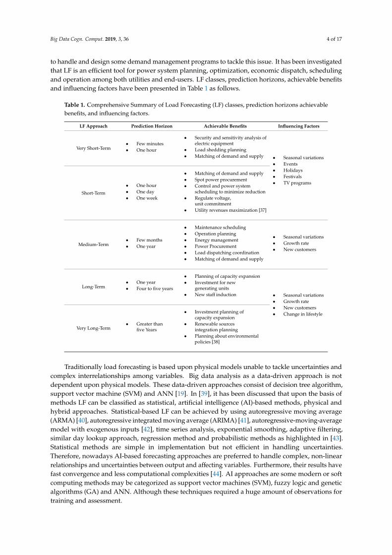
to handle and design some demand management programs to tackle this issue. It has been investigatedthat LF is an efficient tool for power system planning, optimization, economic dispatch, schedulingand operation among both utilities and end-users. LF classes, prediction horizons, achievable benefitsand influencing factors have been presented in Table 1 as follows.

Table 1. Comprehensive Summary of Load Forecasting (LF) classes, prediction horizons achievablebenefits, and influencing factors.

LF Approach Prediction Horizon Achievable Benefits Influencing Factors

Very Short-Term• Few minutes• One hour

• Security and sensitivity analysis ofelectric equipment

• Load shedding planning• Matching of demand and supply • Seasonal variations

• Events• Holidays• Festivals• TV programs

Short-Term

• One hour• One day• One week

• Matching of demand and supply• Spot power procurement• Control and power system

scheduling to minimize reduction• Regulate voltage,

unit commitment• Utility revenues maximization [37]

Medium-Term• Few months• One year

• Maintenance scheduling• Operation planning• Energy management• Power Procurement• Load dispatching coordination• Matching of demand and supply

• Seasonal variations• Growth rate• New customers

Long-Term• One year• Four to five years

• Planning of capacity expansion• Investment for new

generating units• New staff induction • Seasonal variations

• Growth rate• New customers• Change in lifestyle

Very Long-Term• Greater than

five Years

• Investment planning ofcapacity expansion

• Renewable sourcesintegration planning

• Planning about environmentalpolicies [38]

Traditionally load forecasting is based upon physical models unable to tackle uncertainties andcomplex interrelationships among variables. Big data analysis as a data-driven approach is notdependent upon physical models. These data-driven approaches consist of decision tree algorithm,support vector machine (SVM) and ANN [19]. In [39], it has been discussed that upon the basis ofmethods LF can be classified as statistical, artificial intelligence (AI)-based methods, physical andhybrid approaches. Statistical-based LF can be achieved by using autoregressive moving average(ARMA) [40], autoregressive integrated moving average (ARIMA) [41], autoregressive-moving-averagemodel with exogenous inputs [42], time series analysis, exponential smoothing, adaptive filtering,similar day lookup approach, regression method and probabilistic methods as highlighted in [43].Statistical methods are simple in implementation but not efficient in handling uncertainties.Therefore, nowadays AI-based forecasting approaches are preferred to handle complex, non-linearrelationships and uncertainties between output and affecting variables. Furthermore, their results havefast convergence and less computational complexities [44]. AI approaches are some modern or softcomputing methods may be categorized as support vector machines (SVM), fuzzy logic and geneticalgorithms (GA) and ANN. Although these techniques required a huge amount of observations fortraining and assessment.

Big Data Cogn. Comput. 2019, 3, 36 5 of 17

Unlike the statistical and AI-based forecasting approaches, the physical methods require detailedinformation for future prediction. Normally satellite is applied for short-term forecasting as exploredin [45]. For long-term forecasting weather-based numerical prediction models are appropriate.In addition to physical forecasting tools, hybrid methods combine different approaches to handlechallenges in standalone techniques. Several hybrid techniques comprise fuzzy neural network,fuzzy expert neural network system, neural expert systems and neural-genetic algorithm [46].Forecast studies have been mainly focused on aggregate loads but individual residential householdlevel and appliance level energy forecasts have not been analyzed [47]. With the recent advancementof smart grid, there is a growing interest for residential electricity analysis at individual household andappliance level for DR manipulation and optimum power system planning and operation Residentialload profiles show high uncertainty and variations in comparison to commercial or larger loads. This ismostly due to random residents’ behavior [48]. Hence, it is a greater challenge to forecast residentialloads at individual and appliance level.

In LF, past observations have been utilized to observe different variables relationship.Numerous short time horizon load prediction approaches have been explored in literature. Regression iscommonly applied in case of historic data unavailability. ANNs are preferred in case of uncertaintiesthat are difficult to manage by conventional tools. Indonesian South Sulawesi Island’s load has beenpredicted by regression based LF [49]. A short-term LF model was presented in [50] by applyingclustering regression. A fuzzy logic-based approach was applied for short time horizon load predictionwhich utilizes fuzzy rules that were obtained from past weather and load. In addition to this fuzzylogic, genetic and evolutionary algorithm were applied with ANN was also investigated in [46]. In [51],an online support vector regression algorithm was presented to forecast Surrey, British Columbiaresidential sector. In this paper there is investigation of AC load prediction by making use of multiplelinear regression, SCG and LMA-based ANN approach described as below.

4. LMA-based ANN Approach

ANN models have been applied for best execution through several small interrelated unitstermed as neurons. In order to achieve better results, simultaneous massive processing’s havebeen performed by neurons that have an artificial interconnection. Numerous repetitive processingis performed by neurons that also connect input, output and hidden layers of neural network.Relationship between input and output can be mapped by neurons weights updating that is achievedby training algorithm applied in ANN. Activation function generates output by making use of weightedinputs summation. Desired and generated output error can be minimized by adjustment of weightsand biases. Generally, neural network has been discussed in [52] can be represented mathematically in(1) as follows.

An =k∑

n=1

Pnwn (1)

where n = 1, 2, 3, ..., k, Pn is the nth input, wn is the allocated weight for nth input and An is thenth ANN output. ANN approaches have been reviewed in detail in [20]. For ANN calibrationnetwork architecture is selected and number of neurons will be selected as required. In addition,ANN training algorithm for weights updating will be decided. Speed, accuracy and complexity of loadforecasting model depends upon machine learning algorithm applied for model training. In this paper,a feed forward three-layer multi perceptron neural network has been proposed. By making use of anactivation function desired outcomes will be obtained by hidden neurons. Most commonly log-sigmoidmathematical function is applied for training. Transfer function for this proposed function [52] isrepresented as

F(n) =1

1 + e−n (2)

Big Data Cogn. Comput. 2019, 3, 36 6 of 17

In the proposed forecasting model, the LMA has been used to for hidden layer weights updating inorder to solve nonlinear least square problems. Various algorithms applied for multi-layer perceptionANN model training are LMA, gradient decent and Bayesian regularization. In the proposed forecastingapproach, the LMA has been used for weights updating of hidden layers in order achieve desiredoutcomes. In LMA, initially random weights wn are generated. Then sum square error En will becomputed from initial weights by using

En =12

∑1 ≤ p ≤ P1 ≤ o ≤ O

e2p,o (3)

where ep,o is training error that can be calculated from desired output dp,o and actual output Ap,o asgiven by

ep,o = dp,o −Ap,o (4)

After this LMA weights are updated by

wn+1 = wn − (H)−1 JEn (5)

where J is Jacobian matrix and H is hessian matrix that can be computed by

H = JT J + (βI) (6)

where I is unity matrix and β is combination coefficient that value will be considered if updatederror En+1 becomes less than original En. If updated error En+1 becomes greater than original En,then procedure will be again started from initial random weights generation [53–55]. LMA procedurecan be observed in detail from the following flow diagram given in Figure 1.

Big Data Cogn. Comput. 2019, 3, 36 7 of 17

Big Data Cogn. Comput. 2019, 3, x FOR PEER REVIEW 6 of 16

퐸 =12

푒 , (3)

where ep,o is training error that can be calculated from desired output dp,o and actual output Ap,o as given by

푒 , = 푑 , - 퐴 , (4)

After this LMA weights are updated by

푤 = 푤 - (퐻) 퐽퐸 (5)

where J is Jacobian matrix and H is hessian matrix that can be computed by

H= 퐽 J+ (β퐼) (6)

where I is unity matrix and β is combination coefficient that value will be considered if updated error En+1 becomes less than original En. If updated error En+1 becomes greater than original En, then procedure will be again started from initial random weights generation [53–55]. LMA procedure can be observed in detail from the following flow diagram given in Figure 1.

Figure 1. Flow chart for Levenberg–Marquardt Algorithm (LMA) considered in Artificial Neural

Network (ANN).

5. Performance Assessment Indices

To access the fitness of LF approaches, different performance evaluation indices have been applied. Firstly, the percentage absolute error has been computed to observe accuracy of proposed approach as given in Equation (7). Xi represents actual AC load, Yi represents AC load predictions by applied LF approach.

%퐴퐸 = x 100% (7)

Figure 1. Flow chart for Levenberg–Marquardt Algorithm (LMA) considered in Artificial NeuralNetwork (ANN).

5. Performance Assessment Indices

To access the fitness of LF approaches, different performance evaluation indices have been applied.Firstly, the percentage absolute error has been computed to observe accuracy of proposed approachas given in Equation (7). Xi represents actual AC load, Yi represents AC load predictions by appliedLF approach.

%AE =

∣∣∣∣∣Xi −YiXi

∣∣∣∣∣× 100% (7)

Secondly, the mean squared error MSE a performance assessment indicator, has been appliedto observe the applied LF approach accuracy for AC load predictions. Equation (8) shows how toformulate mean squared error. Ei is difference between observed and actual load for N observations.An MSE value closer to zero represents that the predicted outcome is more accurate.

MSE =1N

N∑i=1

(Ei)2 =

1N

N∑i=1

(Xi −Yi)2 (8)

Thirdly, the mean absolute percentage error (MAPE) that is also a performance assessmentindicator, to observe the applied LF approach accuracy for AC load predictions [56]. Equation (9)represents MAPE formulation as follows:

MAPE =1N

N∑i=1

∣∣∣∣∣Yi −XiYi

∣∣∣∣∣× 100% (9)

However, the greater variations in energy consumptions have been observed for smallerhouseholds. MSE and MAPE are not suitable accuracy predictions indicators in this case as powerconsumption varies greatly during peak and off-peak periods. Therefore, another performance

Big Data Cogn. Comput. 2019, 3, 36 8 of 17

indicator namely the mean absolute error (MAE) has been adopted to access accuracy of appliedapproach for AC load predictions that can be formulated as,

MAE =

∑Ni=1 (Yi −Xi)

N(10)

The whole procedure adopted for LMA-based ANN including performance assessment indices isgiven in the following flow chart given in Figure 2.

Big Data Cogn. Comput. 2019, 3, x FOR PEER REVIEW 7 of 16

Secondly, the mean squared error MSE a performance assessment indicator, has been applied to observe the applied LF approach accuracy for AC load predictions. Equation (8) shows how to formulate mean squared error. Ei is difference between observed and actual load for N observations. An MSE value closer to zero represents that the predicted outcome is more accurate.

푀푆퐸 =1푁

( 퐸 ) =1푁

( 푋 − 푌 ) (8)

Thirdly, the mean absolute percentage error (MAPE) that is also a performance assessment indicator, to observe the applied LF approach accuracy for AC load predictions [56]. Equation (9) represents MAPE formulation as follows:

푀퐴푃퐸 = ∑ x 100% (9)

However, the greater variations in energy consumptions have been observed for smaller households. MSE and MAPE are not suitable accuracy predictions indicators in this case as power consumption varies greatly during peak and off-peak periods. Therefore, another performance indicator namely the mean absolute error (MAE) has been adopted to access accuracy of applied approach for AC load predictions that can be formulated as,

푀퐴퐸 =∑ (푌 − 푋 )

푁 (10)

The whole procedure adopted for LMA-based ANN including performance assessment indices is given in the following flow chart given in Figure 2.

Figure 2. Flow chart for LMA-based ANN.

6. Case Studies

The residential AC real time hourly TMY3 data for Austin Texas are served for demonstrating the effectiveness of the proposed LMA-based ANN AC load forecasting approach. TMY3 represents typical metrological yearly parameters of different locations. Data collected is most accurate and recommended to forecast buildings energy consumption. It represents typical data for 1020 different regions that has been utilized nowadays, an improved version as compared to old version TMY2 and initial TMY collected information [57,58]. All forecast results have been obtained by making use of Statistics and Machine Learning and Neural Network Toolboxes in MATLAB R2016b. Accuracy of

Figure 2. Flow chart for LMA-based ANN.

6. Case Studies

The residential AC real time hourly TMY3 data for Austin Texas are served for demonstratingthe effectiveness of the proposed LMA-based ANN AC load forecasting approach. TMY3 representstypical metrological yearly parameters of different locations. Data collected is most accurate andrecommended to forecast buildings energy consumption. It represents typical data for 1020 differentregions that has been utilized nowadays, an improved version as compared to old version TMY2 andinitial TMY collected information [57,58]. All forecast results have been obtained by making use ofStatistics and Machine Learning and Neural Network Toolboxes in MATLAB R2016b. Accuracy offorecasting approach is affected due to numerous parameters. Figure 2. presents the input variablesapplied for AC load predictions. Overall accuracy and efficiency of proposed LF approach have beenaccessed by input variables data like time, weather and load. Large number and volume of input datais used to analyze forecasting results. AC load variations profile during complete year 2014 for AustinTexas that has been applied also as an input can be observed from the Figure 3 given below.

Big Data Cogn. Comput. 2019, 3, 36 9 of 17

Big Data Cogn. Comput. 2019, 3, x FOR PEER REVIEW 8 of 16

forecasting approach is affected due to numerous parameters. Figure 2. presents the input variables applied for AC load predictions. Overall accuracy and efficiency of proposed LF approach have been accessed by input variables data like time, weather and load. Large number and volume of input data is used to analyze forecasting results. AC load variations profile during complete year 2014 for Austin Texas that has been applied also as an input can be observed from the Figure 3 given below.

Figure 3. Air Conditioner (AC) Load variations during complete year.

Number of input variables have been applied to predict AC load. Some relationships are mentioned here to show the big data involvement in power systems nowadays. Huge amount of data is applied to check accuracy of LMA-based ANN approach. In other words, big data analysis has been performed for AC load prediction. Meanwhile, the effect of Dew Point and Dry Bulb temperature over AC loads can be visualized from Figure 4.

(a)

AC lo

ad (W

atts

)

Dew

Poi

nt (C

entig

rade

)

Figure 3. Air Conditioner (AC) Load variations during complete year.

Number of input variables have been applied to predict AC load. Some relationships arementioned here to show the big data involvement in power systems nowadays. Huge amount of datais applied to check accuracy of LMA-based ANN approach. In other words, big data analysis has beenperformed for AC load prediction. Meanwhile, the effect of Dew Point and Dry Bulb temperature overAC loads can be visualized from Figure 4.

Big Data Cogn. Comput. 2019, 3, x FOR PEER REVIEW 8 of 16

forecasting approach is affected due to numerous parameters. Figure 2. presents the input variables applied for AC load predictions. Overall accuracy and efficiency of proposed LF approach have been accessed by input variables data like time, weather and load. Large number and volume of input data is used to analyze forecasting results. AC load variations profile during complete year 2014 for Austin Texas that has been applied also as an input can be observed from the Figure 3 given below.

Figure 3. Air Conditioner (AC) Load variations during complete year.

Number of input variables have been applied to predict AC load. Some relationships are mentioned here to show the big data involvement in power systems nowadays. Huge amount of data is applied to check accuracy of LMA-based ANN approach. In other words, big data analysis has been performed for AC load prediction. Meanwhile, the effect of Dew Point and Dry Bulb temperature over AC loads can be visualized from Figure 4.

(a)

AC lo

ad (W

atts

)

Dew

Poi

nt (C

entig

rade

)

Big Data Cogn. Comput. 2019, 3, x FOR PEER REVIEW 9 of 16

(b)

Figure 4. AC Load variations due to (a) Dew Point Temperature (b) Dry Bulb Temperature.

Both statistical and ANN based models have been validated for residential AC real time hourly TMY3 data for Austin Texas. The actual and forecasted residential AC load by applying conventional statistical multiple linear regression approach can be observed in Figure 5.

Figure 5. Actual and forecasted AC loads by multiple linear regression approach.

Furthermore, both actual and forecasted residential AC loads by applying SCG-based ANN can be observed in Figure 6. For ANN architecture, eight variables have been applied as input. Each input variable comprises yearly observations as input. The number of neurons is set to 10 with sigmoid transfer function in hidden layer. A single output will be achieved that represent predicted AC load. This method makes use of about 70% input data for training and 15% input data for testing and 15% of input data for validation of SCG-based ANN.

Dry

Bul

b (C

entig

rade

)

AC

Loa

d (W

atts

)

Figure 4. AC Load variations due to (a) Dew Point Temperature (b) Dry Bulb Temperature.

Big Data Cogn. Comput. 2019, 3, 36 10 of 17

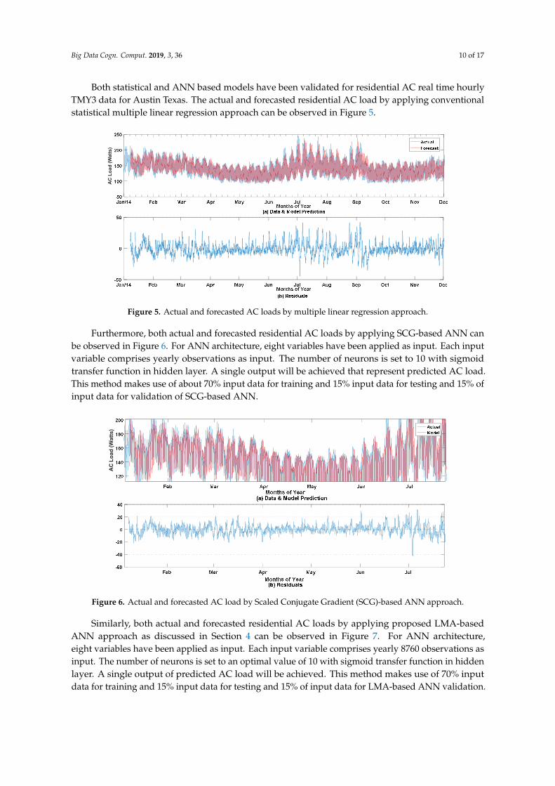
Both statistical and ANN based models have been validated for residential AC real time hourlyTMY3 data for Austin Texas. The actual and forecasted residential AC load by applying conventionalstatistical multiple linear regression approach can be observed in Figure 5.

Big Data Cogn. Comput. 2019, 3, x FOR PEER REVIEW 9 of 16

(b)

Figure 4. AC Load variations due to (a) Dew Point Temperature (b) Dry Bulb Temperature.

Both statistical and ANN based models have been validated for residential AC real time hourly TMY3 data for Austin Texas. The actual and forecasted residential AC load by applying conventional statistical multiple linear regression approach can be observed in Figure 5.

Figure 5. Actual and forecasted AC loads by multiple linear regression approach.

Furthermore, both actual and forecasted residential AC loads by applying SCG-based ANN can be observed in Figure 6. For ANN architecture, eight variables have been applied as input. Each input variable comprises yearly observations as input. The number of neurons is set to 10 with sigmoid transfer function in hidden layer. A single output will be achieved that represent predicted AC load. This method makes use of about 70% input data for training and 15% input data for testing and 15% of input data for validation of SCG-based ANN.

Dry

Bul

b (C

entig

rade

)

AC

Loa

d (W

atts

)

Figure 5. Actual and forecasted AC loads by multiple linear regression approach.

Furthermore, both actual and forecasted residential AC loads by applying SCG-based ANN canbe observed in Figure 6. For ANN architecture, eight variables have been applied as input. Each inputvariable comprises yearly observations as input. The number of neurons is set to 10 with sigmoidtransfer function in hidden layer. A single output will be achieved that represent predicted AC load.This method makes use of about 70% input data for training and 15% input data for testing and 15% ofinput data for validation of SCG-based ANN.Big Data Cogn. Comput. 2019, 3, x FOR PEER REVIEW 10 of 16

Figure 6. Actual and forecasted AC load by Scaled Conjugate Gradient (SCG)-based ANN approach.

Similarly, both actual and forecasted residential AC loads by applying proposed LMA-based ANN approach as discussed in Section 4 can be observed in Figure 7. For ANN architecture, eight variables have been applied as input. Each input variable comprises yearly 8760 observations as input. The number of neurons is set to an optimal value of 10 with sigmoid transfer function in hidden layer. A single output of predicted AC load will be achieved. This method makes use of 70% input data for training and 15% input data for testing and 15% of input data for LMA-based ANN validation.

Figure 7. Actual and forecasted AC load by LMA-based ANN approach.

The performance comparisons of multiple linear regression, SCG and LMA-based ANN approach for AC load forecast by making use of performance assessment indices as discussed in section 5 shown in Table 2.

Table 2. Comparisons of performance assessment indices for multiple linear regression SCG and LMA-based ANN approach.

Multiple Linear Regression SCG-based ANN LMA-based ANN Hour Actual Predicted %AE Predicted %AE Predicted %AE

1 129.60 144.31 5.26 131.49 1.46 136.41 5.26 2 124.27 141.02 5.65 131.29 5.65 131.29 5.65

AC L

oad

(Wat

ts)

AC L

oad

(Wat

ts)

Figure 6. Actual and forecasted AC load by Scaled Conjugate Gradient (SCG)-based ANN approach.

Similarly, both actual and forecasted residential AC loads by applying proposed LMA-basedANN approach as discussed in Section 4 can be observed in Figure 7. For ANN architecture,eight variables have been applied as input. Each input variable comprises yearly 8760 observations asinput. The number of neurons is set to an optimal value of 10 with sigmoid transfer function in hiddenlayer. A single output of predicted AC load will be achieved. This method makes use of 70% inputdata for training and 15% input data for testing and 15% of input data for LMA-based ANN validation.

Big Data Cogn. Comput. 2019, 3, 36 11 of 17

Figure 7. Actual and forecasted AC load by LMA based ANN approach.

May Jun Jul Aug Sep Oct Nov Dec

Months of Year

50

100

150

200

250AC

Loa

d (W

atts

)

(a) Data & Model Prediction

ActualForecast

May Jun Jul Aug Sep Oct Nov DecMonths of Year

-40

-20

0

20

40

(b) Residuals

Figure 7. Actual and forecasted AC load by LMA-based ANN approach.

The performance comparisons of multiple linear regression, SCG and LMA-based ANN approachfor AC load forecast by making use of performance assessment indices as discussed in Section 5 shownin Table 2.

Table 2. Comparisons of performance assessment indices for multiple linear regression SCG andLMA-based ANN approach.

Multiple LinearRegression SCG-Based ANN LMA-Based ANN

Hour Actual Predicted %AE Predicted %AE Predicted %AE

1 129.60 144.31 5.26 131.49 1.46 136.41 5.262 124.27 141.02 5.65 131.29 5.65 131.29 5.653 120.89 139.27 6.12 131.78 9.01 128.29 6.124 119.48 139.07 7.13 133.15 11.44 128.00 7.135 119.96 141.09 8.98 135.88 13.27 130.73 8.986 123.18 147.60 11.51 141.03 14.49 137.35 11.517 129.91 159.20 13.14 148.64 14.42 146.98 13.148 138.11 166.99 10.66 154.49 11.86 152.84 10.669 147.38 170.49 5.74 158.07 7.25 155.85 5.7410 155.07 172.81 1.25 160.52 3.52 157.01 1.2511 159.14 173.72 1.54 161.90 1.73 156.69 1.5412 160.29 172.65 2.66 162.31 1.26 156.02 2.6613 159.40 170.55 2.62 162.10 1.69 155.23 2.6214 157.09 168.46 1.39 161.77 2.98 154.90 1.3915 154.99 165.95 0.28 161.18 3.99 155.43 0.2816 155.96 165.71 1.54 161.07 3.27 158.36 1.5417 162.86 172.54 1.09 163.30 0.27 164.64 1.0918 167.66 180.35 0.07 165.67 1.19 167.78 0.0719 164.53 178.28 1.89 164.33 0.12 167.64 1.8920 158.47 173.62 3.92 162.05 2.26 164.68 3.9221 152.15 168.57 4.23 159.26 4.67 158.59 4.2322 143.47 161.65 4.97 154.34 7.58 150.60 4.9723 134.31 152.91 5.01 147.31 9.68 141.04 5.0124 124.61 143.29 4.73 138.69 11.30 130.50 4.73

Maximum 180.35 22.54 165.67 14.49 167.78 13.14

MSE % 9.68 8.30 5.57

MAPE % 4.9529 4.2782 2.9221

MAE(Wh) 7.2294 6.2456 4.2371

DailyMAPE % 4.3743 4.1249 2.5348

The MSE and MAPE are performance assessment indicators that have been formulated by (7) and(8) respectively. Difference between desired and actual output can be shown by error performance

Big Data Cogn. Comput. 2019, 3, 36 12 of 17

output from these indicators. LMA-based ANN for AC demand LF is showing error performance of94.43% and 97.00% by MSE and MAPE respectively that is bitter higher than SCG-based ANN andstatistical multiple linear regression-based approach.

Furthermore, MAE can be computed from (9) that represents mean absolute error.Figure 8 represents error distribution for LMA-based ANN approach. Most samples are in thepositive region, which shows better results. Also, MAE can be observed from red line in error histogramthat is about 4.2371Wh. In addition to this MAPE can be observed for LMA-based ANN approachthat is approximately about 2.9221% as indicated by red line. It has been observed that in additionto error performance improvement LMA-based ANN has highest computation speed in contrast toSCG-based ANN for big data analysis. Performance indices values indicate more accurate value forproposed LMA-based ANN as observed from Table 2. It can be applied to predict appliance levelloads like AC with more accuracy as compared to SCG-based ANN and conventional multiple linearregression-based approach.

Big Data Cogn. Comput. 2019, 3, x FOR PEER REVIEW 11 of 16

3 120.89 139.27 6.12 131.78 9.01 128.29 6.12 4 119.48 139.07 7.13 133.15 11.44 128.00 7.13 5 119.96 141.09 8.98 135.88 13.27 130.73 8.98 6 123.18 147.60 11.51 141.03 14.49 137.35 11.51 7 129.91 159.20 13.14 148.64 14.42 146.98 13.14 8 138.11 166.99 10.66 154.49 11.86 152.84 10.66 9 147.38 170.49 5.74 158.07 7.25 155.85 5.74 10 155.07 172.81 1.25 160.52 3.52 157.01 1.25 11 159.14 173.72 1.54 161.90 1.73 156.69 1.54 12 160.29 172.65 2.66 162.31 1.26 156.02 2.66 13 159.40 170.55 2.62 162.10 1.69 155.23 2.62 14 157.09 168.46 1.39 161.77 2.98 154.90 1.39 15 154.99 165.95 0.28 161.18 3.99 155.43 0.28 16 155.96 165.71 1.54 161.07 3.27 158.36 1.54 17 162.86 172.54 1.09 163.30 0.27 164.64 1.09 18 167.66 180.35 0.07 165.67 1.19 167.78 0.07 19 164.53 178.28 1.89 164.33 0.12 167.64 1.89 20 158.47 173.62 3.92 162.05 2.26 164.68 3.92 21 152.15 168.57 4.23 159.26 4.67 158.59 4.23 22 143.47 161.65 4.97 154.34 7.58 150.60 4.97 23 134.31 152.91 5.01 147.31 9.68 141.04 5.01 24 124.61 143.29 4.73 138.69 11.30 130.50 4.73

Maximum 180.35 22.54 165.67 14.49 167.78 13.14 MSE % 9.68 8.30 5.57

MAPE % 4.9529 4.2782 2.9221 MAE(Wh) 7.2294 6.2456 4.2371

Daily MAPE %

4.3743 4.1249 2.5348

The MSE and MAPE are performance assessment indicators that have been formulated by (7) and (8) respectively. Difference between desired and actual output can be shown by error performance output from these indicators. LMA-based ANN for AC demand LF is showing error performance of 94.43% and 97.00% by MSE and MAPE respectively that is bitter higher than SCG-based ANN and statistical multiple linear regression-based approach.

Figure 8. Error distribution histogram.

Furthermore, MAE can be computed from (9) that represents mean absolute error. Figure 8 represents error distribution for LMA-based ANN approach. Most samples are in the positive region, which shows better results. Also, MAE can be observed from red line in error histogram that is about 4.2371Wh. In addition to this MAPE can be observed for LMA-based ANN approach that is

AC

Loa

d (W

atts

)A

C L

oad

(Wat

ts)

AC

Loa

d (W

atts

)

Figure 8. Error distribution histogram.

Furthermore, AC load prediction by utilizing LMA-based ANN approach for some weeks can beshown in Figure 9. It can be depicted that load predictions shows little difference from the actual one.Also, MAPE gives a less error value of 6.16% for selected weeks with prediction performance accuracyof 93.84%.

Big Data Cogn. Comput. 2019, 3, x FOR PEER REVIEW 12 of 16

approximately about 2.9221% as indicated by red line. It has been observed that in addition to error performance improvement LMA-based ANN has highest computation speed in contrast to SCG-based ANN for big data analysis. Performance indices values indicate more accurate value for proposed LMA-based ANN as observed from Table 2. It can be applied to predict appliance level loads like AC with more accuracy as compared to SCG-based ANN and conventional multiple linear regression-based approach.

Furthermore, AC load prediction by utilizing LMA-based ANN approach for some weeks can be shown in Figure 9. It can be depicted that load predictions shows little difference from the actual one. Also, MAPE gives a less error value of 6.16% for selected weeks with prediction performance accuracy of 93.84%.

Figure 9. Comparison of forecast and actual load for every week.

In addition, it is possible to obtain AC load forecast results for different time horizons like hourly, weekly and monthly basis by making use of LMA-based ANN approach more accurately. Breakdown of error statistics by using LMA-based ANN approach for AC load predictions can be observed visually on hourly, weekly and monthly basis by each box in Figure 10. It can be seen from Figure 10 that that median forecast percent is almost zero as observed from central line of boxes in boxplots at different hours, days and months of year. The maximum value of forecast percent error is less than about 5% during different time horizons. The bottom line of the boxes indicates that 25% of AC load predicted values have about zero percent error while from top line of boxes it can be extracted that 75% of AC load predicted values have percent error of about less than 5%. From boxplot observations, it can also be visualized that due to increase in time span to predict load more values falls out of range showed using +. Furthermore, interquartile range of percent error of AC predicted loads can be observed from difference between top and bottom of boxes in box plots that presents accurate and considerable value of about less than 5% by making use of LMA-based ANN.

AC

Loa

d (W

atts

)

Figure 9. Comparison of forecast and actual load for every week.

Big Data Cogn. Comput. 2019, 3, 36 13 of 17

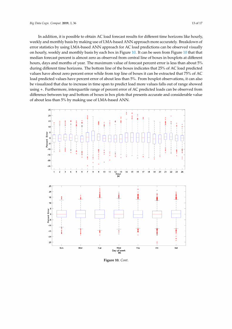
In addition, it is possible to obtain AC load forecast results for different time horizons like hourly,weekly and monthly basis by making use of LMA-based ANN approach more accurately. Breakdown oferror statistics by using LMA-based ANN approach for AC load predictions can be observed visuallyon hourly, weekly and monthly basis by each box in Figure 10. It can be seen from Figure 10 that thatmedian forecast percent is almost zero as observed from central line of boxes in boxplots at differenthours, days and months of year. The maximum value of forecast percent error is less than about 5%during different time horizons. The bottom line of the boxes indicates that 25% of AC load predictedvalues have about zero percent error while from top line of boxes it can be extracted that 75% of ACload predicted values have percent error of about less than 5%. From boxplot observations, it can alsobe visualized that due to increase in time span to predict load more values falls out of range showedusing +. Furthermore, interquartile range of percent error of AC predicted loads can be observed fromdifference between top and bottom of boxes in box plots that presents accurate and considerable valueof about less than 5% by making use of LMA-based ANN.Big Data Cogn. Comput. 2019, 3, x FOR PEER REVIEW 13 of 16

Figure 10. Breakdown of error statistics for load predictions (a) hourly, (b) weekly and (c) monthly.

7. Conclusions

In this paper, it has been investigated that AC impact in overall electricity consumption in buildings is very high. Therefore, controlling ACs power consumption is a significant factor for DR programs. Different evidence regarding AC load increase has been investigated worldwide. In addition to this, various big data analysis applications in power systems and load forecasting categories have been explored. Furthermore, this paper presents LMA-based ANN approach for residential AC load forecasting. Different performance assessment indices have also been

Perc

ent

Err

orPe

rcen

t Er

ror

Perc

ent

Erro

r

Figure 10. Cont.

Big Data Cogn. Comput. 2019, 3, 36 14 of 17

Perc

ent

Erro

r

Figure 10. Breakdown of error statistics for load predictions (a) hourly, (b) weekly and (c) monthly.

7. Conclusions

In this paper, it has been investigated that AC impact in overall electricity consumption inbuildings is very high. Therefore, controlling ACs power consumption is a significant factor forDR programs. Different evidence regarding AC load increase has been investigated worldwide.In addition to this, various big data analysis applications in power systems and load forecastingcategories have been explored. Furthermore, this paper presents LMA-based ANN approach forresidential AC load forecasting. Different performance assessment indices have also been investigated.Error formulations have shown that LMA-based ANN approach for residential AC load forecastingpresents better results in comparison to SCG-based ANN and conventional multiple linear regressionapproach. It has been observed that, in addition to error performance improvement, LMA-based ANNhas the highest computation speed in contrast to SCG-based ANN for big sets of input data samples.Furthermore, information of AC load is obtainable for different time horizons like weekly, hourly,and monthly bases most accurately due to better LMA-based ANN prediction accuracy. It can beapplied to predict appliance level loads like AC with more accuracy as compared to SCG-based ANNand conventional regression-based approaches.

Author Contributions: M.W. and Z.L. conceptualized the study; M.W. performed the analyses; Z.L. and L.Y.acquired funding; Z.L., M.W. performed investigations; L.Y., M.W. and Z.L. acquired resources; M.W. wrote theoriginal draft; and M.W., Z.L. and L.Y. reviewed and edited the manuscript.

Funding: This work was supported by the National Key R&D Program of China under Grant 2016YFB0901100and the Fundamental Research Funds for the Central Universities under Grant 2019QNA4023.

Conflicts of Interest: The authors declare no conflict of interest.

References

1. Garcia-Valle, R.; Silva, L.C.P.D.; Xu, Z.; Ostergaard, J.J. Smart demand for improving short-term voltagecontrol on distribution networks. IET Gener. Transm. Distrib. 2009, 3, 724–732. [CrossRef]

2. Paridari, K.; Nordstrom, L.; Sandels, C. Aggregator strategy for planning demand response resources underuncertainty based on load flexibility modeling. In Proceedings of the 2017 IEEE International Conference onSmart Grid Communications (SmartGridComm), Dresden, Germany, 23–27 October 2017; pp. 338–343.

3. De Cian, E.; Wing, I.S. Global energy consumption in a warming climate. Environ. Resour. Econ. 2019, 72, 365–410.[CrossRef]

4. Santamouris, M.; Sfakianaki, A.; Pavlou, K. On the efficiency of night ventilation techniques applied toresidential buildings. Energy Build. 2010, 42, 1309–1313. [CrossRef]

5. Ahmad, M.I.; Jarimi, H.; Riffat, S. Introduction: Overview of Buildings and Passive Cooling Technique.In Nocturnal Cooling Technology for Building Applications; Springer: Berlin, Germany, 2019; pp. 1–6.

6. Malik, A.; Haghdadi, N.; MacGill, I.; Ravishankar, J. Appliance level data analysis of summer demandreduction potential from residential air conditioner control. Appl. Energy 2019, 235, 776–785. [CrossRef]

Big Data Cogn. Comput. 2019, 3, 36 15 of 17

7. Borlase, S. Smart Grids: Infrastructure, Technology, and Solutions; CRC Press: Boca Raton, FL, USA, 2016.8. Conti, J.; Holtberg, P.; Diefenderfer, J.; LaRose, A.; Turnure, J.T.; Westfall, L. International Energy Outlook 2016

with Projections to 2040; USDOE Energy Information Administration (EIA): Washington, DC, USA, 2016.9. Haider, H.T.; See, O.H.; Elmenreich, W. A review of residential demand response of smart grid. Renew. Sustain.

Energy Rev. 2016, 59, 166–178. [CrossRef]10. Shao, C.; Ding, Y.; Siano, P.; Lin, Z. A framework for incorporating demand response of smart buildings into

the integrated heat and electricity energy system. IEEE Trans. Ind. Electron. 2019, 66, 1465–1475. [CrossRef]11. Siano, P.; Sarno, D. Assessing the benefits of residential demand response in a real time distribution energy

market. Appl. Energy 2016, 161, 533–551. [CrossRef]12. Swan, L.G.; Ugursal, V.I. Modeling of end-use energy consumption in the residential sector: A review of

modeling techniques. Renew. Sustain. Energy Rev. 2009, 13, 1819–1835. [CrossRef]13. Bourdeau, M.; Zhai, X.-Q.; Nefzaoui, E.; Guo, X.; Chatellier, P. Modelling and forecasting building energy

consumption: A review of data-driven techniques. Sustain. Cities Soc. 2019. [CrossRef]14. Cai, H.; Shen, S.; Lin, Q.; Li, X.; Xiao, H. Predicting the energy consumption of residential buildings for

regional electricity supply-side and demand-side management. IEEE Access 2019, 7, 30386–30397. [CrossRef]15. Zhou, B.; Li, W.; Chan, K.W.; Cao, Y.; Kuang, Y.; Liu, X.; Wang, X. Smart home energy management systems:

Concept, configurations, and scheduling strategies. Renew. Sustain. Energy Rev. 2016, 61, 30–40. [CrossRef]16. Hu, M.; Xiao, F. Price-responsive model-based optimal demand response control of inverter air conditioners

using genetic algorithm. Appl. Energy 2018, 219, 151–164. [CrossRef]17. Chen, M.; Mao, S.; Liu, Y. Big data: A survey. Mob. Netw. Appl. 2014, 19, 171–209. [CrossRef]18. Soliman, S.A.; Al-Kandari, A.M. Electrical Load Forecasting: Modeling and Model Construction; Elsevier:

Amsterdam, The Netherlands, 2010.19. Ye, C.J.; Ding, Y.; Wang, P.; Lin, Z. A Data-driven Bottom-up Approach for Spatial and Temporal Electric

Load Forecasting. IEEE Trans. Power Syst. 2019, 34, 1966–1979. [CrossRef]20. Koseleva, N.; Ropaite, G. Big data in building energy efficiency: Understanding of big data and main

challenges. Procedia Eng. 2017, 172, 544–549. [CrossRef]21. Khan, A.R.; Razzaq, S.; Alquthami, T.; Moghal, M.R.; Amin, A.; Mahmood, A. Day ahead load forecasting for IESCO

using Artificial Neural Network and Bagged Regression Tree. In Proceedings of the 2018 1st International Conferenceon Power, Energy and Smart Grid (ICPESG), Mirpur, Pakistan, 12–13 April 2018; pp. 1–6.

22. Osman, A.M.S. A novel big data analytics framework for smart cities. Future Gener. Comput. Syst. 2019, 91, 620–633.[CrossRef]

23. Elgendy, N.; Elragal, A. Big data analytics: A literature review paper. In Proceedings of the IndustrialConference on Data Mining, St. Petersburg, Russia, 16–20 July 2014; pp. 214–227.

24. Shim, J.P.; French, A.M.; Guo, C.; Jablonski, J. Big Data and Analytics: Issues, Solutions, and ROI. CAIS2015, 37, 39. [CrossRef]

25. Akhavan-Hejazi, H.; Mohsenian-Rad, H. Power systems big data analytics: An assessment of paradigm shiftbarriers and prospects. Energy Rep. 2018, 4, 91–100. [CrossRef]

26. Yu, N.; Shah, S.; Johnson, R.; Sherick, R.; Hong, M.; Loparo, K. Big data analytics in power distributionsystems. In Proceedings of the 2015 IEEE Power & Energy Society Innovative Smart Grid TechnologiesConference (ISGT), Washington, DC, USA, 17–20 February 2015; pp. 1–5.

27. Zhang, D.; Qiu, R.C. Research on big data applications in Global Energy Interconnection.Glob. Energy Interconnect. 2018, 1, 352–357.

28. Grolinger, K.; L’Heureux, A.; Capretz, M.A.; Seewald, L. Energy forecasting for event venues: Big data andprediction accuracy. Energy Build. 2016, 112, 222–233. [CrossRef]

29. Hong, T. Big data analytics: Making the smart grid smarter. IEEE Power Energy Mag. 2018, 16, 12–16.[CrossRef]

30. Pérez-Chacón, R.; Luna-Romera, J.; Troncoso, A.; Martínez-Álvarez, F.; Riquelme, J. Big data analytics fordiscovering electricity consumption patterns in smart cities. Energies 2018, 11, 683. [CrossRef]

31. Wang, P.; Liu, B.; Hong, T. Electric load forecasting with recency effect: A big data approach. Int. J. Forecast.2016, 32, 585–597. [CrossRef]

32. Davis, L.W.; Gertler, P.J. Contribution of air conditioning adoption to future energy use under global warming.Proc. Natl. Acad. Sci. USA 2015, 112, 5962–5967. [CrossRef] [PubMed]

Big Data Cogn. Comput. 2019, 3, 36 16 of 17

33. Gungor, V.C.; Sahin, D.; Kocak, T.; Ergut, S.; Buccella, C.; Cecati, C.; Hancke, G.P. A survey on smart gridpotential applications and communication requirements. IEEE Trans. Ind. Inform. 2012, 9, 28–42. [CrossRef]

34. Sivak, M. Potential energy demand for cooling in the 50 largest metropolitan areas of the world: Implicationsfor developing countries. Energy Policy 2009, 37, 1382–1384. [CrossRef]

35. Santamouris, M. Cooling the buildings–past, present and future. Energy Build. 2016, 128, 617–638. [CrossRef]36. Kim, D.H.; Yoon, Y.T.; Lee, S.S.; Lee, S.K. Power system restoration plan using the characteristics of scale-free

networks. Eur. Trans. Electr. Power 2008, 18, 809–819. [CrossRef]37. Hong, T. Short-Term Electric Load Forecasting. Available online: https://www.researchgate.net/publication/

279683748_Short_Term_Electric_Load_Forecasting (accessed on 12 May 2019).38. Singh, A.K.; Khatoon, S.; Muazzam, M.; Chaturvedi, D. Load forecasting techniques and methodologies:

A review. In Proceedings of the 2012 2nd International Conference on Power, Control and EmbeddedSystems, Allahabad, India, 17–19 December 2012; pp. 1–10.

39. Campbell, S.D.; Diebold, F.X. Weather forecasting for weather derivatives. J. Am. Stat. Assoc. 2005, 100, 6–16.[CrossRef]

40. Xie, J.; Hong, T. Load forecasting using 24 solar terms. J. Mod. Power Syst. Clean Energy 2018, 6, 208–214.[CrossRef]

41. Pedro, H.T.; Coimbra, C.F. Assessment of forecasting techniques for solar power production with noexogenous inputs. Sol. Energy 2012, 86, 2017–2028. [CrossRef]

42. Li, Y.; Su, Y.; Shu, L. An ARMAX model for forecasting the power output of a grid connected photovoltaicsystem. Renew. Energy 2014, 66, 78–89. [CrossRef]

43. Bessa, R.J.; Trindade, A.; Silva, C.S.; Miranda, V. Probabilistic solar power forecasting in smart grids usingdistributed information. Int. J. Electr. Power Energy Syst. 2015, 72, 16–23. [CrossRef]

44. Raza, M.Q.; Khosravi, A. A review on artificial intelligence based load demand forecasting techniques forsmart grid and buildings. Renew. Sustain. Energy Rev. 2015, 50, 1352–1372. [CrossRef]

45. Abdel-Nasser, M.; Mahmoud, K. Accurate photovoltaic power forecasting models using deep LSTM-RNN.Neural Comput. Appl. 2017. [CrossRef]

46. Samuel, I.; Ojewola, T.; Awelewa, A.; Amaize, P. Short-Term Load Forecasting Using the Time Series andArtificial Neural Network Methods. J. Electr. Electron. Eng. 2016, 11, 72–81.

47. Kavgic, M.; Mavrogianni, A.; Mumovic, D.; Summerfield, A.; Stevanovic, Z.; Djurovic-Petrovic, M. A review ofbottom-up building stock models for energy consumption in the residential sector. Build. Environ. 2010, 45, 1683–1697.[CrossRef]

48. Rossi, M.; Brunelli, D. Electricity demand forecasting of single residential units. In Proceedings of the 2013 IEEEWorkshop on Environmental Energy and Structural Monitoring Systems, Trento, Italy, 11–12 September 2013;pp. 1–6.

49. Amral, N.; Ozveren, C.; King, D. Short-term load forecasting using multiple linear regression. In Proceedingsof the 2007 42th International Universities Power Engineering Conference (UPEC), Brighton, UK,4–6 September 2007; pp. 1192–1198.

50. Lei, J.; Jin, T.; Hao, J.; Li, F. Short-term load forecasting with clustering–regression model in distributedcluster. Clust. Comput. 2017. [CrossRef]

51. Dhillon, J.; Rahman, S.A.; Ahmad, S.U.; Hossain, M.J. Peak electricity load forecasting using online supportvector regression. In Proceedings of the 2016 IEEE Canadian Conference on Electrical and ComputerEngineering (CCECE), Vancouver, BC, Canada, 15–18 May 2016; pp. 1–4.

52. Hippert, H.S.; Pedreira, C.E.; Souza, R.C. Neural networks for short-term load forecasting: A review andevaluation. IEEE Trans. Power Syst. 2001, 16, 44–55. [CrossRef]

53. Du, Y.-C.; Stephanus, A. Levenberg–Marquardt Neural Network Algorithm for Degree of ArteriovenousFistula Stenosis Classification Using a Dual Optical Photoplethysmography Sensor. Sensors 2018, 18, 2322.[CrossRef]

54. Lv, C.; Xing, Y.; Zhang, J.; Na, X.; Li, Y.; Liu, T.; Cao, D.; Wang, F.-Y. Levenberg–Marquardt BackpropagationTraining of Multilayer Neural Networks for State Estimation of a Safety Critical Cyber-Physical System.IEEE Trans. Ind. Inform. 2017, 14, 3436–3446. [CrossRef]

55. Yu, H.; Wilamowski, B.; Yu, H.; Wilamowski, B.M. Levenberg Marquardt Training Industrial Electronics Handbook,Intelligent Systems, 2nd ed.; CRC Press: Boca Raton, FL, USA, 2011; Volume 12, pp. 12–15.

Big Data Cogn. Comput. 2019, 3, 36 17 of 17

56. Javed, F.; Arshad, N.; Wallin, F.; Vassileva, I.; Dahlquist, E. Forecasting for demand response in smartgrids: An analysis on use of anthropologic and structural data and short-term multiple loads forecasting.Appl. Energy 2012, 96, 150–160. [CrossRef]

57. National Renewable Energy Laboratory (NREL). Home Page. Available online: https://www.nrel.gov(accessed on 12 May 2019).

58. Wilcox, S.; Marion, W. Users Manual for Tmy3 Data Sets (Revised); National Renewable Energy Lab. (NREL):Golden, CO, USA, 2008.

© 2019 by the authors. Licensee MDPI, Basel, Switzerland. This article is an open accessarticle distributed under the terms and conditions of the Creative Commons Attribution(CC BY) license (http://creativecommons.org/licenses/by/4.0/).