Data-Driven Pedestrian Simulation Using Conditional Transition Maps AmandaBostr¨om Computer Science, Degree Project in Simulation and Development of Computer Games, Advanced Course, 15 Credits Program in Simulation and Computer Games Technology, 180 Credits ¨ Orebro, Sweden, Spring 2015 Examiner: Martin Magnusson Data-Driven Pedestrian Simulation Using Conditional Transition Maps
Transcript
Data-Driven PedestrianSimulation Using Conditional
Transition Maps
Amanda Bostrom
Computer Science, Degree Project in Simulation and Developmentof Computer Games, Advanced Course, 15 Credits
Program in Simulation and Computer Games Technology, 180 Credits
Orebro, Sweden, Spring 2015
Examiner: Martin Magnusson
Data-Driven Pedestrian Simulation Using Conditional Transition Maps
Abstract
Pedestrian simulation is widely used in both the public and private sector fordesigning public spaces, when pedestrian behavior is central to the design. Re-cently, automated analysis of recorded data of actual pedestrians has emerged asa means of introducing empirical validation in the field of pedestrian simulation.Conditional Transition Maps represent dynamic elements of an environment astransition probabilities and map them to discrete floor-fields. These maps havebeen previously used for mobile robot navigation. This thesis constitutes aninvestigation into the possibilites of using a CTMap as a basis for a pedestriansimulation model. The CTMap used in the thesis has been produced by analyz-ing recorded video data of actual pedestrians. A pedestrian model based on theCTMap was developed, using SeSAm, and compared to an already establishedpedestrian simulation model.
Sammanfattning
Fotgangarsimuleringar anvands frekvent vid planering av offentliga utrymmen,dar fotgangarbeteendet ar betydande for andamalet. Simuleringarna anvandssaledes inom bade den privata och den offentliga sektorn. Pa senare tid har au-tomatiserad analys av insamlad videodata om faktiska fotgangare blivit allt mervanligt som en grund for validering inom forskningsomradet. Conditional Tran-sition Maps utgor en representation av dynamiska element i en miljo, dar varjediskret cell i kartan associeras med en sannolikhetsdistribuering for overgangartill och fran cellen. CTMaps har tidigare anvants inom navigering for mo-bila robotar. Denna uppsats utgor en utredning av mojligheterna att anvandaen CTMap som en grund for en fotgangarmodell. CTM-datat som anvants iuppsatsen har tagits fram ur insamlad videodata om faktiska fotgangare. Enfotgangarmodell har tagits fram, med hjalp av utvecklingsmiljon SeSAm, ochjamforts med en redan etablerad modell for fotgangarsimulering.
Preface
This project constitutes a Bachelor’s thesis for a three year degree with a majorin computer science at Orebro University, in the spring of 2015. The project wasconducted over ten weeks, with the continuous support of a supervisor, ProfessorFranziska Klugl of the School of Science and Technology at the institution.
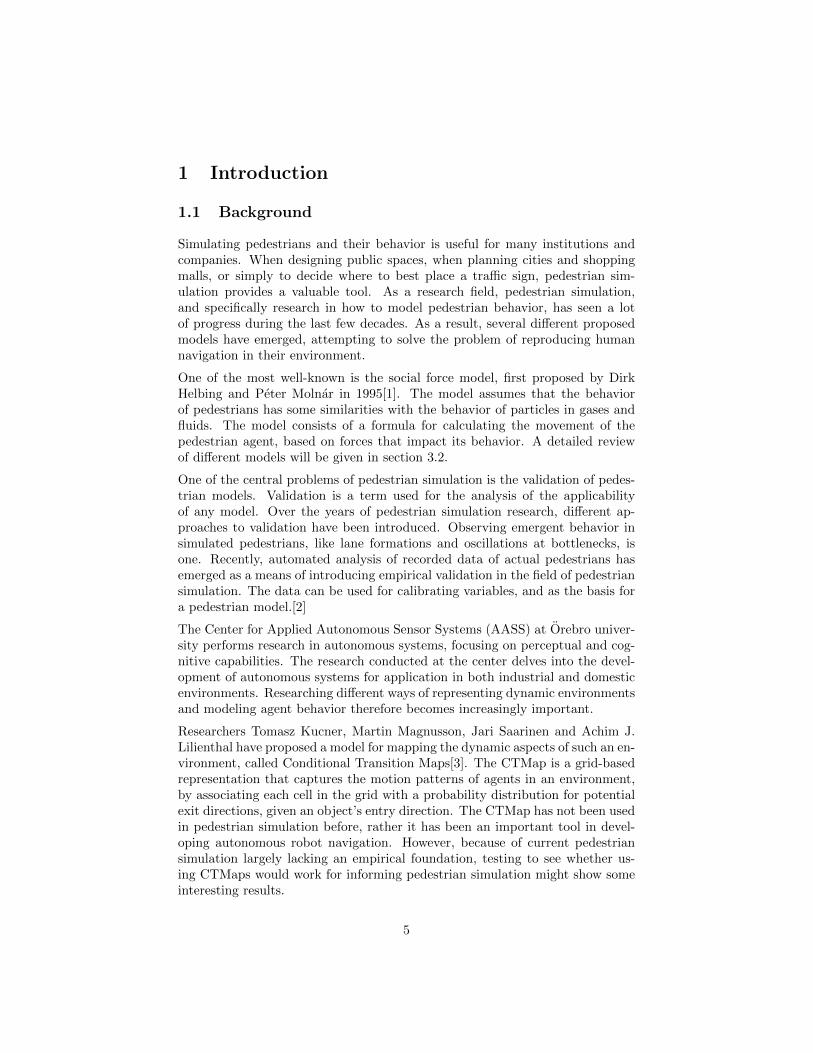
Simulating pedestrians and their behavior is useful for many institutions andcompanies. When designing public spaces, when planning cities and shoppingmalls, or simply to decide where to best place a traffic sign, pedestrian sim-ulation provides a valuable tool. As a research field, pedestrian simulation,and specifically research in how to model pedestrian behavior, has seen a lotof progress during the last few decades. As a result, several different proposedmodels have emerged, attempting to solve the problem of reproducing humannavigation in their environment.
One of the most well-known is the social force model, first proposed by DirkHelbing and Peter Molnar in 1995[1]. The model assumes that the behaviorof pedestrians has some similarities with the behavior of particles in gases andfluids. The model consists of a formula for calculating the movement of thepedestrian agent, based on forces that impact its behavior. A detailed reviewof different models will be given in section 3.2.
One of the central problems of pedestrian simulation is the validation of pedes-trian models. Validation is a term used for the analysis of the applicabilityof any model. Over the years of pedestrian simulation research, different ap-proaches to validation have been introduced. Observing emergent behavior insimulated pedestrians, like lane formations and oscillations at bottlenecks, isone. Recently, automated analysis of recorded data of actual pedestrians hasemerged as a means of introducing empirical validation in the field of pedestriansimulation. The data can be used for calibrating variables, and as the basis fora pedestrian model.[2]
The Center for Applied Autonomous Sensor Systems (AASS) at Orebro univer-sity performs research in autonomous systems, focusing on perceptual and cog-nitive capabilities. The research conducted at the center delves into the devel-opment of autonomous systems for application in both industrial and domesticenvironments. Researching different ways of representing dynamic environmentsand modeling agent behavior therefore becomes increasingly important.
Researchers Tomasz Kucner, Martin Magnusson, Jari Saarinen and Achim J.Lilienthal have proposed a model for mapping the dynamic aspects of such an en-vironment, called Conditional Transition Maps[3]. The CTMap is a grid-basedrepresentation that captures the motion patterns of agents in an environment,by associating each cell in the grid with a probability distribution for potentialexit directions, given an object’s entry direction. The CTMap has not been usedin pedestrian simulation before, rather it has been an important tool in devel-oping autonomous robot navigation. However, because of current pedestriansimulation largely lacking an empirical foundation, testing to see whether us-ing CTMaps would work for informing pedestrian simulation might show someinteresting results.
5
1.2 Project
The thesis constitutes an investigation into the possibilities of a CTMap asthe basis of a model for pedestrian behavior. The comparison with an alreadyestablished model for pedestrian simulation, like the social force model, shallshed light on whether the new model is feasible and can be validated as apedestrian simulation tool. Furthermore, a theoretical background based inexisting research in the field has provided a basis for developing the model andthe different variants of it.
1.3 Objective
The objective of the thesis was to develop a pedestrian simulation model basedon a CTMap and qualitatively assess its validity against a theoretical and prac-tical background.
1.4 Requirements
• Discussing existing pedestrian simulation.
• Implementing the social force model or another prominent pedestrian sim-ulation model for a given scenario.
• Developing a pedestrian simulation where agents utilize a CTMap for mak-ing decisions on their movement direction and step, and qualitatively as-sessing its validity as a model for pedestrian simulation.
• Analyzing and comparing the results from the two models.
6
2 Methods and tools
2.1 Methods
For the project, an adapted form of the SCRUM-method was utilized. Usingthe thesis blog as the main resource for the method, each weekly sprint wasdocumented, dividing tasks into categories, depending if they were future tasks,a work in progress, or finished tasks, respectively. At the beginning of eachweekly sprint, specific tasks were set to be done during that sprint, and thetime consumption for each task was estimated. At the start of the sprint, allof the tasks were categorized as ”to do”. At the start of each day, which taskswere to be undertaken during the day was decided, and moved to the ”doing”-category. Each time a task was finished, it would then finally be documentedas done, by moving it to the corresponding category. In this way the workingprocess was always documented, on a weekly and a daily basis, which enabledfor easy following of the time plan set for the project.
2.2 Tools
For the implementation of the models, SeSAm 2.5.2 (Shell for Simulated AgentSystems, using Java version 7) was used, which is an environment for developingmulti-agent models. The software was provided by the institution. As theformat of the data set which the project is based on was unknown at the startof the project, it was unclear whether SeSAm could be used as it is, needed tobe extended or replaced by some other multiagent platform.
The entire project was completed on computers running Windows 8.1 as theoperative system.
2.3 Resources
The data files used in the project were provided by researchers Tomasz Kucnerand Franziska Klugl of Orebro University. The data consisted of .csv-files, con-taining conditional transition probabilities and pedestrian trajectories, based onanalyzed video data recorded in the Forum at the University of Edinburgh onthe 24th and 25th of August.[4] The data set is described in greater detail insection 4.1.
7
3 Existing research
The following chapter includes a theoretical background for pedestrian simula-tion, and goes into greater detail in specific areas relevant to the project. Thebasics of the Conditional Transition Map are also described.
3.1 Introduction
In the following section, pedestrian simulation, its uses and different forms, willbe discussed. This will form a knowledge base for designing models in laterphases of the project.
Pedestrian simulation has many applications. It provides a useful tool for anyarea where a knowledge of pedestrian and crowd behavior is of use. For example,being able to simulate evacuation situations or testing to see how a plannedchange to infrastructure might affect pedestrian flow, is of interest to both aprivate and a public sector when designing public facilities and spaces.
Depending on the application needs, a pedestrian simulation model needs toreproduce the dynamics of a pedestrian crowd quantitatively, as well as qual-itatively. This means, that the size of a simulation is of importance, as is theamount of pedestrians being simulated. The level of decision making conductedby each pedestrian in the simulation is also central to the requirements set forthe model. For a simulation to be able to provide applicable results, i e resultsthat correspond to the real-world situation being modeled, all of these aspectsneed to be taken into consideration and balanced accordingly - simulating alarge amount of complex pedestrians will require large amounts of computingpower, or will need to accept some simplification.[5, 6]
It has also been discussed whether or not a pedestrian simulation model needsto be able to represent pedestrian behavior in a range of different situations, andnot just modelled to apply in a specific setting, which would make a data-drivenapproach much easier. Depending on the application area, pedestrian modelstend to be either very complex and precise but slow, or fast models where thelevel of behavior displayed by the pedestrians can be put into question.[7]
Different models for pedestrian simulation can be divided into categories, basedon different levels of abstraction, i e granularity. A pedestrian model can beconsidered to be either microscopic, macroscopic or mesoscopic. A microscopicmodel entails that each pedestrian is considered a unique entity, often calledan agent. Each agent has its own properties and decision making abilities, notunlike real-world pedestrians. Macroscopic models, on the other hand, capturepedestrian flow as a whole, without considering each individual pedestrian’s de-cision making and interactions with others, which can simplify the calculationsneeded for the simulation, and lower the computational costs. Lastly, meso-scopic models combine the two previous models, and make use of both models’
8
abilities, describing pedestrian behavior on a microscopic level but not consid-ering them individually. Mesoscopic models are often referred to as gas-kineticmodels.[6, 5]
In addition, pedestrian models can also be categorized based on the detail ofdescription of space. Space can either be discrete or continuous. A discretespace model divides the environment into subspaces, or sets of cells. Each cellhas a cell size which discretizes the environment. In a continuous space modelthe resolution detail of the environment is arbitrary. When the simulation ismade for a specific environment or map, often a discrete space model is used.Time in a model can also be described as either discrete or continuous.[5]
These attributes can be used to characterize existing and future pedestrianmodels. In the following, they will be used to describe several prominent existingmodels.
3.2 Models for pedestrian simulation
3.2.1 Agent-based models
Agent-based models for pedestrian simulation are grounded in the idea of anautonomous, and interacting, agent. It is therefore microscopic in nature. Thiskind of model is useful when a higher level of cognitive behavior and decisionmaking is required or desired. The agents can be designed to possess a capacityfor path-planning, and to adapt to a dynamic environment. In such models itis also possible to integrate interaction between agents, which can enable thesimulation of pedestrian group formation. [6]
Artificial intelligence can be applied to agent-based models, and therefore theycan become quite accurate at reproducing pedestrian behavior. A great ad-vantage of this type of model for pedestrian simulation is that the agent itselfneed not be modified when a change in the environment is made, but rather theagent adapts to the changes autonomously. The agent has the ability to react tochanges to its environment, rather than relying on already known informationabout it. The agent as an abstraction of a pedestrian is also quite intuitive tounderstand and analyze. The disadvantage of an agent-based model lies in thepotential complexity of the model, which can make them difficult to analyze.They also tend to require large amounts of computational power compared tomodels with simpler structures. This becomes increasingly relevant when theobjective is to analyze crowd behavior and large amounts of pedestrians areincluded in the model.[6, 5]
3.2.2 The social force model
The social force model assumes that certain situations, when considering trafficand the movement of pedestrians, becomes routine as a result of them being
9
simple and mainly the result of reacting to the environment. Its basic assump-tion is that the behavior of the pedestrian can be described as a result of forcesinfluencing it to do different things.[1, 8]
The social force model, as an agent-based model, considers each pedestrian anentity with internal motivations that guide its path, and is also microscopicin nature. The difference to other agent-based models is that the social forcemodel describes that motivation as a function of repelling and attracting forces,rather than describing them as a result of cognitive decision making. The socialforce model considers both time and space continuous.[1]
The concept is that a pedestrian is attracted to its desired destination with acertain velocity, and attempts to move towards it. This is the driving force ofthe pedestrian. The motion of the pedestrian is also influenced by a repellingforce, keeping it from moving into other pedestrians or obstacles, like the wallsof buildings. This reflects that pedestrians feel uncomfortable when too close toothers, and also that they prefer not to walk too close to walls. As a third force,a pedestrian has a certain velocity towards additional objects of interest. Thiscorresponds to a person being attracted by interesting events or familiar peoplein its environment. Anything behind the pedestrian is decreasing in interest andrepulsive effect, as it moves further away from it. The model aims at producinga Gaussian distribution of desired walking speeds across all pedestrians. A fluc-tuation term is also introduced, to account for random behavior in ambiguoussituations that might arise - e g when both directions leading around an obsta-cle are equal. Added together these forces describe the movement direction andspeed of each pedestrian in the model.[1]
Simulation using the social force model is able to reproduce pedestrian crowdbehavior like lane formation, herding, and oscillation of walking directions, de-spite the pedestrian behavior being simplified. These kinds of observable crowdformations are used as a means of qualitatively validating the social force model,as it corresponds to how actual pedestrians behave in a real environment.[1]
Due to each entity calculating its forces based on many other pedestrian si-multaneously, and the model often being used for simulating larger crowds ofpedestrians, the model can be quite cumbersome to simulate and requires a lotof computing power. This also makes it difficult to simulate very large crowdsof pedestrians using the model. Balancing the different constants weighting theforces in the equation requires a lot of time and extensive testing, in order toproduce realistic overall behavior. Even small changes to one of the variablesoften requires adjustments in the others. In some cases, the simplification ofpedestrian behavior to social forces produces unrealistic behavior. In sections4.2 and 5.3 the social force model is described in greater detail, as it was se-lected as the established pedestrian model for the comparison to CTM-basedmodel.[5, 6, 8]
10
3.2.3 Cellular automaton models
As opposed to the above described model, the cellular automaton model repre-sents time and space as discrete. Each cell in the model is a representation ofa certain area, which holds information about the environment. The cell canhold information about its neighborhood or in what direction the goal is, forexample. The cell most often contains state information, i e if its occupied ornot. The state is changed using rules based on the current state and the statesof the neighboring cells.[9]
A renown example of a cellular automaton is The Game of Life, created byJohn Conway in 1970. The model showcases emergent patterns that occur witha simple set of rules, and using different starting settings.[10]
In CA-based pedestrian simulation models the cell state represents informationabout only one pedestrian. For example, the destination goal of the pedestrianscan be added to the cell state information. This way, the pedestrian will beguided, cell by cell, towards its goal; and the path of the pedestrian can beobserved by analyzing the changes in cell state. The size of the neighborhood,whether a Moore or a Von Neumann-neighborhood, determines the outcome ofthe simulation to great extent. Each pedestrian agent is updated in parallel toeach other, and moves to a neighboring cell.[8]
A model that is especially applicable to pedestrian and traffic simulation isthe Blue and Adler model.[11] It applies a multi-lane variant of agent move-ment, where each pedestrian is updated in four synchronous steps. A pedestrianchooses a lane, and performs possible change of lane. After this, each pedestrianagent determines its velocity based on the space and possible congestion in thelane it is in. In the fourth step, each pedestrian moves accordingly based onits set velocity. In this variant of the cellular automaton each pedestrian can,depending on its set velocity, move different numbers of cells for each time step,not just one a time. Pedestrians approaching each other and going in oppositedirections can also exchange positions, to avoid collisions.[11]
Another variant of the cellular automaton model is the floor-field model.[12]One of the determining factors of pedestrian movement in the floor-field modelis a virtual trace, based on chemotaxis. Chemotaxis is used by insects like antsfor communication, where they leave a chemical trace guiding other ants to foodand other points of interest outside the colony. Drawing inspiration from thisnatural phenomenon the floor-field model provides a more dynamic version ofthe cellular automaton model for pedestrian simulation. In it each pedestrianagent leaves a virtual trace in the environment, influencing the transition prob-abilities of the cell. In practice this means that transitions used by pedestriansmore often grow stronger with time, influencing the motion of other pedestriansin turn. Each agent will at random choose its next cell based on the transitionprobabilities. The model also includes a formula for diffusing and decaying thetrace over a period of time, so that transition probabilities become weaker if notused for a certain period of time.[12]
11
3.3 Data-Driven pedestrian simulation
What has been largely lacking and very limiting in the field of pedestrian sim-ulation is empirical data. This is due to the fact that pedestrian simulationhas a long history in evacuation dynamics, and trying out viable scenarios withlarge amounts of people in a stressful situation is both costly and potentiallydangerous.
Over the past decade, the collection and usage of empirical data on pedestrianbehavior has grown along with the technical advancements made in automatedvideo processing and computational power. The availability of data provides abase to build better validated models for pedestrian simulation. Empirical datacan also be used for calibrating pedestrian models for particular scenarios andapplication areas. With the help of motion tracking, trajectories of individualpedestrians can be determined, and used as a basis for simulation, and also asa means of validation through comparison.[2, 8]
3.4 Conditional Transition Maps
3.4.1 Background
The Conditional Transition Map[3] is a grid-based representation of the dynam-ics of an environment. The model originates in the field of robotics as a means ofnavigation for mobile robots in human environments. Traditionally, occupancygrid maps have been utilized for probabilistic environment representation, ag-gregating how probable it is to encounter a human at a particular location.however, these do not account for dynamic elements in an environment. By as-suming that the motion of dynamic objects is continuous, local neighborhoodsof cells in the grid map become central for the analysis of the changes in theenvironment. Furthermore, it can be observed that when an object enters apreviously empty cell, it must have come from a neighboring cell, and will alsoexit into one of the neighboring cells.[3]
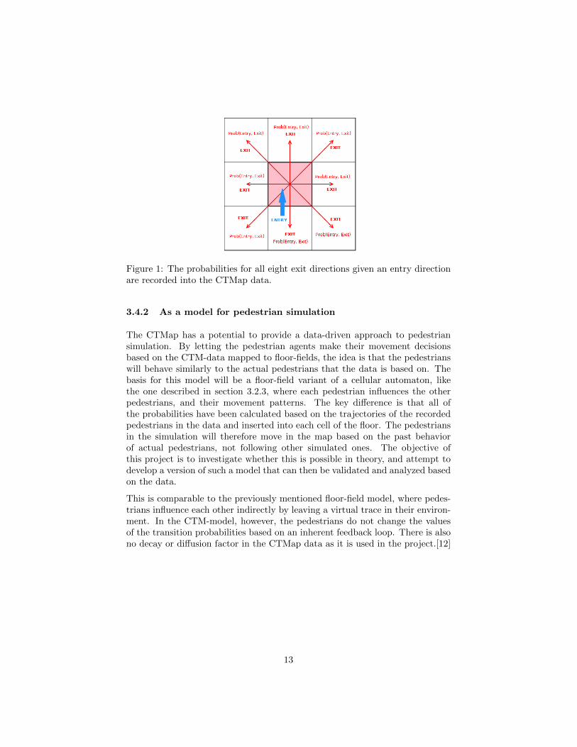
Each cell in the map has an occupancy state, which holds a 1 if it is occupiedby an object or a 0 if it is empty. A cell will store probabilities for all possibletransitions, based on recorded trajectories of dynamic objects. This resultsin each cell having 8 sets of 8 variables, one for each pair of entry and exitdirections. Each variable holds the probability of that particular transitionoccurring, as shown in figure 1 below. The probability is the result of dividingthe number of exits in a certain direction by the total amount of entries to acell from a certain direction. [3]
12
Figure 1: The probabilities for all eight exit directions given an entry directionare recorded into the CTMap data.
3.4.2 As a model for pedestrian simulation
The CTMap has a potential to provide a data-driven approach to pedestriansimulation. By letting the pedestrian agents make their movement decisionsbased on the CTM-data mapped to floor-fields, the idea is that the pedestrianswill behave similarly to the actual pedestrians that the data is based on. Thebasis for this model will be a floor-field variant of a cellular automaton, likethe one described in section 3.2.3, where each pedestrian influences the otherpedestrians, and their movement patterns. The key difference is that all ofthe probabilities have been calculated based on the trajectories of the recordedpedestrians in the data and inserted into each cell of the floor. The pedestriansin the simulation will therefore move in the map based on the past behaviorof actual pedestrians, not following other simulated ones. The objective ofthis project is to investigate whether this is possible in theory, and attempt todevelop a version of such a model that can then be validated and analyzed basedon the data.
This is comparable to the previously mentioned floor-field model, where pedes-trians influence each other indirectly by leaving a virtual trace in their environ-ment. In the CTM-model, however, the pedestrians do not change the valuesof the transition probabilities based on an inherent feedback loop. There is alsono decay or diffusion factor in the CTMap data as it is used in the project.[12]
13
4 Design
This chapter describes the underlying design of both models, as well as theintentions for potential future additions and changes to them. Chapter 5 goesinto more detail regarding the implementation process itself, and which practicalsteps were taken in building them.
4.1 The data
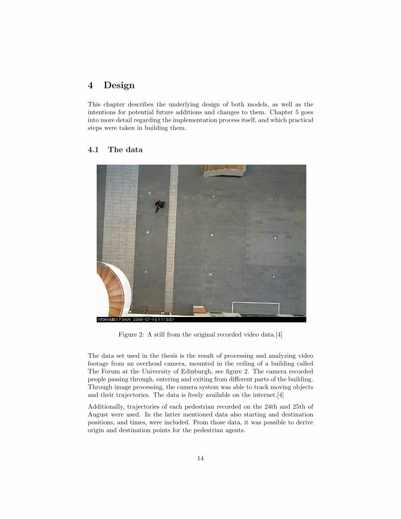
Figure 2: A still from the original recorded video data.[4]
The data set used in the thesis is the result of processing and analyzing videofootage from an overhead camera, mounted in the ceiling of a building calledThe Forum at the University of Edinburgh, see figure 2. The camera recordedpeople passing through, entering and exiting from different parts of the building.Through image processing, the camera system was able to track moving objectsand their trajectories. The data is freely available on the internet.[4]
Additionally, trajectories of each pedestrian recorded on the 24th and 25th ofAugust were used. In the latter mentioned data also starting and destinationpositions, and times, were included. From those data, it was possible to deriveorigin and destination points for the pedestrian agents.
14
Out of the information provided by the data set the resolution and cell size wereset for both models, and the map was generated to resemble the actual layoutof the Forum. Tomasz Kucner created a CTMap from the data on the 24 ofAugust and provided me with it.
Below, in figures 3 and 4, the two data sets, containing the CTMap transitionprobabilities, the pedestrian trajectories and the origin and destination pointshave been visualized into a map.
The pink cells represent cells that have transition probabilities stored into them.The blue ones are cells completely without CTMap data or transition proba-bilities, which in most cases correspond to where obstacles are situated in theForum. This means that no objects or persons moved through those areas onthe 24th of August.
The different colored dots correspond to the trajectories of each pedestrian, fromorigin to destination point.
In figure 3 below, the trajectories recorded on the 24th have been drawn ontothe CTMap from that same date. This can be seen from that the trajectoriescorrespond to the pink cells in the map.
Figure 3: Trajectories recorded on the 24th of August.
It is notable that the trajectories for the 24th of August are quite erratic. Theclusters of dots correspond to pedestrians stopping for a long period of time.There is one pedestrian who moved towards the center of the map and thendecided to go back to its origin. Also, when comparing to the trajectories of the25th the trajectories seem very widely dispersed across the area of the map. Howthese kinds of aspects of the trajectories, and also the transition probabilitiesthemselves, will affect the result of the model development remains to be seen.
15
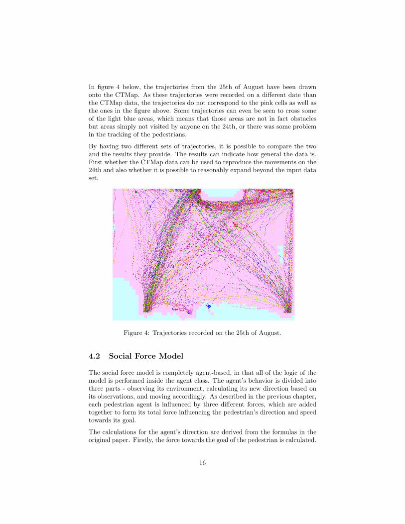
In figure 4 below, the trajectories from the 25th of August have been drawnonto the CTMap. As these trajectories were recorded on a different date thanthe CTMap data, the trajectories do not correspond to the pink cells as well asthe ones in the figure above. Some trajectories can even be seen to cross someof the light blue areas, which means that those areas are not in fact obstaclesbut areas simply not visited by anyone on the 24th, or there was some problemin the tracking of the pedestrians.
By having two different sets of trajectories, it is possible to compare the twoand the results they provide. The results can indicate how general the data is.First whether the CTMap data can be used to reproduce the movements on the24th and also whether it is possible to reasonably expand beyond the input dataset.
Figure 4: Trajectories recorded on the 25th of August.
4.2 Social Force Model
The social force model is completely agent-based, in that all of the logic of themodel is performed inside the agent class. The agent’s behavior is divided intothree parts - observing its environment, calculating its new direction based onits observations, and moving accordingly. As described in the previous chapter,each pedestrian agent is influenced by three different forces, which are addedtogether to form its total force influencing the pedestrian’s direction and speedtowards its goal.
The calculations for the agent’s direction are derived from the formulas in theoriginal paper. Firstly, the force towards the goal of the pedestrian is calculated.
16
Each agent strives to move towards its destination point in a straight line fromits origin, moving with a preferred speed υ0
α, defined by the equation below(1).The desired velocity is defined by υ0
αeα, υα defines the deviation from thatvelocity due to any avoidance behavior and τα corresponds to the relaxationtime within which the agent approaches its destination.
(1) F 0α = τα(υ
0αeα − υα)
When adding the objective force to the total force, the result from this formulais weighted using a constant parameter.
The agent will keep a certain distance to other pedestrians and any observedobstacles. It is influenced by a repulsive force for avoiding other pedestriansin its surroundings and avoiding collisions, seen in the equation below(2). rαβis the distance between the agent and the other pedestrian, and Vαβ is therepulsive potential of that pedestrian.
(2) fαβ(rαβ) = −∇rαβVαβ [b(rαβ)]
This is calculated by assuming that each pedestrian has a personal space aroundit, shaped like an ellipse and denoted by the semiminor axis of the ellipse b(rαβ).The ellipse is elongated in front of the agent, to allow for movement. b(rαβ) iscalculated as seen in the equation below(3). υβ∆t denotes the order of the stepwidth of the other pedestrian.
(3) b(rαβ) =
√(‖rαβ‖+‖rαβ−υβ∆teβ‖)2−(υβ∆t)2
2
Pedestrians will also avoid walls and other obstacles, and here the formula dif-fers from the repulsive force of other pedestrians, because it is assumed thatthese obstacles do not move. Therefore, the ellipse is not calculated for thisforce. Instead, the closest point of the wall to the agent is used to calculate therepulsive force to that obstacle, see the equation below(4). Here rαB denotesthe distance from the agent to the closest point on the obstacle.[1]
(4) FαB(rαB) = −∇rαBUαB(‖rαB‖)
4.3 CTM-Based Model
In contrast to the social force model, the CTM-based agent draws its logic fromthe data set. This results in an agent structure that is a lot simpler in its mostbasic form than the social force pedestrian. In the first variant of the CTM-model the pedestrians simply follow the highest transition probability giventheir entry direction. They do not attempt to head towards their respectivedestinations. This is mainly to see whether they would actually find their wayat all simply by using the data. It was expected that this would not be enoughfor the pedestrians to reach their goal points, and especially not in the traveltime based on the starting and destination times from the data set. This agentlogic results in most of the data remaining unused.
17
4.3.1 Variants of the model
As described in previous chapters, the objective of the project was to developa CTM-based, data-driven model for pedestrian simulation. This includes aninvestigation into what kind of behavior the data itself can produce, and whatkind of logic the agent itself needs to have to produce good pedestrian behav-ior. A desired result of the model development is that the trajectories of thepedestrian agents are as similar as possible to those of the pedestrians’ recordedin the data. Another aspect to consider is to develop a model based on thedata that is general enough to produce valid results even when the input datais changed. Therefore an investigation into the possibilities of further developedversions of the pedestrian agent is important for the project.
4.3.2 Roulette wheel
The first step in further developing the model is trying to incorporate all ofthe data into the decision-making of the pedestrian agent. This was done bychoosing an exit direction randomly, based on the probabilities for its specificentry direction. This way all of the directions are a possible result, but thedirection probabilities are proportionally weighted. In this variant the behaviorof the pedestrians is also completely based on the data itself.
4.3.3 Heading towards the destination
The conditional transition probabilities themselves do not take into considera-tion where each pedestrian is heading, and can therefore not produce a resultwhere all the pedestrians end up at their preferred goal points. As an actualpedestrian will always keep its destination in mind, so must the simulated agent.As seen in the social force model, the desire to head in the direction of the desti-nation should be the most driving force. Because the pedestrians recorded intothe data have different destinations, a general floor-field map by itself might notbe a sufficient solution.
By implementing a variant of the pedestrian agent that uses a calculation of apreferred direction based on its ultimate destination, similar to that of the socialforce agent, it is possible to achieve a result that resembles the pedestrians inthe data set. Similar to that of the previous version, this one can, for example,use the destination as a weight for the exit directions that point in the preferreddirection. Below (5) is the equation used to calculate the total probability forthe exit in the direction of the agent’s destination, where α denotes the weightconstant and d is the transition probability.
(5) dfinal = α ∗ dctm + (1− α) ∗ ddest
18
4.3.4 Considering past movement
While randomly choosing an exit direction works in favor of those with highertransition probabilities, it is still possible that a pedestrian will walk back andforth between two cells. This is hardly a behavior seen in actual pedestrians.To lower the likelihood of this occurring, the pedestrian can store all of its pastpositions in a movement history. Similarly to that of the destination weight,the pedestrian can then lower the probability of the exit direction pointing toan already visited cell, especially the one it just came from. A problem thatmight arise from this is that a pedestrian can get stuck in a narrow hallway ora dead end that it was lead to by the probabilities.
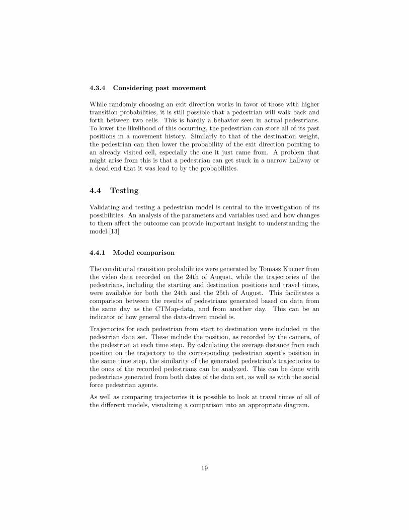
4.4 Testing
Validating and testing a pedestrian model is central to the investigation of itspossibilities. An analysis of the parameters and variables used and how changesto them affect the outcome can provide important insight to understanding themodel.[13]
4.4.1 Model comparison
The conditional transition probabilities were generated by Tomasz Kucner fromthe video data recorded on the 24th of August, while the trajectories of thepedestrians, including the starting and destination positions and travel times,were available for both the 24th and the 25th of August. This facilitates acomparison between the results of pedestrians generated based on data fromthe same day as the CTMap-data, and from another day. This can be anindicator of how general the data-driven model is.
Trajectories for each pedestrian from start to destination were included in thepedestrian data set. These include the position, as recorded by the camera, ofthe pedestrian at each time step. By calculating the average distance from eachposition on the trajectory to the corresponding pedestrian agent’s position inthe same time step, the similarity of the generated pedestrian’s trajectories tothe ones of the recorded pedestrians can be analyzed. This can be done withpedestrians generated from both dates of the data set, as well as with the socialforce pedestrian agents.
As well as comparing trajectories it is possible to look at travel times of all ofthe different models, visualizing a comparison into an appropriate diagram.
19
5 Implementation
The following chapter describes how the development concepts from the previouschapter were put into practice, and what functionalities within the developmentenvironment were used to implement the pedestrian models. Some visualizationof the agent structures is included to further describe what was done.
5.1 SeSAm
For the implementation and development of the pedestrian models the devel-opment environment SeSAm (Shell for Simulated Agent Systems) was used.SeSAm provides a visual approach to programming agent-based simulations.Several models of different biological and other systems are included as modellibraries.[14]
For visualizing two-dimensional simulations, SeSAm is very intuitive to use.This was the primary reason for choosing the platform for the project. Whilevisual validation is not in itself central to pedestrian simulation, it greatly facil-itates the development. It is intuitive to understand that a pedestrian is a circlemoving in a rectangular map, and this makes it easy to see, where changes needto be made.
5.1.1 Plugins
For implementing the CTM-based models, the data was the most central part.While the default version of SeSAm does not support importing and parsingcomma-separated value-files, there are plugins available that do. The ones usedin the project were FileOperations and 2DSpatial.
FileOperations adds the functionality of handling files to SeSAm. It was usedfor importing the relevant data files into the project model.
The high level 2DSpatial-plugin provides functions for tokenizing strings, whichwas needed in the project for extracting the data from the data files.
5.2 Data Import and Map Generation
All of the data handling occurs in the world-class, i e the map of the environment.Utilizing the SeSAm-plugins mentioned previously, the data files are imported,parsed and stored in global variables.
The map is then generated based on the resolution of the map in the data set,and filled with cells. By matching cells in the data with the ones in the generatedmap, the transition probabilities are stored in their corresponding locations.
20
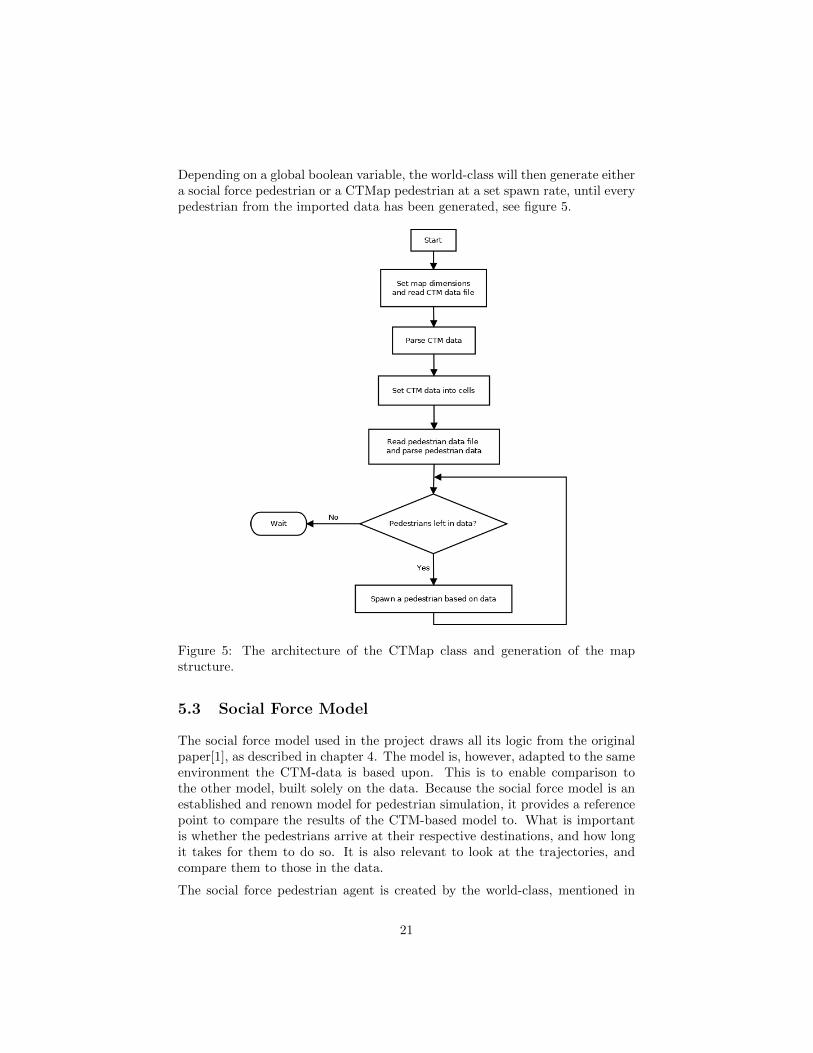
Depending on a global boolean variable, the world-class will then generate eithera social force pedestrian or a CTMap pedestrian at a set spawn rate, until everypedestrian from the imported data has been generated, see figure 5.
Figure 5: The architecture of the CTMap class and generation of the mapstructure.
5.3 Social Force Model
The social force model used in the project draws all its logic from the originalpaper[1], as described in chapter 4. The model is, however, adapted to the sameenvironment the CTM-data is based upon. This is to enable comparison tothe other model, built solely on the data. Because the social force model is anestablished and renown model for pedestrian simulation, it provides a referencepoint to compare the results of the CTM-based model to. What is importantis whether the pedestrians arrive at their respective destinations, and how longit takes for them to do so. It is also relevant to look at the trajectories, andcompare them to those in the data.
The social force pedestrian agent is created by the world-class, mentioned in
21
section 5.2 and placed in the same map as the CTM-pedestrians, describedbelow. It receives a starting point and sets its goal point based on the parsedfile of pedestrian data. The travel time for the recorded pedestrians in the datais also calculated and stored in the agent, to provide a point of reference for thetime step the pedestrian arrives at its destination, and a base for data analysislater on in the project.
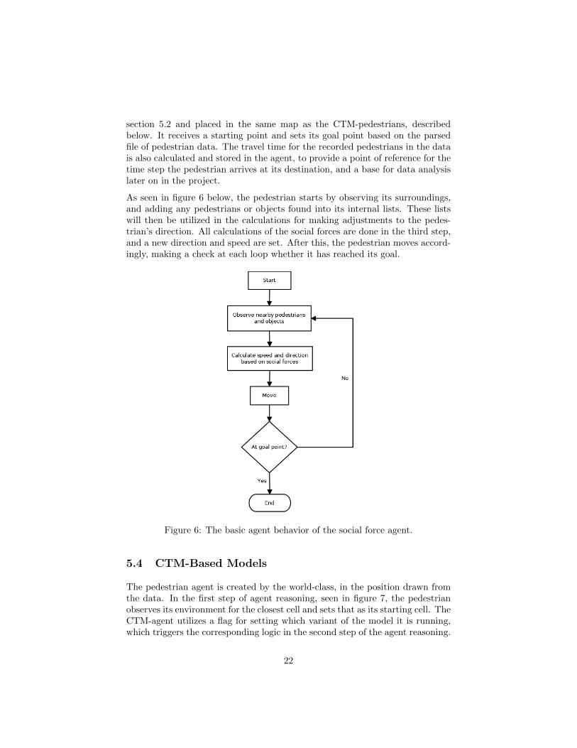
As seen in figure 6 below, the pedestrian starts by observing its surroundings,and adding any pedestrians or objects found into its internal lists. These listswill then be utilized in the calculations for making adjustments to the pedes-trian’s direction. All calculations of the social forces are done in the third step,and a new direction and speed are set. After this, the pedestrian moves accord-ingly, making a check at each loop whether it has reached its goal.
Figure 6: The basic agent behavior of the social force agent.
5.4 CTM-Based Models
The pedestrian agent is created by the world-class, in the position drawn fromthe data. In the first step of agent reasoning, seen in figure 7, the pedestrianobserves its environment for the closest cell and sets that as its starting cell. TheCTM-agent utilizes a flag for setting which variant of the model it is running,which triggers the corresponding logic in the second step of the agent reasoning.
22
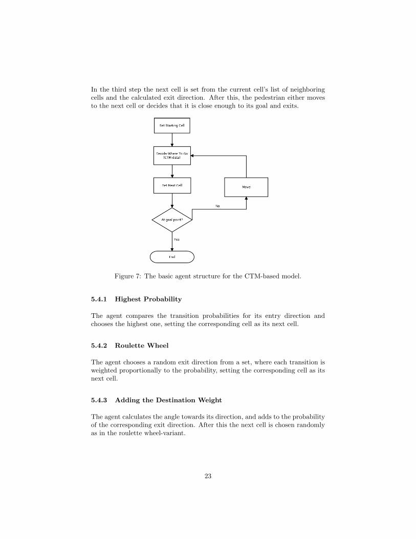
In the third step the next cell is set from the current cell’s list of neighboringcells and the calculated exit direction. After this, the pedestrian either movesto the next cell or decides that it is close enough to its goal and exits.
Figure 7: The basic agent structure for the CTM-based model.
5.4.1 Highest Probability
The agent compares the transition probabilities for its entry direction andchooses the highest one, setting the corresponding cell as its next cell.
5.4.2 Roulette Wheel
The agent chooses a random exit direction from a set, where each transition isweighted proportionally to the probability, setting the corresponding cell as itsnext cell.
5.4.3 Adding the Destination Weight
The agent calculates the angle towards its direction, and adds to the probabilityof the corresponding exit direction. After this the next cell is chosen randomlyas in the roulette wheel-variant.
23
5.4.4 Considering past movement
Due to time constraints for the project the history weight was not implemented.
24
6 Results
In the following chapter the results of the model implementations are describedand discussed. Simulations were conducted using pedestrian data from both the24th and the 25th of August in all cases, for all the different models. By usingscreenshots of the pedestrian trajectories and diagrams displaying the results ofthe simulations numerically, the different models are compared to each other.These kinds of visualizations of the results facilitate analysis of the differentvariants of CTM-based models, as was evident during project development.
Screenshots of the simulations provide insight into how the models work and dif-fer from each other, especially when considering the CTM-based models, wherethe behavior is largely unknown until the simulation is run and displayed in thismanner.
6.1 Social Force Model
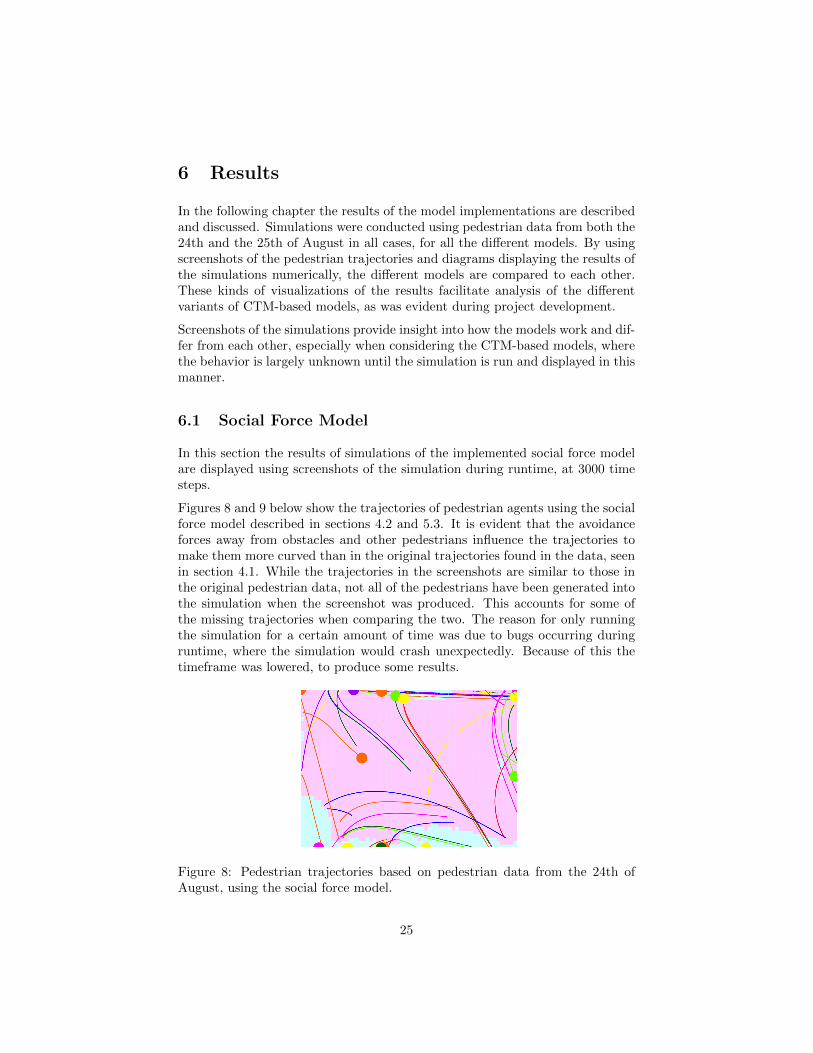
In this section the results of simulations of the implemented social force modelare displayed using screenshots of the simulation during runtime, at 3000 timesteps.
Figures 8 and 9 below show the trajectories of pedestrian agents using the socialforce model described in sections 4.2 and 5.3. It is evident that the avoidanceforces away from obstacles and other pedestrians influence the trajectories tomake them more curved than in the original trajectories found in the data, seenin section 4.1. While the trajectories in the screenshots are similar to those inthe original pedestrian data, not all of the pedestrians have been generated intothe simulation when the screenshot was produced. This accounts for some ofthe missing trajectories when comparing the two. The reason for only runningthe simulation for a certain amount of time was due to bugs occurring duringruntime, where the simulation would crash unexpectedly. Because of this thetimeframe was lowered, to produce some results.
Figure 8: Pedestrian trajectories based on pedestrian data from the 24th ofAugust, using the social force model.
25
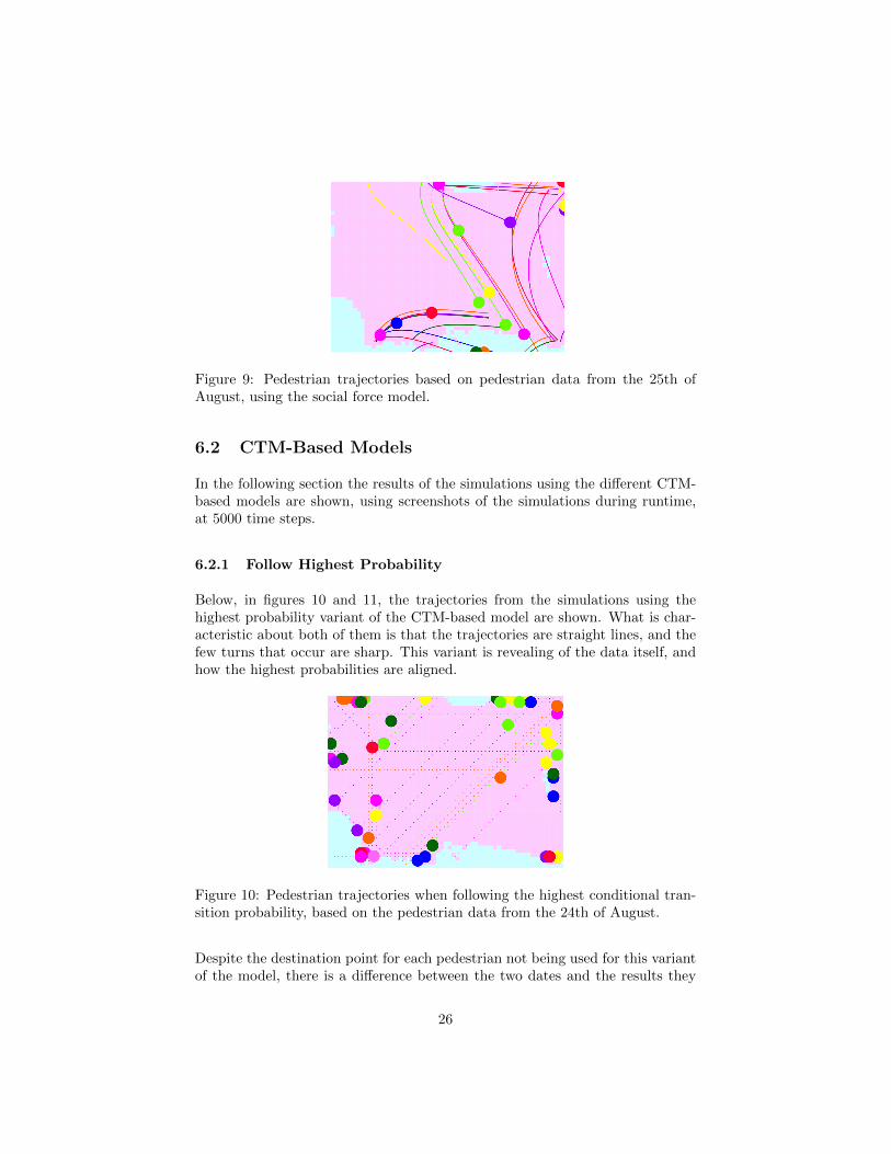
Figure 9: Pedestrian trajectories based on pedestrian data from the 25th ofAugust, using the social force model.
6.2 CTM-Based Models
In the following section the results of the simulations using the different CTM-based models are shown, using screenshots of the simulations during runtime,at 5000 time steps.
6.2.1 Follow Highest Probability
Below, in figures 10 and 11, the trajectories from the simulations using thehighest probability variant of the CTM-based model are shown. What is char-acteristic about both of them is that the trajectories are straight lines, and thefew turns that occur are sharp. This variant is revealing of the data itself, andhow the highest probabilities are aligned.
Figure 10: Pedestrian trajectories when following the highest conditional tran-sition probability, based on the pedestrian data from the 24th of August.
Despite the destination point for each pedestrian not being used for this variantof the model, there is a difference between the two dates and the results they
26
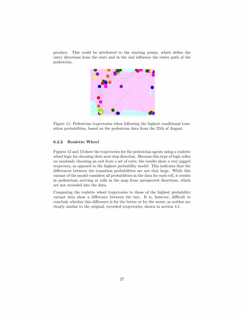
produce. This could be attributed to the starting points, which define theentry directions from the start and in the end influence the entire path of thepedestrian.
Figure 11: Pedestrian trajectories when following the highest conditional tran-sition probabilities, based on the pedestrian data from the 25th of August.
6.2.2 Roulette Wheel
Figures 12 and 13 show the trajectories for the pedestrian agents using a roulettewheel logic for choosing their next step direction. Because this type of logic relieson randomly choosing an exit from a set of exits, the results show a very jaggedtrajectory, as opposed to the highest probability model. This indicates that thedifferences between the transition probabilities are not that large. While thisvariant of the model considers all probabilities in the data for each cell, it resultsin pedestrians arriving at cells in the map from unexpected directions, whichare not recorded into the data.
Comparing the roulette wheel trajectories to those of the highest probabilityvariant does show a difference between the two. It is, however, difficult toconclude whether this difference is for the better or for the worse, as neither areclearly similar to the original, recorded trajectories, shown in section 4.1.
27
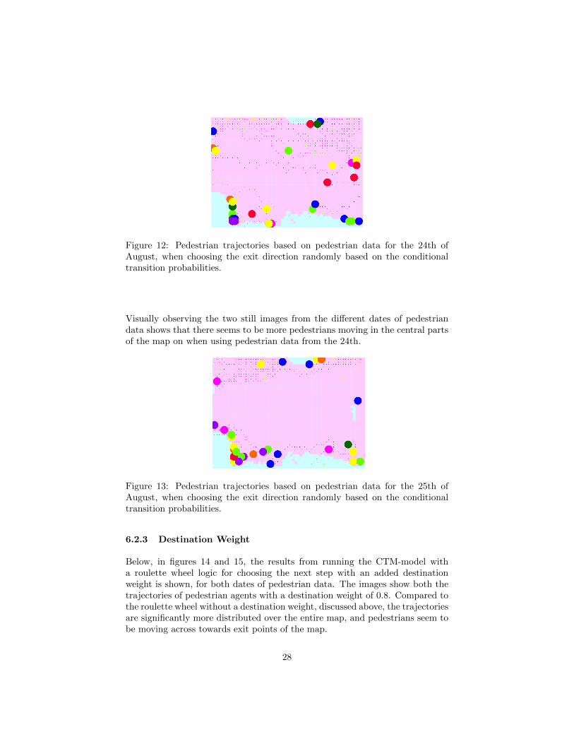
Figure 12: Pedestrian trajectories based on pedestrian data for the 24th ofAugust, when choosing the exit direction randomly based on the conditionaltransition probabilities.
Visually observing the two still images from the different dates of pedestriandata shows that there seems to be more pedestrians moving in the central partsof the map on when using pedestrian data from the 24th.
Figure 13: Pedestrian trajectories based on pedestrian data for the 25th ofAugust, when choosing the exit direction randomly based on the conditionaltransition probabilities.
6.2.3 Destination Weight
Below, in figures 14 and 15, the results from running the CTM-model witha roulette wheel logic for choosing the next step with an added destinationweight is shown, for both dates of pedestrian data. The images show both thetrajectories of pedestrian agents with a destination weight of 0.8. Compared tothe roulette wheel without a destination weight, discussed above, the trajectoriesare significantly more distributed over the entire map, and pedestrians seem tobe moving across towards exit points of the map.
28
Figure 14: Pedestrian trajectories based on pedestrian data from the 24th ofAugust, using a destination weight.
Visually there is quite a big difference between the two dates of pedestrian data.The trajectories seem to be focused around the exits in both cases, however.
Figure 15: Pedestrian trajectories based on pedestrian data from the 25th ofAugust, using a destination weight.
6.3 Model Comparison
The trajectories shown above, in sections 6.1 and 6.2, display the behavior ofthe pedestrian agents in the different models. All of them differ from each other,and none of them look clearly similar to original trajectories, shown in section4.1. While comparing trajectories can provide a valuable tool for validation,comparing the models numerically provides another kind of perspective into theresults of the simulations, more precisely analyzable.
Below follows a summary of data analysis and comparison that was conducted,using the original data set and comparing the numbers to the results of allthe models. The social force model and its results have also been included, toprovide a frame of reference for the CTM-based models.
29
The first aspect that was compared was the percentage of pedestrians reachingtheir destinations. The destinations were all, as described in section 4.1, basedon the original data set, including both the 24th and the 25th of August. Usingthe logic of the different variants of models each pedestrian agent attempted toreach its set destination point that was based on an actual recorded pedestrian.The error margin for the agents reaching their destination is quite small, theyhave to be less than two cells away from their goal position to be consideredhaving arrived at their destination. This applies to all models.
Each simulation for each variant of model was run ten times to produce thedata shown in the diagrams below. In figures 16 and 17 below, the results aredisplayed.
Figure 16: Mean percentage and standard deviation of pedestrians reachingtheir respective destinations for the different models.
From the above figure, it is clear that the agents using the social force modeland not the CTMap were more successful at reaching their destinations - forboth the dates, the result was higher than 25%. There is a small differencebetween the two dates, which can be attributed to the fact that the obstacles inthe map correspond to the gaps in the data in the CTMap, not the pedestriandata.
The second best variant was the destination weight of 0.8 based on data fromthe 24th at just below 5% reaching their destinations. This shows that a largeportion of the pedestrians never reached their destinations.
30
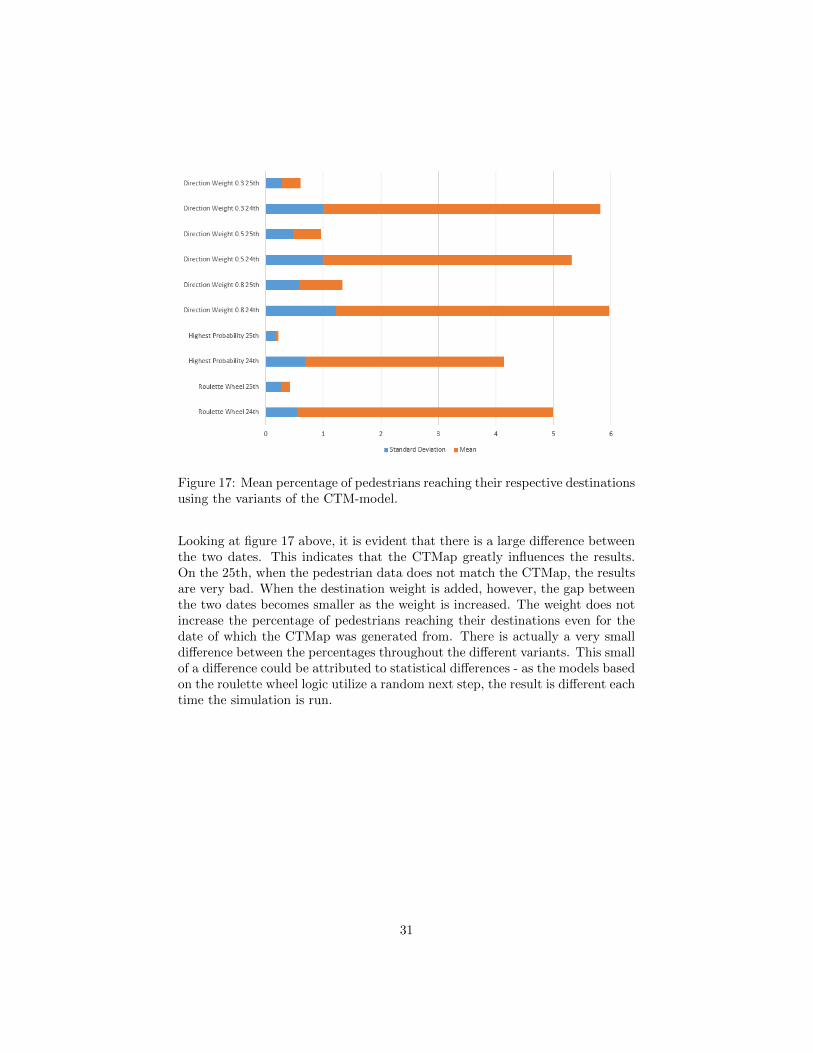
Figure 17: Mean percentage of pedestrians reaching their respective destinationsusing the variants of the CTM-model.
Looking at figure 17 above, it is evident that there is a large difference betweenthe two dates. This indicates that the CTMap greatly influences the results.On the 25th, when the pedestrian data does not match the CTMap, the resultsare very bad. When the destination weight is added, however, the gap betweenthe two dates becomes smaller as the weight is increased. The weight does notincrease the percentage of pedestrians reaching their destinations even for thedate of which the CTMap was generated from. There is actually a very smalldifference between the percentages throughout the different variants. This smallof a difference could be attributed to statistical differences - as the models basedon the roulette wheel logic utilize a random next step, the result is different eachtime the simulation is run.
31
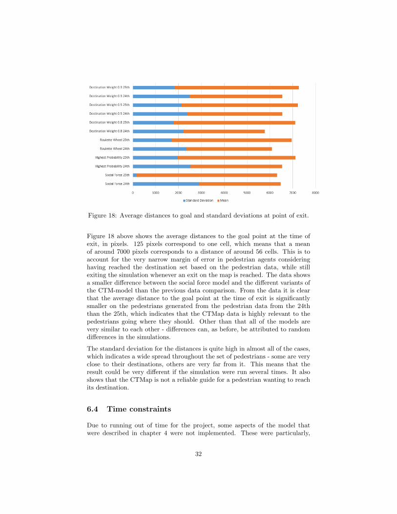
Figure 18: Average distances to goal and standard deviations at point of exit.
Figure 18 above shows the average distances to the goal point at the time ofexit, in pixels. 125 pixels correspond to one cell, which means that a meanof around 7000 pixels corresponds to a distance of around 56 cells. This is toaccount for the very narrow margin of error in pedestrian agents consideringhaving reached the destination set based on the pedestrian data, while stillexiting the simulation whenever an exit on the map is reached. The data showsa smaller difference between the social force model and the different variants ofthe CTM-model than the previous data comparison. From the data it is clearthat the average distance to the goal point at the time of exit is significantlysmaller on the pedestrians generated from the pedestrian data from the 24ththan the 25th, which indicates that the CTMap data is highly relevant to thepedestrians going where they should. Other than that all of the models arevery similar to each other - differences can, as before, be attributed to randomdifferences in the simulations.
The standard deviation for the distances is quite high in almost all of the cases,which indicates a wide spread throughout the set of pedestrians - some are veryclose to their destinations, others are very far from it. This means that theresult could be very different if the simulation were run several times. It alsoshows that the CTMap is not a reliable guide for a pedestrian wanting to reachits destination.
6.4 Time constraints
Due to running out of time for the project, some aspects of the model thatwere described in chapter 4 were not implemented. These were particularly,
32
the CTM-variant utilizing a movement history and the comparison betweenmean travel times for the different models. As described above in sections 6.1and 6.2, the time steps used for the social force model and the variants forthe CTM-models are different. This was due to problems of the social forcesimulation often crashing before reaching 5000 steps, and despite attempting tosolve the problem by debugging the problem persists. It was important that allten runs of the model simulation for producing the data were run for the sameamount of time.
33
7 Discussion
7.1 Compliance with project requirements
All of the requirements for the project, specified in section 1.4, were met. Aninvestigation into the possibilities of using a CTMap as a base for a pedes-trian simulation model was conducted, and compared against a theoretical back-ground of pedestrian simulation. Relevant pedestrian simulation models wereimplemented, using SeSAm, and the results of the simulations were analyzed,compared, and discussed.
Given a longer time frame, other variants of the model could have been imple-mented. Further analysis of the data and why the results are what they arewould also had been the next step in the project.
7.2 Special results and conclusions
The results described in chapter 6 discussing whether or not basing a pedestrianmodel on a CTMap can be validated as a pedestrian simulation tool are incon-clusive. It is evident, based on those results, that for the behavior to be similarto actual pedestrians or even to those of another, established pedestrian simu-lation model, some aspects of the whole, i e the data and the model together,need to be adjusted and worked on.
While some of the pedestrians do reach their destinations using the CTMap,others clearly do not end up close to their goals. Considering the appearance ofthe trajectories of the CTM-agents based on the roulette wheel logic, describedin section 6.2.2, there are large gaps in the data as pedestrians approach fromunexpected directions. This will inevitably lead to them getting lost and notreaching their destinations, which the results indicate.
While taking all transition probabilities into account and randomly choosing anexit direction, as in the roulette wheel approach, does utilize all of the existingdata, it leads to some of the pedestrians going in directions they do not intendto. Adding a destination weight changes the result only marginally.
What is also surprising about the results is that when looking at the distancesto goal, the differences between the different variants of the CTM-based modelsis smaller than the standard deviations. Any differences can therefore be at-tributed to statistical errors. This indicates that the variants of the model donot necessarily produce better results at all.
Based on the result of the project, the CTMap used in the project does notprovide a reliable base on which to build a pedestrian simulation model. Inves-tigating why is the natural next step in development. While the results indicatethat there is still a lot left to work on for the model to produce good behavior,the potential of developing a data-driven pedestrian model is worth exploringfurther.
34
7.3 Further development of the project
The project could be further developed by exploring what results differentchanges to the data set can produce. The first step would be to try a dif-ferent date for the CTMap itself, and comparing the results it produces to theones shown in the project. Additionally, it might be interesting to see if havingdata for all entry directions to each cell would produce different results. Thiscould be achieved by combining data from several dates of recorded video data,for example.
Other variants to the CTM-model could also be developed, starting with thehistory weight for past movement. Finding a way of reducing the stochasticityof the model is central. Using the project’s results as a frame of reference forfuture developments can prove very useful.
7.4 Reflections on own learning
7.4.1 Knowledge and comprehension
At the start of the project I had very little insight into the field of pedestriansimulation. A large part of the project consisted of acquiring an understandingof pedestrian simulation as a research field and the theoretical background es-sential to the project. After working on the project, I have a deeper knowledgeof the history of the field, and also a comprehension of what challenges the fieldis facing at the moment. By then applying what I had learned and implementinga model based on it, the limitations and difficulties that the field faces becamevery real to me.
7.4.2 Proficiency and ability
Indisputably, the biggest learning experience of the project has been working onthe project independently for such a long time. Managing my time and planningtasks for each week was a challenge, but by the end of the project I had learnedhow long each task would take and how to allocate my resources. Being able toundertake similar projects in the future and working independently is a valuableability.
7.4.3 Values and attitude
Another very enlightening aspect of the project is the insight gained into thework process of the faculty and researchers of the institution. Having weeklymeetings and contact with my supervisor, who, at the same time, was my em-ployer for the project, was vital to the process. I also had the opportunityto meet and discuss the project and the data with the original author of the
35
CTMap paper[3], Tomasz Kucner, which gave another perspective of the pro-fessional environment at the institution.
36
References
[1] Helbing D, Molnar P. Social force model for pedestrian dynamics. PhysicalReview E. 1995;51(5):4282–4286.
[2] Teknomo K. Microscopic pedestrian flow characteristics: Development ofan image processing data collection and simulation model [PhD Thesis].Tohoku University; 2002.
[3] Kucner T, Saarinen J, Magnusson M, Lilienthal AJ. Conditional transitionmaps: Learning motion patterns in dynamic environments. In: IntelligentRobots and Systems (IROS), 2013 IEEE/RSJ International Conference on;2013. p. 1196–1201.
[4] Majecka B. Statistical models of pedestrian behaviour in the Forum;2009. Accessed: 2015-06-12. http://homepages.inf.ed.ac.uk/rbf/FORUM-TRACKING/.
[5] Johansson A. Data-driven modeling of pedestrian crowds [PhD Thesis].Dresden University of Technology; 2008.
[6] Kluegl F, Rindsfueser G. Large-scale agent-based pedestrian simulation.In: Petta P, Mueller JP, Klusch M, Georgeff M, editors. Multiagent SystemTechnologies. vol. (= LNAI 4687) of Lecture Notes in Computer Science.Springer; 2007. p. 145–156. MATES 2007.
[7] Duives DC, Daamen W, Hoogendoorn SP. State-of-the-art crowd motionsimulation models. Transportation Research Part C: Emerging Technolo-gies. 2014;37:193–209.
[8] Bazzan ALC, Klugl F. Multi-Agent Systems for Traffic and TransportationEngineering. IGI Publishing; 2009.
[9] Bandini S, Federici ML, Vizzari G. Situated cellular agents ap-proach to crowd modeling and simulation. Cybernetics and Systems.2007;38(7):729–753.
[10] Gardner M. Mathematical games: The fantastic combinations of John Con-way’s new solitaire game “life”. Scientific American. 1970;223(4):120–123.
[11] Blue VJ, Adler JL. Cellular automata microsimulation for modeling bi-directional pedestrian walkways. Transportation Research Part B: Method-ological. 2001;35(3):293–312.
[12] Burstedde C, Klauck K, Schadschneider A, Zittartz J. Simulation of pedes-trian dynamics using a two-dimensional cellular automaton. Physica A:Statistical Mechanics and its Applications. 2001;295(3-4):507–525.
[13] Railsback SF, Grimm V. Agent-Based and Individual-Based Modelling.Princeton University Press; 2012.