Data inversion in coupled subsurface flow andgeomechanics models
Marco A Iglesias1 and Dennis McLaughlin2
1 Mathematics Institute, University of Warwick, Coventry CV4 7AL, UK2 Department of Civil and Environmental Engineering, Massachusetts Institute of Technology,15 Vassar St., Cambridge, MA 02139, USA
Received 7 April 2012, in final form 23 July 2012Published 8 October 2012Online at stacks.iop.org/IP/28/115009
AbstractWe present an inverse modeling approach to estimate petrophysical and elasticproperties of the subsurface. The aim is to use the fully coupled geomechanics-flow model of Girault et al (2011 Math. Models Methods Appl. Sci. 21 169–213)to jointly invert surface deformation and pressure data from wells. We use afunctional-analytic framework to construct a forward operator (parameter-to-output map) that arises from the geomechanics-flow model of Girault et al.Then, we follow a deterministic approach to pose the inverse problem offinding parameter estimates from measurements of the output of the forwardoperator. We prove that this inverse problem is ill-posed in the sense ofstability. The inverse problem is then regularized with the implementationof the Newton-conjugate gradient (CG) algorithm of Hanke (1997 Numer.Funct. Anal. Optim. 18 18–971). For a consistent application of the Newton-CGscheme, we establish the differentiability of the forward map and characterizethe adjoint of its linearization. We provide assumptions under which the theoryof Hanke ensures convergence and regularizing properties of the Newton-CG scheme. These properties are verified in our numerical experiments. Inaddition, our synthetic experiments display the capabilities of the proposedinverse approach to estimate parameters of the subsurface by means of datainversion. In particular, the added value of measurements of surface deformationin the estimation of absolute permeability is quantified with respect to thestandard history matching approach of inverting production data with flowmodels. The proposed methodology can be potentially used to invert satellitegeodetic data (e.g. InSAR and GPS) in combination with production data foroptimal monitoring and characterization of the subsurface.
(Some figures may appear in colour only in the online journal)
Inverse Problems 28 (2012) 115009 M A Iglesias and D McLaughlin
1. Introduction
The consolidation of the subsurface due to pumping and withdrawal of fluids has been widelystudied in the last few decades [10–12, 29]. It is well known, for example, that the productionof oil and gas may cause subsidence of the ground surface above the reservoir wells [12].Subsidence can potentially damage the infrastructure of wells and surrounding facilities. Inorder to prevent damage and to assess the environmental impact of hydrocarbon recovery,the surface deformation caused by a given production scenario must be accurately predicted.Modeling geomechanical effects coupled to subsurface flow is also essential for determiningthe environmental impact on applications such as groundwater withdrawal, CO2 sequestrationand underground gas storage. More recently [21, 20, 23], it has been recognized that efficientcoupling between geomechanical effects and subsurface flow is also relevant for accurateflow predictions. In particular, for enhanced oil recovery, an accurate prediction of subsurfaceflow is required to develop optimal production strategies. Due to the environmental andeconomical relevance of the aforementioned applications, developing coupled geomechanicsand subsurface flow models has become a priority for the geophysical community [37, 13,33–35].
A model that couples geomechanics with subsurface flow can be thought as a mappingF : K ! O defined on a set of admissible parameters K that represent petrophysical andmechanical properties of the subsurface. The range of F is contained in the space of possiblephysical dataO. For a given parameter (subsurface properties) ! " K, the corresponding F (!)
is the model prediction of measurements that we may compare to real observations from thephysical system. However, due to lack of direct information, it is not possible to assume that! can be given. More precisely, subsurface properties can only be measurements from coresamples collected at a few locations. Simple interpolation of those measurements may notcapture the highly heterogeneous structure inherent to subsurface properties. Then, unreliablepredictions F(!) will be obtained from an inaccurate !. Fortunately, satellite and smart-welltechnology can provide accurate measurements of the geomechanical and flow dynamics. Inother words, information about F(!) may be available from measurements. Therefore, givenF(!), it is natural to pose the inverse problem (IP) of finding !. In this paper, we studythis IP of estimating subsurface properties of given data from a coupled geomechanics-flowmodel.
1.1. Literature review
There is a vast literature on coupled geomechanics-flow models with the main focus onpredicting land surface deformation due to subsurface fluid flow [9–12, 29]. These approachesare mainly based on the theory of poroelasticity [3, 38]. A general poroelasticity formulationyields a fully coupled three-dimensional PDE-based model whose numerical solution maybe computationally burdensome. Several simplifications of poroelastic models of landdeformation were proposed in the early work of [29, 9, 10]. In [29], for example, the reservoiris treated as an inclusion of an elastic half-space. In this approach, an analytical solution isutilized to evaluate the elastic response due to subsurface flow. In some poroelastic modelssuch as [25, 33], the effect of the mechanical deformation of the rock is simplified so that astandard reservoir simulator can be utilized to model the reservoir variables (e.g. pressure).This in turn can be used as a source term in the elasticity equations for the reservoir/aquifer andits adjacent rock. However, ignoring or oversimplifying the full coupling between flow andgeomechanics gives rise to lack of accuracy in reservoir modeling. The reservoir simulationcommunity has therefore established ongoing efforts to develop efficient numerical methods
2
Inverse Problems 28 (2012) 115009 M A Iglesias and D McLaughlin
to solve coupled geomechanics-flow models. In particular, in this paper we consider themodel introduced in [13] that describes the full coupling between the pore pressure p of asingle-phase reservoir flow and the displacement u caused by the mechanical deformationof the subsurface. This type of fully coupled model is therefore relevant for the subsurfaceapplications described at the beginning of this section. Moreover, it provides a relatively simpleyet realistic prototypical model that possesses theoretical and practical features of the standardcoupling between geomechanics and flow. By using the coupled geomechanics-flow modelof [13], the aim of our work is to construct the mapping F mentioned above, and developthe corresponding inversion to recover subsurface properties from pressure data p collected atwells and the deformation u measured at the land surface.
While modeling coupled geomechanics-flow models has evolved significantly in the lastyears, the analysis and implementation of the corresponding inverse models are still in earlystages. Recent progress of smart-well technology has lead to numerous techniques capableof inverting production data from wells for estimating rock properties in reservoir models[26]. However, only a few attempts have been made to jointly invert data from wells andland surface deformation in coupled geomechanics-flow models. Clearly, the past absence ofmeasurement technologies provided little motivation to develop data inversion techniques forgeomechanics-flow models. Fortunately, the recent developments of the global positioningsystem (GPS) and the interferometric synthetic aperture radar (InSAR) technology provideaccurate measurements of land deformation. Combining these types of geodetic measurementswith production data from wells, motivated the approach of Vasco et al [37] for the estimation ofpermeability. To the best of our knowledge, [37] provides the basis for most recent approachesto data inversion for the estimation of subsurface properties in coupled geomechanics-flowmodels [34–36]. For this reason in the following lines we briefly describe the main aspects oftheir approach so the differences with our work become clear.
The model used in Vasco et al [37] is a semi-analytic coupled geomechanics-flow modelwhere the elastic domain is a homogeneous half-space. Under this geometrical consideration,an analytical Green’s function is available and the model simplifies considerably. The goalof [37] is to invert both pressure p from wells, and deformation u at the surface, to estimatethe absolute permeability K of a reservoir. Their approach considers a discretized system ofequations of the form
Fe,1P + Fe,2U = 0, (1)
Ff ,1(P)K + Ff ,2U = 0, (2)
where Fe,i and Ff ,i denote the matrices corresponding to the discretizations of the differentialoperators in the elasticity and the flow equations, respectively. P, U and K denote thediscretizations of p, u and K, respectively. The discretized flow problem (2) is formulatedas a system in terms of the absolute permeability K with a matrix Ff ,1(P) that depends onP. In other words, the standard Darcy’s law term #$ · (K$p) is discretized as Ff ,1(P)K.The strategy of [37] to estimate K in (1) and (2) is the following. First, measurements of u(at the land surface) and p (from wells) are ‘inverted’ to estimate P at every location of thereservoir. In other words, P in the elasticity equation (1) is treated as a parameter which isestimated through a least-squares approach. Then, the inverted P is used back in (1) to computeU. The resulting U and the previously inverted P are used to estimate the permeability K in(2). The matrices Fe,i and Ff ,i in (1) and (2) are ill-conditioned, and therefore the numericalimplementation of the aforementioned two-step inversion procedure of Vasco et al [37] suffersfrom severe numerical instabilities. They proposed an ad hoc Tikhonov-type regularizationto address the ill-posedness of the inversion in (1) and (2). Encouraging results for findingestimates of absolute permeability have been obtained with the implementation of the approach
3
Inverse Problems 28 (2012) 115009 M A Iglesias and D McLaughlin
of Vasco et al [37]. As we mentioned earlier, estimating unknown subsurface properties isa relevant task in geophysics applications. Therefore, [37] provides interesting ground forfurther investigations of the technique for estimating subsurface properties by means of datainversion in the coupled geomechanics-flow model. In this work, we take a step further byconsidering the more general geomechanics-flow model of [13] and developing a rigorous,robust and computationally efficient implementation of a data inversion technique for theestimation of subsurface properties.
1.2. Contribution of this work
We develop a mathematical framework and computational implementation for inverting datain the coupled geomechanics-flow model of [13]. Our approach consists of constructing aHilbert space formulation of a differentiable forward operator F as above. In other words, Fis the parameter-to-output operator that results from the coupled geomechanics-flow modelof [13]. The IP of estimating subsurface properties ! from data d of surface deformationand well pressure is formulated as an equation F(!) = d. By proving that the forwardoperator F is compact and weakly closed, the ill-posedness of the IP is exhibited. In orderto regularize this IP, we propose the application of the truncated Newton-conjugate gradient(CG) algorithm proposed in [15]. Under assumptions of F , we use the theory of [15] to proveconvergence and regularizing properties of the Newton-CG scheme. The differentiability ofF and characterization of the corresponding adjoint operator are also proved. The theoreticalresults of this paper intend to expose the ill-posedness of the IP and promote the application oftechniques that have been rigorously established for the solution of nonlinear ill-posed inverseproblems.
We present numerical examples that show the numerical evidence of convergenceand regularizing properties of the proposed application of the Newton-CG scheme. Moreprecisely, the effect of the noise level and the parameters in the discrepancy principle areillustrated. Moreover, we display a set of experiments to show the practical relevance of theproposed approach to find estimates of subsurface properties by means of data inversion incoupled geomechanics-flow models. In particular, we focus on the estimation of the absolutepermeability of reservoirs. Estimating this type of rock property is the typical IP addressedby the reservoir simulation community. However, in most techniques only measurements ofthe flow model (e.g. pressure from wells) are inverted. In our experiments, we show thatthe estimation of the absolute permeability can be significantly improved by inverting bothpressure data from wells and surface deformation. Comparing the added value of invertingmeasurements of surface deformation for the estimation of the absolute permeability ofreservoirs is a substantial contribution of our approach.
Our implementation and results differ from [37] in the following aspects. (1) We elaboratea general functional analytical framework of the IP. Then, in principle, any discretization canbe considered including the one in [37]. (2) We consider the general case where no semi-analytical solution is utilized. While this approach is computationally more challenging,we promote computational efficiency by implementing state-of-the-art coupling techniques.(3) We propose a one-step inversion of the coupled geomechanics-flow model. In ourframework, the artificial pressure estimation (first step of the inversion in [37]) is avoided. (4)Our approach allows the estimation of both petrophysical and elastic properties. In particular,we present the results for the estimation of absolute permeability and one of the moduli ofelasticity. (5) We quantify the added value of measurements of surface deformation withrespect to inverting only pressure data from wells.
4
Inverse Problems 28 (2012) 115009 M A Iglesias and D McLaughlin
Figure 1. Geometry.
1.3. Outline
In section 2.1, we introduce the coupled geomechanics-flow model of [13]. Preliminarydefinitions are presented in section 2.2. The set of admissible parameters is defined insection 2.3. The forward operator and its differentiability are established in section 2.4. Insection 3, the IP on F is formulated. In section 3.1, the ill-posedness of the IP is exposed. TheNewton-CG algorithm utilized for the regularization of the IP is presented in section 3.1. Theconvergence and regularizing properties of this Newton-CG scheme are discussed in section3.2. The characterization of the adjoint of the linearization of F is provided in section 3.3. Insection 4.1, we discuss the numerical implementation of the inverse methodology. Numericalexperiments are presented in section 4.2. Final conclusions are provided in section 4.3. Theproofs of the theoretical results of this paper are displayed in the appendices of section 5.
2. The forward model
In the following section, we briefly describe the model following very closely the presentationof [13]. This model is then utilized in section 3 to construct the mapping F whose inversion istreated in the rest of this paper.
2.1. The geomechanics-flow prototypical model
The physical domain of the reservoir is a three-dimensional set denoted by !2. The reservoiris a poroelastic material whose dilation and shear moduli of elasticity are denoted by "R andµR, respectively. The absolute permeability of the reservoir is assumed diagonal K = KI.Single-phase Darcy’s flow is considered through the reservoir. The fluid is considered slightlycompressible and its viscosity is denoted by #. As indicated in figure 1, the reservoir issurrounded by a non-reservoir elastic rock denoted by !E . We denote by "E and µE thedilation and shear moduli of elasticity of !E . We assume that !2 and !E are connected openbounded sets such that !2 % !E = &. We denote by b and M, the Biot’s moduli and Biot’sconstant, respectively. We denote by [0, T ] the time window of interest for some final timeT > 0. The model is the following interface problem [13]:
#$ ·!"R($ · u)I + 2µR"(u) # bpI
"= 0, in !2 ' (0, T ], (3)
1M
$ p$t
# $ · ##1K$p + b$
$t[$ · u] # q = 0, in !2 ' (0, T ], (4)
5
Inverse Problems 28 (2012) 115009 M A Iglesias and D McLaughlin
#$ · ["E ($ · u)I + 2µE"(u)] = f, in !E ' (0, T ], (5)
where q is the source/sink term, f is a body force acting on !E , u " Rn (n = 2, 3) is thedisplacement field and p is the pore pressure. In (3) and (5), the linearized strain tensor " isdefined by
"(u) = 12 ($u + $T u). (6)
Problem (3)–(5) requires interface conditions between !2 and !E . For simplicity, we considerthe case where the interface between !2 and !E coincides with $!2. The following interfaceconditions are then prescribed across $!2:
[u] = 0, [("($ · u)I + 2µ"(u))n] = bpn, (7)
where n is the outward normal vector to $!2 and the jump through $!2 of a functionw : !2 ( !E ! R is defined by [w] = (w|!2 # w|!E )|$!2 . We define
!1 = !E ( !2 (8)
and assume that $!1 = %D ( %N , where %D has positive measure. The problem is furnishedwith the following boundary conditions:
###1K$p · n = 0, on $!2 ' (0, T ], (9)
u = 0, on %D ' (0, T ], (10)
("E ($ · u)I + 2µE"(u))n = #N (x, t), on %N ' (0, T ]. (11)
For simplicity, no-flow boundary conditions (equation (9)) have been imposed on the reservoirdomain !2. Initial conditions are also required:
p(x, 0) = p0(x), in !2, (12)
u(x, 0) = u0(x), in !1. (13)
Note that (3)–(13) is a fully coupled model between p(x, t) and u(x, t). The solution to (3)–(13) yields the pore pressure field p(x, t) defined on !2 ' (0, T ] and the displacement vectorfield u(x, t) on !1 ' (0, T ]. These two predicted variables can be compared with observedquantities in the field. The dependent variable p can be typically measured at the locations ofthe injection/production wells. Analogously, u is usually measured on the land surface thatwe denote by S. Let us assume now that there are N injection/production wells located at{xi}N
i=1. Furthermore, we assume that fluid viscosity # is given. From the previous discussion,it follows that the physical problem defines the parameter-to-output mapping F :
(M, b, K, "R, "E , µR, µE ) #!#$%&F
'{p(xi, t)}N
i=1, u(x, t)((S), (14)
where p and u are the solutions to (3)–(13) for a given set of rock properties (b, M, K) andmechanical properties ("R, "E , µR, µE ). As we indicated earlier, the subsurface parameters(b, M, K, "R, "E , µR, µE ) may be difficult to characterize from direct measurements. In therest of this section, we construct the analytical framework to properly define the forwardoperator F . Then, in section 3 we develop a mathematical and computational framework tofind an ‘inverse ’ of F . In other words, we propose a methodology for estimating rock andelastic properties from measurements of pressure from wells and deformations at the surface.
6
Inverse Problems 28 (2012) 115009 M A Iglesias and D McLaughlin
2.2. Preliminary definitions
We start with some preliminary definitions. For i " {1, 2}, [0, T ] as before and any Hilbertspace X , we define the following norms:
||u||Hk(!i) )* +
|&|!k
,
!i
|D&u|2-1/2
, (15)
||u||Hk(0,T ;X ) )* +
|&|!k
, T
0||D&u(t)||2X
-1/2
, (16)
||u||L*(0,T ;X ) ) supt"[0,T ]
||u(t)||X , (17)
where k " N, k < *. We consider the spaces Hk(!i), Hk(0, T ; X ) and L*(0, T ; X ) with thenorms defined above (15)–(17) [8, chapter 5]. We additionally consider the space Ck(!i) asdefined in [1], with norm
||u||Ck(!i) ) max|&|!k
supx"!i
|D&u|. (18)
Let % be a subset of $!1. Let '% : H1(!1) ! L2(%) be the trace operator on %, i.e. '% is theunique continuous linear operator such that '%(v) = v|% for all v " C*(!1). Let us define$%(v) ) ('%(v1), '%(v2), '%(v3)). From continuity of '% , there exists a positive constant C%
that depends only on !1, such that for every v " H1(!1)3,
||$%(v)||L2(%)3 ! C%||v||H1(!1)3 . (19)
We furthermore define
H0 ) {w " (H1(!1))3 : $%D
(w) = 0}, (20)
W ) H0 ' H1(!2), (21)
and
H ) H1(0, T ; H0) '!H1(0, T ; L2(!2)) % L2(0, T ; H2(!2) % L*(0, T ; H1(!2))
". (22)
The spaces W and H are equipped with the maximum norm, i.e.
For any ! " K and r > 0, we define B(!, r) ) {! " K : ||! # !||K ! r}. Finally, adoptinga repeated index notation, we define the contraction operator of two second-order tensors aand b by a : b ) ai jbi j.
2.3. The admissible set of parameters
The main objective of this work is to implement a data inversion methodology for findingestimates of rock and mechanical properties of reservoirs. For the model defined insection 2.1 those properties are comprised of {b, M, K, ", µ} where " : !1 ! R+ andµ : !1 ! R+ are defined by
Inverse Problems 28 (2012) 115009 M A Iglesias and D McLaughlin
and (R is the characteristic function of !2 defined by
(R )0
1 if x " !2,
0 if x " !1 # !2.(26)
For simplicity, in the following we assume that b, M and µ are known and we consider onlythe estimation of K, the permeability of the reservoir (recall K : !2 ! R+), as well as thedilation modulus " of elasticity. Due to the lack of direct measurements, the estimation of theabsolute permeability of reservoirs constitutes the main focus of the literature in data inversion(data assimilation) for subsurface modeling [26]. However, the mechanical properties of thesubsurface are also difficult to characterize from direct measurements. It is therefore relevant toconsider a technique capable of providing estimates of both petrophysical (K) and mechanical(") properties. It is worth mentioning that the present framework can be extended to includealso the estimation of b, M and µ.
Since " and K are positive variables, we introduce the following parametrization:" = e)1 , K = e)2 . (27)
Available prior knowledge may now be utilized to define the set of admissible parameterswhere estimates ()1,)2) will be sought. Prior knowledge is typically available in terms ofgeostatistical information. For this reason, we assume that we are given covariance functionsC)i : !i'!i ! R (i " {1, 2}). Even though this work is deterministic, the knowledge of thesecovariance functions can be used to enforce regularity of the admissible set of parameters.More precisely, consider covariance-based inner products
+)i, )i,K1 ),
!i
,
!i
)i(x)C#1)i
(x, x-))1i(x-) dx dx- (28)
for i " {1, 2}, where C#1)i
is the formal inverse of C)i defined by,
!i
,
!i
C#1)i
(x, x-)C)i (x-, y) dx- = *(x # y). (29)
Under certain assumptions on the covariance functions, inner products like (28) inducecovariance-based norms equivalent to Sobolev norms (see [32, section 7.2.1] and [39]). Forthe present application, we require covariance functions such that the following equivalenceis valid:|| · ||K1 ) |+·, ·,K1 |1/2 .= || · ||H2(!1) and || · ||K2 ) |+·, ·,K2 |1/2 .= || · ||H3(!2). (30)Let K1 and K2 be the Sobolev spaces H2(!1) and H3(!2) equipped with the covariance-basednorms defined in (28). We now define the admissible set of parameters
K ) K1 ' K2 (31)with norm defined by
|| · ||K )!|| · ||2K1
+ +|| · ||2K2
"1/2, (32)
where + > 0 is a factor that can be chosen to impose the relative weight of the subsurfaceproperties based on prior knowledge. From standard Sobolev embeddings, it follows easilythat K1 ,! C(!1) and K2 ,! C1(!2). Therefore, there exists a constant Ce > 0 such that
||)1||C(!1) ! Ce||)1||K1 , ||)2||C1(!2) ! Ce||)2||K2 (33)for all ()1,)2) " K where Ce depends only on the geometry of !1 and !2. Therefore, underthe assumptions on the prior knowledge imposed with (30), the set of admissible parameters(31) enforces the regularity: (", K) " C(!1)'C1(!2). This choice of regularity is required forthe subsequent analysis of the forward operator. However, we recognize that rock propertiesare typically discontinuous due to the presence of multiple lithofacies. Nevertheless, this work,which corresponds to the single-lithofacie case, can be potentially combined with approachesfor the inversion of multiple lithofacies such as the one presented in [18].
8
Inverse Problems 28 (2012) 115009 M A Iglesias and D McLaughlin
2.4. The forward operator
We now formally derive the variational form of the PDE interface problem (3)–(13). Equations(3) and (5) are multiplied by an arbitrary w " H0. Then, we integrate by parts, use (10)–(11),add the resulting equations and use (25) to find,
!1
"($ · u)($ · w) + 2µ"(u) : "(w) #,
!2
bp$ · w =,
%N
#N · w +,
!1
f · w. (34)
Multiplying (4) by a test function w " H1(!2), integrating by parts and using (9) yields,
!2
1M
$ p$t
w +,
!2
##1K$p · $w +,
!2
b$($ · u)
$tw =
,
!2
qw. (35)
It is important to ensure that the initial condition for the displacement u0 (13) is consistentwith (12) and (34). We therefore assume that u0 is the solution to,
!1
"($ · u0)($ · w) + 2µ"(u0) : "(w) #,
!2
bp0$ · w =,
%N
#N,0 · w +,
!1
f0 · w, (36)
where #N,0(x) ) #N (x, 0) and f0(x) ) f(x, 0). Let us define
*u ) u # u0, *f ) f # f0, *#N ) #N # #N,0. (37)
From (10), (34) and (36) it follows that *u satisfies
*u = 0 in !1 ' {0}, *u = 0 in %D ' (0, T ], (38)
and,
!1
"($ · *u)($ · w) + 2µ"(*u) : "(w) #,
!2
b[p # p0]$ · w =,
%N
*#N · w +,
!1
*f · w.
(39)
Since $ · u0 is time independent, the equation for pressure remains the same with u replacedby *u. For ease in the notation, in the rest of the document we use u instead of *u and finstead of *f. For simplicity, we consider #N time independent, i.e. #N # #N,0 = 0. We defineL : K1 ' U ' H0 ! R by
L()1, u, w) =,
!1
e)1 ($ · u)($ · w) + 2µ"(u) : "(w). (40)
The variational formulation of the models (35) and (39) can be posed as in the followingdefinition.
Definition 2.1 (Variational model). Given ! " K, find h(!) ) (u, p) " H such thatu(·, 0) = 0, p(·, 0) = p0 and
L()1, u, w) #,
!2
b[p # p0]$ · w =,
!1
f · w, (41)
,
!2
1M
$ p$t
w +,
!2
##1 e)2$p · $w +,
!2
b$($ · u)
$tw =
,
!2
qw, (42)
a.e. in (0, t), for all (w, w) " W .
Well-posedness of the variational model is a consequence of the subsequent proposition.
Proposition 2.1. Let p0 " H1(!2), f1 " H1(0, T ; L2(!1)3), f2 " H1(0, T ; L2(!1)) and
f3 " L2(0, T ; L2(!2)). For every ! " K, there exists a unique (u, p) " H such that(u(·, 0), p(·, 0)) = (0, p0) and
L()1, u, w) #,
!2
bp$ · w =,
!1
f1 · w +,
!1
f2$ · w, (43)
9
Inverse Problems 28 (2012) 115009 M A Iglesias and D McLaughlin
,
!2
1M
$ p$t
w +,
!2
##1 e)2$p · $w +,
!2
b$($ · u)
$tw =
,
!2
f3w, (44)
a.e. t " (0, T ) for all (w, w) " W . Moreover, for every r > 0 and ! " K, there exists a positiveconstant C such that for all ! " B(!, r), the corresponding solution h(!) ) (u, p) " H of(43)–(44) satisfies
a.e. t " (0, T ) for all (w, w) " H0 ' L2(!2). Additionally, C depends only on b, #, M, !, T ,||!||, r and d.
Proof. See section 5.1. "
Remark 2.1. The proof of proposition 2.1 is primarily based on the work of [13]. Thereare, however, three main differences worth mentioning. First, in (43) we consider the casewhere )1 is non-homogenous. Second, we require additional regularity for the pressure (i.e.p " H2,1(! ' [0, T ])). Third, we claim that the constant C from proposition 2.1 can bechosen uniformly in an arbitrary ball B(!, r). The aforementioned regularity of p, as wellas the property on C in (45), are key properties of the forward model which in turn ensureconvergence of the proposed inverse methodology (see theorem 3.2).
Let us assume that measurements of pressure data are collected at each of the N welllocations. We describe this measurement process with an operator Ml
p : P ! L2[0, T ],
Mlp(p) =
,
!2
p(x, t)*(x # xl ) dx, (46)
where we abuse the standard notation and denote by *(x # xl ) an L2-approximation to theDirac delta function. The aim of expression (46) is to predict pressure measurements at the lthwell. We then define
Mp(p) =!M1
p(p), . . . ,MNp (p)
". (47)
We recall that S denotes the land surface (see figure 1). Measurements of changes in surfacedeformation are predicted with the operator Mu : L2(0, T ; H1(!1)
3) ! L2(0, T ; L2(S )3)
defined by
Mu(u) = $S (u) (48)
with $S (the trace operator) defined in section 2.2. We define the observation space
O ) L2([0, T ]; L2(S )3) ' (L2[0, T ])N (49)
with the inner product defined by
1d1, d2
2L2(!T )
= 1-u
, T
0
,
Sdu,1 · du,2 d- dt + 1
-p
, T
0dT
p,1 · dp,2 dt (50)
for all di = (du,i, dp,i) " O (i " {1, 2}) and for prescribed positive constants -p and -u.Consider the following definition.
Definition 2.2 (Forward operator). We define the forward operator F : ! ! O by
F(!) ) (Mu(u),Mp(p)), (51)
where h(!) = (u, p) is the solution to the variational model (definition 2.1).
10
Inverse Problems 28 (2012) 115009 M A Iglesias and D McLaughlin
We recall that )1 = log " and )2 = log K are the elastic and petrophysical parameters,respectively. For every pair of elastic-petrophysical parameters ! = ()1,)2) " K, F(!)
in (51) is the prediction of pressure at wells (i.e. Mp(p)) and deformation at the surface(i.e. Mu(u)) obtained from the coupled geomechanics-flow model (41)–(42). Note that F iswell defined due to the well-posedness of the variational problem (proposition 2.1) and theconsistency of definitions (46)–(50).
We now state the differentiability of the forward operator.
Theorem 2.1 (Differentiability of F). For every ! " K, the operator F is Frechet differentiablein K. Moreover, its Frechet derivative DF (!) : K ! O is defined by
DF(!)! = (Mu(u),Mp( p)), (52)
where h ) (u, p) satisfies (u(x, 0), p(x, 0)) = (0, 0) and
L()1, u, w) #,
!2
bp$ · w +,
!1
)1 e)1 ($ · u)($ · w) = 0, (53)
,
!2
1M
$ p$t
w +,
!2
##1 e)2$ p · $w +,
!2
b$$ · u
$tw +
,
!2
##1)2 e)2$p · $w = 0 (54)
a.e. in (0, T ), for all W " W . In (53)–(54), h(!) = (u, p) is the solution to the variationalmodel (41)–(42).
Proof. See section 5.2. "
3. The inverse problem
In the previous section we presented the geophysical problem of describing reservoir flowcoupled to geomechanics for a prescribed elastic and petrophysical properties of the subsurface.We formulated this problem as forward operator F that maps the set of admissible (subsurfaceproperties) parameters K to the observation space O. Let us now consider a specific physicalproblem and denote by !† = ()†
1 ,)†2 ) the corresponding subsurface properties. Assuming
that the model is perfect, if !† = ()†1 ,)†
2 ) is known, then (du, dp) ) F(!†) are themeasurements that we collect if no error is made during the measurement process. However,as we stated before, knowledge of !† = ()†
1 ,)†2 ) is very limited or even inexistent.
However, (du, dp) (the observations) may be available from satellite observations and boreholemeasurements. We can then formulate the following IP.
Definition 3.1 (Inverse problem). Given observations (du, dp) " O, i.e. pressure data dp fromwells and surface displacement data du, find ! = ()1,)2) such that
F(!) )'Mu(u),Mp(p)
)= (du, dp), (55)
where h(!) = (u, p) is the solution to the variational model (definition 2.1).
In practice, the measurement process introduces error. Therefore, it is more realistic toassume that we are given data contaminated with noise d.. We additionally assume that weare provided with the knowledge of the noise level ., in the sense that
||d # d.||O ! .. (56)
For the general case where . /= 0, we understand the solution to the IP as an approximationwhen . ! 0 (see corollary 3.2 below).
11
Inverse Problems 28 (2012) 115009 M A Iglesias and D McLaughlin
3.1. Iterative regularization
The main goal now is to numerically solve the IP from definition 3.1. A straightforwardapproach is to consider a least-squares formulation of the form: find
! ) arg min!"K
||d. # F(!)||2O. (57)
One then may be tempted to implement a standard optimization technique to solve (57).However, as we explain below, solving the IP may result in numerical instabilities due to thecompactness of the forward operator that we state in the following theorem.
Theorem 3.1. F is compact and weakly (sequentially) closed in K.
Proof. See section 5.3. "
Corollary 3.1. The IP of definition 3.1 is ill-posed in the following sense: there is a sequence!n " K for which !n ! ! and F(!n) ! F(!).
Proof. Due to the compactness and the weak closeness of F , as well as the separabilityof the Hilbert spaces under consideration, the ill-posedness follows from standard arguments[7]. "
Corollary 3.1 implies that elements arbitrarily close in O may not correspond to arbitrarilyclose preimages inK. This ill-posedness may be reflected in the computational implementationfor the solution to (57). For example, a standard gradient-descent technique typically provides asequence of updates !n that decrease the data misfit at each iteration (i.e. ||d. #F(!n+1)||O !||d. # F(!n)||O). One may expect this decrease to be accompanied with a reduction of theerror with respect to a solution of the IP !/ (i.e. ||!n # !/||K ! ||!n+1 # !/||K). However,due to the aforementioned instability, after some iterations, the reduction of the data misfitmay no longer correspond to decrease of the error. In fact, if the optimization technique is notproperly stopped, this lack of stability may lead to large error in the estimate of the solution tothe IP. It is therefore vital to alleviate this type of ill-posedness by means of regularization. Inthis work, we use a truncated Newton-CG algorithm introduced by Hanke in [15]. This is aniterative algorithm that consists of an outer loop where the IP is linearized around a previousestimate. At each iteration level, the update is given by computing, with a conjugate gradient(inner loop), a regularized approximation of the linearized problem. More precisely, if wedenote by DF(!n)0 the adjoint operator of DF(!n), at each iteration level n, then the aim ofthe Newton-CG algorithm is to solve
DF(!n)0DF(!n)(!n+1 # !n) = DF(!n)0!d. # F(!n)
", (58)
which are the normal equations of the linearized least-squares problem
!n+1 = arg min!"K
||d. # F(!n) # DF(!n)(! # !n)||. (59)
Since the linearization of a compact operator is compact [5, theorem 4.19], problem (59)inherits the ill-posedness of the nonlinear problem established in corollary 3.1. Under someconditions on F , the Newton-CG algorithm presented below alleviates the lack of stabilitythat results from the compactness of the linearization in (59). In other words, this algorithmproduces a stable solutions of the IP. However, the ill-posedness of the IP can be addressedby means of other regularization techniques (see the discussion after corollary 3.2). Werefer the reader to [19] for a complete analysis of iterative regularization techniques fornonlinear ill-posed problems. We remark that the Newton-CG algorithm provides faster
12
Inverse Problems 28 (2012) 115009 M A Iglesias and D McLaughlin
convergence than gradient-based approaches (e.g. Landweber iteration [19, chapter 2]) ata reasonable computational cost. Nonetheless, other regularization techniques should betested and compared for optimal computational performance. We now present the Newton-CGalgorithm for the solution to the IP problem.
Algorithm 1 (Truncated Newton-CG).Let 0 < 0 < 1 and 1 > 2/02. For n = 1, . . .
• Forward model. Evaluate the forward operator at the current estimate
F(!n) ='Mu(u),Mp(p)
). (60)
This implies computing h(!n) ) (u, p) by solving the variational model (definition 2.1).• Check for convergence (discrepancy principle). If
||d. # F(!n)||O ! 1. (61)
stop. Output: !n.• CG inner loop. Define
x1 = 0, r1 = d. # F(!n), s1 = d. # F(!n). (62)
For k = 1, . . . , kmax
0 Check for convergence of the inner loop: if
||rk||O ! 0||d. # F(!n)||O (63)
stop. Output: xk.0 Update the inner loop iterate:
xk+1 = xk + &kDF(!n)/sk, (64)
where
&k =||DF(!n)/rk||2K
||DF(!n)DF(!n)/sk||2O. (65)
0 Update the conjugate directions:
rk+1 = rk # &kDF(!n)/rk, (66)
sk+1 = rk+1 +* ||DF(!n)/rk+1||2K
||DF(!n)/rk||2K
-sk. (67)
• Update. !n+1 = !n + xk, set n ! n + 1 and repeat.
Note that for each k, DF(!n)/rk can be stored and used in the subsequent iteration of theinner loop.
and then the Newton-CG algorithm becomes the steepest-descent method [19, chapter 3].
13
Inverse Problems 28 (2012) 115009 M A Iglesias and D McLaughlin
3.2. Convergence and regularizing properties
In this section, we present the conditions under which the Newton-CG algorithm providesstable solutions to the IP presented in definition 3.1. Consider the following assumption.
Assumption 3.1. For every ! there exists constants r > 0 and C > 0 such that for all!, ! " B(!, r),
||u # u||H1(!1)3 ! C||Mu(u # u)||L2(S )3 , (69)
||p # p||L2(!2) ! C||Mp(p # p)||L2[0,T ]N (70)
a.e. in (0, T ) where h(!) = (u, p) and h(!) = (u, p) are the solutions to the variationalmodel (41)–(42) with ! and !, respectively.
Under the previous assumption we prove that the forward model satisfies a nonlinearitycondition required for the convergence of the Newton-CG algorithm.
Theorem 3.2. Under assumption 3.1, for every ! there exist constants r > 0 and C > 0 suchthat
Remark 3.2. Assumption 3.1 is key for the convergence result of theorem 3.2 and for thepresent problem is still an open problem. Note that the assumption is valid, for example, inthe case where Mu and Mp are linear and coercive (i.e. ||u||H1(!1)3 ! Cu||Mu(u)||L2(S )3
and ||p||L2(!2) ! Cp||Mp(p)||L2[0,T ]N ). In particular, if we consider the unrealistic case ofhaving measurements of pressure and surface deformation everywhere on their correspondingdomains, then Mu and Mp are the identity operators and the above property holds. Althoughour choices of Mu and Mp (46)–(48) are not coercive, assumption 3.1 may still be validconsidering that the inequalities (69)–(70) must hold only for solutions to the variationalproblem (41)–(42) with parameters within a prescribed neighborhood.
The following result follows now from [15, theorem 5.3].
Corollary 3.2 (Hanke [15]). Consider assumption 3.1. Let 0 < 0 < 1 and 1 > 2/02. Let !be a solution of the IP. There exists r > 0 such that if !0 " B(!, r), then the Newton-CGalgorithm is well defined and terminates after m(.) < * outer iterations. Moreover, theestimate !.
m(.) converges to a solution of the IP as . ! 0.
This corollary ensures the termination of the Newton-CG algorithm after a finite numberof iterations. The early termination of the scheme according to the discrepancy principleestablishes the regularization property of the scheme. Indeed, the convergence of !.
m(.) toa solution of the IP as . ! 0 is the stability that we seek by means of regularization. It isworth mentioning that property (71) will ensure convergence of other iterative regularizationtechniques such as the Levenberg–Marquard and the Landweber technique [19].
14
Inverse Problems 28 (2012) 115009 M A Iglesias and D McLaughlin
3.3. Characterization of the adjoint
In the following, we provide the characterization of DF/ which is fundamental for thenumerical implementation of the Newton-CG algorithm presented above. The following lemmais the basis for the adjoint characterization.
Lemma 3.1. Let ! = ()1, )2) " K and r > 0. For all ! = ()1,)2) " B(!, r) there existsa unique (wu, wp) " L2(0, T ; H1(!1)
3) ' H2,1(!2 ' [0, T ]) such that wp(x, T ) = 0 and
L()1, wu, h1) #,
!2
b$wp
$t$ · h1 =
,
SA1 · $(h1), (72)
,
!2
3# 1
M$wp
$th2 + ##1 e)2$wp · $h2
4#
,
!2
b$ · wuh2 =,
!2
A2h2 (73)
a.e. in [0, T ] for all (h1, h2) " W and for all (A1, A2) " L2(0, T ; L2(S )3)'L2(0, T ; L2(!2)).Moreover,
max.||wu||L2(0,T ;H1(!1)3), ||w||H2,1(!2'[0,T ])
/! C
'||A1||L2(0,T ;L2(S )3 ) + ||A2||L2(0,T ;L2(!2)
),
(74)
where C depends only on M, #, µ, !1, !2, T , ! and r.
Proof. See section 5.5. "
In the following proposition, we use the adjoint system (72)–(73) to characterize theadjoint of the Frechet derivative of the forward operator.
Proposition 3.1. Let ! " K and h(!) = (u, p) be the corresponding solution to thevariational model (41)–(42). For every d " O, the adjoint operator of DF (!) is the operatorDF(!)/ : O ! K defined by
DF(!)/d = ( f1, f2), (75)
where
f1(x) ) #, T
0
,
!1
e)1 ($ · u)($ · wu)C1(x, x-) dx-, (76)
f2(x) ) #, T
0
,
!2
##1 e)2$p · $wpC2(x, x-) dx-, (77)
and (wu, wp) are the solutions to the adjoint problem (72)–(73) for
A1 = 1-u
du, A2 = 1-p
N+
j=1
d jp(t)*(x # x j) dx. (78)
Proof. See section 5.6. "
15
Inverse Problems 28 (2012) 115009 M A Iglesias and D McLaughlin
Table 1. Reservoir description.
Variable (units) Nominal value
#(Pas) 5 ' 10#4
M(Pa) 2.5 ' 108
b 1µ(Pa) 5 ' 107
p0(Pa) 2.6 ' 107
T (days) 500b Injection rate (m3 s#1) 1.25b Production rate (m3 s#1) 0.41a Constant on its domain of definition.b Constant on [0, T ].
4. Numerical implementation and examples
In this section, we present numerical examples that show the potential of the proposedinverse model for the estimation of petrophysical and elastic properties of the subsurface.In particular, we accomplish the following four goals. First, we show that inverting pressureand surface deformation data provide better estimates of the log-permeability (i.e. )2) thanthe inversion of only pressure data. In other words, we display the advantage of invertingcoupled flow-geomechanics models versus inverting standard flow models. Second, we showthat the proposed technique is also capable of providing reasonable estimates of the elasticproperty log " (i.e. )1). The third goal of our numerical experiments is to expose issues ofestimating both properties jointly (multi-parameter estimation). The fourth and final goal ofthis section is to provide the numerical evidence of regularization and convergence presentedin previous sections. In section 4.1, we describe the numerical implementation of the proposedmethodology. Then, numerical experiments are presented in section 4.2. For all experiments,the additional parameters in the model (41)–(42) (i.e. µ, q, M, b and #) are assumed known.These parameters as well as pertinent information are displayed in table 1.
4.1. Implementation of the geomechanics-flow model
The first step of the Newton-CG scheme requires the evaluation of the forward operator. Thisin turn implies the solution to the variational problem (41)–(42). A direct approach to solvethese types of fully coupled problems is to choose consistent discretizations for both theelasticity operator in (40) and the parabolic equation (42), respectively. One can then derivea fully coupled ODE system for the vector of pressure nodal values and the vector of nodalvalues of each component of the displacement field. The direct approach is then to solve theresulting ODE system with the standard solver of choice. However, this direct approach hastwo main disadvantages. First, for subsurface problems the size of the resulting ODE system istypically computationally prohibitive. Second, the direct approach may not be practical whenpreviously developed software is utilized for the elasticity and/or the flow problem. In order toovercome those issues, several coupling techniques have been recently proposed [21, 20]. Theaim of those techniques is to iteratively couple (maybe already existing) subsurface flow andgeomechanical models so that the converged solution approximates the solution to the fullycoupled problem. Convergence and stability properties of some of those techniques can alsobe found in [21, 20].
For the dimensions of the subsurface problem considered in this section, the fully coupledapproach does not impose a significant computational challenge for solving the forward model.However, one realizes that computational savings are desirable when this type of model has
16
Inverse Problems 28 (2012) 115009 M A Iglesias and D McLaughlin
to be solved multiple times in an iterative scheme such as the utilized Newton-CG algorithm.In this case, computational efficiency and reasonable accuracy can be achieved by using aniterative coupling strategy. Moreover, iterative coupling enables us to utilize our existingindependent codes for elasticity and subsurface flow. For these reasons, we implemented thefixed-stress coupling approach of Kim et al presented in [21]. Kim et al proved convergence andstability of the fixed-stress approach for problems similar to (41)–(42). We have additionallyapplied the aforementioned approach to solve the coupled problems (53)–(54) (linearization)and (72)–(73) (adjoint) that appear multiple times in the Newton-CG algorithm of section 3.
In our fixed-stress implementation for the solution to (41)–(42), we use the finite element(FE) method for the discretization of the elasticity operator (40). The domain !1 is partitionedinto a regular tetrahedral grid with linear elements. For this ‘elasticity part’, we follow thenumerical approach and the MATLAB implementation of [2]. The nodal values of eachcoordinate of u are evaluated on each vertex of the tetrahedral grid. On the other hand, sincethe parabolic equation (42) in p is a flow problem, the implementation of a locally massconservative method is desirable. We therefore use the cell-center finite differences of [28]. Inthis case, !2 is partitioned into hexahedral cells whose centers are the nodes of the pressurefield p. On each cell, p is approximated with a constant function corresponding to the nodalvalue at that cell. The coupling term in (41) (second term on the left-hand side) is discretizedby using the piecewise constant approximation of p. Due to the simple and regular geometryconsidered here, each hexahedron in the partition of !2 has a unique partition into elements of!1. Therefore, p can be easily projected on !1 to obtain a straightforward discretization of thecoupling term in (41). For the discretization of the coupling term (third term on the left-handside) in (42), we use the FE approximation for u. Thus, $ · u takes constant values on eachelement of !1. From the previous argument about the geometry, it follows that the projectionof $ · u in !2 can be trivially obtained for the construction of the aforementioned couplingterm. Finally, a backward-Euler discretization scheme is used for the time-discretization of(42). The resulting discretized systems are then iteratively coupled according to the fixed-stress approach of [21] which provides an approximate solution to the fully coupled model(41)–(42).
For the implementation of the Newton-CG algorithm, we take the ‘optimize-then-discretize’ approach that consists of implementing the numerical discretization of (60)–(68).More precisely, we use analogous procedures to the ones described above (based on thefixed-stress approach) to solve the discretized PDEs that define DF()n) (equations (53)–(54),theorem 2.1) and DF()n)/ (equations (72)–(73), proposition 3.1), respectively. Our ‘optimize-then-discretize’ implementation substantially differs from ‘discretize-then-optimize’, wherethe forward model (41)–(42) is first discretized and then the Newton-CG is applied to thederivative (and corresponding adjoint) of the discretized model. For the advantages anddrawbacks of both approaches, we refer the reader to the discussion of [14, section 2.9]. For thecomputer code that we develop for the numerical implementation of (53)–(54) and (72)–(73),the ‘optimize-then-discretize’ approach provides a straightforward strategy. We recognize,however, that inconsistent gradients may appear and so the ‘discretize-then-optimize’ approachshould also be considered. Nevertheless, our stopping criteria (discrepancy principle) does notinvolve the derivative of the forward map, and our experiments indicate that possible gradientinconsistencies do not affect the final outcome of the inversion.
4.2. Experiments
We now describe the geometry for the subsequent experiments. The domain !1 is a rectangularbox with a squared base of dimensions 4000 m ' 4000 m. The top of the box corresponds to
17
Inverse Problems 28 (2012) 115009 M A Iglesias and D McLaughlin
Figure 2. Experimental setup.
the ground surface S where measurements of surface deformation are collected. The distancefrom S to the base of !1 is 700 m. The domain of the reservoir (i.e. !2) is the rectangular boximbedded in !1 as shown in figure 2. The dimensions of !2 are 4000 m ' 4000 m ' 100 m.The faces of !2 are parallel to the ones of !1. The underburden and the overburden consistof identical rectangular boxes, each of dimensions 4000 m ' 4000 m ' 300 m. Note that thetop of the reservoir is at depth of 300 m with respect to the ground surface S. We consider awell configuration that consists of two injection wells (red squares) and six production wells(black dots). The 2D view of the locations of those wells are displayed in figure 3 (top-right).Injection and production wells are operated under specified constant rates (see table 1).
For the validation of the Newton-CG algorithm we use synthetic data generated withour implementation for the solution to (41)–(42). To avoid inverse crimes, synthetic data aregenerated by solving (41)–(42) on a finer grid than the one used for the discretization of thevariational problems in the data inversion scheme. For the fine simulation, !1 is partitionedinto 5 ' 105 tetrahedral elements. The reservoir domain !2 is discretized into 80 ' 80 '1 cells. In contrast, for the implementation of the Newton-CG algorithm !1 is partitioned into1.25 ' 105 elements while !2 is partitioned into 40 ' 40 ' 1 cells. Note that, for simplicity,we consider the case where !2 is a thin reservoir which can be represented as one single layerin the vertical direction. Therefore, only two-dimensional flow takes place. Nevertheless, thefull three-dimensional elasticity behavior is simulated on !1. For all the experiments of thispaper, we consider + = 1 in (32).
4.2.1. Estimation of )2 = log(K). Assuming that )1 is known, in this subsection we consideronly the estimation of the log-permeability )2. Note, however, that our formulation accountsfor the joint estimation of )1 and )2. In terms of the formulation of the previous section, the(single-parameter) estimation of )2 simply consists of defining K = K2. Additionally, since)1 is known, the forward map is independent of )1 and the last term on the right-hand sideof (53) vanishes. In this case, it is not difficult to see that the adjoint operator (75) reducesto one component that corresponds to the adjoint of the derivative with respect to the (onlyunknown) )2.
To generate synthetic data, we first prescribe an isotropic spherical covariance model (see[6, chapter 4]) with range 1.7 km. This covariance model is used in the geostatistical softwareSGEMS [27] to generate a stochastic field by means of (unconditioned) sequential Gaussiansimulation. The resulted field is denoted by )†
2 and its plot is shown in figure 3 (top-left).We use this )†
2 as the ‘true’ log-permeability field for the experiment in this section. In otherwords, we use )†
2 in model (41)–(42) to find u(x, y, z, t) and p(x, y, t). As an example, infigure 4 we show the three components of u(x, y, z, t = T )|S , i.e. the change of displacement of
18
Inverse Problems 28 (2012) 115009 M A Iglesias and D McLaughlin
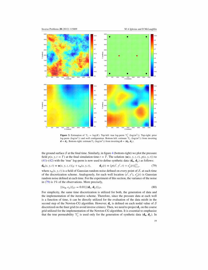
log-perm (log(m2)) and well configuration. Bottom-left: estimate )2 (log(m2)) from invertingd = dp. Bottom-right: estimate)2 (log(m2)) from inverting d = (du, dp).
the ground surface S at the final time. Similarly, in figure 4 (bottom-right) we plot the pressurefield p(x, y, t = T ) at the final simulation time t = T . The solution (u(x, y, z, t), p(x, y, t)) to(41)–(42) with the ‘true’ log-perm is now used to define synthetic data (du, dp) as follows:
du(x, y, t) ) u(x, y, z, t)|S + 2u(x, y, t), dp(t) ) {p(xl, yl, t) + 2lp(t)}13
l=1, (79)
where 2u(x, y, t) is a field of Gaussian random noise defined on every point of S, at each timeof the discretization scheme. Analogously, for each well location (xl, yl ), 2l
p(t) is Gaussianrandom noise defined at each time. For the experiment of this section, the variance of the noisein (79) is 1% of the observations. More precisely,
||(2u, 2p)||O = 0.01||(du, dp)||O. (80)
For simplicity, the same time discretization is utilized for both, the generation of data andthe implementation of the iterative scheme. Therefore, since the pressure data at each wellis a function of time, it can be directly utilized for the evaluation of the data misfit in thesecond step of the Newton-CG algorithm. However, du is defined on each nodal value of Sdiscretized on the finer grid (to avoid inverse crimes). Then, we need to project du on the coarsegrid utilized for the implementation of the Newton-CG algorithm. It is essential to emphasizethat the true permeability )†
2 is used only for the generation of synthetic data (du, dp). In
19
Inverse Problems 28 (2012) 115009 M A Iglesias and D McLaughlin
0 500 1000 1500 2000 2500 3000 3500 40000
500
1000
1500
2000
2500
3000
3500
4000
X (meters)
Y (
met
ers)
!0.1
!0.05
0
0.05
0.1
0.15
0 500 1000 1500 2000 2500 3000 3500 40000
500
1000
1500
2000
2500
3000
3500
4000
X (meters)
Y (
met
ers)
!0.15
!0.1
!0.05
0
0.05
0.1
0.15
0.2
0.25
0 500 1000 1500 2000 2500 3000 3500 40000
500
1000
1500
2000
2500
3000
3500
4000
X (meters)
Y (
met
ers)
!0.7
!0.6
!0.5
!0.4
!0.3
!0.2
!0.1
0
0.1
0.2
0 500 1000 1500 2000 2500 3000 3500 40000
500
1000
1500
2000
2500
3000
3500
4000
X (meters)
Y (
met
ers)
1.8
2
2.2
2.4
2.6
2.8
3
3.2
Figure 4. Solution to (41)–(42) for )2 = )†2 (i.e. ‘true’ log permeability). Top-left: ux(x, t = T )|S
(m). Top-right: uy(x, t = T )|S (m). Bottom-left: uz(x, t = T )|S (m). Bottom-right: p(x, y, t = T )('107 Pa).
addition, the covariance expression that we used for the generation of )†2 , is also utilized for
the definition of the space (28) (for i = 2). One can therefore think the covariance model asprior information incorporated into the inverse model. These prior information and syntheticdata are used in our Newton-CG scheme to find an estimate )2 of the log-permeability of thereservoir.
The experiment we present in this section (i.e. estimation of )2 = log(K) assuming )1
known) is motivated by the interest of the reservoir modeling community in finding estimatesof absolute permeability for improving the prediction of reservoir dynamics. However, most ofthe literature is focused on the estimation of permeability by inverting (or assimilation of) onlyproduction data from wells. In the present formulation, the assimilation of only production(pressure) data can be easily obtained by eliminating the second component of d = (du, dp),and setting -u ! * in (50). Thus, in this first set of experiments, we use our inversionapproach to compute an estimate of log-permeability when we invert only pressure data (i.e.we use d = dp). This estimate is shown in figure 3 (bottom-left). The same inversion approachis used to compute an estimate of log-perm when combined pressure and surface deformationdata are inverted (i.e. when we use d = (du, dp)). In this case, the estimate is displayed infigure 3 (bottom-right). We recall that for this experiment, )1 is known and so for simplicity we
20
Inverse Problems 28 (2012) 115009 M A Iglesias and D McLaughlin
5 10 15 20 25 30 35 40 45 50 55 60
1
1.5
2
2.5
3
3.5
4
Iteration number
log 10
[dat
a m
isfit
]2
inversion of d=d
pinversion of d=(d
p,d
u)
0 10 20 30 40 50 60160
162
164
166
168
170
172
174
Iteration number
|| !2!!
2* ||2
inversion of d=d
pinversion of d=(d
p,d
u)
0 20 40 60 80 100 120 140160
162
164
166
168
170
172
174
Iteration number
||!2!!
2* ||2
inversion of d=(d
p,d
u)
Figure 5. Performance of the procedure for the estimation of )2 = log(K). Top-left: log10 of thesquared data misfit. Top-right: squared error (expression (81)). The red solid line corresponds tothe case where only pressure data are inverted. The dotted black line indicates the performancewhen pressure and surface deformation data are inverted. Bottom: same experiment correspondingto the dotted line of the top-right panel. In this case, however, the discrepancy principle is notenforced.
choose )1(x, y) = 19.8 log (Pa) for all (x, y) " !1. In both cases, we initialize the Newton-CGalgorithm with the constant field shown in figure 3 (top-right). It comes as no surprise that theestimate computed by inverting only pressure data (from wells) recovers spatial features ofthe ‘true’ log-permeability )†
2 at the regions close to the well locations (figure 3 (top-right)).From figure 3 (bottom-right), we can visually appreciate that the estimate computed with bothpressure data and surface deformation has a better resemblance to )†
2 in regions in-betweenthe well locations. The performance of the estimation and the added value of the inversion ofsurface deformation is quantified with the errors defined by
E2()2) = ||)2 # )†2 ||K2 . (81)
In figure 5 (top-right), we display the errors (81) as a function of iterations of the Newton-CGscheme. We clearly observe that the error with respect to the true log-permeability )†
2 is smallerwhen both pressure and surface deformation are inverted. In both cases, we see that the datamisfit, presented in figure 5 (top-left), decreases with the number of iterations. The Newton-CG scheme is stopped according to the discrepancy principle (61) with 1 = 2.5. In figure 5(bottom), we display again the error when both types of data are inverted. However, in this casethe Newton-CG scheme is not stopped according to the discrepancy principle. We then note
21
Inverse Problems 28 (2012) 115009 M A Iglesias and D McLaughlin
an increase of the error after it reaches a minimum. This constitutes the numerical evidence ofthe ill-posedness predicted by corollary 3.1 due to the compactness of the forward operator.In other words, even though the current estimate predicts data close to the observations (inthe observation space), the corresponding estimate diverges (in the parameter space) from thetrue log-permeability )†
2 .
4.2.2. Estimation of )1 = log("). In this section, we assume that )2 = log(K) is known.For simplicity, we consider a constant field )2(x, y) = #27.6 log(m2) for all (x, y) " !2.The goal is now to test the inversion approach for finding an estimate )1 = log(") fromsynthetic data. Since " is an elastic property, it is clear that data from surface deformation aremore sensitive to changes in ". Conversely, there is a low sensitivity in the pressure data withrespect to ". Due to this low sensitivity, very poor estimates (not shown) of " are obtainedwhen only pressure data are inverted. Therefore, for this experiment we consider the inversionof combined synthetic surface deformation and pressure data.
For the generation of synthetic data, we define a ‘true’ elastic parameter )1 = log(")
statistically generated with sequential Gaussian simulation. We used a spherical covariancemodel with horizontal range of 3 km and vertical range of 1 km. The generated Gaussian fieldis denoted by )†
1 and presented in figure 6 (top). We recall that the elastic property )†1 must
be defined in !1. For reference, in figure 7 (top-left) we display the values of )†1 at !2, i.e.
22
Inverse Problems 28 (2012) 115009 M A Iglesias and D McLaughlin
)†1 (x, y, z = 300 m). The ‘true’ log-lambda is then used to solve the model equations (41)–
(42). Then, synthetic data are generated by adding noise of 1% as described in the previousexperiment. The initial guess for algorithm 1 is a constant field )1(x, y) = 19.8 log(m2) for all(x, y) " !1. In figure 6, (bottom) we present the estimate )1 obtained after 80 iterations of theiterative scheme. After this number of iterations, the data misfit displayed in figure 7 (bottom)exhibits stagnation around a value that satisfies the discrepancy principle with 1 = 3.6.The corresponding values of the estimate at the reservoir )1(x, y, z = 300 m) are shown infigure 7 (top-right). There is a clear visual agreement between the truth and the estimate. Thisagreement can be quantified by means of the error
E1()1) = ||)1 # )†1 ||K1 . (82)
The square of this error as well as the performance of the squared data misfit is displayedin figure 7 (bottom). It is worth mentioning that the main agreement between )†
1 and )1 should
23
Inverse Problems 28 (2012) 115009 M A Iglesias and D McLaughlin
be expected at the reservoir !2. This can be easily understood by recalling that the only sourcefor the elastic deformation of !1 is the subsurface flow which is considered only within thereservoir !2. It is therefore not surprising that the estimate )1 does not capture all the spatialfeatures of )†
1 . Nevertheless, in the norm of the parameter space K1 (defined in !1), the errorof the estimate )1 decreases with the number of iterations (see figure 7 (bottom)).
4.2.3. Multiple-parameter estimation. We now present a final experiment where we test thecapability of the Newton-CG algorithm to find joint estimates of )1 and )2 from combinedsynthetic pressure data and surface deformation (i.e. d = (du, dp)). In this experiment, weshow the effect of the noise level on the estimation. Additionally, we numerically expose anapparent increase of the ill-posedness, in the sense of uniqueness, of the IP. Since the parameters)1 = log(K) and )2 = log(") are spatially varying functions, the lack of uniqueness is alsoexperienced in the case of single-parameter estimation. In fact, nonuniqueness was observedin the experiments presented in sections 4.2.1 and 4.2.2. Indeed, both estimates and the truthare, within the noise level, solutions to the IP. Nevertheless, we are interested in recovering,at least partially, spatial features from the true properties. Intuitively, in the multiparameterestimation, one expects that ‘many more’ possible combinations of functions ()1,)2) can leadto the same data d = (du, dp). In the experiment below, we show that completely inaccurateestimates can be obtained for large measurement errors.
The true log-perm )†2 and ‘true’ log-lambda )†
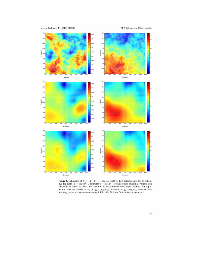
1 are the fields displayed in figures 8(top-left) and 9 (top), respectively. Synthetic data are generated with the same procedure asbefore. However, for this experiment we generated four sets of synthetic data correspondingto noise levels of 1%, 10%, 20% and 30% of the measurements. For all those sets, the CGalgorithm is initialized with constant fields with values )1(x, y) = 19.8 log(m2) ((x, y) " !1)and )2(x, y) = #27.6 log(m2) ((x, y) " !2). For each set of data, the corresponding estimates()1,)2) from the iterative scheme are presented from the second to fifth row of figures 8 and9. In the second column of figure 8 we additionally present the restriction of )1 to !2 (thereservoir). The misfit between data and model predictions is displayed in figure 10 (left). Theerror of the estimates with respect to the truth is presented in figure 10 (right). The previousgraph quantifies the detrimental effect of noise in the observations. In this case, the visualappreciation can be misleading. For example, one may argue that the permeability estimateobtained from data contaminated with 20% error provides a visually better estimate than theestimates obtained with smaller errors. However, in the joint estimation, one should expect adecrease in the total error which includes also the estimate of log-lambda. More precisely, thesquared error in figure 10 (right) is defined by
E ()1,)2)2 = E1()1)
2 + E2()2)2 (83)
with E1 and E2 as defined in (82) and (81), respectively. It is also interesting to observe, fromfigure 10 (left), that the data misfit decreases and stagnates at a value which satisfies thediscrepancy principle for 1 = 2.6 (1%), 1 = 0.975 (10%), 1 = 0.98 (20%), and 1 = 0.97(30%). Similar values of 1 were also found in [17, 18], where iterative regularization techniqueswere applied to parameter identification in reservoir models [17, 18]. Moreover, as indicatedin [15], it is possible to obtain decrease of the error for 1 s smaller than the ones predicted bythe theory (see corollary 3.1).
We now compare the performance of the Newton-CG scheme for producing estimatesin the case of multiparameter estimation against the single-parameter estimation case of theprevious subsections. We emphasize that those single-parameter estimation examples differsubstantially from multiparameter estimation. In other words, they are all different inverseproblems. The aim here is to show the suboptimal performance of the multiparameter case. To
24
Inverse Problems 28 (2012) 115009 M A Iglesias and D McLaughlin
0 500 1000 1500 2000 2500 3000 3500 40000
500
1000
1500
2000
2500
3000
3500
4000
X (meters)
Y (
met
ers)
!30
!29.5
!29
!28.5
!28
!27.5
!27
!26.5
!26
!25.5
0 500 1000 1500 2000 2500 3000 3500 40000
500
1000
1500
2000
2500
3000
3500
4000
X(meters)
Y(m
eter
s)
18
18.5
19
19.5
20
20.5
21
21.5
22
0 500 1000 1500 2000 2500 3000 3500 40000
500
1000
1500
2000
2500
3000
3500
4000
X(meters)
Y(m
eter
s)
!29.5
!29
!28.5
!28
!27.5
!27
!26.5
!26
!25.5
0 500 1000 1500 2000 2500 3000 3500 40000
500
1000
1500
2000
2500
3000
3500
4000
X(meters)
Y(m
eter
s)
18
18.5
19
19.5
20
20.5
21
21.5
22
0 500 1000 1500 2000 2500 3000 3500 40000
500
1000
1500
2000
2500
3000
3500
4000
X(meters)
Y(m
eter
s)
!29.5
!29
!28.5
!28
!27.5
!27
!26.5
!26
!25.5
0 500 1000 1500 2000 2500 3000 3500 40000
500
1000
1500
2000
2500
3000
3500
4000
X(meters)
Y(m
eter
s)
18
18.5
19
19.5
20
20.5
21
21.5
22
Figure 8. Estimation of ! = ()1,)2) = (log("), log(K)). Left column, from top to bottom:true log-perm ()/
2 ) (log(m2)), estimates )2 (log(m2)) obtained from inverting synthetic datacontaminated with 1%, 10%, 20% and 30% of measurement error. Right column, from top tobottom: true log-lambda in !2 ()/
1 |!2 ) (log(Pa)), estimates )1|!2 (log(Pa)) obtained frominverting synthetic data contaminated with 1%, 10%, 20% and 30% of measurement error.
25
Inverse Problems 28 (2012) 115009 M A Iglesias and D McLaughlin
0 500 1000 1500 2000 2500 3000 3500 40000
500
1000
1500
2000
2500
3000
3500
4000
X(meters)
Y(m
eter
s)
!29.5
!29
!28.5
!28
!27.5
!27
!26.5
!26
!25.5
0 500 1000 1500 2000 2500 3000 3500 40000
500
1000
1500
2000
2500
3000
3500
4000
X(meters)
Y(m
eter
s)
18
18.5
19
19.5
20
20.5
21
21.5
22
0 500 1000 1500 2000 2500 3000 3500 40000
500
1000
1500
2000
2500
3000
3500
4000
X(meters)
Y(m
eter
s)
!29.5
!29
!28.5
!28
!27.5
!27
!26.5
!26
!25.5
0 500 1000 1500 2000 2500 3000 3500 40000
500
1000
1500
2000
2500
3000
3500
4000
X(meters)
Y(m
eter
s)
18
18.5
19
19.5
20
20.5
21
21.5
22
Figure 8. (Continued.)
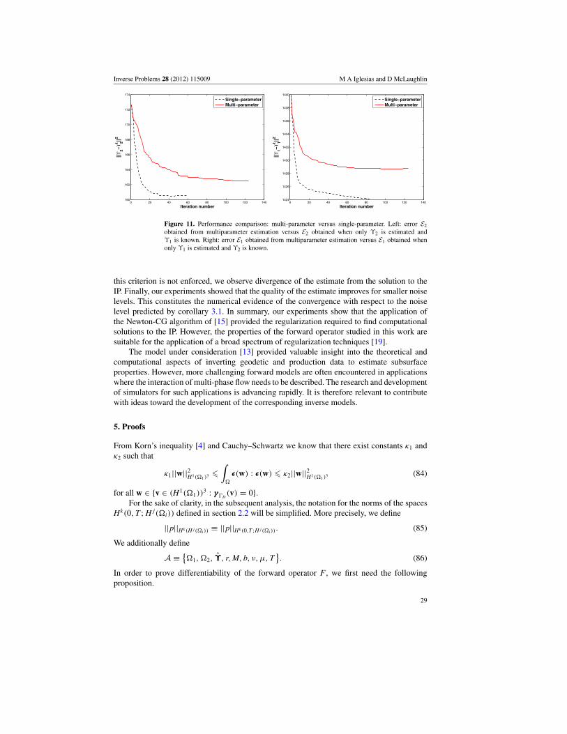
the left (respectively right) of figure 11 we display the comparison in the norm (81) (respectively(82)) when multiparameter estimation is compared to single parameter-estimation for log(K)
(respectively log(")). Both, visually and quantitatively, the multiparameter estimate providessuboptimal results with respect to the single-parameter estimation case.
We finally remark that, for the multi-parameter case, the estimation of both parametersdepends on the relative magnitudes of the norms in (32) (recall + = 1 for this experiment).Then, by modifying + in (32), more weight can be given to one or the other parameter based onthe prior knowledge of the subsurface properties. To the best of our knowledge, in the contextof inverting properties in geomechanics-flow model, the optimal choice of the weighting factorbetween the two subsurface properties is an open problem.
4.3. Conclusions and future work
Our synthetic experiments suggest that elastic and rock properties of the subsurface can beestimated via data inversion of coupled flow-geomechanics models. In the single-parameterestimation case, when both surface deformation and pressure data are inverted, more accurateestimates of permeability were obtained with respect to the ones obtained from onlyinverting pressure data. Furthermore, reasonable estimates of one of the elastic moduli wereaccomplished in the single-parameter case. In the multi-parameter case, suboptimal jointestimates of log(K) and log(") were obtained with respect to the single-parameter estimates.
26
Inverse Problems 28 (2012) 115009 M A Iglesias and D McLaughlin
0
1000
2000
3000
4000
0
1000
2000
3000
40000
100
200
300
400
500
600
700
18
18.5
19
19.5
20
20.5
21
21.5
22
0
1000
2000
3000
4000
0
1000
2000
3000
40000
100
200
300
400
500
600
700
18
18.5
19
19.5
20
20.5
21
21.5
22
0
1000
2000
3000
4000
0
1000
2000
3000
40000
100
200
300
400
500
600
700
18
18.5
19
19.5
20
20.5
21
21.5
22
Figure 9. Estimation of ! = ()1,)2) = (log("), log(K)). From top to bottom: true log-lambda)/
1 (log(Pa)), and estimates )1 (log(Pa)) obtained from inverting synthetic data contaminatedwith 1%, 10%, 20% and 30% of measurement error.
Nevertheless, those suboptimal estimates displayed some of the spatial features of the trueproperties. The lack of accuracy of the estimates in the multi-parameter case was presumablyassociated with the increase of ill-posedness (non-uniqueness) with respect to the single-parameter case.
27
Inverse Problems 28 (2012) 115009 M A Iglesias and D McLaughlin
0
1000
2000
3000
4000
0
1000
2000
3000
40000
100
200
300
400
500
600
700
18
18.5
19
19.5
20
20.5
21
21.5
22
0
1000
2000
3000
4000
0
1000
2000
3000
40000
100
200
300
400
500
600
700
18
18.5
19
19.5
20
20.5
21
21.5
22
Figure 9. (Continued.)
0 20 40 60 80 100 120 1405
6
7
8
9
10
11
12
Iteration number
log 10
[dat
a m
isfit
]2
1%10%20%30%
0 20 40 60 80 100 120 1401590
1595
1600
1605
1610
1615
Iteration number
||!1!!
1t ||2 +||!
2!!2t ||2
1%10%20%30%
Figure 10. Performance of the estimation of ! = ()1,)2) = (log("), log(K)) for different noiselevels. Left: log10 squared data misfit. Right: error.
As we expect from the theoretical results of section 3, the utilized Newton-CG algorithmprovided stable computational solutions of the IP. More precisely, the stopping criteria(discrepancy principle) of the scheme ensured that the decrease of the data misfit correspondedto a decrease in the error of the estimate with respect to the solution to the IP. Moreover, when
28
Inverse Problems 28 (2012) 115009 M A Iglesias and D McLaughlin
0 20 40 60 80 100 120 140160
162
164
166
168
170
172
174
Iteration number
||!2!!
2t ||2
Single!parameterMulti!parameter
0 20 40 60 80 100 120 1401424
1426
1428
1430
1432
1434
1436
1438
1440
Iteration number
||!1!!
1t ||2
Single!parameterMulti!parameter
Figure 11. Performance comparison: multi-parameter versus single-parameter. Left: error E2obtained from multiparameter estimation versus E2 obtained when only )2 is estimated and)1 is known. Right: error E1 obtained from multiparameter estimation versus E1 obtained whenonly )1 is estimated and )2 is known.
this criterion is not enforced, we observe divergence of the estimate from the solution to theIP. Finally, our experiments showed that the quality of the estimate improves for smaller noiselevels. This constitutes the numerical evidence of the convergence with respect to the noiselevel predicted by corollary 3.1. In summary, our experiments show that the application ofthe Newton-CG algorithm of [15] provided the regularization required to find computationalsolutions to the IP. However, the properties of the forward operator studied in this work aresuitable for the application of a broad spectrum of regularization techniques [19].
The model under consideration [13] provided valuable insight into the theoretical andcomputational aspects of inverting geodetic and production data to estimate subsurfaceproperties. However, more challenging forward models are often encountered in applicationswhere the interaction of multi-phase flow needs to be described. The research and developmentof simulators for such applications is advancing rapidly. It is therefore relevant to contributewith ideas toward the development of the corresponding inverse models.
5. Proofs
From Korn’s inequality [4] and Cauchy–Schwartz we know that there exist constants +1 and+2 such that
+1||w||2H1(!1)3 !,
!
"(w) : "(w) ! +2||w||2H1(!1)3 (84)
for all w " {v " (H1(!1))3 : $%D
(v) = 0}.For the sake of clarity, in the subsequent analysis, the notation for the norms of the spaces
Hk(0, T ; H j(!i)) defined in section 2.2 will be simplified. More precisely, we define
||p||Hk(H j (!i )) ) ||p||Hk(0,T ;H j (!i)). (85)
We additionally define
A ).!1,!2, !, r, M, b, #, µ, T
/. (86)
In order to prove differentiability of the forward operator F , we first need the followingproposition.
29
Inverse Problems 28 (2012) 115009 M A Iglesias and D McLaughlin
5.1. Proof of proposition 2.1
Let ! " K and r > 0. Let ! = ()1,)2) " B(!, r) and consider (43)–(44). The existenceand uniqueness of h(!) ) (u, p) " H1(0, T ; H0)' (H1(0, T ; L2(!2))%L*(0, T ; H1(!2)))
that solves (43)–(44) follows directly from [13, theorem 2.1]. Note that "(x) = e)1(x) > 0 forall x " !1, and (from our choice) " " K1 ,! C(!). Then, coercivity and continuity of thebilinear form (43) can be established from standard arguments as for the case of constant " of[13]. In addition, from our selection )2 " K2, the embedding K2 ,! C1(!2) and the fact thatu " H1(0, T ; H0), it follows from [24] that p " H2,1(!2 ' [0, T ]), where [24]
H2,1(!2 ' [0, T ]) ) L2(0, T ; H2(!2)) % H1(0, T ; L2(!2)) (87)
with norm (24). Additionally, it can be shown [17, corollary 3.1] that
where C may depend only on !2, !, T and r. In other words, estimate (88) holds uniformlyin B(!, r).
The following proof consists of using the variational formulation (43)–(44) to find errorestimates for p and u that will lead to (45). Let us take (w, w) =
'$u$t , p
)in (43)–(44) to find
12
ddt
,
!1
e)1 ($ · u)2 + 12
ddt
,
!1
µ"(u) : "(u) #,
!2
bp$ · $u$t
=,
!1
f1 · $u$t
+,
!1
f2$ · $u$t
, (89)
1M
12
ddt
,
!2
p2 +,
!2
##1 e)2 |$p|2 +,
!2
b$($ · u)
$tp =
,
!2
f3 p. (90)
We integrate the previous expressions from 0 to t and integrate by parts (with respect totime) the right-hand side of (89). We additionally use that u(·, 0) = 0 and add the resultingexpressions to arrive at
We combine (95) with (88) and (97) to finalize the proof .
5.2. Proof of theorem 2.1
Consider the following observation.
Observation 1. It is straightforward to show that the exponential operators e)1 : C(!) !C(!) and e)2 : C1(!2) ! C1(!2) are continuously Frechet differentiable. From the assumedembedding K1 ,! C(!) and K2 ,! C1(!2), it follows easily that e)1 : K1 ! C(!1) ande)2 : K2 ! C1(!2) are also continuously Frechet differentiable.
We now prove the following lemma.
Lemma 5.1. Let G : K ! H be the mapping G(!) = h ) (u, p) given by the solution to thevariational model (41)–(42). G is continuous in K.
Proof. Let ! " K and 2 > 0. Let h = (u, p) as above. Let C > 0 be the constant granted byproposition 2.1 applied to B(!, 1). Define
A ) C2(1 + 2##1)(||p0||H1(!2) + ||q||L2(L2(!2)) + ||f||H1(L2(!1))). (98)
32
Inverse Problems 28 (2012) 115009 M A Iglesias and D McLaughlin
From observation 1, we take * > 0 such that
||e)1 # e)1 ||C(!1) + ||e)2 # e)2 ||C1(!2) ! 2
A, (99)
provided that
||)1 # )1||K1 + ||)2 # )2||K2 < *. (100)
Let * ) min{1, *}. Proposition 2.1 ensures that for every ! " K with ||! # !||K ! *,
where h(!) = (u, p) is the solution to (41)–(42) for !. Moreover, from (41)–(42) it is notdifficult to see that h # h satisfies
L()1, u # u, w) #,
!2
b[p # p]$ · w =,
!1
3(e)1 # e)1 )($ · u)($ · w), (102)
,
!2
1M
$[p # p]$t
w +,
!2
##1e)2$ · [p # p] · $w +,
!2
b$$ · [u # u]
$tw
= #,
!2
##1w$ · (e)2 # e)2 )$ p, (103)
for all (w, w) " W . The right-hand side of (103) has been obtained after integrating by partsand using the boundary condition (9). Proposition 2.1 can be now applied to (102)–(103).Therefore,
Note that, from proposition 2.1, the constant C in (104) (and therefore in (106)) is the same asin (101). We finally combined (106) with (98), (99) and (101) to obtain
||h # h||H ! C2
A(1 + 2##1)||h||H ! 2, (107)
which proves the continuity of G at an arbitrary ! " K . "For )i, )i " Ki (i " {1, 2}). Let us define the residuals
R()i, )i) ) e)i # e)i # ()i # )i) e)i . (108)
Lemma 5.2. Let !, ! " K and h(!) = (u, p), h(!) = (u, p) be the corresponding solutionsto (41)–(42). Let % = (%u, 3p) be the solution to
L1()1, %u, w) #,
!2
b3p$ · w +,
!1
()1 # )1) e)1 ($ · u)($ · w) = 0, (109)
,
!2
1M
$3p
$tw +
,
!2
##1 e)2$3p · $w +,
!2
b$$ · %u
$tw
+,
!2
##1()2 # )2) e)2$p · $w = 0, (110)
33
Inverse Problems 28 (2012) 115009 M A Iglesias and D McLaughlin
for all (w, w) " W . Then, the residuals
ru ) u # u # %u, rp ) p # p # 3p, (111)
are the solutions to the following variational problem
L1()1, ru, w) #,
!2
brp$ · w = #,
!1
R()1, )1)($ · u)($ · w)
+,
!1
()1 # )1) e)1 ($ · (u # u))($ · w), (112)
,
!2
1M
$rp
$tw +
,
!2
##1 e)2$rp · $w +,
!2
b$$ · ru
$tw = #
,
!2
##1R()2, )2)$ p · $w
+,
!2
##1 e)2 ()2 # )2)($ p # $p) · $w, (113)
a.e. in (0, T ] for all (w, w) " W .
Proof. The proof is straightforward from (40), (41)–(42) and (53)–(54). "
Proof of theorem 2.1. Let ! " K be arbitrary but fixed and 2 > 0. Let h ) (u, p) be thesolution to (41)–(42) for all W " W a.e. t " (0, T ]. Let ! " K be arbitrary and let h ) (u, p)
be the corresponding solution to(41)–(42), for all W " H a.e. in (0, T ]. Let Ce and CS begiven by (33) and (19), respectively. Define
4 ) max{||e)2 ||C1(!2), ||e)1 ||C(!1)}, (114)
and
A )*
1-p
N+
j=1
||*(x # xl )||2L2(!2) dt + 1-u
CS
-1/2
C(2##1 + 1)(||h||H + Ce4). (115)
From the lemma 5.1, we take *1 > 0 such that
||h # h||H ! 2
A, (116)
provided ||! # !||K ! *1. Consider the residuals defined in (108). From observation 1 let*2 > 0 be such that
||R()1, )1)||C(!1) ! 2
A||[)1 # )1]||K1 (117)
||R()2, )2)||C1(!2) ! 2
A||[)2 # )2]||K2 , (118)
provided that ||)i # )i||Ki ! *2 (i = 1, 2). Let C > 0 be the constant from proposition 2.1applied to B(!, min{*1, *2}). Then,
provided ||! #!||K ! min{*1, *2}. Let % = (%u, 3p) be the solution to (109)–(110) that existsdue to proposition 2.1. We now show that DF(!)(! # !) = (Mu(%u),M(3p)). We firstdefine the residuals r = (ru, rp) (111), and note that
Inverse Problems 28 (2012) 115009 M A Iglesias and D McLaughlin
which from (46)–(50) becomes
||F(!) # F(!) # DF(!)(! # !)||2O = 1-p
, T
0|Mp(rp)|2dt + 1
-u
, T
0
,
S|$S (ru)|2 d- dt
! 1-p
, T
0||rp||2L2(!2)
N+
j=1
||*(x # xl )||2L2(!2 )dt + 1-u
, T
0CS ||ru||2H1(!1)dt
!*
1-p
N+
j=1
||*(x # xl )||2L2(!2 )dt + 1-u
CS
-||r||2H. (121)
The rest of the proof consist of finding a bound for ||r||2H so that the differentiability can beestablished. From lemma 5.2 we know that r = (ru, rp) satisfy (112)–(113). So, we integrateby parts the right-hand side of (113) and apply the boundary condition (9) to find,
!2
1M
$rp
$tw +
,
!2
##1 e)2$rp · $w +,
!2
b$($ · ru)
$tw =
,
!2
##1$ · (R()2, )2)$ p)w
#,
!2
##1$ · (e)2 ()2 # )2)($ p # $p))w. (122)
It is not difficult to see that (112) and (122) can be written as (43)–(44) for f1 = 0 and
Inverse Problems 28 (2012) 115009 M A Iglesias and D McLaughlin
5.3. Proof of theorem 3.1
Let B be a bounded set in K. We prove that F(B) is a relatively compact set in O. Note that
F(B) = {(Mu(u),Mp(p)) " O|h(!) = (u, p)is the solution to (41)–(42) for! " B}.Therefore, F(B) = F1(B) ' F2(B) where
F1(B) = {Mu(u) " L2(0; T, L2(S )3)|u is the first component of h(!) = (u, p) with! " B},F2(B) = {Mp(p) " L2[0; T ]N |p is the second component of h(!) = (u, p) with! " B}.We first prove that F2 is relatively compact in L2(0; T, L2(S )3). We do so by verifying that thehypotheses of [31, theorem 1] are satisfied. In other words, we show that
(1) {9 t2
t13 (t) dt : 3 " F2(B)} is relatively compact in L2(S )3 for all 0 < t1 ! t2 < T .
(2) ||3 (t + h) # 3 (t)||L2(0,T#h;L2(S )3) ! 0 as h ! 0 uniformly in F2(B).
To show (1), we consider an arbitrary sequence in. 9 t2
t13 (t) dt : 3 " F2(B)
/. In other
words, we consider: , t2
t1Mu(un(t))dt : un is the first component of h(!n) = (u, p) with !n " B
;
, (130)
for an arbitrary sequence !n " B. Then, ||!n||K ! C1 for all n " N. From proposition 2.1and (45), it follows that
for all t " [0, T ] and for some constant C > 0 that depends on T . Then, (132) implies thatthe sequence ||un(·, t)||H1(!1)3 is bounded for all t " [0, T ]. Since the trace $S : H1(!1)
3 !L2(S )3 is a compact operator [22, theorem 6.10.5], there exists a subsequence also denotedby $S (un(·, t)) and +/
t " L2(S )3 such that
$S (un(·, t)) ! +/t strongly in L2(S )3, (133)
as n ! *, for all t " [0, T ]. Let us define + : [0, T ] ! L2(S )3 by +(t) ) +/t . Since + is the
pointwise limit of strongly measurable functions, + itself is strongly measurable [16, theorem3.5.4(3)]. We then have that
||$S (un(·, t)) # +(t)||L2(S )3 ! 0, (134)
for every t " [0, T ]. In addition, from (19) and (132) we know that
||$S (un(t))||L2(S ) ! CSCQ,
which after passing the limit yields,
||+(t)||L2(S ) ! CSCQ.
From the two previous estimates we obtain
||$S (un(·, t)) # +(t)||L2(S )3 ! 2CSCQ, (135)
for all t " [0, T ] and for all n " N. Let t1, t2 " (0, T ) such that t1 ! t2. Define gn : R ! R by
gn(t) ):
([t1,t2]||$S (un(·, t)) # +(t)||L2(S )3 t " [0, T ]
0 t /" [0, T ],(136)
36
Inverse Problems 28 (2012) 115009 M A Iglesias and D McLaughlin
where ([t1,t2] is the characteristic function of [t1, t2]. Then, from (135) and (134) we observethat
|gn(t)| ! 2CSCB, limn!*
gn(t) = 0, (137)
for all t " R. Then, from the dominated convergence theorem [8, theorem 2, 5.9.2], it followsthat
limn!*
, t2
t1||$S (un(·, t)) # +(t)||L2(S )3 = lim
n!*
,
Rgn(t) dt =
,
Rlim
n!*gn(t) dt = 0. (138)
On the other hand, from [8, theorem 8, E.5],((((((, t2
t1($S (un(·, t)) # +(t)) dt
((((((L2(S )3
!, t2
t1||$S (un(·, t)) # +(t)||L2(S )3 dt,
which combined with (138) yields,, t2
t1Mu(un(t)) dt )
, t2
t1$S (un(t)) dt !
, t2
t1+(t) dt in L2(S )3, (139)
for arbitrary 0 < t1 ! t2 < T . We have shown that an arbitrary sequence. 9 t2
t1Mu(un(t)) dt
/
has a convergent subsequence for all 0 < t1 ! t2 < T . Then, the set. 9 t2
t13 (t) dt : 3 " F2(B)
/
is relatively compact in L2(S )3 for all 0 < t1 ! t2 < T which proves (1). On the other hand,from [8, theorem 2, 5.9.2] we have that
un(t + h) # un(t) =, t+h
t
dun
dtdt, (140)
for all h > 0. Then, for all t " [0, T # h], [8, theorem 8, E.5] and Cauchy–Schwarz yield
which implies ||$(un(t + h)) # $(un(t))||L2(0,T#h;L2(S )) ! 0 as h ! 0 for all n " N whichestablishes (2). Then F2(B) is relatively compact in L2(0, T ; L2(S )3).
To prove that F1(B) is relatively compact in L2[0, T ]N , we take a sequence !n " B. Fromthe same argument as before, we have
where C depends on C1. Then pn is a bounded sequence in H2,1(!2 ' [0, T ]). From theLions–Aubin theorem [30, proposition III, 1.3] we know that H2,1(!2 ' [0, T ]) is compactlyimbedded in L2(0, T ; L2(!2)). Therefore, for some subsequence (also denoted by pn) wehave that pn ! p/ (strongly) in L2(0, T ; L2(!2)) for some p/ " L2(0, T ; L2(!2)). From thecontinuity of Mp it follows that
Mp(pn) ! Mp(p/) strongly in L2(0, T )N, (143)
which proves that F1(B) is relatively compact in L2(0, T )N . Since F1(B) and F2(B) arerelatively compact in L2(0, T ; L2(S )3) and L2(0, T )N , respectively, then F(B) is relativelycompact in O which establishes the compactness of F .
We now prove that F is weakly sequentially closed. Let us take an arbitrary sequence!n 5 ! " K. Let us assume that F(!n) 5 (yu, yp) in O. First we note that theembeddings in (33) are compact. Then, there exist ! ) ()1,)2) " C(!1) ' C1(!2) such
37
Inverse Problems 28 (2012) 115009 M A Iglesias and D McLaughlin
that )n1 ! )1 strongly in C(!1) and )n
2 ! )2 strongly in C1(!2). Let hn(!n) ) (un, pn)
and h(!) ) (u, p) be the solutions to (41)–(42) for !n and !, respectively. It is not difficultto see that hn # h = (un # u, pn # p) satisfies
L()n1 , un # u), w) #
,
!2
b[pn # p]$ · w =,
!1
[(e)1 # e)n1 )($ · u)($ · w), (144)
,
!2
1M
$[pn # p]$t
w +,
!2
##1 e)n2 $ · [pn # p] · $w +
,
!2
b$$ · [un # u]
$tw,
= #,
!2
##1w$ · (e)2 # e)n2 )$p (145)
for all (w, w) " W . We now prove that hn ! h " H. Let 2 > 0. From continuity of theexponential function, let * > 0 such that
||e)1 # e)1 ||C(!1) ! 2
A, ||e)2 # e)2 ||C1(!2) ! 2
A, (146)
with
A ) C#1(||u||H1(H1(!1)) + 2##1||p||L2(H2(!2)))#1, (147)
provided that ||)1 # )1||C(!1) ! * and ||)2 # )2||C1(!2) ! *. Let N " N such that||)n
1 # )1||C(!1) ! * and ||)n2 # )2||C1(!2) ! * for every n # N. From proposition 2.1
which implies that hn ! h " H. From the continuity of Mp and Mu, it follows thatF(!n) ! F(!) (strongly) in O. Therefore, F(!n) 5 F(!). From uniqueness of the limitof a weak convergent sequence, we find F(!) = (yu, yp) which proves that F is weakly(sequentially) closed.
5.4. Proof of theorem 3.2
The proof of 3.2 requires the following analysis. For i " {1, 2} we define
!>i ) {x " !i : |)i # )i| > 0} (150)
and
W ()i,)i) =
<=>
=?
R()i, )i)
e)i # e)1if x " !>
i
0 if x " ! # !>i
(151)
where the residuals are defined in (108) The following proposition is needed.
Lemma 5.3. For all !, ! " K, W ()1,)1) " L*(!1), W ()2,)2) " W 1,*(!2).Additionally, for every ! " K, there exists r > 0 such that for all !, ! " B(!, r)
||W ()1,)1)||L*(!1) ! C||)1 # )1||C(!1) (152)
||W ()2,)2)||H1(!2) ! C||)2 # )2||C1(!2) (153)
where C may depend only on !1, !2, ! and r.
38
Inverse Problems 28 (2012) 115009 M A Iglesias and D McLaughlin
Proof. The proof is very similar to the one of proposition 3.1 in [17] and so we omit it. "
Lemma 5.4. For every ! " K, there exists r > 0 such that for all !, ! " B(!, r) and all(vu, vp) " L2(0, T ; L2(!1))'H2,1(!2 ' [0, T ]) there exist functions .u " L2(0, T ; H0(!1))
Proof. For almost every t in [0, T ], let 6(·, t) be the solution to the following problem:
$ · $6(·, t) = W ()1,)1)vu in !1, (158)
6(·, t) = 0 on $!1, (159)
The existence of a unique solution 6(·, t) " H1(!1) to (158)–(159) follows from standardPDE theory. Furthermore, from elliptic regularity we know that 6(·, t) " H2(!1) and
||6(·, t)||H2(!1) ! C||W ()1,)1)vu||L2(!1), (160)
where C may possibly depend on !1. Similar arguments to the ones used in the proof oflemma 3.3 in [17] can be applied here to show that 6 : [0, T ] ! H2(!1) is stronglymeasurable. Then, from (160) and the previous proposition, it follows easily that 6 "L2(0, T ; H2(!1)). We define .u ) $6 " L2(0, T ; H1(!1)
3) and note that (158) impliesthat .u satisfies (154) a.e. in [0, T ]. Moreover, from (160)
which from the previous proposition implies (156). The existence of .p in (155) and estimate(157) follows directly from lemma 3.3 in [17]. "
Proof of theorem 3.2. Let r > 0 be such that the results of lemma 5.4 and assumption 3.1hold on B(!, r). Let C > 0 be the maximum of the corresponding Cs in (156)–(157) and(69)–(70). Let !, ! " B(!, r). Let % = (%u, 3p) be the solution to (109)–(110) which existfrom proposition 2.1. Let r = (ru, rp) be the residuals defined as in (111) of lemma 5.2. Notethat, in terms of these residuals, the left-hand side of (71) can be written as
||F(!) # F(!) # DF(!)(! # !)||2O = 1-p
, T
0|Mp(rp)|2 dt + 1
-u
, T
0
,
S|Mu(ru)|2.
(162)
39
Inverse Problems 28 (2012) 115009 M A Iglesias and D McLaughlin
From lemma 5.2, r = (ru, rp) satisfies (112)–(113) which after adding and using (151)becomes
L()1, ru, w) #,
!2
brp$ · w +,
!2
1M
$rp
$tw +
,
!2
b$$ · ru
$tw +
,
!2
##1 e)2$rp · $w
= #,
!1
W ()1,)1)(e)1 # e)1 )($ · u)($ · w)
+,
!1
()1 # )1) e)1'$ · (u # u)
)($ · w)
#,
!2
##1W ()2,)2)(e)2 # e)2 )$ p · $w
+,
!2
(##1 e)2 ()2 # )2)$(p # p) · $w)
for all (w, w) " W . In particular, the previous expression holds (a.e. in (0, T )) for(w, w) ) (w j
u(·, t), w jp(·, t)) where W = (w j
u(x, t), w jp(x, t)) is the solution to the adjoint
problem (72)–(73) with
A1 ) 1N-u
$S (ru), Aj2 ) 1
-p*(x # x j)
,
!2
rp(3 , t)*(3 # x j) d3 , (163)
for some j " {1, . . . , N}. Therefore,, T
0L()1, ru, w j
u) #, T
0
,
!2
brp$ · w ju +
, T
0
,
!2
1M
$rp
$tw j
p +, T
0
,
!2
b$$ · ru
$tw j
p
+, T
0
,
!2
##1 e)2$rp · $w jp =
, T
0(Dj
1 + Dj2) dt, (164)
where
Dj1 ) #
,
!1
(W ()1,)1)(e)1 # e)1 )($ · u)($ · w ju)
+,
!1
()1 # )1) e)1 ($ · (u # u))($ · w ju), (165)
Dj2 )
,
!2
##1W ()2,)2)(e)2 # e)2 )$ p · $w jp +
,
!2
(##1 e)2 ()2 # )2)$(p # p) · $w jp).
˜ (166)
On the other hand, since W = (w ju(x, t), w j
p(x, t)) satisfies (72)–(73) a.e. in (0, T ) for all(h1, h2) " W , in particular, for h1 = ru(·, t) and h2 = rp(·, t), (72)–(73) become
L()1, ru, w ju) #
,
!2
b$w
jp
$t$ · ru = 1
N-u
,
S|$S (ru)|2,
,
!2
*#brp$ · w j
u # rp1M
$wjp
$t# ##1 e)2$w j
p · $rp
-= 1
-p
* ,
!2
rp*(x # x j)
-2
.
We add the resulting equations, use (46), (48), integrate in (0, T ), integrate by parts some ofthe terms and use the fact that w
jp(·, T ) = ru(·, 0) = rp(·, 0) = 0 to find
, T
0L()1, ru, w j
u) +,
!2
b$$ · ru
$tw j
p
+, T
0
,
!2
5# brp$ · w j
u + w jp
1M
$rp
$t# ##1 e)2$w j
p · $rp
6
= 1-p
, T
0
'M j
p(rp))2 + 1
N-u
, T
0||Mu(ru)||2L2(S ).
40
Inverse Problems 28 (2012) 115009 M A Iglesias and D McLaughlin
Combining the previous expression with (164) yields
1-p
, T
0
'M j
p(rp))2 + 1
N-u
, T
0||Mu(ru)||2L2(S ) =
, T
0
'Dj
1 + Dj2
)dt. (167)
From (162) and (167), we have that
||F(!) # F(!) # DF(!)(! # !)||2O = 1-p
, T
0|Mp(rp)|2dt + 1
-u
, T
0
,
S|Mu(ru)|2
= 1-p
N+
j=1
, T
0|Mp(rp)|2dt + 1
-u
, T
0
,
S|Mu(ru)|2
=N+
j=1
*, T
0
'Dj
1 + Dj2
)dt
-. (168)
The rest of the proof consists of using (69)–(70) to find an estimate of Dj1 and Dj
2 (165)–(166)in terms of the right-hand side of (71) as required.
Note from lemma 3.1 that W j = (w ju, w
jp) satisfies the following estimate:
max@(((
((($w
jp
$t
((((((L2(L2(!2))
, ||w ju||L2(H1(!1)3))
A! C1
B1
N-u||$S (ru)||L2(L2(S ))
+ 1-p
||*(x # x j)||L2(!2)
B , T
0
5 ,
!2
rp(3 , t)*(3 # x j) d36
dt
C1/2C
, (169)
where C1 may depend on A. From definitions (46) and (48), the previous expression becomes
max@(((
((($w
jp
$t
((((((L2(L2(!2))
, ||w ju||L2(H1(!1)3))
A
! C1
*1
N-u||Mu(ru)||L2(L2(S )) + 1
-p||*(x # x j)||L2 ||M j
p(rp)||L2(0,T )
-. (170)
From lemma 5.4 we know the existence of .p " H2,1(!2 ' (0, T )) and .u "L2(0, T ; H0(!1)) that satisfies (154)–(157) for all (vu, vp) " L2(0, T ; L2(!1)) ' H2,1(!2 '(0, T )). In particular, (vu, vp) = ($ · w j
u, wjp), where (w j
u, wjp) is the solution to the adjoint
problem defined above. In other words,
$ · . ju = W ()1,)1)$ · w j
u in !1, (171)
$. jp = W ()2,)2)$w j
p in !2, (172)
a.e. in (0, T ). Lemma 5.4 also ensures that
||. ju||L2(H1(!1 )3) ! C||)1 # )1||C||$ · w j
u||L2(L2(!1)), (173)
(((((($.
jp
$t
((((((L2(L2(!2))
! C||)2 # )2||C1
(((((($w
jp
$t
((((((L2(L2(!2))
, (174)
where C > 0 depends only on A. Then, we combine (173)–(174), (169) and the embedding(19) to find
max@(((
((($.
jp
$t
((((((L2(L2)
, ||. ju||L2(H1)
A! C||! # !||K
5 1N-u
||Mu(ru)||L2(L2(S ))
+ 1-p
||*(x # x j)||L2 ||M jp(rp)||L2(0,T )
6, (175)
41
Inverse Problems 28 (2012) 115009 M A Iglesias and D McLaughlin
where C depends only on A. Note that we can use (171)–(172) to rewrite (165)–(166) asfollows:
Dj1 )
,
!
5W ()1,)1)(e)1 # e)1 )($ · u)($ · w j
u) +,
!
()1 # )1) e)1 ($ · (u # u))($ · w ju)
= #,
!
5W ()1,)1) e)1 ($ · (u # u))($ · w j
u)
+,
!
(e)1 ($ · u)($ · . ju) # (e)1 ($ · u))($ · . j
u))
+,
!
()1 # )1) e)1 ($ · (u # u))($ · w ju), (176)
Dj2 )
,
!2
$ p · ##1W ()2,)2)(e)2 # e)2 )$w jp +
,
!2
(##1 e)2 ()2 # )2)$(p # p) · $w jp)
= #,
!2
$( p # p) · ##1W ()2,)2) e)2$w jp
+,
!2
$ p · ##1 e)2$. jp #
,
!2
$p · ##1 e)2$. jp
+,
!2
(##1 e)2 ()2 # )2)$(p # p) · $w jp). (177)
We now consider the equations satisfied by h # h tested against (.ju, .
jp), i.e.
,
!2
1M
$( p # p)
$t. j
p #,
!2
##1 e)2$p · $. jp
+,
!2
##1 e)2$ p · $. jp +
,
!2
b$$ · (u # u)
$t. j
p = 0, (178)
and,
!
(2µ"((u # u)) : "(. ju)) +
,
!2
b( p # p)$ · . ju
=,
!
(e)1 ($ · u)($ · . ju) # (e)1 ($ · u))($ · . j
u)). (179)
We combine (178)–(179) with (176)–(177) to find
Dj1 = #
,
!
(W ()1,)1) e)1 ($ · (u # u))($ · w ju) +
,
!
(2µ"((u # u)) : "(. ju))
+,
!2
b( p # p)$ · . ju +
,
!
()1 # )1) e)1 ($ · (u # u))($ · w ju), (180)
Dj2 )
,
!2
$ p · ##1W ()2,)2)(e)2 # e)2 )$w jp +
,
!2
(##1 e)2 ()2 # )2)$(p # p) · $w jp)
= #,
!2
1M
$( p # p)
$t. j
p
#,
!2
b$$ · (u # u)
$t. j
p #,
!2
$( p # p) · ##1W ()2,)2) e)2$w jp
+,
!2
(##1 e)2 ()2 # )2)$(p # p) · $w jp).
42
Inverse Problems 28 (2012) 115009 M A Iglesias and D McLaughlin
After integration by parts, the previous expression becomes
Dj2 =
,
!2
1M
( p # p)$.
jp
$t+
,
!2
b$ · (u # u)$.
jp
$t+
,
!2
( p # p)$ · (##1W ()2,)2) e)2$w jp)
#,
!2
(p # p)$ · (##1 e)2 ()2 # )2)$w jp).
Note that we have used the fact that $wjp ·n = 0 which follows from the variational formulation
(72)–(73). We now apply standard inequalities and use (152)–(153) to obtain
Inverse Problems 28 (2012) 115009 M A Iglesias and D McLaughlin
where C has the desired properties. Finally, we use (69)–(70) to arrive at
||F(!) # F(!) # DF(!)(! # !)||2O
! C2||! # !||2C1(!)
5 , T
0
,
S|Mu(u # u)|2 +
, T
0|Mp(p # p)|2 dt
6
! C2||! # !||2C1(!)||F(!) # F(!)||2O
where C has the desired properties. "
5.5. Proof of lemma 3.1
Let ! " K and r > 0. Let (A1, A2) " L2(0, T ; L2(S )) ' L2(0, T ; L2(!2)) and ! =()1,)2) " B(!, r). Consider the following problem: for a.e. t " (0, T ] find v(·, t) " H0 suchthat ,
!
5e)1 ($ · h1)($ · v) + 2µ"(h1) : "(v)
6=
,
SA1 · $S (h1), (187)
for all h1 " H0. From standard elasticity theory it is possible to prove that, for almost allt " (0, T ], there exists a unique v(·, t) " H0 that satisfies (187). Then, from (187) with h1 = vand (84), it follows that
||v(·, t)||2H1(!1)3 ! C,
SA1(·, t) · $S (v(·, t)), (188)
a.e. in (0, T ] where C may depend on µ and !1. From (19) we find
||v(·, t)||H1(!1)3 ! C||A1(·, t)||L2(S ), (189)
where C may depend on µ and !1. It is also possible to show that t ! v(·, t) is stronglymeasurable which from (189) yields v " L2(0, T ; H0) with
where C may depend on µ and !1 and T . We now consider the problem. Find (z, 0) " Hsuch that (z(·, 0), 0(·, 0)) = (0, 0) and the following equations are satisfied,
!
[e)1 ($ · h1)($ · z) + 2µ"(h1) : "(z)] +,
!2
b0$ · h1 = 0, (191)
,
!2
3b$ · $z
$th2 + 1
M$0
$th2 + ##1 e)2$0 · $h2
4=
,
!2
(A2(·, T # t) # b$ · v(·, T # t))h2,
(192)
a.e. in [0, T ] for all (h1, h2) " W and for. Existence and uniqueness of a solution to (191)–(192) in H is established in proposition 2.1. Moreover, from that proposition we may chooseC > 0 such that
where the constant C may depend only on A. Uniqueness now follows from the energyestimate (198).
5.6. Proof of proposition 3.1
Let d = (du, dp) " O and ! " K be arbitrary but fixed. Let ! " K be arbitrary. We havefrom (52) and (50) that
+d, DF(!)!,L2(!T ) = 1-p
, T
0dT
p · Mp( p) dt + 1-u
, T
0
,
Sdu · Mu(u) d-d, (199)
where h = (u, p) is the solution to (53)–(54), i.e.
L()1, u, w) #,
!2
bp$ · w +,
!1
)1 e)1 ($ · u)($ · w) = 0, (200)
,
!2
1M
$ p$t
w +,
!2
##1 e)2$ p · $w +,
!2
b$$ · u
$tw +
,
!2
##1)2 e)2$p · $w = 0 (201)
for all (w, w) " W . From lemma 3.1, let (wu, wp) be the solution to (72)–(73) for A1
and A2 defined in (78). Then, we integrate (in (0, T )) expressions in (200)–(201) for(w, w) = (wu, wp) whose regularity enables us to integrate by parts. Then, we add theresulting equation and find, T
0L()1, u, wu) #
, T
0
,
!2
b$wp
$t$ · u
+, T
0
,
!2
7#b$ · wu p # 1
M$wp
$tp + ##1 e)2$wp · $ p
8
+,
!2
7*1M
p + b$ · u-
wp
8T
t=0+
, T
0
,
!2
##1)2 e)2$p · $wp
+, T
0
,
!1
)1 e)1 ($ · u)($ · w) = 0. (202)
On the other hand, for a.e. t " [0, T ] we choose (h1, h2) = (u(·, t), p(·, t)) in (72)–(73) andthe result is substituted in (202) to find
1-p
N+
j=1
, T
0
,
!2
d jp(t) p(x, t)*(x # x j) dx dt + 1
-u
, T
0
,
Sdu · $(u)
= #, T
0
,
!2
##1)2 e#)2$p · $w #, T
0
,
!1
)1 e)1 ($ · u)($ · w). (203)
Then, from (199) and (46)–(48)1d, DF(!)!
2L2(!T )
= #, T
0
,
!2
##1)2 e#)2$p · $w #, T
0
,
!1
)1 e)1 ($ · u)($ · w).
45
Inverse Problems 28 (2012) 115009 M A Iglesias and D McLaughlin
From (29) and the definitions for f1 and f2 (76)–(77), the previous expression becomes1d, DF(!)!
2L2(!T )
=,
!2
,
!2
f2(x)C#12 (x, x-))2(x-) +
,
!1
,
!1
f1(x)C#11 (x, x-))1(x-)
= +(()1, )2), ( f1, f2),K.
Since d and ! were arbitrary, expression (75) follows .
Acknowledgments
Funding for this research was provided in part by the ENI Multi-scale Reservoir ScienceProject within the ENI-MIT Energy Initiative Founding Member Program. The authors thankProfessor Bradford Hager and Professor Ruben Juanes for helpful discussions related to theapplied aspects of coupling subsurface flow with geomechanics.
References
[1] Adams R A 1975 Sobolev Spaces (New York, NY: Academic)[2] Alberty J, Carstensen C, Funken S A and Klose R 2000 Matlab-implementation of the finite element method in
elasticity Computing 69 2002[3] Biot M A 1941 General theory of three-dimensional consolidation J. Appl. Phys. 12 (2) 155–64[4] Ciarlet P G 1988 Mathematical Elasticity: Three-Dimensional Elasticity vol 1 (Amsterdam: North-Holland)[5] Colton D and Kress R 1992 Inverse Acoustic and Electromagnetic Scattering Theory (Berlin: Springer)[6] Deutsch C V 2002 Geostatistical Reservoir Modeling (Oxford: Oxford University Press)[7] Engl H W, Kunisch K and Neubauer A 1989 Convergence rates for Tikhonov regularization of non-linear
ill-posed problems Inverse Problems 5 523[8] Evans L C 1998 Partial Differential Equations 1st edn (Providence, RI: American Mathematical Society)[9] Gambolati G, Ferronato M, Teatini P, Deidda R and Lecca G 2001 Finite element analysis of land subsidence
above depleted reservoirs with pore pressure gradient and total stress formulations Int. J. Numer. Anal.Methods Geomech. 25 307–27
[10] Gambolati G and Freeze R A 1973 Mathematical simulation of the subsidence of Venice: 1. Theory WaterResources Res. 9 721–33
[11] Gambolati G, Gatto P and Freeze R A 1974 Mathematical simulation of the subsudence of Venice: 2. ResultsWater Resources Res. 10 563–77
[12] Geertsma J 1973 Land subsidence above compacting oil and gas reservoirs J. Pet. Technol. 25 734–44[13] Girault V, Pencheva G, Wheeler M F and Wildey T 2011 Domain decomposition for poroelasticity and elasticity
with DG jumps and mortars Math. Models Methods Appl. Sci. 21 169–213[14] Gunzburger M D 2003 Perspectives in Flow Control and Optimization 1st edn (Philadelphia, PA: SIAM)[15] Hanke M 1997 Regularizing properties of a truncated Newton-CG algorithm for nonlinear inverse problems
Numer. Funct. Anal. Optim. 18 18–971[16] Hille E and Phillips R S 1957 Functional Analysis and Semi-Groups (American Mathematical Society
Colloquium Publications vol 31) (Providence, RI: American Mathematical Society) (revised edition)[17] Iglesias M A and Dawson C 2009 An iterative representer-based scheme for data inversion in reservoir modeling
Inverse Problems 25 035006[18] Iglesias M A and McLaughlin D 2011 Level-set techniques for facies identification in reservoir modeling Inverse
Problems 27 035008[19] Kaltenbacher B, Neubauer A and Scherzer O 2008 Iterative Regularization Methods for Nonlinear Ill-Posed
Problems 1st edn (Berlin: de Gruyter & Co)[20] Kim J, Tchelepi H A and Juanes R 2011 Stability and convergence of sequential methods for coupled flow and
geomechanics: drained and undrained splits Comput. Methods Appl. Mech. Eng. 200 2094–116[21] Kim J, Tchelepi H A and Juanes R 2011 Stability and convergence of sequential methods for coupled flow and
geomechanics: fixed-stress and fixed-strain splits Comput. Methods Appl. Mech. Eng. 200 1591–1606[22] Kufner A, John O and Fucik S 1977 Function Spaces (Leyden: Noordhoff International Publishing)[23] Lewis R W and Sukirman Y 1994 Finite element modelling for simulating the surface subsidence above a
compacting hydrocarbon reservoir Int. J. Numer. Anal. Methods Geomech. 18 (9) 619–39[24] Lions J L and Magenes E 1972 Non-Homogeneous Boundary Value Problems and Applications vol I 1st edn
(Berlin: Springer)
46
Inverse Problems 28 (2012) 115009 M A Iglesias and D McLaughlin
[25] Minkoff S E, Stone C M, Arguello J G, Bryant S, Eaton J and Peszynska M Wheeler M 1999 Staggered intime coupling of reservoir flow simulation and geomechanical deformation: step 1, a one-way coupling SPEPaper 51920:SPE Reservoir Simulation Symp. pp 14–17
[26] Oliver D S and Chen Y 2011 Recent progress on reservoir history matching: a review Comput.Geosci. 15 185–221
[27] Remy N, Boucher A and Wu J 2009 Applied Geostatistics With SGeMS: A User’s Guide (Cambridge: CambridgeUniversity Press)
[28] Russell T F and Wheeler M F 1983 Finite element and finite difference methods for continuous flows in porousmedia Mathematics of Reservoir Simulation ed R E Ewing (Philadelphia, PA: SIAM)
[29] Segall P 1985 Stress and subsidence resulting from subsurface fluid withdrawal in the epicentral region of the1983 Coalinga earthquake J. Geophys. Res. 90 6801–16
[30] Showalter R E 1997 Monotone Operators in Banach Space and Nonlinear Partial Differential Equations(Providence, RI: American Mathematical Society)
[31] Simon J 1987 Compact sets in the Lp(0, t; b) Ann. Mat. Pura Appl. 146 65–96[32] Tarantola A 1987 Inverse Problems Theory: Methods for Data Fitting and Model Parameter Estimation 1st edn
(New York: Elsevier)[33] Teatini P et al 2011 Geomechanical response to seasonal gas storage in depleted reservoirs: a case study in the
Po River basin, Italy J. Geophys. Res. 116 F02002[34] Vasco D W, Ferretti A and Novali F 2008 Estimating permeability from quasi-static deformation: temporal
variations and arrival time inversion Geophysics 73 O37–52[35] Vasco D W, Ferretti A and Novali F 2008 Reservoir monitoring and characterization using satellite geodetic
data: interferometric synthetic aperture radar observations from the Krechba field, Algeria Geophysics73 WA113–22
[36] Vasco D W, Karasaki K and Doughty C 2000 Using surface deformation to image reservoir dynamics Geophysics65 132–47
[37] Vasco D W, Karasaki K and Kishida K 2001 A coupled inversion of pressure and surface displacement WaterResources Res. 37 3071–89
[38] von Terzaghi K 1943 Theoretical Soil Mechanics (New York: Wiley)[39] Xu Q 2005 Representation of inverse covariance by differential operators Adv. Atmos. Sci. 22 181–98