1 Data Mining Algorithms Vipin Kumar Department of Computer Science, University of Minnesota, Minneapolis, USA. Tutorial Presented at IPAM 2002 Workshop on Mathematical Challenges in Scientific Data Mining January 14, 2002
Transcript
1
Data Mining Algorithms
Vipin KumarDepartment of Computer Science,University of Minnesota, Minneapolis, USA.
Tutorial Presented at IPAM 2002 Workshop on Mathematical Challenges in Scientific Data Mining January 14, 2002
IPAM Tutorial-January 2002-Vipin Kumar 2
What is Data Mining?
�Search for Valuable Information in Large Volumes of Data.
�Draws ideas from machine learning/AI, pattern recognition, statistics, database systems, and data visualization.
�Traditional Techniques may be unsuitable�Enormity of data�High Dimensionality of data�Heterogeneous, Distributed nature of data
IPAM Tutorial-January 2002-Vipin Kumar 3
Why Mine Data? Commercial Viewpoints...
�Lots of data is being collected and warehoused.
�Computing has become affordable.�Competitive Pressure is Strong
�Provide better, customized services for an edge.
�Information is becoming product in its own right.
IPAM Tutorial-January 2002-Vipin Kumar 4
Why Mine Data?Scientific Viewpoint...
� Data collected and stored at enormous speeds (Gbyte/hour)�remote sensor on a satellite�telescope scanning the skies�microarrays generating gene expression data�scientific simulations generating terabytes of data
� Traditional techniques are infeasible for raw data� Data mining for data reduction..
�cataloging, classifying, segmenting data�Helps scientists in Hypothesis Formation
IPAM Tutorial-January 2002-Vipin Kumar 5
Data Mining Tasks
�Prediction Methods�Use some variables to predict unknown or future
values of other variables.Examples: Classification, Regression, Deviation detection.
�Description Methods�Find human-interpretable patterns that describe the
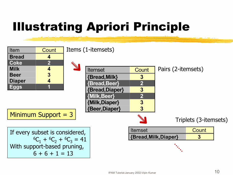
If every subset is considered, 6C1 + 6C2 + 6C3 = 41
With support-based pruning,6 + 6 + 1 = 13
IPAM Tutorial-January 2002-Vipin Kumar 11
Apriori Algorithm
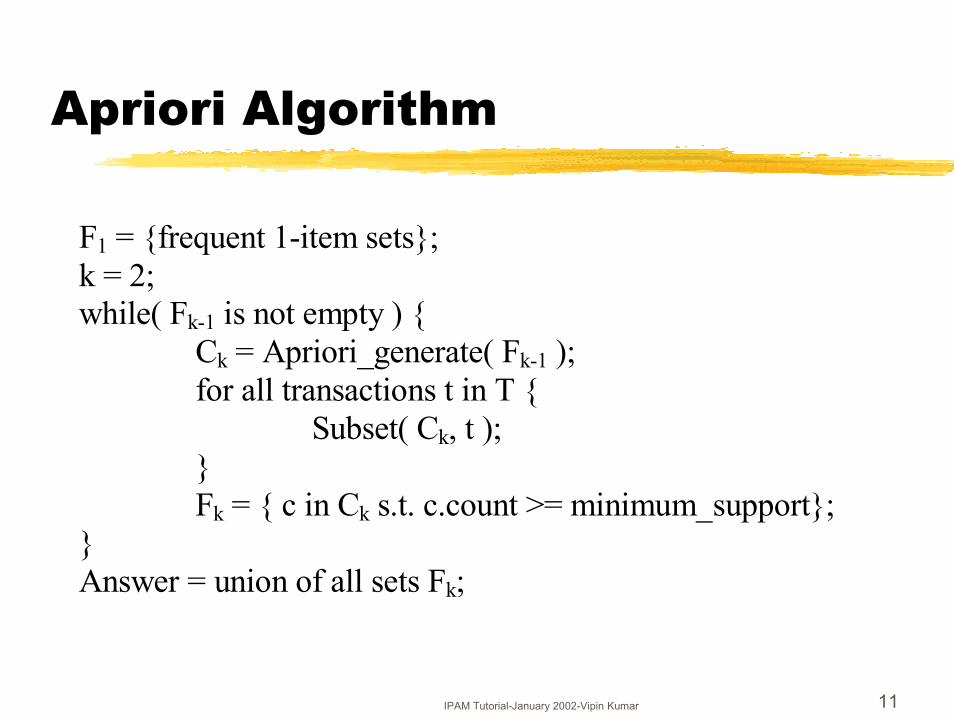
F1 = {frequent 1-item sets};k = 2;while( Fk-1 is not empty ) {
Ck = Apriori_generate( Fk-1 );for all transactions t in T {
Subset( Ck, t );}Fk = { c in Ck s.t. c.count >= minimum_support};
}Answer = union of all sets Fk;
IPAM Tutorial-January 2002-Vipin Kumar 12
Association Rule Discovery: Apriori_generate
Apriori_generate( F(k-1) ) {join Fk-1 with Fk-1 such that, c1 = (i1 , i2 , .. , ik-1) and c2 = (j1 , j2 , .. , jk-1) join together if ip = jp for 1 <= p <= k-1,and then new candidate, c, has a form c = (i1,i2,..,ik-1, jk-1).c is then added to a hash-tree structure.
}
IPAM Tutorial-January 2002-Vipin Kumar 13
Counting Candidates
�Frequent Itemsets are found by counting candidates.
�Simple way: �Search for each candidate in each transaction.
Expensive!!!
TransactionsCandidates
MN
IPAM Tutorial-January 2002-Vipin Kumar 14
Association Rule Discovery: Hash tree for fast access.
Candidate Hash TreeHash Function
1,4,7
2,5,8
3,6,9
1 5 9
1 4 5 1 3 63 4 5 3 6 7
3 6 83 5 63 5 76 8 9
2 3 45 6 7
1 2 44 5 7
1 2 54 5 8
IPAM Tutorial-January 2002-Vipin Kumar 15
Association Rule Discovery: Subset Operation
1,4,7
2,5,8
3,6,9
Hash Function1 2 3 5 6 transaction
1 5 9
1 4 5 1 3 63 4 5 3 6 7
3 6 83 5 63 5 76 8 9
2 3 45 6 7
1 2 44 5 7
1 2 54 5 8
1 + 2 3 5 6 3 5 62 +
5 63 +
IPAM Tutorial-January 2002-Vipin Kumar 16
Association Rule Discovery: Subset Operation (contd.)
1,4,7
2,5,8
3,6,9
Hash Function1 2 3 5 6 transaction
1 5 9
1 4 5 1 3 63 4 5 3 6 7
3 6 83 5 63 5 76 8 9
2 3 45 6 7
1 2 44 5 7
1 2 54 5 8
3 5 61 2 +
5 61 3 +
61 5 +
3 5 62 +
5 63 +
1 + 2 3 5 6
IPAM Tutorial-January 2002-Vipin Kumar 17
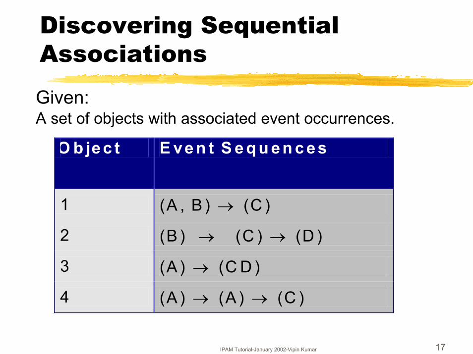
Discovering Sequential Associations
Given:A set of objects with associated event occurrences.
O b je c t E ve n t S e q u en c e s
1 (A , B ) � (C )
2 (B ) � (C ) � (D )
3 (A ) � (C D )
4 (A ) � (A ) � (C ) 10
IPAM Tutorial-January 2002-Vipin Kumar 18
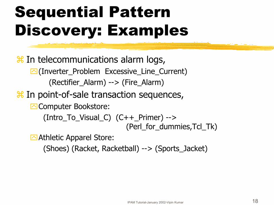
Sequential Pattern Discovery: Examples
� In telecommunications alarm logs,�(Inverter_Problem Excessive_Line_Current)
(Rectifier_Alarm) --> (Fire_Alarm)
� In point-of-sale transaction sequences,�Computer Bookstore:
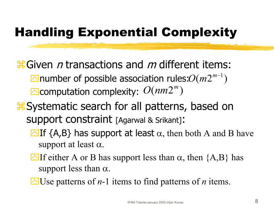
� Much higher computational complexity than association rule discovery.�O(mk 2k-1) number of possible sequential patterns having k
events, where m is the total number of possible events.
� Time constraints offer some pruning. Further use of support based pruning contains complexity.�A subsequence of a sequence occurs at least as many times as the
sequence.�A sequence has no more occurrences than any of its
subsequences.�Build sequences in increasing number of events. [GSP algorithm by
Agarwal & Srikant]
IPAM Tutorial-January 2002-Vipin Kumar 20
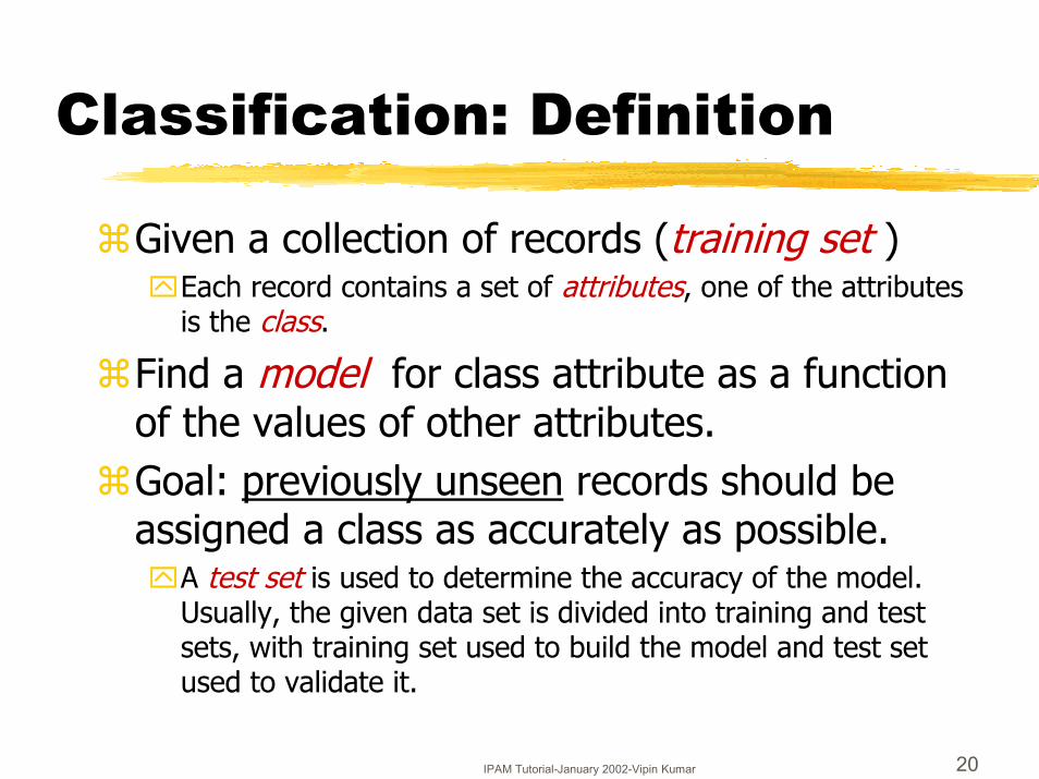
Classification: Definition
�Given a collection of records (training set )�Each record contains a set of attributes, one of the attributes
is the class.
�Find a model for class attribute as a function of the values of other attributes.
�Goal: previously unseen records should be assigned a class as accurately as possible.�A test set is used to determine the accuracy of the model.
Usually, the given data set is divided into training and test sets, with training set used to build the model and test set used to validate it.
IPAM Tutorial-January 2002-Vipin Kumar 21
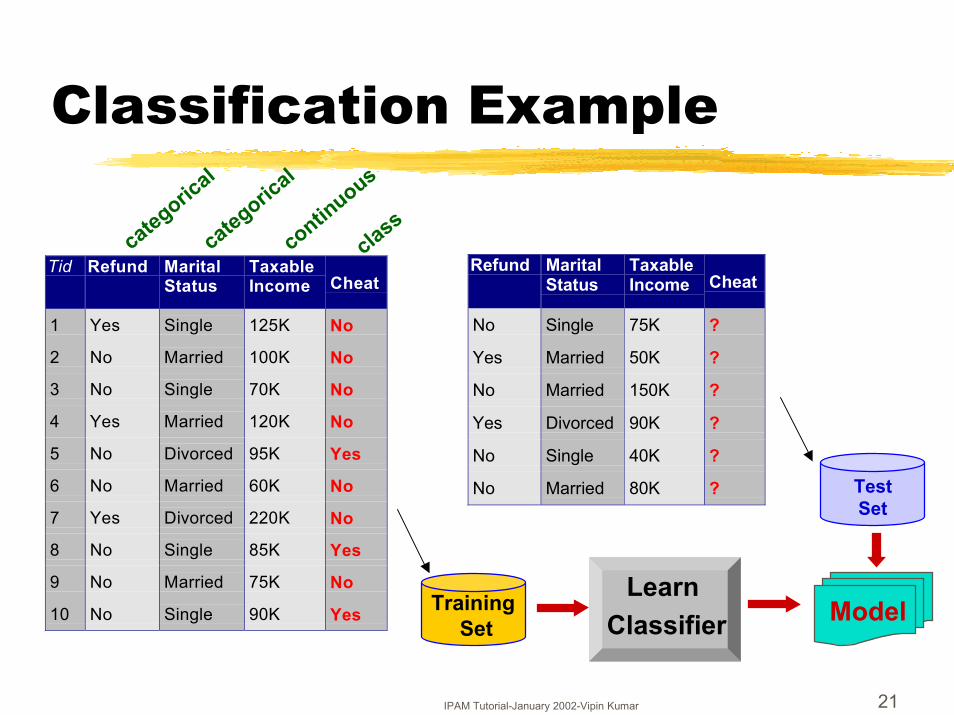
Classification Example
Tid Refund MaritalStatus
TaxableIncome Cheat
1 Yes Single 125K No
2 No Married 100K No
3 No Single 70K No
4 Yes Married 120K No
5 No Divorced 95K Yes
6 No Married 60K No
7 Yes Divorced 220K No
8 No Single 85K Yes
9 No Married 75K No
10 No Single 90K Yes10
Refund MaritalStatus
TaxableIncome Cheat
No Single 75K ?
Yes Married 50K ?
No Married 150K ?
Yes Divorced 90K ?
No Single 40K ?
No Married 80K ?10
TestSet
Training Set
ModelLearn
Classifier
categori
categori
continuo
classcal
cal us
IPAM Tutorial-January 2002-Vipin Kumar 22
Classifying Galaxies Courtsey: http://aps.umn.edu
Early
Intermediate
Late
Class: • Stages of Formation
Attributes:• Image features, • Characteristics of light
waves received, etc.
Data Size: • 72 million stars, 20 million galaxies• Object Catalog: 9 GB• Image Database: 150 GB
IPAM Tutorial-January 2002-Vipin Kumar 23
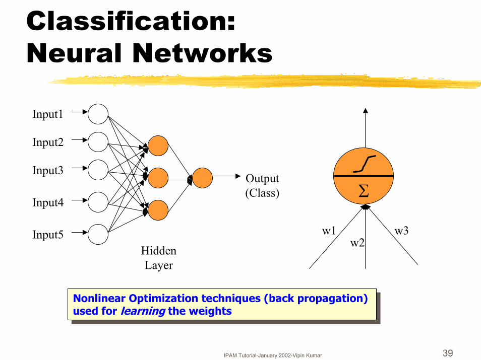
Classification Approaches
� Decision Tree based Methods� Rule-based Methods� Memory based reasoning� Neural Networks� Genetic Algorithms� Bayesian Networks� Support Vector Machines� Meta Algorithms
• Boosting• Bagging
IPAM Tutorial-January 2002-Vipin Kumar 24
Decision Tree Based Classification
�Decision tree models are better suited for data mining:�Inexpensive to construct�Easy to Interpret�Easy to integrate with database systems�Comparable or better accuracy in many applications
IPAM Tutorial-January 2002-Vipin Kumar 25
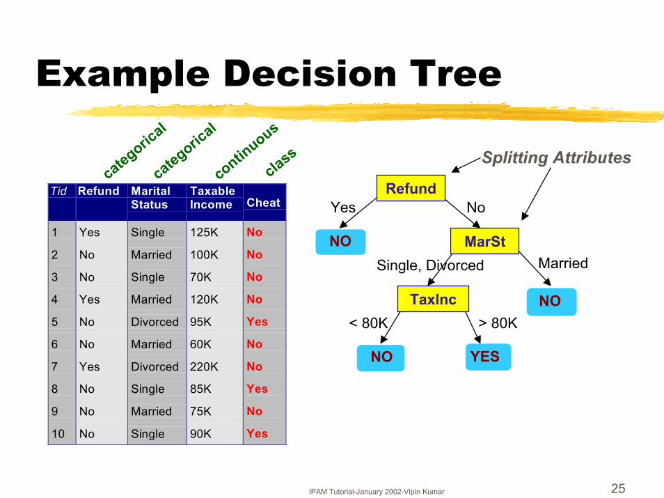
Example Decision Tree
Tid Refund MaritalStatus
TaxableIncome Cheat
1 Yes Single 125K No
2 No Married 100K No
3 No Single 70K No
4 Yes Married 120K No
5 No Divorced 95K Yes
6 No Married 60K No
7 Yes Divorced 220K No
8 No Single 85K Yes
9 No Married 75K No
10 No Single 90K Yes10
categori
categori
continuo
classcal
cal us
No
Splitting Attributes
YES
> 80K
NO
< 80K
MarriedNO
YesRefund
MarStSingle, Divorced
TaxInc NO
IPAM Tutorial-January 2002-Vipin Kumar 26
Decision Tree Algorithms
�Many Algorithms:�Hunt’s Algorithm (one of the earliest).�CART�ID3, C4.5�SLIQ,SPRINT
�General Structure:�Tree Induction�Tree Pruning
IPAM Tutorial-January 2002-Vipin Kumar 27
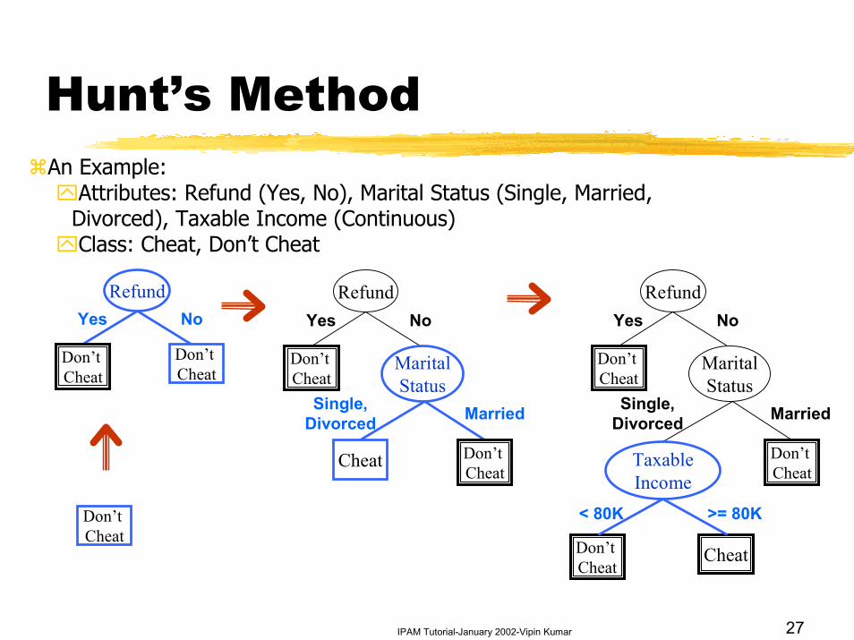
Hunt’s Method�An Example:
�Attributes: Refund (Yes, No), Marital Status (Single, Married, Divorced), Taxable Income (Continuous)
�Class: Cheat, Don’t Cheat
Refund
Don’t Cheat
Don’t Cheat
Yes NoRefund
Don’t Cheat
Yes No
MaritalStatus
Don’t Cheat
Cheat
Single,Divorced Married
Refund
Don’t Cheat
Yes No
MaritalStatus
Don’t Cheat
Cheat
Single,Divorced Married
TaxableIncome
Don’t Cheat
< 80K >= 80KDon’t Cheat
IPAM Tutorial-January 2002-Vipin Kumar 28
Tree Induction
�Greedy strategy.�Choose to split records based on an attribute
that optimizes the splitting criterion.
�Two phases at each node:�Split Determining Phase:
�How to Split a Given Attribute? �Which attribute to split on? Use Splitting Criterion.
�Splitting Phase: �Split the records into children.
IPAM Tutorial-January 2002-Vipin Kumar 29
Splitting Based on Categorical Attributes� Each partition has a subset of values signifying it.� Simple method: Use as many partitions as distinct
values.
� Complex method: Two partitions. Each partitioning divides values into two subsets. Need to find optimal partitioning.
CarTypeFamily
SportsLuxury
CarType{Sports,Luxury} {Family}
CarType{Family,Luxury} {Sports}OR
IPAM Tutorial-January 2002-Vipin Kumar 30
Splitting Based on Continuous Attributes
�Different ways of handling�Static: Apriori Discretization to form a categorical
attribute�may not be desirable in many situations
�Dynamic: Make decisions as algorithm proceeds�complex but more powerful and flexible in approximating
true dependency
IPAM Tutorial-January 2002-Vipin Kumar 31
Splitting Criterion: GINI
�Gini Index:
(NOTE: p( j | t) is the relative frequency of class j at node t).
�Measures impurity of a node. �Maximum (1 - 1/nc) when records are equally distributed
among all classes, implying least interesting information�Minimum (0.0) when all records belong to one class,
implying most interesting information
���
jtjptGINI 2)]|([1)(
C1 0C2 6
Gini=0.000
C1 1C2 5
Gini=0.278
C1 2C2 4
Gini=0.444
C1 3C2 3
Gini=0.500
IPAM Tutorial-January 2002-Vipin Kumar 32
Splitting Based on GINI
� Used in CART, SLIQ, SPRINT.� Splitting Criterion: Minimize Gini Index of the Split.� When a node p is split into k partitions (children), the
quality of split is computed as,
where, ni = number of records at child i,n = number of records at node p.
��
�
k
i
isplit iGINI
nnGINI
1)(
IPAM Tutorial-January 2002-Vipin Kumar 33
Binary Attributes: Computing GINI Index
�Splits into two partitions�Effect of Weighing partitions:
�Larger and Purer Partitions are sought for.
True?
Yes No
Node N1 Node N2
N1 N2C1 0 4C2 6 0Gini=0.000
N1 N2C1 3 4C2 3 0Gini=0.300
N1 N2C1 4 2C2 4 0Gini=0.400
N1 N2C1 6 2C2 2 0Gini=0.300
IPAM Tutorial-January 2002-Vipin Kumar 34
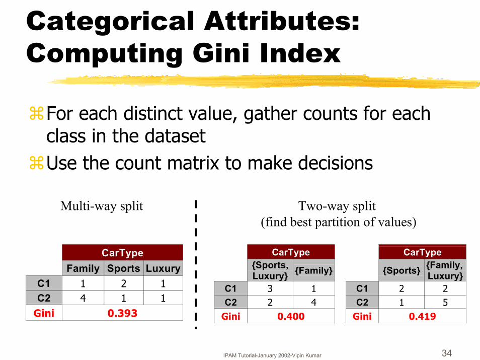
Categorical Attributes: Computing Gini Index
�For each distinct value, gather counts for each class in the dataset
�Use the count matrix to make decisions
CarType{Sports,Luxury} {Family}
C1 3 1C2 2 4
Gini 0.400
CarType
{Sports} {Family,Luxury}
C1 2 2C2 1 5
Gini 0.419
CarTypeFamily Sports Luxury
C1 1 2 1C2 4 1 1
Gini 0.393
Multi-way split Two-way split (find best partition of values)
IPAM Tutorial-January 2002-Vipin Kumar 35
Continuous Attributes: Computing Gini Index
� Use Binary Decisions based on one value� Several Choices for the splitting value
�Number of possible splitting values = Number of distinct values
� Each splitting value has a count matrix associated with it�Class counts in each of the partitions, A < v and A >= v
� Simple method to choose best v�For each v, scan the database to gather count matrix and
compute its Gini index�Computationally Inefficient! Repetition of work.
IPAM Tutorial-January 2002-Vipin Kumar 36
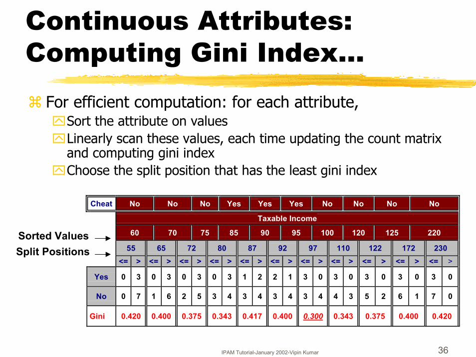
Continuous Attributes: Computing Gini Index...� For efficient computation: for each attribute,
�Sort the attribute on values�Linearly scan these values, each time updating the count matrix
and computing gini index�Choose the split position that has the least gini index
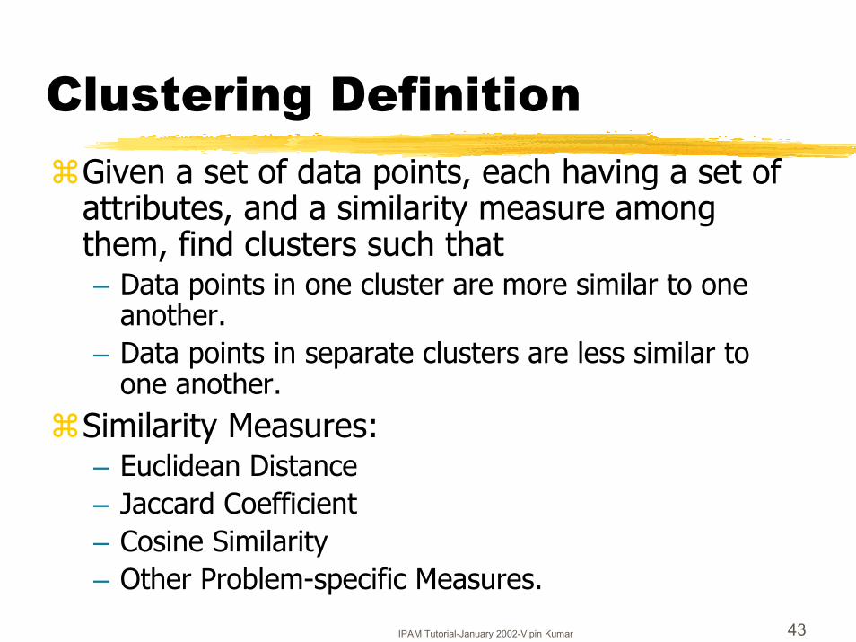
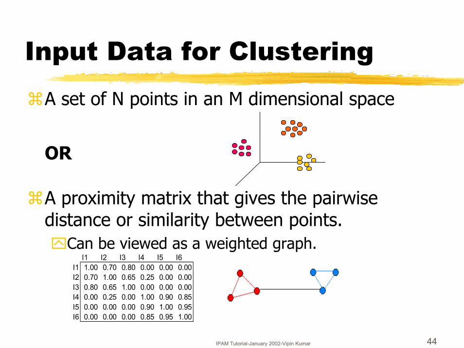
�Partitional Clustering ( K-means and K-medoid) finds a one-level partitioning of the data into K disjoint groups.
�Hierarchical Clustering finds a hierarchy of nested clusters (dendogram).�May proceed either
bottom-up (agglomerative) or top-down (divisive).
�Uses a proximity matrix.�Can be viewed as operating on a proximity graph.
IPAM Tutorial-January 2002-Vipin Kumar 46
K-means Clustering�Find a single partition of the data into K clusters
such that the within cluster error, e.g., , is minimized.
�Basic K-means Algorithm:1. Select K points as the initial centroids.2. Assign all points to the closest centroid.3. Recompute the centroids.4. Repeat steps 2 and 3 until the centroids don’t change.
�K-means is a gradient-descent algorithm that always converges - perhaps to a local minimum. (Clustering for Applications, Anderberg)
� �� �
�
K
1i Cx
2i
i
cx�
��
IPAM Tutorial-January 2002-Vipin Kumar 47
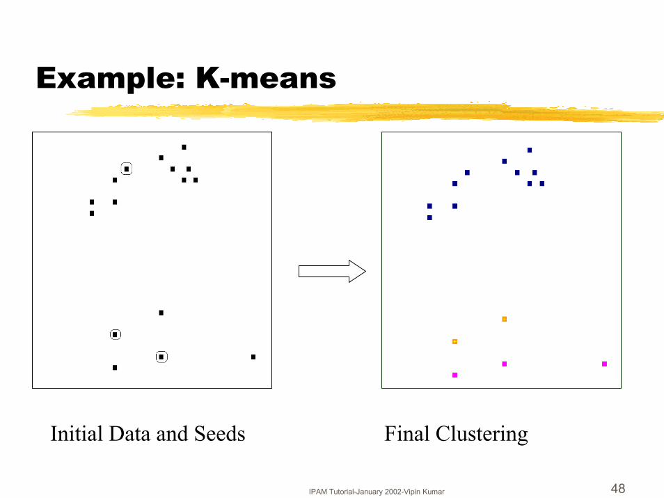
Example: Kmeans
Initial Data and Seeds Final Clustering
IPAM Tutorial-January 2002-Vipin Kumar 48
Example: K-means
Initial Data and Seeds Final Clustering
IPAM Tutorial-January 2002-Vipin Kumar 49
K-means: Initial Point Selection
�Bad set of initial points gives a poor solution.
�Random selection �Simple and efficient.�Initial points don’t cover clusters with high probability. �Many runs may be needed for optimal solution.
�Choose initial points from �Dense regions so that the points are “well-separated.”
�Many more variations on initial point selection.
IPAM Tutorial-January 2002-Vipin Kumar 50
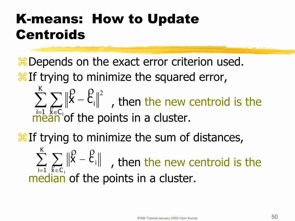
K-means: How to Update Centroids
�Depends on the exact error criterion used.�If trying to minimize the squared error,
, then the new centroid is themean of the points in a cluster.
�If trying to minimize the sum of distances,
, then the new centroid is the median of the points in a cluster.
��� �
�
K
1i Cxi
i
cx�
�� 2
� �� �
�
K
1i Cxi
i
cx�
��
IPAM Tutorial-January 2002-Vipin Kumar 51
K-means: Pre and Post Processing
�Outliers can dominate the clustering and, in some cases, are eliminated by preprocessing.
�Post-processing attempts to “fix-up” the clustering produced by the K-means algorithm.�Merge clusters that are “close” to each other.�Split “loose” clusters that contribute most to the error.�Permanently eliminate “small” clusters since they may represent
groups of outliers.
�Approaches are based on heuristics and require the user to choose parameter values.
IPAM Tutorial-January 2002-Vipin Kumar 52
K-means: Time and Space requirements
�O(MN) space since it uses just the vectors, not the proximity matrix.�M is the number of attributes.�N is the number of points.�Also keep track of which cluster each point belongs to
and the K cluster centers.
�Time for basic K-means is O(T*K*M*N),�T is the number of iterations. (T is often small, 5-10, and
can easily be bounded, as few changes occur after the first few iterations).
IPAM Tutorial-January 2002-Vipin Kumar 53
K-means: Determining the Number of Clusters
�Mostly heuristic and domain dependant approaches.
�Plot the error for 2, 3, … clusters and find the knee in the curve.
�Use domain specific knowledge and inspect the clusters for desired characteristics.
IPAM Tutorial-January 2002-Vipin Kumar 54
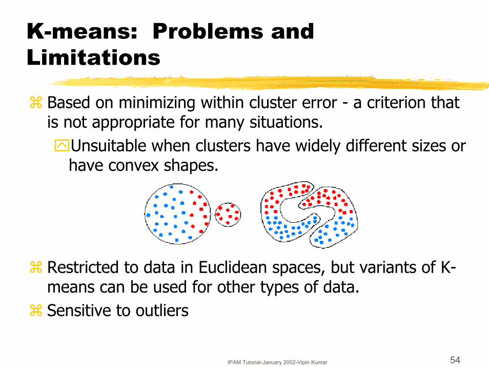
K-means: Problems and Limitations
� Based on minimizing within cluster error - a criterion that is not appropriate for many situations.�Unsuitable when clusters have widely different sizes or
have convex shapes.
� Restricted to data in Euclidean spaces, but variants of K-means can be used for other types of data.
� Sensitive to outliers
IPAM Tutorial-January 2002-Vipin Kumar 55
Hierarchical Clustering Algorithms
�Hierarchical Agglomerative Clustering1. Initially each item belongs to a single cluster.2. Combine the two most similar clusters.3. Repeat step 2 until there is only a single cluster.�Most popular approach.
�Hierarchical Divisive Clustering�Starting with a single cluster, divide clusters until
only single item clusters remain.�Less popular, but equivalent in functionality.
IPAM Tutorial-January 2002-Vipin Kumar 56
Cluster Similarity: MIN or Single Link �Similarity of two clusters is based on the two
most similar (closest) points in the different clusters.�Determined by one pair of points, i.e., by one link
in the proximity graph.
�Can handle non-elliptical shapes.�Sensitive to noise and outliers.
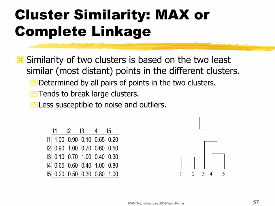
� Similarity of two clusters is based on the two least similar (most distant) points in the different clusters.�Determined by all pairs of points in the two clusters.�Tends to break large clusters.�Less susceptible to noise and outliers.
Cluster Similarity: Centroid Methods� Similarity of two clusters is based on the distance of
the centroids of the two clusters.
� Similar to K-means �Euclidean distance requirement�Problems with different sized clusters and convex shapes.
� Variations include “median” based methods.
IPAM Tutorial-January 2002-Vipin Kumar 60
Hierarchical Clustering: Time and Space requirements
�O(N2) space since it uses the proximity matrix. �N is the number of points.
�O(N3) time in many cases.�There are N steps and at each step the size, N2,
proximity matrix must be updated and searched.�By being careful, the complexity can be reduced to
O(N2 log(N) ) time for some approaches.
IPAM Tutorial-January 2002-Vipin Kumar 61
Hierarchical Clustering: Problems and Limitations
�Once a decision is made to combine two clusters, it cannot be undone.
�No objective function is directly minimized.�Different schemes have problems with one or
more of the following:�Sensitivity to noise and outliers. �Difficulty handling different sized clusters and convex
shapes.�Breaking large clusters.
IPAM Tutorial-January 2002-Vipin Kumar 62
Recent Approaches: CURE
� Uses a number of points to represent a cluster.� Representative points are found by selecting a constant
number of points from a cluster and then “shrinking” them toward the center of the cluster.
� Cluster similarity is the similarity of the closest pair of representative points from different clusters.
� Shrinking representative points toward the center helps avoid problems with noise and outliers.
� CURE is better able to handle clusters of arbitrary shapes and sizes.
(CURE, Guha, Rastogi, Shim)
IPAM Tutorial-January 2002-Vipin Kumar 63
Experimental ResultsCURE
(centroid) (single link)
Picture from CURE, Guha, Rastogi, Shim.
IPAM Tutorial-January 2002-Vipin Kumar 64
Limitations of Current Merging Schemes
�Existing merging schemes are static in nature.
IPAM Tutorial-January 2002-Vipin Kumar 65
Chameleon: Clustering Using Dynamic Modeling� Adapt to the characteristics of the data set to find the
natural clusters.� Use a dynamic model to measure the similarity between
clusters.�Main property is the relative closeness and relative inter-
connectivity of the cluster.�Two clusters are combined if the resulting cluster shares certain
properties with the constituent clusters.�The merging scheme preserves self-similarity.
� One of the areas of application is spatial data.
IPAM Tutorial-January 2002-Vipin Kumar 66
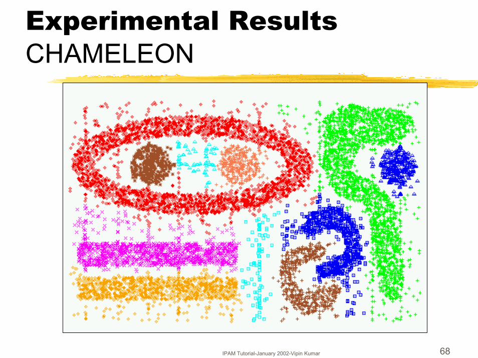
Experimental ResultsCHAMELEON
IPAM Tutorial-January 2002-Vipin Kumar 67
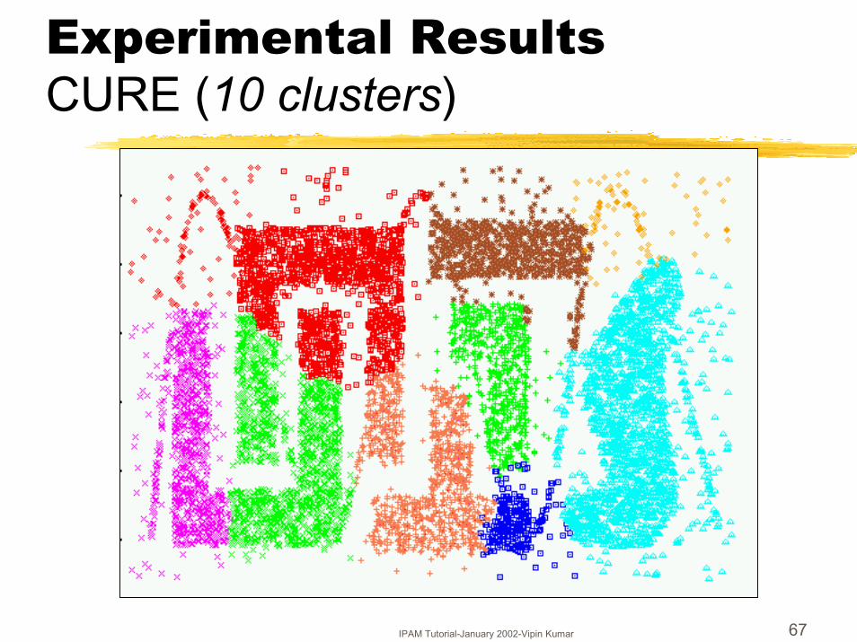
Experimental ResultsCURE (10 clusters)
IPAM Tutorial-January 2002-Vipin Kumar 68
Experimental ResultsCHAMELEON
IPAM Tutorial-January 2002-Vipin Kumar 69
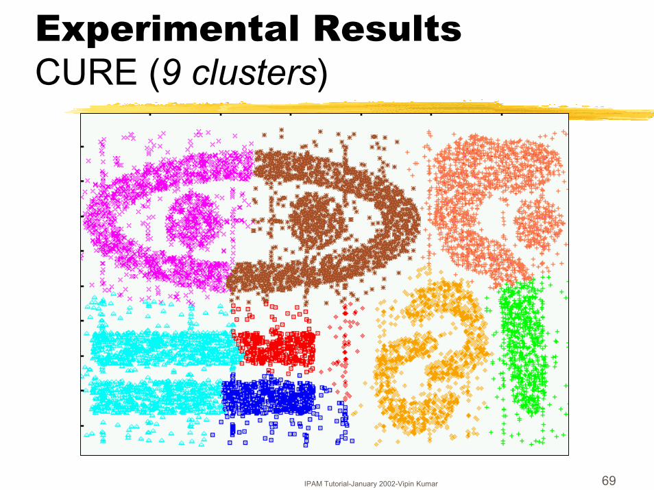
Experimental ResultsCURE (9 clusters)
IPAM Tutorial-January 2002-Vipin Kumar 70
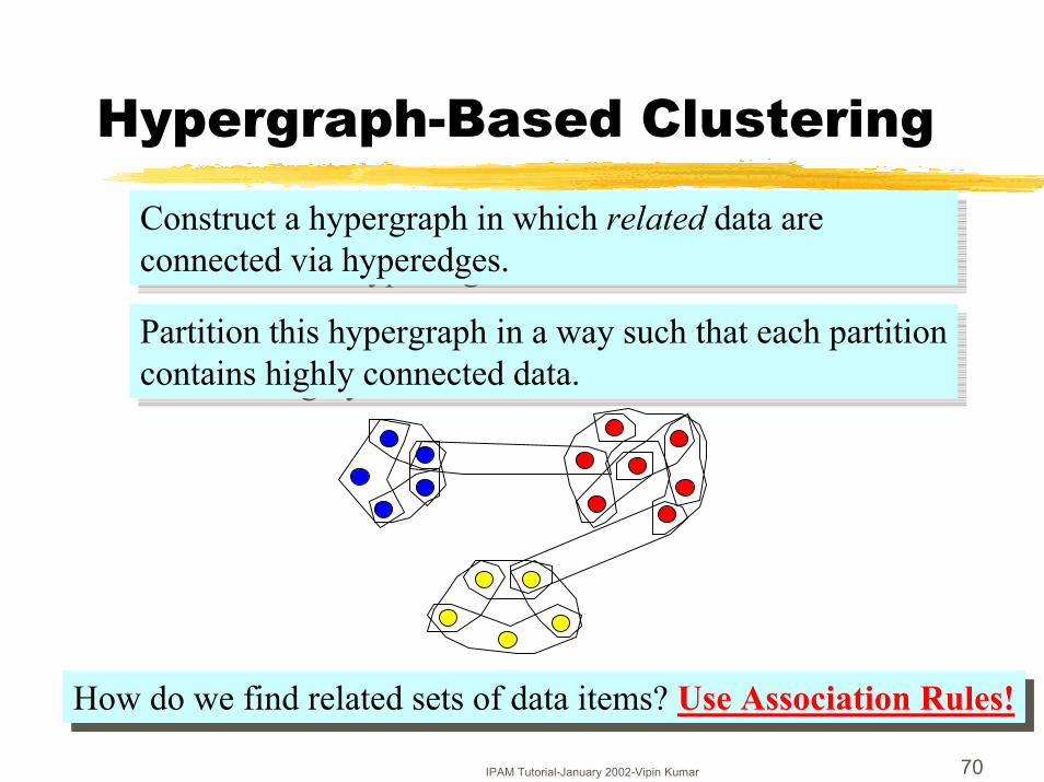
Hypergraph-Based Clustering
Construct a hypergraph in which related data are connected via hyperedges.Construct a hypergraph in which related data are connected via hyperedges.
Partition this hypergraph in a way such that each partition contains highly connected data.Partition this hypergraph in a way such that each partition contains highly connected data.
How do we find related sets of data items? Use Association Rules!How do we find related sets of data items? Use Association Rules!
IPAM Tutorial-January 2002-Vipin Kumar 71
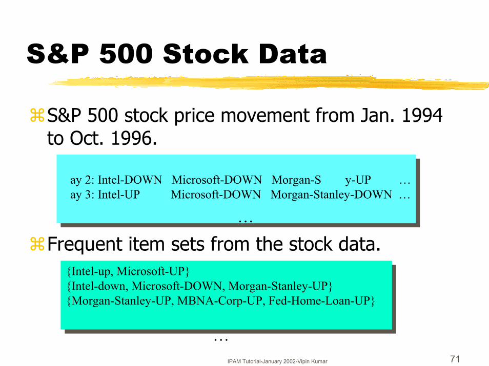
S&P 500 Stock Data
�S&P 500 stock price movement from Jan. 1994 to Oct. 1996.
�Frequent item sets from the stock data.
Day 1: Intel-UP Microsoft-UP Morgan-Stanley-DOWN …DD
�Feature transformation.�Normalizing features to the same scale by subtracting
the mean and dividing by the standard deviation.
�Feature Selection�As in classification, not all features are equally
important.
ReferencesBook References:[1] Hillol Kargupta and Philip Chan (Edotors), Advances in Distributed and Parallel Knowledge Discovery, AAAI Press, 2000.[2] Usama Fayyad, Gregory Piatetsky-Shapiro, Padhraic Smyth, and Ramasamy Uthurasamy (eds.), Advances in Knowledge Discovery and Data Mining, AAAI Press/ The MIT Press, 1996. [3] A. K. Jain and R. C. Dubes, Algorithms for Clustering Data, Prentice Hall, 1988.[4] Michael Anderberg, Clustering for Applications. Academic Press, 1973.[5] Jaiwei Han and Micheline Kamber, Data Mining: Concepts and Techniques, Morgan Kaufman, 2001.[6] Robert L. Grossman, Chandrika Kamath, Philip Kegelmeyer,Vipin Kumar, and Raju Namburu (Editors), Data Mining for Scientific and Engineering Applications,Kluwer Academic Publishers, 2001.[7] Michael Berry and Gordon Linoff, Data Mining Techniques (For Marketing, Sales, and Customer Support), John Wiley & Sons, 1997.[8] Kaufman and Rousseeuw, Finding Groups in Data: An Introduction to Cluster Analysis, Wiley, 1990.[9] Vipin Kumar, Ananth Grama, Anshul Gupta, and George Karypis, Introduction to Parallel Computing: Algorithm Design and Analysis, Benjamin Cummings/Addison Wesley, Redwood City, 1994.
ReferencesBook References:[10] Tom M. Mitchell, Machine Learning, WCB/McGraw-Hill, 1997.[8] Alex Freitasand Simon Lavington, Mining Very Large Databases with Parallel Processing,Kluwer Academic Publishers, 1998.[11] Sholom M. Weiss and Nitin Indurkhya, Predictive Data Mining (a practical guide), Morgan Kaufmann Publishers,1998.[12] David J. Hand, Heikki Mannila and Padhraic Smyth, Principles of Data Mining, The MIT Press, 2001.[13] J. Ross Quinlan, C4.5: Programs for Machine Learning, Morgan Kaufmann, 1993.[14] T. Kohonen, Self-Organizing Maps., Second Extended Edition, Springer Series in Information Sciences, Vol. 30, Springer, Berlin, Heidelberg, New York, 1997.
Research Paper References:[1] M. Mehta, R. Agarwal, and J. Rissanen, SLIQ: A Fast Scalable Classifier for Data Mining, Proc. Of the fifth Int. Conf. On Extending Database Technology (EDBT), Avignon, France, 1996.[2] J. Shafer, R. Agrawal, and M. Mehta, SPRINT: A Scalable Parallel Classifier for Data Mining, Proc. 22nd Int. Conf. On Very Large Databases, Mumbai, India, 1996.[3] A. Srivastava, E.H. Han, V. Kumar, and V.Singh, Parallel Formulations of Decision-Tree Classification Algorithms, Proc. 12th International Parallel Processing Symposium (IPPS), Orlando, 1998.[4] M.Joshi, G.Karypis, and V. Kumar, ScalParC: A New Scalable and Efficient Parallel Classification Algorithms for Mining Large Datasets, Proc. 12th International Parallel Processing Symposium (IPPS), Orlando, 1998.[5] N. Friedman, D. Geiger, and M. Goldszmidt, Bayesian Network Classifiers,Machine Learning 29:131--163, 1997.[6] R. Agrawal, T.Imielinski, and A.Swami, Mining Association Rules Between Sets of Items in Large Databases, Proc. 1993 ACM-SIGMOD Int.Conf. On Management of Data, Washington, D.C., 1993.[7] R. Agrawal and R. Srikant, Fast Algorithms for Mining Association Rules, Proc. Of 20th VLDB Conference, 1994.
References...
References...[8] R. Agrawal and J.C. Shafer, Parallel Mining of Association Rules, IEEE Trans. On Knowledge and Data Eng., 8(6):962-969, December 1996.[9] E.H.Han, G.Karypis, and V.Kumar, Scalable Parallel Data Mining for Association Rules, Proc. 1997 ACM-SIGMOD Int. Conf. On Management of Data, Tucson, Arizona, 1997.[10] R. Srikant and R. Agrawal, Mining Sequential Patterns: Generalizations and Performance Improvements, Proc. Of 5th Int. Conf. On Extending Database Technology (EDBT), Avignon, France, 1996.[11] M. Joshi, G. Karypis, and V. Kumar, Parallel Algorithms for Sequential Associations: Issues and Challenges, Mini-symposium Talk at Ninth SIAM International Conference on Parallel Processing (PP’99), San Antonio, 1999.[12] George Karypis, Eui-Hong (Sam) Han, and Vipin Kumar, CHAMELEON: A Hierarchical Clustering Algorithm Using Dynamic Modeling (1999), IEEE Computer, Vol. 32, No. 8, August, 1999. pp. 68-75.[13] George Karypis, Eui-Hong (Sam) Han, and Vipin Kumar, Multilevel Refinement for Hierarchical Clustering (1999)., Technical Report # 99-020. [14] Daniel Boley, Maria Gini, Robert Gross, Eui-Hong (Sam) Han, Kyle Hastings, George Karypis, Vipin Kumar, Bamshad Mobasher, and Jerome Moore,Partitioning-Based Clustering for Web Document Categorization (1999). To appear in Decision Support Systems Journal.
[15] Eui-Hong (Sam) Han, George Karypis, Vipin Kumar and B. Mobasher,Hypergraph Based Clustering in High-Dimensional Data Sets: A Summary of Results (1998). Bulletin of the Technical Committee on Data Engineering, Vol. 21, No. 1, 1998.[16] K. C. Gowda and G. Krishna, Agglomerative Clustering Using the Concept of Mutual Nearest Neighborhood, Pattern Recognition, Vol. 10, pp. 105-112, 1978.[17] Rakesh Agrawal, Johannes Gehrke, Dimitrios Gunopulos, PrabhakarRaghavan, Automatic Subspace Clustering of High Dimensional Data for DataMining Applications, Proc. of the ACM SIGMOD Int'l Conference on Management of Data, Seattle, Washington, June 1998.[18] Peter Cheeseman and John Stutz, "Bayesian Classification (AutoClass): Theory and Results”, in U. M. Fayyad, G. Piatetsky-Shapiro, P. Smith, and R. Uthurusamy (eds.), "Advances in Knowledge Discovery and Data Mining", pp. 153-180, AAAI/MIT Press, 1996. [19] Tian Zhang, Raghu Ramakrishnan, Miron Livny, "BIRCH: An Efficient Data Clustering Method for Very Large Databases”, Proc. of ACM SIGMOD Int'l Conf. on Data Management, Canada, June 1996.
References...
[20] Venkatesh Ganti, Raghu Ramakrishnan, and Johannes Gehrke, "Clustering Large Datasets in Arbitrary Metric Spaces”, Proceedings of IEEE Conference on Data Engineering, Australia, 1999.[21] Jarvis and E. A. Patrick, Clustering Using a Similarity Measure Based on Shared Nearest Neighbors, IEEE Transactions on Computers, Vol. C-22, No. 11, November, 1973.[22] Sudipto Guha, Rajeev Rastogi, Kyuseok Shim, "CURE: An Efficient Clustering Algorithm for Large Databases”, ACM SIGMOD Conference, 1998, pp. 73-84.[23] Sander J., Ester M., Kriegel H.-P., Xu X., Density-Based Clustering in Spatial Databases: The Algorithm GDBSCAN and its Applications, Data Mining and Knowledge Discovery, An International Journal, Kluwer Academic Publishers, Vol. 2, No. 2, 1998, pp. 169-194.[24] R. Ng and J. Han., Efficient and effective clustering method for spatial data mining, In Proc. 1994 Int. Conf. Very Large Data Bases, pp. 144--155, Santiago, Chile, September, 1994.[25] Chris Fraley and Adrian E. Raftery, How many clusters? Which clustering method? - Answers via Model-Based Cluster Analysis, Computer Journal, 41(1998):578-588.
References...
[26] Sudipto Guha, Rajeev Rastogi, Kyuseok Shim, "ROCK: A Robust Clustering Algorithm for Categorical Attributes”, Proceedings of IEEE Conference on Data Engineering, Australia, 1999.[27] Paul S. Bradley, Usama M. Fayyad and Cory A. Reina, Scaling Clustering Algorithms to Large Databases, Proceedings of the 4th International Conference on Knowledge Discovery & Data Mining (KDD98).
Over 100 More Data Mining References are available at http://www.cs.umn.edu/~mjoshi/dmrefs.html
Our group’s papers are available via http://www.cs.umn.edu/~kumar


![Improving Association Rule based Data Mining Algorithms ... · The existing data mining algorithms for distributed data are of communication intensive [2]. Many algorithms for data](https://static.documents.pub/doc/80x56/6053a87355c223237f6c0867/improving-association-rule-based-data-mining-algorithms-the-existing-data-mining.jpg)


