Page 1
Data Mining Association Analysis: Basic Concepts
and Algorithms
Lecture Notes for Chapter 6
Introduction to Data Miningby
Tan, Steinbach, Kumar
© Tan,Steinbach, Kumar Introduction to Data Mining 4/18/2004 1
© Tan,Steinbach, Kumar Introduction to Data Mining 4/18/2004 2
Association Rule Mining
Given a set of transactions, find rules that will predict the occurrence of an item based on the occurrences of other items in the transaction
Market-Basket transactions
TID Items
1 Bread, Milk
2 Bread, Diaper, Beer, Eggs
3 Milk, Diaper, Beer, Coke 4 Bread, Milk, Diaper, Beer
5 Bread, Milk, Diaper, Coke
Example of Association Rules
{Diaper} → {Beer},{Milk, Bread} → {Eggs,Coke},{Beer, Bread} → {Milk},
Implication means co-occurrence, not causality!
Page 2
© Tan,Steinbach, Kumar Introduction to Data Mining 4/18/2004 3
Definition: Frequent Itemset
Itemset– A collection of one or more items
Example: {Milk, Bread, Diaper}
– k-itemsetAn itemset that contains k items
Support count (σ)– Frequency of occurrence of an itemset– E.g. σ({Milk, Bread,Diaper}) = 2
Support– Fraction of transactions that contain an
itemset– E.g. s({Milk, Bread, Diaper}) = 2/5
Frequent Itemset– An itemset whose support is greater
than or equal to a minsup threshold
TID Items
1 Bread, Milk
2 Bread, Diaper, Beer, Eggs
3 Milk, Diaper, Beer, Coke 4 Bread, Milk, Diaper, Beer
5 Bread, Milk, Diaper, Coke
© Tan,Steinbach, Kumar Introduction to Data Mining 4/18/2004 4
Definition: Association Rule
Example:Beer}Diaper,Milk{ ⇒
4.052
|T|)BeerDiaper,,Milk( === σs
67.032
)Diaper,Milk()BeerDiaper,Milk,(
===σ
σc
Association Rule– An implication expression of the form
X → Y, where X and Y are itemsets– Example:
{Milk, Diaper} → {Beer}
Rule Evaluation Metrics– Support (s)
Fraction of transactions that contain both X and Y
– Confidence (c)Measures how often items in Y appear in transactions thatcontain X
TID Items
1 Bread, Milk
2 Bread, Diaper, Beer, Eggs
3 Milk, Diaper, Beer, Coke 4 Bread, Milk, Diaper, Beer
5 Bread, Milk, Diaper, Coke
Page 3
© Tan,Steinbach, Kumar Introduction to Data Mining 4/18/2004 5
Association Rule Mining Task
Given a set of transactions T, the goal of association rule mining is to find all rules having – support ≥ minsup threshold– confidence ≥ minconf threshold
Brute-force approach:– List all possible association rules– Compute the support and confidence for each rule– Prune rules that fail the minsup and minconf
thresholds⇒ Computationally prohibitive!
© Tan,Steinbach, Kumar Introduction to Data Mining 4/18/2004 6
Mining Association Rules
Example of Rules:{Milk,Diaper} → {Beer} (s=0.4, c=0.67){Milk,Beer} → {Diaper} (s=0.4, c=1.0){Diaper,Beer} → {Milk} (s=0.4, c=0.67){Beer} → {Milk,Diaper} (s=0.4, c=0.67) {Diaper} → {Milk,Beer} (s=0.4, c=0.5) {Milk} → {Diaper,Beer} (s=0.4, c=0.5)
TID Items
1 Bread, Milk
2 Bread, Diaper, Beer, Eggs
3 Milk, Diaper, Beer, Coke 4 Bread, Milk, Diaper, Beer
5 Bread, Milk, Diaper, Coke
Observations:• All the above rules are binary partitions of the same itemset:
{Milk, Diaper, Beer}
• Rules originating from the same itemset have identical support butcan have different confidence
• Thus, we may decouple the support and confidence requirements
Page 4
© Tan,Steinbach, Kumar Introduction to Data Mining 4/18/2004 7
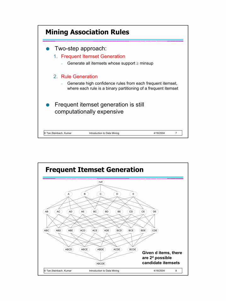
Mining Association Rules
Two-step approach: 1. Frequent Itemset Generation
– Generate all itemsets whose support ≥ minsup
2. Rule Generation– Generate high confidence rules from each frequent itemset,
where each rule is a binary partitioning of a frequent itemset
Frequent itemset generation is still computationally expensive
© Tan,Steinbach, Kumar Introduction to Data Mining 4/18/2004 8
Frequent Itemset Generation
null
AB AC AD AE BC BD BE CD CE DE
A B C D E
ABC ABD ABE ACD ACE ADE BCD BCE BDE CDE
ABCD ABCE ABDE ACDE BCDE
ABCDE
Given d items, there are 2d possible candidate itemsets
Page 5
© Tan,Steinbach, Kumar Introduction to Data Mining 4/18/2004 9
Frequent Itemset Generation
Brute-force approach: – Each itemset in the lattice is a candidate frequent itemset– Count the support of each candidate by scanning the
database
– Match each transaction against every candidate– Complexity ~ O(NMw) => Expensive since M = 2d !!!
TID Items 1 Bread, Milk 2 Bread, Diaper, Beer, Eggs 3 Milk, Diaper, Beer, Coke 4 Bread, Milk, Diaper, Beer 5 Bread, Milk, Diaper, Coke
N
Transactions List ofCandidates
M
w
© Tan,Steinbach, Kumar Introduction to Data Mining 4/18/2004 10
Computational Complexity
Given d unique items:– Total number of itemsets = 2d
– Total number of possible association rules:
123 1
1
1 1
+−=
−×
=
+
−
=
−
=∑ ∑
dd
d
k
kd
j jkd
kd
R
If d=6, R = 602 rules
Page 6
© Tan,Steinbach, Kumar Introduction to Data Mining 4/18/2004 11
Frequent Itemset Generation Strategies
Reduce the number of candidates (M)– Complete search: M=2d
– Use pruning techniques to reduce M
Reduce the number of transactions (N)– Reduce size of N as the size of itemset increases– Used by DHP and vertical-based mining algorithms
Reduce the number of comparisons (NM)– Use efficient data structures to store the candidates or
transactions– No need to match every candidate against every
transaction
© Tan,Steinbach, Kumar Introduction to Data Mining 4/18/2004 12
Reducing Number of Candidates
Apriori principle:– If an itemset is frequent, then all of its subsets must also
be frequent
Apriori principle holds due to the following property of the support measure:
– Support of an itemset never exceeds the support of its subsets
– This is known as the anti-monotone property of support
)()()(:, YsXsYXYX ≥⇒⊆∀
Page 7
© Tan,Steinbach, Kumar Introduction to Data Mining 4/18/2004 13
Found to be Infrequent
null
AB AC AD AE BC BD BE CD CE DE
A B C D E
ABC ABD ABE ACD ACE ADE BCD BCE BDE CDE
ABCD ABCE ABDE ACDE BCDE
ABCDE
Illustrating Apriori Principle
null
AB AC AD AE BC BD BE CD CE DE
A B C D E
ABC ABD ABE ACD ACE ADE BCD BCE BDE CDE
ABCD ABCE ABDE ACDE BCDE
ABCDEPruned supersets
© Tan,Steinbach, Kumar Introduction to Data Mining 4/18/2004 14
Illustrating Apriori Principle
Item CountBread 4Coke 2Milk 4Beer 3Diaper 4Eggs 1
Itemset Count{Bread,Milk} 3{Bread,Beer} 2{Bread,Diaper} 3{Milk,Beer} 2{Milk,Diaper} 3{Beer,Diaper} 3
I te m s e t C o u n t {B re a d ,M ilk ,D ia p e r} 3
Items (1-itemsets)
Pairs (2-itemsets)
(No need to generatecandidates involving Cokeor Eggs)
Triplets (3-itemsets)Minimum Support = 3
If every subset is considered, 6C1 + 6C2 + 6C3 = 41
With support-based pruning,6 + 6 + 1 = 13
Page 8
© Tan,Steinbach, Kumar Introduction to Data Mining 4/18/2004 15
Apriori Algorithm
Method:
– Let k=1– Generate frequent itemsets of length 1– Repeat until no new frequent itemsets are identified
Generate length (k+1) candidate itemsets from length k frequent itemsetsPrune candidate itemsets containing subsets of length k that are infrequent Count the support of each candidate by scanning the DBEliminate candidates that are infrequent, leaving only those that are frequent
© Tan,Steinbach, Kumar Introduction to Data Mining 4/18/2004 16
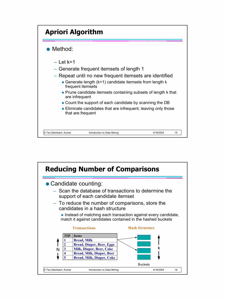
Reducing Number of Comparisons
Candidate counting:– Scan the database of transactions to determine the
support of each candidate itemset– To reduce the number of comparisons, store the
candidates in a hash structureInstead of matching each transaction against every candidate,
match it against candidates contained in the hashed buckets
TID Items 1 Bread, Milk 2 Bread, Diaper, Beer, Eggs 3 Milk, Diaper, Beer, Coke 4 Bread, Milk, Diaper, Beer 5 Bread, Milk, Diaper, Coke
N
Transactions Hash Structure
k
Buckets
Page 9
© Tan,Steinbach, Kumar Introduction to Data Mining 4/18/2004 17
Generate Hash Tree
2 3 45 6 7
1 4 5 1 3 6
1 2 44 5 7 1 2 5
4 5 81 5 9
3 4 5 3 5 63 5 76 8 9
3 6 73 6 8
1,4,72,5,8
3,6,9Hash function
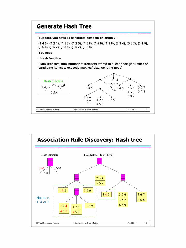
Suppose you have 15 candidate itemsets of length 3:
{1 4 5}, {1 2 4}, {4 5 7}, {1 2 5}, {4 5 8}, {1 5 9}, {1 3 6}, {2 3 4}, {5 6 7}, {3 4 5}, {3 5 6}, {3 5 7}, {6 8 9}, {3 6 7}, {3 6 8}
You need:
• Hash function
• Max leaf size: max number of itemsets stored in a leaf node (if number of candidate itemsets exceeds max leaf size, split the node)
© Tan,Steinbach, Kumar Introduction to Data Mining 4/18/2004 18
Association Rule Discovery: Hash tree
1 5 9
1 4 5 1 3 63 4 5 3 6 7
3 6 83 5 63 5 76 8 9
2 3 45 6 7
1 2 44 5 7
1 2 54 5 8
1,4,7
2,5,8
3,6,9
Hash Function Candidate Hash Tree
Hash on 1, 4 or 7
Page 10
© Tan,Steinbach, Kumar Introduction to Data Mining 4/18/2004 19
Association Rule Discovery: Hash tree
1 5 9
1 4 5 1 3 63 4 5 3 6 7
3 6 83 5 63 5 76 8 9
2 3 45 6 7
1 2 44 5 7
1 2 54 5 8
1,4,7
2,5,8
3,6,9
Hash Function Candidate Hash Tree
Hash on 2, 5 or 8
© Tan,Steinbach, Kumar Introduction to Data Mining 4/18/2004 20
Association Rule Discovery: Hash tree
1 5 9
1 4 5 1 3 63 4 5 3 6 7
3 6 83 5 63 5 76 8 9
2 3 45 6 7
1 2 44 5 7
1 2 54 5 8
1,4,7
2,5,8
3,6,9
Hash Function Candidate Hash Tree
Hash on 3, 6 or 9
Page 11
© Tan,Steinbach, Kumar Introduction to Data Mining 4/18/2004 21
Subset Operation
1 2 3 5 6
Transaction, t
2 3 5 61 3 5 62
5 61 33 5 61 2 61 5 5 62 3 62 5
5 63
1 2 31 2 51 2 6
1 3 51 3 6 1 5 6 2 3 5
2 3 6 2 5 6 3 5 6
Subsets of 3 items
Level 1
Level 2
Level 3
63 5
Given a transaction t, what are the possible subsets of size 3?
© Tan,Steinbach, Kumar Introduction to Data Mining 4/18/2004 22
Subset Operation Using Hash Tree
1 5 9
1 4 5 1 3 63 4 5 3 6 7
3 6 83 5 63 5 76 8 9
2 3 45 6 7
1 2 44 5 7
1 2 54 5 8
1 2 3 5 6
1 + 2 3 5 6 3 5 62 +
5 63 +
1,4,7
2,5,8
3,6,9
Hash Functiontransaction
Page 12
© Tan,Steinbach, Kumar Introduction to Data Mining 4/18/2004 23
Subset Operation Using Hash Tree
1 5 9
1 4 5 1 3 63 4 5 3 6 7
3 6 83 5 63 5 76 8 9
2 3 45 6 7
1 2 44 5 7
1 2 54 5 8
1,4,7
2,5,8
3,6,9
Hash Function1 2 3 5 6
3 5 61 2 +
5 61 3 +
61 5 +
3 5 62 +
5 63 +
1 + 2 3 5 6
transaction
© Tan,Steinbach, Kumar Introduction to Data Mining 4/18/2004 24
Subset Operation Using Hash Tree
1 5 9
1 4 5 1 3 63 4 5 3 6 7
3 6 83 5 63 5 76 8 9
2 3 45 6 7
1 2 44 5 7
1 2 54 5 8
1,4,7
2,5,8
3,6,9
Hash Function1 2 3 5 6
3 5 61 2 +
5 61 3 +
61 5 +
3 5 62 +
5 63 +
1 + 2 3 5 6
transaction
Match transaction against 11 out of 15 candidates
Page 13
© Tan,Steinbach, Kumar Introduction to Data Mining 4/18/2004 25
Factors Affecting Complexity
Choice of minimum support threshold– lowering support threshold results in more frequent itemsets– this may increase number of candidates and max length of
frequent itemsetsDimensionality (number of items) of the data set
– more space is needed to store support count of each item– if number of frequent items also increases, both computation and
I/O costs may also increaseSize of database
– since Apriori makes multiple passes, run time of algorithm may increase with number of transactions
Average transaction width– transaction width increases with denser data sets– This may increase max length of frequent itemsets and traversals
of hash tree (number of subsets in a transaction increases with its width)
© Tan,Steinbach, Kumar Introduction to Data Mining 4/18/2004 26
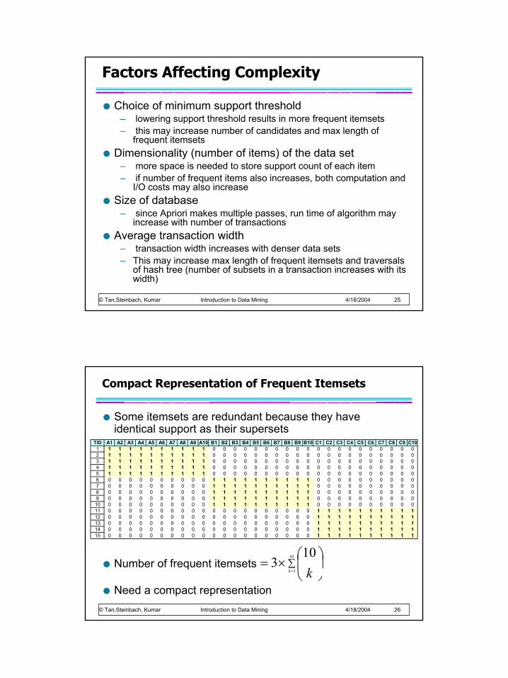
Compact Representation of Frequent Itemsets
Some itemsets are redundant because they have identical support as their supersets
Number of frequent itemsets
Need a compact representation
TID A1 A2 A3 A4 A5 A6 A7 A8 A9 A10 B1 B2 B3 B4 B5 B6 B7 B8 B9 B10 C1 C2 C3 C4 C5 C6 C7 C8 C9 C101 1 1 1 1 1 1 1 1 1 1 0 0 0 0 0 0 0 0 0 0 0 0 0 0 0 0 0 0 0 02 1 1 1 1 1 1 1 1 1 1 0 0 0 0 0 0 0 0 0 0 0 0 0 0 0 0 0 0 0 03 1 1 1 1 1 1 1 1 1 1 0 0 0 0 0 0 0 0 0 0 0 0 0 0 0 0 0 0 0 04 1 1 1 1 1 1 1 1 1 1 0 0 0 0 0 0 0 0 0 0 0 0 0 0 0 0 0 0 0 05 1 1 1 1 1 1 1 1 1 1 0 0 0 0 0 0 0 0 0 0 0 0 0 0 0 0 0 0 0 06 0 0 0 0 0 0 0 0 0 0 1 1 1 1 1 1 1 1 1 1 0 0 0 0 0 0 0 0 0 07 0 0 0 0 0 0 0 0 0 0 1 1 1 1 1 1 1 1 1 1 0 0 0 0 0 0 0 0 0 08 0 0 0 0 0 0 0 0 0 0 1 1 1 1 1 1 1 1 1 1 0 0 0 0 0 0 0 0 0 09 0 0 0 0 0 0 0 0 0 0 1 1 1 1 1 1 1 1 1 1 0 0 0 0 0 0 0 0 0 010 0 0 0 0 0 0 0 0 0 0 1 1 1 1 1 1 1 1 1 1 0 0 0 0 0 0 0 0 0 011 0 0 0 0 0 0 0 0 0 0 0 0 0 0 0 0 0 0 0 0 1 1 1 1 1 1 1 1 1 112 0 0 0 0 0 0 0 0 0 0 0 0 0 0 0 0 0 0 0 0 1 1 1 1 1 1 1 1 1 113 0 0 0 0 0 0 0 0 0 0 0 0 0 0 0 0 0 0 0 0 1 1 1 1 1 1 1 1 1 114 0 0 0 0 0 0 0 0 0 0 0 0 0 0 0 0 0 0 0 0 1 1 1 1 1 1 1 1 1 115 0 0 0 0 0 0 0 0 0 0 0 0 0 0 0 0 0 0 0 0 1 1 1 1 1 1 1 1 1 1
∑=
×=
10
1
103
k k
Page 14
© Tan,Steinbach, Kumar Introduction to Data Mining 4/18/2004 27
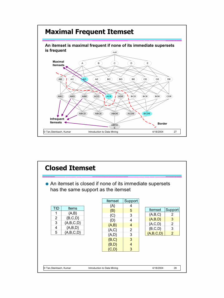
Maximal Frequent Itemset
null
AB AC AD AE BC BD BE CD CE DE
A B C D E
ABC ABD ABE ACD ACE ADE BCD BCE BDE CDE
ABCD ABCE ABDE ACDE BCDE
ABCDE
BorderInfrequent Itemsets
Maximal Itemsets
An itemset is maximal frequent if none of its immediate supersets is frequent
© Tan,Steinbach, Kumar Introduction to Data Mining 4/18/2004 28
Closed Itemset
An itemset is closed if none of its immediate supersets has the same support as the itemset
TID Items1 {A,B}2 {B,C,D}3 {A,B,C,D}4 {A,B,D}5 {A,B,C,D}
Itemset Support{A} 4{B} 5{C} 3{D} 4
{A,B} 4{A,C} 2{A,D} 3{B,C} 3{B,D} 4{C,D} 3
Itemset Support{A,B,C} 2{A,B,D} 3{A,C,D} 2{B,C,D} 3
{A,B,C,D} 2
Page 15
© Tan,Steinbach, Kumar Introduction to Data Mining 4/18/2004 29
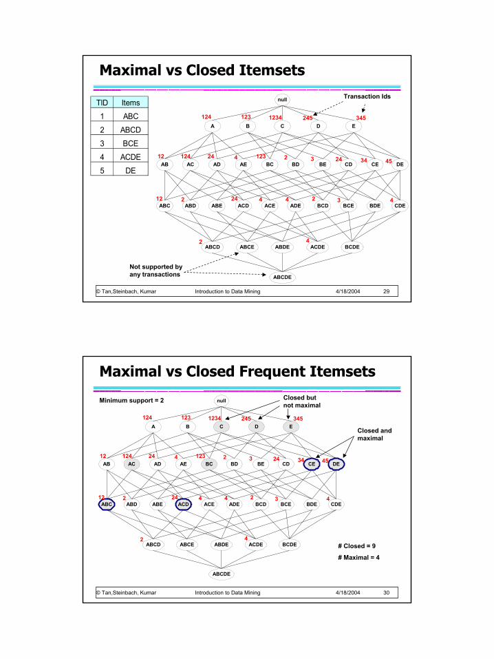
Maximal vs Closed Itemsets
TID Items
1 ABC
2 ABCD
3 BCE
4 ACDE
5 DE
null
AB AC AD AE BC BD BE CD CE DE
A B C D E
ABC ABD ABE ACD ACE ADE BCD BCE BDE CDE
ABCD ABCE ABDE ACDE BCDE
ABCDE
124 123 1234 245 345
12 124 24 4 123 2 3 24 34 45
12 2 24 4 4 2 3 4
2 4
Transaction Ids
Not supported by any transactions
© Tan,Steinbach, Kumar Introduction to Data Mining 4/18/2004 30
Maximal vs Closed Frequent Itemsets
null
AB AC AD AE BC BD BE CD CE DE
A B C D E
ABC ABD ABE ACD ACE ADE BCD BCE BDE CDE
ABCD ABCE ABDE ACDE BCDE
ABCDE
124 123 1234 245 345
12 124 24 4 123 2 3 24 34 45
12 2 24 4 4 2 3 4
2 4
Minimum support = 2
# Closed = 9
# Maximal = 4
Closed and maximal
Closed but not maximal
Page 16
© Tan,Steinbach, Kumar Introduction to Data Mining 4/18/2004 31
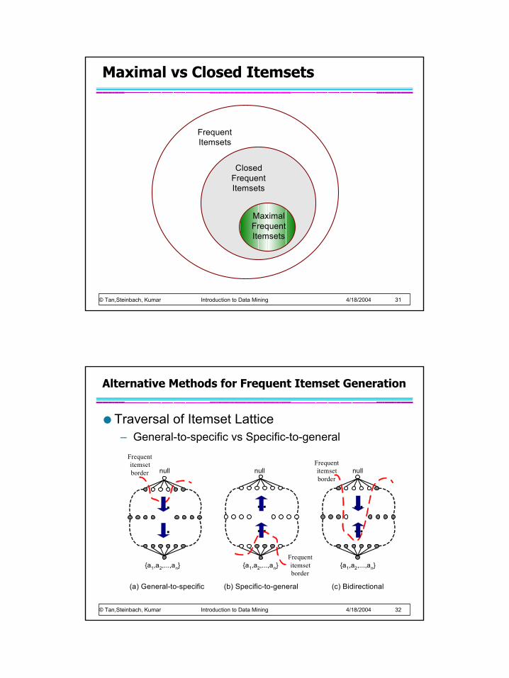
Maximal vs Closed Itemsets
FrequentItemsets
ClosedFrequentItemsets
MaximalFrequentItemsets
© Tan,Steinbach, Kumar Introduction to Data Mining 4/18/2004 32
Alternative Methods for Frequent Itemset Generation
Traversal of Itemset Lattice– General-to-specific vs Specific-to-general
Frequentitemsetborder null
{a1,a2,...,an}
(a) General-to-specific
null
{a1,a2,...,an}
Frequentitemsetborder
(b) Specific-to-general
..
......
Frequentitemsetborder
null
{a1,a2,...,an}
(c) Bidirectional
..
..
Page 17
© Tan,Steinbach, Kumar Introduction to Data Mining 4/18/2004 33
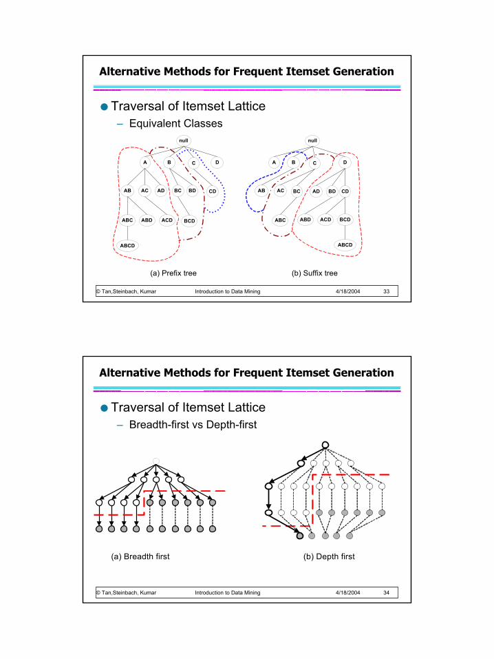
Alternative Methods for Frequent Itemset Generation
Traversal of Itemset Lattice– Equivalent Classes
null
AB AC AD BC BD CD
A B C D
ABC ABD ACD BCD
ABCD
null
AB AC ADBC BD CD
A B C D
ABC ABD ACD BCD
ABCD
(a) Prefix tree (b) Suffix tree
© Tan,Steinbach, Kumar Introduction to Data Mining 4/18/2004 34
Alternative Methods for Frequent Itemset Generation
Traversal of Itemset Lattice– Breadth-first vs Depth-first
(a) Breadth first (b) Depth first
Page 18
© Tan,Steinbach, Kumar Introduction to Data Mining 4/18/2004 35
Alternative Methods for Frequent Itemset Generation
Representation of Database– horizontal vs vertical data layout
TID Items1 A,B,E2 B,C,D3 C,E4 A,C,D5 A,B,C,D6 A,E7 A,B8 A,B,C9 A,C,D
10 B
HorizontalData Layout
A B C D E1 1 2 2 14 2 3 4 35 5 4 5 66 7 8 97 8 98 109
Vertical Data Layout
© Tan,Steinbach, Kumar Introduction to Data Mining 4/18/2004 36
FP-growth Algorithm
Use a compressed representation of the database using an FP-tree
Once an FP-tree has been constructed, it uses a recursive divide-and-conquer approach to mine the frequent itemsets
Page 19
© Tan,Steinbach, Kumar Introduction to Data Mining 4/18/2004 37
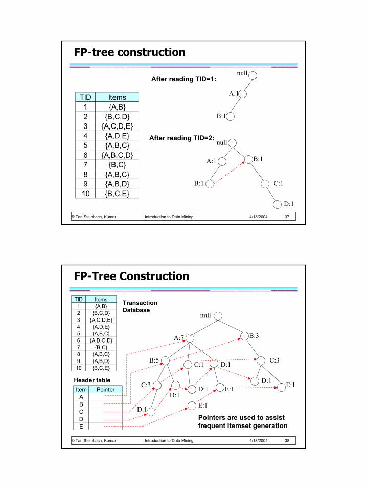
FP-tree construction
TID Items1 {A,B}2 {B,C,D}3 {A,C,D,E}4 {A,D,E}5 {A,B,C}6 {A,B,C,D}7 {B,C}8 {A,B,C}9 {A,B,D}10 {B,C,E}
null
A:1
B:1
null
A:1
B:1
B:1
C:1
D:1
After reading TID=1:
After reading TID=2:
© Tan,Steinbach, Kumar Introduction to Data Mining 4/18/2004 38
FP-Tree Construction
null
A:7
B:5
B:3
C:3
D:1
C:1
D:1C:3
D:1
D:1
E:1 E:1
TID Items1 {A,B}2 {B,C,D}3 {A,C,D,E}4 {A,D,E}5 {A,B,C}6 {A,B,C,D}7 {B,C}8 {A,B,C}9 {A,B,D}10 {B,C,E}
Pointers are used to assist frequent itemset generation
D:1E:1
Transaction Database
Item PointerABCDE
Header table
Page 20
© Tan,Steinbach, Kumar Introduction to Data Mining 4/18/2004 39
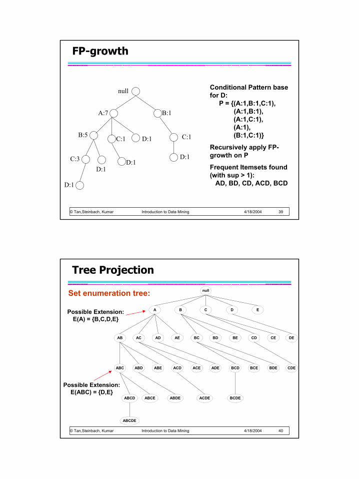
FP-growth
null
A:7
B:5
B:1
C:1
D:1
C:1
D:1C:3
D:1
D:1
Conditional Pattern base for D:
P = {(A:1,B:1,C:1),(A:1,B:1), (A:1,C:1),(A:1), (B:1,C:1)}
Recursively apply FP-growth on P
Frequent Itemsets found (with sup > 1):
AD, BD, CD, ACD, BCD
D:1
© Tan,Steinbach, Kumar Introduction to Data Mining 4/18/2004 40
Tree Projection
Set enumeration tree: null
AB AC AD AE BC BD BE CD CE DE
A B C D E
ABC ABD ABE ACD ACE ADE BCD BCE BDE CDE
ABCD ABCE ABDE ACDE BCDE
ABCDE
Possible Extension: E(A) = {B,C,D,E}
Possible Extension: E(ABC) = {D,E}
Page 21
© Tan,Steinbach, Kumar Introduction to Data Mining 4/18/2004 41
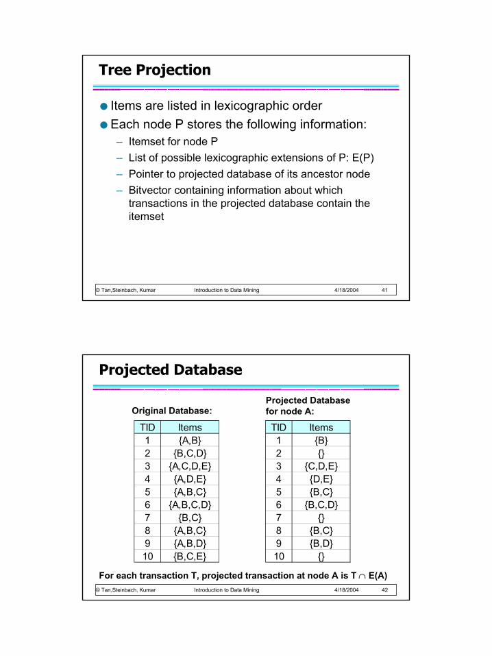
Tree Projection
Items are listed in lexicographic orderEach node P stores the following information:– Itemset for node P– List of possible lexicographic extensions of P: E(P)– Pointer to projected database of its ancestor node– Bitvector containing information about which
transactions in the projected database contain the itemset
© Tan,Steinbach, Kumar Introduction to Data Mining 4/18/2004 42
Projected Database
TID Items1 {A,B}2 {B,C,D}3 {A,C,D,E}4 {A,D,E}5 {A,B,C}6 {A,B,C,D}7 {B,C}8 {A,B,C}9 {A,B,D}10 {B,C,E}
TID Items1 {B}2 {}3 {C,D,E}4 {D,E}5 {B,C}6 {B,C,D}7 {}8 {B,C}9 {B,D}10 {}
Original Database:Projected Database for node A:
For each transaction T, projected transaction at node A is T ∩ E(A)
Page 22
© Tan,Steinbach, Kumar Introduction to Data Mining 4/18/2004 43
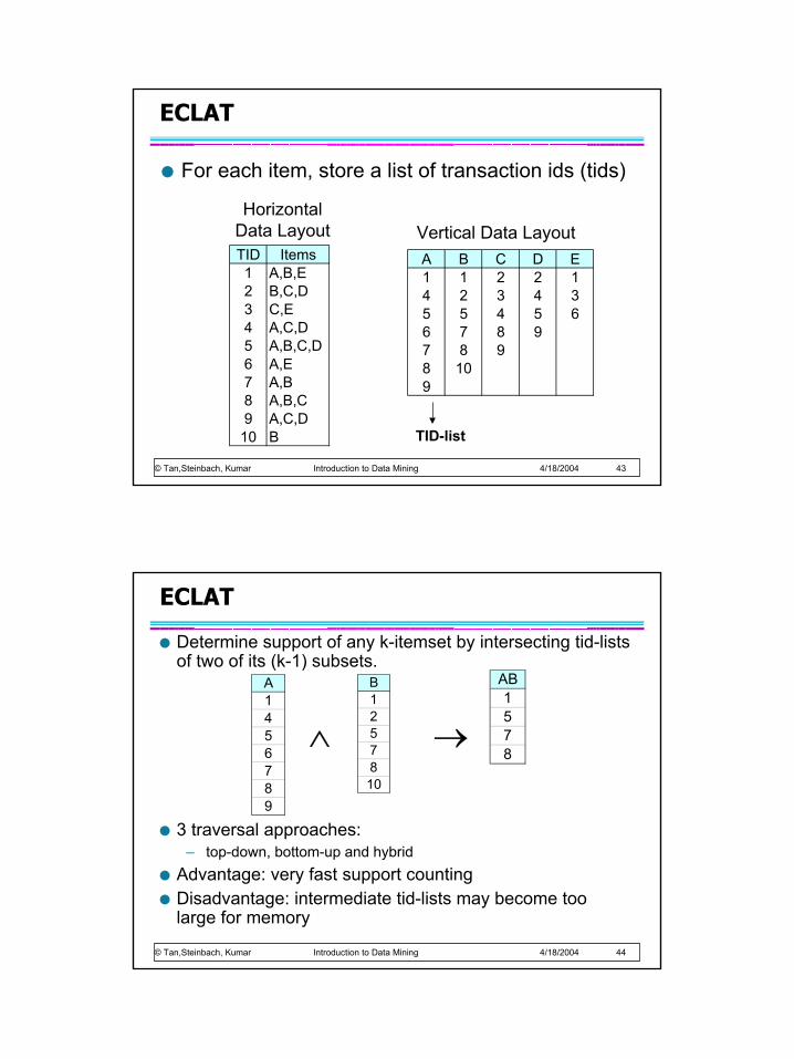
ECLAT
For each item, store a list of transaction ids (tids)
TID Items1 A,B,E2 B,C,D3 C,E4 A,C,D5 A,B,C,D6 A,E7 A,B8 A,B,C9 A,C,D
10 B
HorizontalData Layout
A B C D E1 1 2 2 14 2 3 4 35 5 4 5 66 7 8 97 8 98 109
Vertical Data Layout
TID-list
© Tan,Steinbach, Kumar Introduction to Data Mining 4/18/2004 44
ECLAT
Determine support of any k-itemset by intersecting tid-lists of two of its (k-1) subsets.
3 traversal approaches: – top-down, bottom-up and hybrid
Advantage: very fast support countingDisadvantage: intermediate tid-lists may become too large for memory
A1456789
B1257810
∧ →
AB1578
Page 23
© Tan,Steinbach, Kumar Introduction to Data Mining 4/18/2004 45
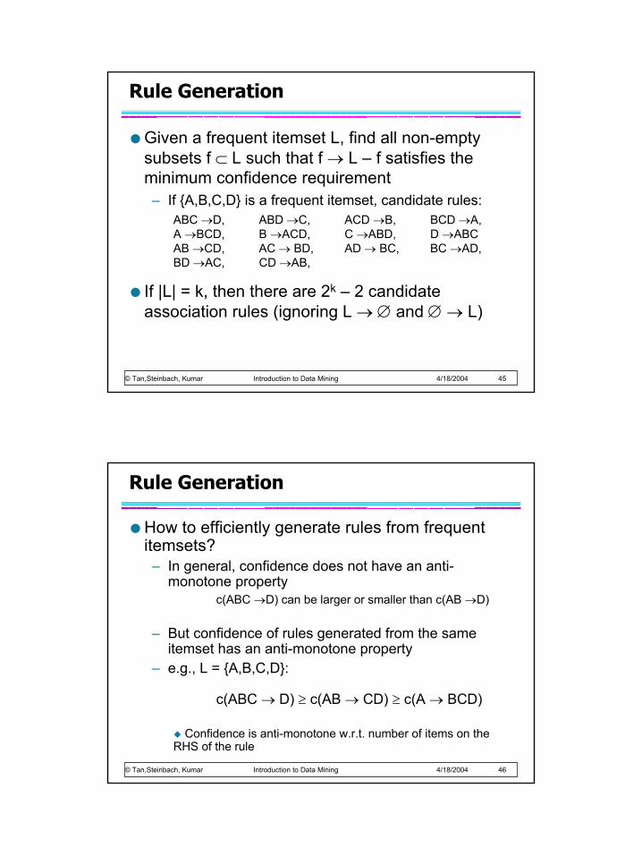
Rule Generation
Given a frequent itemset L, find all non-empty subsets f ⊂ L such that f → L – f satisfies the minimum confidence requirement– If {A,B,C,D} is a frequent itemset, candidate rules:
ABC →D, ABD →C, ACD →B, BCD →A, A →BCD, B →ACD, C →ABD, D →ABCAB →CD, AC → BD, AD → BC, BC →AD, BD →AC, CD →AB,
If |L| = k, then there are 2k – 2 candidate association rules (ignoring L → ∅ and ∅ → L)
© Tan,Steinbach, Kumar Introduction to Data Mining 4/18/2004 46
Rule Generation
How to efficiently generate rules from frequent itemsets?– In general, confidence does not have an anti-
monotone propertyc(ABC →D) can be larger or smaller than c(AB →D)
– But confidence of rules generated from the same itemset has an anti-monotone property
– e.g., L = {A,B,C,D}:
c(ABC → D) ≥ c(AB → CD) ≥ c(A → BCD)
Confidence is anti-monotone w.r.t. number of items on the RHS of the rule
Page 24
© Tan,Steinbach, Kumar Introduction to Data Mining 4/18/2004 47
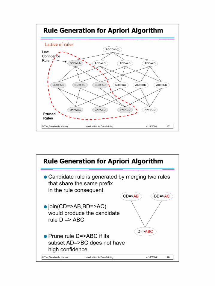
Rule Generation for Apriori Algorithm
ABCD=>{ }
BCD=>A ACD=>B ABD=>C ABC=>D
BC=>ADBD=>ACCD=>AB AD=>BC AC=>BD AB=>CD
D=>ABC C=>ABD B=>ACD A=>BCD
Lattice of rulesABCD=>{ }
BCD=>A ACD=>B ABD=>C ABC=>D
BC=>ADBD=>ACCD=>AB AD=>BC AC=>BD AB=>CD
D=>ABC C=>ABD B=>ACD A=>BCDPruned Rules
Low Confidence Rule
© Tan,Steinbach, Kumar Introduction to Data Mining 4/18/2004 48
Rule Generation for Apriori Algorithm
Candidate rule is generated by merging two rules that share the same prefixin the rule consequent
join(CD=>AB,BD=>AC)would produce the candidaterule D => ABC
Prune rule D=>ABC if itssubset AD=>BC does not havehigh confidence
BD=>ACCD=>AB
D=>ABC
Page 25
© Tan,Steinbach, Kumar Introduction to Data Mining 4/18/2004 49
Effect of Support Distribution
Many real data sets have skewed support distribution
Support distribution of a retail data set
© Tan,Steinbach, Kumar Introduction to Data Mining 4/18/2004 50
Effect of Support Distribution
How to set the appropriate minsup threshold?– If minsup is set too high, we could miss itemsets
involving interesting rare items (e.g., expensive products)
– If minsup is set too low, it is computationally expensive and the number of itemsets is very large
Using a single minimum support threshold may not be effective
Page 26
© Tan,Steinbach, Kumar Introduction to Data Mining 4/18/2004 51
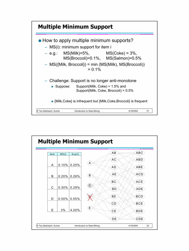
Multiple Minimum Support
How to apply multiple minimum supports?– MS(i): minimum support for item i – e.g.: MS(Milk)=5%, MS(Coke) = 3%,
MS(Broccoli)=0.1%, MS(Salmon)=0.5%– MS({Milk, Broccoli}) = min (MS(Milk), MS(Broccoli))
= 0.1%
– Challenge: Support is no longer anti-monotoneSuppose: Support(Milk, Coke) = 1.5% and
Support(Milk, Coke, Broccoli) = 0.5%
{Milk,Coke} is infrequent but {Milk,Coke,Broccoli} is frequent
© Tan,Steinbach, Kumar Introduction to Data Mining 4/18/2004 52
Multiple Minimum Support
A
Item MS(I) Sup(I)
A 0.10% 0.25%
B 0.20% 0.26%
C 0.30% 0.29%
D 0.50% 0.05%
E 3% 4.20%
B
C
D
E
AB
AC
AD
AE
BC
BD
BE
CD
CE
DE
ABC
ABD
ABE
ACD
ACE
ADE
BCD
BCE
BDE
CDE
Page 27
© Tan,Steinbach, Kumar Introduction to Data Mining 4/18/2004 53
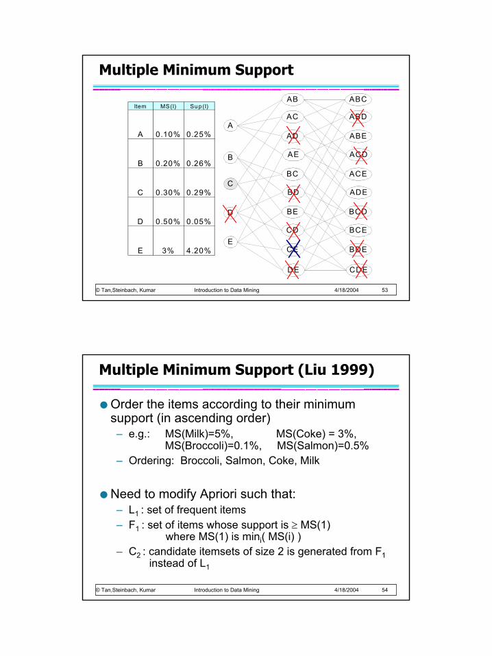
Multiple Minimum Support
A
B
C
D
E
AB
AC
AD
AE
BC
BD
BE
CD
CE
DE
ABC
ABD
ABE
ACD
ACE
ADE
BCD
BCE
BDE
CDE
Item MS(I) Sup(I)
A 0.10% 0.25%
B 0.20% 0.26%
C 0.30% 0.29%
D 0.50% 0.05%
E 3% 4.20%
© Tan,Steinbach, Kumar Introduction to Data Mining 4/18/2004 54
Multiple Minimum Support (Liu 1999)
Order the items according to their minimum support (in ascending order)– e.g.: MS(Milk)=5%, MS(Coke) = 3%,
MS(Broccoli)=0.1%, MS(Salmon)=0.5%– Ordering: Broccoli, Salmon, Coke, Milk
Need to modify Apriori such that:– L1 : set of frequent items– F1 : set of items whose support is ≥ MS(1)
where MS(1) is mini( MS(i) )– C2 : candidate itemsets of size 2 is generated from F1
instead of L1
Page 28
© Tan,Steinbach, Kumar Introduction to Data Mining 4/18/2004 55
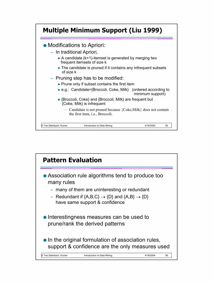
Multiple Minimum Support (Liu 1999)
Modifications to Apriori:– In traditional Apriori,
A candidate (k+1)-itemset is generated by merging twofrequent itemsets of size kThe candidate is pruned if it contains any infrequent subsetsof size k
– Pruning step has to be modified:Prune only if subset contains the first iteme.g.: Candidate={Broccoli, Coke, Milk} (ordered according to
minimum support){Broccoli, Coke} and {Broccoli, Milk} are frequent but {Coke, Milk} is infrequent
– Candidate is not pruned because {Coke,Milk} does not containthe first item, i.e., Broccoli.
© Tan,Steinbach, Kumar Introduction to Data Mining 4/18/2004 56
Pattern Evaluation
Association rule algorithms tend to produce too many rules – many of them are uninteresting or redundant– Redundant if {A,B,C} → {D} and {A,B} → {D}
have same support & confidence
Interestingness measures can be used to prune/rank the derived patterns
In the original formulation of association rules, support & confidence are the only measures used
Page 29
© Tan,Steinbach, Kumar Introduction to Data Mining 4/18/2004 57
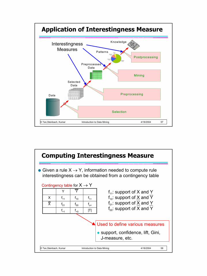
Application of Interestingness Measure
Feature
Product
Product
Product
Product
Product
Product
Product
Product
Product
Product
FeatureFeatureFeatureFeatureFeatureFeatureFeatureFeatureFeature
Selection
Preprocessing
Mining
Postprocessing
Data
SelectedData
PreprocessedData
Patterns
KnowledgeInterestingness Measures
© Tan,Steinbach, Kumar Introduction to Data Mining 4/18/2004 58
Computing Interestingness Measure
Given a rule X → Y, information needed to compute rule interestingness can be obtained from a contingency table
|T|f+0f+1
fo+f00f01X
f1+f10f11X
Y Y
Contingency table for X → Yf11: support of X and Yf10: support of X and Yf01: support of X and Yf00: support of X and Y
Used to define various measures
support, confidence, lift, Gini,J-measure, etc.
Page 30
© Tan,Steinbach, Kumar Introduction to Data Mining 4/18/2004 59
Drawback of Confidence
100109080575Tea20515Tea
CoffeeCoffee
Association Rule: Tea → Coffee
Confidence= P(Coffee|Tea) = 0.75
but P(Coffee) = 0.9
⇒ Although confidence is high, rule is misleading
⇒ P(Coffee|Tea) = 0.9375
© Tan,Steinbach, Kumar Introduction to Data Mining 4/18/2004 60
Statistical Independence
Population of 1000 students– 600 students know how to swim (S)– 700 students know how to bike (B)– 420 students know how to swim and bike (S,B)
– P(S∧B) = 420/1000 = 0.42– P(S) × P(B) = 0.6 × 0.7 = 0.42
– P(S∧B) = P(S) × P(B) => Statistical independence– P(S∧B) > P(S) × P(B) => Positively correlated– P(S∧B) < P(S) × P(B) => Negatively correlated
Page 31
© Tan,Steinbach, Kumar Introduction to Data Mining 4/18/2004 61
Statistical-based Measures
Measures that take into account statistical dependence
)](1)[()](1)[()()(),(
)()(),()()(
),()(
)|(
YPYPXPXPYPXPYXPtcoefficien
YPXPYXPPSYPXPYXPInterest
YPXYPLift
−−−
=−
−=
=
=
φ
© Tan,Steinbach, Kumar Introduction to Data Mining 4/18/2004 62
Example: Lift/Interest
100109080575Tea20515Tea
CoffeeCoffee
Association Rule: Tea → Coffee
Confidence= P(Coffee|Tea) = 0.75
but P(Coffee) = 0.9
⇒ Lift = 0.75/0.9= 0.8333 (< 1, therefore is negatively associated)
Page 32
© Tan,Steinbach, Kumar Introduction to Data Mining 4/18/2004 63
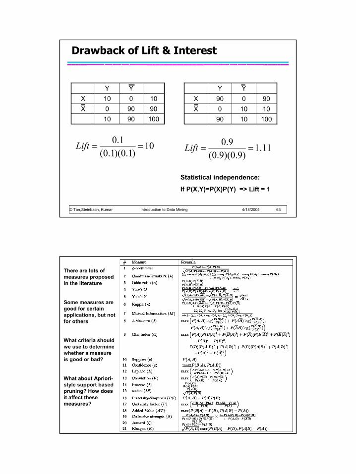
Drawback of Lift & Interest
100901090900X10010X
YY
100109010100X90090X
YY
10)1.0)(1.0(
1.0==Lift 11.1
)9.0)(9.0(9.0
==Lift
Statistical independence:
If P(X,Y)=P(X)P(Y) => Lift = 1
There are lots of measures proposed in the literature
Some measures are good for certain applications, but not for others
What criteria should we use to determine whether a measure is good or bad?
What about Apriori-style support based pruning? How does it affect these measures?
Page 33
© Tan,Steinbach, Kumar Introduction to Data Mining 4/18/2004 65
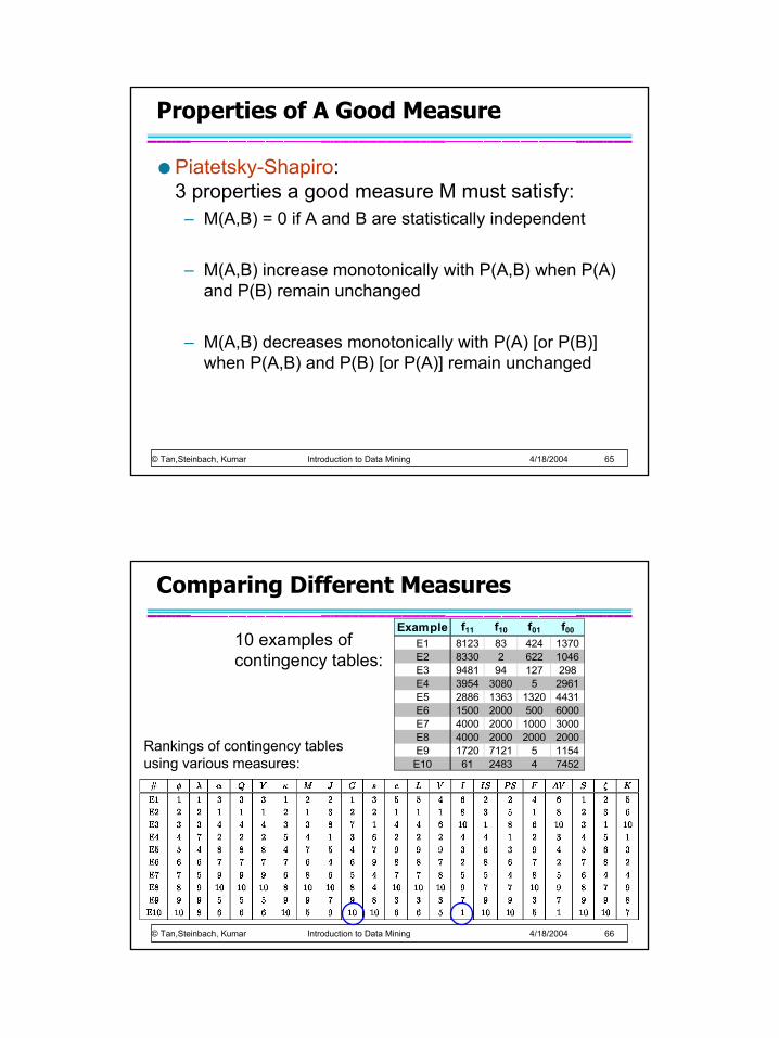
Properties of A Good Measure
Piatetsky-Shapiro: 3 properties a good measure M must satisfy:– M(A,B) = 0 if A and B are statistically independent
– M(A,B) increase monotonically with P(A,B) when P(A) and P(B) remain unchanged
– M(A,B) decreases monotonically with P(A) [or P(B)] when P(A,B) and P(B) [or P(A)] remain unchanged
© Tan,Steinbach, Kumar Introduction to Data Mining 4/18/2004 66
Comparing Different Measures
Example f11 f10 f01 f00
E1 8123 83 424 1370E2 8330 2 622 1046E3 9481 94 127 298E4 3954 3080 5 2961E5 2886 1363 1320 4431E6 1500 2000 500 6000E7 4000 2000 1000 3000E8 4000 2000 2000 2000E9 1720 7121 5 1154
E10 61 2483 4 7452
10 examples of contingency tables:
Rankings of contingency tables using various measures:
Page 34
© Tan,Steinbach, Kumar Introduction to Data Mining 4/18/2004 67
Property under Variable Permutation
B B A p q A r s
A A B p r B q s
Does M(A,B) = M(B,A)?
Symmetric measures:
support, lift, collective strength, cosine, Jaccard, etc
Asymmetric measures:
confidence, conviction, Laplace, J-measure, etc
© Tan,Steinbach, Kumar Introduction to Data Mining 4/18/2004 68
Property under Row/Column Scaling
1073
541Low
532High
FemaleMale
76706
42402Low
34304High
FemaleMale
Grade-Gender Example (Mosteller, 1968):
Mosteller: Underlying association should be independent ofthe relative number of male and female studentsin the samples
2x 10x
Page 35
© Tan,Steinbach, Kumar Introduction to Data Mining 4/18/2004 69
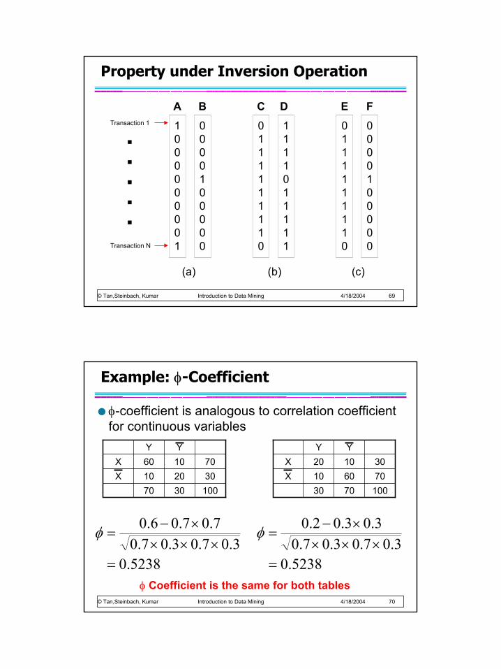
Property under Inversion Operation
1000000001
0000100000
0111111110
1111011111
A B C D
(a) (b)
0111111110
0000100000
(c)
E FTransaction 1
Transaction N
.
.
.
.
.
© Tan,Steinbach, Kumar Introduction to Data Mining 4/18/2004 70
Example: φ-Coefficient
φ-coefficient is analogous to correlation coefficient for continuous variables
1003070302010X701060X
YY
1007030706010X301020X
YY
5238.03.07.03.07.0
7.07.06.0
=×××
×−=φ
φ Coefficient is the same for both tables
5238.03.07.03.07.0
3.03.02.0
=×××
×−=φ
Page 36
© Tan,Steinbach, Kumar Introduction to Data Mining 4/18/2004 71
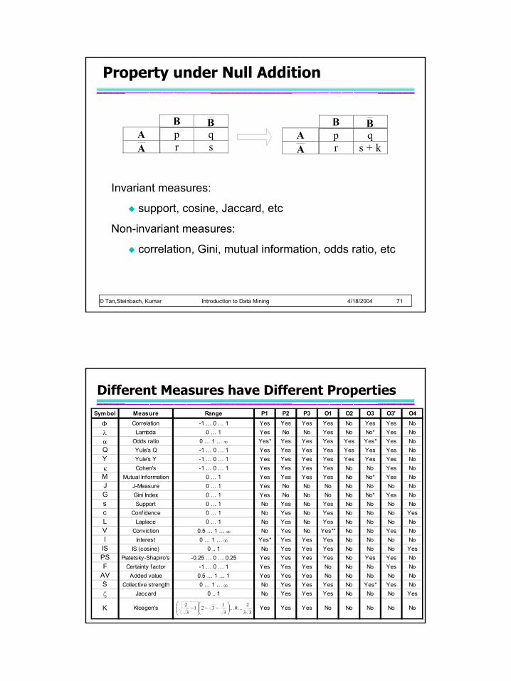
Property under Null Addition
B B A p q A r s
B B A p q A r s + k
Invariant measures:
support, cosine, Jaccard, etc
Non-invariant measures:
correlation, Gini, mutual information, odds ratio, etc
© Tan,Steinbach, Kumar Introduction to Data Mining 4/18/2004 72
Different Measures have Different PropertiesSymbol Measure Range P1 P2 P3 O1 O2 O3 O3' O4
Φ Correlation -1 … 0 … 1 Yes Yes Yes Yes No Yes Yes Noλ Lambda 0 … 1 Yes No No Yes No No* Yes Noα Odds ratio 0 … 1 … ∞ Yes* Yes Yes Yes Yes Yes* Yes NoQ Yule's Q -1 … 0 … 1 Yes Yes Yes Yes Yes Yes Yes NoY Yule's Y -1 … 0 … 1 Yes Yes Yes Yes Yes Yes Yes Noκ Cohen's -1 … 0 … 1 Yes Yes Yes Yes No No Yes NoM Mutual Information 0 … 1 Yes Yes Yes Yes No No* Yes NoJ J-Measure 0 … 1 Yes No No No No No No NoG Gini Index 0 … 1 Yes No No No No No* Yes Nos Support 0 … 1 No Yes No Yes No No No Noc Confidence 0 … 1 No Yes No Yes No No No YesL Laplace 0 … 1 No Yes No Yes No No No NoV Conviction 0.5 … 1 … ∞ No Yes No Yes** No No Yes NoI Interest 0 … 1 … ∞ Yes* Yes Yes Yes No No No No
IS IS (cosine) 0 .. 1 No Yes Yes Yes No No No YesPS Piatetsky-Shapiro's -0.25 … 0 … 0.25 Yes Yes Yes Yes No Yes Yes NoF Certainty factor -1 … 0 … 1 Yes Yes Yes No No No Yes No
AV Added value 0.5 … 1 … 1 Yes Yes Yes No No No No NoS Collective strength 0 … 1 … ∞ No Yes Yes Yes No Yes* Yes Noζ Jaccard 0 .. 1 No Yes Yes Yes No No No Yes
K Klosgen's Yes Yes Yes No No No No No33
203
13213
2KK
−−
−
Page 37
© Tan,Steinbach, Kumar Introduction to Data Mining 4/18/2004 73
Support-based Pruning
Most of the association rule mining algorithms use support measure to prune rules and itemsets
Study effect of support pruning on correlation of itemsets– Generate 10000 random contingency tables– Compute support and pairwise correlation for each
table– Apply support-based pruning and examine the tables
that are removed
© Tan,Steinbach, Kumar Introduction to Data Mining 4/18/2004 74
Effect of Support-based Pruning
All Itempairs
0
100
200
300
400
500
600
700
800
900
1000
-1-0.
9-0.
8-0.
7-0.
6-0.
5-0.
4-0.
3-0.
2-0.
1 00.1 0.2 0.3 0.4 0.5 0.6 0.7 0.8 0.9
1
Correlation
Page 38
© Tan,Steinbach, Kumar Introduction to Data Mining 4/18/2004 75
Effect of Support-based PruningSupport < 0.01
0
50
100
150
200
250
300
-1 -0.9
-0.8
-0.7
-0.6
-0.5
-0.4
-0.3
-0.2
-0.1 0 0.1 0.2 0.3 0.4 0.5 0.6 0.7 0.8 0.9 1
Correlation
Support < 0.03
0
50
100
150
200
250
300
-1 -0.9
-0.8
-0.7
-0.6
-0.5
-0.4
-0.3
-0.2
-0.1 0 0.1 0.2 0.3 0.4 0.5 0.6 0.7 0.8 0.9 1
Correlation
Support < 0.05
0
50
100
150
200
250
300
-1 -0.9
-0.8
-0.7
-0.6
-0.5
-0.4
-0.3
-0.2
-0.1 0 0.1 0.2 0.3 0.4 0.5 0.6 0.7 0.8 0.9 1
Correlation
Support-based pruning eliminates mostly negatively correlated itemsets
© Tan,Steinbach, Kumar Introduction to Data Mining 4/18/2004 76
Effect of Support-based Pruning
Investigate how support-based pruning affects other measures
Steps:– Generate 10000 contingency tables– Rank each table according to the different measures– Compute the pair-wise correlation between the
measures
Page 39
© Tan,Steinbach, Kumar Introduction to Data Mining 4/18/2004 77
Effect of Support-based Pruning
All P a irs (4 0 .14% )
1 2 3 4 5 6 7 8 9 10 11 12 13 14 15 16 17 18 19 20 21
C onviction
Odds ratio
Col S treng th
C orrelation
Interes t
PS
C F
Yule Y
Reliability
Kappa
Klos g en
Yule Q
C onfidence
Laplace
IS
Support
J accard
Lambda
Gini
J -meas ure
Mutual Info
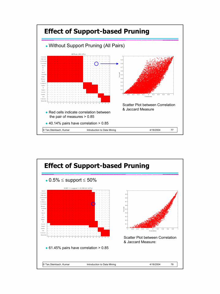
Without Support Pruning (All Pairs)
Red cells indicate correlation betweenthe pair of measures > 0.85
40.14% pairs have correlation > 0.85
-1 -0.8 -0.6 -0.4 -0.2 0 0.2 0.4 0.6 0.8 10
0.1
0.2
0.3
0.4
0.5
0.6
0.7
0.8
0.9
1
Corre la tion
Jacc
ard
Scatter Plot between Correlation & Jaccard Measure
© Tan,Steinbach, Kumar Introduction to Data Mining 4/18/2004 78
Effect of Support-based Pruning
0.5% ≤ support ≤ 50%
61.45% pairs have correlation > 0.85
0 .00 5 <= s upp ort <= 0 .5 00 (61 .45 % )
1 2 3 4 5 6 7 8 9 10 11 12 13 14 15 16 17 18 19 20 21
Interes t
C onviction
Odds ratio
Col S treng th
Laplace
C onfidence
C orrelation
Klos g en
Reliability
PS
Yule Q
C F
Yule Y
Kappa
IS
J accard
Support
Lambda
Gini
J -meas ure
Mutual Info
-1 -0.8 -0.6 -0.4 -0.2 0 0.2 0.4 0.6 0.8 10
0.1
0.2
0.3
0.4
0.5
0.6
0.7
0.8
0.9
1
Corre la tion
Jacc
ard
Scatter Plot between Correlation & Jaccard Measure:
Page 40
© Tan,Steinbach, Kumar Introduction to Data Mining 4/18/2004 79
0 .00 5 <= s upp ort <= 0 .3 00 (76 .42 % )
1 2 3 4 5 6 7 8 9 10 11 12 13 14 15 16 17 18 19 20 21
Support
Interes t
Reliability
C onviction
Yule Q
Odds ratio
C onfidence
C F
Yule Y
Kappa
C orrelation
Col S treng th
IS
J accard
Laplace
PS
Klos g en
Lambda
Mutual Info
Gini
J -meas ure
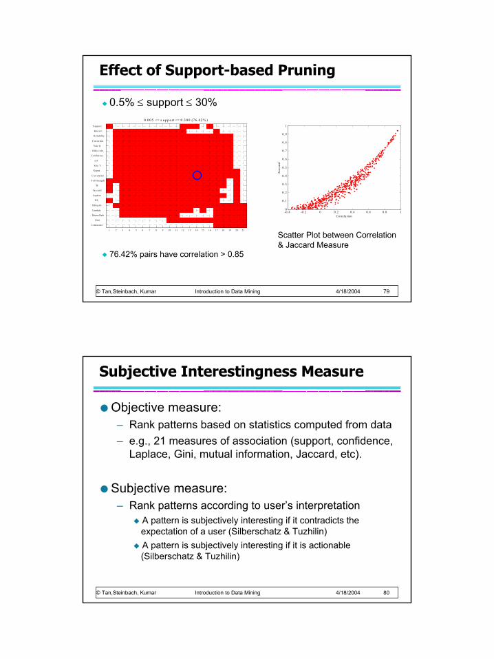
Effect of Support-based Pruning
0.5% ≤ support ≤ 30%
76.42% pairs have correlation > 0.85
-0.4 -0.2 0 0.2 0.4 0.6 0.8 10
0.1
0.2
0.3
0.4
0.5
0.6
0.7
0.8
0.9
1
Corre la tion
Jacc
ard
Scatter Plot between Correlation & Jaccard Measure
© Tan,Steinbach, Kumar Introduction to Data Mining 4/18/2004 80
Subjective Interestingness Measure
Objective measure: – Rank patterns based on statistics computed from data– e.g., 21 measures of association (support, confidence,
Laplace, Gini, mutual information, Jaccard, etc).
Subjective measure:– Rank patterns according to user’s interpretation
A pattern is subjectively interesting if it contradicts theexpectation of a user (Silberschatz & Tuzhilin)A pattern is subjectively interesting if it is actionable(Silberschatz & Tuzhilin)
Page 41
© Tan,Steinbach, Kumar Introduction to Data Mining 4/18/2004 81
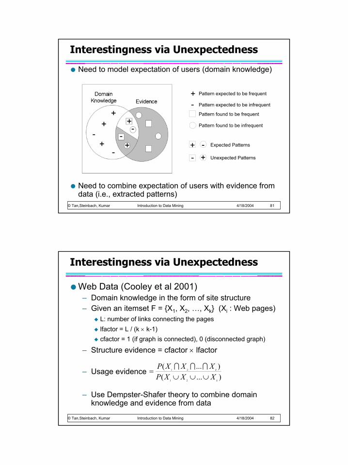
Interestingness via Unexpectedness
Need to model expectation of users (domain knowledge)
Need to combine expectation of users with evidence from data (i.e., extracted patterns)
+ Pattern expected to be frequent
- Pattern expected to be infrequent
Pattern found to be frequent
Pattern found to be infrequent
+-
Expected Patterns-+ Unexpected Patterns
© Tan,Steinbach, Kumar Introduction to Data Mining 4/18/2004 82
Interestingness via Unexpectedness
Web Data (Cooley et al 2001)– Domain knowledge in the form of site structure– Given an itemset F = {X1, X2, …, Xk} (Xi : Web pages)
L: number of links connecting the pages lfactor = L / (k × k-1)cfactor = 1 (if graph is connected), 0 (disconnected graph)
– Structure evidence = cfactor × lfactor
– Usage evidence
– Use Dempster-Shafer theory to combine domain knowledge and evidence from data
)...()...(
21
21
k
k
XXXPXXXP
∪∪∪=
III