Lecture Notes for Chapter 4 Introduction to Data Mining by Tan, Steinbach, Kumar (modified by Predrag Radivojac, 2017) Data Mining Classification: Basic Concepts, Decision Trees, and Model Evaluation
Transcript
Lecture Notes for Chapter 4
Introduction to Data Miningby
Tan, Steinbach, Kumar
(modified by Predrag Radivojac, 2017)
Data Mining Classification: Basic Concepts, Decision
Trees, and Model Evaluation
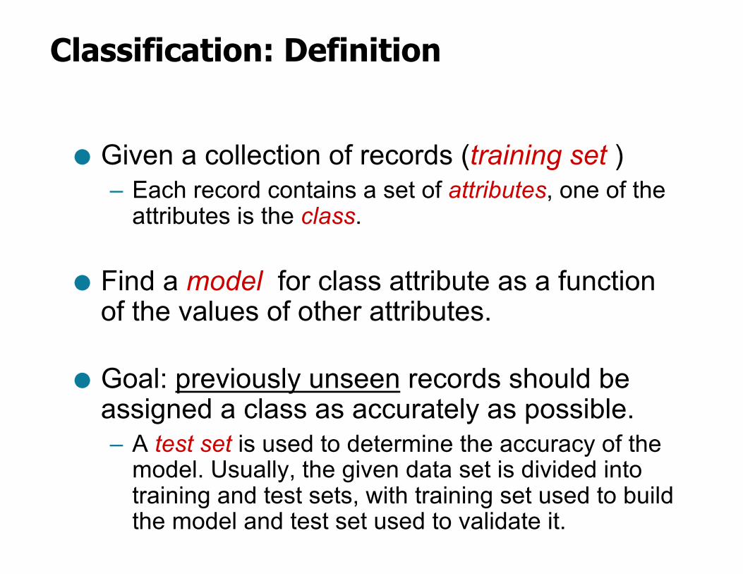
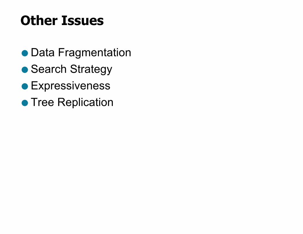
Classification: Definition
● Given a collection of records (training set )– Each record contains a set of attributes, one of the
attributes is the class.
● Find a model for class attribute as a function of the values of other attributes.
● Goal: previously unseen records should be assigned a class as accurately as possible.– A test set is used to determine the accuracy of the
model. Usually, the given data set is divided into training and test sets, with training set used to build the model and test set used to validate it.
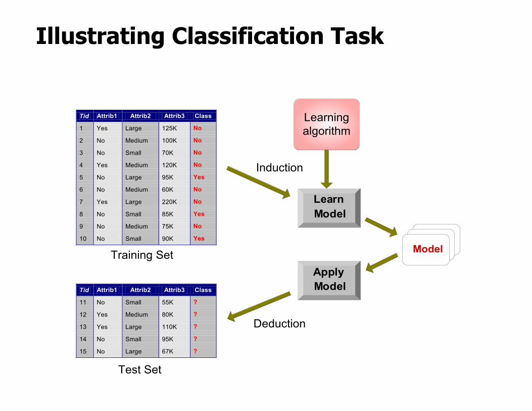
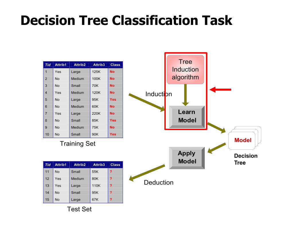
Illustrating Classification Task
Apply Model
Induction
Deduction
Learn Model
Model
Tid Attrib1 Attrib2 Attrib3 Class
1 Yes Large 125K No
2 No Medium 100K No
3 No Small 70K No
4 Yes Medium 120K No
5 No Large 95K Yes
6 No Medium 60K No
7 Yes Large 220K No
8 No Small 85K Yes
9 No Medium 75K No
10 No Small 90K Yes 10
Tid Attrib1 Attrib2 Attrib3 Class
11 No Small 55K ?
12 Yes Medium 80K ?
13 Yes Large 110K ?
14 No Small 95K ?
15 No Large 67K ? 10
Test Set
Learningalgorithm
Training Set
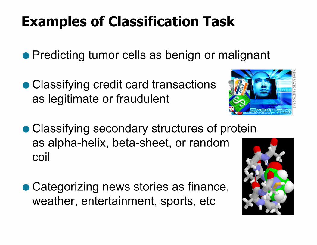
Examples of Classification Task
● Predicting tumor cells as benign or malignant
● Classifying credit card transactions as legitimate or fraudulent
● Classifying secondary structures of protein as alpha-helix, beta-sheet, or random coil
● Categorizing news stories as finance, weather, entertainment, sports, etc
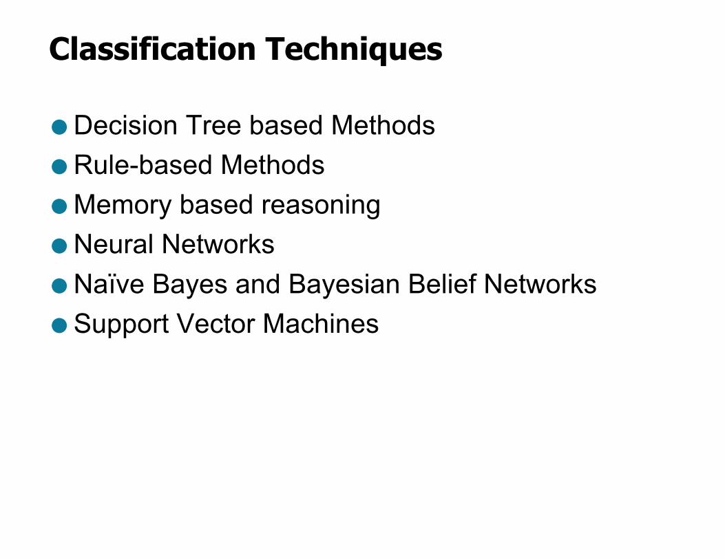
Classification Techniques
● Decision Tree based Methods● Rule-based Methods● Memory based reasoning● Neural Networks● Naïve Bayes and Bayesian Belief Networks● Support Vector Machines
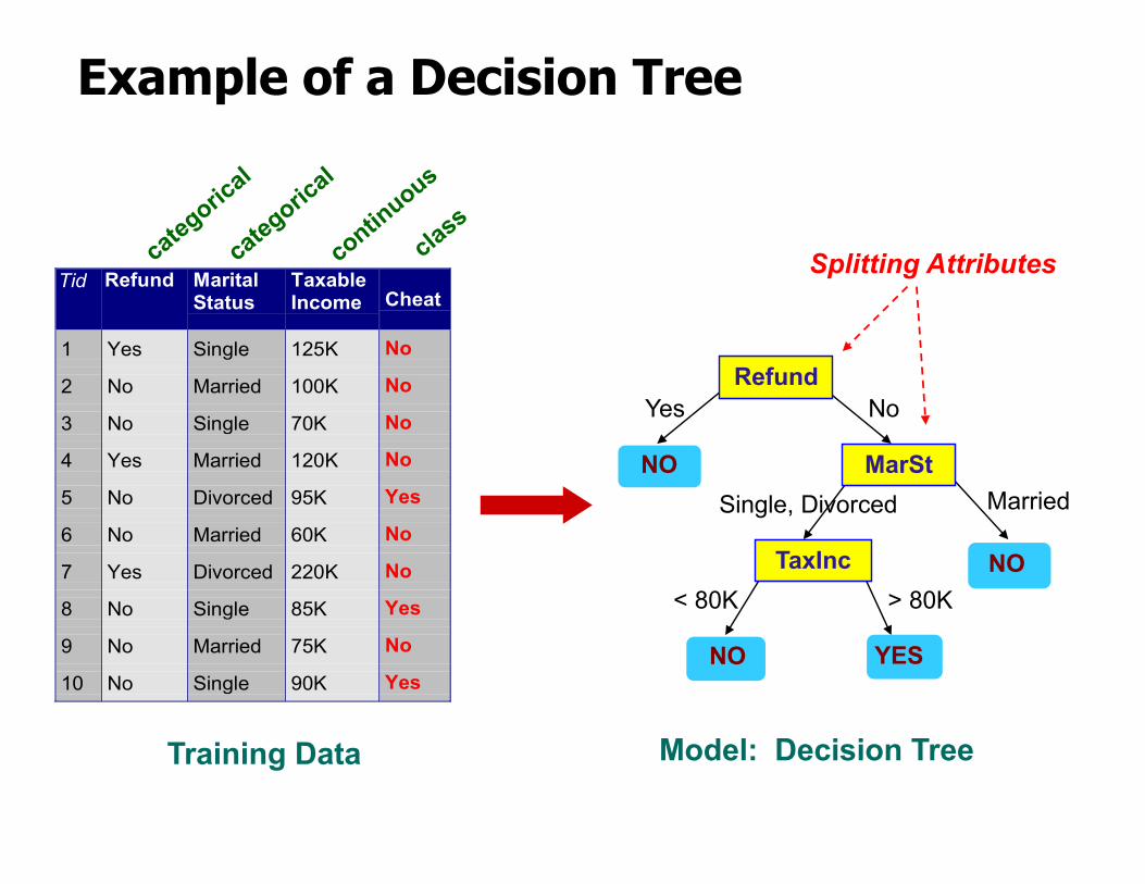
Example of a Decision Tree
Tid Refund MaritalStatus
TaxableIncome Cheat
1 Yes Single 125K No
2 No Married 100K No
3 No Single 70K No
4 Yes Married 120K No
5 No Divorced 95K Yes
6 No Married 60K No
7 Yes Divorced 220K No
8 No Single 85K Yes
9 No Married 75K No
10 No Single 90K Yes10
Refund
MarSt
TaxInc
YESNO
NO
NO
Yes No
MarriedSingle, Divorced
< 80K > 80K
Splitting Attributes
Training Data Model: Decision Tree
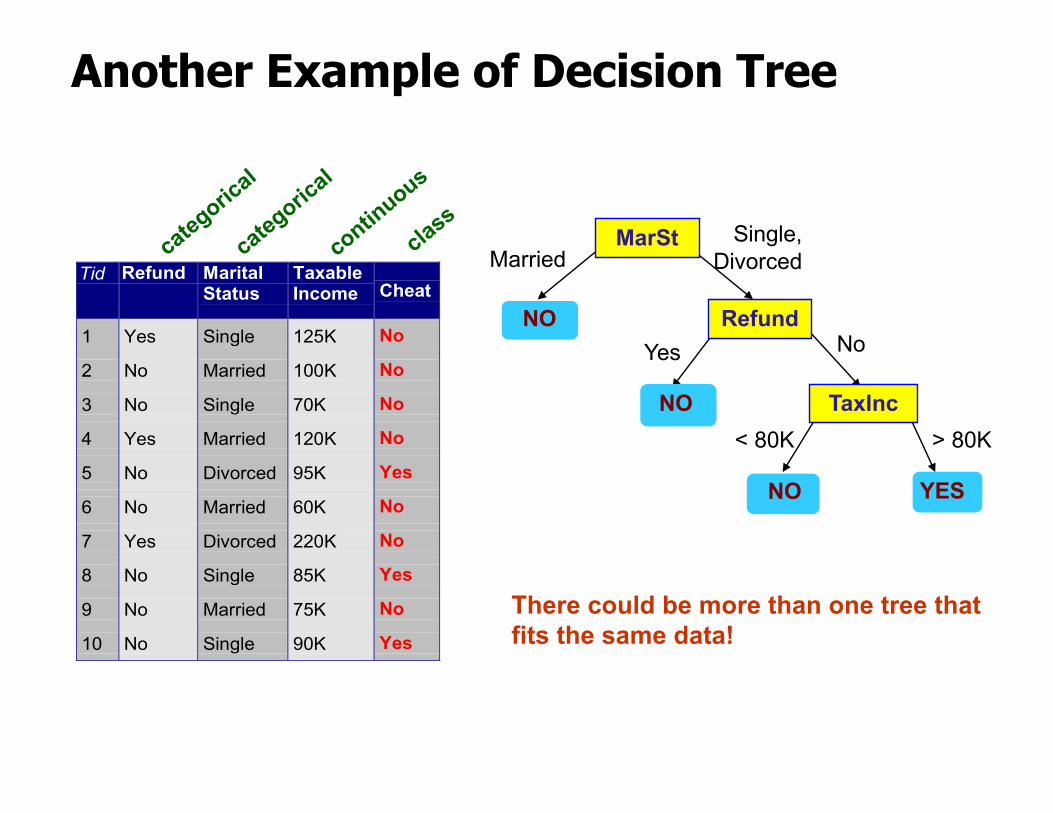
Another Example of Decision Tree
Tid Refund MaritalStatus
TaxableIncome Cheat
1 Yes Single 125K No
2 No Married 100K No
3 No Single 70K No
4 Yes Married 120K No
5 No Divorced 95K Yes
6 No Married 60K No
7 Yes Divorced 220K No
8 No Single 85K Yes
9 No Married 75K No
10 No Single 90K Yes10
MarSt
Refund
TaxInc
YESNO
NO
NO
Yes No
MarriedSingle,
Divorced
< 80K > 80K
There could be more than one tree that fits the same data!
Decision Tree Classification Task
Apply Model
Induction
Deduction
Learn Model
Model
Tid Attrib1 Attrib2 Attrib3 Class
1 Yes Large 125K No
2 No Medium 100K No
3 No Small 70K No
4 Yes Medium 120K No
5 No Large 95K Yes
6 No Medium 60K No
7 Yes Large 220K No
8 No Small 85K Yes
9 No Medium 75K No
10 No Small 90K Yes 10
Tid Attrib1 Attrib2 Attrib3 Class
11 No Small 55K ?
12 Yes Medium 80K ?
13 Yes Large 110K ?
14 No Small 95K ?
15 No Large 67K ? 10
Test Set
TreeInductionalgorithm
Training SetDecision Tree
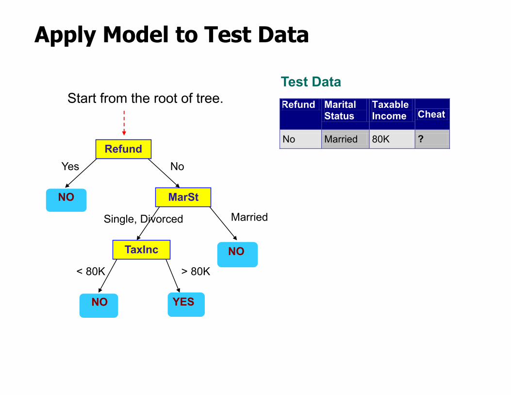
Apply Model to Test Data
Refund
MarSt
TaxInc
YESNO
NO
NO
Yes No
MarriedSingle, Divorced
< 80K > 80K
Refund Marital Status
Taxable Income Cheat
No Married 80K ? 10
Test DataStart from the root of tree.
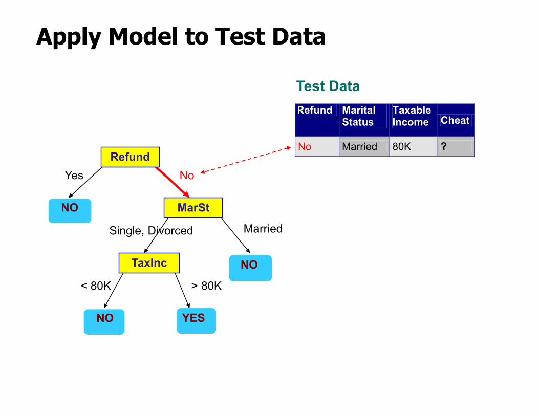
Apply Model to Test Data
Refund
MarSt
TaxInc
YESNO
NO
NO
Yes No
MarriedSingle, Divorced
< 80K > 80K
Refund Marital Status
Taxable Income Cheat
No Married 80K ? 10
Test Data
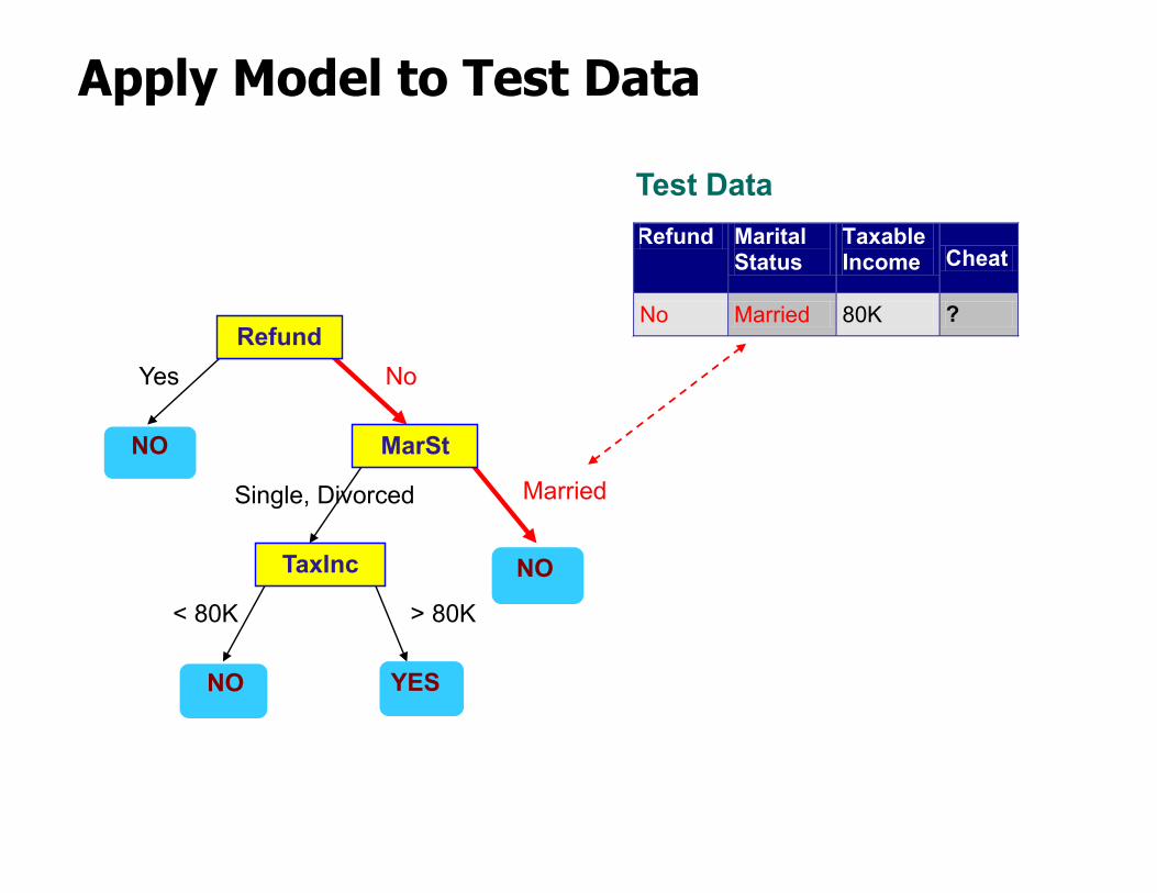
Apply Model to Test Data
Refund
MarSt
TaxInc
YESNO
NO
NO
Yes No
MarriedSingle, Divorced
< 80K > 80K
Refund Marital Status
Taxable Income Cheat
No Married 80K ? 10
Test Data
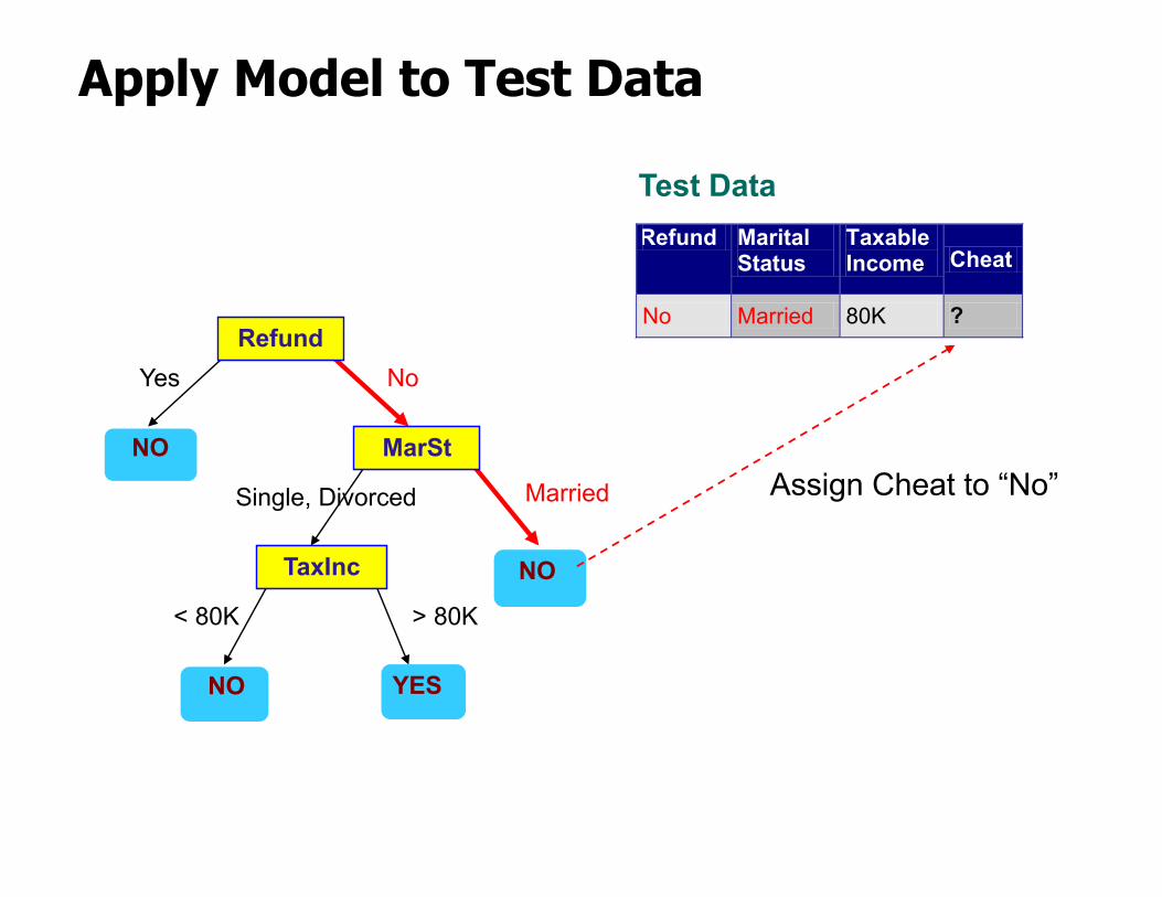
Apply Model to Test Data
Refund
MarSt
TaxInc
YESNO
NO
NO
Yes No
MarriedSingle, Divorced
< 80K > 80K
Refund Marital Status
Taxable Income Cheat
No Married 80K ? 10
Test Data
Apply Model to Test Data
Refund
MarSt
TaxInc
YESNO
NO
NO
Yes No
Married Single, Divorced
< 80K > 80K
Refund Marital Status
Taxable Income Cheat
No Married 80K ? 10
Test Data
Apply Model to Test Data
Refund
MarSt
TaxInc
YESNO
NO
NO
Yes No
Married Single, Divorced
< 80K > 80K
Refund Marital Status
Taxable Income Cheat
No Married 80K ? 10
Test Data
Assign Cheat to “No”
Decision Tree Classification Task
Apply Model
Induction
Deduction
Learn Model
Model
Tid Attrib1 Attrib2 Attrib3 Class
1 Yes Large 125K No
2 No Medium 100K No
3 No Small 70K No
4 Yes Medium 120K No
5 No Large 95K Yes
6 No Medium 60K No
7 Yes Large 220K No
8 No Small 85K Yes
9 No Medium 75K No
10 No Small 90K Yes 10
Tid Attrib1 Attrib2 Attrib3 Class
11 No Small 55K ?
12 Yes Medium 80K ?
13 Yes Large 110K ?
14 No Small 95K ?
15 No Large 67K ? 10
Test Set
TreeInductionalgorithm
Training Set
Decision Tree
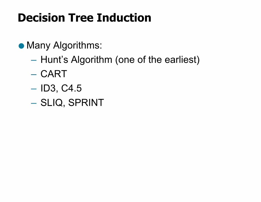
Decision Tree Induction
● Many Algorithms:– Hunt’s Algorithm (one of the earliest)– CART– ID3, C4.5– SLIQ, SPRINT
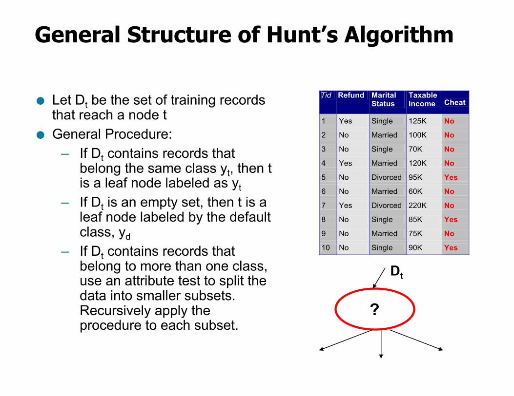
General Structure of Hunt’s Algorithm
● Let Dt be the set of training records that reach a node t
● General Procedure:– If Dt contains records that
belong the same class yt, then t is a leaf node labeled as yt
– If Dt is an empty set, then t is a leaf node labeled by the default class, yd
– If Dt contains records that belong to more than one class, use an attribute test to split the data into smaller subsets. Recursively apply the procedure to each subset.
Tid Refund Marital Status
Taxable Income Cheat
1 Yes Single 125K No
2 No Married 100K No
3 No Single 70K No
4 Yes Married 120K No
5 No Divorced 95K Yes
6 No Married 60K No
7 Yes Divorced 220K No
8 No Single 85K Yes
9 No Married 75K No
10 No Single 90K Yes 10
Dt
?
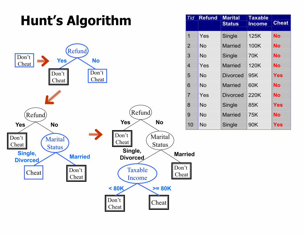
Hunt’s Algorithm
Don’t Cheat
Refund
Don’t Cheat
Don’t Cheat
Yes No
Refund
Don’t Cheat
Yes No
MaritalStatus
Don’t Cheat
Cheat
Single,Divorced Married
TaxableIncome
Don’t Cheat
< 80K >= 80K
Refund
Don’t Cheat
Yes No
MaritalStatus
Don’t Cheat
Cheat
Single,Divorced Married
Tid Refund MaritalStatus
TaxableIncome Cheat
1 Yes Single 125K No
2 No Married 100K No
3 No Single 70K No
4 Yes Married 120K No
5 No Divorced 95K Yes
6 No Married 60K No
7 Yes Divorced 220K No
8 No Single 85K Yes
9 No Married 75K No
10 No Single 90K Yes10
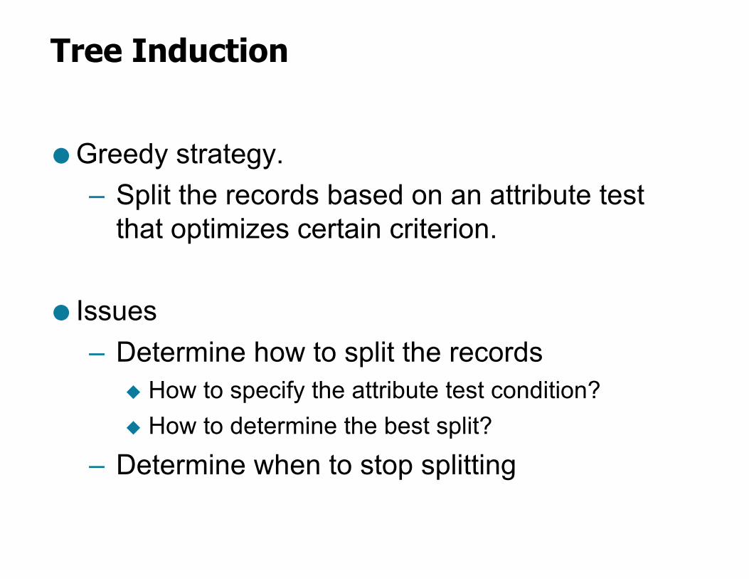
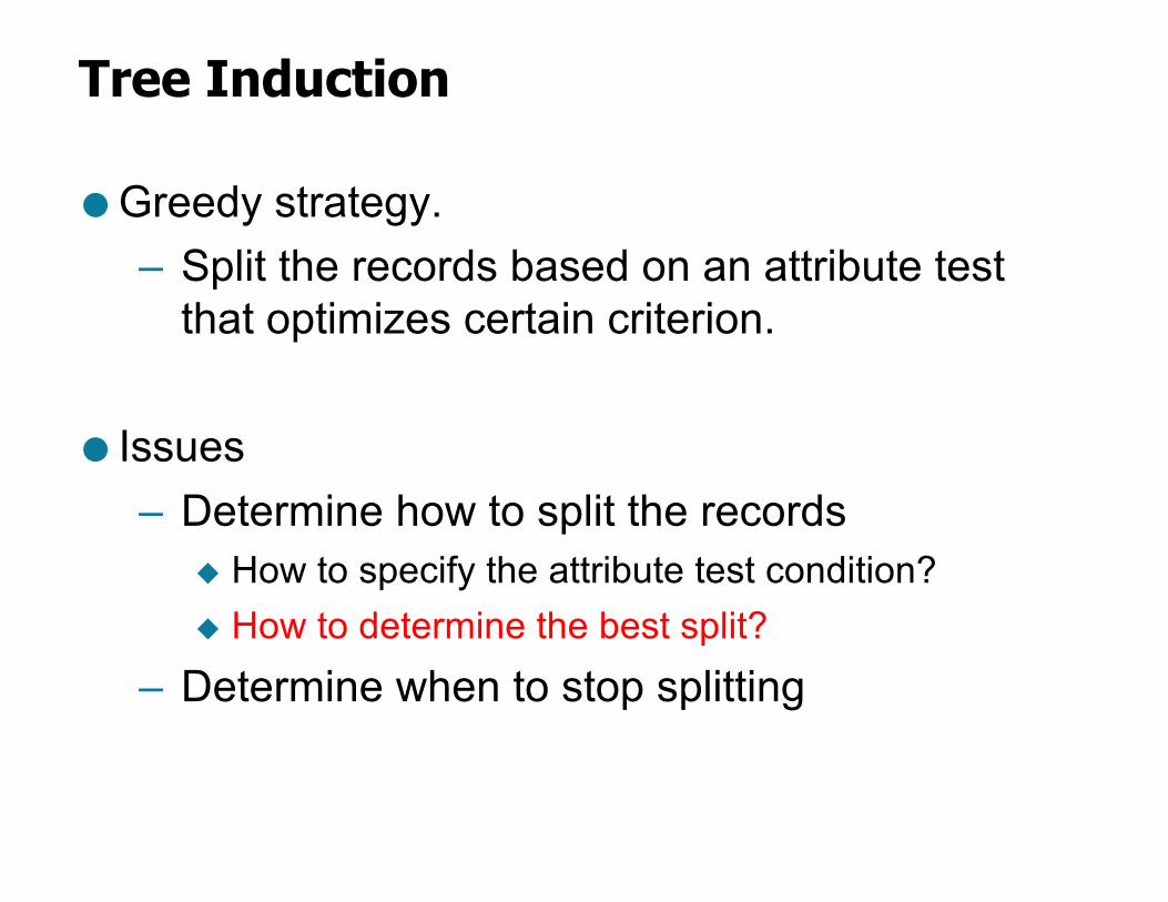
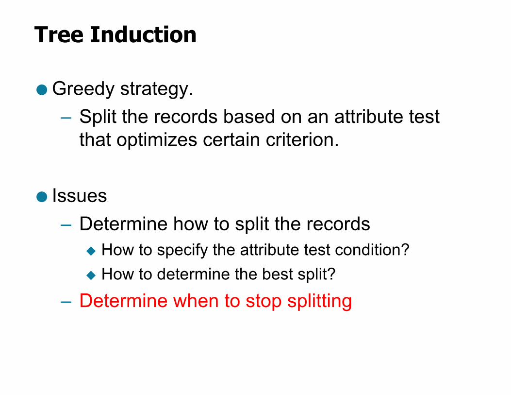
Tree Induction
● Greedy strategy.– Split the records based on an attribute test
that optimizes certain criterion.
● Issues– Determine how to split the records
u How to specify the attribute test condition?u How to determine the best split?
– Determine when to stop splitting
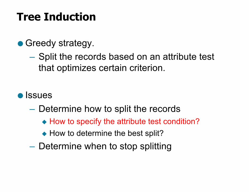
Tree Induction
● Greedy strategy.– Split the records based on an attribute test
that optimizes certain criterion.
● Issues– Determine how to split the records
u How to specify the attribute test condition?u How to determine the best split?
– Determine when to stop splitting
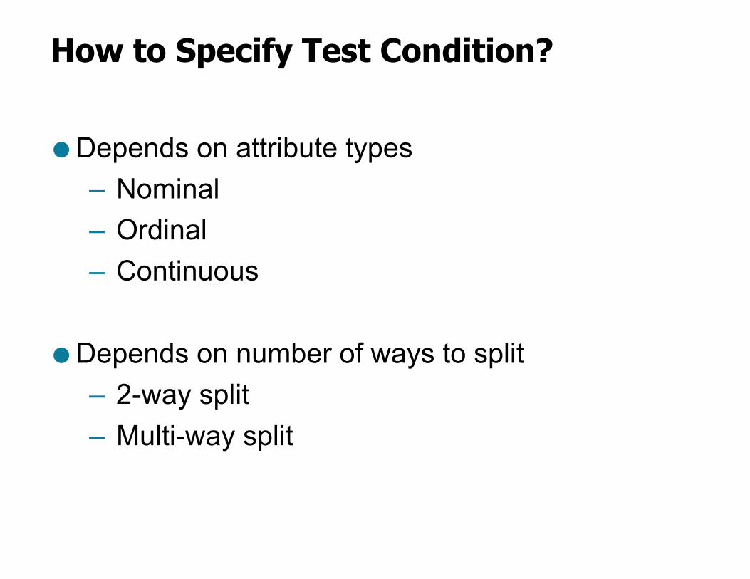
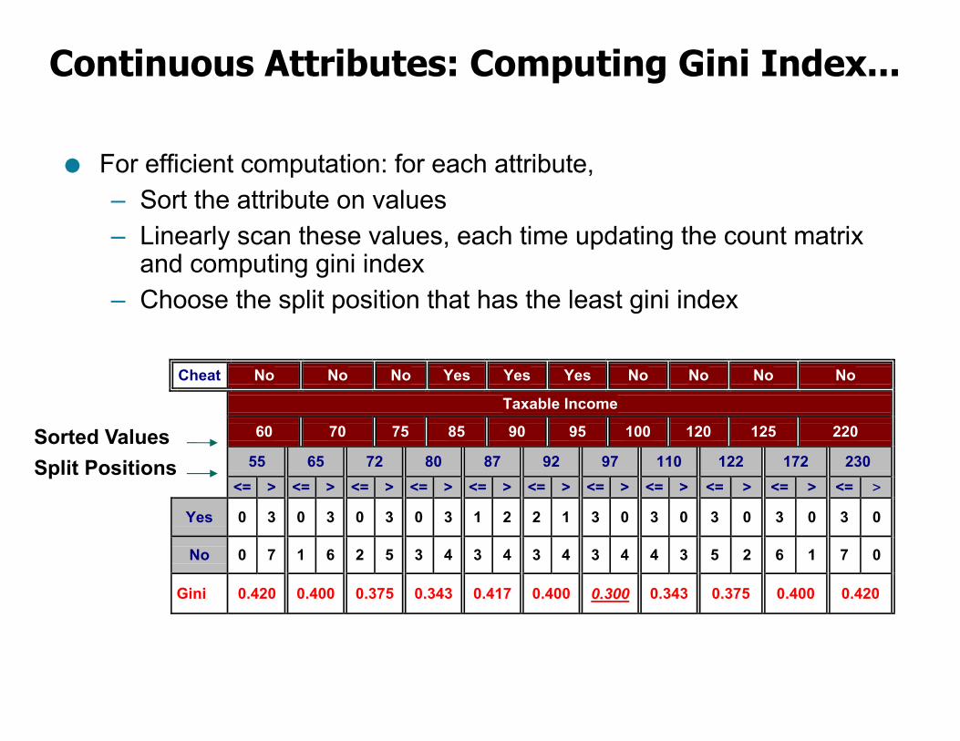
How to Specify Test Condition?
● Depends on attribute types– Nominal– Ordinal– Continuous
● Depends on number of ways to split– 2-way split– Multi-way split
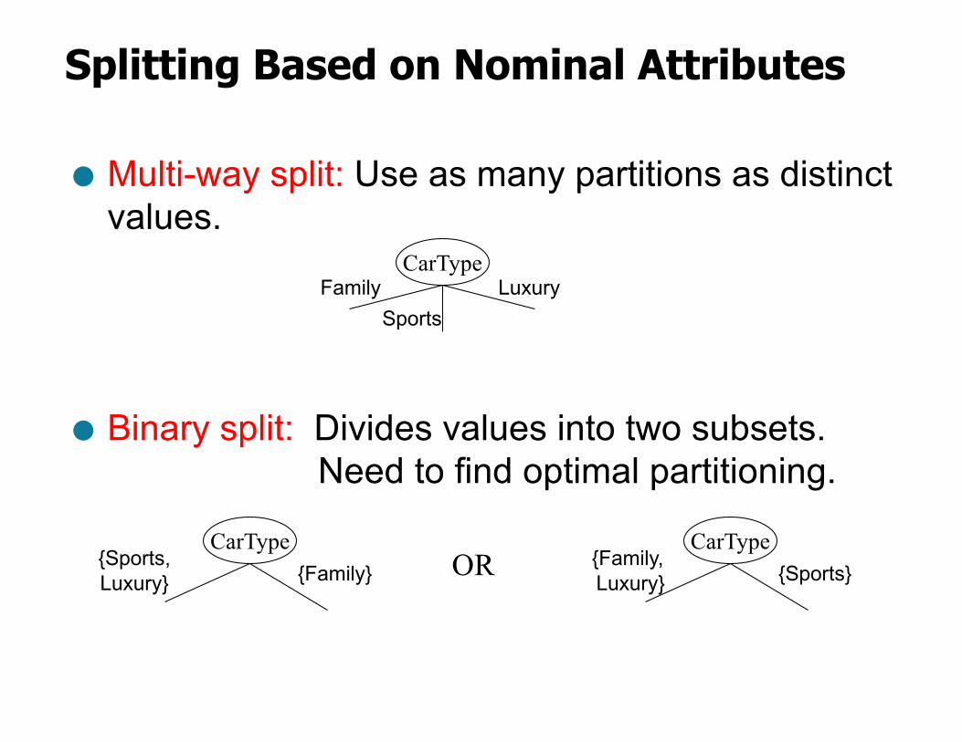
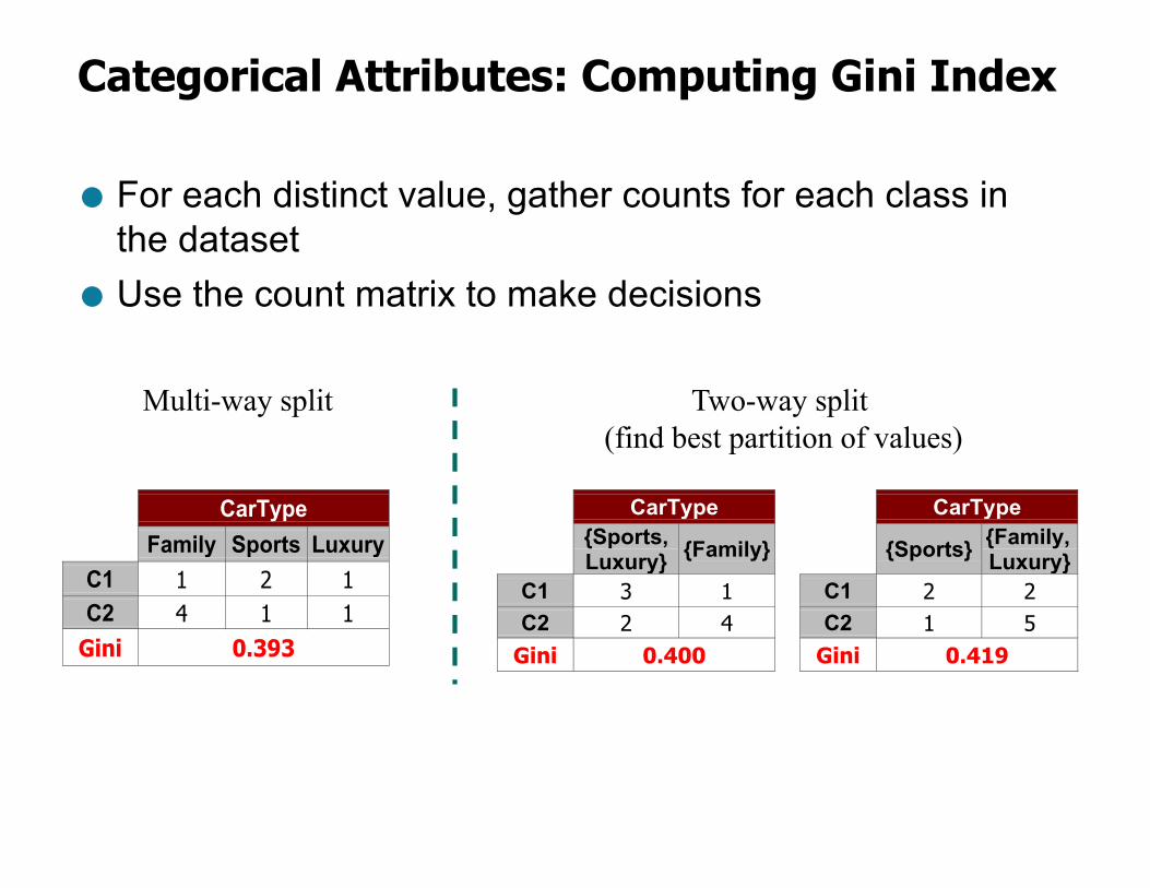
Splitting Based on Nominal Attributes
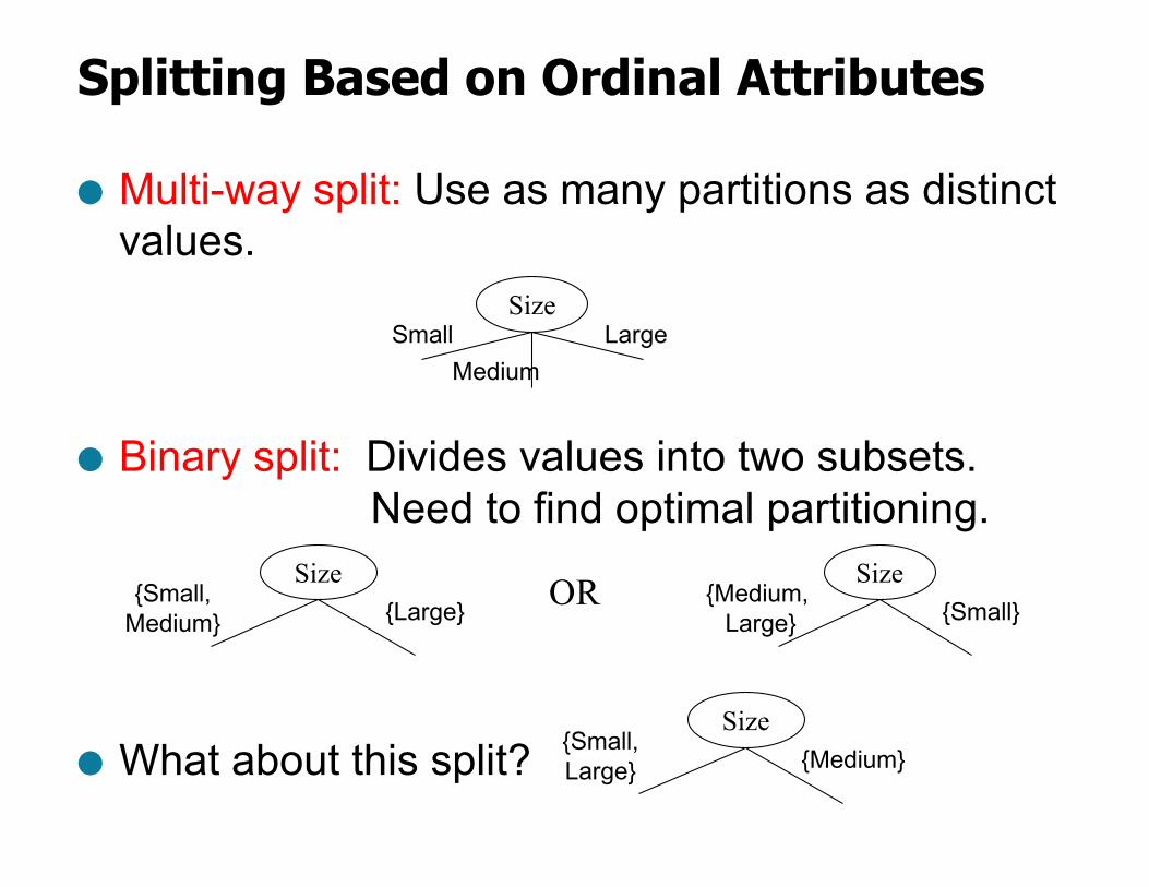
● Multi-way split: Use as many partitions as distinct values.
● Binary split: Divides values into two subsets. Need to find optimal partitioning.
CarTypeFamily
SportsLuxury
CarType{Family, Luxury} {Sports}
CarType{Sports, Luxury} {Family} OR
● Multi-way split: Use as many partitions as distinct values.
● Binary split: Divides values into two subsets. Need to find optimal partitioning.
● What about this split?
Splitting Based on Ordinal Attributes
SizeSmall
MediumLarge
Size{Medium,
Large} {Small}Size
{Small, Medium} {Large} OR
Size{Small, Large} {Medium}
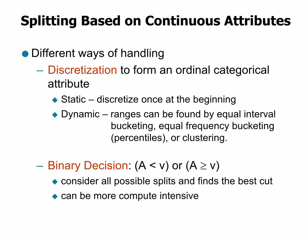
Splitting Based on Continuous Attributes
● Different ways of handling– Discretization to form an ordinal categorical
attributeu Static – discretize once at the beginningu Dynamic – ranges can be found by equal interval
bucketing, equal frequency bucketing(percentiles), or clustering.
– Binary Decision: (A < v) or (A ³ v)u consider all possible splits and finds the best cutu can be more compute intensive
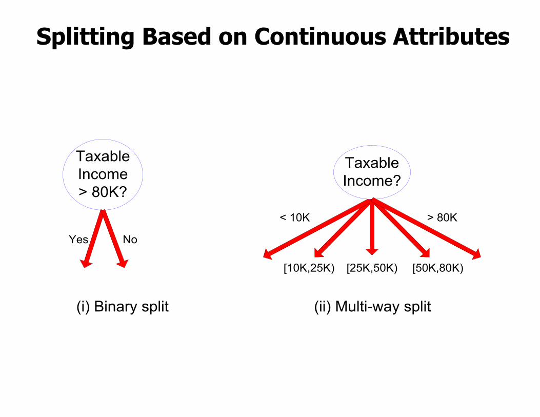
Splitting Based on Continuous Attributes
TaxableIncome> 80K?
Yes No
TaxableIncome?
(i) Binary split (ii) Multi-way split
< 10K
[10K,25K) [25K,50K) [50K,80K)
> 80K
Tree Induction
● Greedy strategy.– Split the records based on an attribute test
that optimizes certain criterion.
● Issues– Determine how to split the records
u How to specify the attribute test condition?u How to determine the best split?
– Determine when to stop splitting
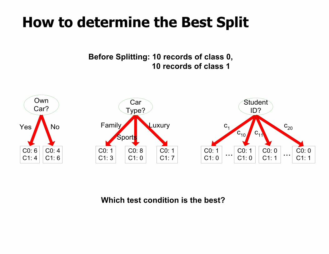
How to determine the Best Split
OwnCar?
C0: 6C1: 4
C0: 4C1: 6
C0: 1C1: 3
C0: 8C1: 0
C0: 1C1: 7
CarType?
C0: 1C1: 0
C0: 1C1: 0
C0: 0C1: 1
StudentID?
...
Yes No Family
Sports
Luxury c1 c10
c20
C0: 0C1: 1
...
c11
Before Splitting: 10 records of class 0,10 records of class 1
Which test condition is the best?
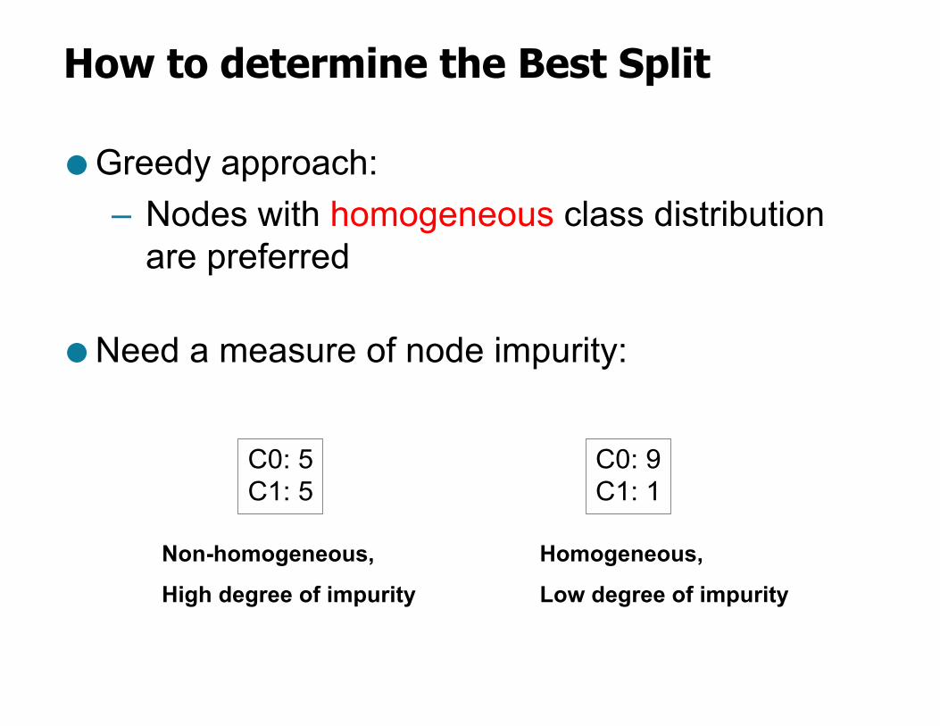
How to determine the Best Split
● Greedy approach: – Nodes with homogeneous class distribution
are preferred
● Need a measure of node impurity:
C0: 5C1: 5
C0: 9C1: 1
Non-homogeneous,
High degree of impurity
Homogeneous,
Low degree of impurity
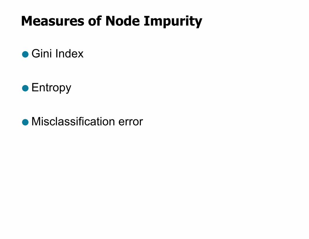
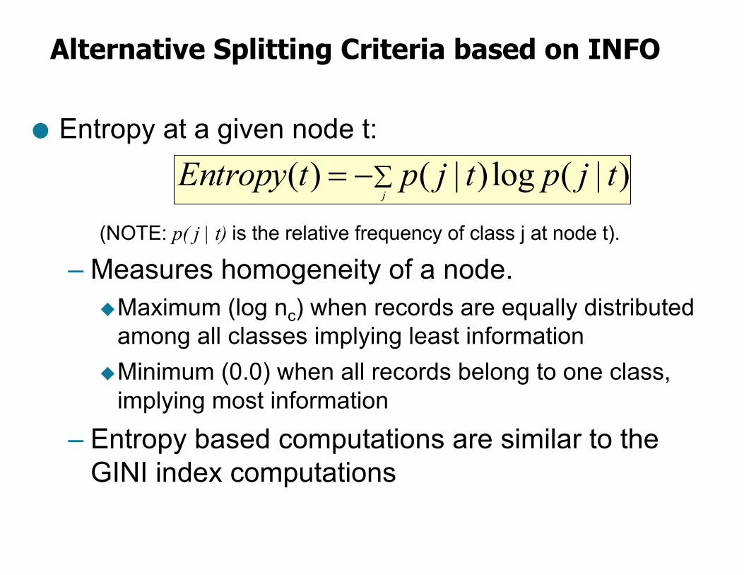
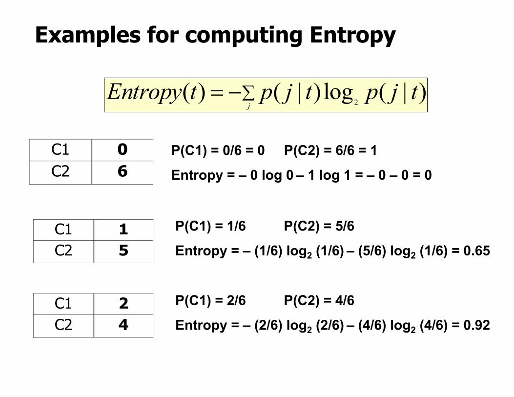
Measures of Node Impurity
● Gini Index
● Entropy
● Misclassification error
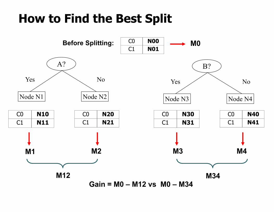
How to Find the Best Split
B?
Yes No
Node N3 Node N4
A?
Yes No
Node N1 Node N2
Before Splitting:
C0 N10 C1 N11
C0 N20 C1 N21
C0 N30 C1 N31
C0 N40 C1 N41
C0 N00 C1 N01
M0
M1 M2 M3 M4
M12 M34Gain = M0 – M12 vs M0 – M34
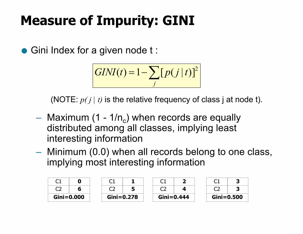
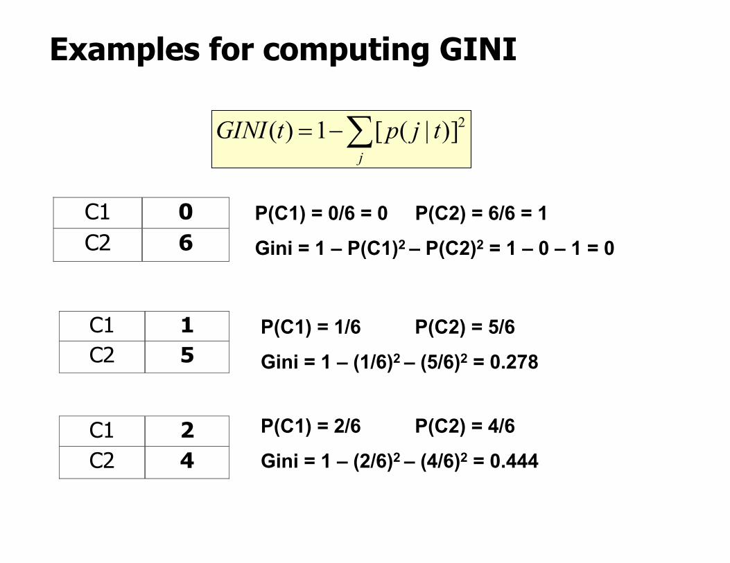
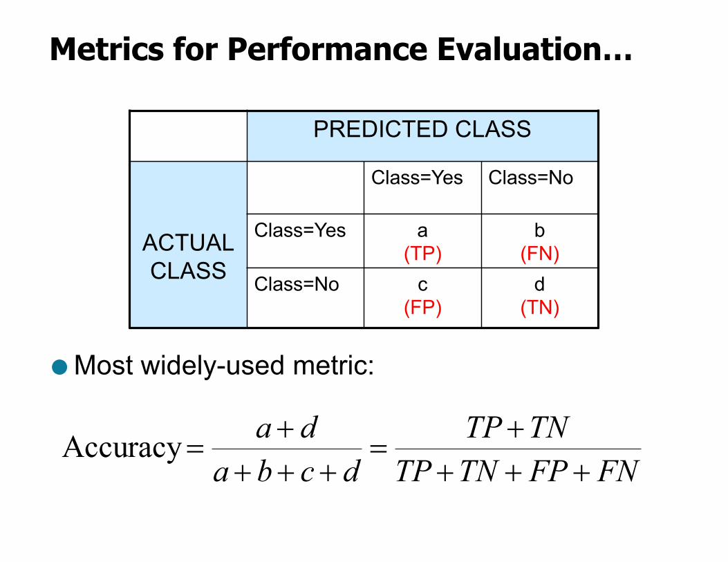
Measure of Impurity: GINI
● Gini Index for a given node t :
(NOTE: p( j | t) is the relative frequency of class j at node t).
– Maximum (1 - 1/nc) when records are equally distributed among all classes, implying least interesting information
– Minimum (0.0) when all records belong to one class, implying most interesting information
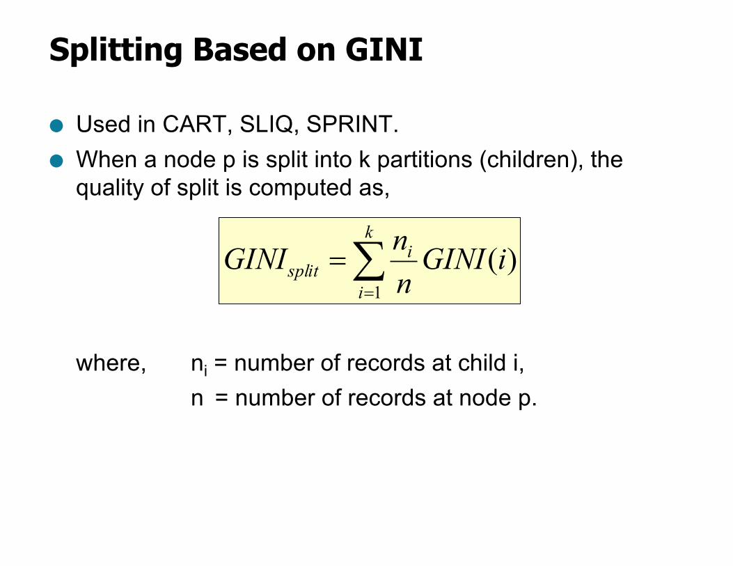
Parent Node, p is split into k partitions;ni is number of records in partition i
– Measures Reduction in Entropy achieved because of the split. Choose the split that achieves most reduction (maximizes GAIN)
– Used in ID3 and C4.5– Disadvantage: Tends to prefer splits that result in large
number of partitions, each being small but pure.
÷øö
çèæ-= å
=
k
i
i
splitiEntropy
nnpEntropyGAIN
1)()(
Splitting Based on INFO...
● Gain Ratio:
Parent Node, p is split into k partitionsni is the number of records in partition i
– Adjusts Information Gain by the entropy of the partitioning (SplitINFO). Higher entropy partitioning (large number of small partitions) is penalized!
– Used in C4.5– Designed to overcome the disadvantage of Information
Gain
SplitINFOGAIN
GainRATIO Split
split= å
=-=
k
i
ii
nn
nnSplitINFO
1log
Splitting Criteria based on Classification Error
● Classification error at a node t :
● Measures misclassification error made by a node. u Maximum (1 - 1/nc) when records are equally distributed
among all classes, implying least interesting informationu Minimum (0.0) when all records belong to one class, implying
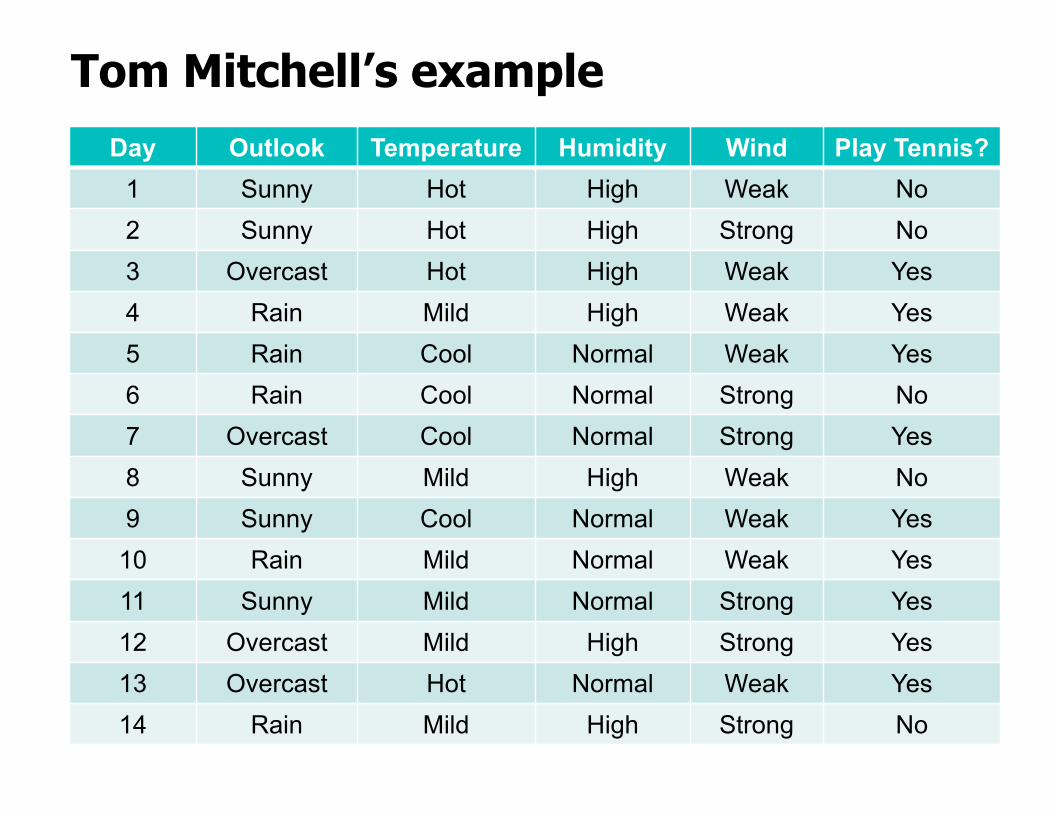
Tom Mitchell’s exampleDay Outlook Temperature Humidity Wind Play Tennis?
1 Sunny Hot High Weak No2 Sunny Hot High Strong No3 Overcast Hot High Weak Yes4 Rain Mild High Weak Yes5 Rain Cool Normal Weak Yes6 Rain Cool Normal Strong No7 Overcast Cool Normal Strong Yes8 Sunny Mild High Weak No9 Sunny Cool Normal Weak Yes
10 Rain Mild Normal Weak Yes11 Sunny Mild Normal Strong Yes12 Overcast Mild High Strong Yes13 Overcast Hot Normal Weak Yes14 Rain Mild High Strong No
Tree Induction
● Greedy strategy.– Split the records based on an attribute test
that optimizes certain criterion.
● Issues– Determine how to split the records
u How to specify the attribute test condition?u How to determine the best split?
– Determine when to stop splitting
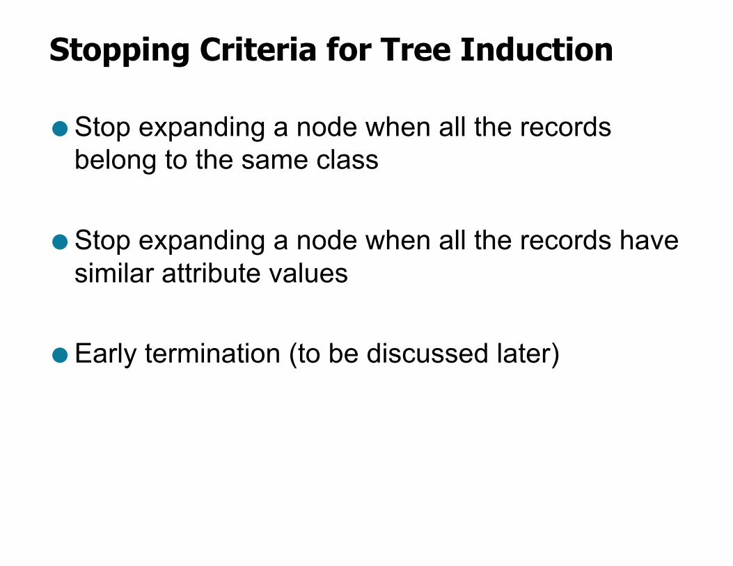
Stopping Criteria for Tree Induction
● Stop expanding a node when all the records belong to the same class
● Stop expanding a node when all the records have similar attribute values
● Early termination (to be discussed later)
Decision Tree Based Classification
● Advantages:– Inexpensive to construct– Extremely fast at classifying unknown records– Easy to interpret for small-sized trees– Accuracy is comparable to other classification
techniques for many simple data sets
Example: C4.5
● Simple depth-first construction.● Uses Information Gain● Sorts Continuous Attributes at each node.● Needs entire data to fit in memory.● Unsuitable for Large Datasets.
– Needs out-of-core sorting.
● You can download the software from:http://www.cse.unsw.edu.au/~quinlan/c4.5r8.tar.gz
– not there any longer, but you can Google it
Practical Issues of Classification
● Underfitting and Overfitting
● Missing Values
● Costs of Classification
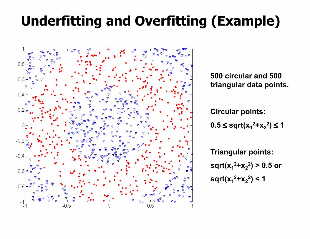
Underfitting and Overfitting (Example)
500 circular and 500 triangular data points.
Circular points:
0.5 £ sqrt(x12+x2
2) £ 1
Triangular points:
sqrt(x12+x2
2) > 0.5 or
sqrt(x12+x2
2) < 1
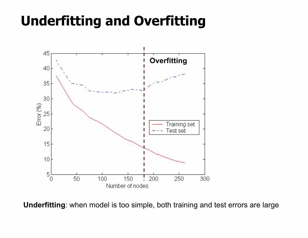
Underfitting and Overfitting
Overfitting
Underfitting: when model is too simple, both training and test errors are large
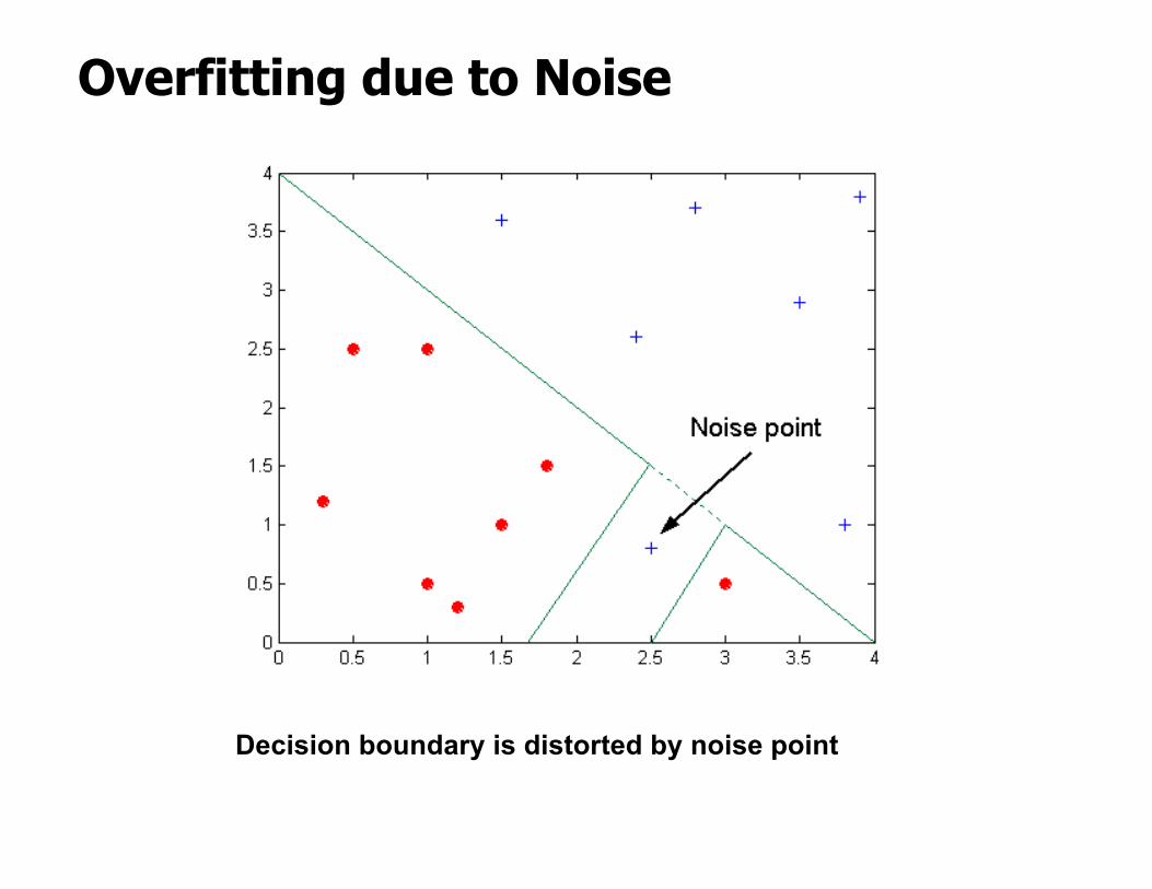
Overfitting due to Noise
Decision boundary is distorted by noise point
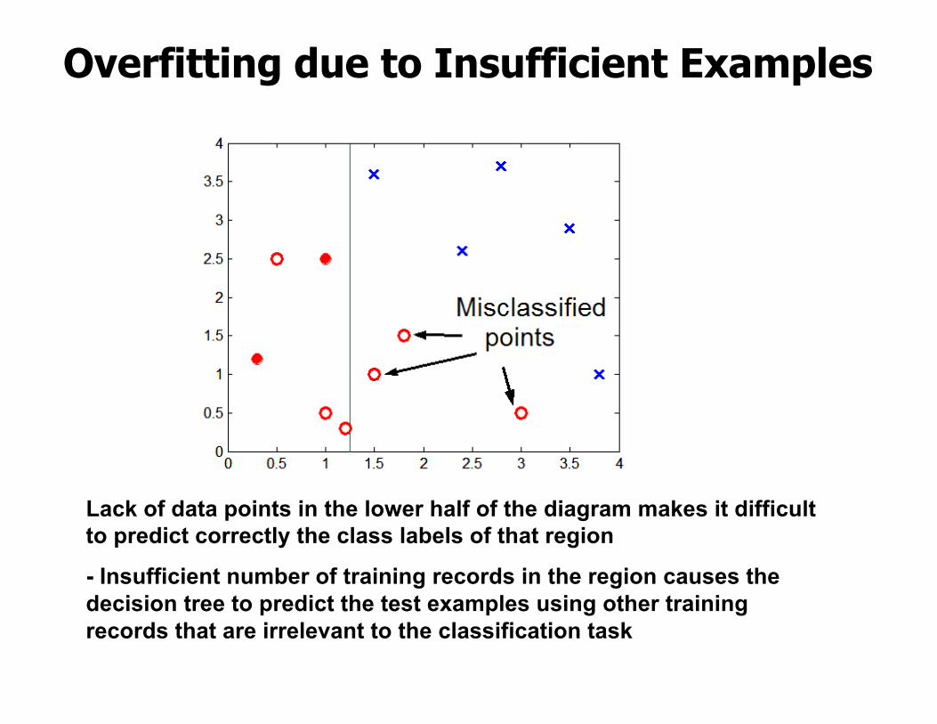
Overfitting due to Insufficient Examples
Lack of data points in the lower half of the diagram makes it difficult to predict correctly the class labels of that region
- Insufficient number of training records in the region causes the decision tree to predict the test examples using other training records that are irrelevant to the classification task
Notes on Overfitting
● Overfitting results in decision trees that are more complex than necessary
● Training error no longer provides a good estimate of how well the tree will perform on previously unseen records
● Need new ways for estimating errors
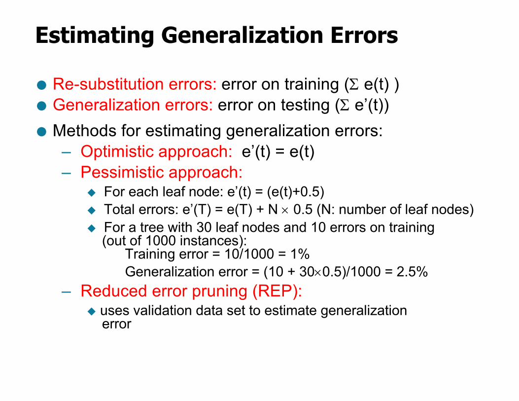
Estimating Generalization Errors
● Re-substitution errors: error on training (S e(t) )● Generalization errors: error on testing (S e’(t))● Methods for estimating generalization errors:
u For each leaf node: e’(t) = (e(t)+0.5) u Total errors: e’(T) = e(T) + N ´ 0.5 (N: number of leaf nodes)u For a tree with 30 leaf nodes and 10 errors on training
– Reduced error pruning (REP):u uses validation data set to estimate generalization
error
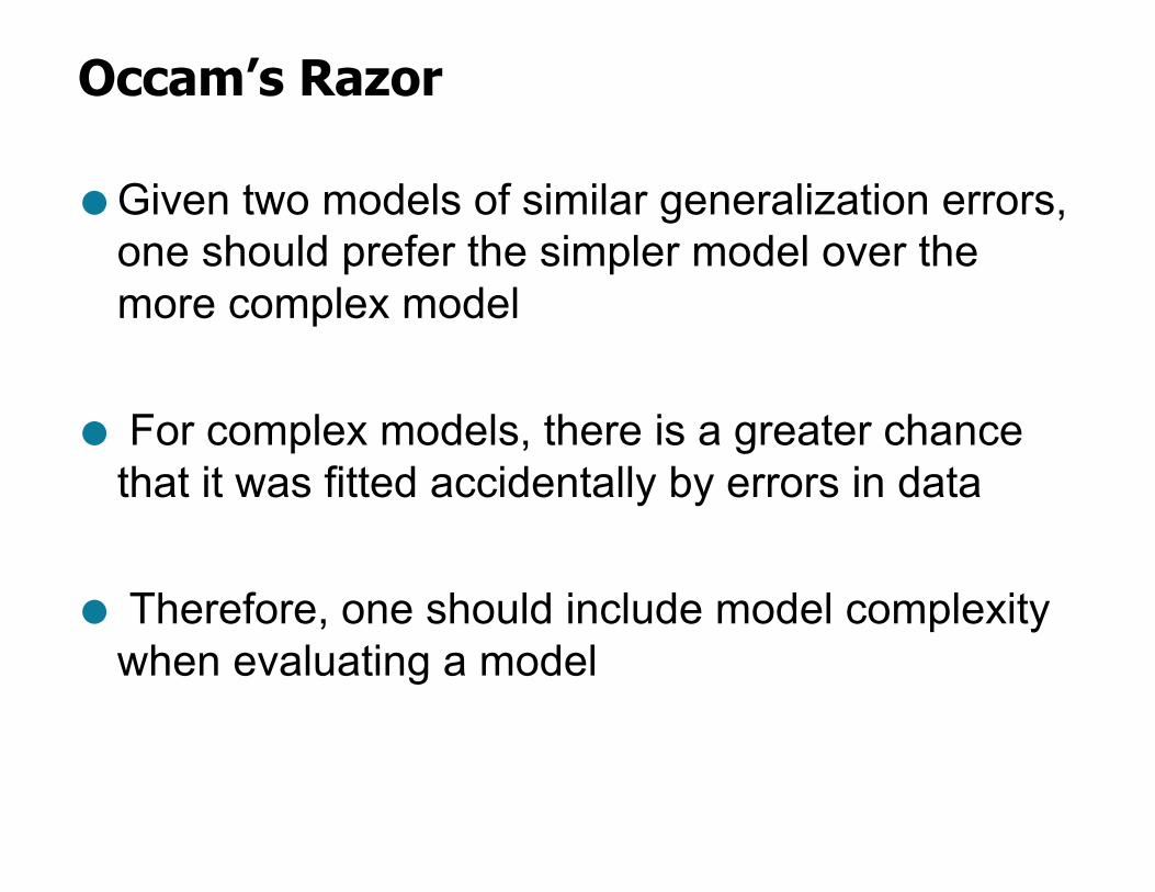
Occam’s Razor
● Given two models of similar generalization errors, one should prefer the simpler model over the more complex model
● For complex models, there is a greater chance that it was fitted accidentally by errors in data
● Therefore, one should include model complexity when evaluating a model
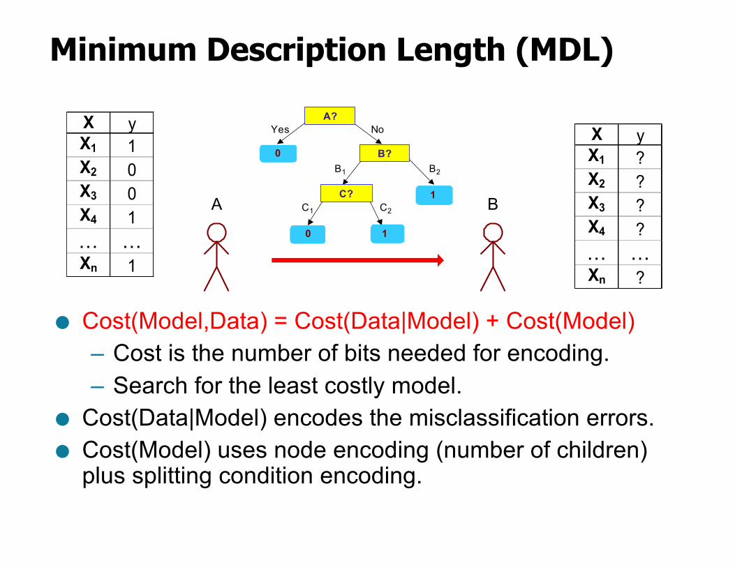
Minimum Description Length (MDL)
● Cost(Model,Data) = Cost(Data|Model) + Cost(Model)– Cost is the number of bits needed for encoding.– Search for the least costly model.
● Cost(Data|Model) encodes the misclassification errors.● Cost(Model) uses node encoding (number of children)
plus splitting condition encoding.
A B
A?
B?
C?
10
0
1
Yes No
B1 B2
C1 C2
X yX1 1X2 0X3 0X4 1… …Xn 1
X yX1 ?X2 ?X3 ?X4 ?… …Xn ?
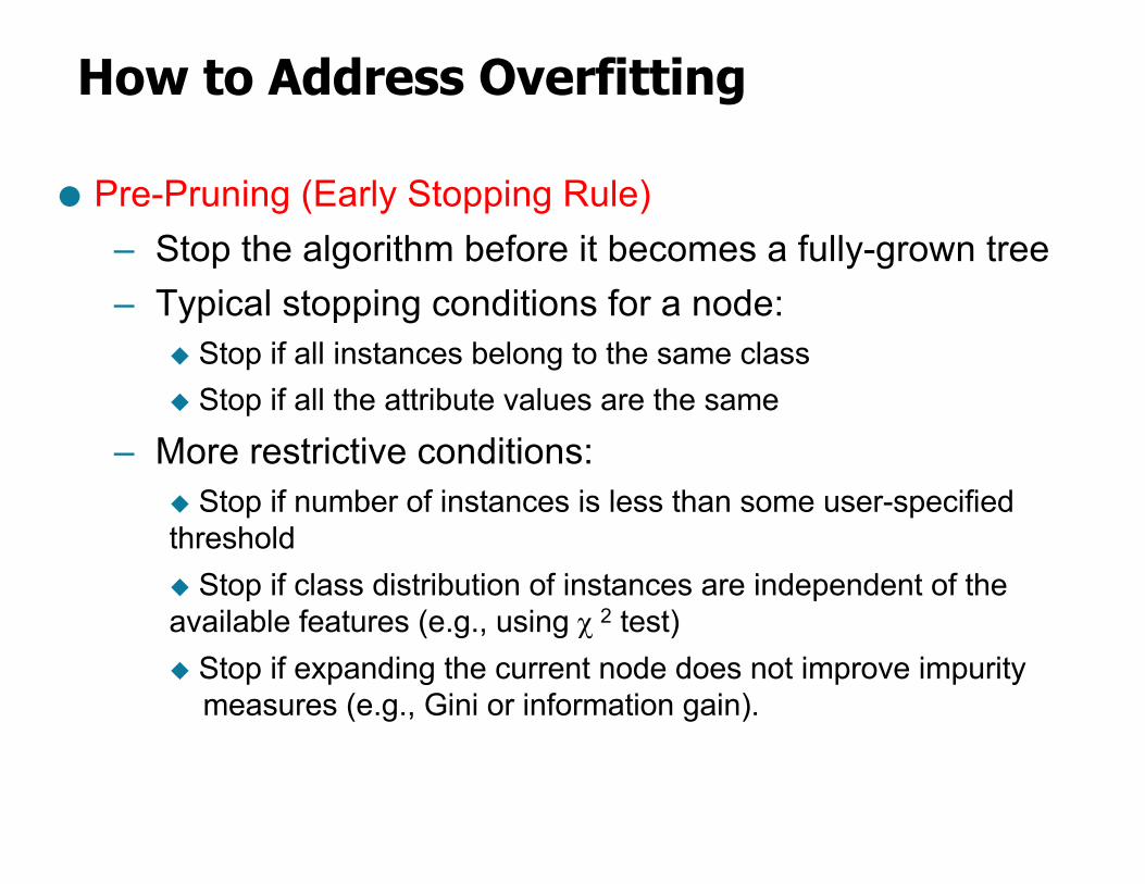
How to Address Overfitting
● Pre-Pruning (Early Stopping Rule)– Stop the algorithm before it becomes a fully-grown tree– Typical stopping conditions for a node:
u Stop if all instances belong to the same classu Stop if all the attribute values are the same
– More restrictive conditions:u Stop if number of instances is less than some user-specified thresholdu Stop if class distribution of instances are independent of the available features (e.g., using c 2 test)u Stop if expanding the current node does not improve impurity
measures (e.g., Gini or information gain).
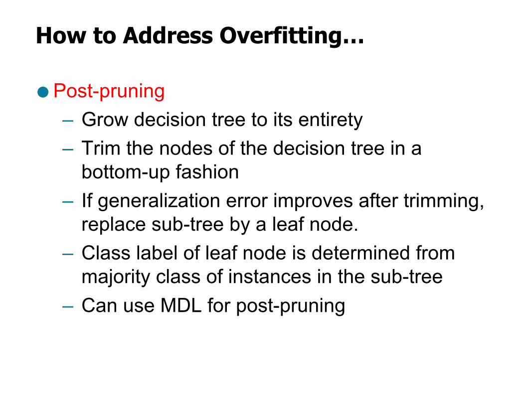
How to Address Overfitting…
● Post-pruning– Grow decision tree to its entirety– Trim the nodes of the decision tree in a
bottom-up fashion– If generalization error improves after trimming,
replace sub-tree by a leaf node.– Class label of leaf node is determined from
majority class of instances in the sub-tree– Can use MDL for post-pruning
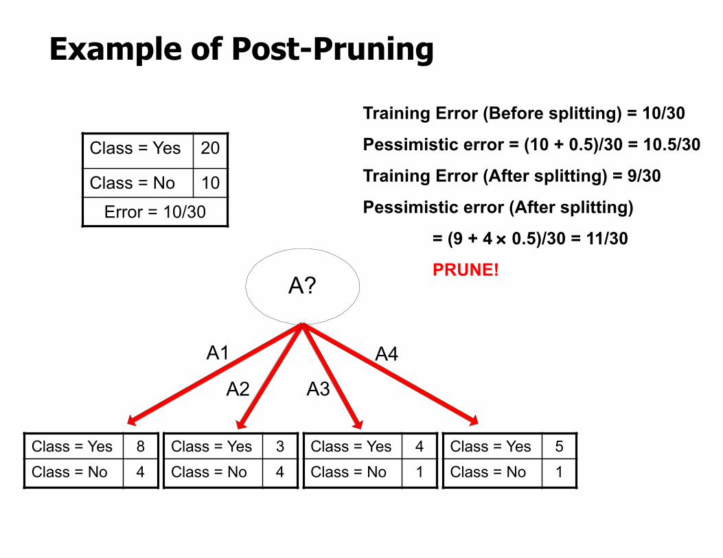
Example of Post-Pruning
A?
A1
A2 A3
A4
Class = Yes 20
Class = No 10Error = 10/30
Training Error (Before splitting) = 10/30
Pessimistic error = (10 + 0.5)/30 = 10.5/30
Training Error (After splitting) = 9/30
Pessimistic error (After splitting)
= (9 + 4 ´ 0.5)/30 = 11/30
PRUNE!
Class = Yes 8Class = No 4
Class = Yes 3Class = No 4
Class = Yes 4Class = No 1
Class = Yes 5Class = No 1
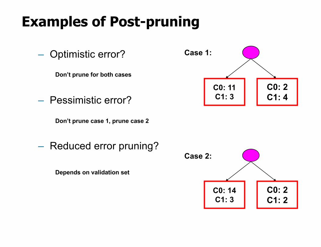
Examples of Post-pruning
– Optimistic error?
– Pessimistic error?
– Reduced error pruning?
C0: 11C1: 3
C0: 2C1: 4
C0: 14C1: 3
C0: 2C1: 2
Don’t prune for both cases
Don’t prune case 1, prune case 2
Case 1:
Case 2:
Depends on validation set
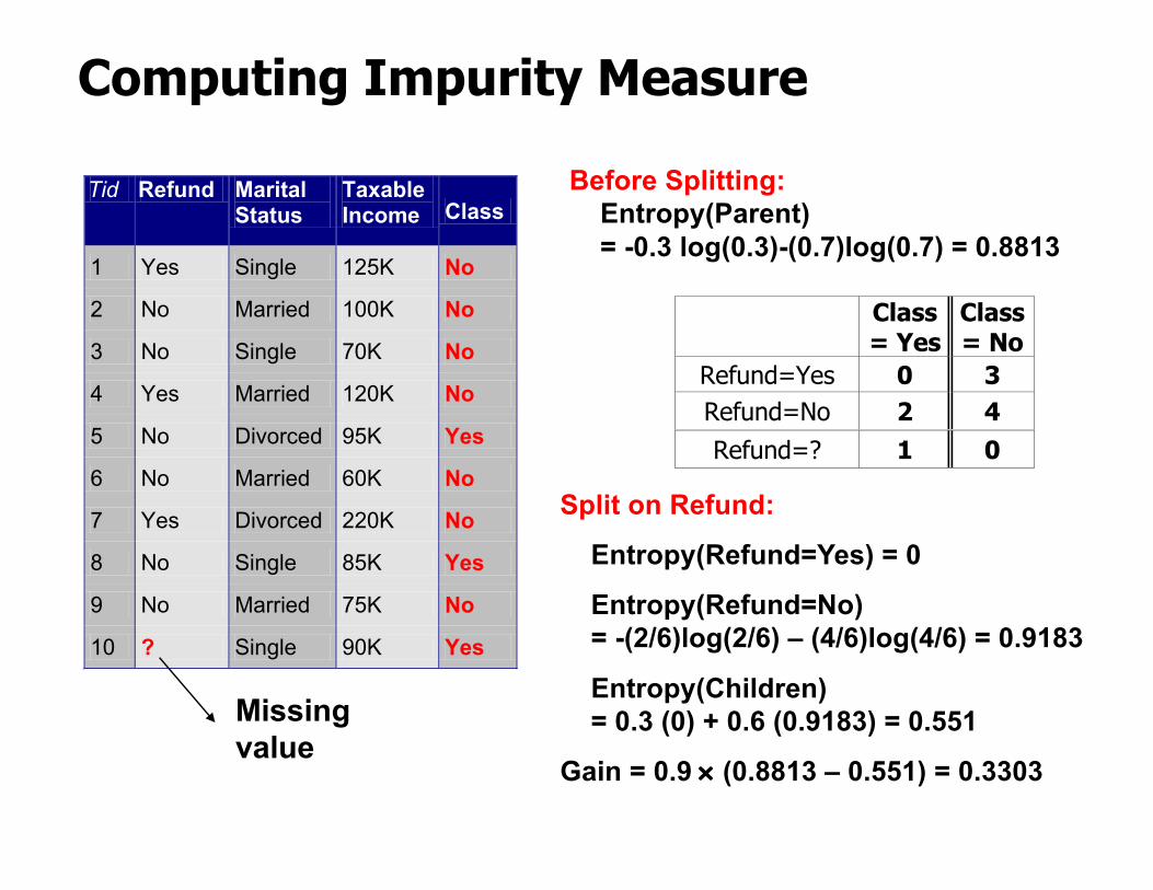
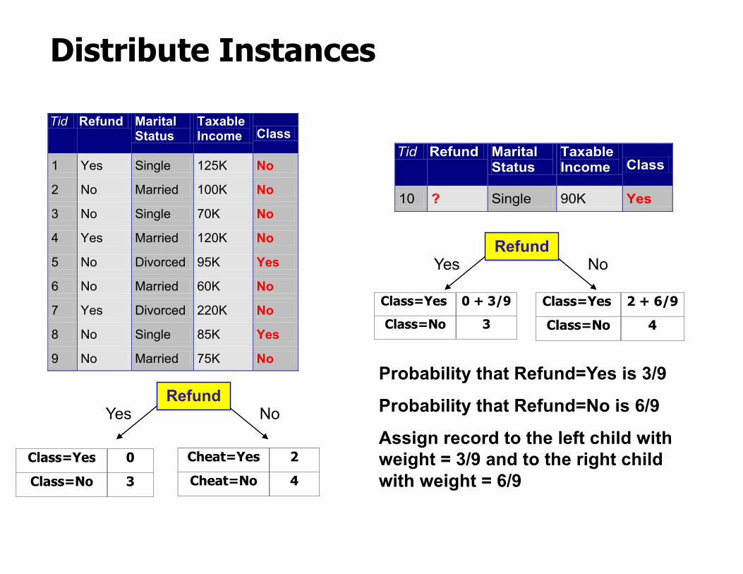
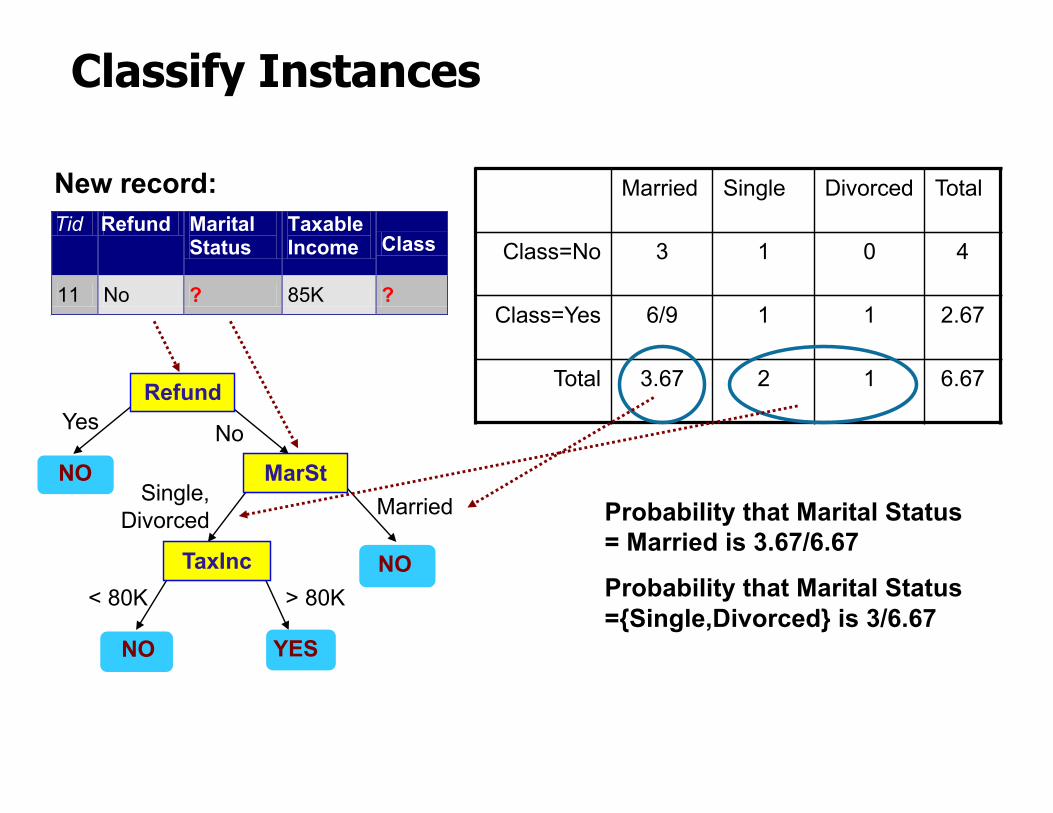
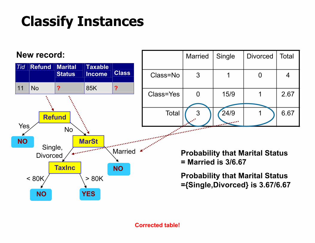
Handling Missing Attribute Values
● Missing values affect decision tree construction in three different ways:– Affects how impurity measures are computed– Affects how to distribute instance with missing
value to child nodes– Affects how a test instance with missing value
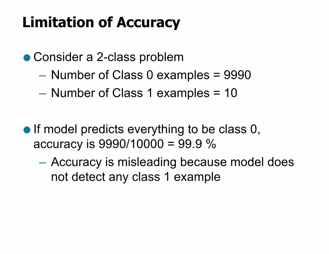
● Consider a 2-class problem– Number of Class 0 examples = 9990– Number of Class 1 examples = 10
● If model predicts everything to be class 0, accuracy is 9990/10000 = 99.9 %– Accuracy is misleading because model does
not detect any class 1 example
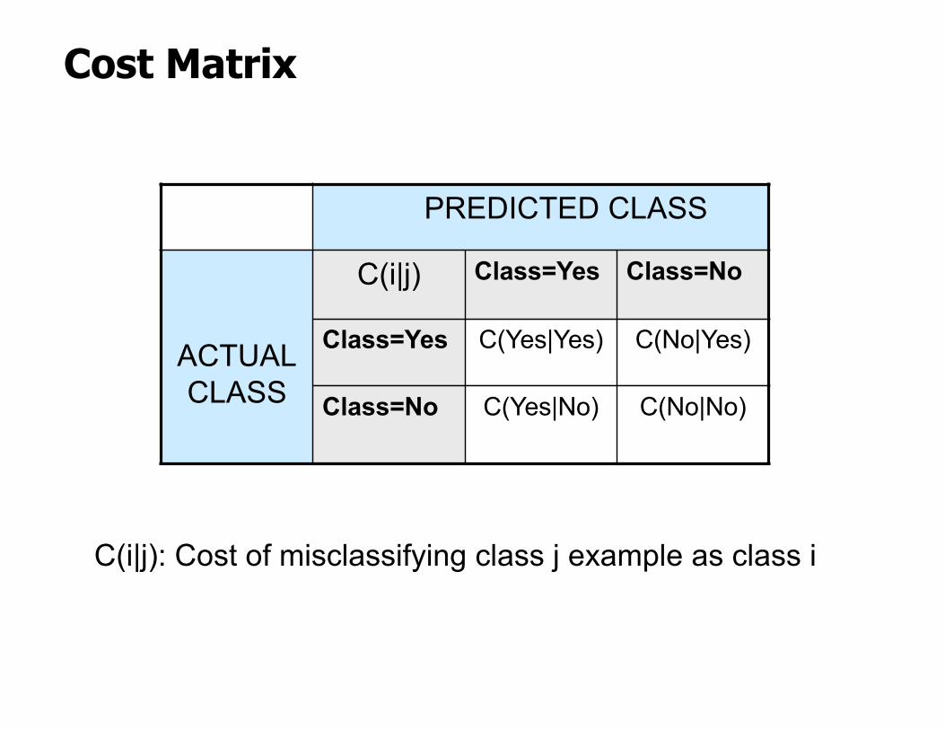
Cost Matrix
PREDICTED CLASS
ACTUALCLASS
C(i|j) Class=Yes Class=No
Class=Yes C(Yes|Yes) C(No|Yes)
Class=No C(Yes|No) C(No|No)
C(i|j): Cost of misclassifying class j example as class i
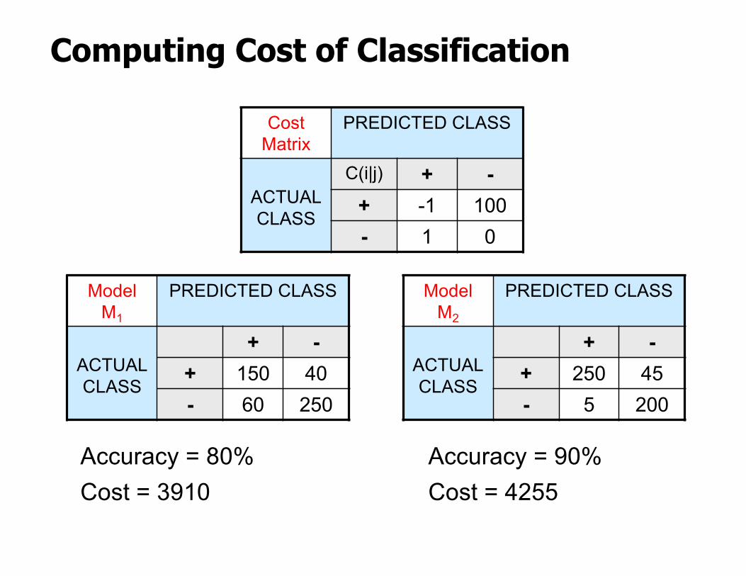
Computing Cost of Classification
Cost Matrix
PREDICTED CLASS
ACTUALCLASS
C(i|j) + -+ -1 100- 1 0
Model M1
PREDICTED CLASS
ACTUALCLASS
+ -+ 150 40- 60 250
Model M2
PREDICTED CLASS
ACTUALCLASS
+ -+ 250 45- 5 200
Accuracy = 80%Cost = 3910
Accuracy = 90%Cost = 4255
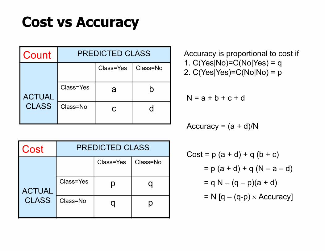
Cost vs Accuracy
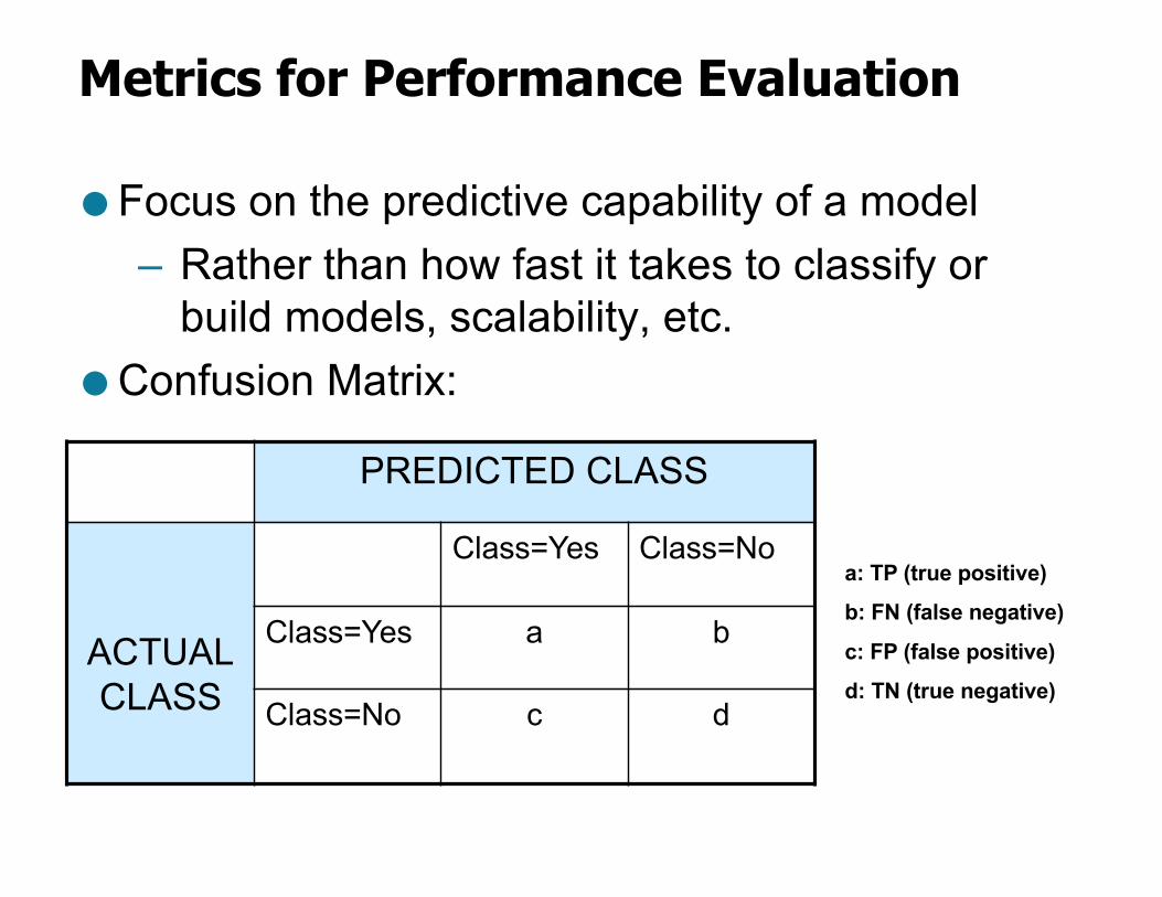
Count PREDICTED CLASS
ACTUALCLASS
Class=Yes Class=No
Class=Yes a b
Class=No c d
Cost PREDICTED CLASS
ACTUALCLASS
Class=Yes Class=No
Class=Yes p q
Class=No q p
N = a + b + c + d
Accuracy = (a + d)/N
Cost = p (a + d) + q (b + c)
= p (a + d) + q (N – a – d)
= q N – (q – p)(a + d)
= N [q – (q-p) ´ Accuracy]
Accuracy is proportional to cost if1. C(Yes|No)=C(No|Yes) = q 2. C(Yes|Yes)=C(No|No) = p
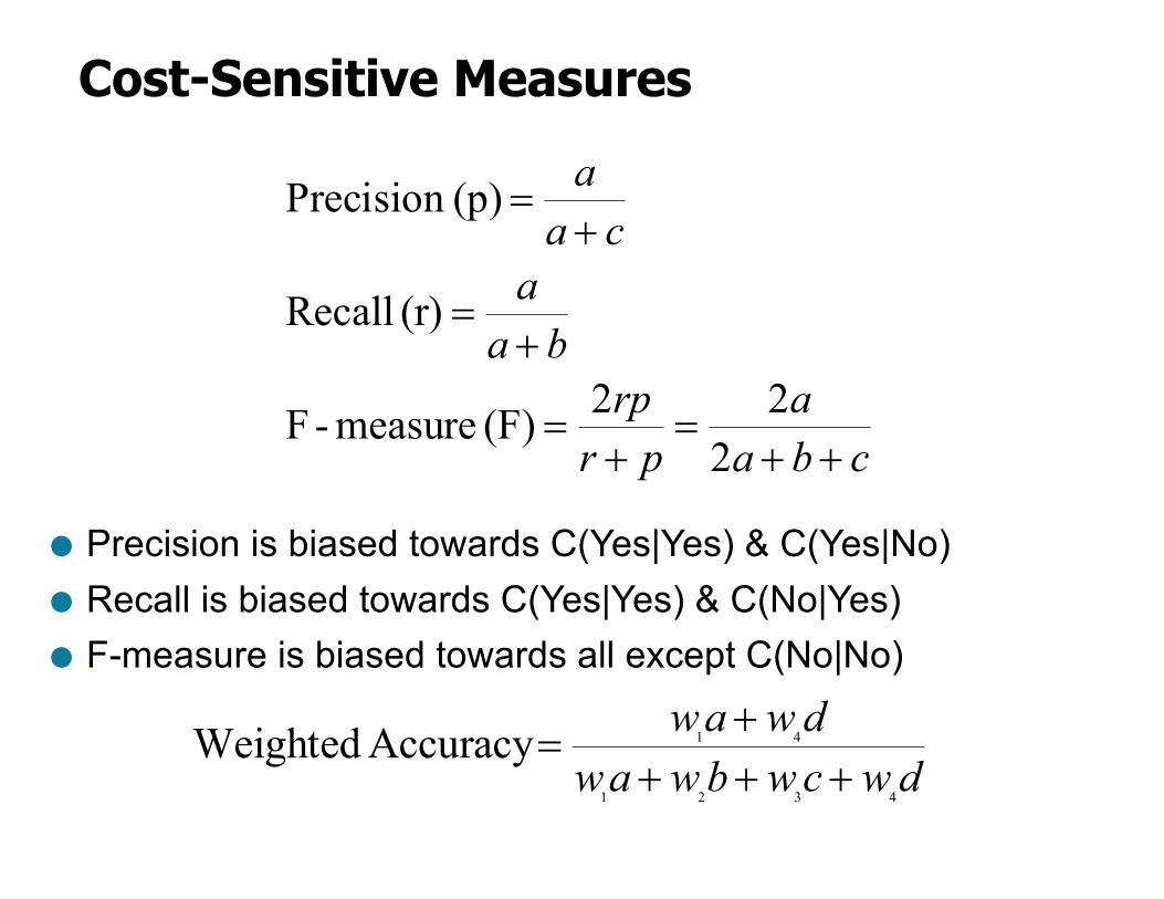
Cost-Sensitive Measures
cbaa
prrp
baa
caa
++=
+=
+=
+=
222(F) measure-F
(r) Recall
(p)Precision
● Precision is biased towards C(Yes|Yes) & C(Yes|No)● Recall is biased towards C(Yes|Yes) & C(No|Yes)● F-measure is biased towards all except C(No|No)
dwcwbwawdwaw
4321
41Accuracy Weighted+++
+=
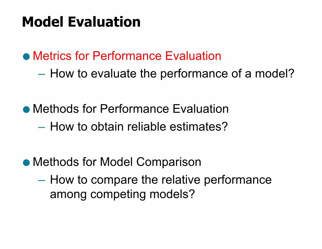
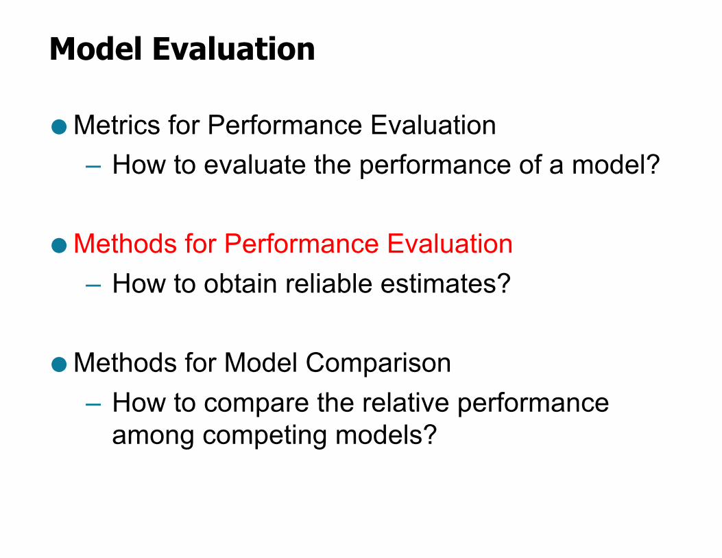
Model Evaluation
● Metrics for Performance Evaluation– How to evaluate the performance of a model?
● Methods for Performance Evaluation– How to obtain reliable estimates?
● Methods for Model Comparison– How to compare the relative performance
among competing models?
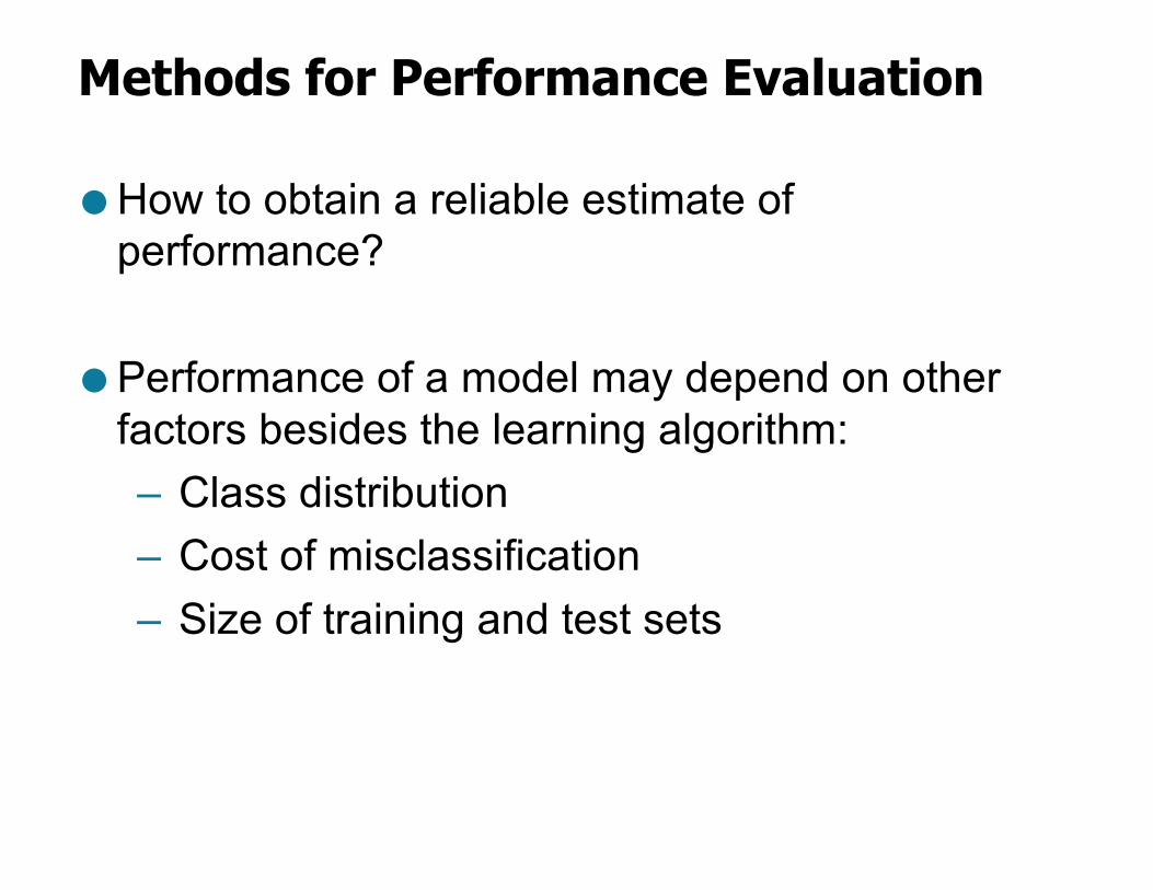
Methods for Performance Evaluation
● How to obtain a reliable estimate of performance?
● Performance of a model may depend on other factors besides the learning algorithm:– Class distribution– Cost of misclassification– Size of training and test sets
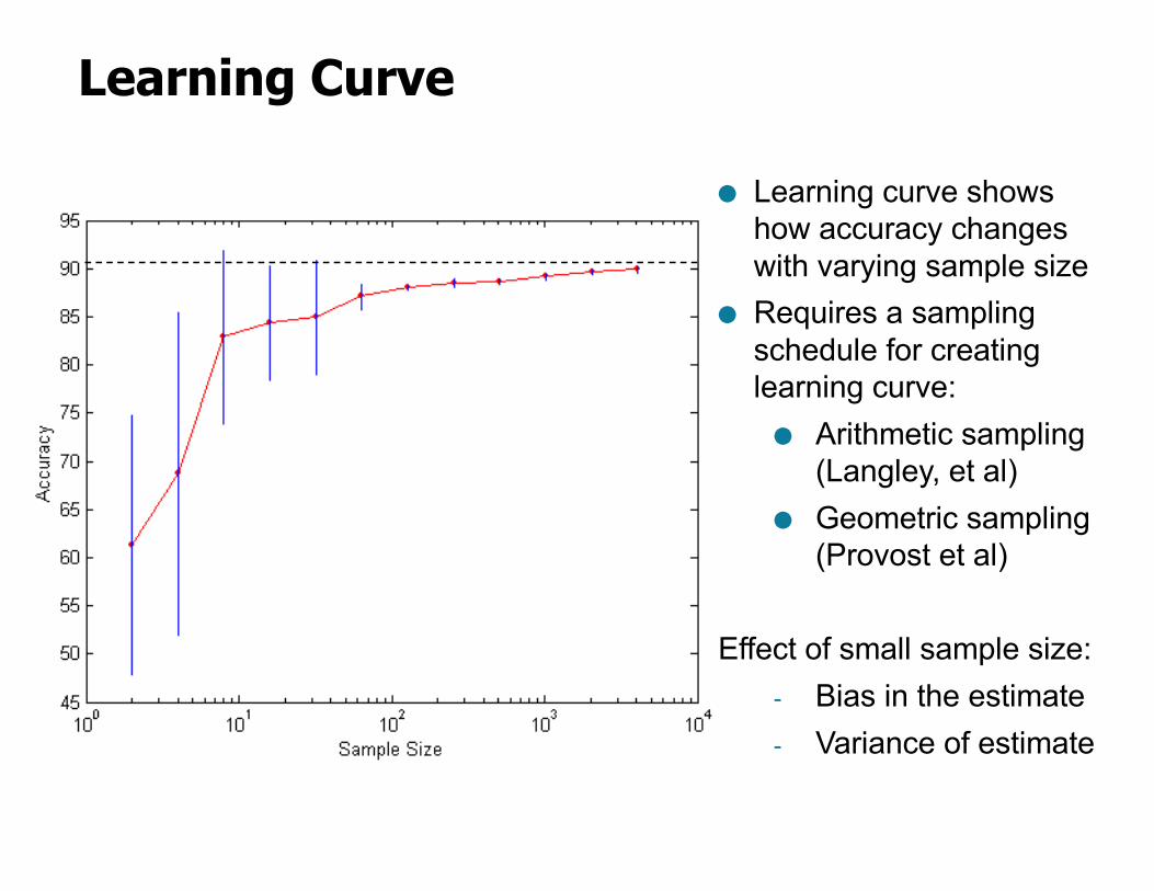
Learning Curve
● Learning curve shows how accuracy changes with varying sample size
● Requires a sampling schedule for creating learning curve:● Arithmetic sampling
(Langley, et al)● Geometric sampling
(Provost et al)
Effect of small sample size:- Bias in the estimate- Variance of estimate
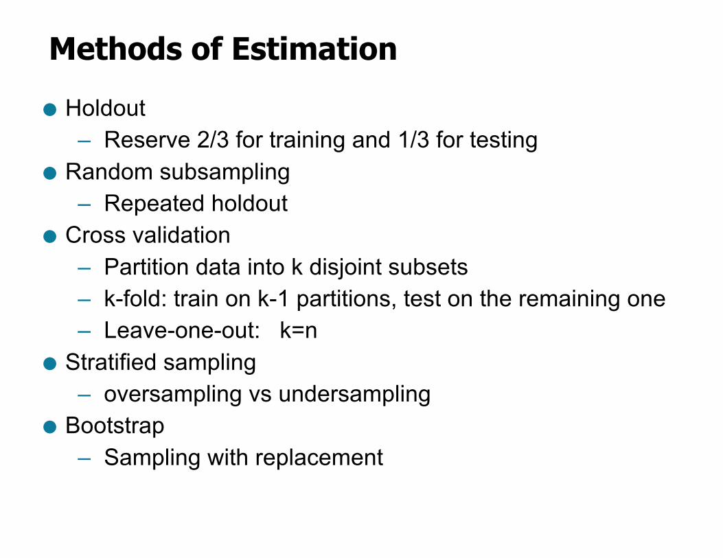
Methods of Estimation● Holdout
– Reserve 2/3 for training and 1/3 for testing ● Random subsampling
– Repeated holdout● Cross validation
– Partition data into k disjoint subsets– k-fold: train on k-1 partitions, test on the remaining one– Leave-one-out: k=n
● Stratified sampling – oversampling vs undersampling
● Bootstrap– Sampling with replacement
Model Evaluation
● Metrics for Performance Evaluation– How to evaluate the performance of a model?
● Methods for Performance Evaluation– How to obtain reliable estimates?
● Methods for Model Comparison– How to compare the relative performance
among competing models?
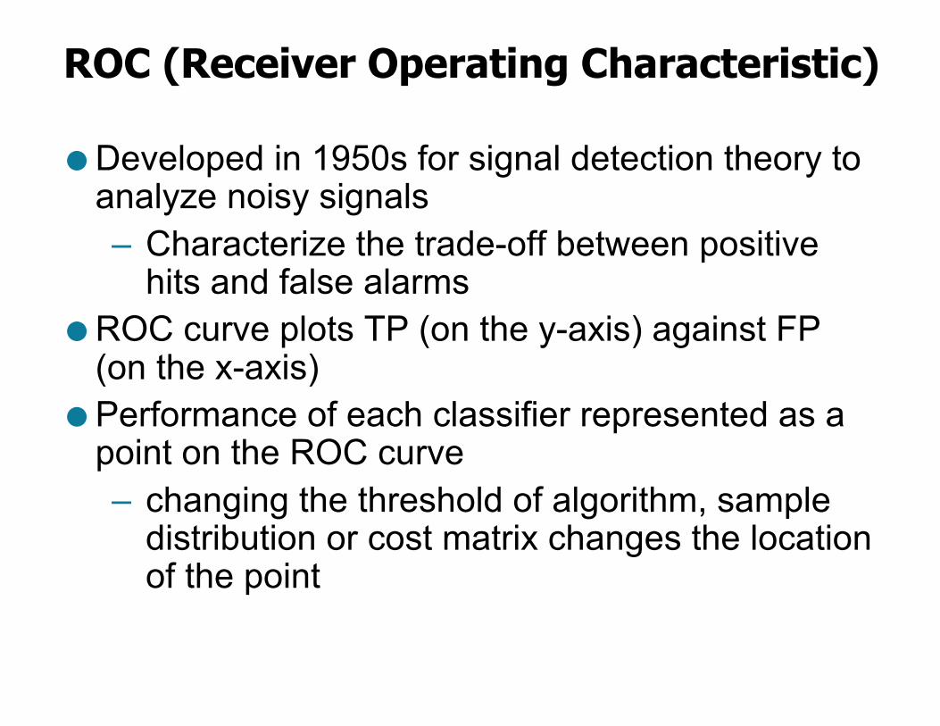
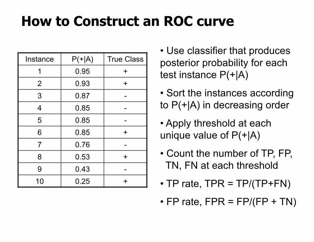
ROC (Receiver Operating Characteristic)
● Developed in 1950s for signal detection theory to analyze noisy signals – Characterize the trade-off between positive
hits and false alarms● ROC curve plots TP (on the y-axis) against FP
(on the x-axis)● Performance of each classifier represented as a
point on the ROC curve– changing the threshold of algorithm, sample
distribution or cost matrix changes the location of the point
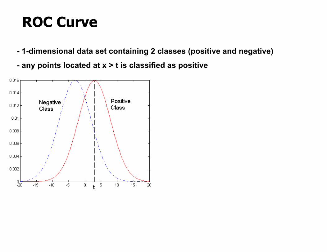
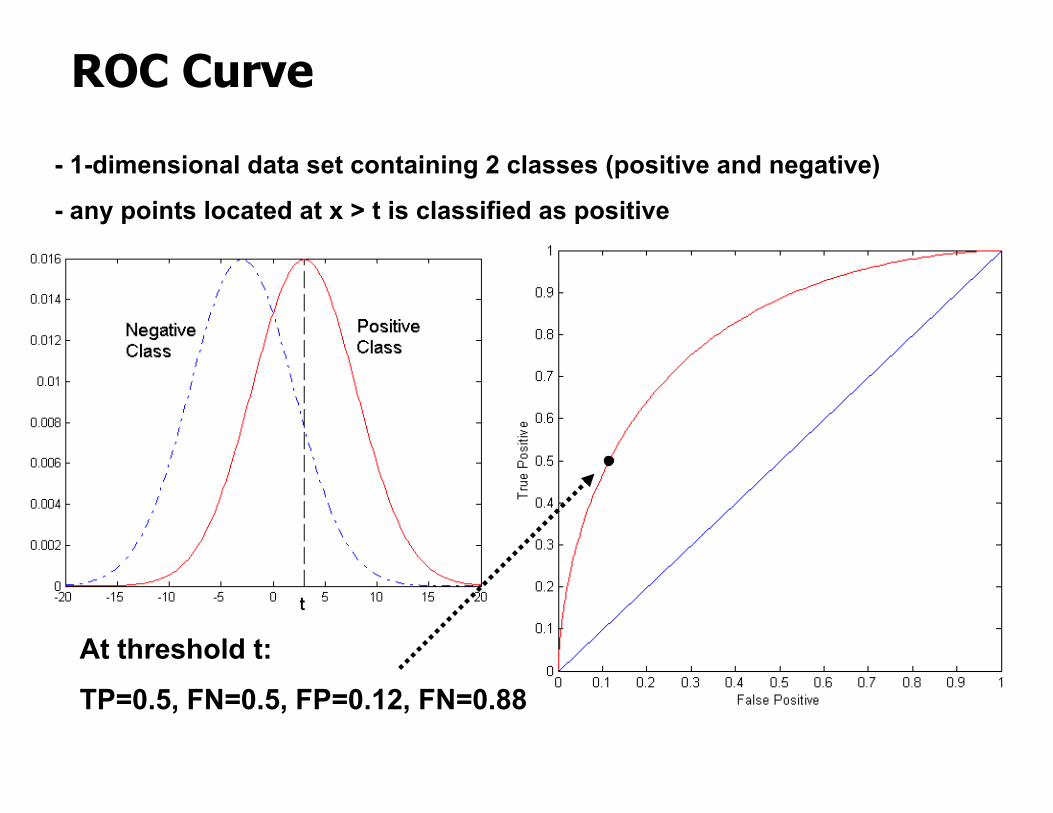
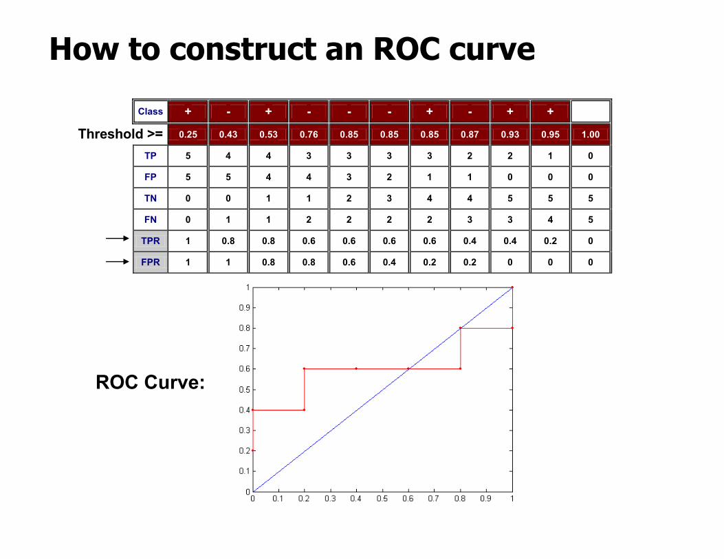
ROC Curve
- 1-dimensional data set containing 2 classes (positive and negative)
- any points located at x > t is classified as positive
At threshold t:TP=0.5, FN=0.5, FP=0.12, FN=0.88
ROC Curve
- 1-dimensional data set containing 2 classes (positive and negative)
- any points located at x > t is classified as positive
ROC Curve
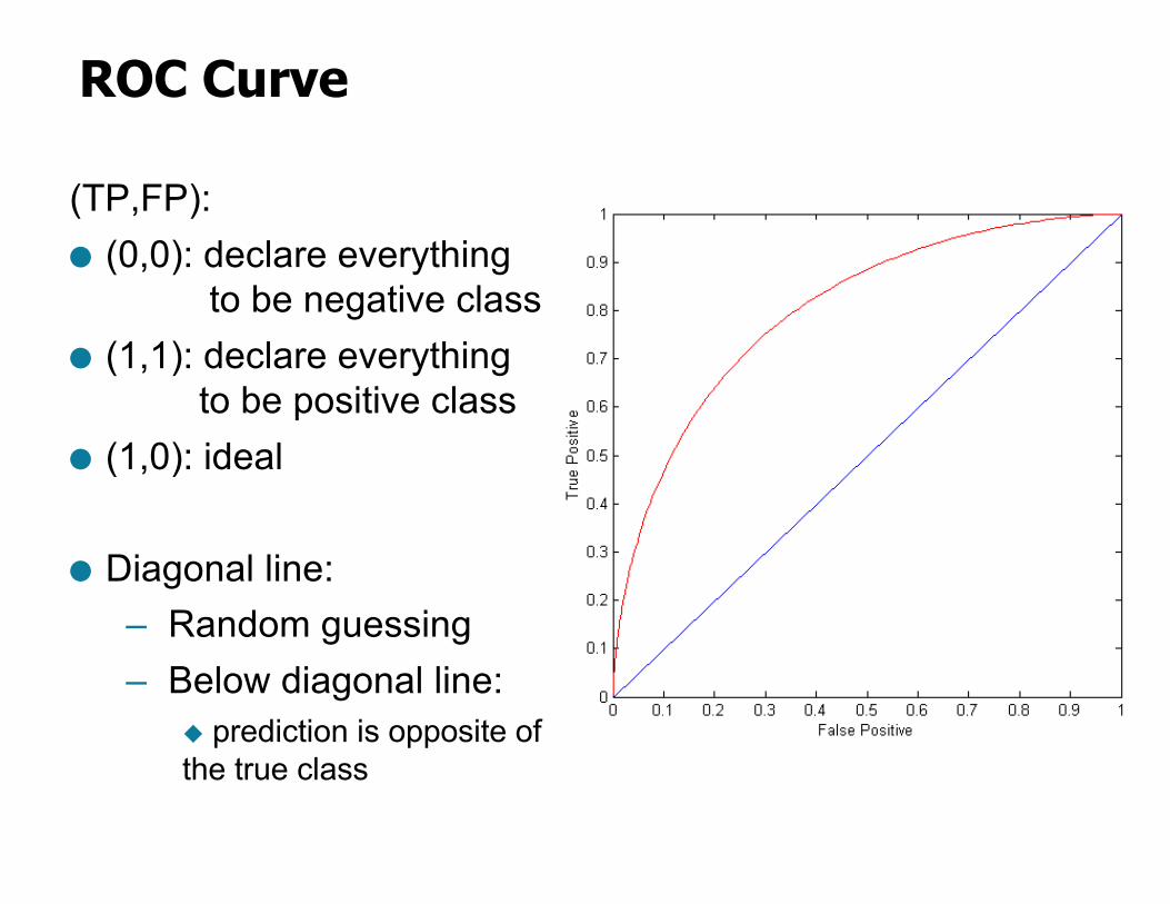
(TP,FP):● (0,0): declare everything
to be negative class● (1,1): declare everything
to be positive class● (1,0): ideal
● Diagonal line:– Random guessing– Below diagonal line:
u prediction is opposite of the true class
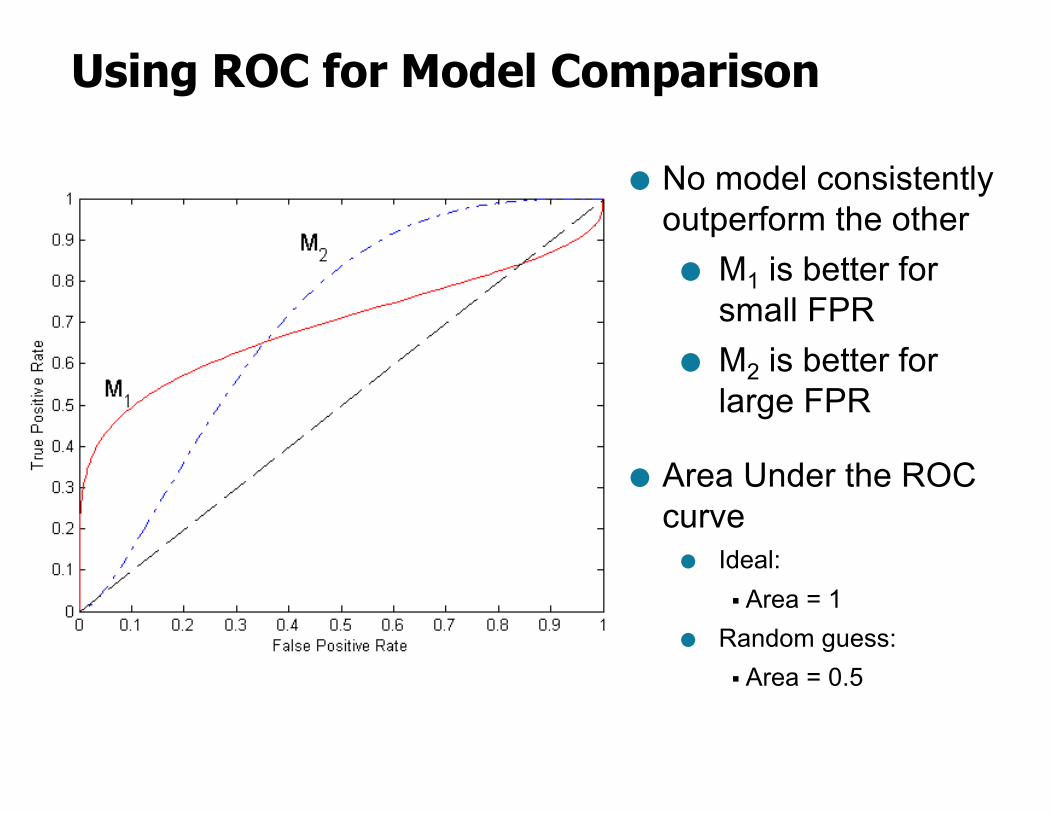
Using ROC for Model Comparison
● No model consistently outperform the other● M1 is better for