Data Mining: Concepts and Techniques -...

November 26, 2006 Data Mining: Concepts and Techniques 1

Data Mining: Concepts and Techniques

— Slides for Textbook —— Chapter 5 —


Chapter 5: Concept Description: Characterization and Comparison

What is concept description?

Data generalization and summarization-based characterization

Analytical characterization: Analysis of attribute relevance

Mining class comparisons: Discriminating between different classes

Mining descriptive statistical measures in large databases

Discussion

Summary

What is Concept Description?

Descriptive vs. predictive data miningDescriptive mining: describes concepts or task-relevant data sets in concise, summarative, informative, discriminative formsPredictive mining: Based on data and analysis, constructs models for the database, and predicts the trend and properties of unknown data

Concept description: Characterization: provides a concise and succinct summarization of the given collection of dataComparison: provides descriptions comparing two or more collections of data


Concept Description vs. OLAP

Concept description: can handle complex data types of the

attributes and their aggregationsa more automated process

OLAP: restricted to a small number of dimension and measure typesuser-controlled process



What is concept description? Data generalization and summarization-based characterizationAnalytical characterization: Analysis of attribute relevanceMining class comparisons: Discriminating between different classesMining descriptive statistical measures in large databasesDiscussionSummary


Data Generalization and Summarization-based Characterization

Data generalization

A process which abstracts a large set of task-relevant data in a database from a low conceptual levels to higher ones.

Approaches:

Data cube approach(OLAP approach)

Attribute-oriented induction approach

1

2

3

4

5Conceptual levels


Characterization: Data Cube Approach

Data are stored in data cubeIdentify expensive computations

e.g., count( ), sum( ), average( ), max( )Perform computations and store results in data cubesGeneralization and specialization can be performed on a data cube by roll-up and drill-downAn efficient implementation of data generalization


Data Cube Approach (Cont…)

Limitationscan only handle data types of dimensions tosimple nonnumeric data and of measures tosimple aggregated numeric values.

Lack of intelligent analysis, can’t tell which dimensions should be used and what levels should the generalization reach


Attribute-Oriented Induction

Proposed in 1989 (KDD ‘89 workshop)

Not confined to categorical data nor particular measures.

How it is done?

Collect the task-relevant data (initial relation) using a relational database query

Perform generalization by attribute removal or attribute generalization.

Apply aggregation by merging identical, generalized tuples and accumulating their respective counts

Interactive presentation with users

Basic Principles of Attribute-Oriented Induction

Data focusing: task-relevant data, including dimensions, and the result is the initial relation.

Attribute-removal: remove attribute A if there is a large set of distinct values for A but (1) there is no generalization operator on A, or (2) A’s higher level concepts are expressed in terms of other attributes.

Attribute-generalization: If there is a large set of distinct values for A, and there exists a set of generalization operators on A, then select an operator and generalize A.

Attribute-threshold control: typical 2-8, specified/default.

Generalized relation threshold control: control the final relation/rule size. see example

Attribute-Oriented Induction: Basic Algorithm

InitialRel: Query processing of task-relevant data, deriving the initial relation.

PreGen: Based on the analysis of the number of distinct values in each attribute, determine generalization plan for each attribute: removal? or how high to generalize?

PrimeGen: Based on the PreGen plan, perform generalization to the right level to derive a “prime generalized relation”, accumulating the counts.

Presentation: User interaction: (1) adjust levels by drilling, (2) pivoting, (3) mapping into rules, cross tabs, visualization presentations.


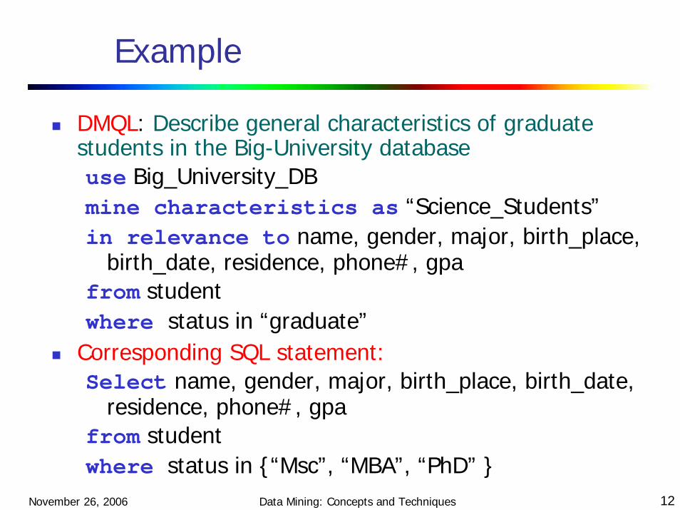
Example

DMQL: Describe general characteristics of graduate students in the Big-University databaseuse Big_University_DBmine characteristics as “Science_Students”in relevance to name, gender, major, birth_place,

birth_date, residence, phone#, gpafrom studentwhere status in “graduate”

Corresponding SQL statement:Select name, gender, major, birth_place, birth_date,

residence, phone#, gpafrom studentwhere status in {“Msc”, “MBA”, “PhD” }

Class Characterization: An Example

Name Gender Major Birth-Place Birth_date Residence Phone # GPA

JimWoodman

M CS Vancouver,BC,Canada

8-12-76 3511 Main St.,Richmond

687-4598 3.67

ScottLachance

M CS Montreal, Que,Canada

28-7-75 345 1st Ave.,Richmond

253-9106 3.70

Laura Lee…

F…

Physics…

Seattle, WA, USA…

25-8-70…

125 Austin Ave.,Burnaby…

420-5232…

3.83…

Removed Retained Sci,Eng,Bus

Country Age range City Removed Excl,VG,..

Gender Major Birth_region Age_range Residence GPA Count M Science Canada 20-25 Richmond Very-good 16 F Science Foreign 25-30 Burnaby Excellent 22 … … … … … … …

Birth_Region

GenderCanada Foreign Total

M 16 14 30 F 10 22 32

Total 26 36 62

Prime Generalized Relation

Initial Relation

Presentation of Generalized Results

Generalized relation:

Relations where some or all attributes are generalized, with counts or other aggregation values accumulated.

Cross tabulation:

Mapping results into cross tabulation form (similar to contingency tables).

Visualization techniques:

Pie charts, bar charts, curves, cubes, and other visual forms.

Quantitative characteristic rules:

Mapping generalized result into characteristic rules with quantitative information associated with it, e.g.,

.%]47:["")(_%]53:["")(_)()(

tforeignxregionbirthtCanadaxregionbirthxmalexgrad

=∨=⇒∧


Presentation—Generalized Relation


Presentation—Crosstab


Implementation by Cube Technology

Construct a data cube on-the-fly for the given data mining query

Facilitate efficient drill-down analysisMay increase the response timeA balanced solution: precomputation of “subprime”relation

Use a predefined & precomputed data cubeConstruct a data cube beforehandFacilitate not only the attribute-oriented induction, but also attribute relevance analysis, dicing, slicing, roll-up and drill-downCost of cube computation and the nontrivial storage overhead








Discussion

Summary


Characterization vs. OLAP

Similarity:

Presentation of data summarization at multiple levels of abstraction.

Interactive drilling, pivoting, slicing and dicing.

Differences:

Automated desired level allocation.

Dimension relevance analysis and ranking when there are many relevant dimensions.

Sophisticated typing on dimensions and measures.

Analytical characterization: data dispersion analysis.


Attribute Relevance Analysis

Why?Which dimensions should be included? How high level of generalization?Automatic VS. InteractiveReduce # attributes; Easy to understand patterns

What?statistical method for preprocessing data

filter out irrelevant or weakly relevant attributes retain or rank the relevant attributes

relevance related to dimensions and levelsanalytical characterization, analytical comparison


Attribute relevance analysis (cont’d)

How?Data CollectionAnalytical Generalization

Use information gain analysis (e.g., entropy or other measures) to identify highly relevant dimensions and levels.

Relevance AnalysisSort and select the most relevant dimensions and levels.

Attribute-oriented Induction for class descriptionOn selected dimension/level

OLAP operations (e.g. drilling, slicing) on relevance rules


Relevance Measures

Quantitative relevance measure determines the classifying power of an attribute within a set of data.Methods

information gain (ID3)gain ratio (C4.5)gini indexχ2 contingency table statisticsuncertainty coefficient


Information-Theoretic Approach

Decision treeeach internal node tests an attributeeach branch corresponds to attribute valueeach leaf node assigns a classification

ID3 algorithmbuild decision tree based on training objects with known class labels to classify testing objectsrank attributes with information gain measureminimal height

the least number of tests to classify an object


Top-Down Induction of Decision Tree

Attributes = {Outlook, Temperature, Humidity, Wind}

Outlook

Humidity Wind

sunny rainovercast

yes

no yes

high normal

no

strong weak

yes

PlayTennis = {yes, no}


Entropy and Information Gain

S contains si tuples of class Ci for i = {1, …, m} Information measures info required to classify any arbitrary tuple

Entropy of attribute A with values {a1,a2,…,av}

Information gained by branching on attribute A

sslog

ss),...,s,ssI( i

m

i

im21 2

1∑=

−=

)s,...,s(Is

s...sE(A) mjj

v

j

mjj1

1

1∑=

++=

E(A))s,...,s,I(sGain(A) m −= 21


Example

For attribute sex

M

F

C1

C2

1/2

1/2

Gain = 1

M=1/2F=1/2

M=1/2F=1/2

C1

C2

1/2

1/2

M

F

C1

C2

1/4

3/4

Gain = 0

Gain less than but near 1

C1

C2

1/4

3/4

Gain greater than but near 1

M=1/2F=1/2

M=1/2F=1/2



Example: Analytical Characterization

TaskMine general characteristics describing graduate students using analytical characterization

Givenattributes name, gender, major, birth_place, birth_date, phone#, and gpaGen(ai) = concept hierarchies on ai

Ui = attribute analytical thresholds for ai

Ti = attribute generalization thresholds for ai

R = attribute relevance threshold


Example: Analytical Characterization (cont’d)

1. Data collectiontarget class: graduate studentcontrasting class: undergraduate student

2. Analytical generalization using Ui

attribute removalremove name and phone#

attribute generalizationgeneralize major, birth_place, birth_date and gpaaccumulate counts

candidate relation: gender, major, birth_country, age_range and gpa


Example: Analytical characterization (2)

gender major birth_country age_range gpa count

M Science Canada 20-25 Very_good 16F Science Foreign 25-30 Excellent 22M Engineering Foreign 25-30 Excellent 18F Science Foreign 25-30 Excellent 25M Science Canada 20-25 Excellent 21F Engineering Canada 20-25 Excellent 18

Candidate relation for Target class: Graduate students (Σ=120)

gender major birth_country age_range gpa count

M Science Foreign <20 Very_good 18F Business Canada <20 Fair 20M Business Canada <20 Fair 22F Science Canada 20-25 Fair 24M Engineering Foreign 20-25 Very_good 22F Engineering Canada <20 Excellent 24

Candidate relation for Contrasting class: Undergraduate students (Σ=130)



3. Relevance analysisCalculate expected info required to classify an arbitrary tuple

Calculate entropy of each attribute: e.g. major

99880250130

250130

250120

250120130120 2221 .loglog),I()s,I(s =−−==

For major=”Science”: S11=84 S21=42 I(s11,s21)=0.9183

For major=”Engineering”: S12=36 S22=46 I(s12,s22)=0.9892

For major=”Business”: S13=0 S23=42 I(s13,s23)=0

Number of grad students in “Science” Number of undergrad

students in “Science”


Example: Analytical Characterization (4)

Calculate expected info required to classify a given sample if S is partitioned according to the attribute

Calculate information gain for each attribute

Information gain for all attributes

7873025042

25082

250126

231322122111 .)s,s(I)s,s(I)s,s(IE(major) =++=

2115021 .E(major))s,I(s)Gain(major =−=

Gain(gender) = 0.0003

Gain(birth_country) = 0.0407

Gain(major) = 0.2115Gain(gpa) = 0.4490

Gain(age_range) = 0.5971



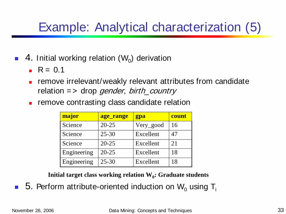
4. Initial working relation (W0) derivationR = 0.1remove irrelevant/weakly relevant attributes from candidate relation => drop gender, birth_countryremove contrasting class candidate relation

5. Perform attribute-oriented induction on W0 using Ti

major age_range gpa countScience 20-25 Very_good 16Science 25-30 Excellent 47Science 20-25 Excellent 21Engineering 20-25 Excellent 18Engineering 25-30 Excellent 18

Initial target class working relation W0: Graduate students








Discussion

Summary

Mining Class Comparisons

Comparison: Comparing two or more classes

Method:

Partition the set of relevant data into the target class and thecontrasting class(es)

Generalize both classes to the same high level concepts

Compare tuples with the same high level descriptions

Present for every tuple its description and two measures

support - distribution within single class

comparison - distribution between classes

Highlight the tuples with strong discriminant features

Relevance Analysis:

Find attributes (features) which best distinguish different classes


Example: Analytical comparison

TaskCompare graduate and undergraduate students using discriminant rule.DMQL query

use Big_University_DBmine comparison as “grad_vs_undergrad_students”in relevance to name, gender, major, birth_place, birth_date, residence, phone#, gpafor “graduate_students”where status in “graduate”versus “undergraduate_students”where status in “undergraduate”analyze count%from student


Example: Analytical comparison (2)

Givenattributes name, gender, major, birth_place, birth_date, residence, phone# and gpaGen(ai) = concept hierarchies on attributes ai

Ui = attribute analytical thresholds for attributes ai

Ti = attribute generalization thresholds for attributes ai

R = attribute relevance threshold



1. Data collectiontarget and contrasting classes

2. Attribute relevance analysisremove attributes name, gender, major, phone#

3. Synchronous generalizationcontrolled by user-specified dimension thresholdsprime target and contrasting class(es) relations/cuboids



Birth_country Age_range Gpa Count%Canada 20-25 Good 5.53%Canada 25-30 Good 2.32%Canada Over_30 Very_good 5.86%… … … …Other Over_30 Excellent 4.68%

Prime generalized relation for the target class: Graduate students

Birth_country Age_range Gpa Count%Canada 15-20 Fair 5.53%Canada 15-20 Good 4.53%… … … …Canada 25-30 Good 5.02%… … … …Other Over_30 Excellent 0.68%

Prime generalized relation for the contrasting class: Undergraduate students



4. Drill down, roll up and other OLAP operations on target and contrasting classes to adjust levels of abstractions of resulting description

5. Presentationas generalized relations, crosstabs, bar charts, pie charts, or rulescontrasting measures to reflect comparison between target and contrasting classes

e.g. count%


Quantitative Discriminant Rules

Cj = target classqa = a generalized tuple covers some tuples of class

but can also cover some tuples of contrasting classd-weight

range: [0, 1]

quantitative discriminant rule form

∑=

∈

∈=− m

iia

ja

)Ccount(q

)Ccount(qweightd

1

d_weight]:[dX)condition(ss(X)target_claX, ⇐∀


Example: Quantitative Discriminant Rule

Quantitative discriminant rule

where 90/(90+210) = 30%

Status Birth_country Age_range Gpa Count

Graduate Canada 25-30 Good 90

Undergraduate Canada 25-30 Good 210

Count distribution between graduate and undergraduate students for a generalized tuple

%]30:["")("3025")(_"")(_)(_,

dgoodXgpaXrangeageCanadaXcountrybirthXstudentgraduateX

=∧−=∧=⇐∀


Class Description

Quantitative characteristic rule

necessaryQuantitative discriminant rule

sufficientQuantitative description rule

necessary and sufficient]w:d,w:[t...]w:d,w:[t nn111 ′∨∨′

⇔∀(X)condition(X)condition

ss(X)target_claX,n

d_weight]:[dX)condition(ss(X)target_claX, ⇐∀

t_weight]:[tX)condition(ss(X)target_claX, ⇒∀


Example: Quantitative Description Rule

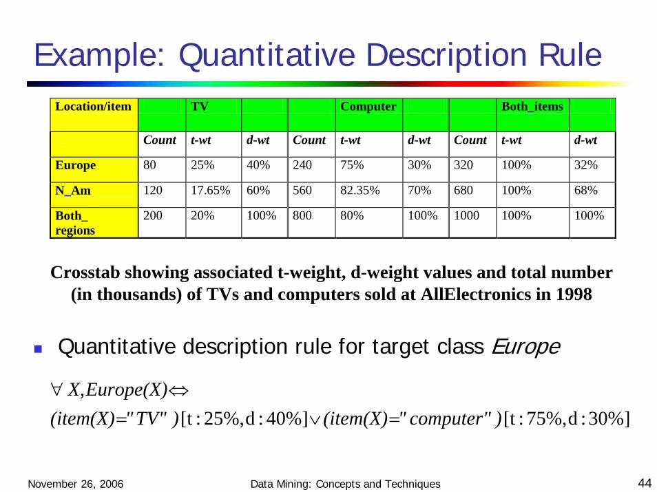
Quantitative description rule for target class Europe

Location/item TV Computer Both_items

Count t-wt d-wt Count t-wt d-wt Count t-wt d-wt

Europe 80 25% 40% 240 75% 30% 320 100% 32%

N_Am 120 17.65% 60% 560 82.35% 70% 680 100% 68%

Both_ regions

200 20% 100% 800 80% 100% 1000 100% 100%

Crosstab showing associated t-weight, d-weight values and total number (in thousands) of TVs and computers sold at AllElectronics in 1998

30%]:d75%,:[t40%]:d25%,:[t )computer""(item(X))TV""(item(X)Europe(X)X,

=∨=⇔∀


Mining Complex Data Objects: Generalization of Structured Data

Set-valued attributeGeneralization of each value in the set into its corresponding higher-level concepts

Derivation of the general behavior of the set, such as the number of elements in the set, the types or value ranges in the set, or the weighted average for numerical data

E.g., hobby = {tennis, hockey, chess, violin, nintendo_games} generalizes to {sports, music, video_games}

List-valued or a sequence-valued attributeSame as set-valued attributes except that the order of the elements in the sequence should be observed in the generalization


Generalizing Spatial and Multimedia Data

Spatial data:Generalize detailed geographic points into clustered regions, such as business, residential, industrial, or agricultural areas, according to land usageRequire the merge of a set of geographic areas by spatial operations

Image data:

Extracted by aggregation and/or approximation

Size, color, shape, texture, orientation, and relative positionsand structures of the contained objects or regions in the image

Music data:

Summarize its melody: based on the approximate patterns that repeatedly occur in the segment

Summarized its style: based on its tone, tempo, or the major musical instruments played


Summary

Concept description: characterization and discrimination

OLAP-based vs. attribute-oriented induction

Efficient implementation of AOI

Analytical characterization and comparison


Discussion

Incremental and parallel mining of description

Descriptive mining of complex types of data


References

Y. Cai, N. Cercone, and J. Han. Attribute-oriented induction in relational databases. In G. Piatetsky-Shapiro and W. J. Frawley, editors, Knowledge Discovery in Databases, pages 213-228. AAAI/MIT Press, 1991.S. Chaudhuri and U. Dayal. An overview of data warehousing and OLAP technology. ACM SIGMOD Record, 26:65-74, 1997C. Carter and H. Hamilton. Efficient attribute-oriented generalization for knowledge discovery from large databases. IEEE Trans. Knowledge and Data Engineering, 10:193-208, 1998.W. Cleveland. Visualizing Data. Hobart Press, Summit NJ, 1993.J. L. Devore. Probability and Statistics for Engineering and the Science, 4th ed. Duxbury Press, 1995.T. G. Dietterich and R. S. Michalski. A comparative review of selected methods for learning from examples. In Michalski et al., editor, Machine Learning: An Artificial Intelligence Approach, Vol. 1, pages 41-82. Morgan Kaufmann, 1983.J. Gray, S. Chaudhuri, A. Bosworth, A. Layman, D. Reichart, M. Venkatrao, F. Pellow, and H. Pirahesh. Data cube: A relational aggregation operator generalizing group-by, cross-tab and sub-totals. Data Mining and Knowledge Discovery, 1:29-54, 1997.J. Han, Y. Cai, and N. Cercone. Data-driven discovery of quantitative rules in relational databases. IEEE Trans. Knowledge and Data Engineering, 5:29-40, 1993.


References (cont.)

J. Han and Y. Fu. Exploration of the power of attribute-oriented induction in data mining. In U.M. Fayyad, G. Piatetsky-Shapiro, P. Smyth, and R. Uthurusamy, editors, Advances in Knowledge Discovery and Data Mining, pages 399-421. AAAI/MIT Press, 1996.R. A. Johnson and D. A. Wichern. Applied Multivariate Statistical Analysis, 3rd ed. Prentice Hall, 1992.E. Knorr and R. Ng. Algorithms for mining distance-based outliers in large datasets. VLDB'98, New York, NY, Aug. 1998.H. Liu and H. Motoda. Feature Selection for Knowledge Discovery and Data Mining. Kluwer Academic Publishers, 1998.R. S. Michalski. A theory and methodology of inductive learning. In Michalski et al., editor, Machine Learning: An Artificial Intelligence Approach, Vol. 1, Morgan Kaufmann, 1983.T. M. Mitchell. Version spaces: A candidate elimination approach to rule learning. IJCAI'97, Cambridge, MA.T. M. Mitchell. Generalization as search. Artificial Intelligence, 18:203-226, 1982.T. M. Mitchell. Machine Learning. McGraw Hill, 1997.J. R. Quinlan. Induction of decision trees. Machine Learning, 1:81-106, 1986.D. Subramanian and J. Feigenbaum. Factorization in experiment generation. AAAI'86, Philadelphia, PA, Aug. 1986.

Date post:	12-Apr-2018
Category:	Documents
Upload:	hoangngoc
View:	220 times
Download:	4 times

Data Mining: Concepts and Techniques -...

Documents