79
© Tan,Steinbach, Kumar Introduction to Data Mining 4/18/2004 1 Data Mining: Data Lecture Notes for Chapter 2 Introduction to Data Mining by Tan, Steinbach, Kumar

© Tan,Steinbach, Kumar Introduction to Data Mining 4/18/2004 1
Data Mining: Data
Lecture Notes for Chapter 2
Introduction to Data Miningby
Tan, Steinbach, Kumar

© Tan,Steinbach, Kumar Introduction to Data Mining 4/18/2004 2
What is Data?
Collection of data objects and their attributes
An attribute is a property or characteristic of an object
– Examples: eye color of a person, temperature, etc.
– Attribute is also known as variable, field, characteristic, or feature
A collection of attributes describe an object
– Object is also known as record, point, case, sample, entity, or instance
Tid Refund Marital Status
Taxable Income Cheat
1 Yes Single 125K No
2 No Married 100K No
3 No Single 70K No
4 Yes Married 120K No
5 No Divorced 95K Yes
6 No Married 60K No
7 Yes Divorced 220K No
8 No Single 85K Yes
9 No Married 75K No
10 No Single 90K Yes 10
Attributes
Objects

© Tan,Steinbach, Kumar Introduction to Data Mining 4/18/2004 5
Properties of Attribute Values
The type of an attribute depends on which of the following properties it possesses:– Distinctness: = – Order: < > – Addition: + - – Multiplication: * /
– Nominal attribute: distinctness– Ordinal attribute: distinctness & order– Interval attribute: distinctness, order & addition– Ratio attribute: all 4 properties
© Tan,Steinbach, Kumar Introduction to Data Mining 4/18/2004 6
Types of Attributes
There are different types of attributes– Nominal
Examples:
– Ordinal Examples:
– Interval Examples:
– Ratio Examples:

© Tan,Steinbach, Kumar Introduction to Data Mining 4/18/2004 7
Types of Attributes
There are different types of attributes– Nominal
Examples: ID numbers, eye color, zip codes
– Ordinal Examples: rankings (e.g., taste of potato chips on a scale
from 1-10), grades, height in {tall, medium, short}
– Interval Examples: calendar dates, temperatures in Celsius or
Fahrenheit.
– Ratio Examples: temperature in Kelvin, length, time, counts

© Tan,Steinbach, Kumar Introduction to Data Mining 4/18/2004 8
Example
Dec 3, 2000 ≠ Dec 24, 2000 Dec 3, 2000 <(=earlier than) Dec 24, 2000 Dec 24,2000 – Dec 3, 2000 = 21 days BUT: (Dec 24, 2000) / (Dec 3, 2000) = ???
-> Dates are interval attributes.

© Tan,Steinbach, Kumar Introduction to Data Mining 4/18/2004 9
Attribute Type
Description Examples Operations
Nominal The values of a nominal attribute are just different names, i.e., nominal attributes provide only enough information to distinguish one object from another. (=, )
zip codes, employee ID numbers, eye color, sex: {male, female}
mode, entropy, contingency correlation, 2 test
Ordinal The values of an ordinal attribute provide enough information to order objects. (<, >)
hardness of minerals, {good, better, best}, grades, street numbers
median, percentiles, rank correlation, run tests, sign tests
Interval For interval attributes, the differences between values are meaningful, i.e., a unit of measurement exists. (+, - )
calendar dates, temperature in Celsius or Fahrenheit
mean, standard deviation, Pearson's correlation
Ratio For ratio variables, both differences and ratios are meaningful. (*, /)
temperature in Kelvin, monetary quantities, counts, age, mass, length, electrical current
geometric mean, harmonic mean, percent variation
© Tan,Steinbach, Kumar Introduction to Data Mining 4/18/2004 10
Attribute Level
Transformation Comments
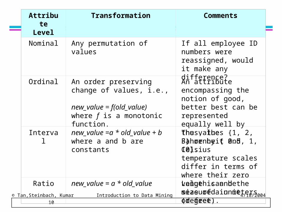
Nominal Any permutation of values If all employee ID numbers were reassigned, would it make any difference?
Ordinal An order preserving change of values, i.e., new_value = f(old_value) where f is a monotonic function.
An attribute encompassing the notion of good, better best can be represented equally well by the values {1, 2, 3} or by { 0.5, 1, 10}.
Interval new_value =a * old_value + b where a and b are constants
Thus, the Fahrenheit and Celsius temperature scales differ in terms of where their zero value is and the size of a unit (degree).
Ratio new_value = a * old_value Length can be measured in meters or feet.

© Tan,Steinbach, Kumar Introduction to Data Mining 4/18/2004 12
Types of data sets Record
– Data Matrix– Document Data– Transaction Data
Graph– World Wide Web– Molecular Structures
Ordered– Spatial Data– Temporal Data– Sequential Data– Genetic Sequence Data

© Tan,Steinbach, Kumar Introduction to Data Mining 4/18/2004 13
Record Data
Data that consists of a collection of records, each of which consists of a fixed set of attributes
Tid Refund Marital Status
Taxable Income Cheat
1 Yes Single 125K No
2 No Married 100K No
3 No Single 70K No
4 Yes Married 120K No
5 No Divorced 95K Yes
6 No Married 60K No
7 Yes Divorced 220K No
8 No Single 85K Yes
9 No Married 75K No
10 No Single 90K Yes 10

© Tan,Steinbach, Kumar Introduction to Data Mining 4/18/2004 14
Data Matrix
If data objects have the same fixed set of numeric attributes, then the data objects can be thought of as points in a multi-dimensional space, where each dimension represents a distinct attribute
Such data set can be represented by an m by n matrix, where there are m rows, one for each object, and n columns, one for each attribute
1.12.216.226.2512.65
1.22.715.225.2710.23
Thickness LoadDistanceProjection of y load
Projection of x Load
1.12.216.226.2512.65
1.22.715.225.2710.23
Thickness LoadDistanceProjection of y load
Projection of x Load

© Tan,Steinbach, Kumar Introduction to Data Mining 4/18/2004 16
Transaction Data
A special type of record data, where – each record (transaction) involves a set of items. – For example, consider a grocery store. The set of
products purchased by a customer during one shopping trip constitute a transaction, while the individual products that were purchased are the items.
TID Items
1 Bread, Coke, Milk
2 Beer, Bread
3 Beer, Coke, Diaper, Milk
4 Beer, Bread, Diaper, Milk
5 Coke, Diaper, Milk

© Tan,Steinbach, Kumar Introduction to Data Mining 4/18/2004 17
Graph Data
Examples: Generic graph, HTML Links, Benzene Molecule: C6H6
5
2
1 2
5
<a href="papers/papers.html#bbbb">Data Mining </a><li><a href="papers/papers.html#aaaa">Graph Partitioning </a><li><a href="papers/papers.html#aaaa">Parallel Solution of Sparse Linear System of Equations </a><li><a href="papers/papers.html#ffff">N-Body Computation and Dense Linear System Solvers

© Tan,Steinbach, Kumar Introduction to Data Mining 4/18/2004 19
Ordered Data
Genomic sequence data
GGTTCCGCCTTCAGCCCCGCGCCCGCAGGGCCCGCCCCGCGCCGTCGAGAAGGGCCCGCCTGGCGGGCGGGGGGAGGCGGGGCCGCCCGAGCCCAACCGAGTCCGACCAGGTGCCCCCTCTGCTCGGCCTAGACCTGAGCTCATTAGGCGGCAGCGGACAGGCCAAGTAGAACACGCGAAGCGCTGGGCTGCCTGCTGCGACCAGGG

© Tan,Steinbach, Kumar Introduction to Data Mining 4/18/2004 20
Ordered Data
Spatio-Temporal Data
Average Monthly Temperature of land and ocean

© Tan,Steinbach, Kumar Introduction to Data Mining 4/18/2004 21
Data Quality
What kinds of data quality problems? How to detect problems with the data? What can we do about these problems?
Examples of data quality problems: – Noise, outliers, and inconsistencies – missing values – duplicate data
Tid Refund Marital Status
Taxable Income Cheat
1 Yes ??? 125K No
2 No Married 100K No
3 No Single 100000K No
4 Yes Married 120K No
5 No Divorced 95K ???
6 No Single 85K Yes
7 No Single 85K Yes
8 No Single 85K Yes
9 No Single 85K Yes
10 No Single 85K Yes 10

© Tan,Steinbach, Kumar Introduction to Data Mining 4/18/2004 22
Noise
Noise refers to modification of original values– Examples: distortion of a person’s voice when talking
on a poor phone and “snow” on television screen
Sine Wave + Noise Image + Salt & Pepper Noise

© Tan,Steinbach, Kumar Introduction to Data Mining 4/18/2004 23
Noise
Noise refers to modification of original valuesProblem: Signal might be covered by noise
Sine Wave + Noise Image + Salt & Pepper Noise

© Tan,Steinbach, Kumar Introduction to Data Mining 4/18/2004 24
Outliers
Outliers are data objects with characteristics that are considerably different than most of the other data objects in the data set
Problem: many statistics (e.g. mean, min., max., etc.) are strongly affected by outlier

Lecture 2 – January 17, 2008Jon Doyle © 2008 25NC STATE UNIVERSITY
(C) Vipin Kumar, Parallel Issues in Data Mining, VECPAR 2002
25
Data Inconsistencies Single-source errors, e.g. repeated transactions, or
communication errors Data integration difficulties
Need not involve errors– Different representations (numeric precision)– Different scales or units
Conflicting meanings in different schema– Patient medications lists– Street address
How to resolve? Select one of the conflicting values Replace with estimated value

© Tan,Steinbach, Kumar Introduction to Data Mining 4/18/2004 32
Important Characteristics of Structured Data
– Dimensionality Curse of Dimensionality
– Sparsity Only presence counts
– Resolution Patterns depend on the scale

© Tan,Steinbach, Kumar Introduction to Data Mining 4/18/2004 33
Data Preprocessing
Aggregation Sampling Dimensionality Reduction Feature subset selection Feature creation Discretization and Binarization

© Tan,Steinbach, Kumar Introduction to Data Mining 4/18/2004 34
Aggregation
Combining two or more attributes (or objects) into a single attribute (or object)
Purpose– Data reduction
Reduce the number of attributes or objects
– Change of scale Cities aggregated into regions, states, countries, etc
– More “stable” data Aggregated data tends to have less variability

© Tan,Steinbach, Kumar Introduction to Data Mining 4/18/2004 35
Aggregation
Standard Deviation of Average Monthly Precipitation
Standard Deviation of Average Yearly Precipitation
Variation of Precipitation in Australia

Lecture 2 – January 17, 2008Jon Doyle © 2008 36NC STATE UNIVERSITY
(C) Vipin Kumar, Parallel Issues in Data Mining, VECPAR 2002
36
Aggregation using data cubes OLAP (online analytical
processing) often based on data cubes A multidimensional data
model akin to tables and spreadsheets
A sales data cube, for example, models data and allows viewing in multiple dimensions Dimension tables, such as item (item_name, brand,
type), or time(day, week, month, quarter, year) Fact table contains measures (such as dollars_sold)
and keys to each of the related dimension tables
Prod
uct
Region
Month

Lecture 2 – January 17, 2008Jon Doyle © 2008 37NC STATE UNIVERSITY
(C) Vipin Kumar, Parallel Issues in Data Mining, VECPAR 2002
37
A sample data cubeTotal annual salesof TV in U.S.A.Date
Produ
ct
Cou
ntrysum
sum TV
VCRPC
1Qtr 2Qtr 3Qtr 4Qtr
U.S.A
Canada
Mexico
sum

Lecture 2 – January 17, 2008Jon Doyle © 2008 38NC STATE UNIVERSITY
(C) Vipin Kumar, Parallel Issues in Data Mining, VECPAR 2002
38
Fact Table and Dimension Tables

Lecture 2 – January 17, 2008Jon Doyle © 2008 39NC STATE UNIVERSITY
(C) Vipin Kumar, Parallel Issues in Data Mining, VECPAR 2002
39
Typical OLAP operations Roll up (drill-up): summarize data
by climbing up hierarchy or by dimension reduction Drill down (roll down): reverse of roll-up
from higher level summary to lower level summary or detailed data, or introducing new dimensions
Slice and dice: project and select
Pivot (rotate): reorient the cube, visualization, 3D to series of 2D
planes. Other operations
drill across: involving (across) more than one fact table
drill through: through the bottom level of the cube to its back-end relational tables (using SQL)
Lecture 2 – January 17, 2008Jon Doyle © 2008 40NC STATE UNIVERSITY
(C) Vipin Kumar, Parallel Issues in Data Mining, VECPAR 2002
40
Analysis-driven aggregation Aggregate specific dimensions until
desired size obtained Different dimensions yield different
sizes Use the smallest size cube that leaves
intact the dimensions one is trying to analyze

© Tan,Steinbach, Kumar Introduction to Data Mining 4/18/2004 41
Sampling Sampling is the main technique employed for data selection.
– often used for both the preliminary investigation of the data and the final data analysis.
Statisticians sample because obtaining the entire set of data of interest is too expensive or time consuming.
Sampling is used in data mining because processing the entire set of data of interest is too expensive or time consuming.
Key principle for effective sampling: – a sample will work almost as well as using the entire data sets, if the
sample is representative– A sample is representative if it has approximately the same property (of
interest) as the original set of data

© Tan,Steinbach, Kumar Introduction to Data Mining 4/18/2004 42
Sample Size
8000 points 2000 Points 500 Points

© Tan,Steinbach, Kumar Introduction to Data Mining 4/18/2004 43
Sample Size What sample size is necessary to get at least one
object from each of 10 groups.

© Tan,Steinbach, Kumar Introduction to Data Mining 4/18/2004 44
Types of Sampling
Simple Random Sampling– There is an equal probability of selecting any particular item
Sampling without replacement– As each item is selected, it is removed from the population
Sampling with replacement– Objects are not removed from the population as they are
selected for the sample. In sampling with replacement, the same object can be picked up more
than once
Stratified sampling– Split the data into several partitions; then draw random samples
from each partition

© Tan,Steinbach, Kumar Introduction to Data Mining 4/18/2004 45
Grid-based Sampling
Fixed Grid:
Flexible Grid:

© Tan,Steinbach, Kumar Introduction to Data Mining 4/18/2004 46
Curse of Dimensionality
When dimensionality increases, data becomes increasingly sparse in the space that it occupies
How many grid points do you need for a 10 dimensional cube?

© Tan,Steinbach, Kumar Introduction to Data Mining 4/18/2004 47
Curse of Dimensionality
Example (Richard Bellman): 100 evenly-spaced sample points suffice to sample a unit interval with no more than 0.01 distance between points.
How many points with a spacing of 0.01 between adjacent points do you need for an equivalent sampling of a 10-dimensional unit hypercube?
Answer: 10010 = 1020 that is a factor of 1018 more!

© Tan,Steinbach, Kumar Introduction to Data Mining 4/18/2004 48
Curse of Dimensionality
When dimensionality increases, data becomes increasingly sparse in the space that it occupies
0)()(
n
hypercubeVolumeehyperspherVolume
© Tan,Steinbach, Kumar Introduction to Data Mining 4/18/2004 49
Curse of Dimensionality
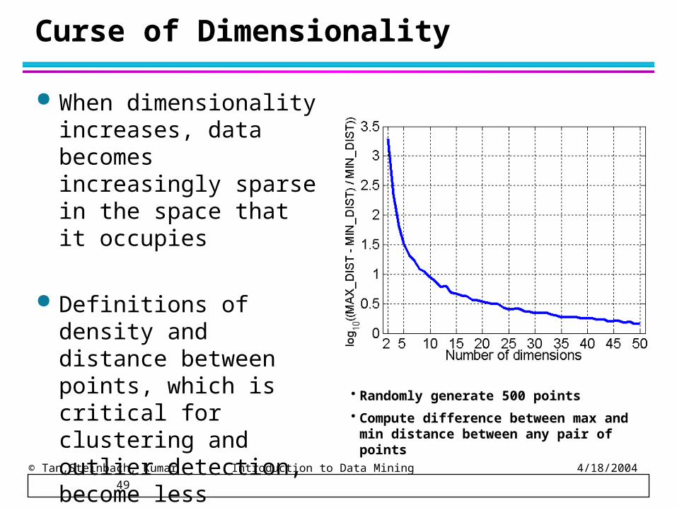
When dimensionality increases, data becomes increasingly sparse in the space that it occupies
Definitions of density and distance between points, which is critical for clustering and outlier detection, become less meaningful • Randomly generate 500 points
• Compute difference between max and min distance between any pair of points

© Tan,Steinbach, Kumar Introduction to Data Mining 4/18/2004 50
Dimensionality Reduction
Purposes:– Avoid curse of dimensionality– Reduce amount of time and memory required by data
mining algorithms– Allow data to be more easily visualized– May help to eliminate irrelevant features or reduce
noise
Techniques– Principle Component Analysis (PCA)– Feature subset selection

© Tan,Steinbach, Kumar Introduction to Data Mining 4/18/2004 51
Dimensionality Reduction: Principle Componenent Analysis (PCA)
Goal is to find a projection that captures the largest amount of variation in data

© Tan,Steinbach, Kumar Introduction to Data Mining 4/18/2004 52
Dimensionality Reduction: Principle Componenent Analysis (PCA)
Goal is to find a projection that captures the largest amount of variation in data
v1
© Tan,Steinbach, Kumar Introduction to Data Mining 4/18/2004 53
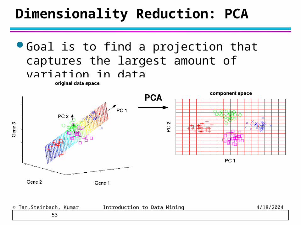
Dimensionality Reduction: PCA
Goal is to find a projection that captures the largest amount of variation in data

© Tan,Steinbach, Kumar Introduction to Data Mining 4/18/2004 54
How PCA Works
Subtract mean (centering) Find the eigenvectors of the covariance matrix The eigenvectors are the principle components
PC1
PC2
= 0

© Tan,Steinbach, Kumar Introduction to Data Mining 4/18/2004 55 55
Covariance of Two Vectors, cov(p,q)
1 2 1 2( , ,...., ) and ( , ,...., )d dd dp p p p q q q q
1
1 d
kk
p pd
Mean of attributes
1
1cov( , ) ( )( )1
d
pq k kk
p q s p p q qd
Your text-book definition:
cov( , ) [( ( ))( ( )) ]Tp q E p E p q E q
Better definition:
E is the Expected values of a random variable.

© Tan,Steinbach, Kumar Introduction to Data Mining 4/18/2004 56 56
Covariance, or Dispersion Matrix,
1 11 12 1
1 2
( , ,...., ) .....
( , ,...., )
dd
dN N N Nd
P p p p
P p p p
1 1 1 2 1
2 1 2 2 21 2
1 2
cov( , ) cov( , ) ... cov( , )cov( , ) cov( , ) ... cov( , )
( , ,..., )... ... ... ...
cov( , ) cov( , ) ... cov( , )
N
NN
N N N N
P P P P P PP P P P P P
P P P
P P P P P P
N points in d-dimensional space:
The covariance, or dispersion matrix:
The inverse, Σ-1, is concentration matrix or precision matrix

© Tan,Steinbach, Kumar Introduction to Data Mining 4/18/2004 57 57
Mathematics behind PCA
Singular Value Decomposition (SVD)
The technique underlying PCA analysis
∑ U U d x d
Eigenvalues (diagonal matrix)
…PC1PCk
Eigenvectors/Principal Components (orthonormal)
Sum of k eigenvaluesSum of all eigenvalues
Preserved variability =
with k dimensions
T
1cov( ) ( )T Td d m d m d m d m
m d
X X X x x
Covariance matrix Column meansCovariance matrix
1 2 ... ... 0k d
1 1
1
trace ( )
k k
i ii id
ii
Singular Value Decomposition (SVD)
The technique underlying PCA analysis
∑ U U d x d
Eigenvalues (diagonal matrix)
…PC1PCk
Eigenvectors/Principal Components (orthonormal)
Sum of k eigenvaluesSum of all eigenvalues
Preserved variability =
with k dimensions
T

© Tan,Steinbach, Kumar Introduction to Data Mining 4/18/2004 58
Eigenfaces
Transform images into a vector of size N andbuild data matrix X.
Subtract average face
-
© Tan,Steinbach, Kumar Introduction to Data Mining 4/18/2004 59
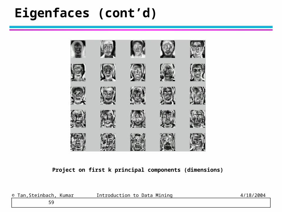
Eigenfaces (cont’d)
Project on first k principal components (dimensions)
© Tan,Steinbach, Kumar Introduction to Data Mining 4/18/2004 60
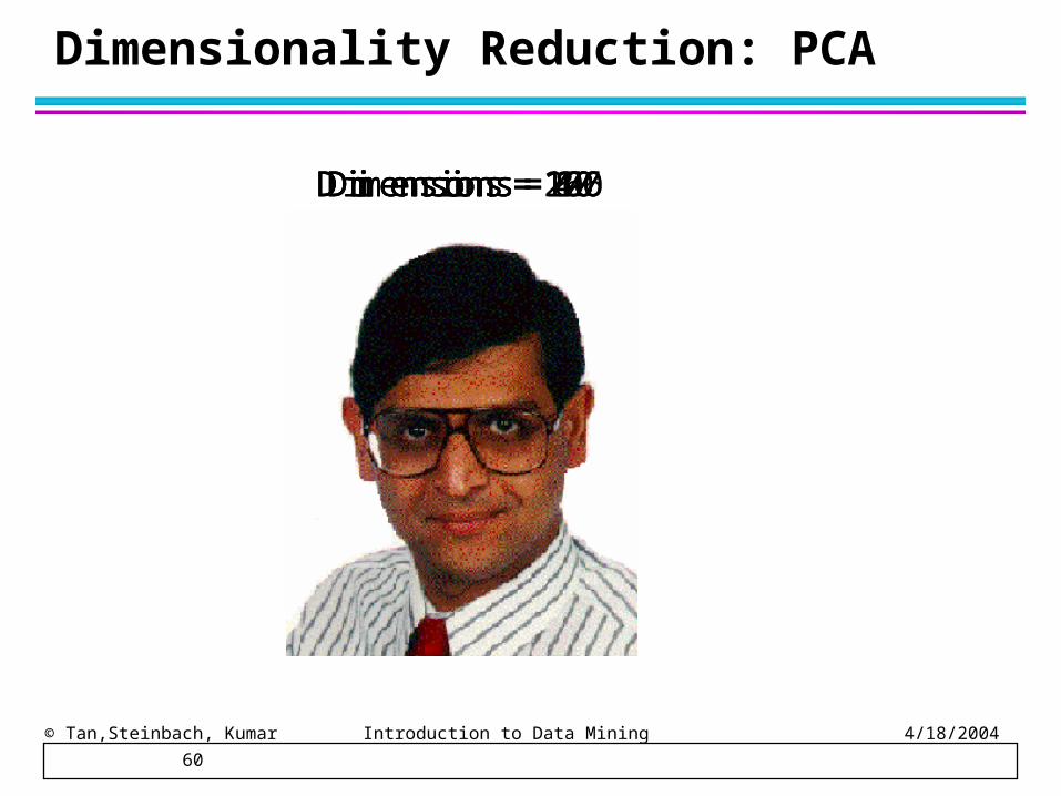
Dimensions = 10Dimensions = 40Dimensions = 80Dimensions = 120Dimensions = 160Dimensions = 206
Dimensionality Reduction: PCA

© Tan,Steinbach, Kumar Introduction to Data Mining 4/18/2004 61
Feature Subset Selection
Another way to reduce dimensionality of data
Redundant features – duplicate much or all of the information contained in
one or more other attributes– Example: purchase price of a product and the amount
of sales tax paid
Irrelevant features– contain no information that is useful for the data
mining task at hand– Example: students' ID is often irrelevant to the task of
predicting students' GPA

© Tan,Steinbach, Kumar Introduction to Data Mining 4/18/2004 62
Feature Subset Selection Techniques
Brute-force approach: Try all possible feature subsets as input to data
mining algorithm
Embedded approaches: Feature selection occurs naturally as part of the
data mining algorithm

© Tan,Steinbach, Kumar Introduction to Data Mining 4/18/2004 63
Feature Subset Selection
Filter approaches: Features are selected before data mining algorithm is run
Wrapper approaches: Use the data mining algorithm as a black box to find best subset of attributes

© Tan,Steinbach, Kumar Introduction to Data Mining 4/18/2004 64
Feature Creation
Create new attributes that can capture the important information in a data set much more efficiently than the original attributes
Three general methodologies:– Feature Extraction
domain-specific
– Mapping Data to New Space– Feature Construction
combining features

© Tan,Steinbach, Kumar Introduction to Data Mining 4/18/2004 65
Mapping Data to a New Space
Two Sine Waves Two Sine Waves + Noise Frequency
Fourier transform Wavelet transform

© Tan,Steinbach, Kumar Introduction to Data Mining 4/18/2004 68
Attribute Transformation
A function that maps the entire set of values of a given attribute to a new set of values such that each old value can be identified with one of the new values– Simple functions: xk, log(x),
ex, |x|– Standardization and
Normalization
Scatterplot of areas and population ofthe states in the world. [WIKI]

© Tan,Steinbach, Kumar Introduction to Data Mining 4/18/2004 69
Discretization Without Using Class Labels
Data Equal interval width
Equal frequency K-means
© Tan,Steinbach, Kumar Introduction to Data Mining 4/18/2004 70
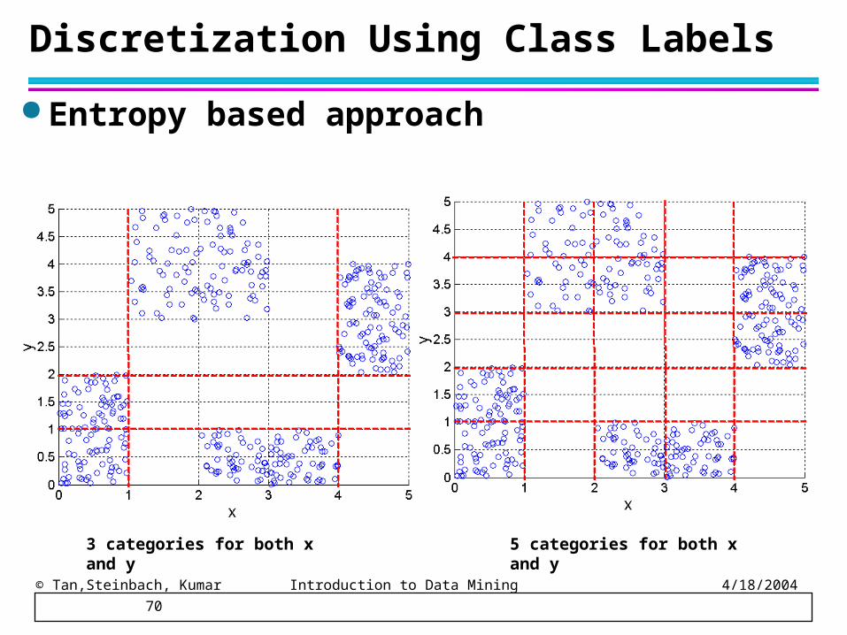
Discretization Using Class Labels Entropy based approach
3 categories for both x and y 5 categories for both x and y

© Tan,Steinbach, Kumar Introduction to Data Mining 4/18/2004 71 71
Bottom-up approach: Data Methods
Q1: What are the individual points?Data Question:
Q2: How to “compare” two points?Similarity/Dissimilarity/Distance Measure Question:
Lecture focus

© Tan,Steinbach, Kumar Introduction to Data Mining 4/18/2004 72
Similarity and Dissimilarity
Similarity– Numerical measure of how alike two data objects are.– Is higher when objects are more alike.– Often falls in the range [0,1]
Dissimilarity– Numerical measure of how different are two data
objects– Lower when objects are more alike– Minimum dissimilarity is often 0– Upper limit varies
Proximity refers to a similarity or dissimilarity

© Tan,Steinbach, Kumar Introduction to Data Mining 4/18/2004 73
Similarity/Dissimilarity for Simple Attributes
p and q are the attribute values for two data objects.

© Tan,Steinbach, Kumar Introduction to Data Mining 4/18/2004 74 74
Euclidean Distance 2
1
( , ) ( )d
j jj
d p q p q
Standardization is necessary, if scales differ.
1 2( , ,...., ) ddp p p p
1
1 d
kk
p pd
Mean of attributes Standard deviation of attributes
2
1
1 ( )1
d
p kk
s p pd
Ex: ( , )p age salary
Standardized/Normalized Vector
1 2( , ,..., ) ddnew
p p p p
p pp p p pp pps s s s
01
new
new
p
ps

© Tan,Steinbach, Kumar Introduction to Data Mining 4/18/2004 75
Minkowski Distance
Minkowski Distance is a generalization of Euclidean Distance
Where r is a parameter, n is the number of dimensions
(attributes) and pk and qk are, respectively, the kth attributes (components) or data objects p and q.
rn
k
rkk qpdist
1
1)||(
unit circles with various values of r [Wikipedia]
© Tan,Steinbach, Kumar Introduction to Data Mining 4/18/2004 76
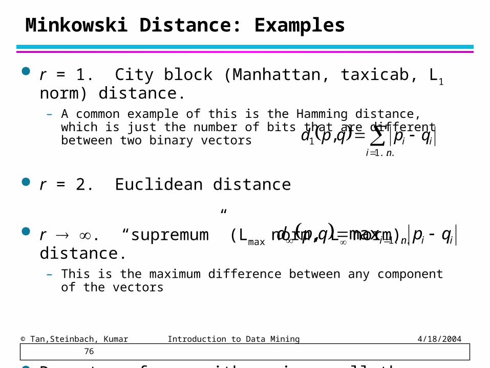
Minkowski Distance: Examples
r = 1. City block (Manhattan, taxicab, L1 norm) distance. – A common example of this is the Hamming distance, which is just the
number of bits that are different between two binary vectors
r = 2. Euclidean distance
r . “supremum” (Lmax norm, L norm) distance. – This is the maximum difference between any component of the vectors
Do not confuse r with n, i.e., all these distances are defined for all numbers of dimensions.
ni
ii qpqpd...1
1 ,
iini qpqpd ...1max,

© Tan,Steinbach, Kumar Introduction to Data Mining 4/18/2004 77
Minkowski Distance
Distance Matrix
point x yp1 0 2p2 2 0p3 3 1p4 5 1
L1 p1 p2 p3 p4p1 0 4 4 6p2 4 0 2 4p3 4 2 0 2p4 6 4 2 0
L2 p1 p2 p3 p4p1 0 2.828 3.162 5.099p2 2.828 0 1.414 3.162p3 3.162 1.414 0 2p4 5.099 3.162 2 0
L p1 p2 p3 p4p1 0 2 3 5p2 2 0 1 3p3 3 1 0 2p4 5 3 2 0

© Tan,Steinbach, Kumar Introduction to Data Mining 4/18/2004 78
Mahalanobis Distance
Tqpqpqpsmahalanobi )()(),( 1
is the covariance matrix of the input data X
n
ikikjijkj XXXX
n 1, ))((
11

© Tan,Steinbach, Kumar Introduction to Data Mining 4/18/2004 79
Mahalanobis Distance
Tqpqpqpsmahalanobi )()(),( 1
is the covariance matrix of the input data X
n
ikikjijkj XXXX
n 1, ))((
11

© Tan,Steinbach, Kumar Introduction to Data Mining 4/18/2004 80
Mahalanobis Distance
Covariance Matrix:
3.02.02.03.0
B
A
C
A: (0.5, 0.5)B: (0, 1)C: (1.5, 1.5)
Mahal(A,B) = 5Mahal(A,C) = 4

© Tan,Steinbach, Kumar Introduction to Data Mining 4/18/2004 81
Common Properties of a Distance
Distances, such as the Euclidean distance, have some well known properties.
1. d(p, q) 0 for all p and q and d(p, q) = 0 only if p = q. (Positive definiteness)
2. d(p, q) = d(q, p) for all p and q. (Symmetry)3. d(p, r) d(p, q) + d(q, r) for all points p, q, and r.
(Triangle Inequality)
where d(p, q) is the distance (dissimilarity) between points (data objects), p and q.
A distance that satisfies these properties is a metric
© Tan,Steinbach, Kumar Introduction to Data Mining 4/18/2004 82 82
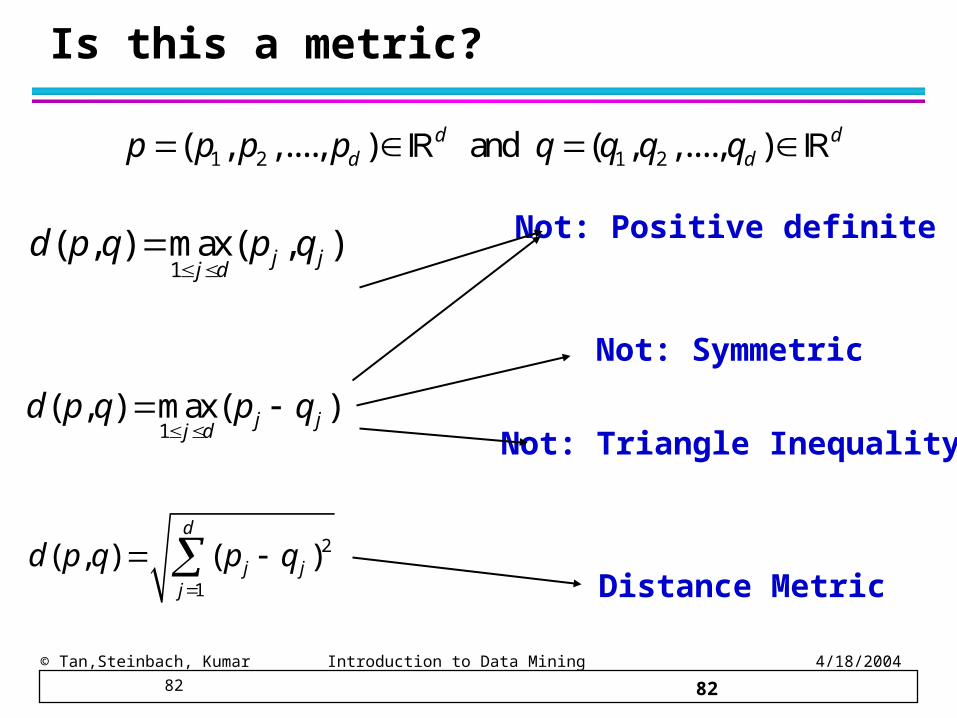
Is this a metric?
Not: Positive definite
Not: Symmetric
Not: Triangle Inequality
1( , ) max( , )j jj d
d p q p q
Distance Metric
1 2 1 2( , ,...., ) and ( , ,...., )d dd dp p p p q q q q
1( , ) max( )j jj d
d p q p q
2
1
( , ) ( )d
j jj
d p q p q

© Tan,Steinbach, Kumar Introduction to Data Mining 4/18/2004 83
Common Properties of Similarity
Similarities also have some well known properties.
1. s(p, q) = 1 (or maximum similarity) only if p = q.
2. s(p, q) = s(q, p) for all p and q. (Symmetry)
where s(p, q) is the similarity between points (data objects), p and q.

© Tan,Steinbach, Kumar Introduction to Data Mining 4/18/2004 84
Similarity Between Binary Vectors Common situation is that objects, p and q, have only
binary attributes
Compute similarities using the following quantitiesM01 = the number of attributes where p was 0 and q was 1M10 = the number of attributes where p was 1 and q was 0M00 = the number of attributes where p was 0 and q was 0M11 = the number of attributes where p was 1 and q was 1
Simple Matching and Jaccard Coefficients SMC = number of matches / number of attributes
= (M11 + M00) / (M01 + M10 + M11 + M00)
J = number of 11 matches / number of not-both-zero attributes values = (M11) / (M01 + M10 + M11)

© Tan,Steinbach, Kumar Introduction to Data Mining 4/18/2004 85
SMC versus Jaccard: Example
p = 1 0 0 0 0 0 0 0 0 0 q = 0 0 0 0 0 0 1 0 0 1
M01 = 2 (the number of attributes where p was 0 and q was 1)M10 = 1 (the number of attributes where p was 1 and q was 0)M00 = 7 (the number of attributes where p was 0 and q was 0)M11 = 0 (the number of attributes where p was 1 and q was 1)
SMC = (M11 + M00)/(M01 + M10 + M11 + M00) = (0+7) / (2+1+0+7) = 0.7
J = (M11) / (M01 + M10 + M11) = 0 / (2 + 1 + 0) = 0

© Tan,Steinbach, Kumar Introduction to Data Mining 4/18/2004 86
Cosine Similarity If d1 and d2 are two document vectors, then
cos( d1, d2 ) = (d1 d2) / ||d1|| ||d2|| , where indicates vector dot product and || d || is the length of vector d.
Example:
d1 = 3 2 0 5 0 0 0 2 0 0 d2 = 1 0 0 0 0 0 0 1 0 2
d1 d2= 3*1 + 2*0 + 0*0 + 5*0 + 0*0 + 0*0 + 0*0 + 2*1 + 0*0 + 0*2 = 5
||d1|| = (3*3+2*2+0*0+5*5+0*0+0*0+0*0+2*2+0*0+0*0)0.5 = (42) 0.5 = 6.481
||d2|| = (1*1+0*0+0*0+0*0+0*0+0*0+0*0+1*1+0*0+2*2) 0.5 = (6) 0.5 = 2.245
cos( d1, d2 ) = .3150

© Tan,Steinbach, Kumar Introduction to Data Mining 4/18/2004 88
Correlation
Correlation measures the linear relationship between objects
To compute correlation, we standardize data objects, p and q, and then take their dot product
)(/))(( pstdpmeanpp kk
)(/))(( qstdqmeanqq kk
qpqpncorrelatio ),(

© Tan,Steinbach, Kumar Introduction to Data Mining 4/18/2004 89
Visually Evaluating Correlation
Scatter plots showing the similarity from –1 to 1.

© Tan,Steinbach, Kumar Introduction to Data Mining 4/18/2004 90
Warning!!! Correlation can be tricky
Scatter plots showing the similarity from –1 to 1.
Guess the correlation coefficient

© Tan,Steinbach, Kumar Introduction to Data Mining 4/18/2004 91
General Approach for Combining Similarities
Sometimes attributes are of many different types, but an overall similarity is needed.

© Tan,Steinbach, Kumar Introduction to Data Mining 4/18/2004 92
Using Weights to Combine Similarities
May not want to treat all attributes the same.– Use weights wk which are between 0 and 1 and sum
to 1.
© Tan,Steinbach, Kumar Introduction to Data Mining 4/18/2004 93
Thank You!


