29

1

Data Mining ProjectPredicting Groundwater Fluctuations in France
Martin Mugnier, Tong Chen
February 20, 2019
Contents1 Introduction 3
2 Data description 42.1 Data collection . . . . . . . . . . . . . . . . . . . . . . . . . . . . . . . . . . . . . 42.2 Some descriptive statistics . . . . . . . . . . . . . . . . . . . . . . . . . . . . . . . 42.3 The data selection procedure . . . . . . . . . . . . . . . . . . . . . . . . . . . . . 6
3 Analysis of individual series 93.1 Fourier Method . . . . . . . . . . . . . . . . . . . . . . . . . . . . . . . . . . . . . 93.2 Random Forest . . . . . . . . . . . . . . . . . . . . . . . . . . . . . . . . . . . . . 113.3 GAM . . . . . . . . . . . . . . . . . . . . . . . . . . . . . . . . . . . . . . . . . . 113.4 Comparison . . . . . . . . . . . . . . . . . . . . . . . . . . . . . . . . . . . . . . . 13
4 An attempt at global modelling for ground water fluctuations 144.1 Methodology . . . . . . . . . . . . . . . . . . . . . . . . . . . . . . . . . . . . . . 144.2 Results from the training and optimization step (daily variations) . . . . . . . . . 154.3 Performances on new data . . . . . . . . . . . . . . . . . . . . . . . . . . . . . . . 184.4 Results for next week normalized level and weekly variations . . . . . . . . . . . 19
5 Expert aggregation 20
6 Discussion of results and conclusion 22
2

1 IntroductionGroundwater is an essential resource for human life and the development of human activities.Understanding the fluctuations in our reserves and the phenomena at work is therefore essentialto better manage and anticipate the quantities of water available. In this project, we aim to builda forecasting model for predicting fluctuations of the water level in the main groundwater reservesin France. Although most of these fluctuations are prone to be explained by specific locationfactors and physics conditions that are not always approachable by data, we suspect that somefactors of influence should be common to every well conditional on some variables. For instance,you may think of meteorological data (such as rainfall, snowfall), geological data (altitude, soilcomposition) or even the uses made of each well (industrial, agricultural, animal husbandry,supply). For instance, conditioning on altitude might reveal common responses and causal effectof rainfalls on the water levels. Many papers have investigated the problem of predicting waterfluctuations : some using classic tools from physic simulation models (Van Asch and Buma,1997) and other using similar data than our and drawing from basic statistics (Abiyea et al.,2018) to very involved models including Artificial Neural Networks (ANNs) (Sujay Raghavendraand Deka, 2015)(Shamsuddin et al., 2017)(Vetrivel and Elangovan, 2016) or wavelets augmentedmodels (Zare and Koch, 2018). See Shiri et al. (2013) for a comparison. While most of theresearch comes from developing countries and most of articles focus on very precise wells withmany measurements, a few if none (to our knowledge) have tackled the issue globally for France,where a lot of data is publicly available. The main goal of this study is thus double : i) to ratio-nalize these possible non-linear interactions within a model which could help to understand whichfactors play a role in groundwater fluctuations, ii) to investigate the extent to which machinelearning algorithms can yield good prediction using only public available data. More precisely,we are interested in the best way to gives predictions about a water level metric (profondeur rel-ative, in meters) at time t ∈ [T ] = {1, . . . , T} for site i ∈ [N ] = {1, . . . , N} given all informationavailable. The latter can be relative to that precise well but potentially to every other wells.
There are more than 4,000 water wells spread over the country and for which the Ministry ofEcological and Solidarity Transition publishes very precise measurements on a daily basis. Ourmethodology decomposes in :
i. collecting enough public data that can have a fairly strong predictive power on our explainedvariable ;
ii. building the most relevant model in a context of bi-dimensional observations (sites andtime).
These tasks involve several very important intermediate steps, such as on the one hand todefine exactly the most relevant variable to be predicted and on the other hand to address theissue of aggregating heterogenous time-dependent series in a context of panel data (several wellsare observed on a daily basis). For instance should we consider only several wells individuallyleaving aside the huge amount of information brought by all the wells or should we aggregateinformation to build a unique general model ? Note that maybe a proper combination of bothkind of models, in the spirit of expert aggregation techniques, could perform well. Throughoutthe paper, we will describe all of our choices and results.
The remaining is organized as follows. In Section 2 we describe both the data collectionprocess and the data itself. Section 3 summarizes the main results of a first analysis on individ-ual time-series which ignores the (possibly grouped) unobserved heterogeneity in the wells. InSection 4, we overcome this limitation by proposing some method to aggregate data and formu-late global predictions. We show that some wells, expert aggregation (Section 5), . Finally, we
3

discuss the results and conclude in Section 6. Additional tables and figures can be found in theAppendix section.
2 Data descriptionBefore moving to the modelling strategy, we give a short description of the data at hand. Thisis mainly to give intuition about the further choices to be made.
2.1 Data collectionADES Data The measurement data for the 3,984 water wells located in France and DOM-TOM was collected from the official government website ADES - Eaux de France. Since it comeswith a bunch of non relevant information and is not accessible directly in a suitable format(the webpage is not suited for webscrapping either), we first manually collected all the folderscontaining the data for each well, then we implemented an automatic procedure in Pythonto unzip the files and retrieve automatically the relevant information. The R code starts bytransforming the raw information dispatched on .txt files into an aggregated global database.
Meteorological Data and Geological Measures This data comes from an online API ofan official U.S. website (power.larc.nasa.gov) that provides for free more than 140 measures ofEarth’s characteristics taken by NASA satellites and updated on a regular basis. They include,among others, Earth physic conditions measures (such as surface pressure, earth skin tempera-ture, humidity) as well as classic meteorological data (e.g. rainfalls, wind speed, temperature atdifferent altitude levels). In order to get the correct figures for each well and each day, we builta function that take each well’s GPS coordinates × date of measure × parameters desired andask the Power Larc API for the data. We suffered from several shutdowns of the API due to theU.S. shutdown of January 2019 and to technical maintenance but were finally able to recover allthe data needed.
2.2 Some descriptive statisticsFor each well, the ADES data includes : daily relative depth (which can be understood as thewater level in meters) along with other water indicators (piezo, cote chronique) , GPS coordi-nates, and meta-data such as the precise location (city, zip-code, altitude), the nature of use(industrial, agriculture, preserved, etc.), the data provider, and the maximal investigated depth.The time period varies from one well to another but is sometimes quite wide since measurementstake place from before 1900 to today. In total we have N = 14, 656, 644 punctual measures. Afew wells have very old first measures (25% of them start before 1984, 10% before 1970, theystart in 1994 on average) and most of the wells (71%) have observations until at least 2017 (theending year is 2015 on average). The average observation period is 20 years. See Figure 14 formore details.
Descriptive statistics and data exploration then show that there are mainly two type of wells :some look stationary and show regular and continuous cycles while, conversely, a lot of other wellshave many discontinuity points and erratic behavior. These patterns are depicted in Figure 1.
4

427.5
430.0
432.5
435.0
2010 2012 2014 2016 2018
Date
Rel
ativ
e de
pth
(m)
Daily Water Relative Depth − 04987X0022/P Bourgogne−Franche−Comte
0
2
4
2010 2012 2014 2016 2018
Date
Rel
ativ
e de
pth
(m)
Daily Water Relative Depth − 11056X0120/FIGA Centre−Val−de−Loire
38.0
38.5
39.0
39.5
2010 2012 2014 2016 2018
Date
Rel
ativ
e de
pth
(m)
Daily Water Relative Depth − 04578X0102/FAEP Centre−Val−de−Loire
109
110
111
2010 2012 2014 2016 2018
Date
Rel
ativ
e de
pth
(m)
Daily Water Relative Depth − 02923X0007/F Ile−de−France
105.0
105.5
106.0
106.5
2010 2012 2014 2016 2018
Date
Rel
ativ
e de
pth
(m)
Daily Water Relative Depth − 07106X0518/F Nouvelle−Aquitaine
120
125
130
135
2010 2012 2014 2016 2018
Date
Rel
ativ
e de
pth
(m)
Daily Water Relative Depth − 02603X0009/S1 Ile−de−France
Figure 1: Different types of wells (profondeur relative)
Exploring all the data-set manually, one can see that many wells have an annual periodicitysuch as the first two graphs on the top-left. This is good news for prediction. Conversely, someof them exhibit more complex behaviors (see the top-right graph) or even do not seem to followany particular stationary stochastic process (see graphs of the second line). Figure 1 shows alsothat there is a lot of heterogeneity in the depth and variation ranges of the water levels. Thedeepest well of our data set reaches a profondeur relative 6048.00 meters. This value seems quitehigh a priori with regards to the mean value of 128.53 meters (sd = +/ − 200.01), the 90%percentile being at 244.16 meters and the the maximum depth explored (another variable) whichset up at 5730 meters. Notice that we do not know exactly the precise meaning of "profondeurrelative" which does not prevent to study its fluctuations. There must be something hiddenin the "relative" part since the deepest water well of the world ever hand-dug is claimed to beat 392 meters (Woodingdean well). Another reason may come from natural wells, which cangenerally be much deeper. The median profondeur relative is at 85.36 meters, which is a muchmore plausible value for artificial wells. The well with the highest variations (max-min) has arange of variation of 6002.48 meters (the well with the deepest profondeur relative recorded) andthe mean is at 12.06 meters (sd = +/− 200.21). Heterogeneity is also present in locations : thelowest level well lies at 0 meters while the highest is located at 2150 meters above the sea level.On average the wells studied are located 148.5 meters above the sea level (sd = 167.6) an coverall the French territory and its DOM-TOM.
A detailed definition of the main explaining variables used and meteorological/geological dataused is given in Table 8.
One of the first ideas was also to take into account the type of use made of each well inour models by including categorical dummies as explaining variables. Unfortunately, the dataexploration showed us that there was in fact too much missing values as one can see from Figure 2
5

that plot the different recorded uses.
Abr
euva
ge
AE
P +
Usa
ges
dom
.
AG
RIC
.ELE
V (
hors
irr.)
Agr
o−al
im.
Alim
. col
lect
.
Alim
. ind
.
Aqu
a.
DE
F. C
ON
TR
E IN
CE
ND
.
EM
BO
UT
EIL
.
EN
ER
GIE
exha
ure
Geo
ther
mie
INC
ON
NU
Ind.
hor
s ag
ro−
alim
IND
US
TR
IE
Irrig
. asp
IRR
IGAT
ION
LOIS
IRS
PAS
D'U
SA
GE
TH
ER
M. e
t TH
ALA
SS
O.
The
rmal
.
NA
Bar Chart of Usages
Cou
nt
0
500
1000
1500
2000
2500
Figure 2: Distribution of uses
2.3 The data selection procedureA lot of factors may influence what happens and drives fluctuation for each specific well waterand of course we will likely not be able to collect data to capture all of them. Instead, ouraim is rather to investigate whether machine learning and involved forecasting models might beable to say something about expected fluctuations given past information and a large range ofinformational variables that we expect to affect all water wells the same way (e.g. pluviometry,geographical environment, well depth, usages and past fluctuations). The big advantage of usingmachine-learning algorithms in this case is that such algorithms detect non-linear relationshipsbetween features and will be able to cluster similar individuals (showing similar trend in featuresand related outputs) to make more accurate prediction. You can think it as a basic CART treealgorithm which maximizes homogeneity among the leaves.
So after the individual analysis of each well separately, the objective will not be to choosea single series to make prediction on it but rather to solve the aggregating problem and use allthe data at our disposition to say something about the future given a set of features. In somesense growing a general model with enough features to discriminates among individual providesone solution to the problem of aggregation. Another would be to construct the clusters manually.
Aggregating time series data is a very common issues in forecasting and machine learningliterature. Broadly speaking, it arises each time one has two dimension (time and individual atdisposition) : to says something about your population you do not want to take one individualonly and analyze her evolution over time as well as it would be of poor interest to select onlyone period of time for several individuals (which one ?). The more efficient seems obviously touse all the information available to make prediction. Our problem is in that sense close to avery popular topic in machine learning : default prediction for banking clients. Basically, banks
6

have financial data about all their clients (our water wells) on a daily basis. Under the mildassumption that some variables should be key to explain default and they want to capture theseeffects which, given other controls, might affect all individuals.
Now, the trick is to get a sample where the individuals are homogeneous enough conditionalon some characteristics to be considered as issued from the same global model. Particularly, wealso want to deal with "predictable" series that are series for which we have enough informationto make reasonable predictions. We translate this idea by looking at series which look sufficientlystationary in a temporal analysis sense 1. In a nutshell, we will look at wells that are alreadywell characterized by temporal cycles and will try to improve the predicting performances byintroducing variable we think to be relevant. Note that starting from the stationary assumptionis not surprising : not much can be said in case the series is not stationary, simply because inthis case we cannot really estimate a unique and stable underlying process.
How to detect stationarity ? Our selection procedure relies on the fitting of ARIMA modelsand a Phillips-Perron Unit Root Test for stationarity at the level 5%. Considering the followingautoregressive model with constant and trend :
Yt = πYt−1 + c+ bt+ ut
the PP-test tests (Perron, 1988) the null hypothesis of a unit root (the model is not station-nary) by using a modified statistics inspired by the Dickey-Fuller statistics but which has beenmade robust to serial correlation by using the Newey and West (1987) heteroskedasticity-andautocorrelation-consistent covariance matrix estimator.
Figure 3 below gives the four wells retained for the region "Bretagne" based on the p-valuerejection threshold of 5%. Such a threshold allows to keep very stationary wells on average eventhough a little remain questionable (see top-right graph) but it comes at the cost of making ahuge cut in our data. Indeed, from 4,500 wells we are now left with about 50. This automatedprocedure could be further refined but we restrict the study to these wells from now on.
1I.e, issued from a process with constant moment functions (second order) or whose distribution law does notchange by translation of the time period investigated (frist order).
7

136
138
140
142
2010 2012 2014 2016 2018
Date
Rel
ativ
e de
pth
(m)
Daily Water Relative Depth − 02396X0030/PZ Bretagne
32.6
32.8
33.0
33.2
2010 2012 2014 2016 2018
Date
Rel
ativ
e de
pth
(m)
Daily Water Relative Depth − 03175X0338/PZ Bretagne
93
96
99
2010 2012 2014 2016 2018
Date
Rel
ativ
e de
pth
(m)
Daily Water Relative Depth − 03486X0022/PZ Bretagne
40.0
42.5
45.0
47.5
50.0
2010 2012 2014 2016 2018
Date
Rel
ativ
e de
pth
(m)
Daily Water Relative Depth − 04184X0035/F Bretagne
Figure 3: Four wells selected by the auto-arima procedure & P-P test at 5%
In total, the procedures returns 48 wells for which we are going to make predictions (seeTable 7). We plot on a map (Figure 4) a sub-group of these wells that will be used to assesthe models on the data for years 2018-20192. It is interesting to notice that, although manywells did not pass our threshold we obtain a quite heterogeneous distribution over the countrywith some sub-groups. Indeed, three wells are located at high altitude in the Alps while thereare three clusters located along the Atlantic coast and some wells are in the North and thecenter. Unfortunately, we do not have data for the Mediterranean cost and Pyrenees but wecover Corsica and some of the Dom-Tom (Mayotte Island).
2We could not get new data for some of the selected wells at the end of the project
8

Figure 4: Some of the selected testing wells
3 Analysis of individual seriesIn this section, we introduce several forecasting methods (Fourier method, random forest, GAM)to predict future data for a certain time series using data for this same series only, then wecompare the efficiency of these different methods.
We choose Marcilly-En-Gault in the region Centre-Val de Loire for our analysis, where thedata varies from 2009 to 2017. We set the first eight years as the training set and the followingthree month as the testing set.
3.1 Fourier MethodWe first use Fourier method to forecast our data. A very useful method for visualization andanalysis of time series is STL decomposition. STL decomposition is based on Loess regression,and it decomposes time series to three parts: seasonal, trend and remainder. Let Yt, St, Tt, Rt
denote the original, seasonal, trend and remainder part of our time series in terms of t, then wehave Yt = St + Tt +Rt.
We will use results from the STL decomposition to model our data as well. Below is the plotof our time series and the STL decomposition.
9
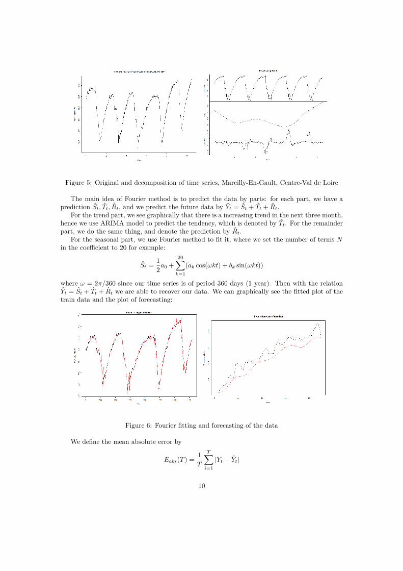
Figure 5: Original and decomposition of time series, Marcilly-En-Gault, Centre-Val de Loire
The main idea of Fourier method is to predict the data by parts: for each part, we have aprediction St, Tt, Rt, and we predict the future data by Yt = St + Tt + Rt.
For the trend part, we see graphically that there is a increasing trend in the next three month,hence we use ARIMA model to predict the tendency, which is denoted by Tt. For the remainderpart, we do the same thing, and denote the prediction by Rt.
For the seasonal part, we use Fourier method to fit it, where we set the number of terms Nin the coefficient to 20 for example:
St = 12a0 +
20∑k=1
(ak cos(ωkt) + bk sin(ωkt))
where ω = 2π/360 since our time series is of period 360 days (1 year). Then with the relationYt = St + Tt + Rt we are able to recover our data. We can graphically see the fitted plot of thetrain data and the plot of forecasting:
Figure 6: Fourier fitting and forecasting of the data
We define the mean absolute error by
Eabs(T ) = 1T
T∑i=1|Yt − Yt|
10

where T = 90 in our test data. We get the mean absolute error of Fourier method of water wellMarcilly-En-Gault is 0.08663402. As we can see, the Fourier predictor draws the brief outline ofour test data but there’s still a gap between the real data and the prediction. That’s because weuse ARIMA model to predict the trend part and the remainder part while the remainder part isdifficult to predict accurately with a simple autoarima process.
3.2 Random ForestThe second method we will use is Random forest, and we apply a fast implementation of randomforest ranger function in R to fit the data. We consider the following related factors:
Yt ∼ Yt + Pt + Jt +Mt +At
where Yt denotes the time series of last year’s level of underground water, Pt denotes the timeseries of last year’s precipitations, Jt,Mt, At denote date, month and year. We draw the fittingplot and the forecast plot:
Figure 7: Ranger fitting and forecasting of the data
The mean absolute error of Random Forest method of poin d’eau Marcilly-En-Gault is0.063399. We choose these factors because we think, a priori, that the level of groundwateris determined by the time flows and the weather conditions. While we don’t choose the currentprecipitation to train our model because we assume that our data is seasonal by year, so thatthe last year’s precipitation will be more helpful for us to do the analysis. Therefore, in order toexplore the seasonality of the time series, we choose the last year’s data. The result shows that itpredict better than Fourier, this means that the choice of factors in our model is very successful.
3.3 GAMNow we try GAM (Generalized Additive Model). The GAM can be formally written as
yi = β0 + f1(xi1) + · · ·+ fp(xip) + εi
where i = 1, · · ·N , yi follow some exponential family distribution, g is a link function (identical,logarithmic or inverse), y is a response variable, x1, · · · , xp are independent variables, β0 is anintercept, f1, · · · , fp are unknown smooth functions and ε is an i.i.d. random error.
11

The smooth function f is composed by sum of basis functions b and their correspondingregression coefficients β, which can be formally written as
f(x) =q∑
i=1bi(x) + βi
where q is basis dimension. Therefore, the model can be written in a linear way like
g(E(y)) = βX + ε
where X is a model matrix and β is a vector of regression coefficients.For our forecasting, we emphasize that interactions are a very important part of the regression
model, while with GAMs there are four main possibilities: x1 × x2, f(x1) × x2, f(x1) × f(x2)and f(x1) ⊗ f(x2). The fourth one is called tensor product interactions, which can be done byte function in R. There are many possibility of combinations that we could try, in our real data,we use three possible interactions of Yt, Pt, Mt and At, that we defined earlier in Random Forestmodel, to predict the future data:
GAM1: Yt ∼ f(Yt) + f(Pt) + f(Mt)⊗ f(At)
GAM2: Yt ∼ f(Yt)× f(Pt) + f(Mt)⊗ f(At)
GAM3: Yt ∼ f(Yt)⊗ f(Pt) + f(Mt)⊗ f(At)
Since the month and year are obviously not independent, and the same for undergroundwater level and precipitations because they are both effected by the weather condition, it’svery necessary to consider the product interaction and the tensor product interaction (terms off(x1, x2)). There are many possible combinations of these interactions, in the following picturewe will only show one possibility (GAM3), and later we will use expert aggregation to gatherthese model together and train a better one.
We draw the fitting plot and the forecast plot (for GAM3):
Figure 8: GAM fitting and forecasting of the data
The mean absolute error of GAM of poin d’eau Marcilly-En-Gault is 0.1418075. We see thatthis model performs not much better than Fourier and Ranger, this means that maybe the choiceof interactions in our GAM model is not very proper.
12

3.4 ComparisonNow we can apply several different models on all the 48 places that we have selected and usecross validation method to calculate the mean absolute error of each method on each place. Forthe cross validation procedure, we do as follows: suppose our train data varies from year 1 toN , we construct N − 1 subset of train data that vary from year N − 1 to N , from year N − 2to N , and finally from year 1 to N (the whole train data). We train our model on each subsetand apply it on the test data, for each subset of train data we get a mean absolute error, thenwe calculate the mean and get the final cross validation mean absolute error.
We predict original level, normalized day level, normalized week level, daily variation andweekly variation (which will be defined in the next section) based on the models we introduced,and we choose some remarkable point d’eau to compare the results, as shown in the followingtables.
Table 1: Comparison of models, original levelFourier Random Forest GAM3
Vizille 0.04784957 0.07746358 0.037255031Contres 0.11161227 0.57345545 0.04553232Sainte-Anne 0.017512226 0.073383598 0.008793767Marcilly-En-Gault 0.21834851 0.37985995 0.067675616
Table 2: Comparison of models, normalized day levelFourier Random Forest GAM3
Vizille 0.045102854 0.148652907 0.059233046Contres 0.008920658 0.101272965 0.005897183Sainte-Anne 0.017512226 0.073383598 0.015904798Marcilly-En-Gault 0.025868904 0.07704011 0.00629492
Table 3: Comparison of models, normalized week levelFourier Random Forest GAM3
Vizille 0.045063023 0.12841528 0.086638762Contres 0.009473171 0.090776812 0.012852736Sainte-Anne 0.01616033 0.214064289 0.05677534Marcilly-En-Gault 0.028282732 0.080346376 0.018294002
Table 4: Comparison of models, daily variationRandom Forest GAM3
Vizille 0.017440761 0.012411115Contres 0.042157904 0.044760385Sainte-Anne 0.43201123 0.081746667Marcilly-En-Gault 0.270276004 0.072867327
13

Table 5: Comparison of models, weekly variationRandom Forest GAM3
Vizille 0.023769802 0.025419212Contres 0.10186368 0.142490881Sainte-Anne 0.139291564 0.567256951Marcilly-En-Gault 0.180104143 0.151749724
We can see from these table that the performance of the three models really depend on thetime series we choose. For some series, for example, the daily variation in Sainte-Anne, maybethe seasonality is not obvious and hence the Fourier method performs very bad while the GAMmodel performs relatively well. But for those who are quite regular and easy to capture itsseasonality, Fourier will be a good model of prediction.
Therefore, building one model for each series can be appealing at a first sight because .However it is costly (how to manually study each series in order to catch the discontinuity pointsand train and evaluate the best suited model). Moreover, as we stated in introduction, it wouldwasteful to not look at interactions between wells and the huge amount of information broughtby past behavior of different wells. The second part of our study, Section 4, deals with thisaspect and tries to suggest a global model building on the behavior of all wells at hand.
4 An attempt at global modelling for ground water fluc-tuations
In this section, we investigate the performance of models that use past information of each wellsbehaviors to make prediction for a given well.
Yit is relative depth of well i at time t, for all (i, t) ∈ [N ]× [T ] measured in meters. We lookat :
• Daily variations : Yi,t+1−Yi,t
Yi,t
• One week overall variation : Yi,t+7−Yi,t
Yi,t
• Next week normalized level : Yi,t+7−mint∈T Yit
maxt∈T Yit−mint∈T Yit.
4.1 MethodologyData and models We consider the stationary data that passed Phillips-Perron test of sta-tionarity, so that N = 48. The time period is carefully chosen so that we have both recent andlarge data (there is a trade-off as shown in Section 2). We choose to consider daily data fromyears 2009 to 2017 which makes a total of T = 3287 days. We use the wide range of variablesdescribed earlier in Table 8 that we combine to make different model specifications (see Table 9).These variables are mostly built from meteorological data and past realizations and aim at an-ticipating variations of the water level by looking both at climate and geological conditions anddeviations form past trends. Note that, in this section, we do not make use models that need thebreaking points to be known such as GAM models or splines but rather concentrate on classicalmachine learning methods that learn patterns in an automated way alternatively for each well(GradientBoosting, CART, Random Forest).
14

Evaluation We consider different classes of models suited to this prevision problem and per-form model selection by retaining the model with the lowest cross-validated error metric. Giventhe fact that we work with differentiated data and for better interpretation we consider theMAD3 metric but also the RMSE (the metric used in the optimization process of most of thealgorithms used hereafter) in order to compare the models :
MAD = 1N
N∑i=1|yi − yi| , RMSE =
√√√√ 1N
N∑i=1
(yi − yi)2
The cross-validation procedure is the following : for i in [1, . . . , N ], train the model on individualsN−{i} for data such that x−2 < year < x and test it on the individual i for year = x. For eachindividual, repeat the inner-loop for x in [2012, 2013, 2014, 2015, 2016, 2017]. For each model, wereport the cross-validation error and if necessary, the hyper-parameters that have been used andoptimized on a separate CV loop using Gridsearch techniques.
4.2 Results from the training and optimization step (daily variations)To evaluate our models and covariate predicting power we proceed as follow : the linear modelserves as a baseline as such as models where only past realization is included (specification 1.).We compare then the results obtained in term of RMSE once other covariates are added to themodels (spec. 2., 22., 3. and 33.) and/or more involved models are used.
Day variation. Table 6 presents the results. Mean variation from one day to the otherare really low on average but quite volatile (µ = −0.011 and σ = 8.99) and very less correlated(ρ = 0.03) so that the different error scores obtained in specification (1.) which seem already highat a first sight are explained by these arguments. A further look at the minimum and maximumvalues of the error rate reveals however that some series are getting very high error rates andare prone to bias the result. We can deduce that some series are highly predictable while others(which are the ones with the highest number of peaks) exhibit high deviations from the modelprediction. Another interesting pattern is that the inclusion of meteorological variables does notseem to improve the CV MAD score (spe. 2. & 3.). Conversely, these variables explain wellthe variations given that when we do not include past realized values (spe. 22., 33.), the errorscore does not skyrocket. Again, this is due to low serial correlation in the variation rate of theprofondeur relative and mean that meteorological data does at least as best than predicting fromthe past realization. This gives insights on the fact that our variables must have a predictingpower but that the linear model is probably not suited to the problem or that all this measure-ments result in noise for this particular prediction task (see spe. 3). Daily variation is a verylocal phenomenon. We expect these variable to play more role at predicting week variation orweek normalized levels.
A CART algorithm is not very satisfactory on this dataset because it yields always to a depthof 1 when cross-validating which is of poor interest to model a complex phenomenon. Boostingtechniques, such as GBM (Adaboost), yield better results than the standard linear regressionmodel but which are not very sensitive to the addition of our meteorological data.
An interesting result lies in the prediction from a Random Forest algorithm. It is clear fromthe minimum error rates that, unlike the linear regression which remains an unflexible parametricform (Yit = α+ β′Xit + εit), the random forest made of 600 different trees with spe. 2 has been
3"Mean Absolute Deviation", more suited to deal with decimal values.
15

Table 6: Daily variations - main models’ resultsThe predicted variable unit is raw variation as defined earlier (Y = 0.02 means +2%). A Mean Absolute Deviation(MAD) of 1 means that on average if the model predicts no variation, the latent variable can be multiplied by a factor2. So such a result is a pretty bad result. The figures reported are the cross-validation error of the models with givenoptimized parameters trained and tested alternatively on the N − 1 wells and periods between (2012-2017). The columnTEST indicates the mean error across wells of the final model trained on all the data set and tested on the period(2018-2019). It is mechanically lower since it involved slightly less wells (36) and periods (about 1 year of data).
MAD RMSE TESTModel Spec. Mean Min. Max. Mean Min. Max.Linear model 1. 0.371 0.036 5.74 1.55 0.198 40.36 0.182
2. 0.401 0.090 5.74 1.57 0.239 40.36 0.23122. 0.390 0.077 5.73 1.48 0.103 40.36 0.2293. 0.408 0.100 5.74 1.58 0.247 40.36 0.25033. 0.398 0.087 5.73 1.49 0.116 40.36 0.249
CART (depth=1) 1. 0.369 0.029 5.74 . 0.198 40.36 0.18CART (depth=1) 2. 0.369 0.029 5.74 . 0.198 40.36 0.18CART (depth=1) 22. 0.369 0.029 5.74 . 0.198 40.36 0.18CART (depth=1) 3. 0.369 0.029 5.74 . 0.198 40.36 0.18CART (depth=1) 33. 0.369 0.029 5.74 . 0.198 40.36 0.18
GBM (sk=0.0001, ntree=50) 1. 0.356 0.014 5.73 . . . 0.176GBM (sk=0.0001, ntree=400) 2. 0.356 0.014 5.73 . . . 0.176
Random Forest (ntrees = 500) 1. 0.385 0.004 5.69 1.61 0.005 40.26 0.26(ntrees = 600) 2. 0.345 0.019 5.67 1.45 0.033 40.28 0.23(ntrees = 500) 22. 0.377 0.026 5.74 1.52 0.052 40.41 0.25(ntrees = 600) 3. 0.367 0.019 5.56 1.50 0.050 40.28 0.40(ntrees = 600) 33. 0.429 0.029 5.75 1.58 0.081 40.41 0.51
16
able to detect strong correlation and partition the feature space much more efficiently, at leastfor some series, and reaches the best cross-validated error rate on our train data set.
In a specification where we do not use the current values, minimum prediction errors are onlyof . This result suggest that this algorithm should be retained for the final prediction, but notusing it for each well.
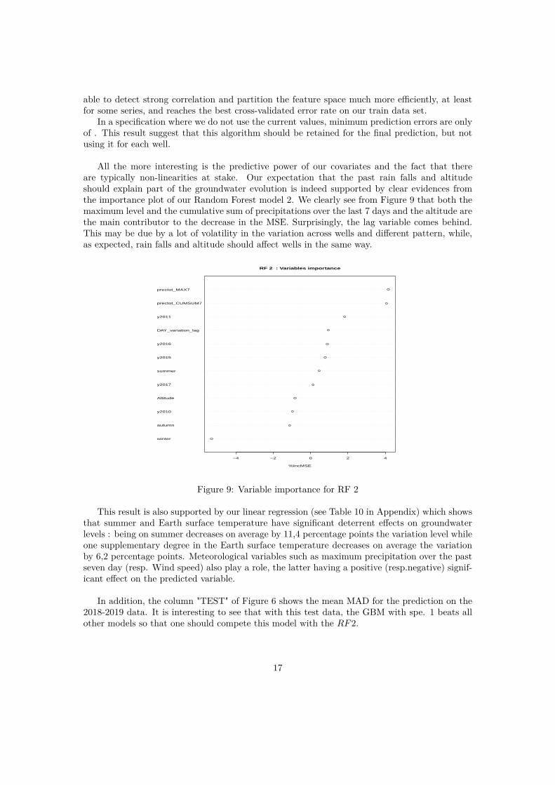
All the more interesting is the predictive power of our covariates and the fact that thereare typically non-linearities at stake. Our expectation that the past rain falls and altitudeshould explain part of the groundwater evolution is indeed supported by clear evidences fromthe importance plot of our Random Forest model 2. We clearly see from Figure 9 that both themaximum level and the cumulative sum of precipitations over the last 7 days and the altitude arethe main contributor to the decrease in the MSE. Surprisingly, the lag variable comes behind.This may be due by a lot of volatility in the variation across wells and different pattern, while,as expected, rain falls and altitude should affect wells in the same way.
winter
autumn
y2010
Altitude
y2017
summer
y2015
y2016
DAY_variation_lag
y2011
prectot_CUMSUM7
prectot_MAX7
−4 −2 0 2 4
RF 2 : Variables importance
%IncMSE
Figure 9: Variable importance for RF 2
This result is also supported by our linear regression (see Table 10 in Appendix) which showsthat summer and Earth surface temperature have significant deterrent effects on groundwaterlevels : being on summer decreases on average by 11,4 percentage points the variation level whileone supplementary degree in the Earth surface temperature decreases on average the variationby 6,2 percentage points. Meteorological variables such as maximum precipitation over the pastseven day (resp. Wind speed) also play a role, the latter having a positive (resp.negative) signif-icant effect on the predicted variable.
In addition, the column "TEST" of Figure 6 shows the mean MAD for the prediction on the2018-2019 data. It is interesting to see that with this test data, the GBM with spe. 1 beats allother models so that one should compete this model with the RF2.
17

4.3 Performances on new dataA deepest exploration of prediction results for our testing data shows the following results for theeasier, harder and median series (taken as the min, max and closer to the mean of the averageperformances across predictors) in Figure 10 :
0.00
0.05
0.10
Days
Ove
rnig
ht v
aria
tion
2018 2019
y RF 1 RF 2 RF 3 LM 1 LM 2
Predictions for the series with mininum test errors
0.0
0.5
1.0
Days
Ove
rnig
ht v
aria
tion
2018 2019
y RF 1 RF 2 RF 3 LM 1 LM 2
Predictions for a median series
−10
−5
05
1015
Days
Ove
rnig
ht v
aria
tion
2018 2019
y RF 1 RF 2 RF 3 LM 1 LM 2
Predictions for the series with highest test errors
Figure 10: "Easy", "Intermediate" and "Hard" series
There are three main take away from these graphs :
• Looking at figure 10, one can see that even for the "easier" series to predict, very smalldeviations are very hard to predict from our data and that the good performances (lowestaverage MAD error across all predictors) are in fact due to very weak variations of the seriesin general (see the scale of the y−axis). Nevertheless, some predictors do better than others: while our linear models are not able to capture any relevant pattern, one of our Random
18

Forest, RF2, fits rather accurately the fluctuations of the series. RF1 corresponds to aforest where only the lag realization is included. We can see from the graph that includingsome of our other covariates such as in RF2 tampers the wrong predicted peaks of RF1and lead to a better model. This result could be expected from the performances obtainedin the training and evaluating step.
• For what we call a "hard" series (bottom), we observe a similar symmetric pattern thatis, some models perform well at predicting deviations that are sometimes significantly farfrom zeros but high errors are here due to huge unexpected variations. We think that thesevariations could be punctual decisions or new events that our model is not able to detectfrom meteorological data or past behavior the series (exceptional events that are orthogonalto our predictors). Interestingly, the naive RF1 models is once again very volatile so thatone should prefer RF2 or RF3 (the main difference between the two being their ability tofit peaks and their predictions magnitude).
• Finally, the median case (top-right) is maybe the more interesting plot to look at. Here,the deviations from zero are of moderated size as expected and we see that, in line withour regression results, a simple linear model (AR) augmented with our climate variablesalready achieve to capture some variability of the series. LM3 is not included becauseit yields to spurious predictions which may be due to the curse of dimensionnality andomitted variables bias. It is worth to notice that again, one should prefer a parsimoniousmodel since RF3 and RF1 are much less precise than RF2.
These results are thus in line with the ones obtained in the training and evaluating step ofprevious Section 4.2. Particularly, they tell us that when looking at a global model for many se-ries, including only individual-specific variables such as lag and trends is not sufficient to capturenon-linearities and peculiarities for each series. At the opposite, when the number of individualis limited (recall that we switch from 4000 to 48), including too much variables can lead tooverfitting and erratic predictions. The model which lead to best predictions is the parsimoniousone that include both specific variables and common variables (such as rain, meteorological data,altitude etc.).
4.4 Results for next week normalized level and weekly variationsWe try in this section to give some results for other variables to predict (next week normalizedlevel and weekly variation). Due to time shortage, we do not provide an extended analysis suchas for daily variation. Nevertheless we have the following results :
1) It is much harder to make prediction at a week interval of time for level variation. Thebest aggregated linear model for the easiest series obtains a CV MAD score of 0.5 : onaverage, we miss the variation by 50 percentages point which is much bigger than what wepreviously obtained for daily variations. High errors are likely to be due to fast unantici-pated variations and so the length of these variation is mechanically higher than from oneday to another.
2) Past realization of the predicted variable explain well future evolution in case of normalizedlevels to be predicted. In fact, conversely to evolution rates, water levels are stronglycorrelated over time.
3) The best model for next week water level seems to include
19

Some cross-validated errors for these targets on which are based these results are available inthe following tables : Tables 11 and Table 12 (in Appendix). They are to be further completedbut already show basically that those prediction tasks are significantly "harder" to deal with.
5 Expert aggregationNow we do a naive try on expert aggregation, the main idea is due to Pierre Gaillard and theR package opera. Remember in section 3 that we have already trained one random forest modeland three GAM, now we will gather the four models together and do expert aggregation. Firstlet’s look at the oracle of these models:
Figure 11: Loss of the models
Then we initialize the algorithm by defining the type of algorithm (Ridge regression, expo-nentially weighted average forecaster, etc.), the possible parameters, and the evaluation criterion.Here we define the ML-Poly algorithm, which is evaluated by square loss. Now we perform on-line predictions using the predict method. At each time, step the aggregation rule form a newprediction and update the procedure. Here is the result:
20

Figure 12: Online aggregation
And we plot the prediction after online aggregation:
Figure 13: Expert prediction
The mean absolute error of expert prediction is 0.06365038, we see that it performs relativelywell as we expected.
21

6 Discussion of results and conclusionThe goal of this project was to answer the following questions : Can we predict groundwaterfluctuations using only public available data ? If yes, which modelling choices are performingbetter ? Does including information from other wells behaviors matter when predicting for agiven well ? After having dealt with the aggregation problem we wanted to answer the followingquestions : for which series do the aggregate predictor is better than the individual ones ? Forwhich series are they similar ? Finally we wondered whether drawing from convex combinationof our predictors, both at the individual and aggregate level would lead to better prediction suchas it could be the case by naively compute mean of predictions or use more involved methodssuch as EWA aggregation of expert.
Finally, our report suggests the following key results :
• Best models for individual predictions on some series are : Fourier method (for those whohave a good seasonality) and Random Forest (for some general series), anyway, for eachtime series we can apply expert aggregation and do a better prediction.
• Rain falls, altitude, Earth surface temperature, Wind and lag variables are the best pre-dicting features at the aggregated level.
• Parsimonious specifications should be preferred including mostly lag indicators of rainfallsand Temperature of the Earth Surface (as revealed by our linear regression).
• The global models achieving the best cross-validated and testing performances are ensembleand Boosted methods such as GBM and Random Forest.
• Predicting week normalized level of groundwater is more difficult than forecasting overnightvariation within a global model.Further research should finish the covering of other measures of fluctuations and look formore predicting variables in order to improve models accuracy and the global understandingof groundwater fluctuations.
22

ReferencesAbiyea, T., Masindia, K., Mengistub, H., and Demliec, M. (2018). Understanding thegroundwater-level fluctuations for better management of groundwater resource: A case inthe johannesburg region. Groundwater for Sustainable Development, 7:1–7.
Newey, W. K. and West, K. D. (1987). A simple, positive semi-definite, heteroskedasticity andautocorrelation consistent covariance matrix. Econometrica, 55(3):703–708.
Perron, P. (1988). Trends and random walks in macroeconomic time series. Journal of EconomicDynamics and Control, 12:297–332.
Shamsuddin, M. K. N., Kusin, F. M., Sulaiman, W. N. A., Ramli, M. F., Baharuddin, M. F. T.,and Adnan, M. S. (2017). Forecasting of groundwater level using artificial neural networkby incorporating river recharge and river bank infiltration. MATEC Web of Conferences,103:04007.
Shiri, J., Kisi, O., Yoon, H., Lee, K.-K., and Nazemi, A. H. (2013). Predicting groundwaterlevel of fluctuations with meteorological effect implications â a comparative study among softcomputing techniques. Computers & Geosciences, 56:32–44.
Sujay Raghavendra, N. and Deka, P. C. (2015). Forecasting monthly groundwater level fluc-tuations in coastal aquifers using hybrid wavelet packetâsupport vector regression. CogentEngineering, 2(1).
Van Asch, T. W. J. and Buma, J. T. (1997). Modelling groundwater fluctuations and thefrequency of movements of a landslidein the terres noires region of barcelonnette (france).Earth Surface Processes and Landforms, 22:131–141.
Vetrivel, N. and Elangovan, K. (2016). Prediction and forecasting of groundwater level fluctuationby ann technique. International Journal of Civil Engineering and Technology, 7:401–408.
Zare, M. and Koch, M. (2018). Groundwater level fluctuations simulation and prediction byanfis- and hybrid wavelet-anfis/fuzzy c-means (fcm) clustering models: Application to themiandarband plain. Journal of Hydro-environment Research, 8:63–76.
23

Appendix
Table 7: Distribution of selected water wells across regionRegion Cnt.Nouvelle Aquitaine 20Normandie 2Auvergne 5Bretagne 4Centre Val de Loire 4PACA 3Occitanie 3Mayotte 1Pays de la Loire 1Martinique 1La Reunion 1Ile de France 1Haut de France 1Guyanne 1Guadeloupe 1Grand-Est 1Bourgogne Franche-Comte 0Corse 1
24

Figure 14: Dates distributionDistribution of first year of data
First year of data available
Nb.
of w
ells
1900 1920 1940 1960 1980 2000 2020
050
100
150
Distribution of last year of data
Last year of data available
Nb.
of w
ells
1900 1920 1940 1960 1980 2000 2020
050
010
0015
0020
0025
00
Distribution of available period for each well
Number of years available
Nb.
of w
ells
0 20 40 60 80 100 120
050
100
150
25

Table 8: Main covariatesType Variable Label UnitTrend
Summer, autumn, winter Dummies for seasons 0/1yx, mx Dummies for years and months 0/1t TimeY_lag Lag predicted variable raw var/norm. lvl
Altitude Well’s altitude m
MeteoPRECTOT Precipitations mmPS Surface Pressure kPaQV2M Specific Humidity at 2 Meters kgRH2M Relative Humidity at 2 Meters %T10M_MAX Maximum Temperature at 10 Meters C◦T10M_MIN Minimum Temperature at 10 Meters C◦T2M_MAX Maximum Temperature at 2 Meters C◦T2M_MIN Minimum Temperature at 2 Meters C◦TS_MAX Maximum Earth Skin Temperatur C◦TS_MIN Minimum Earth Skin Temperature C◦WS2M_MAX Maximum Wind Speed at 2 Meters m/sWS2M_MIN Minimum Wind Speed at 2 Meters m/sWS50M Wind Speed at 50 Meters m/s
Combinationsx_CUMSUM7 Cumulative sum over last 7 daysx_CUMSUM31 Cumulative sum over the last 31 daysx_MEAN7 Mean over the last 7 daysx_MEAN31 Mean over the last 31 days
26

Table 9: Model specificationsSpecification Variables included in the model1. DAY_variation_lag
2. DAY_variation_lag + summer + autumn + winter + y2010 + y2011 + y2015 + y2016+ y2017 + PRECTOT_CUMSUM7 + PRECTOT_MAX7 + Altitude
22. summer + autumn + winter + y2010 + y2011 + y2015 + y2016 + y2017+ PRECTOT_CUMSUM7 + prectot_MAX7 + Altitude
3. DAY_variation_lag + summer + autumn + winter + y2010 + y2011 + y2015 + y2016+ y2017 + PRECTOT_CUMSUM7 + PRECTOT_MAX7 + PRECTOT_CUMSUM31QV2M_MEAN7 + T2M_MAX_MEAN7 + RH2M_MEAN7 + T2M_MIN_MEAN7+ WS2M_MIN_MEAN7 + T10M_MAX_MEAN7 + TS_MAX_MEAN7+ WS50M_MEAN7 + PS_MEAN7 + PS_MEAN31 + T10M_MIN_MEAN7+ TS_MIN_MEAN7
33. summer + autumn + winter + y2010 + y2011 + y2015 + y2016+ y2017 + PRECTOT_CUMSUM7 + PRECTOT_MAX7 + PRECTOT_CUMSUM31QV2M_MEAN7 + T2M_MAX_MEAN7 + RH2M_MEAN7 + T2M_MIN_MEAN7+ WS2M_MIN_MEAN7 + T10M_MAX_MEAN7 + TS_MAX_MEAN7+ WS50M_MEAN7 + PS_MEAN7 + PS_MEAN31 + T10M_MIN_MEAN7+ TS_MIN_MEAN7
4. WEEK_level_lag
44. WEEK_level_lag + normalized_Y_mean7days + normalized_Y_mean2daysdev_Y_lastyear + summer + autumn + winter + PRECTOT_CUMSUM7PRECTOT_CUMSUM31 + PRECTOT_MAX7 + Altitude
5. normalized_Y_mean7days + normalized_Y_mean2days + dev_Y_lastyear+ summer + autumn + winter + prectot_CUMSUM7+ PRECTOT_CUMSUM31 +PRECTOT_MAX7 + Altitude)
6. WEEK_level_lag + normalized_Y_mean7days + normalized_Y_mean2days +normalized_Y_last_year + dev_Y_lastyear + summer + autumn + winter +Altitude + PRECTOT_CUMSUM7 + PRECTOT_CUMSUM31 + PRECTOT_MAX7 + Altitude+ y2010 + y2011 + y2015 + y2016 + y2017 + PS_MEAN7 + PS_MEAN31 + QV2M_MEAN7+ RH2M_MEAN7 + T10M_MAX_MEAN7 + T10M_MIN_MEAN7 + T2M_MAX_MEAN7+ T2M_MIN_MEAN7 + TS_MAX_MEAN7 + TS_MIN_MEAN7 + WS50M_MEAN7 +WS2M_MIN_MEAN7
66. WEEK_level_lag + normalized_Y_mean7days + normalized_Y_mean2days +normalized_Y_last_year + dev_Y_lastyear + summer + autumn + winter + Altitude+ PRECTOT_CUMSUM7 + PRECTOT_CUMSUM31 + PRECTOT_MAX7 + Altitude + y2010+ y2011 + y2015 + y2016 + y2017 + PS_MEAN7 + PS_MEAN31 + QV2M_MEAN7 +RH2M_MEAN7 + T10M_MAX_MEAN7 + T10M_MIN_MEAN7 + T2M_MAX_MEAN7 +T2M_MIN_MEAN7 + TS_MAX_MEAN7 + TS_MIN_MEAN7 + WS50M_MEAN7 +WS2M_MIN_MEAN7
7. WEEK_level_lag
8. WEEK_level_lag + normalized_Y_mean7days + normalized_Y_mean2daysdev_Y_lastyear + summer + autumn + winter + PRECTOT_CUMSUM7PRECTOT_CUMSUM31 + PRECTOT_MAX7 + Altitude
88. normalized_Y_mean7days + normalized_Y_mean2days + dev_Y_lastyear+ summer + autumn + winter + prectot_CUMSUM7+ PRECTOT_CUMSUM31 +PRECTOT_MAX7 + Altitude)
9. WEEK_level_lag + normalized_Y_mean7days + normalized_Y_mean2days +normalized_Y_last_year + dev_Y_lastyear + summer + autumn + winter +Altitude + PRECTOT_CUMSUM7 + PRECTOT_CUMSUM31 + PRECTOT_MAX7 + Altitude+ y2010 + y2011 + y2015 + y2016 + y2017 + PSM EAN7 + P S_MEAN31 +QV2M_MEAN7 + RH2M_MEAN7 + T10M_MAX_MEAN7 + T10M_MIN_MEAN7 +T2M_MAX_MEAN7 + T2M_MIN_MEAN7 + TS_MAX_MEAN7 + TS_MIN_MEAN7 +WS50M_MEAN7 + WS2M_MIN_MEAN7
99. WEEK_level_lag + normalized_Y_mean7days + normalized_Y_mean2days+ normalized_Y_last_year + dev_Y_lastyear + summer + autumn + winter +Altitude + PRECTOT_CUMSUM7 + PRECTOT_CUMSUM31 + PRECTOT_MAX7 + Altitude +y2010 + y2011 + y2015 + y2016 + y2017 + PSM EAN7 + P S_MEAN31+ QV2M_MEAN7 + RH2M_MEAN7 + T10M_MAX_MEAN7 + T10M_MIN_MEAN7 +T2M_MAX_MEAN7 + T2M_MIN_MEAN7 + TS_MAX_MEAN7 + TS_MIN_MEAN7 +WS50M_MEAN7 + WS2M_MIN_MEAN7
The double digit specifications indicate that the lagged predicted variable is not included to the model.
27

Table 10: Results from linear regressions (Daily variation)Dependent variable:DAY_variation
(1) (2) (3) (4) (5)
DAY_variation_lag 0.033∗∗∗ 0.032∗∗∗ 0.032∗∗∗(0.003) (0.003) (0.003)
summer -0.114∗ -0.118∗ -0.091 -0.094(0.066) (0.066) (0.084) (0.084)
autumn 0.043 0.044 0.022 0.023(0.067) (0.067) (0.072) (0.072)
winter 0.036 0.037 -0.046 -0.047(0.067) (0.067) (0.079) (0.079)
y2010 -0.011 -0.011 -0.001 -0.001(0.079) (0.079) (0.080) (0.080)
y2011 -0.024 -0.025 -0.009 -0.009(0.079) (0.079) (0.080) (0.080)
y2015 -0.010 -0.011 -0.005 -0.005(0.079) (0.079) (0.079) (0.079)
y2016 -0.011 -0.011 -0.006 -0.006(0.079) (0.079) (0.079) (0.079)
y2017 -0.205∗∗∗ -0.212∗∗∗ -0.226∗∗∗ -0.233∗∗∗(0.079) (0.079) (0.086) (0.086)
prectot_CUMSUM7 0.0001 0.0001 0.0003 0.0003(0.0005) (0.0005) (0.001) (0.001)
prectot_MAX7 0.009∗∗∗ 0.010∗∗∗ 0.005 0.005(0.003) (0.003) (0.004) (0.004)
Altitude -0.00000 -0.00000(0.0001) (0.0001)
PRECTOT_CUMSUM31 -0.0003 -0.0003(0.0003) (0.0003)
QV2M_MEAN7 -0.490 -0.658(40.579) (40.600)
T2M_MAX_MEAN7 0.032 0.034(0.044) (0.044)
RH2M_MEAN7 -0.005 -0.005(0.007) (0.007)
T2M_MIN_MEAN7 0.050 0.051(0.166) (0.167)
WS2M_MIN_MEAN7 -0.108 -0.110(0.067) (0.067)
T10M_MAX_MEAN7 -0.0002 -0.0002(0.0003) (0.0003)
TS_MAX_MEAN7 -0.062∗ -0.064∗(0.035) (0.035)
WS50M_MEAN7 0.059∗ 0.060∗(0.034) (0.034)
PS_MEAN7 -0.004 -0.004(0.059) (0.059)
PS_MEAN31 -0.005 -0.006(0.060) (0.060)
T10M_MIN_MEAN7 -0.011 -0.011(0.124) (0.124)
TS_MIN_MEAN7 -0.005 -0.005(0.051) (0.051)
Constant -0.011 -0.050 -0.051 1.501 1.544(0.023) (0.061) (0.061) (0.962) (0.962)
Observations 147,717 146,367 146,367 146,367 146,367R2 0.001 0.001 0.0002 0.001 0.0003Adjusted R2 0.001 0.001 0.0001 0.001 0.0001Residual Std. Error 8.989 (df = 147715) 9.023 (df = 146354) 9.028 (df = 146355) 9.023 (df = 146342) 9.028 (df = 146343)F Statistic 156.885∗∗∗ (df = 1; 147715) 14.527∗∗∗ (df = 12; 146354) 2.366∗∗∗ (df = 11; 146355) 7.834∗∗∗ (df = 24; 146342) 1.762∗∗ (df = 23; 146343)
Note: ∗p<0.1; ∗∗p<0.05; ∗∗∗p<0.01
28

Table 11: Week variations - main models’ resultsThe predicted variable unit is raw variation as defined earlier (Y = 0.02 means +2%). A Mean Absolute Deviation(MAD) of 1 means that on average if the model predicts no variation, the latent variable can be multiplied by a factor2. So such a result is a pretty bad result. The figures reported are the cross-validation error of the models with givenoptimized parameters trained and tested alternatively on the N − 1 wells and periods between (2012-2017). The columnTEST indicates the mean error accross wells of the final model trained on all the data set and tested on the period(2018-2019). It is mechanically lower since it involved slightly less wells (36) and periods (about 1 year of data).
MAD RMSE TESTModel Spec. Mean Min. Max. Mean Min. Max.Linear model 7. 3.81 0.757 26.69 19.51 3.16 174.8 .
8. 3.91 0.922 26.71 19.52 3.18 174.8 .88. 3.55 0.54 26.53 17.89 0.72 173.4 .9. 3.93 0.95 26.71 19.53 3.20 174.8 .99. 3.91 0.93 26.70 19.52 3.18 174.8 .
GBM (sk=0.0001, ntree=50) 7. 3.29 0.10 26.49 17.61 0.13 173.3 .GBM (sk=0.0001, ntree=50) 8. 3.29 0.10 26.49 17.61 0.13 173.3 .
Random Forest (ntrees = 500) 7. . . . . . . .(ntrees = 600) 8. . . . . . . .(ntrees = 500) 88. . . . . . . .(ntrees = 600) 9. . . . . . . .(ntrees = 600) 99. . . . . . . .
Table 12: Next week normalized - main models’ resultsThe predicted variable unit is week normalized level as defined earlier (Y = 0.5 means that the level is at the centerof the segment (min, max)). A Mean Absolute Deviation (MAD) of 1 means that on average if the model predicts novariation, the latent variable can reach its maximum value. So such a result is a pretty bad result. The figures reportedare the cross-validation error of the models with given optimized parameters trained and tested alternatively on theN −1 wells and periods between (2012-2017). The column TEST indicates the mean error across wells of the final modeltrained on all the data set and tested on the period (2018-2019). It is mechanically lower since it involved slightly lesswells (36) and periods (about 1 year of data).
MAD RMSE TESTModel Spec. Mean Min. Max. Mean Min. Max.Linear model 4. 0.30 0.23 0.44 0.36 0.29 0.51 .
5. 0.29 0.23 0.44 0.35 0.28 0.50 .55. 0.30 0.23 0.44 0.36 0.29 0.51 .6. 0.30 0.23 0.44 0.36 0.29 0.51 .66. 0.29 0.23 0.44 0.35 0.28 0.50 .
GBM (sk=0.0001, ntree=50) 4. . . . . . . .GBM (sk=0.0001, ntree=50) 5. . . . . . . .
Random Forest (ntrees = 500) 4. . . . . . . .(ntrees = 600) 5. . . . . . . .(ntrees = 500) 55. . . . . . . .(ntrees = 600) 6. . . . . . . .(ntrees = 600) 66. . . . . . . .
29


