Data Mining with RLinear Classifiers and the Perceptron Algorithm

Hugh Murrell

references

These slides are based on a notes by Cosma Shalizi and anessay by Charles Elkan, but are self contained and access tothese documents is not essential.

for further background wikipedia is a useful source ofinformation.

assumptions

To introduce classifiers we will assume that ~x is a vector ofreal-valued numerical input features. There are p of them.

The variable we are trying to learn is called the response, Y .

Inititially we will assume that Y is a binary class and it willsimplify the book-keeping to say that the two classes are +1and −1.

In linear classification, we seek to divide the two classes by alinear separator in the feature space.

If p = 2 the separator is a line, if p = 3 it is a plane, and ingeneral it is a p − 1 dimensional hyperplane in a p dimensionalspace;

some geometry

We can specify the orientation of a plane by a vector ~w in thedirection perpendicular to it.

There are infinitely many parallel planes with the sameorientation.

We need to pick out one of them, which we can do by fixingits distance from the origin, b say.

R code to generate data separated by:

X2 = X1 +1

2

> x1 <- runif(30,-1,1)

> x2 <- runif(30,-1,1)

> x <- cbind(x1,x2)

> Y <- ifelse(x2>0.5+x1,+1,-1)

> plot(x,pch=ifelse(Y>0,"+","-"),

+ xlim=c(-1,1),ylim=c(-1,1),cex=2)

> abline(0.5,1)

> points(c(0,0),c(0,0),pch=19)

> lines(c(0,-0.25),c(0,0.25),lty=2)

> arrows(-0.3,0.2,-0.4,0.3)

> text(-0.45,0.35,"w",cex=2)

> text(-0.0,0.15,"b",cex=2)

data with linear separator

−

+

−−

+ −

+

−

+

+ −

−

−

−

−

−−

−

−

−

+

−

−

−

−−

−

+

−

−

−1.0 −0.5 0.0 0.5 1.0

−1.

0−

0.5

0.0

0.5

1.0

x1

x2

wb

Figure: Example of a linear separator: (+ and -) indicate points inthe positive and negative classes. The perpendicular vector ~w fixesthe orientation of the separator. The directed distance b from theorigin fixes the position of the separator.

using a separator to predict class

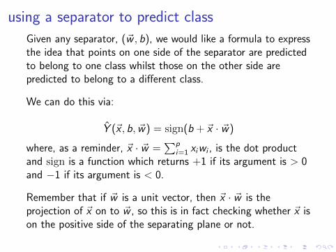
Given any separator, (~w , b), we would like a formula to expressthe idea that points on one side of the separator are predictedto belong to one class whilst those on the other side arepredicted to belong to a different class.

We can do this via:

Y (~x , b, ~w) = sign(b + ~x · ~w)

where, as a reminder, ~x · ~w =∑p

i=1 xiwi , is the dot productand sign is a function which returns +1 if its argument is > 0and −1 if its argument is < 0.

Remember that if ~w is a unit vector, then ~x · ~w is theprojection of ~x on to ~w , so this is in fact checking whether ~x ison the positive side of the separating plane or not.

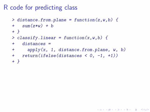
R code for predicting class

> distance.from.plane = function(z,w,b) {

+ sum(z*w) + b

+ }

> classify.linear = function(x,w,b) {

+ distances =

+ apply(x, 1, distance.from.plane, w, b)

+ return(ifelse(distances < 0, -1, +1))

+ }

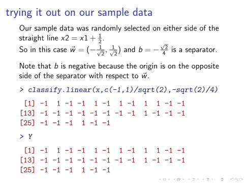
trying it out on our sample data

Our sample data was randomly selected on either side of thestraight line x2 = x1 + 1

2.

So in this case ~w = (− 1√2, 1√

2) and b = −

√24

is a separator.

Note that b is negative because the origin is on the oppositeside of the separator with respect to ~w .

> classify.linear(x,c(-1,1)/sqrt(2),-sqrt(2)/4)

[1] -1 1 -1 -1 1 -1 1 -1 1 1 -1 -1

[13] -1 -1 -1 -1 -1 -1 -1 -1 1 -1 -1 -1

[25] -1 -1 -1 1 -1 -1

> Y

[1] -1 1 -1 -1 1 -1 1 -1 1 1 -1 -1

[13] -1 -1 -1 -1 -1 -1 -1 -1 1 -1 -1 -1

[25] -1 -1 -1 1 -1 -1

the peceptron algorithm

In 1958 Frank Rosenblatt created much enthusiasm when hepublished a method called the perceptron algorithm that isguarateed to find a separator in a separable data set.

The basic algorithm is very simple, assuming the separatorpasses through the origin and that the training labels Yi areeither −1 or +1:

initialize ~w = 0while any training observation (~x ,Y ) is not classified correcty

set ~w = ~w + Y~x

Incorrectly classified training vectors are simply added to (orsubracted from) the separator normal, ~w .

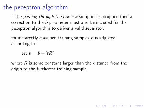
the peceptron algorithm

If the passing through the origin assumption is dropped then acorrection to the b parameter must also be included for thepeceptron algorithm to deliver a valid separator.

for incorrectly classified training samples b is adjustedaccording to:

set b = b + YR2

where R is some constant larger than the distance from theorigin to the furtherest training sample.

full peceptron code> euclidean.norm = function(x) {sqrt(sum(x * x))}

> perceptron = function(x, y, learning.rate=1) {

+ w = vector(length = ncol(x)) # initialize w

+ b = 0 # Initialize b

+ k = 0 # count updates

+ R = max(apply(x, 1, euclidean.norm))

+ made.mistake = TRUE # to enter the while loop

+ while (made.mistake) {

+ made.mistake=FALSE # hopefully

+ yc <- classify.linear(x,w,b)

+ for (i in 1:nrow(x)) {

+ if (y[i] != yc[i]) {

+ w <- w + learning.rate * y[i]*x[i,]

+ b <- b + learning.rate * y[i]*R^2

+ k <- k+1

+ made.mistake=TRUE

+ }

+ } }

+ s = euclidean.norm(w)

+ return(list(w=w/s,b=b/s,updates=k))

+ }

Note that because a separator (~w , b) classifies identically toany scaled counterpart (s~w , sb), we choose to scale theseparator so that the normal, ~w , is returned as a unit vector.

testing the peceptron code

> (p <- perceptron(x,Y))

$w

x1 x2

-0.7048230 0.7093832

$b

[1] -0.3229594

$updates

[1] 42

> y <- classify.linear(x,p$w,p$b)

> sum(abs(Y-y))

[1] 0

the separator returned by the peceptron

−

+

−−

+ −

+

−

+

+ −

−

−

−

−

−−

−

−

−

+

−

−

−

−−

−

+

−

−

−1.0 −0.5 0.0 0.5 1.0

−1.

0−

0.5

0.0

0.5

1.0

x1

x2

Figure: our separable data set with the original separator,X2 = X1 + 1

2 , shown in blue whilst the separator returned by thepeceptron is shown in red.

convergence of the peceptron algorithm

The perceptron algorithm is mathematically important becauseof a theorem about its convergence, due to Novikoff in 1962.

Assumptions: Let R = max ||~xt || and suppose that thelearning task is solvable via a separator that passes throughthe origin. i.e. there exists some vector ~w ∗ of unit length andsome δ > 0 such that Yt( ~w ∗ · ~xt) > δ for all t.

Theorem: Under these assumptions, the perceptron algorithmconverges after at most (R

δ)2 updates.

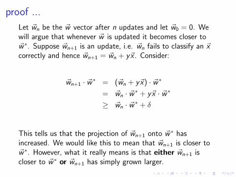
proof ...

Let ~wn be the ~w vector after n updates and let ~w0 = 0. Wewill argue that whenever ~w is updated it becomes closer to~w ∗. Suppose ~wn+1 is an update, i.e. ~wn fails to classify an ~xcorrectly and hence ~wn+1 = ~wn + y~x . Consider:

~wn+1 · ~w ∗ = (~wn + y~x) · ~w ∗

= ~wn · ~w ∗ + y~x · ~w ∗

≥ ~wn · ~w ∗ + δ

This tells us that the projection of ~wn+1 onto ~w ∗ hasincreased. We would like this to mean that ~wn+1 is closer to~w ∗. However, what it really means is that either ~wn+1 iscloser to ~w ∗ or ~wn+1 has simply grown larger.

proof continued ...

Consider the Euclidean length of ~wn+1:

||~wn+1||2 = ||~wn + y~x ||2

= ||~wn||2 + 2y(~wn · ~x) + ||~x ||2

≤ ||~wn||2 + R2 (since y(~wn · ~x) ≤ 0)

Thus, after N actual updates we know two facts:||~wN ||2 ≤ NR2 and ~wN · ~w ∗ ≥ Nδ. Putting these together:

Nδ ≤ ~wN · ~w ∗ ≤ ||~wN || ≤ R√N and so

√N ≤ R

δ

which means N is bounded and updates must cease eventually.

example data set

When the target variable has more than two classes theperceptron may still be used to generate a classification rule byrepeatedly separating on a one versus the rest basis.To demonstrate we will make use of the classic iris data setfrom R’s datasets collection.

> data(iris)

> dim(iris) # 150 measurements of 5 attributes

[1] 150 5

> names(iris)

[1] "Sepal.Length" "Sepal.Width"

[3] "Petal.Length" "Petal.Width"

[5] "Species"

target attribute: Species

The Species attribute in the iris dataset is categorical.

> summary(iris$Species)

setosa versicolor virginica

50 50 50

The remaining four iris attributes are real valued descriptors.Can we use these real valued attributes to predict iris species?First we consider all possible bi-variate scatter plots.

iris scatter plots

> data(iris)

> pairs(iris[,1:4], col=iris$Species)

Sepal.Length

2.0 3.0 4.0 0.5 1.5 2.5

4.5

5.5

6.5

7.5

2.0

3.0

4.0

Sepal.Width

Petal.Length

12

34

56

7

4.5 5.5 6.5 7.5

0.5

1.5

2.5

1 2 3 4 5 6 7

Petal.Width

Figure: all possible bivariate scatter plots for the iris dataset.

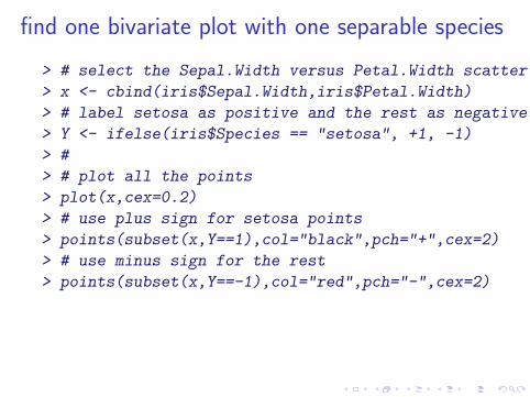
find one bivariate plot with one separable species

> # select the Sepal.Width versus Petal.Width scatter plot

> x <- cbind(iris$Sepal.Width,iris$Petal.Width)

> # label setosa as positive and the rest as negative

> Y <- ifelse(iris$Species == "setosa", +1, -1)

> #

> # plot all the points

> plot(x,cex=0.2)

> # use plus sign for setosa points

> points(subset(x,Y==1),col="black",pch="+",cex=2)

> # use minus sign for the rest

> points(subset(x,Y==-1),col="red",pch="-",cex=2)

setosa is separable

2.0 2.5 3.0 3.5 4.0

0.5

1.0

1.5

2.0

2.5

x[,1]

x[,2

]

++ ++ +++++ + ++++ +

+++ ++++

+++++++++

+++++ +++ +++ +

+++ ++ ++

−−−−

−−

−

−−−

−

−

−

−− −−

−

−

−

−

−−

−−−−−

−

−−−−

− − −−− −−−

−−

−− −−−

−−

−

−−

−

−−

− −−

−

−−−−

− −

−

−−

−

−−−

−−

−− −−

−− −−

−−

− −

−−−−−

−

−−

−

− −−

−

Figure: Scatter of Sepal.Width versus Petal.Width for setosaversus all other species

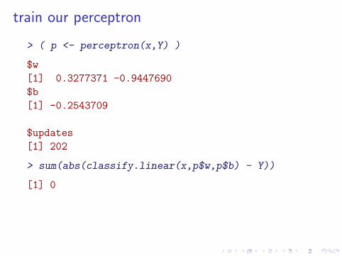
train our perceptron

> ( p <- perceptron(x,Y) )

$w

[1] 0.3277371 -0.9447690

$b

[1] -0.2543709

$updates

[1] 202

> sum(abs(classify.linear(x,p$w,p$b) - Y))

[1] 0

replot and view the separation boundary

> plot(x,cex=0.2)

> points(subset(x,Y==1),col="black",pch="+",cex=2)

> points(subset(x,Y==-1),col="red",pch="-",cex=2)

> # compute intercept on y axis of separator

> # from w and b

> intercept <- - p$b / p$w[[2]]

> # compute slope of separator from w

> slope <- - p$w[[1]] /p$ w[[2]]

> # draw separating boundary

> abline(intercept,slope,col="green")

separation boundary

2.0 2.5 3.0 3.5 4.0

0.5

1.0

1.5

2.0

2.5

x[,1]

x[,2

]

++ ++ +++++ + ++++ +

+++ ++++

+++++++++

+++++ +++ +++ +

+++ ++ ++

−−−−

−−

−

−−−

−

−

−

−− −−

−

−

−

−

−−

−−−−−

−

−−−−

− − −−− −−−

−−

−− −−−

−−

−

−−

−

−−

− −−

−

−−−−

− −

−

−−

−

−−−

−−

−− −−

−− −−

−−

− −

−−−−−

−

−−

−

− −−

−

Figure: Peceptron separation of setosa from all other species

non-separable data

We now have one rule via classify.linear(x,w,b) tocheck if an observation is of species setosa or not.

If it is not then we need one more rule to separateversicolor from virginica.

A study of the all pairs iris scatterplots should convince youthat no pair of attributes will deliver a linear separationboundary for versicolor from virginica.

It would be nice if the peceptron algorithm produced the bestpossible linear separating line in cases of non-separableobservations.

Unfortunately this does not happen because the peceptronenters an endless cycle of updates when perfect separation isnot possible.

exercises

I code: Create an R script for the peceptron codepresented in these slides. Your script should include thecode for the peceptron as well as testing code.

I prove: that the decision boundary generated by (~w , b) isidentical to the decision boundary generated by (s~w , sb)for any scaling parameter s.

I plot: add a peceptron.plot(x,y,w,b) function toyour R script that in the two dimensional case, generatesa scatter plot of the training data with a superimposedpeceptron decision boundary. Include code to test yourplot function.

I non-separable: add parameters and code to yourpeceptron algorithm that causes the peceptron toterminate after a user specified number of updates andthen returns the best decision boundary discovered so far.

exercises ...

I iris classification: use your enhanced peceptron tocomplete the iris classification problem outlined in theseslides by generating a second decision boundary similar tothe one shown on the next slide.

1 2 3 4 5 6 7

0.5

1.0

1.5

2.0

2.5

Petal.Length

Pet

al.W

idth

+

++

+

+ +

+ ++

+

++++

++

+

++

+

++ ++

++++

+

+++

+

+ +

++

+++++

+

++

+

+++

+

−−−−−−−−−−−−−−−

−−−−−−−

−−−−

−−−−−−−−−−−−−−−−−

−−−−−−−

−− −−

−−−

−−−

−

−

−

−− −−

−

−

−

−

−−

−−− −−

−

−−−−

−−−−−−− −−

−−

−−−−−−

Figure: Peceptron separation of virginica from all other species

Submit via e-mail a single R script that contains yourenhanced perceptron code, deals with the classificationproblem mentioned above and makes use of commentstatements to present your proof.

deadline: 6h00 on Monday the 25th of April.

Use: dm07-STUDENTNUMBER.R a as the filename for the script.

Use: dm07-STUDENTNUMBER as the subject line of your email.

There will be no extensions. No submission implies no mark.