PDHonline Course L155G (5 PDH) Data Models and Data processing in GIS PDH Online | PDH Center 5272 Meadow Estates Drive Fairfax, VA 22030-6658 Phone & Fax: 703-988-0088 www.PDHonline.org www.PDHcenter.com An Approved Continuing Education Provider 2012 Instructor: Steve Ramroop, Ph.D.
This lecture is the continuation of the GIS topic identified in the course description which is Data Models, Data Structure
and Data Management.
Slide 2
2L155 - GIS Data Models and Data Processing
Lecture 2Dr. Steve Ramroop
Spatial Data Models– Hierarchical data model– Network data model– Relational data model– Object oriented data model– Temporal data model
This is the contents of this lecture. Details into each of the data model are presented in this lecture. The structure of this
lecture is that each data model is presented with a description of its common characteristics. The first type of spatial data
model adopted when GIS was first introduced was the Hierarchical data model.
Slide 3
3L155 - GIS Data Models and Data Processing
Lecture 2Dr. Steve Ramroop
1) Hierarchical Data Model
data sets are organized in a hierarchical tree structurerelationships among the data sets entities are defined by the organization of the hierarchythat is the hierarchy is encoded in the records for each entity
This slide gives some characteristics of the Hierarchical Data Model. In this model the organization’s structure is explicitly
defined in the model. The hierarchy had to be encoded into the records of each entity presented on the map. The
following slide gives a graphic example.
Slide 4
4L155 - GIS Data Models and Data Processing
Lecture 2Dr. Steve Ramroop
> Courses are taught by Professors
> Students are in a DepartmentOrganization of a database using the Hierarchical Data Model
This slide shows and example of a hierarchical data model adopted in the context of University that has professors who
teach courses. As shown in the figure there is a relationship between University and Department; Department and
Students; Department and Professors; and Professors and courses.
In this model a “child” can have only one “parent”. That is, in this data model, lower levels of the hierarchy cannot have
multiple higher level relationships. For example “Courses” are taught by “Professors”, and “Students” are in a
“Department”.
Slide 5
5L155 - GIS Data Models and Data Processing
Lecture 2Dr. Steve Ramroop
Notes on the previous figure:– The highest level of the hierarchy is called the “root” which
consists of one entity– Except for the root, every element has one higher level
element related to it, that is called its “parent” and one or more subordinate elements is called the “children”
an element can have only one parent but can have multiple children
– All relations are many-to-one relation or one-to-one relatione.g. many departments belong to one university and many students
are in each department– Information is retrieved by traversing the hierarchy
structure starting from the root of the hierarchy
This slide gives some notes of the hierarchical data model. Note that in this model searches are done by traversing the
entire hierarchy starting from the root.
Slide 6
6L155 - GIS Data Models and Data Processing
Lecture 2Dr. Steve Ramroop
1
2 3
4 5
6
a2
a1
a3
a4
a5
a7
a6
1
a2a1 a3 a4a4 a5 a6 a7
4 1 2 2 3 3 4 3 4 4 5 5 6 3 6
AB
A B
MAP
An example:
This is another graphic representation of how the hierarchy data model is applied to a map representation.
The Map is the root, A and B are the sections of the Map. Each section is defined by a set of arcs labeled by a lower case
(a) with a sequential numbering as its subscript. An arc is defined by a start node and an end node. Nodes are labeled at
the intersection of arcs and the nodes are numbered sequentially starting from 1 and ending at 6. Notice that arc a4 is
repeated under sections A and B.
Slide 7
7L155 - GIS Data Models and Data Processing
Lecture 2Dr. Steve Ramroop
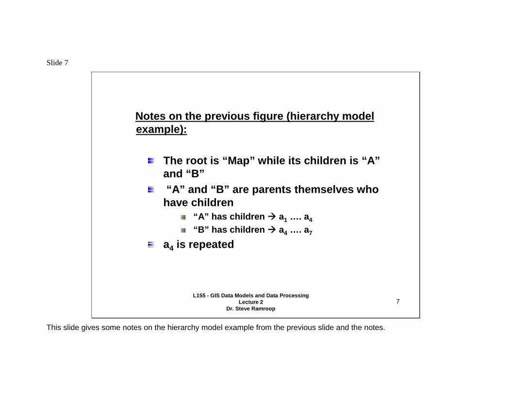
Notes on the previous figure (hierarchy model example):
The root is “Map” while its children is “A”and “B”“A” and “B” are parents themselves who
have children “A” has children a1 …. a4
“B” has children a4 …. a7
a4 is repeated
This slide gives some notes on the hierarchy model example from the previous slide and the notes.
Slide 8
8L155 - GIS Data Models and Data Processing
Lecture 2Dr. Steve Ramroop
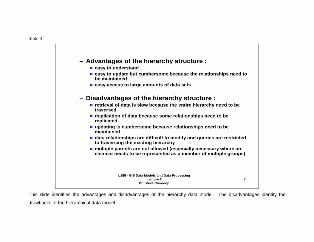
– Advantages of the hierarchy structure :easy to understandeasy to update but cumbersome because the relationships need to be maintainedeasy access to large amounts of data sets
– Disadvantages of the hierarchy structure :retrieval of data is slow because the entire hierarchy need to be traversedduplication of data because some relationships need to be replicatedupdating is cumbersome because relationships need to be maintaineddata relationships are difficult to modify and queries are restricted to traversing the existing hierarchymultiple parents are not allowed (especially necessary where an element needs to be represented as a member of multiple groups)
This slide identifies the advantages and disadvantages of the hierarchy data model. The disadvantages identify the
drawbacks of the hierarchical data model.
Slide 9
9L155 - GIS Data Models and Data Processing
Lecture 2Dr. Steve Ramroop
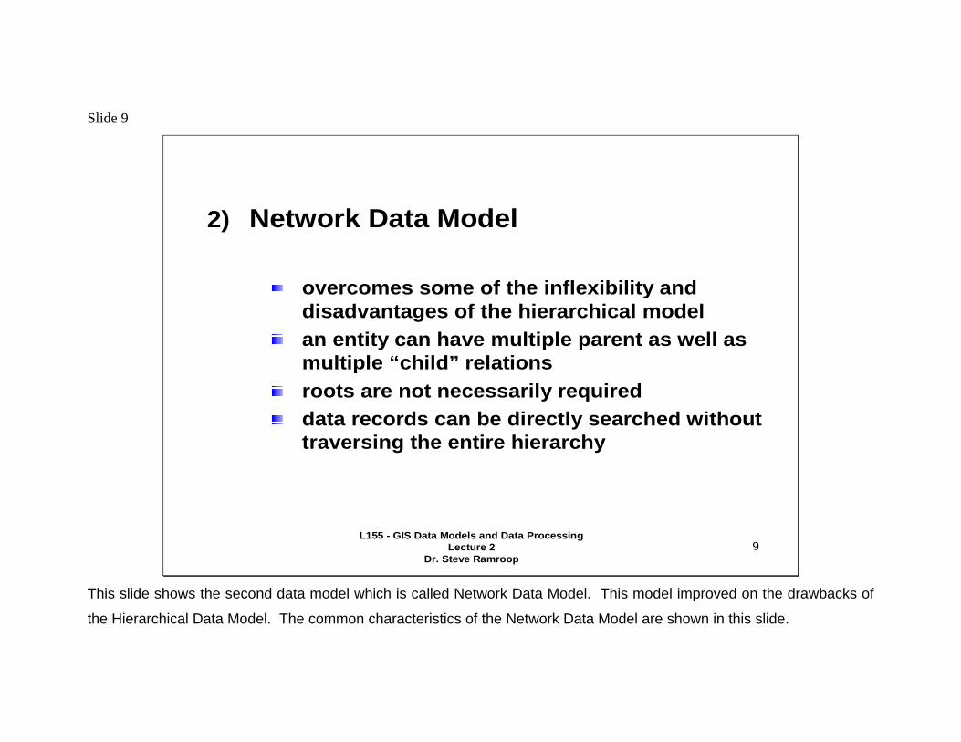
2) Network Data Model
overcomes some of the inflexibility and disadvantages of the hierarchical modelan entity can have multiple parent as well as multiple “child” relations roots are not necessarily requireddata records can be directly searched without traversing the entire hierarchy
This slide shows the second data model which is called Network Data Model. This model improved on the drawbacks of
the Hierarchical Data Model. The common characteristics of the Network Data Model are shown in this slide.
Slide 10
10L155 - GIS Data Models and Data Processing
Lecture 2Dr. Steve Ramroop
> Courses are related to the Department and the Professors
> Registration are related to the Courses and Students
Organization of a database using the Network Data Model
This slide show the same example adopted in the context of University that has professors who teach courses. As shown
in the figure there is a relationship between University and Department; Department and Students; Professors and
courses; and Students and Registration. There are multiple relationships between Courses and Registration. That is,
Courses have a relationship with Professors and also a relationship with Department. Registration has multiple
relationships as well. There is a relation between Registration and Courses; as well as a relationship with Registration
and Students. This entire example is applied using a Network Data Model as shown in the figure.
In the Network Data Model a “child” can have more than one “parent”. That is, in this data model lower levels of the
hierarchy can have multiple higher level relationships. For example “courses” are related to the ‘department’ and
“professors”, and “registration” has a relationship to the “courses” and the “students”.
Slide 11
11L155 - GIS Data Models and Data Processing
Lecture 2Dr. Steve Ramroop
1
2 3
4 5
6
a2
a1
a3
a4
a5
a7
a6
a2a1 a3 a4
a5 a6 a7
AB
A B
MAP
An example:
1 32 4 5 6
This is another graphic representation of how the network data model is applied to a map representation.
The entire Map is shown. The letters A and B are the sections of the Map. Each section is defined by a set of arcs
labeled by a lower case (a) with a sequential numbering as its subscript. An arc is defined by a start node and an end
node. Nodes are labeled at the intersection of arcs and the nodes are numbered sequentially starting from 1 and ending
at 6. Notice that arc a4 is not repeated under sections A and B.
Slide 12
12L155 - GIS Data Models and Data Processing
Lecture 2Dr. Steve Ramroop
Notes on the previous figure (network model example):
no hierarchy of data fields within a record“A” and “B” are parents themselves who
have children “A” has children a1 …. a4
“B” has children a4 …. a7
a4 is NOT repeated
This slide gives some details into the previous slide of the Network Data model.
Slide 13
13L155 - GIS Data Models and Data Processing
Lecture 2Dr. Steve Ramroop
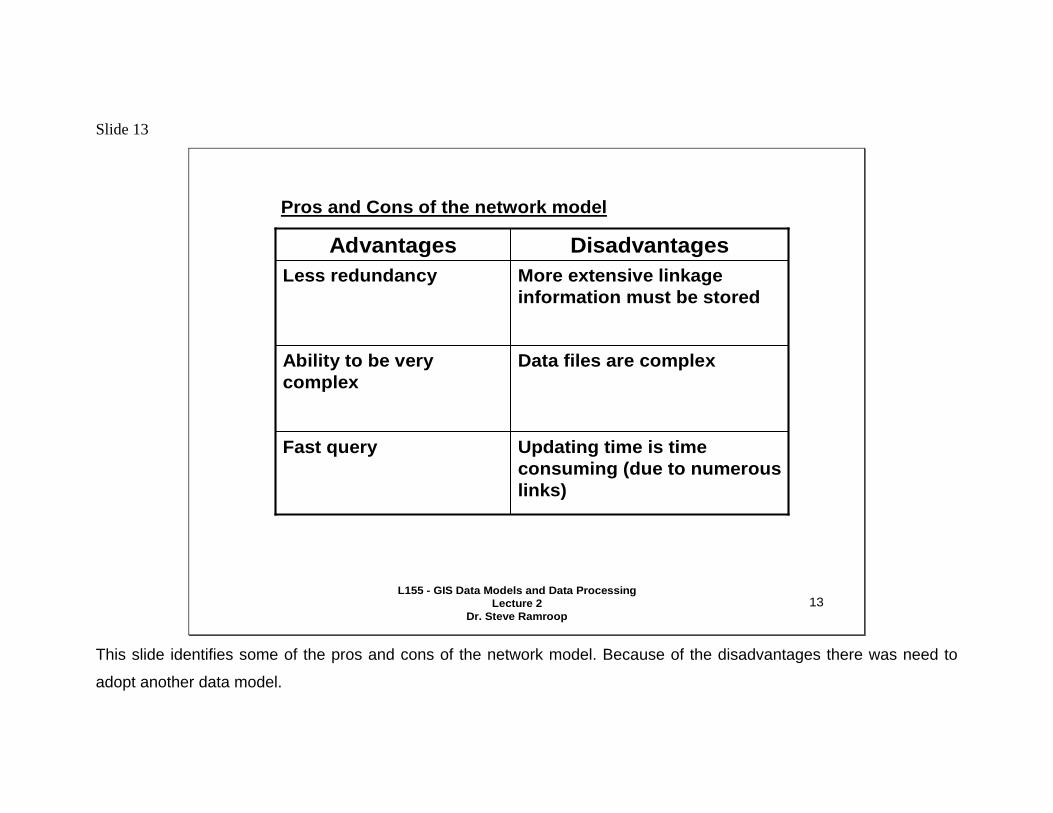
Updating time is time consuming (due to numerous links)
Fast query
Data files are complexAbility to be very complex
More extensive linkage information must be stored
Less redundancyDisadvantagesAdvantages
Pros and Cons of the network model
This slide identifies some of the pros and cons of the network model. Because of the disadvantages there was need to
adopt another data model.
Slide 14
14L155 - GIS Data Models and Data Processing
Lecture 2Dr. Steve Ramroop
3) Relational Data Modelmore popular data models used in GISno hierarchy of data fields within a recordevery data field can be used as a keythe table as a whole represents the relationship among all the attributes it contains in a single table and is often called a “relation”relations are also defined between tables using unique ID numbersData integrity is managed by having many tables with their relations explicitly defined. This is the process called “normalization”
The third data model is presented here -- Relational Data Model. Put simply, it is the ability to define the relationships
between entities using tables that defined the entities. This model maintains data integrity through a process called
normalization. This is the process in which smaller tables are defined to explicitly define the relationships between tables.
This is done in order to maintain data integrity and also facilitate easy updating. Note that every data field in a table can
be used as a key which can be linked to other tables that has the same key definition.
Slide 15
15L155 - GIS Data Models and Data Processing
Lecture 2Dr. Steve Ramroop
– table relationships can be :one to one : one table related to another tablemany to one : many tables related to one tableone to many : one table related to many tablesmany to many : many tables related to many tables
– searches can be made of any single table using any of the attribute fields, singly or together
– to perform searches on different tables, links between them (using any attribute they share in common) must be establishedProcedure is termed “JOIN”
This slide identifies the various relations that can exist between tables. Before queries can be done, tables can be joined
or linked depending upon the existing relationships. GIS software is equipped to represent the relationships between
tables, (called attribute data) that are linked to the map phenomena, (called spatial data).
Slide 16
16L155 - GIS Data Models and Data Processing
Lecture 2Dr. Steve Ramroop
Storage of GIS attribute information in a Relational Database
This is another example of a relational data model that links the spatial data with the attribute data sets. The map is
linked to Attribute Table 1 using the Map ID column as the key. Then Attribute Table 1 is linked to Attribute Table 2 using
the Stand Number column as the key.
Slide 17
17L155 - GIS Data Models and Data Processing
Lecture 2Dr. Steve Ramroop
– need to deal with the “problem” of redundancy of data – usually there is a trade-off into the amount of
redundancy a relational database can have since it affects data storage and the speed at which queries are executed
– note that it takes longer to search the data stored in several tables than to search the same data stored in one table
– However, data stored in one table may also have null entries which is not a good characteristic in databases
– As the number of data tables are reduced, the redundancy of data storage tends to increase
– no restrictions on the type of queries possible (flexible)
Notes on the previous figure (relational model):
This slide gives some self explanatory notes about the relational model. There is the problem of data redundancy in
tables. The goal is to get a good balance as to how much redundancy is allowed for a given GIS application.
Slide 18
18L155 - GIS Data Models and Data Processing
Lecture 2Dr. Steve Ramroop
4) Object Oriented Data (OOD) Model– everything in the real world is considered an
object– each object has its own data plus the program
code for accessing or altering the information– Object Oriented Data Model is based upon the
following context (called abstraction processes):
a) Aggregation - transforming relations to a higher levelb) Classification - abstracting common characteristics of
objectsc) Generalization - placing classes into a hierarchy of
classes
This is the forth data model. This is slowly becoming popular. We are moving towards treating every real world entity as
an object, which can have a state, and is capable of being classified.
Slide 19
19L155 - GIS Data Models and Data Processing
Lecture 2Dr. Steve Ramroop
left right
Segments start
endPoints Nodes
Objects
Map
An example:
To form a map using the OOD model, nodes and points are used. They can also be used to define segments which can be left or right as in the case of polygons to form objects of the overall map
This is a graphical representation of how OOD model is used to represent map entities. Segments can be aggregated to
form objects. Each segments has a start and end node. The collection of segments, nodes, and points are use to
represent the map.
Slide 20
20L155 - GIS Data Models and Data Processing
Lecture 2Dr. Steve Ramroop
5) Temporal Model
involves the ability to attach time data and its time dimensionthis is one of the recent areas of research and different approaches are being researched to find the ability to maintain / record the time dimensionparticularly useful for cadastral systems where there is a need to register the changes of land ownership and other historical characteristics
This is the fifth data model. It is an area of ongoing research. It is associated with the attachment of time stamps to the