WHITEPAPER

Data Preparation in Angoss Analytics Software Suite Technical Whitepaper May 2012

2

Table of Contents 1. Overview ............................................................................................................................ 3

2. Dataset-level and Row-level Manipulations ........................................................................ 5

2.1. Joining Datasets ........................................................................................................... 5

2.2. Removing Duplicate Records ....................................................................................... 9

2.3. Appending Datasets ....................................................................................................11

2.4. Aggregating Data ........................................................................................................15

3. Column-level Transformations ...........................................................................................19

3.1. Expression Editor ........................................................................................................19

3.2. Importing and Exporting Calculated Columns ..............................................................21

3.3. Calculated Columns in the In-Database Analytics Mode .............................................21

3.4. Expression Helpers .....................................................................................................22

3.5. Helper Examples .........................................................................................................24

About Angoss Software .........................................................................................................28

3

1. Overview Upon importing data or connecting to a database table using the In-Database Analytics driver, you normally need to prepare the data for analysis if you have not already done so in the data source.

Data preparation in KnowledgeSEEKER and KnowledgeSTUDIO includes two types of data transformation:

a) Dataset-level and row-level manipulations are performed using the Data menu commands: joining, appending, and aggregating datasets, as well as removing duplicate records.

b) Column-level transformations: Adding calculated columns using SQL expressions in the Dataset Editor.

All data preparation operations are supported both for Angoss datasets and for database tables in the In-Database Analytics mode.

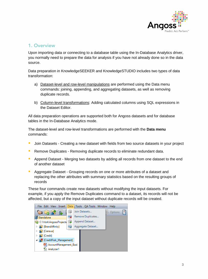
The dataset-level and row-level transformations are performed with the Data menu commands:

Join Datasets - Creating a new dataset with fields from two source datasets in your project

Remove Duplicates - Removing duplicate records to eliminate redundant data.

Append Dataset - Merging two datasets by adding all records from one dataset to the end of another dataset

Aggregate Dataset - Grouping records on one or more attributes of a dataset and replacing the other attributes with summary statistics based on the resulting groups of records

These four commands create new datasets without modifying the input datasets. For example, if you apply the Remove Duplicates command to a dataset, its records will not be affected, but a copy of the input dataset without duplicate records will be created.

4

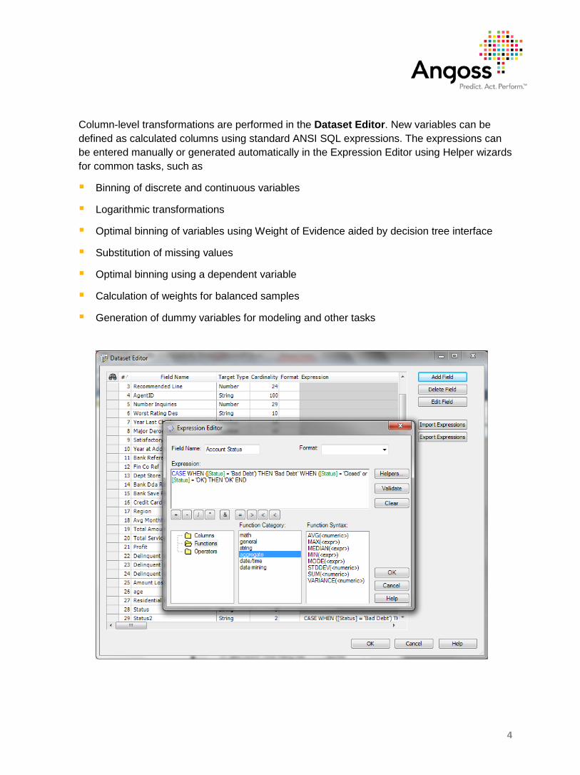
Column-level transformations are performed in the Dataset Editor. New variables can be defined as calculated columns using standard ANSI SQL expressions. The expressions can be entered manually or generated automatically in the Expression Editor using Helper wizards for common tasks, such as

Binning of discrete and continuous variables

Logarithmic transformations

Optimal binning of variables using Weight of Evidence aided by decision tree interface

Substitution of missing values

Optimal binning using a dependent variable

Calculation of weights for balanced samples

Generation of dummy variables for modeling and other tasks

5

2. Dataset-level and Row-level Manipulations

2.1. Joining Datasets

Datasets containing different information about related entities often need to be joined in a single dataset for analysis. The joining is possible if the datasets have at least one common attribute that serves as a link.

For example, retail transaction data and customer demographics data often come from two different sources, but each contains a customer ID field that can be used to link them together.

The Join Datasets command under the Data menu allows you to create a new dataset with fields from two source datasets in your project. By consecutively joining pairs of datasets, you can create a single dataset for analysis from many different input sources.

The command is also applicable to tables in the In-Database mode if you have the In-Database Analytics add-on license.

The Join Dataset command launches a wizard that lets you choose the source datasets, specify the link - a single field that contains an identifier present in both datasets - and choose the attributes from each source dataset to be included in the new dataset. You can also specify which records to include in the output – only records that appear in both datasets, or all records from one of the source datasets.

The Join Datasets Wizard

To join two datasets, open your project and select the command Data | Join Datasets from the menu.

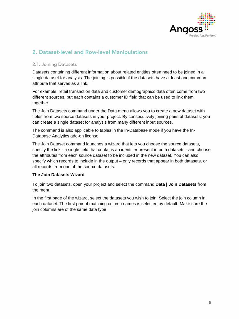
In the first page of the wizard, select the datasets you wish to join. Select the join column in each dataset. The first pair of matching column names is selected by default. Make sure the join columns are of the same data type

6

In the above example, we chose to join a dataset with campaign responses and a dataset with demographics data for customers in a retail company’s loyalty program. Both datasets have a loyalty card ID field. This will be useful to build a response model with demographics attributes as independent variables.

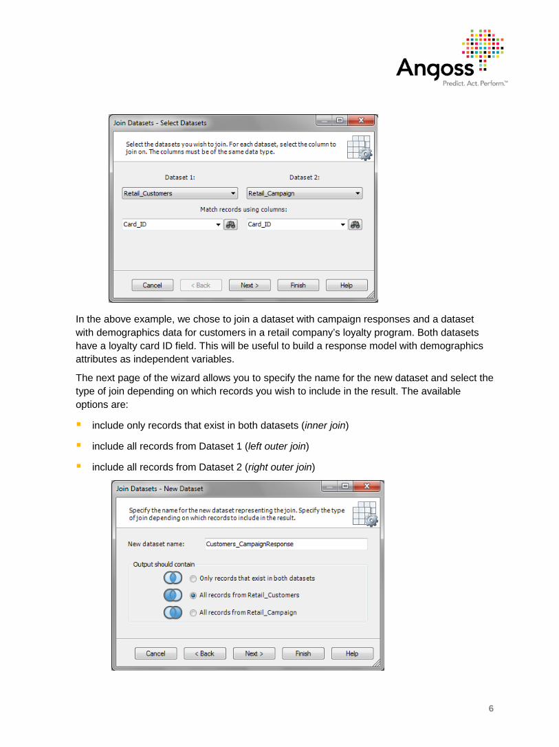
The next page of the wizard allows you to specify the name for the new dataset and select the type of join depending on which records you wish to include in the result. The available options are:

include only records that exist in both datasets (inner join)

include all records from Dataset 1 (left outer join)

include all records from Dataset 2 (right outer join)

7

In the case where all records from one of the datasets are included (left or right outer join), any records that do not match will have null values inserted for attributes from the unmatched side of the join.

The default output dataset name is the concatenation of the two source dataset names with an underscore in between. It can be modified if necessary.

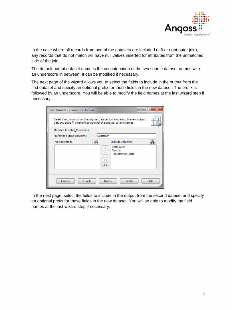
The next page of the wizard allows you to select the fields to include in the output from the first dataset and specify an optional prefix for these fields in the new dataset. The prefix is followed by an underscore. You will be able to modify the field names at the last wizard step if necessary.

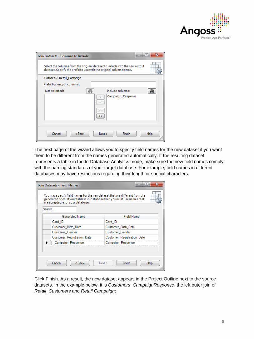
In the next page, select the fields to include in the output from the second dataset and specify an optional prefix for these fields in the new dataset. You will be able to modify the field names at the last wizard step if necessary.

8

The next page of the wizard allows you to specify field names for the new dataset if you want them to be different from the names generated automatically. If the resulting dataset represents a table in the In-Database Analytics mode, make sure the new field names comply with the naming standards of your target database. For example, field names in different databases may have restrictions regarding their length or special characters.

Click Finish. As a result, the new dataset appears in the Project Outline next to the source datasets. In the example below, it is Customers_CampaignResponse, the left outer join of Retail_Customers and Retail Campaign:

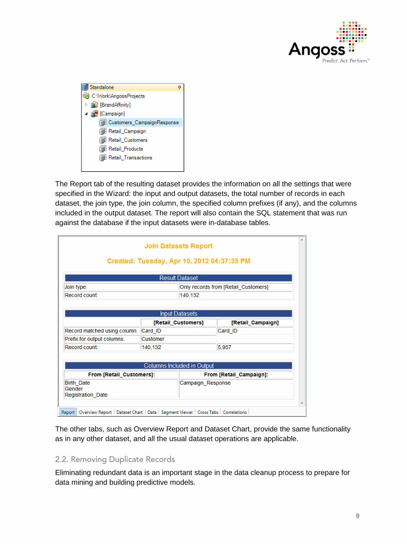
9

The Report tab of the resulting dataset provides the information on all the settings that were specified in the Wizard: the input and output datasets, the total number of records in each dataset, the join type, the join column, the specified column prefixes (if any), and the columns included in the output dataset. The report will also contain the SQL statement that was run against the database if the input datasets were in-database tables.

The other tabs, such as Overview Report and Dataset Chart, provide the same functionality as in any other dataset, and all the usual dataset operations are applicable.

2.2. Removing Duplicate Records

Eliminating redundant data is an important stage in the data cleanup process to prepare for data mining and building predictive models.

10

For example, unwanted duplicate records may occur in the dataset resulting from merging data from many sources using the Append operation.

To remove records that contain duplicate entries, open the project that contains the dataset in question and select the Remove Duplicates command from the Data menu.

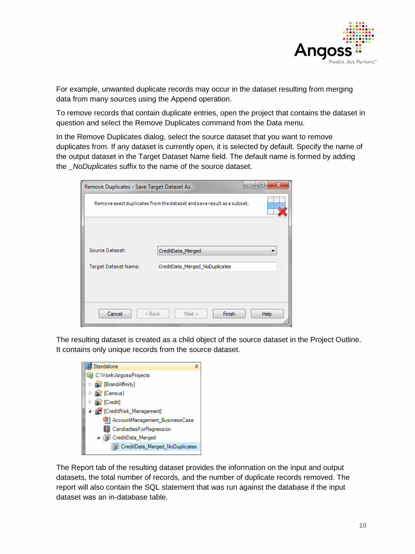
In the Remove Duplicates dialog, select the source dataset that you want to remove duplicates from. If any dataset is currently open, it is selected by default. Specify the name of the output dataset in the Target Dataset Name field. The default name is formed by adding the _NoDuplicates suffix to the name of the source dataset.

The resulting dataset is created as a child object of the source dataset in the Project Outline. It contains only unique records from the source dataset.

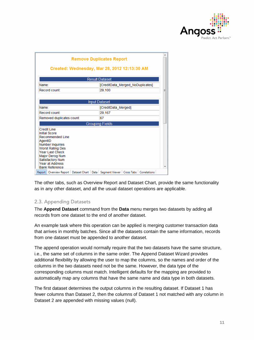
The Report tab of the resulting dataset provides the information on the input and output datasets, the total number of records, and the number of duplicate records removed. The report will also contain the SQL statement that was run against the database if the input dataset was an in-database table.

11

The other tabs, such as Overview Report and Dataset Chart, provide the same functionality as in any other dataset, and all the usual dataset operations are applicable.

2.3. Appending Datasets The Append Dataset command from the Data menu merges two datasets by adding all records from one dataset to the end of another dataset.

An example task where this operation can be applied is merging customer transaction data that arrives in monthly batches. Since all the datasets contain the same information, records from one dataset must be appended to another dataset.

The append operation would normally require that the two datasets have the same structure, i.e., the same set of columns in the same order. The Append Dataset Wizard provides additional flexibility by allowing the user to map the columns, so the names and order of the columns in the two datasets need not be the same. However, the data type of the corresponding columns must match. Intelligent defaults for the mapping are provided to automatically map any columns that have the same name and data type in both datasets.

The first dataset determines the output columns in the resulting dataset. If Dataset 1 has fewer columns than Dataset 2, then the columns of Dataset 1 not matched with any column in Dataset 2 are appended with missing values (null).

12

The Append Dataset Wizard

To append a dataset to another one, open your project and select the command Data | Append Dataset from the menu.

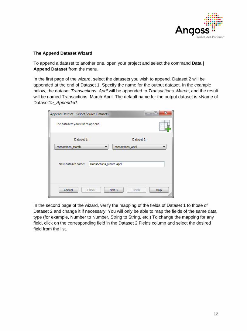
In the first page of the wizard, select the datasets you wish to append. Dataset 2 will be appended at the end of Dataset 1. Specify the name for the output dataset. In the example below, the dataset Transactions_April will be appended to Transactions_March, and the result will be named Transactions_March-April. The default name for the output dataset is <Name of Dataset1>_Appended.

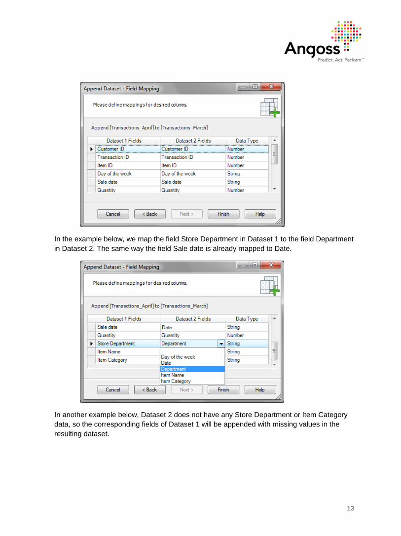
In the second page of the wizard, verify the mapping of the fields of Dataset 1 to those of Dataset 2 and change it if necessary. You will only be able to map the fields of the same data type (for example, Number to Number, String to String, etc.) To change the mapping for any field, click on the corresponding field in the Dataset 2 Fields column and select the desired field from the list.

13

In the example below, we map the field Store Department in Dataset 1 to the field Department in Dataset 2. The same way the field Sale date is already mapped to Date.

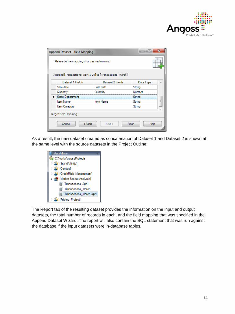
In another example below, Dataset 2 does not have any Store Department or Item Category data, so the corresponding fields of Dataset 1 will be appended with missing values in the resulting dataset.

14

As a result, the new dataset created as concatenation of Dataset 1 and Dataset 2 is shown at the same level with the source datasets in the Project Outline:

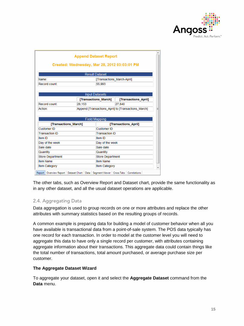
The Report tab of the resulting dataset provides the information on the input and output datasets, the total number of records in each, and the field mapping that was specified in the Append Dataset Wizard. The report will also contain the SQL statement that was run against the database if the input datasets were in-database tables.

15

The other tabs, such as Overview Report and Dataset chart, provide the same functionality as in any other dataset, and all the usual dataset operations are applicable.

2.4. Aggregating Data Data aggregation is used to group records on one or more attributes and replace the other attributes with summary statistics based on the resulting groups of records.

A common example is preparing data for building a model of customer behavior when all you have available is transactional data from a point-of-sale system. The POS data typically has one record for each transaction. In order to model at the customer level you will need to aggregate this data to have only a single record per customer, with attributes containing aggregate information about their transactions. This aggregate data could contain things like the total number of transactions, total amount purchased, or average purchase size per customer.

The Aggregate Dataset Wizard

To aggregate your dataset, open it and select the Aggregate Dataset command from the Data menu.

16

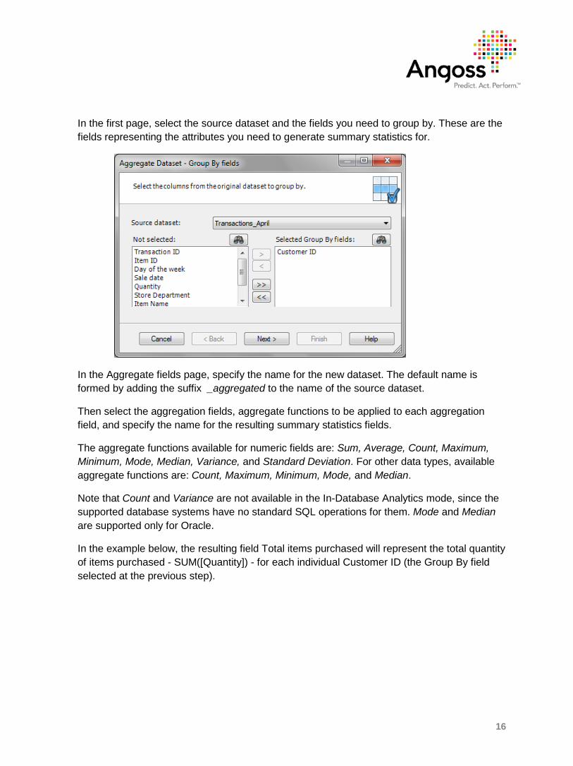
In the first page, select the source dataset and the fields you need to group by. These are the fields representing the attributes you need to generate summary statistics for.

In the Aggregate fields page, specify the name for the new dataset. The default name is formed by adding the suffix _aggregated to the name of the source dataset.

Then select the aggregation fields, aggregate functions to be applied to each aggregation field, and specify the name for the resulting summary statistics fields.

The aggregate functions available for numeric fields are: Sum, Average, Count, Maximum, Minimum, Mode, Median, Variance, and Standard Deviation. For other data types, available aggregate functions are: Count, Maximum, Minimum, Mode, and Median.

Note that Count and Variance are not available in the In-Database Analytics mode, since the supported database systems have no standard SQL operations for them. Mode and Median are supported only for Oracle.

In the example below, the resulting field Total items purchased will represent the total quantity of items purchased - SUM([Quantity]) - for each individual Customer ID (the Group By field selected at the previous step).

17

As a result, the new aggregated dataset is shown in the Project Outline at the same hierarchical level with the source dataset:

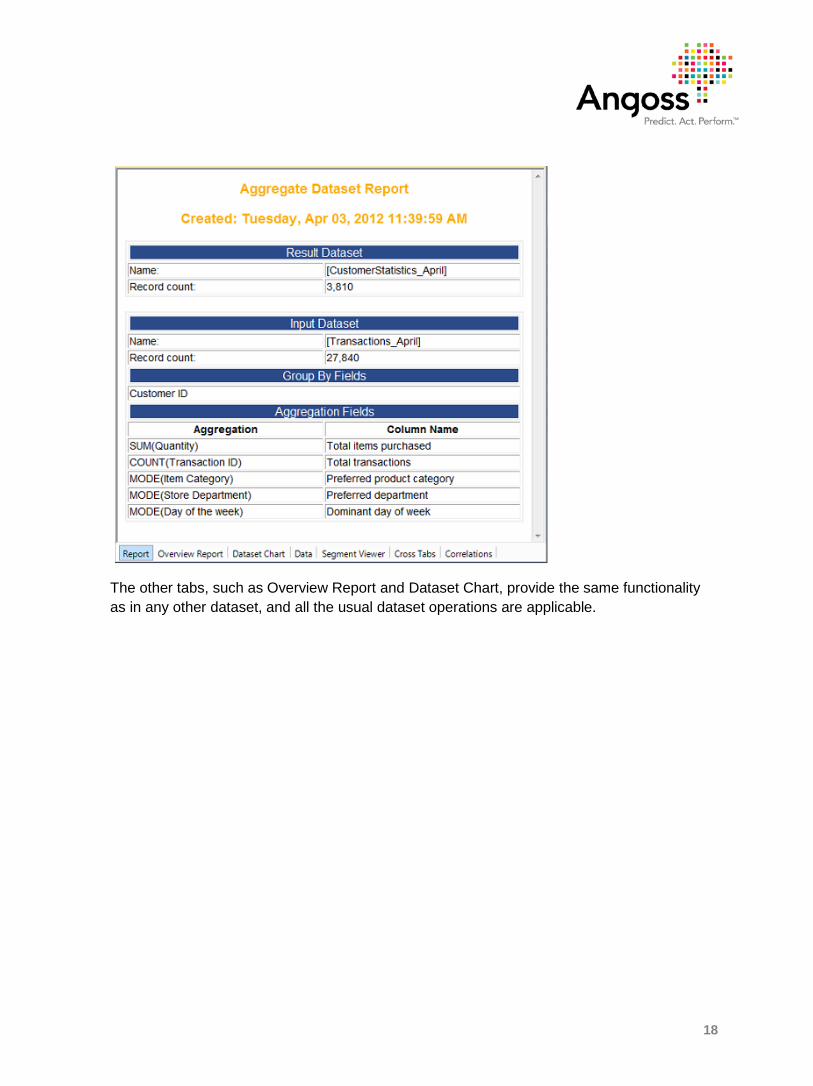
The Report tab of the resulting dataset provides the information on the input and output datasets, the total number of records in each, the Group By field, and the aggregation fields that were specified in the Aggregate Dataset Wizard. The report will also contain the SQL statement that was run against the database if the input dataset was an in-database table.

18

The other tabs, such as Overview Report and Dataset Chart, provide the same functionality as in any other dataset, and all the usual dataset operations are applicable.

19

3. Column-level Transformations

Column-level transformations are often necessary to derive attributes more suitable for analysis and predictive modeling. For example, simple transformations can help you substitute custom values for missing values, discretize continuous variables, map the values of a categorical variable into a smaller set of values, etc.

Dataset Editor provides the following capabilities for manipulating columns in datasets:

adding new calculated columns

deleting columns

editing expressions for existing calculated columns

specifying display format and precision for any column (Currency, Percent, etc.)

importing expressions for calculated columns from other datasets or expression files

Dataset Editor is invoked by the menu command Tools | Dataset Editor.

3.1. Expression Editor The Expression Editor is a tool within the Dataset Editor that allows you to build expressions for creating new calculated columns in your dataset. Some of the common objectives for creating a new column are:

mapping the categories of a discrete field to new categories

merging several categories into one

creating a discrete representation (binning) of a continuous variable

replacing missing values

creating dummy variables

performing logarithmic and power transformations, etc.

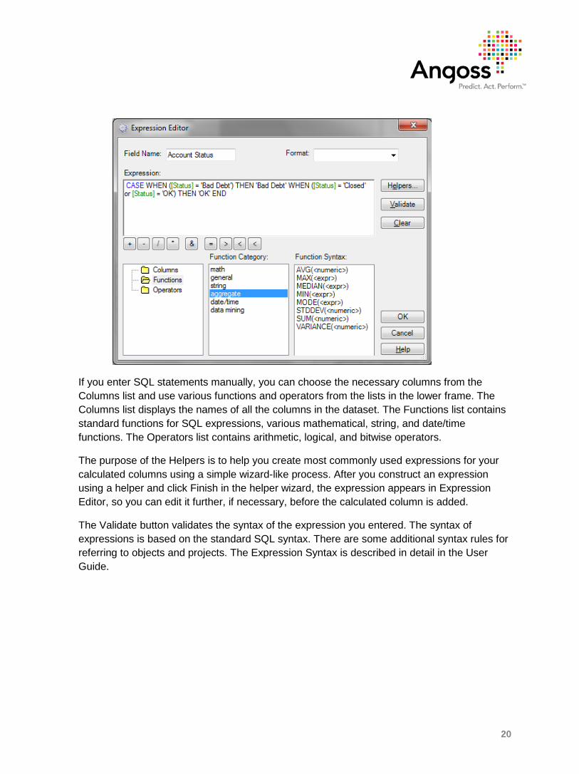
The Expression Editor is invoked by clicking the Add Field or Edit Field button in the Dataset Editor dialog. It allows you to manually enter SQL expressions or use intuitive wizards called Helpers to create most common types of expressions. The screenshot below illustrates an example of merging two values of a discrete variable into one (the categories ‘Closed’ and ‘OK’ are merged into one category called ‘OK’, while ‘Bad Debt’ remains the same):

20

If you enter SQL statements manually, you can choose the necessary columns from the Columns list and use various functions and operators from the lists in the lower frame. The Columns list displays the names of all the columns in the dataset. The Functions list contains standard functions for SQL expressions, various mathematical, string, and date/time functions. The Operators list contains arithmetic, logical, and bitwise operators.

The purpose of the Helpers is to help you create most commonly used expressions for your calculated columns using a simple wizard-like process. After you construct an expression using a helper and click Finish in the helper wizard, the expression appears in Expression Editor, so you can edit it further, if necessary, before the calculated column is added.

The Validate button validates the syntax of the expression you entered. The syntax of expressions is based on the standard SQL syntax. There are some additional syntax rules for referring to objects and projects. The Expression Syntax is described in detail in the User Guide.

21

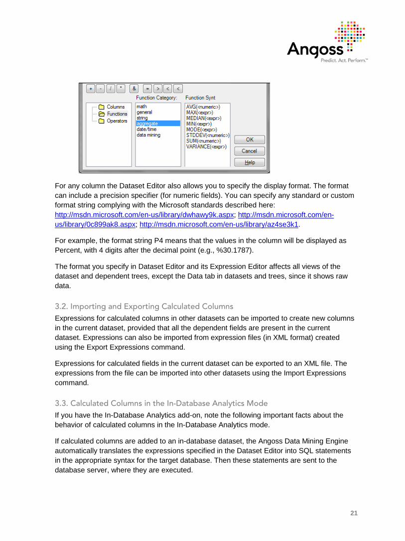
For any column the Dataset Editor also allows you to specify the display format. The format can include a precision specifier (for numeric fields). You can specify any standard or custom format string complying with the Microsoft standards described here: http://msdn.microsoft.com/en-us/library/dwhawy9k.aspx; http://msdn.microsoft.com/en-us/library/0c899ak8.aspx; http://msdn.microsoft.com/en-us/library/az4se3k1.

For example, the format string P4 means that the values in the column will be displayed as Percent, with 4 digits after the decimal point (e.g., %30.1787).

The format you specify in Dataset Editor and its Expression Editor affects all views of the dataset and dependent trees, except the Data tab in datasets and trees, since it shows raw data.

3.2. Importing and Exporting Calculated Columns Expressions for calculated columns in other datasets can be imported to create new columns in the current dataset, provided that all the dependent fields are present in the current dataset. Expressions can also be imported from expression files (in XML format) created using the Export Expressions command.

Expressions for calculated fields in the current dataset can be exported to an XML file. The expressions from the file can be imported into other datasets using the Import Expressions command.

3.3. Calculated Columns in the In-Database Analytics Mode If you have the In-Database Analytics add-on, note the following important facts about the behavior of calculated columns in the In-Database Analytics mode.

If calculated columns are added to an in-database dataset, the Angoss Data Mining Engine automatically translates the expressions specified in the Dataset Editor into SQL statements in the appropriate syntax for the target database. Then these statements are sent to the database server, where they are executed.

22

SQL expressions defining calculated columns in an in-database dataset are stored locally rather than with the underlying database table. Therefore, if the values in the corresponding columns of the underlying table are modified directly on the database server, these changes will not be reflected in the expressions stored by the Angoss application.

Note that not all of the functions supported in SQL DMX used by Angoss have standard equivalents in the SQL of all supported databases. For Teradata, Microsoft SQL Server and Netezza, the following standard functions are not available: Unique Count, Variance, DevSqr, Mode (Mode1 and Mode2), Lower Quartile, Upper Quartile, and Median. For Oracle, the functions for Variance, DevSqr, Mode and Median are supported for numeric and date/time columns only. Unique Count, Lower Quartile, and Upper Quartile are not supported. The results of calculations with unsupported functions will be undefined (null).

Fields of types Time and Timestamp in Teradata are not supported by Angoss In-Database Analytics, and any calculations with such fields will have an undefined result.

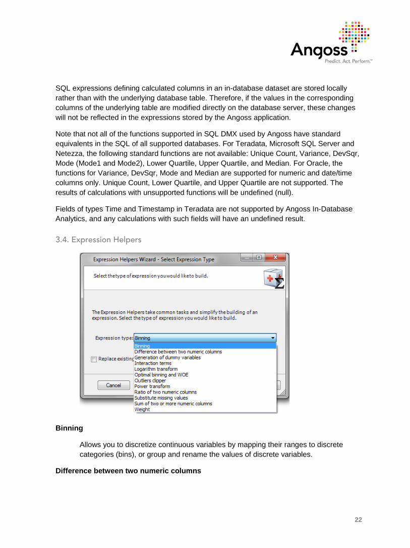
3.4. Expression Helpers

Binning

Allows you to discretize continuous variables by mapping their ranges to discrete categories (bins), or group and rename the values of discrete variables.

Difference between two numeric columns

23

Allows you to subtract the values in one column from the values in another column. See the section “Difference between two numeric columns”.

Ratio of two numeric columns

Allows you to compute the ratio of the values in two numeric columns.

Sum of two or more numeric columns

Allows you to sum the values in two or more numeric columns.

Generation of Dummy Variables

Allows you to create a set of dummy, or indicator variables from a discrete variable. A single column with several string values is transformed into a series of binary columns with values 0 and 1.

Note that, as a part of normalization process in predictive and cluster model training, all String variables are automatically transformed into a set of indicator variables. The helper allows you to do this explicitly, outside of the model building process.

Logarithm transform

Allows you to compute the logarithm of the values in a given column.

Power transform

Allows you to raise the values in a given column to a power.

Substitute missing values

Allows you to substitute a value for all missing values in a column.

Outliers clipper

Allows you to set the new minimum and maximum values and assign the outliers to the new minimum and maximum.

Interaction terms

Allows you to create the products of various combinations of a fixed number of selected variables or their squares. See the Interaction Terms section for details.

Optimal binning and WOE (Weight Of Evidence)

Allows you to create binning transformations that are optimal in terms of providing the highest information value with respect to a given dependent variable. This helper allows you to transform many variables at the same time. It is especially convenient at

24

the coarse classing stage of building scorecards. See the Optimal Binning and WOE section for details.

Weight

The Weight Helper provides a simple and convenient way to add a weight as a calculated column based on the values of any discrete variable. See the section Helper: Weight for details.

3.5. Helper Examples

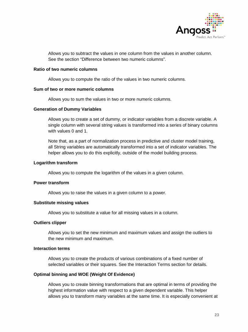
1. Binning Helper

The Binning helper allows you to discretize continuous variables and change or group the values of discrete variables.

Continuous Binning merges the ranges of a continuous variable into discrete values. Discrete Transform maps the values of a discrete variable to the user-specified values. The Range Editor helps you group and assign intervals or discrete values and assign them to the new bins.

Click Next to edit the bins of the selected variable in the Range Editor dialog.

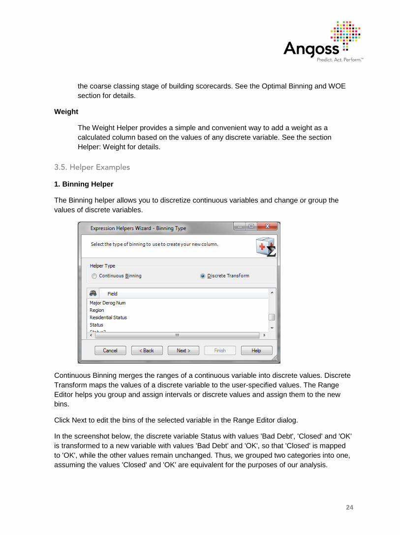
In the screenshot below, the discrete variable Status with values 'Bad Debt', 'Closed' and 'OK' is transformed to a new variable with values 'Bad Debt' and 'OK', so that 'Closed' is mapped to 'OK', while the other values remain unchanged. Thus, we grouped two categories into one, assuming the values 'Closed' and 'OK' are equivalent for the purposes of our analysis.

25

Click Next to generate the expression and preview it.

Then Click Finish to add the expression and return to Expression Editor

2. Generation of Dummy Variables

This helper allows you to create a set of dummy, or indicator variables from a discrete variable. Based on a single discrete column, it creates a series of binary variables with values 0 and 1.

26

For example, if a variable called Status in a credit account dataset has values "OK", "Bad Debt", and "Closed", the helper transforms it into the set of three dummy variables with values 0 and 1 indicating the value taken by the original Status variable.

Status Status_OK Status_Bad Debt Status_Closed

OK 1 0 0

Bad Debt 0 1 0

Closed 0 0 1

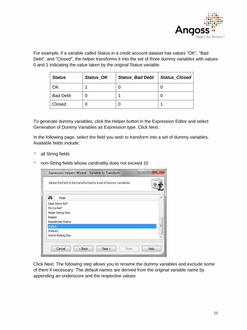
To generate dummy variables, click the Helper button in the Expression Editor and select Generation of Dummy Variables as Expression type. Click Next.

In the following page, select the field you wish to transform into a set of dummy variables. Available fields include:

all String fields

non-String fields whose cardinality does not exceed 10

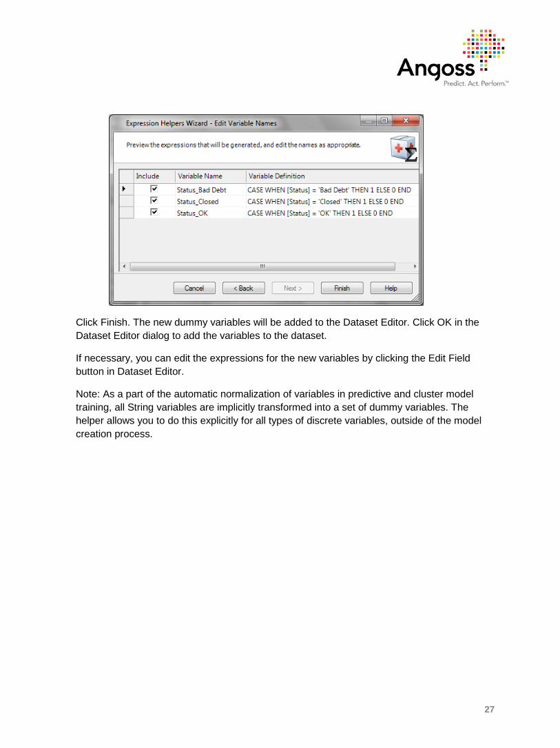
Click Next. The following step allows you to rename the dummy variables and exclude some of them if necessary. The default names are derived from the original variable name by appending an underscore and the respective values

27

Click Finish. The new dummy variables will be added to the Dataset Editor. Click OK in the Dataset Editor dialog to add the variables to the dataset.

If necessary, you can edit the expressions for the new variables by clicking the Edit Field button in Dataset Editor.

Note: As a part of the automatic normalization of variables in predictive and cluster model training, all String variables are implicitly transformed into a set of dummy variables. The helper allows you to do this explicitly for all types of discrete variables, outside of the model creation process.

28

About Angoss Software As a global leader in predictive analytics, Angoss helps businesses increase sales and profitability, and reduce risk. Angoss helps businesses discover valuable insight and intelligence from their data while providing clear and detailed recommendations on the best and most profitable opportunities to pursue to improve sales, marketing and risk performance.

Our suite of desktop, client-server and in-database software products and Cloud solutions make predictive analytics accessible and easy to use for technical and business users. Many of the world's leading organizations use Angoss software products and solutions to grow revenue, increase sales productivity and improve marketing effectiveness while reducing risk and cost.

Corporate Headquarters European Headquarters

111 George Street, Suite 200 Toronto, Ontario M5A 2N4 Canada Tel: 416-593-1122 Fax: 416-593-5077

www.angoss.com

Surrey Technology Centre 40 Occam Road The Surrey Research Park Guildford, Surrey GU2 7YG Tel: +44 (0) 1483-685-770

© Copyright 2013. Angoss Software Corporation – www.angoss.com