Data-Quality Improvements and Applications of Long-Term Monitoring of Ionospheric Anomalies for GBAS Minchan Kim Korea Advanced Institute of Science and Technology* Jiyun Lee* Tetra Tech AMT Sam Pullen Stanford University and Joseph Gillespie William J. Hughes FAA Technical Center ABSTRACT The Long-Term Ionospheric Anomaly Monitoring (LTIAM) tool is an automated software package designed to analyze past data and support continuous ionospheric monitoring of both nominal and anomalous ionospheric spatial gradients. While automated measurement screening is included, large gradients observed by LTIAM require manual validation to confirm that they were caused by the ionosphere instead of faulty measurements or data recording. Ground stations with poor data quality thus add greatly to the burden of LTIAM processing. This paper develops an automated approach to data quality measurement for CORS and IGS ground stations. This method is used to identify stations that are poor according to multiple quality metrics. Thresholds are established for each quality metric, and stations violating one or more thresholds are removed from use by LTIAM unless their geographical position is sufficiently important. Use of this method with CORS stations in the Conterminous U.S. (CONUS) eliminates the almost 90% of spurious or false gradients while only excluding 16% of the over 1500 CORS stations in CONUS. This paper also investigates past CONUS ionospheric storm data to understand the distribution of anomalous spatial gradients. Examining LTIAM outputs on known storm days with gradients between 50 and 200 mm/km demonstrates that these smaller (but still anomalous) gradients are far more likely than extreme gradients above 200 mm/km. The continued use of LTIAM over the next solar peak should help us refine our knowledge of this distribution as well as the overall likelihood of large spatial gradients under anomalous ionospheric conditions. 1.0. INTRODUCTION An automated Long-Term Ionospheric Anomaly Monitoring (LTIAM) software package has been developed to support continuous ionospheric monitoring for the U.S. Local Area Augmentation System (LAAS) developed by the U.S. Federal Aviation Administration (FAA) in the Conterminous U.S. (CONUS). Continuous monitoring is needed to confirm the long-term validity of existing ionospheric threat models and support updates if necessary. This is of particular importance over the next few years, as the intensity of solar storms is expected to peak in 2013-15. Continuous monitoring using the LTIAM provides reliable ionospheric gradient statistics under typical as well as anomalous conditions. The LTIAM will also be utilized to build threat models for other regions where Ground-Based Augmentation Systems (GBAS) will be fielded. The LTIAM software enables automated post-processing of data continuously collected by GPS reference station networks. Ionospheric gradients over short-baseline distances of 5 – 40 km can be observed using data collected from the Continuously Operating Reference Stations (CORS) network, which has over 1800 stations as of 2011 in the U.S. territories and a few other countries compared to about 400 stations prior to 2004. However, as the total number of stations increases, the number of stations with poor GPS data quality also increases. CORS receivers and antennas are fielded by multiple organizations in various environments; some good, some not-so-good. Poor-quality data degrades the accuracy of ionospheric delay estimates and produces too many faulty anomaly candidates, meaning apparent anomalies that are actually due to measurement or data errors.
Transcript
Data-Quality Improvements and Applications of Long-Term Monitoring of
Ionospheric Anomalies for GBAS
Minchan Kim Korea Advanced Institute of Science and Technology*
Jiyun Lee* Tetra Tech AMT
Sam Pullen Stanford University
and Joseph Gillespie
William J. Hughes FAA Technical Center
ABSTRACT The Long-Term Ionospheric Anomaly Monitoring (LTIAM) tool is an automated software package designed to analyze past data and support continuous ionospheric monitoring of both nominal and anomalous ionospheric spatial gradients. While automated measurement screening is included, large gradients observed by LTIAM require manual validation to confirm that they were caused by the ionosphere instead of faulty measurements or data recording. Ground stations with poor data quality thus add greatly to the burden of LTIAM processing. This paper develops an automated approach to data quality measurement for CORS and IGS ground stations. This method is used to identify stations that are poor according to multiple quality metrics. Thresholds are established for each quality metric, and stations violating one or more thresholds are removed from use by LTIAM unless their geographical position is sufficiently important. Use of this method with CORS stations in the Conterminous U.S. (CONUS) eliminates the almost 90% of spurious or false gradients while only excluding 16% of the over 1500 CORS stations in CONUS. This paper also investigates past CONUS ionospheric storm data to understand the distribution of anomalous spatial gradients. Examining LTIAM outputs on known storm days with gradients between 50 and 200 mm/km demonstrates that these smaller (but still anomalous) gradients are far more likely than extreme gradients above 200 mm/km. The continued use of LTIAM over the next solar peak should help us refine our knowledge of this distribution as well as the overall likelihood of large spatial gradients under anomalous ionospheric conditions.
1.0. INTRODUCTION An automated Long-Term Ionospheric Anomaly Monitoring (LTIAM) software package has been developed to support continuous ionospheric monitoring for the U.S. Local Area Augmentation System (LAAS) developed by the U.S. Federal Aviation Administration (FAA) in the Conterminous U.S. (CONUS). Continuous monitoring is needed to confirm the long-term validity of existing ionospheric threat models and support updates if necessary. This is of particular importance over the next few years, as the intensity of solar storms is expected to peak in 2013-15. Continuous monitoring using the LTIAM provides reliable ionospheric gradient statistics under typical as well as anomalous conditions. The LTIAM will also be utilized to build threat models for other regions where Ground-Based Augmentation Systems (GBAS) will be fielded. The LTIAM software enables automated post-processing of data continuously collected by GPS reference station networks. Ionospheric gradients over short-baseline distances of 5 – 40 km can be observed using data collected from the Continuously Operating Reference Stations (CORS) network, which has over 1800 stations as of 2011 in the U.S. territories and a few other countries compared to about 400 stations prior to 2004. However, as the total number of stations increases, the number of stations with poor GPS data quality also increases. CORS receivers and antennas are fielded by multiple organizations in various environments; some good, some not-so-good. Poor-quality data degrades the accuracy of ionospheric delay estimates and produces too many faulty anomaly candidates, meaning apparent anomalies that are actually due to measurement or data errors.
This paper presents a comprehensive method of GPS data quality determination to select CORS stations with high-quality data. A series of algorithms provide information about measurement quality, including cycle slips, receiver noise and multipath, and the daily number of observations (including measurement gaps). Cycle slip detection methods already developed as a part of LTIAM pre-processing have been upgraded by incorporating cycle slips detected using multipath estimates. Multipath on code observations is computed by linear combinations of L1 C/A-code, L1 P-code, and L2 P-code observations. Carrier multipath and receiver noise are estimated using an adaptive filter algorithm. Thresholds are derived for each of these metrics, and stations which lie outside the threshold of one or more metrics are excluded from LTIAM measurement processing unless they are recovered by a secondary check on their location. Stations whose location for observing the ionosphere is sufficiently important are retained despite poor data quality. When implemented on recent CORS station data in CONUS on nominal ionospheric days, the removal of relatively few stations is needed to dramatically reduce the number of false anomaly outputs from LTIAM. The results are more reliable LTIAM results and a reduced manual analysis burden in examining the remaining apparent anomalies. In this paper, Section 3.0 illustrates the problem of poor data quality; Section 4.0 explains the automated data-quality analysis methodology in detail, and Section 5.0 shows the results of applying this method to CORS stations in CONUS. The upgraded LTIAM software allows us to better understand past ionospheric anomalies as well as monitor future ones. This paper re-examines the record of ionospheric “storm” days in CONUS from 2000-2005 to better understand the distribution of spatial gradients under anomalous ionospheric conditions. This database has been thoroughly searched manually and by earlier versions of LTIAM for “extreme” gradients above 200 mm/km that drive the GBAS threat space and have the potential for harm. Here, this database is searched for less-extreme gradients between 50 and 200 mm/km that are still anomalous but much less threatening to GBAS. As expected, far more gradients are found at these lower levels, and within this range, lower gradients are more probable than higher ones. Section 6.0 describes this analysis and explains how to update it with future data, and Section 7.0 concludes the paper. 2.0. LTIAM OVERVIEW The methodology for automated long-term ionospheric observation and anomaly monitoring (LTIAM) has been developed based on the data analysis and verification techniques used to generate the CONUS ionospheric
threat model using manual data processing, as described in [1,2]. Long-term monitoring is required to continually monitor ionospheric behavior as long as GBAS is dependent on the outer bounds of ionospheric threat models, particularly the maximum possible ionospheric spatial gradients. The LTIAM tool will be used to evaluate the validity of the current threat model over the life cycle of system and update it if necessary. It also supports monitoring of gradients under nominal ionospheric conditions, which are bounded by the broadcast value of vig, as well as the development of threat models for regions that have not yet been subject to extensive data analysis. When focused on ionospheric anomalies, the LTIAM tool automatically gathers GPS and external data from public space weather sites. This information is used to select potential periods of anomalous ionospheric events. Data of subsets of CORS and IGS stations with short separations is chosen and processed to compute ionospheric delays and gradients. The tool then automatically searches for any anomalous gradients which are large enough to be potentially hazardous to users. The selected anomaly candidates will be manually validated and reported if deemed to be real anomalies. The details of LTIAM algorithms and data processing are provided in [3,4,5]. The need to automate the calculation of ionospheric spatial gradients from raw CORS and IGS measurement inputs requires a reliable automated means of generating “truth” estimates of ionospheric delays rather than the manually post-processed truth data from JPL used previously [6]. In addition, several levels of automatic screening are implemented to reduce the impact of errors in the raw data without rejecting potential ionospheric behavior. However, it is difficult for any set of automated algorithms to cleanly separate actual ionospheric anomalies from receiver or data errors, which is why manual validation of apparent anomalies output by the automated processing is required. This problem is made significantly worse by CORS and IGS stations whose data contains a significant number of measurement errors. Detecting and excluding these stations from use by LTIAM is the focus of the three sections that follow. 3.0. POOR CORS DATA QUALITY This section investigates the effect of GPS data collected from stations with poor data quality on the results of the LTIAM tool. Figure 1 shows the results from LTIAM, with a threshold of 200 mm/km (meaning that only apparent gradients larger than 200 mm/km are output), on a nominal day, 26 May 2012, during which geomagnetic conditions were quiet. On this particular day, no large ionospheric gradients occurred; thus we expect that none should be observed. However, LTIAM returned many ionospheric anomalies because of the bad GPS data used.
All 92 faulty threat candidates, marked with blue diamonds in ionospheric anomaly threat space, had to be manually validated to confirm that these points are not real anomalies. If stations with poor GPS data quality are effectively removed by the methodology presented in this paper, most of these faulty candidates can be removed as shown in Figure 2, where only 11 faulty candidates remain. Therefore, we can save significantly on the time and effort required to manually validate faulty candidates.
Ionospheric Anomaly Threat Space before Removing Stations with Poor GPS Data Quality (26 May 2012)
Figure 2. Faulty Candidates (11 points) Populating Ionospheric Anomaly Threat Space after Removing Stations with Poor GPS Data Quality (26 May 2012)
Figure 3 shows the slant ionospheric delays observed from two nearby stations OKEE and AVCA while they tracked PRN 22 on 24 May 2012. OKEE is a good example of a station with poor GPS data quality. From the many fragments of ionospheric delay estimates from OKEE (blue), it is evident that its carrier-phase measurements are corrupted by numerous cycle slips, resulting in outliers and short arcs of valid measurement and outliers. OKEE (blue) also held a small amount of data compared to the normal station AVCA (red). Figure 4 shows the estimated ionospheric spatial gradients
between OKEE and AVCA. The ionospheric-delay leveling errors due to the short arcs from OKEE are observable at each end of the curve, and the large gradients due to the excessive cycle slips on OKEE are evident in the center of the curve. This example illustrates how poor data quality degrades the accuracy of ionospheric delay estimation and can produce extremely large ionospheric gradients that are not real.
Figure 3. Dual-frequency Slant Ionospheric Delay
Estimates for Stations OKEE (Poor Quality Data) and AVCA (Good Quality Data)
by Poor Quality Data from Station OKEE 4.0. DATA ANALYSIS METHODOLOGY The methodology for detecting ground stations with poor data quality is composed of three steps: measuring GPS data quality information using several metrics, determining thresholds of each of these metrics to remove poor-quality stations, and re-examining tentatively excluded stations considering their geographical locations. First, data quality information is obtained by processing the RINEX file collected at each station through a series
0 10 20 30 40 50 60 70 80 900
100
200
300
400
500More than
Elevation [deg]
Slo
pe [
mm
/km
]
Faulty threat points
Flat 375mm/km Linear bound (mm/km):
y=375+50(el-15)/50
Flat 425 mm/km
0 10 20 30 40 50 60 70 80 900
100
200
300
400
500More than
Elevation [deg]
Slo
pe [m
m/k
m]
Faulty threat points
Flat 375mm/km Linear bound (mm/km):
y=375+50(el-15)/50
Flat 425 mm/km
10 12 14 16 18-2
0
2
4
6
8
10
12
Sla
nt
Ion
osp
her
ic D
elay
(m
)
Time (hour of 05/24/2012)
OKEE and AVCA, Delays Comparison; PRN 22
OKEEAVCA
10 12 14 16 18-100
-50
0
50
100
Ion
o. S
lop
e (m
m/k
m)
Time (hour of 05/24/2012)
OKEE and AVCA, Iono. Slope; PRN 22
of data-quality-measurement algorithms. Then, stations with sufficiently poor data quality are selected based on whether the quality parameters of the station exceed one or more established thresholds. Data with higher sampling rates is preferred to observe ionospheric gradients accurately and to support manual validation of anomalous events using L1 code-minus-carrier measurements. Thus, stations are ranked based on both data quality and data sampling rate. Third, to observe anomalous ionospheric gradients in CONUS, the selected stations should cover all of CONUS with separations of less than 40 km to the degree possible. To meet this criterion in regions with relatively few stations, some degree of data quality may need to be sacrificed. Therefore, we examine the geographical contribution of stations selected to be removed. Stations whose location increases the geographical observability of ionospheric behavior are restored despite their poor data quality. The details of each step are described in the following subsections. 4.1. DATA QUALITY MEASUREMENT ALGORITHMS The input of the GPS data-quality measurement algorithms is the RINEX file collected from a station of our interest for two consecutive days and the output is the GPS data quality information of the corresponding station. As shown in Figure 5, these algorithms are composed of mainly three parts: LTIAM pre-processing, the “Translation, Editing, and Quality Check (TEQC)” algorithm, and the adaptive filter algorithm.
Figure 5. GPS Data-Quality-Measurement Algorithms Cycle slip and outlier detection methods have been already developed as a part of LTIAM pre-processing [7]. These detections are performed for each continuous arc of slant ionospheric delays estimated using dual-frequency carrier phase measurements. Three detection criteria (data gaps, data jumps, and loss of lock indicator) are applied to identify IOnospheric Delay (IOD) cycle slips. After
performing detection of cycle slips, outlier detection is carried out for each continuous arc. Two approaches, the polynomial fit method and the adjacent point difference method, are executed in parallel to detect outliers. LTIAM also detects short arcs, which are continuous arcs of less than ten data points, or five minutes, because leveling errors for those arcs are typically large and cause ionospheric delay estimation errors. The detailed methods are described in [7]. In this step, the number of IOD cycle slips, the number of outliers, and the number of short arcs are counted as separate data-quality measurements. Second, we implemented the TEQC quality metrics which developed by the University Navstar Consortium (UNAVCO), which are commonly used to solve pre-processing problems [8,9]. The TEQC method is used to obtain quality information, which includes the percentage of observations, the mean of multipath on L1 code and L2 code, and the number of cycle slips detected using multipath estimates. The percentage of observations is the ratio of “possible observations” to “complete observations,” where “possible observations” indicate the total number of possible observation epochs in a given time window, and “complete observations” are the number of epochs that actually observed code and phase data. The LTIAM IOD cycle slip detection algorithm performs better than the TEQC method by applying three detection criteria. However, cycle slips occurring on both L1 and L2 simultaneously cannot be detected using IOD measurements. Thus, we upgraded the cycle slip detection by incorporating the TEQC method, which detects cycle slips using multipath (MP) estimates. The MP cycle slip method uses linear combinations of L1/L2 code ( 1L ,
2L ) and carrier ( 1L , 2L ) measurements [8]. These
linear combinations are defined as:
1 1 2
1 1 1 2 1
2 1 2
2 2 1 2 2
2 21 1
1 1
2 21
1 1
2 22 1
1 1
2 21
1 1
L L L
L L L
L L L
L L L
MP
M B m m
MP
M B m m
(1)
LiM and Lim are the multipath errors on code phase and
carrier phase measurements on the Li frequency, respectively. The bias terms, 1B and 2B , are:
1 1 2
2 1 2
21
22
2 21
1 1
2 21
1 1
L L
L L
L
L
B N N
B N N
f
f
(2)
LiN is the integer ambiguity of the Li frequency, and is
the square of the frequency ratio. When the data jump between two adjacent points at epoch t and t+1 in each continuous arc of MP1 or MP2 is greater than a threshold of 10 m, it is identified as a cycle slip. If the cycle slip occurs at a different point in time compared to an IOD cycle slip, this cycle slip is referred to as an MP slip.
1( 1) 1( )MP t MP t threshold (3)
After performing cycle slip detection, the biases of the sub-arcs of MP1 and MP2 divided by the detected cycle slip are assumed to be constants unless there is an undetected cycle slip remaining in MP1 and MP2. Therefore, these constants are removed from each arc, and the root mean squares (RMS) of these linear combinations are reported. Although the portion of phase multipath is included in this reported value, the amount is small compared to that of code multipath. Thus, the estimated RMS of MP1 and MP2 can be approximated to be the multipath on L1 code and L2 code, respectively [8]. Third, an adaptive filter algorithm is designed to estimate receiver noise on code measurements. After removing the bias components, 1B and 2B , of MP1 and MP2 from
equation (1), _MPi new can be expressed as:
_ i iMPi new MP (4)
iMP , the Li-frequency code multipath estimate, is likely
to be highly correlated to iMP from the previous day (i.e.,
one sidereal day earlier). However, i , the receiver noise
on Li code, is not correlated to i of the previous day.
Therefore, _MPi new from two consecutive days can be
separated into the correlated component ( iMP ) and the
uncorrelated component ( i ) using an adaptive filter [10].
The adaptive filter takes two inputs: a primary input and a reference input. In this study, _MPi new for the day of
interest is set as the primary input, and _MPi new for the
previous day is set as the reference input. Then, the output of a Finite-duration Impulse Response (FIR) filter is calculated using the reference input and weights. A least-mean-square (LMS) algorithm has been used to
adaptively adjust the weights of the FIR filter to minimize the sum of squared estimation errors [10]. The adaptive filter returns the part of the primary input which is strongly correlated with the reference input as its output. Thus, the iMP of the primary input, or the
multipath estimate on the code measurement, is calculated as the output of the adaptive filter. The estimation error of the filter approximately represents the code receiver noise, i , because it represents the value with iMP removed
from the primary input. As explained, in order to estimate the receiver noise, i , correlation between the MPi of
two consecutive days has to exist. However, there are cases where such correlation is not clearly visible depending on receiver/antenna type and environmental changes. In these cases, the receiver noise in the quality output is presented as ‘not available (N/A)’. 4.2. THRESHOLDS OF DATA QUALITY PARAMETERS Among the GPS data quality measurement algorithms used for station assessment, seven parameters have the greatest impact on LTIAM performance. Those are the number of IOD cycle slips, number of short arcs, number of outliers, percentage of (valid) observations, multipath on L1 code and L2 code, and latency. ‘Latency’ indicates whether the number of days for which the RINEX files are properly loaded.
Figure 6. Steps to Select Stations to be Removed
Figure 6 shows the process of determining the stations to be removed based on these seven quality parameters. We first collect data from CORS stations in CONUS for seven (or longer) consecutive days and obtain statistical distributions of each quality parameter. Data points exceeding 9 (the mean plus nine times the sample
standard deviation) are classified as extreme outliers. After discarding these outliers, we obtain a nominal distribution for each. Using this revised distribution, we
determine a threshold for each data quality parameter through sensitivity analysis. As the threshold value k in the expression k is reduced, both the number of
stations removed, stationsM , and the number of faulty
increase. We wish to remove as many faulty candidates as possible. However, we also wish to avoid removing too many stations with acceptable data quality in order to remove only a few more faulty candidates. Thus we measure the sensitivity ratio, , that expresses the relationship between the number of faulty ionospheric gradients removed and the number of stations removed.
( ( )) ( ( 1));
( ( )) ( ( 1))
0,1,..., max;
(0) 9, (max) 0.5, ( 1) ( ) 0.1
candidates candidates
stations stations
N k i N k i
M k i M k i
where i
k k k i k i
(5)
The k value which returns the largest sensitivity ratio is chosen as the threshold for each data quality parameter. The same process is performed for all seven parameters. If at least one parameter for a given station exceeds the threshold for that parameter, the station is question is removed from LTIAM processing. The results of this process in CONUS are shown in Section 5. 4.3. STATION SELECTION CONSIDERING
GEOGRAPHICAL DENSITY OF STATIONS Stations with poor data quality are determined through the data quality evaluation procedure explained in the previous subsection. However, if a particular station significantly increases the geographical observability of ionospheric behavior in an area with relatively few stations, it should be retained despite poor data quality. While stations with sufficiently terrible data should always be removed, very few (if any) CORS or IGS stations are so poor that their data is of no value in observing ionospheric behavior. Before performing geometry checks on stations initially determined to be removed, the data quality and sampling rate of each station are considered to establish a ranking of the excluded stations. A preliminary rank is first established based on the data quality of each station. The number of parameters whose thresholds are exceeded are counted, and a greater number of violations results in the station being ranked as "more undesirable." If the number of parameters that exceed thresholds is the same for two stations, the degree of excess over the threshold is measured and used to determine the rank. Once this rank is determined, it is modified by taking into consideration the data sampling rate. CORS network stations provide data with sampling rates of 1, 5, 10, 15, or 30 seconds. A
faster sampling rate is desirable. Therefore, stations with sampling rates of 1 seconds, 5 seconds, 15 seconds, and 20 seconds are moved downward in the ranking by 0, 2, 3, and 10 levels, respectively. Once the rank of stations within the set to be removed is determined, the geometry check is conducted. For each station, the coverage of other stations within a 100-km radius is examined. "Station coverage" is defined as the area within which pairs of stations whose baseline is less than 100 km form. If a poor-quality station to be removed has another station nearby, the change in station coverage will be small, even after the poor-quality station is removed. However, if the coverage loss after discarding a station is more than 30% of the original coverage, that station is restored despite its poor data quality. This geometry check is performed for each station to be removed in the order of the ranking determined immediately beforehand. Stations are removed one by one, and the geometry check is repeated for each ranking level. The "best" stations among the set designated for removal are thus checked (and potentially retained) first, leaving the poorer ones more likely to be removed because they are less likely to remain geographically important. 5.0. RESULTS OF CORS STATION SELECTION The dates from which CONUS data were collected and analyzed to evaluate the performance of the station selection algorithms are shown in Table 1. The geomagnetic conditions on these seven consecutive days are shown with two indices of global geomagnetic activity from space weather databases: planetary K (Kp) and disturbance storm time (Dst). In this period, a total of 1587 CORS network stations were operating in CONUS. Table 1. Dates Analyzed to Investigate CORS Network
As Kp and Dst in Table 1 indicate, the geomagnetic storm condition was quiet. This allows CORS station data quality to be observed while minimizing any influence of abnormal ionospheric behavior. Since it is known that an anomalous ionospheric event did not occur in this period, the threat candidates that result from LTIAM processing are known to be faulty candidates generated by processing of poor-quality data.
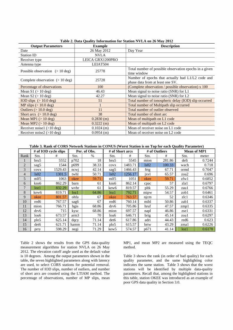
Table 2. Data Quality Information for Station NVLA on 26 May 2012
Output Parameters Example Description Date 26 May 2012 Day Year Station ID NVLA Receiver type LEICA GRX1200PRO Antenna type LEIAT504
Possible observation (> 10 deg) 25778 Total number of possible observation epochs in a given time window
Complete observation (> 10 deg) 25728 Number of epochs that actually had L1/L2 code and phase data from at least one SV.
Percentage of observations 100 (Complete observation / possible observation) x 100 Mean S1 (> 10 deg) 46.43 Mean signal to noise ratio (SNR) for L1 Mean S2 (> 10 deg) 42.27 Mean signal to noise ratio (SNR) for L2 IOD slips (> 10.0 deg) 51 Total number of ionospheric delay (IOD) slip occurred MP slips (> 10.0 deg) 1 Total number of Multipath slip occurred Outliers (> 10.0 deg) 11 Total number of outlier observed Short arcs (> 10.0 deg) 38 Total number of short arc Mean MP1 (> 10 deg) 0.2830 (m) Mean of multipath on L1 code Mean MP2 (> 10 deg) 0.3222 (m) Mean of multipath on L2 code Receiver noise1 (>10 deg) 0.1024 (m) Mean of receiver noise on L1 code Receiver noise2 (>10 deg) 0.0954 (m) Mean of receiver noise on L2 code
Table 3. Rank of CORS Network Stations in CONUS (Worst Station is on Top for each Quality Parameter) # of IOD cycle slips Per. of Obs. # of Short arcs # of Outliers Mean of MP1
Table 2 shows the results from the GPS data-quality measurement algorithms for station NVLA on 26 May 2012. The elevation cutoff angle used as the default value is 10 degrees. Among the output parameters shown in the table, the seven highlighted parameters along with latency are used, to select CORS stations for potential removal. The number of IOD slips, number of outliers, and number of short arcs are counted using the LTIAM method. The percentage of observations, number of MP slips, mean
MP1, and mean MP2 are measured using the TEQC method. Table 3 shows the rank (in order of bad quality) for each quality parameter, and the same highlighting color indicates the same station. Table 3 shows that the worst stations will be identified by multiple data-quality parameters. Recall that, among the highlighted stations in this table, station OKEE was introduced as an example of poor GPS data quality in Section 3.0.
Figure 7. Quality parameters measured at each station per day: a) number of IOD cycle slips (mean value over all 7
days and all stations is 37.98); b) number of short arcs (mean value over all 7 days and all stations is 32.74); c) number of outliers (mean value over all 7 days and all stations is 3.14); d) number of MP slips (mean value over all 7 days and
all stations is 13.24); e) mean of MP1 (average of mean MP1 over all 7 days and all stations is 0.2457 m); f) mean of MP2 (average of mean MP2 over all 7 days and all stations is 0.2826 m); g) percentage of observations (mean value
over all 7 days and all stations is 97.19%); and h) latency of each daily file for 7 days
0 500 1000 15000
2000
4000
6000
Num
ber o
f IO
D s
lip
Mean of all seven days on each stationsMinimum among seven days on each station
0 500 1000 15000
2000
4000
6000
Num
ber o
f Sho
rt ar
c
0 500 1000 15000
100
200
300
Num
ber o
f Out
lier
0 500 1000 15000
500
1000
1500
Num
ber o
f MP
slip
0 500 1000 15000
0.2
0.4
0.6
0.8
Mea
n of
MP
1 (m
)
0 500 1000 15000
0.2
0.4
0.6
0.8
Mea
n of
MP
2 (m
)
0 500 1000 15000
20
40
60
80
100
Station ID
Per
. of O
bs. (
%)
Maximum among seven days on each station0 500 1000 1500
0
2
4
6
Station ID
Late
ncy
of e
ach
daily
file
g) h)
e) f )
d)c)
a) b)
Figure 8. Probability density function of data-quality parameters for each station per day (data collected for 7 days):
a) number of IOD cycle slips; b) number of short arcs; c) number of outliers; d) number of MP slips; e) mean of MP1; f) mean of MP2; g) percentage of observations; and h) latency
0 2000 4000 6000 8000 10000-5
-4
-3
-2
-1
0
Number of IOD cycle slip
log 10
PD
F
0 2000 4000 6000 8000 10000-5
-4
-3
-2
-1
0
Number of Short arc
log 10
PD
F
0 100 200 300 400-5
-4
-3
-2
-1
0
Number of Outlier
log 10
PD
F
0 500 1000 1500-5
-4
-3
-2
-1
0
Number of MP slip
log 10
PD
F
0 0.2 0.4 0.6 0.8-5
-4
-3
-2
-1
0
Mean of MP1 (m)
log 10
PD
F
0 0.2 0.4 0.6 0.8 1-5
-4
-3
-2
-1
0
Mean of MP2 (m)
log 10
PD
F
0 20 40 60 80 100-5
-4
-3
-2
-1
0
Percentage of Observation (%)
log 10
PD
F
0 1 2 3 4 5 6-3
-2
-1
0
Latency
log 10
PD
F
+ 9
a) b)
c) d)
e) f )
g) h)
The results of analyzing the quality parameters of the CORS stations in CONUS show us how widely station performance can vary. Figure 7a shows the total number of IOD cycle slips counted over all satellites during 24 hours at each station. The station ID is plotted along the x-axis, and the number of IOD slips is plotted along the y-axis. These numbers are counted for the seven consecutive days shown in Table 1. The mean value (blue) and the minimum value (red) over seven days are close together for most stations, indicating that poor station quality persists for an extended period. From this test, 1.2 percent of stations had more than 500 IOD cycle slips per day, and more than 12 percent of stations had more than 50 IOD slips. Note that the mean value over all seven days and all stations is 37.98. As can be seen from Figures 7a to Figure 7h, the range of good and poor performance varies noticeably for each quality parameter. It can be observed that most stations maintain similar performance for the duration of this data set. Once station data quality is measured, detection thresholds for each quality parameter are set in order to remove poor stations. Figures 8a through 8h show the probability density function (PDF) of each quality parameter on each station per day in logarithmic scale. These test statistics are obtained from data collected for the seven days in Table 1. As an example, the PDF of the number of IOD cycle slips on each station per day is shown in Figure 8a. The red vertical lines in Figure 8 refer to the value of 9 (the mean value plus 9 times
the sample standard deviation) for each parameter. In Figures 8a – 8d, data (blue) exists continuously from 0 to this line, and the continuity of data ceases beyond this line. Thus, data that goes beyond 9 are considered to be
extreme outliers and are discarded from the distribution. For the mean of MP1 and the mean of MP2, no data exists beyond 9 .
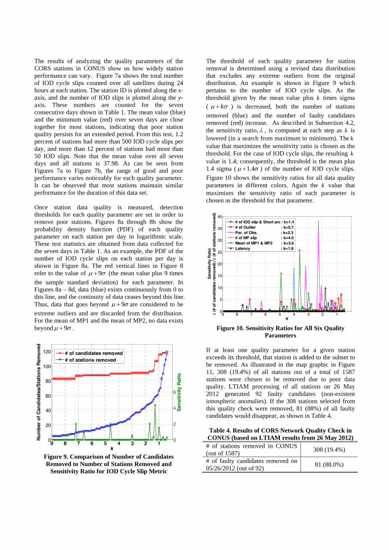
Figure 9. Comparison of Number of Candidates Removed to Number of Stations Removed and
Sensitivity Ratio for IOD Cycle Slip Metric
The threshold of each quality parameter for station removal is determined using a revised data distribution that excludes any extreme outliers from the original distribution. An example is shown in Figure 9 which pertains to the number of IOD cycle slips. As the threshold given by the mean value plus k times sigma ( k ) is decreased, both the number of stations
removed (blue) and the number of faulty candidates removed (red) increase. As described in Subsection 4.2, the sensitivity ratio, , is computed at each step as k is lowered (in a search from maximum to minimum). The k value that maximizes the sensitivity ratio is chosen as the threshold. For the case of IOD cycle slips, the resulting k value is 1.4; consequently, the threshold is the mean plus 1.4 sigma ( 1.4 ) of the number of IOD cycle slips.
Figure 10 shows the sensitivity ratios for all data quality parameters in different colors. Again the k value that maximizes the sensitivity ratio of each parameter is chosen as the threshold for that parameter.
Figure 10. Sensitivity Ratios for All Six Quality
Parameters If at least one quality parameter for a given station exceeds its threshold, that station is added to the subset to be removed. As illustrated in the map graphic in Figure 11, 308 (19.4%) of all stations out of a total of 1587 stations were chosen to be removed due to poor data quality. LTIAM processing of all stations on 26 May 2012 generated 92 faulty candidates (non-existent ionospheric anomalies). If the 308 stations selected from this quality check were removed, 81 (88%) of all faulty candidates would disappear, as shown in Table 4. Table 4. Results of CORS Network Quality Check in
CONUS (based on LTIAM results from 26 May 2012) # of stations removed in CONUS (out of 1587)
308 (19.4%)
# of faulty candidates removed on 05/26/2012 (out of 92)
81 (88.0%)
9 8 7 6 5 4 3 2 10
20
40
60
80
100
120
k
Nu
mb
er o
f C
and
idat
es/S
tati
on
s R
emo
ved
9 8 7 6 5 4 3 2 10
2
4
6
Sen
siti
vity
Rat
io
# of candidates removed# of stations removed
9 8 7 6 5 4 3 2 10
5
10
15
20
25
30
35
40
K
Sen
sitiv
ity R
atio
(#
of c
andi
date
s re
mov
ed) /
(#
of s
tatio
ns r
emov
ed)
# of IOD slip & Short arc : k=1.4# of Outlier : k=0.7Per. of Obs. : k=2.3# of MP slip : k=4.0Mean of MP1 & MP2 : k=3.6Latency : k=1.8
Figure 11. Map of CORS Network in CONUS
(Stations to be Removed in Red; Others in Blue)
Figure 12. Loss of Coverage (Red) due to Stations
Removed Figure 12 shows the station coverage CONUS when 308 stations are removed. Some stations, if removed, significantly reduce coverage (and ionospheric observability) in certain areas. As explained in Section 4.3, stations that significantly increase geographical observability are retained despite poor data quality. Station PRRY, shown in Figure 13, is one of the stations that are restored as a result of the geometry check. The region colored in dark gray is the station coverage formed by PRRY and two nearby stations (blue dots inside the green circle). Figure 13 shows the difference in station coverage before and after the removal of PRRY. In the case of PRRY, the loss of coverage (the change of the dark gray area) after the removal of PRRY is approximately 80%. Figure 14 shows the loss of coverage (red) that occurs when the PRRY station is removed. While PRRY is an unusual case, we have applied the rule that if the loss of coverage from station removal is above 30%, that station is determined to be a geographically critical station and is not removed. We performed the geometry check on the 308 stations which were classified as bad stations initially. Among these stations, 56 stations were deemed to be "geographically critical" stations and were not removed. These 56 stations are shown in green in Figure 15.
Figure 13. Comparison of Station Coverage before and
after Removal of Station PRRY
Figure 14. Loss of Coverage (Red) after Removing
Station PRRY
Figure 15. Map of CORS Stations in CONUS (Stations
Removed in Red; Stations Restored in Green)
Table 5. Results of Geometry Check on Stations Classified as “Poor Quality” (based on LTIAM results
from 26 May 2012) Before the
geometry check
After the geometry check
# of stations removed in CONUS (out of 1587)
308 (19.4%)
252 (15.9%)
# of faulty candidates removed on 05/26/2012 (out of 92)
81 (88.0%)
81 (88.0%)
Table 5 summarizes the results from the geometry check. After restoring these 56 stations, the number of faulty
120 oW
105oW 90oW
75oW
60o W
24 oN
36 oN
42oN
48oN
Longitude (deg)
Lat
itu
de
(deg
)
CORS Stations in CONUS
30oN
120 oW 105o
W 90oW 75oW
60o W
24 oN
30 oN
36 oN
42 oN
48 oN
Longitude (deg)
Lat
itu
de
(deg
)
CORS Stations in CONUS
ionospheric anomaly candidates removed stays the same compared to the results before the geometry check. The data-quality check and geometry check removed 88% of the total false anomalies while discarding only about 16% of the total stations. While this result is limited to the days in CONUS that were analyzed, it is important because it indicates that stations with "marginal" data quality can be retained where necessary for geographic observability without significantly increasing the number of faulty outputs from LTIAM. 6.0. UPDATED THREAT ANALYSIS FROM PAST
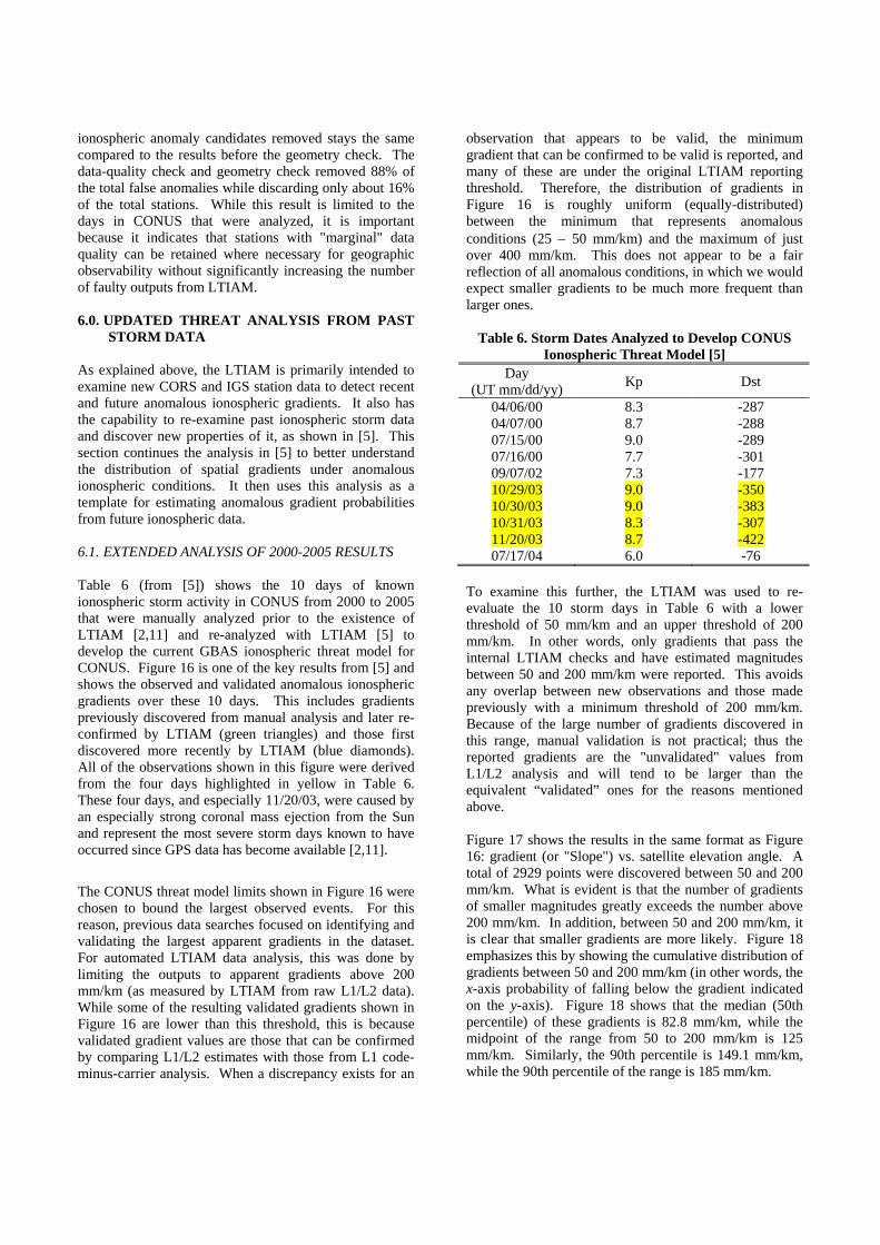
STORM DATA As explained above, the LTIAM is primarily intended to examine new CORS and IGS station data to detect recent and future anomalous ionospheric gradients. It also has the capability to re-examine past ionospheric storm data and discover new properties of it, as shown in [5]. This section continues the analysis in [5] to better understand the distribution of spatial gradients under anomalous ionospheric conditions. It then uses this analysis as a template for estimating anomalous gradient probabilities from future ionospheric data. 6.1. EXTENDED ANALYSIS OF 2000-2005 RESULTS Table 6 (from [5]) shows the 10 days of known ionospheric storm activity in CONUS from 2000 to 2005 that were manually analyzed prior to the existence of LTIAM [2,11] and re-analyzed with LTIAM [5] to develop the current GBAS ionospheric threat model for CONUS. Figure 16 is one of the key results from [5] and shows the observed and validated anomalous ionospheric gradients over these 10 days. This includes gradients previously discovered from manual analysis and later re-confirmed by LTIAM (green triangles) and those first discovered more recently by LTIAM (blue diamonds). All of the observations shown in this figure were derived from the four days highlighted in yellow in Table 6. These four days, and especially 11/20/03, were caused by an especially strong coronal mass ejection from the Sun and represent the most severe storm days known to have occurred since GPS data has become available [2,11].
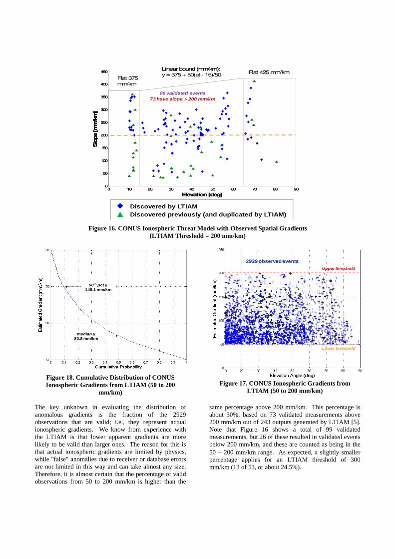
The CONUS threat model limits shown in Figure 16 were chosen to bound the largest observed events. For this reason, previous data searches focused on identifying and validating the largest apparent gradients in the dataset. For automated LTIAM data analysis, this was done by limiting the outputs to apparent gradients above 200 mm/km (as measured by LTIAM from raw L1/L2 data). While some of the resulting validated gradients shown in Figure 16 are lower than this threshold, this is because validated gradient values are those that can be confirmed by comparing L1/L2 estimates with those from L1 code-minus-carrier analysis. When a discrepancy exists for an
observation that appears to be valid, the minimum gradient that can be confirmed to be valid is reported, and many of these are under the original LTIAM reporting threshold. Therefore, the distribution of gradients in Figure 16 is roughly uniform (equally-distributed) between the minimum that represents anomalous conditions (25 50 mm/km) and the maximum of just over 400 mm/km. This does not appear to be a fair reflection of all anomalous conditions, in which we would expect smaller gradients to be much more frequent than larger ones.
To examine this further, the LTIAM was used to re-evaluate the 10 storm days in Table 6 with a lower threshold of 50 mm/km and an upper threshold of 200 mm/km. In other words, only gradients that pass the internal LTIAM checks and have estimated magnitudes between 50 and 200 mm/km were reported. This avoids any overlap between new observations and those made previously with a minimum threshold of 200 mm/km. Because of the large number of gradients discovered in this range, manual validation is not practical; thus the reported gradients are the "unvalidated" values from L1/L2 analysis and will tend to be larger than the equivalent “validated” ones for the reasons mentioned above. Figure 17 shows the results in the same format as Figure 16: gradient (or "Slope") vs. satellite elevation angle. A total of 2929 points were discovered between 50 and 200 mm/km. What is evident is that the number of gradients of smaller magnitudes greatly exceeds the number above 200 mm/km. In addition, between 50 and 200 mm/km, it is clear that smaller gradients are more likely. Figure 18 emphasizes this by showing the cumulative distribution of gradients between 50 and 200 mm/km (in other words, the x-axis probability of falling below the gradient indicated on the y-axis). Figure 18 shows that the median (50th percentile) of these gradients is 82.8 mm/km, while the midpoint of the range from 50 to 200 mm/km is 125 mm/km. Similarly, the 90th percentile is 149.1 mm/km, while the 90th percentile of the range is 185 mm/km.
Table 6. Storm Dates Analyzed to Develop CONUS Ionospheric Threat Model [5]
Figure 16. CONUS Ionospheric Threat Model with Observed Spatial Gradients (LTIAM Threshold = 200 mm/km)
Figure 18. Cumulative Distribution of CONUS Ionospheric Gradients from LTIAM (50 to 200
mm/km)
Figure 17. CONUS Ionospheric Gradients from
LTIAM (50 to 200 mm/km)
The key unknown in evaluating the distribution of anomalous gradients is the fraction of the 2929 observations that are valid; i.e., they represent actual ionospheric gradients. We know from experience with the LTIAM is that lower apparent gradients are more likely to be valid than larger ones. The reason for this is that actual ionospheric gradients are limited by physics, while "false" anomalies due to receiver or database errors are not limited in this way and can take almost any size. Therefore, it is almost certain that the percentage of valid observations from 50 to 200 mm/km is higher than the
same percentage above 200 mm/km. This percentage is about 30%, based on 73 validated measurements above 200 mm/km out of 243 outputs generated by LTIAM [5]. Note that Figure 16 shows a total of 99 validated measurements, but 26 of these resulted in validated events below 200 mm/km, and these are counted as being in the 50 200 mm/km range. As expected, a slightly smaller percentage applies for an LTIAM threshold of 300 mm/km (13 of 53, or about 24.5%).
Discovered by LTIAMDiscovered previously (and duplicated by LTIAM)
If we use 30% as a lower bound on the percentage of valid observations between 50 and 200 mm/km, the resulting estimate is 2929 × 0.3 = 878.7. Adding the 26 previously validated observations in this range gives a total of 904.7, or about 905 valid observations. The 73 validated observations above 200 mm/km thus represent a fraction of 73/(905+73), or about 7.5% of the total set of (estimated) validated observations. Above 300 mm/km, the ratio is 13/(905+73), or about 1.3% of the total set. If we instead assume as an upper bound that all 2929 measurements between 50 and 200 mm/km are valid, the ratio of validated observations above 200 mm/km would drop to 73/(2929+26+73), or about 2.4%, while the ratio above 300 mm/km would drop to 13/(2929+26+73) , or about 0.4%. These bounds show that, with very high confidence, the fraction of anomalous gradients above 200 mm/km in the 2000-2005 CONUS ionospheric storm data set is very small: below 10% at least, and very likely below 5%. Furthermore, since the distribution of LTIAM measurements between 50 and 200 mm/km is weighted toward the lower end, and lower gradients are more likely to be valid than higher ones, it is safe to conclude that the distribution of gradients throughout the CONUS threat space is heavily weighted toward the lower end of the gradient range. While GBAS ground stations must conservatively protect the entire threat space, including the highest possible gradients, this knowledge is not directly applicable to the ionospheric threat mitigations described in [1,12,13]. However, it helps us better understand ionospheric behavior relevant to GBAS during anomalous conditions, and it should lead to improved and less-conservative mitigation strategies in the future. 6.2. UPDATING PROBABILITY ESTIMATES WITH
FUTURE DATA The primary objective of LTIAM is to continually improve our understanding of both nominal and anomalous ionospheric gradient behavior. The re-analysis of past data in Section 6.1 shows an example of what can be learned. Going forward, the processing power of the LTIAM software allows automated analysis of all days in a particular region or a focus on particular days that appear anomalous based on external information such as ionospheric weather parameters [3,5]. The information collected over time from these results will allow us to update the probabilities estimated in Section 6.1 and gain a better idea of the "prior probability" of extreme ionospheric gradients (e.g., over 200 mm/km) (a) over all ionospheric conditions; and (b) conditional on the knowledge that anomalous conditions are present. It is important to distinguish these two results. If LTIAM processing of all data in a particular region is carried out, the distinction between "nominal" and "anomalous behavior" can be determined after the fact based on both
the observed gradients and external space weather information. In this case, probability estimates under all conditions and under anomalous conditions can be computed separately. If LTIAM processing is only carried out for days thought to be anomalous based on external information, only the latter estimate can be made. Updating the results in Section 6.1 is mostly a process of repeating the same analysis procedure with future data while including data already analyzed from the past. The desired result is a data-driven distribution of anomalous gradients, meaning gradients above 25 or 50 mm/km. The lower number represents the lower limit of the anomalous gradient space in the CONUS threat model, but gradients at this level are not threatening to GBAS. Therefore, it may be more practical to limit LTIAM searches to 50 mm/km or more, as done in this paper. While anomalous gradients of any magnitude are rare, continual monitoring will occasionally discover them and allow new points to be added to the observations made to date. Thus, our knowledge of the distribution of anomalous gradients will grow slowly with time. The rarity of severely anomalous gradients makes estimating their prior probability difficult. The model proposed in [14] uses the information available in early 2006 to estimate the probability of days with extremely anomalous ionospheric behavior, defined as days with gradients above 200 mm/km that could threaten GBAS (as shown in Table 6, all such days in the 2000-2005 database had Kp indices greater than 8.0). This probability was estimated as a mean of 0.00196 and a 60th percentile upper bound of 0.00257. The ability of LTIAM to process all days (or at least all days with significant ionospheric activity) allows us to improve upon the precision and usefulness of these numbers. Given a set of days analyzed (either “all days” or “days of significant activity”), the first probability to be computed is the fraction of days with any anomalous gradients, defined as either above 25 or above 50 mm/km. Combining this result with the distribution of gradients above 25 or 50 mm/km allows the computation of the probability of observing gradients above any particular magnitude (e.g., 200 mm/km) per unit time. While “days” was the time interval used in [14], LTIAM outputs can and should be grouped into smaller intervals, likely “hours,” to better reflect changing ionospheric conditions over the 24-hour “daily” cycle as well as the relatively short duration of anomalous gradients affecting particular areas. 7.0. SUMMARY This paper provides an overview of the LTIAM software processing tool and demonstrates how it is used to identify potential ionospheric spatial anomalies from raw
data collected by existing networks of CORS and IGS stations. Although LTIAM does its own screening of the raw data, significant ionospheric anomalies are rare; thus most of the results from LTIAM are "false" anomalies created by receiver or database errors. The vast majority of "false" anomalies come from relatively small subsets of CORS and IGS stations with poor data quality. The data quality evaluation methodology developed in this paper successfully reduced the number of false anomalies by almost 90% by removing only 16% of the CORS stations in CONUS. This was achieved while retaining stations with marginal data quality in geographically key locations. The end result is that the number of outputs requiring manual validation is greatly reduced. This paper also re-examines the database of known ionospheric storm events in CONUS from 2000 to 2005 to estimate the distribution of anomalous gradient magnitudes. Examining all gradients estimated to be greater than 50 mm/km by the LTIAM shows that the validated events with gradients above 200 mm/km are greatly outnumbered by events with gradients from 50 to 100 mm/km. The degree to which gradients above 200 mm/km are unusual depends upon the percentage of valid events from 50 to 200 mm/km, which is almost certainly larger than the approximately 30% that applies to anomalies above 200 mm/km in the same dataset. A simplified method is proposed to update this probability and estimate the overall probability of anomalous ionospheric conditions as more data is collected over time. ACKNOWLEDGMENTS The authors thank John Warburton of the FAA William J. Hughes Technical Center and his team for their support. We also would like to thank Jason Burns of the FAA, Oliver Jeannot, Cedric Lewis, Dieter Guenter, and Achanta Raghavendra of the AMT Tetra Tech, and Per Enge, Todd Walter, and Juan Blanch of Stanford for their support of this work. Minchan Kim was supported by Basic Science Research Program through the National Research Foundation of Korea (NRF) funded by the Ministry of Education, Science and Technology (2012-0007550). REFERENCES [1] Lee, J, Pullen, S, Datta-Barua, S, and Enge, P,
“Assessment of Ionosphere Spatial Decorrelation for Global Positioning System-Based Aircraft Landing System,” AIAA Journal of Aircraft, Vol. 44, No. 5, 2007, pp. 1662-1669.
[2] Datta-Barua, S., Lee, J., Pullen, S., Luo, M., Ene, A., Qiu, D., Zhang G., and Enge, P., “Ionospheric Threat Parameterization for Local Area GPS-Based Aircraft Landing Systems,” AIAA Journal of Aircraft, Vol. 47, No. 4, 2010, pp. 1141-1151.
[3] Lee, J., Jung, S., Bang, E., Pullen, S., and Enge, P., “Long Term Monitoring of Ionospheric Anomalies to Support the Local Area Augmentation System,” Proceedings of ION GNSS 2010, Portland, OR, Sept. 21-24, 2010, pp. 2651-2660.
[4] Lee, J., Jung, S., and Pullen, S., “Enhancements of Long Term Ionospheric Anomaly Monitoring for the Ground-Based Augmentation System,” Proceedings of ION ITM 2011, San Diego, CA, Jan. 24-26, 2011, pp. 930-941.
[5] Lee, J., Jung, S., Kim, M., Seo, J., Pullen, S., and Close, S., "Results from Automated Ionospheric Data Analysis for Ground-Based Augmentation Systems (GBAS)," Proceedings of ION NTM 2012, Newport Beach, CA, January 2012, pp. 1451-1461.
[6] Komjathy, A., Sparks, L, and Mannucci, A. J., “A New Algorithm for Generating High Precision Ionospheric Ground-Truth Measurements for FAA's Wide Area Augmentation System,” Jet Propulsion Laboratory, JPL Supertruth Document, Vol. 1, Pasadena, LA, July 2004.
[7] Jung. S and Lee, J. “Long-term ionospheric anomaly monitoring for ground based augmentation systems”, Radio science, 47, RS4006, doi:10.1029/2012RS005016.
[8] Estey, L. H. and Meertens, C. M., “TEQC: The Multi-Purpose Toolkit for GPS/GLONASS Data”, GPS solutions, Vol. 3, Issue 1, 1999, pp. 42-49
[10] Ge, L., Han, S., and Rizoz, C., “Multipath Mitigation of Continuous GPS Measurements Using an Adaptive Filter”, GPS solutions, Vol. 4, Issue 2, 2000, pp. 19-30.
[11] Lee, J., Datta-Barua, S., Zhang, G., Pullen, S., and Enge, P., “Observations of Low-Elevation Ionospheric Anomalies for Ground-Based Augmentation of GNSS,’ Radio Science, Vol. 46, 2011, RS6005.
[12] Lee, J., Seo, J., Park, Y. S., Pullen, S., and Enge, P., “Ionospheric Threat Mitigation by Geometry Screening in Ground-Based Augmentation Systems,” AIAA Journal of Aircraft, Vol. 48, No. 4, 2011, pp. 1422-1433.
[13] Seo, J., Lee, J., Pullen, S., Enge, P., and Close, S., “Targeted Parameter Inflation within Ground-Based Augmentation Systems to Minimize Anomalous Ionospheric Impact,” AIAA Journal of Aircraft, in press.
[14] Pullen, S., Rife, J., and Enge, P., "Prior Probability Model Development to Support System Safety Verification in the Presence of Anomalies," Proceedings of IEEE/ION PLANS 2006, San Diego, CA, April 25-27, 2006, pp. 1127-1136.