Data Rate Change Algorithms for HF Band Efficient ... · Sergeant 1st Class (OR-7) Mário Arede and...

Data Rate Change Algorithms for

HF Band Efficient Communications

Using the E/R GRC-525 Radio

Vasco Ferreira Sequeira

Thesis to obtain the Master of Science Degree in

Electrical and Computer Engineering

Supervisors

Prof. Maria Paula dos Santos Queluz Rodrigues

Prof. António José Castelo Branco Rodrigues

Prof. José Eduardo Charters Ribeiro da Cunha Sanguino

Maj Tm (Eng) Pedro Miguel Martins Grifo

Examination Committee

Chairperson: Prof. António Manuel Raminhos Cordeiro Grilo

Supervisor: Prof. Maria Paula dos Santos Queluz Rodrigues

Members of the Committee: Prof. Francisco António Bucho Cercas

TCor Tm (Eng) José Jaime Soares Pereira

November 2017

i

Acknowledgements

First, I would like to thank my family, they gave me all the values as a person and taught me to fight

for my goals, regardless of the obstacles that cross my path. To my father José Sequeira and my mother

Maria Teresa Sequeira, all my professional and personal successes are yours too. I would like to thank

also my girlfriend Verónica Rodriguez, who recently became an architect, for all the support, love and

patient she gave me, she motivated me to continue this stage successfully. All the words in the world

are few to describe how important you are to me.

A huge thank to the professors Paula Queluz, António Rodrigues and José Sanguino for accepting

since the first hour to supervise my thesis, with all the enthusiasm for this subject. All the support,

availability and transfer of knowledge resulted in a facilitated work. I expect that this partnership will be

an example for future researches, between the Instituto de Telecomunicações (IT) and the Portuguese

Armed Forces. Once again, I am very grateful for all the patient and dedication that the professors had

to help and guide my work.

Special thanks to Sistemas de Informação e Comunicação - Táctico (SIC-T) team project, led by

Major Pedro Grifo, who proposed the subject and gave me technical support to develop my master

dissertation with success, and all the knowledge about military communications equipment that I used

to achive the goals. I also want to thank the Sergeant 1st Class (OR-7) Francisco Pereira and the Staff

Sergeant (OR-6) Telmo Patricio, who gave me technical support to assembly and configure the

equipment. A huge thank to the remaining team Captain Tiago Guedes, Lieutenant Frederic Mota,

Sergeant 1st Class (OR-7) Mário Arede and Staff Sergeant (OR-6) Cristopher Monteiro, who welcomed

me and provided a good environment to work.

I want to thank to the Signals Regiment of Oporto, in special to the Signals Company from the

Intervention Brigade, led by Captain João Monteiro. Special thanks to the Staff Sergeant (OR-6) Luis

Pinto who gave me technical support to the field propagation tests and he coordinated the assembly of

the equipment in Oporto. These HF long distance communications proved that the Portuguese Army, in

special the Signals weapon, is an organization with competent staff interested in the communications

research and development; therefore, I want to pay tribute to all the officers, sergeants and soldiers who

collaborated in this master thesis research.

I want to thank my course of Military Academy, the Brigadeiro General D. Carlos Mascarenhas

course. It fills me with pride having shared with you all the difficulties and moments of comradeship that

taught me to value the little things of life. Special thanks for my comrades of the general course of

engineering who shared with me the same difficulties and helped me to get through it.

Lastly, I want to thank my Karaté-Do Portugal Shotokan family, which I have belonged for 20 years,

in special to my masters José Chagas and Cristina Amaral Mendes, who gave me all the moral and

behavioural formation, which is identified by the 5 karate maxims (Dojo Kun): character, sincerity, effort,

etiquette and self-control. To all my karate friends Joana Mendes, Monica Mendes, Diogo Cardoso and

João Fernandes thank you for sharing the good and the difficult moments, such as the friendship we

developed along these years.

ii

iii

Resumo

Desde os anos 80 que as comunicações na banda das altas frequências (HF) têm evoluído

tecnologicamente, sendo esta evolução motivada pela potencial robustez desta forma de comunicação

a situações de catástrofe e de emergência, e pelo custo de manutenção e implementação das

comunicações via satélite. Para o Exército Português, as comunicações em HF são também muito

importantes em Teatros de Operações com regiões montanhosas, como é o caso do Kosovo e do

Afeganistão, onde esta força representa Portugal em missões das Nações Unidas (ONU) ou da

Organização do Tratado do Atlântico Norte (NATO – North Atlantic Treaty Organization). Neste

contexto, são particularmente interessantes as comunicações em HF que utilizam ondas de rádio com

ângulos de incidência (na Ionosfera) próximos de zero graus, e designadas na literatura Inglesa por

Near Vertical Incidence Sky waves (NVIS). Apesar do renascimento no interesse das comunicações

em HF, existem vários desafios envolvidos, como a operação rádio com relações sinal-ruido (SNR)

tipicamente muito baixas, desvanecimento (fading), variação do sinal devido a mudanças na camada

da Ionosfera, e capacidade limitada do canal. Para lidar com as mudanças do canal em HF, surgiram

várias tecnologias como a análise automática da qualidade da ligação (LQA), o estabelecimento

automático da ligação (ALE) e a mudança automática do débito binário (DRC), eliminando a

necessidade de procedimentos operacionais complexos e manuais.

Motivado pelas soluções desenvolvidas ao longo dos anos, esta Dissertação começa com a visão

geral do estado-de-arte disponível na área dos algoritmos de Mudança de Débito Binário (DRC),

analisando as vulnerabilidades dos algoritmos existentes e propondo soluções para as melhorar. A

primeira proposta evita valores altos de taxa de erro de bit (BER) que conduzem a um estado de corte

da ligação; a segunda proposta, para além de aumentar a disponibilidade da ligação, também evita

oscilações desnecessárias do débito binário. Quando testadas no ambiente de simulação, ambas as

propostas mostraram melhores desempenhos que os algoritmos originais. Esta melhoria de

desempenho também foi confirmada em condições reais de transmissão, depois de implementar os

algoritmos no rádio E/R GRC-525, e de estabelecer uma comunicação HF entre duas estações

localizadas em Lisboa e Porto, usando a antena dipolo RF-1936P. Nos testes de propagação no terreno

a melhor proposta permite um aumento de 15% na disponibilidade da ligação e de 392% na taxa média

de tramas corretas recebidas (goodput), em comparação com o algoritmo original.

Palavras-chave: Algoritmo de Seleção de Débito Binário (DRC), Comunicações em HF, Ionosfera,

Relação Sinal-Ruído (SNR), Taxa de Erro de Bit (BER).

iv

v

Abstract

Since the 80s that communications on the high frequency (HF) band have undergone a remarkable

technologic evolution, motivated by their potential robustness to catastrophic and emergency situations,

and by the high costs involved on the implementation and maintenance of satellite links. For the

Portuguese Army, the HF communications are also very important in Theatre of Operations with

mountainous regions, like Kosovo and Afghanistan, where this force represents Portugal in United

Nations (UN) and North Atlantic Treaty Organization (NATO) missions. In this context, HF

communications using radio waves with incidence angles (in Ionosphere) near zero degrees - known as

Near Vertical Incidence Sky waves (NVIS) - are often used. Despite the renewed interest on HF

communications, there are a lot of challenges involved, like the operation with (typically) very low signal-

to-noise ratios (SNR), multipath fading, signal variation due to the changing constitution of the

ionosphere, and a limited channel capacity. In order to deal with the variability of the HF channel, several

technologies have emerged, like automatic Link Quality Analysis (LQA), Automatic Link Establishment

(ALE) and automatic Data Rate Change (DRC), eliminating the need for complex and manual operating

procedures.

Motivated by the developed solutions along the last years for DRC algorithms, this Dissertation starts

with an overview of the available state-of-the-art, to assess the vulnerabilities of existing algorithms and

propose solutions to overcome them. The first proposal avoids high Bit Error Rate (BER) values that

lead to a link cut-off state (i.e., disconnection); the second proposal, besides increasing the link

availability, also avoids unnecessary data rate oscillations. When assessed on a simulation

environment, both proposals showed better performance than the original algorithms. This performance

improvement was also confirmed in real transmission conditions, after implementing the algorithms on

the E/R GRC-525 radio, and establishing a HF connection between two communication stations located

in Lisbon and Oporto, using the RF-1936P dipole antenna. In the field propagation tests, the best

proposal allows an increase of 15% on the link availability and of 392% on the average goodput,

relatively to the original algorithm.

Key-words: Bit Error Rate (BER), Data Rate Change (DRC) Algorithm, High Frequency (HF)

Communications, Ionosphere, Signal-to-Noise Ratio (SNR).

vi

vii

Table of Contents

Acknowledgements ......................................................................................................................... i

Resumo ........................................................................................................................................ iii

Abstract ......................................................................................................................................... v

List of Figures ............................................................................................................................... xi

List of Tables ............................................................................................................................. xvii

List of Acronyms ......................................................................................................................... xix

Chapter 1 - Introduction .................................................................................................................1

1.1. Context and Motivation ........................................................................................................1

1.2. Objectives ...........................................................................................................................3

1.3. Main Contributions ..............................................................................................................3

1.4. Dissertation Structure ..........................................................................................................3

Chapter 2 - HF Communications ....................................................................................................5

2.1. Types of HF Radio Signals ..................................................................................................5

2.2. Propagation by the Ionosphere ............................................................................................6

2.2.1. The Ionosphere Layer ...................................................................................................6

2.2.2. Near-Vertical Incidence Sky wave .................................................................................9

2.3. HF Antennas ..................................................................................................................... 10

Chapter 3 - HF Communication Standards ................................................................................... 13

3.1. Adaptive Techniques in HF Communications ..................................................................... 13

3.2. Overview of HF Communications Standards ...................................................................... 14

3.3. Physical Layer ................................................................................................................... 15

3.4. Automatic Channel Selection (ACS) .................................................................................. 18

3.5. Automatic Link Establishment (ALE) .................................................................................. 18

3.6. Automatic Link Maintenance (ALM) ................................................................................... 19

3.7. Data Link Protocol ............................................................................................................. 20

3.7.1. High Throughput Data Link ......................................................................................... 20

3.7.2. Low Latency Data Link................................................................................................ 20

3.7.3. High Throughput Data Link+ ....................................................................................... 20

Chapter 4 - State-of-the-art on Data Rate Change Algorithms ...................................................... 23

viii

4.1. DRC algorithm for non-Autobaud Modulations ................................................................... 23

4.2. DRC algorithm for Autobaud Modulations .......................................................................... 24

4.3. RapidM DRC algorithm ..................................................................................................... 25

4.3.1. RapidM DRC algorithm 1 design ................................................................................. 26

4.3.2. RapidM DRC algorithm 1 implementation .................................................................... 29

4.3.3. RapidM DRC algorithm 1 simulation, results and tests ................................................ 30

Chapter 5 – DRC Algorithm: Assessment of Existing Solutions and Proposals for Improvement ... 33

5.1. DRC Algorithms Simulation System ................................................................................... 33

5.2. Previous DRC algorithms: Simulation and Assessment ...................................................... 37

5.2.1. Trinder algorithm Simulation and Assessment ............................................................. 37

5.2.2. RapidM DRC algorithm Simulation and Assessment ................................................... 39

5.3. Improvements on the Trinder and RapidM Algorithms ........................................................ 41

5.3.1. Avoiding Cut-Off State Algorithm ................................................................................ 41

5.3.2. Bit Error Optimization Algorithm .................................................................................. 46

5.4. Conclusion ........................................................................................................................ 51

Chapter 6 – Field Propagation Tests ............................................................................................ 53

6.1. Equipment Assembly and Configuration Procedures .......................................................... 53

6.1.1. General Settings and Components ............................................................................. 54

6.1.2. Assembly of Bench Tests Circuit ................................................................................. 58

6.1.3. Assembly of Field Tests Equipment ............................................................................ 59

6.2. Data Rate Change Software Application ............................................................................ 60

6.2.1. User Application Configuration .................................................................................... 60

6.2.2. Output Files and Graphical Views ............................................................................... 62

6.3. Field Propagation Tests: Environment Conditions and Results ........................................... 63

6.3.1. Meteorological and Ionospheric Conditions for Test Days ........................................... 64

6.3.2. Algorithms Performance in Real Test Conditions ......................................................... 64

6.4. Relation between Simulations and Field Propagation Values ............................................. 68

Chapter 7 – Summary and Future Work ....................................................................................... 73

7.1. Summary........................................................................................................................... 73

7.2. Future Work ...................................................................................................................... 74

Appendix A – Radio E/R GRC-525 datasheet ............................................................................... 75

ix

Appendix B – Dipole antenna RF-1936P datasheet ...................................................................... 77

Appendix C – Results from Algorithms Assessments .................................................................... 79

Appendix D – HF Communications Electrical Message ................................................................. 87

Appendix E – Assembly of the Dipole Antenna 1936P .................................................................. 89

Appendix F – Results from the Field Propagation Tests ................................................................ 91

Appendix G – Ionospheric Conditions for the Test Days ............................................................. 111

Bibliography ............................................................................................................................... 113

x

xi

List of Figures

Figure 1.1 - Example of HF channel propagation waves [1]. ................................................................1

Figure 1.2 – Image of the E/R GRC-525 [2]. ........................................................................................2

Figure 2.1 – Radio Spectrum [8]. .........................................................................................................5

Figure 2.2 – The Ionosphere Layers [10]. ............................................................................................6

Figure 2.3 – Ionosphere behaviour: a) reflection depending on the frequency; b) reflection depending

on the day time [13]. ...........................................................................................................................7

Figure 2.4– Reflection of type M [14]. ..................................................................................................7

Figure 2.5 – Reflection of type N [14]. .................................................................................................7

Figure 2.6 - Example of an Ionogram: a) real [16]; b) schematic. .........................................................8

Figure 2.7 – Example of a Global Real Time Ionospheric foF2 Map [17]. .............................................8

Figure 2.8 – NVIS propagation and its characteristic "umbrella" shape [19]. ........................................9

Figure 2.9 – Change of the critical frequency during the day, and on winter [16]. ............................... 10

Figure 2.10 – Antennas used in NVIS: a) horizontal dipole antenna [15]; b) circular loop antenna [21].

......................................................................................................................................................... 11

Figure 2.11 – Gain of three different antennas used in NVIS propagation [16]. .................................. 11

Figure 2.12 – Use of the Whip antenna for NVIS communication [16]. ............................................... 12

Figure 3.1 – ARCS process cycle [18]. .............................................................................................. 14

Figure 3.2 – The HF house of standards [18]. .................................................................................... 15

Figure 3.3 – Frame structure for all modulations [24]. ........................................................................ 16

Figure 3.4 – Synchronous dwell structure in 3rd Generation ALE [22]. ................................................ 18

Figure 3.5 – The 3rd Generation ALE call [22]. ................................................................................... 19

Figure 3.6 - HDL+ Header [29]. ......................................................................................................... 21

Figure 4.1 – ARQ throughput as a function of SNR [6]. ...................................................................... 24

Figure 4.2 – RapidM DRC algorithm1 system of inputs and outputs [3]. ............................................. 26

Figure 4.3 – RapidM DRC Algorithm1 flowchart (Adapted from [3]). ................................................... 27

Figure 4.4 – The fitted line through the 10 − 5 BER points [3]. ........................................................... 28

Figure 4.5 – Input and Output system of the RapidM DRC algorithm 1 implementation (Adapted from

[3]). ................................................................................................................................................... 29

Figure 4.6 – BER channel profile [3]. ................................................................................................. 30

Figure 5.1 – Simulation system flowchart. ......................................................................................... 33

Figure 5.2 – BER as a function of SNR for m-QAM modulation, with a straight line (in green) representing

a BER variation of 1 decade per dB (Adapted from [32]). ................................................................... 34

Figure 5.3 – Channel measurements time diagram. ........................................................................... 34

Figure 5.4 – Downward sinusoidal SNR variation. ............................................................................. 36

Figure 5.5 – Upward sinusoidal SNR variation. .................................................................................. 36

Figure 5.6 – Sinusoidal SNR variation. .............................................................................................. 36

Figure 5.7 – Step-wise SNR variation. ............................................................................................... 36

Figure 5.8 – Trinder algorithm data rate variation, for an upward sinusoidal SNR variation. ............... 38

xii

Figure 5.9 – Trinder algorithm: BER vs Data Rate variation, for an upward sinusoidal SNR variation

using an ITU Poor channel. ............................................................................................................... 39

Figure 5.10 – Original RapidM algorithm data rate variation, for an upward sinusoidal SNR variation. 40

Figure 5.11 – RapidM DRC algorithm: BER vs Data Rate variation, for an upward sinusoidal SNR

variation using an ITU Poor channel. ................................................................................................. 40

Figure 5.12 – Avoiding Cut-Off State algorithm flowchart. .................................................................. 42

Figure 5.13 – Trinder algorithm with ACOS data rate variation, for an upward sinusoidal SNR variation.

......................................................................................................................................................... 42

Figure 5.14 – Trinder algorithm with ACOS: BER vs Data Rate variation, for an upward sinusoidal SNR


Figure 5.15 – RapidM algorithm with ACOS data rate variation, for an upward sinusoidal SNR variation.

......................................................................................................................................................... 45

Figure 5.16 – RapidM DRC algorithm with ACOS: BER vs Data Rate variation, for an upward sinusoidal

SNR variation using an ITU Poor channel. ........................................................................................ 46

Figure 5.17 – Bit Error Optimization algorithm flowchart. ................................................................... 46

Figure 5.18 – Trinder algorithm with BEO data rate variation, for an upward sinusoidal SNR variation.

......................................................................................................................................................... 47

Figure 5.19 – Trinder algorithm with BEO: BER vs Data Rate variation, for an upward sinusoidal SNR


Figure 5.20 – RapidM algorithm with BEO data rate variation, for an upward sinusoidal SNR variation.

......................................................................................................................................................... 49

Figure 5.21 – RapidM DRC algorithm with BEO: BER vs Data Rate variation, for an upward sinusoidal

SNR variation using an ITU Poor channel. ........................................................................................ 50

Figure 6.1 – Dipole antenna RF-1936P from Harris Corporation. ....................................................... 53

Figure 6.2 – Critical frequency of F2 layer in real time for the 28th of August 2017 (Consulted on [17]).

......................................................................................................................................................... 54

Figure 6.3 – Real time Ionospheric data for the 28th August 2017: a) MUF values in percentage during

the day (Consulted on [36]); b) Warnings that may influence the HF communications (Consulted on

[17]). ................................................................................................................................................. 55

Figure 6.4 – Process of downloading the mission on the radio: a) Fill Gun HQ produced by EID; b) Data

transfer from the Fill Gun HQ to the E/R GRC-525. ........................................................................... 55

Figure 6.5 – Wattmeter used to verify the reflected wave power of each frequency: a) Image of the

wattmeter produced by Bird Electronic Corporation; b) Practical use of the wattmeter. ...................... 56

Figure 6.6 – ATU learning process: a) ATU learning the group of eight available frequencies; b) Message

when the tuning is performed successfully. ....................................................................................... 56

Figure 6.7 – Hardware components used in the experiments: a) Assembly of a computer running the

DRC application on the radio; b) RS232/USB cable used as serial and data port, produced by EID; c)

Micro-headset from the E/R GRC-525 radio, produced by EID; d) Several meters of coaxial cable. ... 57

Figure 6.8 – Hardware components used specifically for bench experiments: a) Variable HF attenuator,

produced by EID; b) Fixed attenuator of 30 dB to assembly on the transmitter output. ....................... 58

xiii

Figure 6.9 – Schematic of the bench circuit used to test the DRC application. ................................... 58

Figure 6.10 – Physical assembly of the bench tests circuit: a) Output system with a TX station and the

fixed attenuator of 30 dB; b) Input system with the RX station and the variable HF attenuator. ........... 59

Figure 6.11 – Location of the HF stations: a) Station one located in Logistics Support Unity, Paço de

Arcos, Lisbon; b) Station two located in the Signals Regiment, Viso de Baixo, Oporto. ...................... 59

Figure 6.12 – Image of the two dipole antennas RF-1936P used to perform the field propagation tests:

a) Antenna located in the Signals Regiment, Viso de Baixo, Oporto; b) Antenna located in Logistics

Support Unity, Paço de Arcos, Lisbon. .............................................................................................. 60

Figure 6.13 – Output tab page of the DRC application. ...................................................................... 61

Figure 6.14 – Configuration tab page from the DRC application: a) Parameters to open the remote

control port and starting the channel sounding; b) Signal when the remote control is open: green light

when the remote control port is open and red light when it is closed; c) Fields to set the interleaver size.

......................................................................................................................................................... 61

Figure 6.15 – Algorithms tab page from the DRC application: a) Type of algorithm, type of channel and

number of version settings; b) Process to open the data send port. ................................................... 62

Figure 6.16 – Handling files in the DRC application: a) Create a file with a defined name and size; b)

Sending the created file. ................................................................................................................... 62

Figure 6.17 – DRC application graphical view with the interval of SNR measures and data rate settings.

......................................................................................................................................................... 63

Figure 6.18 – Data rate adaption for a SNR variation measured in 30th August 2017, using the original

DRC RapidM algorithm. .................................................................................................................... 65

Figure 6.19 – Data rate adaption for a SNR variation measured in 31st August 2017, using the DRC

RapidM algorithm with ACOS. ........................................................................................................... 66

Figure 6.20 – Data rate adaption for a SNR variation measured in 1st September 2017, using the DRC

RapidM algorithm with BEO. ............................................................................................................. 66

Figure 6.21 – Data rate adaption for a SNR variation measured in 4th September 2017, using the original

Trinder algorithm. .............................................................................................................................. 67

Figure 6.22 – Data rate adaption for a SNR variation measured in 5th September 2017, using the Trinder

algorithm with ACOS. ........................................................................................................................ 67

Figure 6.23 – Data rate adaption for a SNR variation measured in 7th September 2017, using the Trinder

algorithm with BEO. .......................................................................................................................... 68

Figure 6.24 – Cross-correlation coefficient values between the field propagation tests and the expected

results provided by the simulation system (graphic representation). ................................................... 69

Figure 6.25 – Simulated values for the 5th September 2017, using Trinder algorithm with ACOS and

assuming an AWGN channel which corresponds to the best cross-correlation fit. .............................. 70

Figure 6.26 – Simulated values for the 4th September 2017, using original Trinder algorithm and

assuming an AWGN channel which corresponds to the worst cross-correlation fit. ............................ 70

Figure C.1 – Trinder algorithm data rate adaptation for an AWGN channel using downward sinusoidal

SNR variation.................................................................................................................................... 79

xiv

Figure C.2 – Trinder algorithm data rate adaptation for a GOOD channel using downward sinusoidal

SNR variation.................................................................................................................................... 79

Figure C.3 - Trinder algorithm data rate adaptation for a POOR channel using downward sinusoidal

SNR variation.................................................................................................................................... 79

Figure C.4 – Trinder algorithm data rate adaptation for an AWGN channel using upward sinusoidal SNR

variation. ........................................................................................................................................... 80

Figure C.5 – Trinder algorithm data rate adaptation for a GOOD channel using upward sinusoidal SNR

variation. ........................................................................................................................................... 80

Figure C.6 – Trinder algorithm data rate adaptation for a POOR channel using upward sinusoidal SNR

variation. ........................................................................................................................................... 80

Figure C.7 – Trinder algorithm data rate adaptation for an AWGN channel using sinusoidal SNR

variation. ........................................................................................................................................... 81

Figure C.8 – Trinder algorithm data rate adaptation for a GOOD channel using sinusoidal SNR variation.

......................................................................................................................................................... 81

Figure C.9 – Trinder algorithm data rate adaptation for a POOR channel using sinusoidal SNR variation.

......................................................................................................................................................... 81

Figure C.10 – Trinder algorithm data rate adaptation for an AWGN channel using discontinues SNR

variation. ........................................................................................................................................... 82

Figure C.11 – Trinder algorithm data rate adaptation for a GOOD channel using discontinues SNR

variation. ........................................................................................................................................... 82

Figure C.12 – Trinder algorithm data rate adaptation for a POOR channel using discontinues SNR

variation. ........................................................................................................................................... 82

Figure C.13 – RapidM algorithm data rate adaptation for an AWGN channel using downward SNR

variation. ........................................................................................................................................... 83

Figure C.14 – RapidM algorithm data rate adaptation for a GOOD channel using downward SNR

variation. ........................................................................................................................................... 83

Figure C.15 – RapidM algorithm data rate adaptation for a POOR channel using downward SNR

variation. ........................................................................................................................................... 83

Figure C.16 – RapidM algorithm data rate adaptation for an AWGN channel using upward SNR variation.

......................................................................................................................................................... 84

Figure C.17 – RapidM algorithm data rate adaptation for a GOOD channel using upward SNR variation.

......................................................................................................................................................... 84

Figure C.18 – RapidM algorithm data rate adaptation for a POOR channel using upward SNR variation.

......................................................................................................................................................... 84

Figure C.19 – RapidM algorithm data rate adaptation for an AWGN channel using sinusoidal SNR

variation. ........................................................................................................................................... 85

Figure C.20 – RapidM algorithm data rate adaptation for a GOOD channel using sinusoidal SNR

variation. ........................................................................................................................................... 85

Figure C.21 – RapidM algorithm data rate adaptation for a POOR channel using sinusoidal SNR

variation. ........................................................................................................................................... 85

xv

Figure C.22 – RapidM algorithm data rate adaptation for an AWGN channel using discontinues SNR

variation. ........................................................................................................................................... 86

Figure C.23 – RapidM algorithm data rate adaptation for a GOOD channel using discontinues SNR

variation. ........................................................................................................................................... 86

Figure C.24 – RapidM algorithm data rate adaptation for a POOR channel using discontinues SNR

variation. ........................................................................................................................................... 86

Figure E.1 – Assembly of the station one images: a) Unroll the dipole wires; b) Attaching the copper bar

to perform the ground of the system; c) Wire that connect the radio with the antenna; d) Fixing the base

of the antenna to the ground; e) Hoist the mast of the antenna; f) Stretching the coaxial cable to the

radio station. ..................................................................................................................................... 89

Figure G.1 – Ionospheric conditions for the 30th August 2017: a) foF2 real measure in red colour, and

foF2 predicted value in white colour during the day; b) MUF values during the day. ......................... 111

Figure G.2 – Ionospheric conditions for the 31st August 2017: a) foF2 real measure in red colour, and


Figure G.3 – Ionospheric conditions for the 1st September 2017: a) foF2 real measure in red colour, and


Figure G.4 – Ionospheric conditions for the 4th September 2017: a) foF2 real measure in red colour, and


Figure G.5 – Ionospheric conditions for the 5th September 2017: a) foF2 real measure in red colour, and


Figure G.6– Ionospheric conditions for the 7th September 2017: a) foF2 real measure in red colour, and


xvi

xvii

List of Tables

Table 3.1 – Modulation used for each data rate (adapted from [24] and [25]). .................................... 16

Table 3.2 – SNR requirements for a BER of 10 − 5 using an AWGN channel (Adapted from [3]). .... 17

Table 3.3 – SNR requirements for a BER of 10 − 5 using an ITU Good channel (Adapted from [3]). 17

Table 3.4 – SNR requirements for a BER of 10 − 5 using an ITU Poor channel (Adapted from [3]). . 17

Table 4.1 – FER thresholder values used for DRC algorithm for Autobaud Modulations [6]. ............... 25

Table 4.2 – RapidM DRC algorithm 1 input parameters [3]. ............................................................... 26

Table 4.3 – Number of frames received after 127s interval and frame length of 250 bytes (Adapted from

[3]). ................................................................................................................................................... 26

Table 4.4 – BER decision thresholder for RapidM DRC algorithm 2 (Adapted from [3]). ..................... 28

Table 4.5 – Simulation constants (Adapted from [3]). ......................................................................... 31

Table 4.6 – Test settings for RapidM DRC algorithm 1 (Adapted from [3]). ........................................ 31

Table 4.7 – Results for data throughput test for Trinder and RapidM DRC algorithms (Adapted from [3]).

......................................................................................................................................................... 31

Table 4.8 – Results for acquisition time test for Trinder and RapidM DRC algorithms (Adapted from [3]).

......................................................................................................................................................... 32

Table 5.1 – Trinder algorithm simulation results for each channel type. ............................................. 38

Table 5.2 – RapidM DRC algorithm simulation results for each type of channel. ................................ 39

Table 5.3 – Relative variation between RapidM DRC and Trinder algorithm. ..................................... 41

Table 5.4 - Trinder algorithm with ACOS simulation results for each channel type. ............................ 43

Table 5.5 – Relative variation between Trinder with ACOS and original Trinder algorithm. ................. 43

Table 5.6 – RapidM DRC algorithm with ACOS simulation results for each channel type. .................. 44

Table 5.7 – Relative variation between RapidM DRC algorithm with ACOS and its original version. ... 45

Table 5.8 – Trinder algorithm with BEO simulation results for each channel type. .............................. 47

Table 5.9 – Relative variation between Trinder algorithm with BEO and the original version. ............. 48

Table 5.10 – RapidM DRC algorithm with BEO simulation results for each channel type.................... 49

Table 5.11 – Relative variation between RapidM DRC algorithm with BEO and the original version. .. 50

Table 6.1 – Meteorological conditions and Ionospheric warnings for test days. .................................. 64

Table 6.2 – Overall results of the field propagation tests. ................................................................... 64

Table 6.3 – Cross-correlation coefficients values between the field propagation tests results and the

excepted results provided by the simulation system. ......................................................................... 68

Table 6.4 – Relation between the field propagation results and the expected values for each channel

provided by the simulation system. .................................................................................................... 71

Table F.1 - Results from the Field Propagation Tests on 30th August 2017 using the DRC RapidM

algorithm. .......................................................................................................................................... 91

Table F.2 – Results from the Field Propagation Tests on 31st August 2017 using the DRC RapidM

algorithm with ACOS. ........................................................................................................................ 93

Table F.3 – Results from the Field Propagation Tests on 1st September 2017 using the DRC RapidM

algorithm with BEO. .......................................................................................................................... 97

xviii

Table F.4 – Results from the Field Propagation Tests on 4th September 2017 using the Trinder algorithm.

....................................................................................................................................................... 100

Table F.5 – Results from the Field Propagation Tests on 5th September 2017 using the Trinder algorithm

with ACOS. ..................................................................................................................................... 102

Table F.6 – Results from the Field Propagation Tests on 7th September 2017 using the Trinder algorithm

with BEO. ....................................................................................................................................... 107

xix

List of Acronyms

2G 2nd Generation

3G 3rd Generation

3G-ALE 3rd Generation Automatic Link Establishment

ACK Acknowledgement

ACO S Avoiding Cut-Off State

ACS Automatic Channel Selection

ALE Automatic Link Establishment

ALM Automatic Link Maintenance

ARCS Automatic Radio Control System

ARQ Automatic Repeat Request

ATU Antenna Tuning Unity

AWGN Additive White Gaussian Noise

BEO Bit Error Optimization

BER Bit Error Rate

BLOS Beyond Line-of-Sight

BW6 Burst Waveform 6

CM Connection Management

CRC Cyclic Redundancy Check

CSMA Carrier-Sense-Multiple-Access

DCSI Direção de Comunicações e Sistemas de Informação

DRC Data Rate Change

DTS Data Transfer Sub-layer

E/R GRC-525 Portuguese Military Radio

EID Empresa de Investigação e Desenvolvimento de Eletrónica

EPM Electronic Protection Measures

EW Electronic Warfare

FER Frame Error Rate

foF2 Critical Frequency of the F2 Layer

HDL High Throughput Data Link

HDL+ High Throughput Data Link+

HF High-Frequency

HFCS High Frequency Channel Simulator

IRE Institute of Radio Engineers

IRI International Reference Ionosphere

IT Instituto de Telecomunicações

ITU International Telecommunications Union

LDL Low Latency Data Link

LM Link Maintenance

LOS Line-of-Sight

xx

LQA Link Quality Analysis

LSU Link Setup

LUF Lowest Usable Frequency

MIL-STD United States Military Standard

MUF Maximum Usable Frequency

NATO North Atlantic Treaty Organization

NFO National Force Outstanding

NLOS Non-Line-Of-Sight

NVIS Near Vertical Incidence Sky wave

OSI Open Systems Interconnection

PDUs Protocol Data Units

PSK Phase Shift Keying

PU Participating Unit

RX Receiver

SIC-T Sistemas de Informação e Comunicação - Tático

SNMP Simple Network Management Protocol

SNR Signal-to-Noise Ratio

STANAG NATO Standardisation Agreement

TM Traffic Management

TO Theatre of Operations

TX Transmitter

UHF Ultra High-Frequency

UN United Nations

UV Ultraviolet

VHF Very High-Frequency

WRC-97 1997 World Radiocommunication Conference

1

1. Chapter 1 - Introduction

This chapter presents the motivation and the context of the problem to be solved; the main

characteristics of high frequency (HF) signals and the importance of these signals in military

communications are also described. Finally, the objectives, the main contributions and the structure of

the Master Dissertation are outlined.

1.1. Context and Motivation

HF communications have been used by military organizations since the end of the First World War.

These communications use the range of radio frequencies of the electromagnetic spectrum between 3

MHz and 30 MHz, known as HF band, allowing long distance transmissions (e.g., inter-continental)

without the need of repeaters.

Before the 60s, HF radio signals were the primary source of long-range communications; in the 60s

and 70s the HF transmissions declined because satellite communications allowed much higher data

rates. However, satellites are vulnerable to physical damage and it is expensive to build and maintain

them. In the beginning of the new millennium, the development of Automatic Link Establishment (ALE)

technologies, including automated frequency selection and high speed modems (up to 9600 bit/s) for

HF communications, have led to a renaissance in the HF usage.

HF frequencies are refracted by the Ionosphere, enabling beyond line-of-sight (BLOS)

communications; this atmosphere layer is a region of electrically charged particles and it is situated,

approximately, between 50 to 600 kilometres above the earth’s surface. This layer refracts the signal

back to earth several times, depending on the amount of ionization, before the signal reaches its

destination, acting like a natural satellite.

The HF signals propagate, generally, in two ways: ground waves and sky waves (Figure 1.1). The

ground waves can be direct, surface or ground reflected waves. Depending on the time of the day, of

the atmosphere conditions and on the operating frequencies, sky waves can be refracted returning to

the Earth surface hundreds or thousands of kilometres away, allowing long-range communications; this

dissertation considers mainly this type of waves.

Figure 1.1 – Example of HF channel propagation waves [1].

2

The sky waves with most interest for military operations are the Near Vertical Incidence Sky waves

(NVIS), which are characterized by having high tilt angles, typically between 60º and 89º. There are

several advantages in the use of the NVIS, like the possibility of communication over hilly terrain without

the need for repeaters; additionally, this form of propagation needs only one operator in the field using

a small antenna, like a simple dipole antenna, which is very practical for military operations. For these

reasons, the NVIS communication in HF band is often used in emergency situations and in the Theatre

of Operations (TO).

The Portuguese Army participates in several National Force Outstanding (NFO), and the most

common NFOs locations are situated in hilly terrain, like those in Afghanistan and Kosovo. The NVIS

communications are used in NFO since 1996, in the Bosnia and Herzegovina’s mission, and supported

mainly by the military radio E/R GRC-525. This radio was developed by the Portuguese Army and by

the company EID1; Figure 1.2 shows a picture of it.

Figure 1.2 – Image of the E/R GRC-525 [2].

Despite the renewed interest on HF communications, there are a lot of challenges involved, like the

operation with (typically) very low signal-to-noise ratios (SNR), multipath fading, signal variation on a

time interval that may correspond to an hour, a season or a sun cycle, due to the changing constitution

of the ionosphere, and a limited channel capacity [3]. In order to deal with the variability of the HF

channel, several technologies have emerged, like automatic Link Quality Analysis (LQA), Automatic Link

Establishment (ALE) and automatic Data Rate Change (DRC), eliminating the need for complex and

manual operating procedures [2]. The LQA measures, assesses and analyses the link parameters, such

as the bit error rate (BER) and the signal-to-noise ratio (SNR). These measurements are stored at, and

exchanged between, stations and used for deciding about link establishment and maintenance [4]. ALE

is a feature in a HF communications radio transceiver system that enables the radio station to establish

a connection between itself and another HF radio station or network of stations. The purpose is to

provide a reliable and fast method of calling and connecting during constantly changing HF ionosphere

propagation conditions, reception interference, and shared (and sometimes congested) spectrum of HF

channels, using the BER and the SNR values provided by the LQA [5]. The main purpose of a DRC

algorithm is to select the highest possible data rate, based on the channel conditions (e.g., measured

BER and/or SNR at the receiving side), and to change that data rate based upon changing channel

conditions [3].

1 EID - http://www.eid.pt/

3

In recent years, some DRC algorithms were implemented, but this technology was poorly developed

with only two structured algorithms: Trinder [6] and RapidM DRC algorithm 1 [3], as these algorithms

were developed in 2001 and 2005, respectively, there is a large margin for improving these solutions

based on data rate adaptation failures. Both of these algorithms were tested in a High Frequency

Channel Simulator (HFCS) which produces three classified channel types: Additive White Gaussian

Noise (AWGN) channel, International Telecommunications Union (ITU) Good channel and ITU Poor

channel. The HFCS works in conjunction with a SNR generator signal which produces the desired SNR

function.

1.2. Objectives

As mentioned before, at the beginning of the 2000 decade some algorithms were developed to

improve the HF communications efficiency, the main topic of this dissertation. The DRC algorithm for

HF communications, available on the literature, were not implemented and tested on the field, with real

propagation conditions.

Therefore, the main objective of this dissertation is to design, implement and test on the field an

improved solution of a DRC algorithm for an efficient data transfer in the HF band, using the E/R

GRC-525 radio. This shall be done by first implementing, in a simulation system, existing DRC

algorithms, in order to assess them, find out their eventual vulnerabilities, and make the necessary

improvements. The next step is to implement the DRC algorithms (original versions and improved

ones) on the E/R GRC-525 radio and test them in real propagation conditions, and with a considerable

distance between communicating stations, representing a conventional battlefield scenario.

1.3. Main Contributions

The main contributions of this dissertation are the new improved versions of existing DRC algorithms:

the avoiding cut-off state (ACOS) version and the bit error optimization (BEO) version; comparatively to

the original algorithms, the new proposed versions improve the link quality parameters such as the link

availability, the average throughput (bit/s) and goodput (frames/s), the average BER and the average

frame error rate (FER). The original algorithms and their improved versions were implemented in a

military radio, and validated in a real HF transmission scenario, over a distance of approximately 300

km - in the existing literature, the original algorithms were just validated in simulation systems.

1.4. Dissertation Structure

This dissertation is organized in seven chapters, with this first one introducing the dissertation work

in terms of context, motivation, objectives and main contributions.

Chapter 2 presents an overview of the HF communications and relevant concepts, such as the types

of HF radio signals, the Ionosphere structure and how it is possible to know the usable communication

frequencies; finally, an overview of the typical HF antennas is presented.

Chapter 3 describes the current adaptive techniques used in HF communications, and implemented

by the E/R GRC-525 radio. Firstly, an overview of the important standards is presented; next, the

4

physical layer characteristics and requirements are summarized; finally, a brief explanation of the radio

call process is given.

Chapter 4 briefly reviews the state-of-art on DRC algorithms; besides presenting the algorithms

design, implementation and results, their main positive aspects and limitations are identified.

Chapter 5 describes the original DRC algorithms implementation, their assessment results and

identified vulnerabilities; next, the design, implementation and evaluation of improved versions are

presented; finally, a comparison between original and improved versions of the DRC algorithms is done.

Chapter 6 describes the field propagation tests, as the environment measures, the equipment

assembly and the DRC software application developed. Finally, the main results are presented and a

comparison with the expected values of the simulation system, described in Chapter 5, is performed.

Chapter 7 concludes this dissertation with a summary and suggestions for future work.

5

2. Chapter 2 - HF Communications

This chapter describes the different types of HF signals used in radio communications and the

associated antennas; the main characteristics of the ionosphere propagation, with emphasis on the

NVIS waves, are also overviewed.

2.1. Types of HF Radio Signals

In radio communications it is usual to consider three types of signals, according to the used carrier

frequency: HF signals (High-Frequency), VHF signals (Very High-Frequency) and UHF signals (Ultra

High-Frequency).

The UHF designates a range of electromagnetic waves between 300 MHz and 3 GHz, for which the

wavelength varies from 1 metre to 10 centimetres. The UHF band is typically used for the transmission

of television signals and in modern mobile phones signals; this band is also used by public service

agencies for radio communications using narrowband frequency modulation.

The VHF corresponds to the frequency range between 30 MHz and 300 MHz, with wavelengths

ranging from 10 meters to 1 meter. Unlike in the HF band, the ionosphere does not reflect the VHF

waves and the transmissions are restricted to local areas. VHF waves are less affected by racket and

interference from electrical equipment.

The HF band is situated between 3 MHz and 30 MHz, with wavelengths ranging from 100 to

10 metres; it allows long-distance transmission using reflection by ionosphere layer. The military forces

use this frequency band because the transmission via satellite is expensive and it is easier to block

using Electronic War (EW). Accordingly, the HF band is the most important band for military

communications and it is used by ships, aircraft, non-line-of-sight (NLOS) radio networks and military

operations in the field [7]. Figure 2.1 shows the main applications for the different types of HF

communications.

Figure 2.1 – Radio Spectrum [8].

6

2.2. Propagation by the Ionosphere

The Ionosphere is an atmosphere layer composed by a cold plasma, ionized by the ultraviolet

radiation coming from the Sun, and occupies a range from 50 km to 600 km from the Earth’s surface. It

contains a great amount of electrons and ions that affect the radio waves and the electromagnetic

signals, which justifies its name, that was coined in 1950 by the Institute of Radio Engineers (IRE) [9].

In the next section the characteristics of the Ionosphere and its relations with NVIS communications are

described.

2.2.1. The Ionosphere Layer

The ionization of the atoms in the Ionosphere layer is the result of the cosmic radiation and solar

radiation. During periods of high solar activity, the ultra-violet (UV) rays and other types of radiation

influence the Ionosphere composition and its interaction with electromagnetic waves; therefore, it is

necessary to permanently find out the optimum communication frequencies, which can be accomplished

with the help of an ionospheric model. This model is a mathematical description of the ionosphere as a

function of location, altitude, day of year, phase of the sunspot cycle and geomagnetic activity. The state

of the ionospheric plasma may be described by four parameters: electron density, electron and

ion temperature and ionic composition. Radio propagation depends uniquely on electron density [10].

One of the most widely used ionospheric model is the International Reference Ionosphere (IRI) [11];

this model divides the Ionosphere into four layers (or five, if the sporadic Es layer is also considered),

based mainly on the electronic density [12]; those layers are (see Figure 2.2):

Layer D: it begins at 50 km high and finishes at 90 km, this is the closest layer to the Earth’s

surface. This layer causes attenuation of radio signals, low frequencies are attenuated more

than higher ones, and heavy ionization only results in absorption of HF signals.

Layer E: situated between 90 km and 140 km from the Earth’s surface. HF radio signals are

reflected in this layer back towards the Earth.

Layer F: this layer is divided in sub-layer F1, starting at 140 km to 300 km, and sub-layer F2,

starting at 300 km to 600 km from the Earth’s surface. Most forms of sky wave propagation

use the normal and cyclic ionization properties of this layer. It is a dual layer during the day,

single at night.

Figure 2.2 – The Ionosphere Layers [10].

https://upload.wikimedia.org/wikipedia/commons/7/7e/Ionosphere_Layers_en.svg

7

When frequency is high enough it penetrates the E region it then may be reflected back by the F1

region, the first part of the F region of the ionosphere, then with higher frequency F1 is penetrated and

F2 is reflective (see Figure 2.3). Signals can hop more than once, they can be bounced back to the

ground, then reflected back up to the ionosphere once again for another hop, sometimes several more

times, and water should be used to reflect to do that hop, because it reflects much better than land.

a) b)

Figure 2.3 – Ionosphere behaviour: a) reflection depending on the frequency; b) reflection depending on the day time [13].

The D layer is the first layer of the Ionosphere; it is the densest layer in the Ionosphere and acts like

an attenuator for HF signals with frequencies below 15 MHz. Since this layer disappears after the sunset,

the lowest frequencies can only propagate at night.

The E layer is situated between 90 km and 140 km and is similar to D layer, because it is ionized

only at day, with a maximum at noon. Normally, this layer can only reflect radio waves having

frequencies lower than 10 MHz and may contribute a bit to absorption on frequencies above. There is a

layer that appears rarely and it is named E sporadic (𝐸𝑆); that layer appears in periods with high solar

activity and is very slim, with a short period of existence (can be minutes or hours); it may contribute

with a partial reflexion of the radiation [14], given raise to the so called M and N reflection types, showed

in Figure 2.4 and Figure 2.5, respectively.

Figure 2.4– Reflection of type M [14].

Figure 2.5 – Reflection of type N [14].

8

The layer F is divided into two distinct layers, 𝐹1 and 𝐹2. The 𝐹1 layer is situated between 140 km

and 300 km and has an ionization level higher than layers E and D [14]; it suffers great modifications in

the summer and with the effect of ionospheric storms [15]. The 𝐹2 layer is situated between 300 km and

500 km, with a maximum ionization level near 300 km from the Earth’s surface. Like the other layers,

the 𝐹2 varies with the hour of the day and attains the peak level at noon. At night, it fuses with 𝐹1,

forming a unique layer. The F layer is always present in the Ionosphere and for that reason is considered

as the most important for HF communications

The study of the Ionosphere’s behaviour is very important due to its frequent layer changes, which

condition the frequencies that should be used in HF communications. The study of the Ionosphere’s

behaviour is possible with ionograms (an example is given in Figure 2.6) that are obtained with an

instrument - ionosonde - that measures the atmosphere ionization. The combination of all these

ionosondes measurements around the planet allows to create a global real time map of the critical

reflection frequency in the Ionosphere, as showed in Figure 2.7.

a) b)

Figure 2.6 - Example of an Ionogram: a) real [16]; b) schematic.

Figure 2.7 – Example of a Global Real Time Ionospheric foF2 Map [17].

9

Since the radio propagation conditions on the Ionosphere layer depend of the time of the day, the

period of the year and the Sun activity cycle, these define the Maximum Usable Frequency (MUF) and

Lowest Usable Frequency (LUF), with the following main characteristics [18]:

MUF values are larger during the day than in the night.

For layer F, MUF values are larger in the winter than in the summer, and for other layers it is

the opposite, i.e., MUF values are larger in the summer than in the winter.

MUF values are larger during a strong Sun activity cycle.

LUF for short distances reach their maximum values in the afternoon and leave out the HF

range during the night. LUF values are irregular for long distances.

2.2.2. Near-Vertical Incidence Sky wave

The NVIS is a radio sky wave used for military communications, broadcasting and by radio amateurs.

This sky wave uses high tilt-angles (between 60º and 89º) and the Ionosphere to reflect the signals back

to Earth. If the frequency is too high, the electromagnetic wave breaks the Ionosphere and continues

the propagation to space; if the frequency is too low, the signal is reflected back to Earth in all possible

angles (including the Zenith angle) resulting in an omnidirectional radiation [16]. Figure 2.8 shows the

use of NVIS and how it allows to overpass the obstacles.

In NVIS, the Ionosphere reflects the energy according to an “umbrella” shape diagram (see Figure

2.8); this may cause fading on the received signal, although choosing a good antenna may reduce this

effect [16]. The distance range of a NVIS signal depends on the Ionosphere’s height and on the

antennas tilt-angles, and the propagation loss varies between 110 dB and 120 dB [16]; this loss value

is close to the free space propagation loss, because the beams arrive to the receiver in a vertical plane,

so there are not effects from the Earth and the obstacle attenuation is null.

Figure 2.8 – NVIS propagation and its characteristic "umbrella" shape [19].

There are three important factors to consider in NVIS communications: interference between the

Earth’s wave and the Sky wave, high tilt-angles and choice of the critical frequency. In

telecommunications, the critical frequency means the limit value of frequency, below which the wave is

reflected by the Ionosphere layer, and above which the wave penetrates the Ionosphere [20]. The

interference between the Earth’s waves and the Sky waves is a problem because the Earth’s wave can

10

have a destructive effect and break the communication. The high tilt-angles can be a problem because

to have vertical radiation it is necessary to be careful with the selection of an antenna and the

installation’s local to minimize the Earth’s wave and maximize the vertical radiation direction. It is also

necessary to be careful to select the critical frequency, because in NVIS, if the frequency is above the

critical frequency it is not possible to reflect the wave in the Ionosphere [16]. There is one direct relation

between the incidence angle and the reflection angle in the Ionosphere2.

Figure 2.9 shows the variation of the critical frequency during a period of 24 hours - with the increase

of the UV intensity, the critical frequency also increases.

Figure 2.9 – Change of the critical frequency during the day, and on winter [16].

2.3. HF Antennas

Transmission antennas transform the electrical energy from the radio transmitter into

electromagnetic waves to be propagated in the environment. Although the channel (Ionosphere)

provides good conditions to propagate the radio waves over long distances, HF transmitter operates

with thousands of watt, therefore the antenna must handle this high power [7]. As small HF antennas

do not give a good impedance for the transmission system, some reactive elements, like capacitors and

coils, should be introduced between the transmitter and the antenna [7].

One of the types of antennas that is used in NVIS is a horizontal half-wave dipole antenna, because

it has the maximum radiation for high incidence angles. Another type of antenna used in NVIS is a

circular loop antenna, because it has a high flow of power when it is placed on the vertical plane yz.

Depending of the characteristics of the military operation it is possible to choose one of these two

antennas to communicate in NVIS. The horizontal dipole antenna is not appropriate for mobile

communications because its size is too big to be attached to one vehicle, but in turn, the horizontal

dipole can be used by troop on feet because it is easy to assembly and disassembly, it is easy to carry

on the backpack of a soldier and it can be placed on a safety zone to communicate. The circular loop

antenna is more appropriate to use in mobile communications, attached to the vehicles, due to its

2 Snell-Descartes’ Law: 𝑛1. sin𝜃𝑖 = 𝑛2. sin𝜃𝑟

11

dimensions .Otherwise, it is more difficult to carry by Special Forces [21]. Figure 2.10 shows a horizontal

dipole antenna and a circular loop antenna.

Figure 2.11 shows the gain of three antennas often used in NVIS by military forces. The horizontal

resonant dipole is situated 4.5 m above the ground, and the Whip antenna has a 4.5 m height. The

graphic in Figure 2.11 shows that the horizontal resonant dipole is the ideal solution for NVIS

communications because the gain is very constant along a wide frequency range; this is also confirmed

by studies from the United States Army [16]. The Whip antenna is often used in vehicles by the

Portuguese Army, but its gain changes a lot with the frequency. One of the methods to improve the

efficiency of the Whip antenna is to put the antenna with an angle of 45º relatively to the vertical axis of

the vehicle, transforming the Whip in an almost horizontal dipole antenna [16]; Figure 2.12 describes

the method to transform the Whip antenna in a dipole.

a) b)

Figure 2.10 – Antennas used in NVIS: a) horizontal dipole antenna [15]; b) circular loop antenna [21].

Figure 2.11 – Gain of three different antennas used in NVIS propagation [16].

When working in NVIS it is not necessary to have concerns about the orientation of the dipole

antenna, since all energy is propagated in the vertical direction and returns to the Earth with an

omnidirectional “umbrella” shape diagram. Therefore, to install the dipole antenna it is not necessary to

know the receiver’s localization. However, when operating near the Equator line, the dipole should be

installed in the North-South magnetic direction to improve the signal reception of all NVIS connections

[16].

12

Figure 2.12 – Use of the Whip antenna for NVIS communication [16].

13

3. Chapter 3 - HF Communication Standards

3.1. Adaptive Techniques in HF Communications

The use of HF communications is governed by the natural changing of ionospheric propagation

conditions so the signal carrier frequency has to be changed several times in a day. In the past, to

assure optimal transmission conditions, frequency scheduling updates had to be implemented by human

operators according to existing propagation conditions.The first adaptive techniques in HF systems were

developed in the late 70s and the early 80s; control equipment was available at reasonable costs and

processing power, and the latest radio equipment generation was controlled by computer and it could

establish a radio link by selecting one traffic frequency among a small number of selected frequencies.

More functionalities were added in the late 80s like full automatic link establishment, link maintenance

to ensure the quality of service during message transfer and link disconnection [22].

The advantages of adaptive operation in HF communications were recognized by the 1997 World

Radiocommunication Conference (WRC-97) through the adoption of Resolution 729; this resolution sets

a number of provisions to ensure the use of appropriate bands, to ensure that interference is minimized,

and to safeguard continued use by systems without adaptive techniques. The main characteristics of

the adaptive HF systems are:

Easy to use: the adaptive systems establish, maintain and disconnect the HF link without the

need for a radio operator.

High reliability: the time interval during which the adaptive systems provide high quality service

is higher than in traditional fixed frequency systems, due to adaptive frequency selection,

automatic repeating on request and more robust modulations.

Flexibility: an adaptive system continuously analyses and updates the link quality assessment

information selecting the best frequency for each particular instant, using quality analysis

techniques. This adaptive technique minimizes the period in which stations cannot communicate

and provides low power stations in both fixed and mobile services.

The Automatic Radio Control System (ARCS) process enables HF transmitters to automatically

select the channel, and to communicate, establish and maintain a link according to the user

requirements [18]. Figure 3.1 shows the tree components of an ARCS process.

The Automatic Channel Selection (ACS) is a process which automatically selects one or more

channels from a group of pre-selected channels, in order to match the used modulation to the

propagation conditions, and according to the quality requirements. To perform the ACS, the adaptive

systems store a set of frequencies, selected by the human operator or by an automatic mechanism that

reads from the data base stored by the LQA process. In general, the system stores five to ten

frequencies in order to optimize the speed of channel searching, but some adaptive systems have the

capability to store up to several hundred of frequencies [22].

14

Figure 3.1 – ARCS process cycle [18].

The Automatic Link Establishment (ALE) is a process which automatically establishes a link, using

the channel (or channels) selected by the ACS process; it is divided into Link Setup (LSU) and Traffic

Management (TM) processes.

The Automatic Link Maintenance (ALM) process provides continuous availability of the established

communication link [18].

Four stages can be identified in an adaptive HF communication:

Call pre-establishment: in this stage, the LQA is the only running process, as it is performed

only when there is no traffic flow in the station. Once every hour, each station in the network

“sounds” every channel, by sending a short transmission to all other stations that contains its

identity (ID). Any station may receive the sounding transmission and measure the signal quality.

Along the time, each receiving station builds a data base (LQA data base) with the following

values [23]: Station ID, Time Date Stamp, Channel number and Signal Quality level.

Call establishment: when a call is initiated, the radio automatically checks its LQA data base

and selects the best quality channel with the ID of the desired station. It then makes a first

attempted to establish a link in that channel and, if not succeed, it will try again on the next best

channel in the data base, and so on, until a link is established [23]; this process involves the ALE

and ACS systems, simultaneous - the ALE process establishes the link using a channel selected

by the ACS.

Call maintenance: once the call has started, the ALM process continuously checks the link

quality. If the minimum quality criteria are not attained, the ACS process automatically selects a

new transmission channel and the ALE process establishes a link using the new channel.

Finishing the call: when the call between two stations is finished, the LQA process starts again,

continuously, until there is a new connection between stations.

3.2. Overview of HF Communications Standards

In the set of standards developed for HF communications, there are two types of military standards:

the STANAG and the MIL-STD. The STANAG standard family is developed for countries that belong to

NATO; the MIL-STD standard family is developed by the United States for communications in the

defence department (although the USA belongs to NATO). As Portugal belongs to NATO force, the

standard family adopted for the HF communications with military equipment is the STANAG. The

15

countries belonging to NATO adopted the STANAG 4538 (new version STANAG 4539), also known as

ALE standard, to provide interoperability between systems from different manufacturers.

The HF communication standards implement the three first layers of the OSI model and also provide

an interface to higher OSI layers; they can be arranged in the so-called "HF house", that is shown in

Figure 3.2. The first HF house’s floor (Physical layer) is created by standards that together constitute

the concept of multi-modulation which gives two possibilities: use of an appropriate modulation related

with the propagation conditions (e.g., SNIR and BER values, Ionospheric conditions) and to add new

standards. The second HF house’s floor (Link layer and Network layer) is composed by standards with

two operations modes: non-Electronic Protection Measures (EPM) mode and EPM mode. The EPM

mode is specified in STANAG 4444 and the non-EPM mode is implemented by the standards STANAG

5066 and 4538 [18]. In Figure 3.2, the HF standards relevant for developing a DRC algorithm (the main

topic of this report) are signalized in green - they will be detailed in the next sections.

Figure 3.2 – The HF house of standards [18].

3.3. Physical Layer

The STANAG 4539 and MIL-STD-188-110B define the technical rules to use and guarantee the

interoperability of land, air and naval HF radio modems [24]. STANAG 4539 describes a set of modems

for data transmission rates between 3200 and 12800 bit/s. The used modulations are self-identifying

which means that the data rate and the interleaver lengths settings are transmitted as a part of a

modulation, and it permits fast adaptation of the modulation to changing channels conditions [1]. Since

the communication channel can be in poor conditions and the data rate to use can be lower than 3200

bit/s, STANAG 4285 and MIL-STD-188-110B also describe the modulations to be used with data rates

of 75, 150, 300, 600, 1200 and 2400 bit/s. Table 3.1 shows the respective modulation for each data

rate.

The frame structure is shown on the top of in Figure 3.3. An initial preamble with 287 symbols is

followed by 72 frames of data and known symbols. Each data frame consists of 256 symbols and is

followed by a mini-probe of 31 symbols of known data. After 72 data frames, a 72 symbol subset of the

initial preamble is reinserted to facilitate late acquisition, Doppler shift removal and synchronization

adjustment. The total length of known data in this segment is actually 103 symbols: the 72 reinserted

preamble symbols plus the preceding 31 symbol mini-probe segment which follows the last 256 symbol

data block [24].

16

Table 3.1 – Modulation used for each data rate (adapted from [24] and [25]).

Data rate (bit/s)

75 150 300 600 1200 2400

Modulation Walsh BPSK BPSK BPSK QPSK 8PSK

Data rate (bit/s)

3200 4800 6400 8000 9600 12800

Modulation QPSK 8PSK 16QAM 32QAM 64QAM 64QAM

Figure 3.3 – Frame structure for all modulations [24].

There are two types of interleavers in HF communications: block and convolutional interleavers. The

block interleaver has the advantage that if the data packets are sized to fit within an interleaver block,

no flush is required, but the disadvantage is that it is only possible to synchronize at interleaver block

boundaries. With a convolutional interleaver better performance is reached; the disadvantage of using

the convolutional interleaver is that it requires a flush to clear out the interleaver at the end of the

transmission [26]. The interleaver used is a block interleaver, each block of input data is encoded using

a block encoding technique with a code block size equal to the size of the block interleaver. Thus, the

input data bits will be sent as successive blocks of bits that span the duration of the selected interleaver

length.

The block interleaver used is designed to separate neighbouring bits in the punctured block code

over the span of the interleaver with the largest separations resulting for the bits that were originally

closest to each other. A flexible interleaver structure is needed because of the 30 different combinations

of data rates and interleaver lengths. The interleaver size consists of a single dimension array,

numbered from 0 to its size in bits minus 1 [24].

The BER performance of the requirements in the STANAGs was measured using an HF channel

simulator programmed to simulate the following channels:

An AWGN channel, consisting of a single non-fading path, with each different quality test

measured for 15 minutes; this channel is representative of ground wave propagation.

An ITU Good channel, consisting of two independent but equal average power paths, with a

fixed period of 2 ms delay between paths; each of the quality test was measured for 2 hours.

This channel represents a mixture of the ground and sky wave propagation [27].

17

An ITU Poor channel, consisting of two independent but equal average power Rayleigh fading

paths with a fixed period of 2 ms delay between paths; each of quality test was measured for 2

hours. This channel represents sky wave conditions.

The measured performance uses the long interleaving period (the 36-frame interleaver) [28]. Table

3.2, Table 3.3 and Table 3.4 show the SNR (dB) requirements for, an AWGN channel, an ITU Good

channel and an ITU Poor channel, respectively.

Table 3.2 – SNR requirements for a BER of 10−5 using an AWGN channel (Adapted from [3]).

Data Rate (bit/s)

Average SNR (dB) for

BER not exceed 𝟏𝟎−𝟓

9600 20,48

8000 15,44

6400 14,69

4800 12,29

3200 7,60

2400 10,75

1200 5,25

600 2,02

300 -1,50

150 -4,00

75 -6,75

Table 3.3 – SNR requirements for a BER of 10−5 using an ITU Good channel (Adapted from [3]).

Data Rate (bit/s)



9600 42,02

8000 35,56

6400 30,71

4800 25,21

3200 21,40

2400 19,45

1200 14,95

600 12,18

300 5,50

150 2,00

75 1,75

Table 3.4 – SNR requirements for a BER of 10−5 using an ITU Poor channel (Adapted from [3]).

Data Rate (bit/s)



9600 29,75

8000 25,50

6400 22,20

4800 19,75

3200 15,00

2400 15,70

1200 10,10

600 7,10

300 1,00

150 -1,00

75 -2,50

18

3.4. Automatic Channel Selection (ACS)

During the LQA process, the link establishment and the data exchange, the 3rd Generation Automatic

Link Establishment (3G-ALE) scans the different channels and saves the corresponding BER and SNR

values in a data base [2]. The ACS function uses some combination of propagation conditions prediction,

measurements made by the ALE function (that are stored on the data base), and propagation reports

provided by external systems to select a frequency that satisfies some requirements such as SNR or

BER [22].

3.5. Automatic Link Establishment (ALE)

The last generation of ALE implemented in radio equipment is the 3G-ALE function and it is designed

to quickly establish and efficiently broadcast (one-to-one) and multicast (one-to-many) links. It supports

trunked-mode operation (separate calling and traffic channels) as well as sharing any subset of the

frequency pool between calling and traffic. It uses a specialized Carrier-Sense-Multiple-Access (CSMA)

scheme for calling channel access control and regularly monitors traffic channel to avoid interference

[22].

The 3G-ALE receivers scan an assigned list of calling channels, listening for 2nd Generation (2G) or

3rd Generation (3G) calls. However, 3G-ALE includes an asynchronous system in the sense that a

transmitter station makes no assumption about when a receiver station will be listening to any particular

channel and it achieves its highest performance under synchronous operation. Assignment of channels

to 3G-ALE scan lists may be static, but may also be managed dynamically via the Simple Network

Management Protocol (SNMP) [22]. Figure 3.4 shows a synchronous dwell structure with a nominal

duration of 5.4 seconds.

Figure 3.4 – Synchronous dwell structure in 3rd Generation ALE [22].

The Protocol Data Units (PDUs) used in broadcast calling are the Call and the Handshake PDUs.

The Call PDU needs to convey sufficient information to the responder so that station will know whether

it wants to respond, and what to listen during the traffic channel check. The Call PDU must report: the

calling station identification; the priority of the incoming call; what resources will be needed if the call is

accepted; and what traffic channel quality is required [22].

The Handshake PDU is used by both transmitter and receiver stations; it is sent only after a Call

PDU has established the identities of both stations in a broadcast link establishment, as well as the main

characteristics of the traffic that the link will use. The commands carried in Handshake PDUs are:

Continue Handshake (link establishment is deferred until a reasonable channel is found); Commence

19

Traffic Setup (link establishment is finished and data traffic starts to set up); Voice Traffic (link

establishment is finished and voice traffic starts) [22].

The point-to-point linking protocol establishes communications on a frequency or pair of frequencies

within a few seconds and minimizes channel occupation during the link establishment process. A station

will start the link establishment protocol immediately upon receiving a request to establish a link with

another station [22]. A 3G-ALE call is showed in Figure 3.5 - the first call occurs in Slot 3, the responder

receives the call, but has not identified a traffic channel reasonable for the requested traffic, and

therefore sends a Handshake PDU containing a Continuous Handshake command. After the dwell, both

stations tune (denoted by cross-hatched areas) during Slot 0, then listen for occupancy on a nearby

traffic frequency. The caller selects Slot 1 and the responder has decided that an associated traffic

channel was available. When the Call PDU is received by the responder, the measured channel quality

is enough for the offered traffic, and the responder sends a Handshake PDU containing a Commence

Traffic Setup command that indicates the traffic channel to be used. Both stations tune to that channel

in the following slot, and the caller initiates the traffic setup protocol [22].

Figure 3.5 – The 3rd Generation ALE call [22].

3.6. Automatic Link Maintenance (ALM)

An ALM mechanism requires the following functions to be satisfied: a reasonable alternative

frequency to be discovered; an unambiguous means should be provided to coordinate the changing of

both sations to the new frequency; and interference to other stations should be minimized.

The ALM protocol is used by the Connection Management (CM) process to maintain established

links. All stations support the mandatory function Link Maintenance (LM) Relink PDU, and the optional

functions defined for ARCS process: coordinated departure to reasonable alternative frequencies as

required by changing propagation and interference conditions (e.g., SNR, BER and ionospheric

conditions); probing of candidate alternative frequencies during traffic; negotiation of frequencies for

operating modes other than simplex (i.e., half-duplex or full-duplex); and renegotiation of modulation,

data rate, and interleaver [22].

A Countdown field in the LM PDUs contains the number of times the PDU will be resent before the

indicated change is to take effect. The sequence of LM PDUs is sent contiguously, ending with the PDU

that contains a Countdown with the value of 0. The number of repetitions of the LM PDU is chosen to

reduce to a reasonable level the probability that it will be missed by the other station [22].

20

Coordinated departure to new traffic channel employs the LM Simplex and/or LM Duplex PDUs as

appropriate, to indicate a new frequency on which it will listen for traffic. The LM Duplex PDUs indicate

that the sending station will continue to send on its current transmit frequency until another frequency is

negotiated and the LM Simplex PDUs indicate that the sending station will change its transmit frequency

and its receive frequency to that indicated in the LM Simplex PDU [22].

3.7. Data Link Protocol

The nomenclature xDL is the common notion for the two data link protocols defined in STANAG

4538, the High Throughput Data Link (HDL) and the Low Latency Data Link (LDL), that are described

next.

3.7.1. High Throughput Data Link

The HDL is the protocol used to transmit large amounts of data over good channels. The data to be

transmitted is split into packets of known size; the number of packets contained in one transmitted frame

(of the HDL protocol) is given by the number attached to the protocol name (e.g. HDL_24 will transmit

24 HDL packets, 233 bytes in one packet), and the available frame sizes is 3, 6, 12 and 24 packets [29].

The receiving Participating Unit (PU) decodes the packets from each frame and sends an Acknowledge

(ACK) message with information about which packets contained errors (selective ACK); this process

enables retransmission of failed packets only. The highest data rate is 4800 bit/s which gives an

approximate throughput of 3200 bit/s when the maximum amount of packets (24) are sent in each frame

[29]. The High Throughput Data Link+ (HDL+) is the new version of the protocol HDL that supports

higher data rates.

3.7.2. Low Latency Data Link

The LDL protocol is more robust than the HDL and is better suited for poorer channels and smaller

amounts of data; the number of bits to be sent is also designated by a finite set, and only one packet is

sent in each frame. The size of the transmission frame can vary from 32 bytes (LDL_32) to 512 bytes

(LDL_512). No selective ACK is sent in LDL (as only one packet is sent per frame), and if an error occurs

the whole frame is retransmitted. The highest throughput for LDL is approximately 500 bit/s [29].

3.7.3. High Throughput Data Link+

The HDL+ protocol is the combination of the high data rate modulations from STANAG 4539 and the

code combining techniques in the data link protocols, achieving a maximum throughput of up to 10 kbit/s

in a 3 kHz channel [29].

Each HDL+ forward transmission begins with an informational header transmitted in the most robust

Burst Waveform 6 (BW6). The packet size, used modulations and code rate is described in the packet

header, with a size of 51 bits. This solution enables the transmitting PU to instantly adapt any of these

parameters (modulation, code rate and packet size) between successive frames, making the system

highly adaptive to varying channel conditions. The header also contains an estimate of the SNR in the

21

return channel, information about which packets in the frame are to be sent and a 12 bit size Cyclic

Redundancy Check (CRC) to validate the information [29]. As shown in Figure 3.6, the header contains

3 bits to distinguish the data from the ACK messages transmitted with the same BW6; the source

address is a 10 bit size identifying the transmitter PU.

Figure 3.6 - HDL+ Header [29].

The ACK contains information about which packets were received correctly and also estimates of

the fade rate and SNR value in the forward channel. This means that the transmitting PU knows which

packets to retransmit and how the channel conditions are, so it can adapt the modulation and code rate

accordingly [29].

22

23

4. Chapter 4 - State-of-the-art on Data Rate Change

Algorithms

In HF communications, to ensure the largest data throughput on a link between two nodes, it is

necessary to accomplish the following requirements:

The best available channel must be used.

The highest possible data rate must be used.

The channel utilization should be high.

The protocol overhead should be low.

The system must adapt to changing channel conditions and avoid new link setup.

The purpose of a DRC algorithm is to select the highest possible data rate (measured in bit/s), the

interleaver size to be used, and to change the data rate and the interleaver size based upon changing

channel conditions. The best data rate and interleaver size is selected by the receiving node because it

is in the best position to determine what the sending node settings should be when transmitting data [3].

The main requirements for a DRC algorithm are [30]:

The algorithm should facilitate throughput maximization, avoiding unnecessary data rate

changes.

It should adapt to rapidly change channel conditions, minimizing the time taken to reach

optimum data rate.

It should be robust (i.e., a change to a new data rate should not break the current

communications link).

The first DRC algorithms were developed 20 years ago, for Non-Autobaud Modulations (i.e.,

modulations for data rates between 75 bit/s and 2400 bit/s). The settling of higher data rates, and

associated modulations, in adaptive HF systems, motivated the research for DRC algorithms for

Autobaud Modulations (i.e., modulations for data rate rates between 2400 bit/s and 9600 bit/s).

This chapter provides an overview of two DRC algorithms: the first one, proposed by Trinder and

Brown in 1999 [30], was developed for Non-Autobaud Modulations; the second one, proposed by

Schulze and Hancke in 2005 [3], was developed for Autobaud Modulations.

4.1. DRC algorithm for non-Autobaud Modulations

Trinder and Brown proposed, in [30], one of the first DRC algorithms; the main task of the algorithm

was to serve as a guideline for implementers of STANAG 5066. The algorithm uses the measure of the

received Frame Error Rate (FER) to select the optimum data rate, and according to a simple rule: if the

FER is above 50%, than the data rate should be reduced to half of its current value; otherwise, if the

FER is zero or close to zero, the data rate should double its value. No mechanism to determine the

optimum interleaver size was provided [3].

One of the major problems encountered by Trinder and Brown in their DRC algorithm is the possibility

of data rate choice oscillation: if the modem data rate is increased because the FER is zero and in the

next transmission interval the FER (at the higher data rate) is greater than 50%, then the modem data

rate will be lowered again to the initial value. This oscillating effect can continue indefinitely, even if the

24

channel conditions remain constant. This effect is especially prevalent in an AWGN channel, which has

very abrupt BER curves and thus causes a very sharp change in the FER values, even with a nearly

constant SNR [3]. Another problem of the algorithm involves the time required to obtain enough data to

estimate the FER with precision. Therefore, it may take a long time to perform the data rate adaptation,

losing in efficiency.

Summarizing, the main disadvantages of the Trinder and Brown algorithm are:

Data rate oscillations.

Low robustness.

Slow to performance.

Inefficient approach.

Otherwise, the main advantages of this DRC algorithm are:

Simple to implement.

Independent of the particular modem implementation.

4.2. DRC algorithm for Autobaud Modulations

For Autobaud Modulations the simple rule proposed in [30] (i.e., DRC algorithm based on FER)

cannot be applied, because the data rates are not related by a factor of two. Trinder and Gillespie [6]

defined a formula to determine the Automatic Repeat Request (ARQ) throughput for the channel (see

equations (4.1), (4.2), (4.3), and (4.5)), and it is related with the interleaver, modem latency and data

retransmissions.

𝐴𝑅𝑄𝑇ℎ𝑟𝑜𝑢𝑔ℎ𝑝𝑢𝑡 =

𝑇𝑋_𝐷𝑎𝑡𝑎

[(𝐷𝑎𝑡𝑎_𝑇𝑋_𝑇𝑖𝑚𝑒 + 𝐴𝐶𝐾_𝑇𝑖𝑚𝑒) + 2 × 𝐿𝑎𝑡𝑒𝑛𝑐𝑦]

𝑇𝑋_𝐷𝑎𝑡𝑎 = 128 × 𝑃𝑎𝑐𝑘𝑒𝑡_𝑠𝑖𝑧𝑒(𝑏𝑦𝑡𝑒𝑠) × 𝑏𝑖𝑡𝑠_𝑝𝑒𝑟_𝑏𝑦𝑡𝑒

𝐷𝑎𝑡𝑎_𝑇𝑋_𝑇𝑖𝑚𝑒 =𝑇𝑋_𝐷𝑎𝑡𝑎

𝑀𝑜𝑑𝑒𝑚_𝐷𝑎𝑡𝑎𝑅𝑎𝑡𝑒(𝑏𝑖𝑡/𝑠)

𝐴𝐶𝐾_𝑇𝑖𝑚𝑒 ≈ 𝐼𝑛𝑡𝑒𝑟𝑙𝑒𝑎𝑣𝑒𝑟_𝑇𝑖𝑚𝑒(𝑠)

(4.1)

(4.2)

(4.3)

(4.4)

Trinder and Gillespie [6] further studied the ARQ throughput as a function of SNR (see Figure 4.1).

The resultant graph can be used to determine the optimum data rate choice for a particular SNR value.

Figure 4.1 – ARQ throughput as a function of SNR [6].

25

The Trinder algorithm [6] uses the current FER measures. Table 4.1 presents the optimum FER

decision threshold values for DRC, at every data rate, for Autobaud Modulations used by the Trinder

algorithm. The 2400 bit/s data rate is never used in this algorithm, the transition between Autobaud

Modulations and non-Autobaud Modulations is between 3200 and 1200 bit/s data rate values.

Table 4.1 – FER thresholder values used for DRC algorithm for Autobaud Modulations [6].

Data Rate (bit/s)

Minimum FER (Decrease Rate)

Maximum FER (Increase Rate)

3200 50% 10%

4800 35% 5%

6400 20% 5%

8000 15% 2%

9600 5% N/A

Nieto [31] evaluated DRC algorithm for Autobaud Modulations using different packet sizes and

varying SNR values, over three types of channels: ITU Poor, ITU Good and AWGN channel. Nieto also

indicated that the development of a DRC algorithm is quite complex due to the large number of variables

involved like the message size, frame size, current channels conditions including SNR and BER,

available modem data rates and interleaver size. The recommendations made by Nieto are [31]:

Packet sizes should have a size between 750 and 1000 bytes; accordingly, smaller messages

should be grouped together into a larger one.

Use the long and short interleaver for common channels, and the long one for fading channels.

Data rate changes should be minimized.

The length of the interleaver has an effect on the FER. The choice of which interleaver to use is a

trade-off between the latency due to the interleaver delay and the reduced FER. Based on the analysis

presented in [6], Trinder and Gillespie recommended to always use the shorter interleaver, except in

broadcast data exchange mode, where the long interleaver is preferable.

4.3. RapidM DRC algorithm

The RapidM DRC algorithm was proposed by Schulze and Hancke, in [3], in 2005. A remote station

will first create a physical connection to the local station, and the remote station will start to send data

to the local station; therefore the local station will be in the receiver (RX) state. After a transmission

interval lasting a maximum of 127s the local station responds to data sent by the remote station. When

the RX state ends, the local station decides the new data rate and interleaver values, that the remote

station will use in the next transmission (TX) interval. The RX interval is the time since that the remote

station sends the data until the local station receives it.

The inputs and the outputs of the algorithm are represented and described in Figure 4.2 and Table

4.2. The data rate may take the values represented in Table 3.1 (the value of 12800 bit/s is not included);

concerning the interleaver size, the long one is used for data transmission and the short one is used in

ACK messages.

26

Figure 4.2 – RapidM DRC algorithm1 system of inputs and outputs [3].

Table 4.2 – RapidM DRC algorithm 1 input parameters [3].

Parameter Description

Interval time (ms) Total time of the RX interval

Interval throughput (bit/s) Data throughput achieved in RX interval

FER (%) FER calculated from data in RX interval

BER Estimated BER from data in RX interval

SNR (dB) SNR value for the RX interval

Although the previous algorithms used the FER to determine the current data rate performance,

Schulze and Hancke [3] proposed to use the BER, as it reflects the FER, SNR, Doppler spread and

multipath effects into one measurable value, and it is measured directly by the HF modem. The relation

between FER and BER is given by equation (4.5), where 𝐿 is the size of the transmission frame, in bits:

𝐹𝐸𝑅 = 1 − (1 − 𝐵𝐸𝑅)𝐿 (4.5)

Table 4.3 gives an indication of frames received in a TX interval that lasts the maximum allowable

time of 127s and a frame length of 250 bytes.

Table 4.3 – Number of frames received after 127s interval and frame length of 250 bytes (Adapted from [3]).

Data rate (bit/s)

75 150 300 600 1200 2400

Number of Frames

5 10 20 39 77 153

Data rate (bit/s)

3200 4800 6400 8000 9600 12800

Number of Frames

204 305 407 508 610 N/A

4.3.1. RapidM DRC algorithm 1 design

The RapidM DRC algorithm is based upon four rules [3] and Figure 4.3 describes the flowchart of

the algorithm:

Rule 1: will estimate the best data rate based upon the 10−5 BER line on a data rate as a

function of SNR graph (see Table 3.2, Table 3.3 and Table 3.4).

Rule 2: estimates the data rate based upon the current BER and the average BER.

27

Rule 3: will estimate the optimum data rate based upon the measured BER and is used when

a specific data rate has been acquired and only small data rate changes are made (i.e. increase

the rate or decrease the rate by one step).

Rule 4: implements certain safety checks that will limit the change that a DRC rule can make to

the current modem data rate, as well as limit the data when the SNR is too low.

Figure 4.3 – RapidM DRC Algorithm1 flowchart (Adapted from [3]).

4.3.1.1. Rule 1

After a RX interval the inputs of the Rule 1 are the SNR measurement and the current data date. The

line through the data points (see Figure 4.4) is found with the least squares method. All the data points

are plotted and the best line is in the form of 𝑦 = 𝑚𝑥 + 𝑏. The least squares method works based on y,

the value that changes, and x, the value that is known with precision. The best line can be calculated by

minimizing the sum of the square of the residual values, and that residual values are calculated in

equation (4.6), as the difference between the observed y value and the calculated y value [3].

∆𝑦 = 𝑦𝑜𝑏𝑠 − 𝑦𝑐𝑎𝑙𝑐 (4.6)

Rule 1 uses the equations (4.7), (4.8), (4.9) and (4.10) to determine the output data rate. This rule

assumes that it is used an ITU Good Channel and that the interleaver length is long. The input data rate

is determined based on the performance of the HF data modem. The ∆𝐷𝑅 value is the difference

between consecutive data rates:

∆𝑆𝑁𝑅 = 𝑆𝑁𝑅 − [

10 × log10(𝐷𝑎𝑡𝑎_𝑅𝑎𝑡𝑒_𝐼𝑁 ) − 𝑏

𝑚]

(4.7)

∆𝐷𝑅 = 𝑚 × ∆𝑆𝑁𝑅 (4.8)

𝐹𝑖𝑛𝑎𝑙_𝐷𝑎𝑡𝑎_𝑅𝑎𝑡𝑒_𝐿𝑜𝑔 = 10 × log10(𝐷𝑎𝑡𝑎_𝑅𝑎𝑡𝑒_𝐼𝑁) + ∆𝐷𝑅 (4.9)

𝐷𝑎𝑡𝑎_𝑅𝑎𝑡𝑒_𝑂𝑈𝑇 = 10(

𝐹𝑖𝑛𝑎𝑙_𝐷𝑎𝑡𝑎_𝑅𝑎𝑡𝑒_𝐿𝑜𝑔10

)

(4.10)

28

Figure 4.4 – The fitted line through the 10−5 BER points [3].

4.3.1.2. Rule 2

The output of rule 2 is a ∆𝐷𝑅 value that should be added to the current data rate to produce the new

data rate for the next RX interval. This rule can change the data rate in a maximum of two steps up and

three steps down, because it is assumed that the change in BER is equal to 1 dB per decade, therefore

if the BER is equal to 10−4 and the SNR increased 1 dB, the BER will change to 10−5 for the same data

rate. The change in data rate (∆𝐷𝑅) is proportional to the change SNR(∆𝑆𝑁𝑅), which is determined in

equation (4.11), in order to keep the FER value low. Rule 2 uses the equations (4.8), (4.9), (4.10) and

(4.11) to determine the output data rate [3].

∆𝑆𝑁𝑅 = 𝐵𝐸𝑅𝑚𝑒𝑎𝑠𝑢𝑟𝑒𝑑 − 4 (4.11)

4.3.1.3. Rule 3 – RapidM DRC algorithm 2

The rule 3 implements the RapidM DRC algorithm 2. This rule is used to make small data rates

changes, like one step up or one step down. The RapidM DRC algorithm 2 is a very simple algorithm

and woks on the same purpose as the Trinder algorithm. It does not use the FER to decide, but the

estimated BER, measured by the HF data modems. Table 4.4 shows how the algorithm works.

Table 4.4 – BER decision thresholder for RapidM DRC algorithm 2 (Adapted from [3]).

BER Equivalent FER Data Rate Action

Higher than 10−4 18% Decrease data rate

Lower than 10−4 and Higher than 10−6 Between 0,2% and 18% Keep data rate the same

Lower than 10−6 0,2% Increase data rate

The BER is a better estimate of the current channel conditions than the FER because the BER is a

function of the current SNR, Doppler spread and the multipath and is measured on all incoming data

bits, and is not subject to change based on the number of frames received from the remote station. The

estimated BER is returned by the HF data modem as a value between 0 and 7 (inverse power of BER),

and based on this returned value the data rate will be increased, decreased or remain the same,

according with Table 4.4 decision parameters. The frame length will need to remain consistent for all

data rates of the algorithm [3].

29

4.3.1.4. Rule 4

The purpose of rule 4 is to ensure that if the current data rate is changed using rule 2, the rate can

only be changed by a maximum of two data rate steps upwards and a maximum of three data rate steps

downwards. This rule also sets the data rate to 75 bit/s if the SNR value is smaller than -2 dB [3].

4.3.2. RapidM DRC algorithm 1 implementation

The RapidM DRC algorithm1 was implemented in the Data Transfer Sub-layer (DTS) of the STANAG

5066 station and the algorithm is executed at the end of each RX interval. During this RX interval, the

station queries the HF modem measurements according to the current channel conditions. The modem

returns the current SNR and BER measurements for the RX signal, and the measurements values are

returned periodically to the station which will average there values. When the DRC algorithm is

executed, the average SNR and average BER together with the interval number, interval duration and

current RX data rate constitute the inputs to the RapidM DRC algorithm 1. The output of the RapidM

DRC algorithm 1 will be the RX data rate for the next RX interval (see Figure 4.5) [3].

Figure 4.5 – Input and Output system of the RapidM DRC algorithm 1 implementation (Adapted from [3]).

The SNR value returned by the HF modem is calculated using a measurement period of 10 seconds,

and this period is also the minimum period that the RX interval has to last for the DRC algorithm to be

executed. The value of 10 seconds is used because of the maximum time to send one very long

interleaver block with the STANAG 4539 (8.92 seconds). The station also has to average the queried

SNR and BER values to reflect the measurement for the entire RX interval. This can be done using

equation (4.12) [3]. Also, the BER average and the interval average can be computed using (4.12), with

their own values.

𝑆𝑁𝑅𝑎𝑣𝑔(𝑘) =

∑ (𝑆𝑁𝑅(𝑖))𝑘𝑖=1

𝑘 (4.12)

The optimum solution proposed by Schulze and Hancke [3] is to design and implement control logic

inside the RapidM DRC algorithm 1 that would estimate the BER for each data rate by constructing a

channel BER profile (see Figure 4.6). A BER estimate table is constructed that contains the BER

estimate for each data rate of the STANAG 4539 waveform, from 75 to 9600 bit/s.

The shifter will shift the current BER estimates table left or right by a certain number of data rates.

The number of BER estimates that is shifted depends on the change of SNR from the previous interval

to the current interval. The following assumptions are made:

30

BER value can range from 10−7 to 100.

The average SNR difference between consecutive data rates is 3 dB.

Therefore, when a BER average value for a data rate is 10−7, then it is assumed that if the rate is

increased by one rate step, the next BER average at the same SNR will be 10−4. So, if the SNR changes

by more than 3 dB, the entire BER channel profile can be moved left or right by one data rate (see Figure

4.6). The number of data rates to shift is given by equation (4.13). If the SNR change is negative the

BER profile shifts to right, and if the SNR change is positive the BER profile shift left (according to Figure

4.6).

𝑁𝑢𝑚𝑏𝑒𝑟_𝑟𝑎𝑡𝑒𝑠_𝑡𝑜_𝑠ℎ𝑖𝑓𝑡 = |

𝑆𝑁𝑅_𝑐ℎ𝑎𝑛𝑔𝑒𝑠

3| (4.13)

Figure 4.6 – BER channel profile [3].

4.3.3. RapidM DRC algorithm 1 simulation, results and tests

A HFCS was used to simulate the HF channel between two stations, and this channel is

characterized by multi-path propagation and signal fading. A SNR generator works in conjunction with

the HFCS, and its function is to change the SNR value along time. Table 4.5 shows the constants values

used to simulate; the tests setting are represented by Table 4.6 and the following parameters of interest

were measured:

Data throughput - for the entire test duration, measured in bit/s for a RX interval.

Data rate oscillations - number of data rate oscillations over the entire test duration.

Algorithm robustness - number of times a data rate change resulted in loss of link during the

entire test duration, this value counts the number of times the FER value due to a data rate

change is greater than 80 %.

Average BER - over the entire test duration.

Average FER - over the entire test duration. This value is computed using equation 4.2.

31

Total acquisition time - Required time to reach the optimum data rate for a particular SNR value.

Table 4.5 – Simulation constants (Adapted from [3]).

Description Value

Number of receive intervals 100

Time of each receive interval (s) 120

Number of bytes in one frame 250

Constant value that will be used to determine the filtering weight 3

Table 4.6 – Test settings for RapidM DRC algorithm 1 (Adapted from [3]).

Data Throughput Test

Test setting Test value

HF channel used AWGN, ITU Poor, ITU Good

PDU frame length 250 bytes

Message size 200-1000 bytes

Test Duration 220 min

SNR start value -3 dB

SNR end value 35 dB

Acquisition Time Test

Test setting Test value

HF channel used ITU Poor

Message size 200-1000 bytes

Test Duration 220 min

Table 4.7 – Results for data throughput test for Trinder and RapidM DRC algorithms (Adapted from [3]).

AWGN Channel

Parameter Trinder Algorithm RapidM DRC algorithm 1

Number of intervals 160 203

Average BER 10−5,4375 10−6,7401

Average FER 15,744 % 1,4313 %

Number of oscillations 61 8

Robustness 17 2

Data throughput 2030,167 bit/s 2435,536 bit/s

ITU Poor Channel



Average BER 10−5,1207 10−6,4429

Average FER 18,8088 % 5,768 %


Robustness 18 2


ITU Good Channel



Average BER 10−4,9556 10−6,1017

Average FER 23,8089 % 8,2271 %


Robustness 21 4


The data throughput test results are represented in Table 4.7 for three different types of HF channels;

a comparison with the Trinder algorithm [6] is also provided. These results show that the RapidM DRC

32

algorithm 1 has a higher data throughput, has a lower average BER and FER measurements, has less

data rate oscillations and is more robust in every HF channels, than the Trinder algorithm. The

acquisition time test results are represented in Table 4.8.

Table 4.8 – Results for acquisition time test for Trinder and RapidM DRC algorithms (Adapted from [3]).


Average BER 10−5,3069 10−5,9801

Average FER 23,5482 % 11,9405 %

Robustness 6 4

Total acquisition time (measured intervals)

49 19

33

5. Chapter 5 – DRC Algorithm: Assessment of Existing

Solutions and Proposals for Improvement

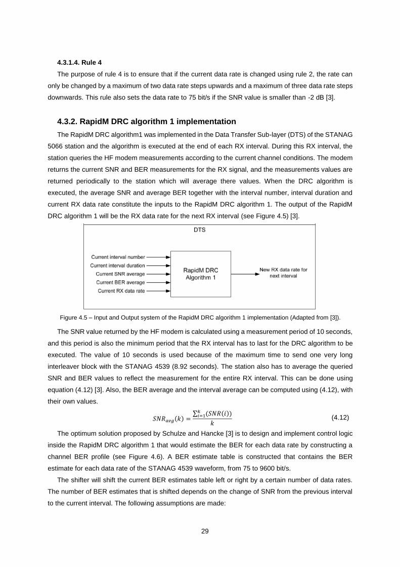
This chapter presents the simulation and assessment of the DRC algorithms described in the

previous chapter. Based on the assessment results, several improvements on those algorithms are then

proposed and evaluated.

5.1. DRC Algorithms Simulation System

In order to assess the performance of the DRC algorithms described in Chapter 4, a simulation

environment was created in Matlab code, whose flowchart is presented in Figure 5.1.

Figure 5.1 – Simulation system flowchart.

The simulation system starts with an initialization process that loads the SNR channel requirements

for a BER of 10−5 and for the considered channel type, which can be AWGN (cf. Table 3.2), ITU Good

(cf. Table 3.3) or ITU Poor (cf. Table 3.4). This process continues with the reading of the current

channel SNR, which leads to the computation of the initial data rate by comparing the current SNR with

the SNR channel requirements. After this initialization process, the data transmission between stations

starts. Periodically, the system reads the current channel SNR and computes the corresponding channel

BER and FER using equations (5.1), (5.2) and (4.5); based on these values and on the current data

rate, a new data rate value is computed by the DRC algorithm that will be applied to the following

transmission interval.

It is worth to note that (5.1) is just an approximation of the BER vs SNR, valid for the range of BER

values showing a linear variation with the SNR, in logarithmic units; as shown in Figure 5.2, for BER

34

values below 10-5 the BER decreases by one decade per +1 dB variation in SNR, which can be

expressed by (5.1).

BER = 10−5 × 10−∆SNR (5.1)

∆SNR = SNR𝑐𝑢𝑟𝑟𝑒𝑛𝑡 − SNR𝑟𝑒𝑞𝑢𝑖𝑟𝑒𝑚𝑒𝑛𝑡𝑠 (5.2)

Figure 5.2 – BER as a function of SNR for m-QAM modulation, with a straight line (in green) representing a BER variation of 1 decade per dB (Adapted from [32]).

After the BER and FER computation, the selected DRC algorithm will be applied whenever there is

still data to be transmitted; the current data rate will be then updated for the following data transmission

interval. The concept of data transmission interval (or time interval) is defined by the period between

two SNR measurements. Figure 5.3 shows the time diagram of the channel measurements - at the

beginning of each time interval, the computed BER and FER refers to the previous time interval, and

the updated data rate refers to the following interval.

Figure 5.3 – Channel measurements time diagram.

35

This process shown in Figure 5.3 is applied only in the TX station, because the transmitted frame

has a header with the current data rate, and after the RX station read the header it will update this data

rate. At the end of the transmission, the following link assessment metrics are computed:

Average Data Rate (in bits/s) – defined by (5.3), where 𝐷𝑅𝑖 is the data rate value for the interval

number 𝑖, 𝑇𝑖 is the interval duration and 𝑁 is the total number of intervals

𝐷𝑅̅̅ ̅̅ =∑ 𝐷𝑅𝑖×𝑇𝑖

𝑁𝑖=1

∑ 𝑇𝑖𝑁𝑖=1

[bit/s] . (5.3)

Average BER – defined by (5.5), where 𝐵𝐸𝑅𝑖 is the value of the computed BER for interval

number 𝑖. Whenever the BER value is higher than 10−3, it is considered that the link is in cut-off

state; an auxiliary variable, 𝜏𝑖, computed by (5.4), accounts for the time intervals that are not in

cut-off state. This metric is only counted when the link is available

𝜏𝑖(𝐵𝐸𝑅𝑖) = { 𝑇𝑖 𝑖𝑓 𝐵𝐸𝑅𝑖 ≤ 10−3

0 𝑖𝑓 𝐵𝐸𝑅𝑖 > 10−3 , (5.4)

𝐵𝐸𝑅̅̅ ̅̅ ̅̅ =∑ 𝐵𝐸𝑅𝑖 × 𝜏𝑖(𝐵𝐸𝑅𝑖)

𝑁𝑖=1

∑ 𝜏𝑖(𝐵𝐸𝑅𝑖)𝑁𝑖=1

. (5.5)

Average FER (in %) – defined by (5.6), where 𝐹𝐸𝑅𝑖 is the value of the computed FER for interval

number 𝑖. As in average BER, this metric is only counted when the link is available

𝐹𝐸𝑅̅̅ ̅̅ ̅̅ =∑ 𝐹𝐸𝑅𝑖 × 𝜏𝑖(𝐵𝐸𝑅𝑖)

𝑁𝑖=1

∑ 𝜏𝑖(𝐵𝐸𝑅𝑖)𝑁𝑖=1

× 100 [%] . (5.6)

Link Availability (in %) – defined by (5.7), is the percentage of time for which the BER value is

lower than 10−3

𝐿𝐴 =∑ 𝜏𝑖(𝐵𝐸𝑅𝑖)𝑁

𝑖=1


× 100 [%] . (5.7)

Average throughput (in bit/s) – defined by (5.8), represents the number of correct bits/s at the

receiver

𝑇ℎ̅̅̅̅ = ∑ 𝐷𝑅𝑖 × 𝜏𝑖(𝐵𝐸𝑅𝑖) × (1 − 𝐵𝐸𝑅𝑖) 𝑁

𝑖=1


[bit/s] . (5.8)

Average goodput (in frames/s) – defined by (5.9), where 𝐿 is the frame length in bits, represents

the number of correct frames/s at the receiver

𝐺𝑝̅̅̅̅ = ∑

𝐷𝑅𝑖

𝐿 × (1 − 𝐹𝐸𝑅𝑖) × 𝜏𝑖(𝐵𝐸𝑅𝑖) 𝑁

𝑖=1


[frames/s] . (5.9)

To assess the algorithms, four types of channel SNR variations have been considered: downward

sinusoidal, defined by (5.10) and represented in Figure 5.4; upward sinusoidal, defined by (5.11) and

represented in Figure 5.5; sinusoidal, defined by (5.12) and represented in Figure 5.6; and step-wise,

represented in Figure 5.7 and whose behaviour is the closest to a real channel.

SNR(t) = 15 − 25 ∗ cos ((

2π

200) × (t + 100)) [dB] (5.10)

SNR(t) = 15 + 25 ∗ cos ((

2π

200) × (t + 100)) [dB] (5.11)

36

SNR(t) = 15 − 25 ∗ cos ((

2π

66) × (t + 100)) [dB] (5.12)

Figure 5.4 – Downward sinusoidal SNR variation.

Figure 5.5 – Upward sinusoidal SNR variation.

Figure 5.6 – Sinusoidal SNR variation.

Figure 5.7 – Step-wise SNR variation.

37

For the algorithms assessment, the following parameters values were used:

interval duration (𝑇𝑖) = 120 seconds;

total number of measurement intervals (𝑁) = 100;

frame size (𝐿) = 250 bytes.

For these parameters values, equations (5.3) to (5.9) can be rewritten as:

𝐷𝑅̅̅ ̅̅ =∑ 𝐷𝑅𝑖

100𝑖=1

100 [bit/s] (5.13)

𝜏𝑖(𝐵𝐸𝑅𝑖) = {1 𝑖𝑓 𝐵𝐸𝑅𝑖 ≤ 10−3

0 𝑖𝑓 𝐵𝐸𝑅𝑖 > 10−3 (5.14)

𝐵𝐸𝑅̅̅ ̅̅ ̅̅ =∑ 𝐵𝐸𝑅𝑖 × 𝜏𝑖(𝐵𝐸𝑅𝑖)

100𝑖=1

∑ 𝜏𝑖(𝐵𝐸𝑅𝑖)100𝑖=1

(5.15)

𝐹𝐸𝑅̅̅ ̅̅ ̅̅ =∑ 𝐹𝐸𝑅𝑖

100𝑖=1 × 𝜏𝑖(𝐵𝐸𝑅𝑖)

∑ 𝜏𝑖(𝐵𝐸𝑅𝑖)100𝑖=1

[%] (5.16)

𝐿𝐴 = ∑ 𝜏𝑖(𝐵𝐸𝑅𝑖)

100

𝑖=1

[%] (5.17)

𝑇ℎ̅̅̅̅ = ∑ 𝐷𝑅𝑖 × (1 − 𝐵𝐸𝑅𝑖) × 𝜏𝑖(𝐵𝐸𝑅𝑖) 100

𝑖=1

100 [bit/s] (5.18)

𝐺𝑝̅̅̅̅ = ∑

𝐷𝑅𝑖

250 × 8 × (1 − 𝐹𝐸𝑅𝑖) × 𝜏𝑖(𝐵𝐸𝑅𝑖) 100

𝑖=1

100 [frames/s] . (5.19)

5.2. Previous DRC algorithms: Simulation and Assessment

After designing the simulation environment, the DRC algorithms reviewed on Chapter 4, namely

Trinder and RapidM algorithms, were reproduced in Matlab code. This section presents the

assessments of those algorithms, according to the simulation system described in the section 5.1, to

determine the gaps where they can be improved.

5.2.1. Trinder algorithm Simulation and Assessment

In Trinder algorithm, the appropriate data rate is based on FER thresholds; therefore, at the end of

each measurement interval the BER and FER values are computed based on the current SNR measure,

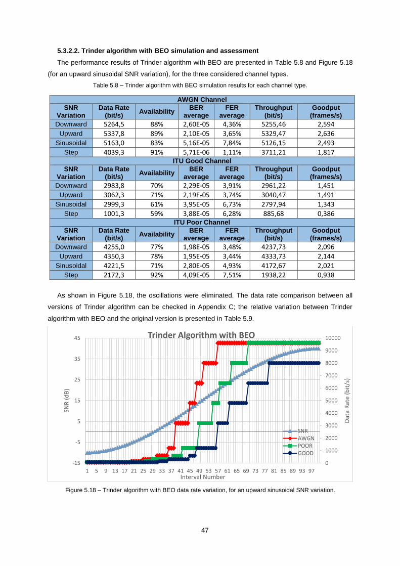
as depicted in Figure 5.3. The Trinder algorithm assessment results are represented in Table 5.1, for

the three considered channel types; Figure 5.8 shows the data rate variation for the considered

channels, and for an upward sinusoidal SNR variation.

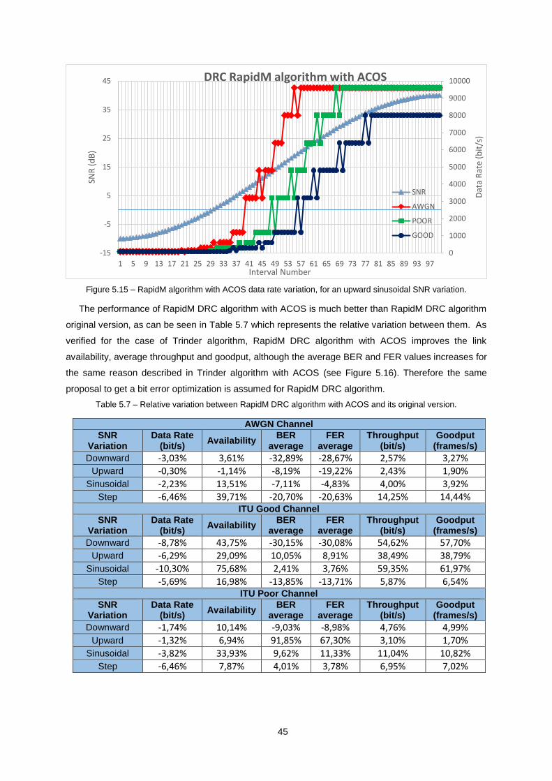
The main vulnerability detected by combining the analysis of the data rate adaption (in Figure 5.8),

the link availability results (in Table 5.1) and the BER versus data rate variation (in Figure 5.9), is the

data rate oscillations that lead to many cut-off states, reducing the link availability. If the link availability

increases, by reducing the unnecessary oscillations, it is expected that the average BER and FER will

also increase. The proposal to improve the link quality is to implement a new version of the Trinder

38

algorithm that, before updating the data rate evaluates if the new data rate will lead to the cut-off state;

if yes, the previous data rate will be kept.

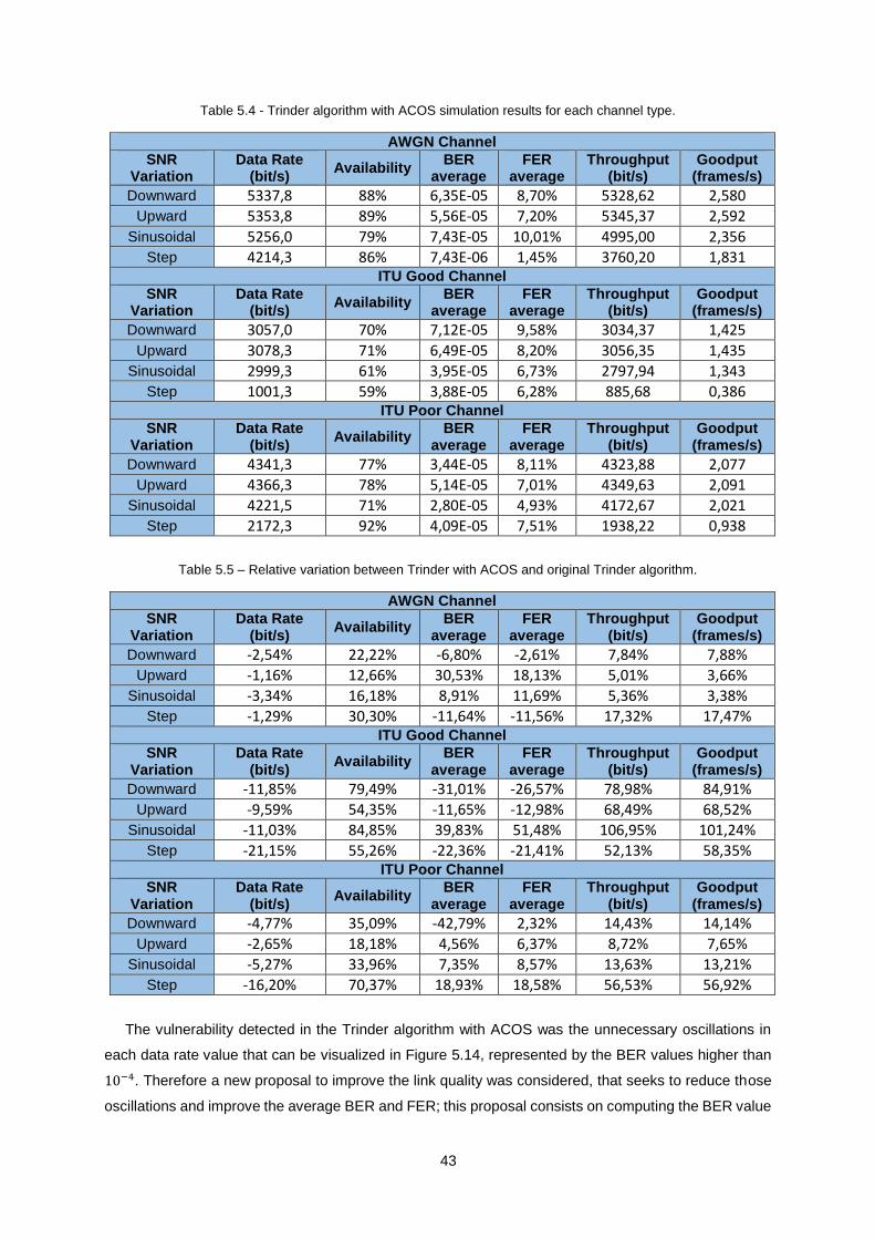
Table 5.1 – Trinder algorithm simulation results for each channel type.

AWGN Channel

SNR Variation

Data Rate (bit/s)

Availability BER

average FER

average Throughput

(bit/s) Goodput

(frames/s)

Downward 5477,0 72% 6,81E-05 8,93% 4941,38 2,391 Upward 5416,8 79% 4,26E-05 6,10% 5090,44 2,501

Sinusoidal 5437,5 68% 6,82E-05 8,96% 4741,07 2,279 Step 4269,3 66% 8,41E-06 1,64% 3205,20 1,558

ITU Good Channel

SNR Variation

Data Rate (bit/s)

Availability BER

average FER

average Throughput

(bit/s) Goodput

(frames/s)



ITU Poor Channel

SNR Variation

Data Rate (bit/s)

Availability BER

average FER

average Throughput

(bit/s) Goodput

(frames/s)

Downward 4558,5 57% 6,01E-05 7,93% 3778,65 1,819

Upward 4485,3 66% 4,91E-05 6,59% 4000,67 1,942 Sinusoidal 4456,5 53% 2,61E-05 4,54% 3672,19 1,785

Step 2592,3 54% 3,44E-05 6,33% 1238,23 0,598

Figure 5.8 – Trinder algorithm data rate variation, for an upward sinusoidal SNR variation.

0

1000

2000

3000

4000

5000

6000

7000

8000

9000

10000

-15

-5

5

15

25

35

45

1 5 9 13 17 21 25 29 33 37 41 45 49 53 57 61 65 69 73 77 81 85 89 93 97

Dat

a R

ate

(bit

/s)

SNR

(d

B)

Interval Number

Trinder Algorithm

SNR

AWGN

POOR

GOOD

39

Figure 5.9 – Trinder algorithm: BER vs Data Rate variation, for an upward sinusoidal SNR variation using an ITU Poor channel.

5.2.2. RapidM DRC algorithm Simulation and Assessment

The RapidM DRC algorithm bases the data rate decision in four rules: the first two rules compute the

next data rate based on SNR variations; the third rule preforms data rate decisions based on the

computed BER value, as in Trinder algorithm; and the fourth is a security rule that allows the data rate

to increase, at most, two steps at once, and to decrease three steps at once. The link assessment

results are represented in Table 5.2 for the three considered channel types; Figure 5.10 shows the data

rate variation for the considered channels, and for an upward sinusoidal SNR variation.

Table 5.2 – RapidM DRC algorithm simulation results for each type of channel.

AWGN Channel

SNR Variation

Data Rate (bit/s)

Availability BER

average FER

average Throughput

(bit/s) Goodput

(frames/s)



ITU Good Channel

SNR Variation

Data Rate (bit/s)

Availability BER

average FER

average Throughput

(bit/s) Goodput

(frames/s)


Sinusoidal 3242,5 37% 2,20E-05 3,91% 1748,95 0,827

Step 948,8 53% 3,35E-05 5,47% 818,20 0,365 ITU Poor Channel

SNR Variation

Data Rate (bit/s)

Availability BER

average FER

average Throughput

(bit/s) Goodput

(frames/s)



0

0,0002

0,0004

0,0006

0,0008

0,001

0

1000

2000

3000

4000

5000

6000

7000

8000

9000

10000

1 5 9 13 17 21 25 29 33 37 41 45 49 53 57 61 65 69 73 77 81 85 89 93 97

BER

Dat

a R

ate

(bit

/s)

Interval Number

Trinder algorithm - POOR - Upward

Data RateBER

40

Figure 5.10 – Original RapidM algorithm data rate variation, for an upward sinusoidal SNR variation.

The main vulnerability detected, according to the results presented in Table 5.2, Figure 5.10 and

Figure 5.11, is the unnecessary oscillations that reduce the link availability, as also identified in Trinder

algorithm. The same proposal to improve the link quality for the Trinder algorithm will be also considered

for the RapidM algorithm; if the new data rate leads to the cut-off state, the previous data rate will be

kept.

Figure 5.11 – RapidM DRC algorithm: BER vs Data Rate variation, for an upward sinusoidal SNR variation using an ITU Poor channel.

Table 5.2 allows to confirm that, comparatively to the Trinder algorithm, the RapidM DRC algorithm

has a better performance, by increasing the link availability, average throughput and goodput, and by

decreasing the average BER and FER values. The relative variation of these assessment metrics are

represented in Table 5.3, and computed using (5.20), where x is the relative variation in percentage, obj

is the RapidM algorithm metric value and ref is the reference value (obtained using the Trinder algorithm)

x =obj − ref

ref × 100 [%]. (5.20)

0

1000

2000

3000

4000

5000

6000

7000

8000

9000

10000

-15

-5

5

15

25

35

45

1 5 9 13 17 21 25 29 33 37 41 45 49 53 57 61 65 69 73 77 81 85 89 93 97

Dat

a R

ate

(bit

/s)

SNR

(d

B)

Interval Number

DRC RapidM algorithmSNR

AWGN

POOR

GOOD

0

0,0002

0,0004

0,0006

0,0008

0,001

0

1000

2000

3000

4000

5000

6000

7000

8000

9000

10000

1 5 9 13 17 21 25 29 33 37 41 45 49 53 57 61 65 69 73 77 81 85 89 93 97

BER

Dat

a R

ate

(bit

/s)

Interval Number

RapidM algorithm - POOR - Upward

Data RateBER

41

Table 5.3 – Relative variation between RapidM DRC and Trinder algorithm.

AWGN Channel

SNR Variation

Data Rate (bit/s)

Availability BER

average FER

average Throughput

(bit/s)

Goodput

(𝟏𝟎−𝟑frames/s)

Downward -1,77% 15,28% -39,13% -27,43% 2,73% 3,04%

Upward -1,87% 11,39% -27,98% -26,12% 1,44% 1,63% Sinusoidal -3,12% 8,82% -13,22% -15,46% 4,21% 2,39%

Step -2,45% 3,03% -7,40% -7,27% 0,91% 1,06% ITU Good Channel

SNR Variation

Data Rate (bit/s)

Availability BER

average FER

average Throughput

(bit/s)

Goodput


Downward -4,55% 23,08% -58,92% -47,79% 14,31% 18,90% Upward -3,83% 19,57% -36,08% -34,86% 21,28% 21,33%

Sinusoidal -3,82% 12,12% -22,16% -12,10% 29,36% 23,96% Step -25,28% 39,47% -32,90% -31,57% 40,54% 49,72%

ITU Poor Channel

SNR Variation

Data Rate (bit/s)

Availability BER

average FER

average Throughput

(bit/s)

Goodput


Downward -2,78% 21,05% -23,99% -10,29% 9,60% 8,23%

Upward -2,03% 9,09% -77,65% -70,28% 4,70% 6,37%

Sinusoidal -3,27% 5,66% -18,35% -18,56% 1,22% 1,44% Step -18,37% 64,82% -42,44% -41,79% 40,84% 41,71%

5.3. Improvements on the Trinder and RapidM Algorithms

Based on detected vulnerabilities of the Trinder and RapidM algorithms, two new versions of each

algorithm were developed and tested in the Matlab simulation environment described in section 5.1; the

first improved version performs a BER prediction to avoid the cut-off link, and was named Avoiding

Cut-Off State (ACOS); the second improved version performs an average BER optimization, and was

named Bit Error Optimization (BEO).

5.3.1. Avoiding Cut-Off State Algorithm

5.3.1.1. Algorithm design and implementation

The ACOS algorithm is based on the BER predicted value using equation (5.1), just after the DRC

algorithm be applied and a new transmission data rate obtained. Figure 5.12 shows the ACOS algorithm

flowchart, which should be introduced in the flowchart represented in Figure 5.1. It starts with the new

BER computation based on the new data rate selected by the DRC algorithm. After performing the BER

prediction, the algorithm verifies if the resulting BER value is greater than 10−3; if it is false, the data rate

is updated to the new value; if this condition is true, a new verification is performed. The algorithm checks

if the new data rate is lower than previous one; if it is false, the previous data rate is maintained; if it is

true, the new data rate is decreased.

42

Figure 5.12 – Avoiding Cut-Off State algorithm flowchart.

The ACOS is easy to implement because it is just a BER computation and two condition to be added

to the existing solutions.

5.3.1.2. Trinder algorithm with ACOS: simulation and assessment

The link data rate variation for the Trinder algorithm with ACOS is represented in Figure 5.13 (for an

upward sinusoidal SNR variation); Table 5.4 presents the assessment metrics values, and Table 5.5

presents the relative variation between both algorithms. The link availability, average throughput and

goodput have a great improvement with ACOS, the number of data rate oscillations decrease, although

the average BER and FER increase, because the link availability also increase. A graphical comparison

between Trinder algorithm with ACOS and the original version is presented in Appendix C.

Figure 5.13 – Trinder algorithm with ACOS data rate variation, for an upward sinusoidal SNR variation.

0

1000

2000

3000

4000

5000

6000

7000

8000

9000

10000

-15

-5

5

15

25

35

45

1 5 9 13 17 21 25 29 33 37 41 45 49 53 57 61 65 69 73 77 81 85 89 93 97

Dat

a R

ate

(bit

/s)

SNR

(d

B)

Interval Number

Trinder Algorithm with ACOS

SNRAWGNPOORGOOD

43

Table 5.4 - Trinder algorithm with ACOS simulation results for each channel type.

AWGN Channel

SNR Variation

Data Rate (bit/s)

Availability BER

average FER

average Throughput

(bit/s) Goodput

(frames/s)



ITU Good Channel

SNR Variation

Data Rate (bit/s)

Availability BER

average FER

average Throughput

(bit/s) Goodput

(frames/s)

Downward 3057,0 70% 7,12E-05 9,58% 3034,37 1,425



SNR Variation

Data Rate (bit/s)

Availability BER

average FER

average Throughput

(bit/s) Goodput

(frames/s)

Downward 4341,3 77% 3,44E-05 8,11% 4323,88 2,077

Upward 4366,3 78% 5,14E-05 7,01% 4349,63 2,091


Table 5.5 – Relative variation between Trinder with ACOS and original Trinder algorithm.

AWGN Channel

SNR Variation

Data Rate (bit/s)

Availability BER

average FER

average Throughput

(bit/s) Goodput

(frames/s)

Downward -2,54% 22,22% -6,80% -2,61% 7,84% 7,88% Upward -1,16% 12,66% 30,53% 18,13% 5,01% 3,66%

Sinusoidal -3,34% 16,18% 8,91% 11,69% 5,36% 3,38%


SNR Variation

Data Rate (bit/s)

Availability BER

average FER

average Throughput

(bit/s) Goodput

(frames/s)

Downward -11,85% 79,49% -31,01% -26,57% 78,98% 84,91% Upward -9,59% 54,35% -11,65% -12,98% 68,49% 68,52%

Sinusoidal -11,03% 84,85% 39,83% 51,48% 106,95% 101,24% Step -21,15% 55,26% -22,36% -21,41% 52,13% 58,35%

ITU Poor Channel

SNR Variation

Data Rate (bit/s)

Availability BER

average FER

average Throughput

(bit/s) Goodput

(frames/s)

Downward -4,77% 35,09% -42,79% 2,32% 14,43% 14,14% Upward -2,65% 18,18% 4,56% 6,37% 8,72% 7,65%

Sinusoidal -5,27% 33,96% 7,35% 8,57% 13,63% 13,21% Step -16,20% 70,37% 18,93% 18,58% 56,53% 56,92%

The vulnerability detected in the Trinder algorithm with ACOS was the unnecessary oscillations in

each data rate value that can be visualized in Figure 5.14, represented by the BER values higher than

10−4. Therefore a new proposal to improve the link quality was considered, that seeks to reduce those

oscillations and improve the average BER and FER; this proposal consists on computing the BER value

44

with the new selected data rate, and verify if this value is greater than the threshold BER, used in the

Trinder algorithm to decrease the data rate.

Figure 5.14 – Trinder algorithm with ACOS: BER vs Data Rate variation, for an upward sinusoidal SNR variation using an ITU Poor channel.

5.3.1.3. RapidM DRC algorithm with Avoiding Cut-Off State simulation and results

Table 5.6 presents the assessment metrics values for the RapidM algorithm with ACOS, and the

link data rate variation is represented in Figure 5.15 (for an upward sinusoidal SNR variation).

Table 5.6 – RapidM DRC algorithm with ACOS simulation results for each channel type.

AWGN Channel

SNR Variation

Data Rate (bit/s)

Availability BER

average FER

average Throughput

(bit/s) Goodput

(frames/s)

Downward 5217,3 86% 2,78E-05 4,62% 5206,68 2,545


Step 3895,5 95% 6,18E-06 1,21% 3695,45 1,802 ITU Good Channel

SNR Variation

Data Rate (bit/s)

Availability BER

average FER

average Throughput

(bit/s) Goodput

(frames/s)

Downward 3019,8 69% 2,96E-05 4,76% 2996,44 1,445



SNR Variation

Data Rate (bit/s)

Availability BER

average FER

average Throughput

(bit/s) Goodput

(frames/s)



0

0,0002

0,0004

0,0006

0,0008

0,001

0

1000

2000

3000

4000

5000

6000

7000

8000

9000

10000

1 5 9 13 17 21 25 29 33 37 41 45 49 53 57 61 65 69 73 77 81 85 89 93 97

BER

Dat

a R

ate

(bit

/s)

Interval Number

Trinder algorithm with ACOS - POOR - Upward

Data RateBER

45

Figure 5.15 – RapidM algorithm with ACOS data rate variation, for an upward sinusoidal SNR variation.

The performance of RapidM DRC algorithm with ACOS is much better than RapidM DRC algorithm

original version, as can be seen in Table 5.7 which represents the relative variation between them. As

verified for the case of Trinder algorithm, RapidM DRC algorithm with ACOS improves the link

availability, average throughput and goodput, although the average BER and FER values increases for

the same reason described in Trinder algorithm with ACOS (see Figure 5.16). Therefore the same

proposal to get a bit error optimization is assumed for RapidM DRC algorithm.

Table 5.7 – Relative variation between RapidM DRC algorithm with ACOS and its original version.

AWGN Channel

SNR Variation

Data Rate (bit/s)

Availability BER

average FER

average Throughput

(bit/s) Goodput

(frames/s)

Downward -3,03% 3,61% -32,89% -28,67% 2,57% 3,27%

Upward -0,30% -1,14% -8,19% -19,22% 2,43% 1,90% Sinusoidal -2,23% 13,51% -7,11% -4,83% 4,00% 3,92%


SNR Variation

Data Rate (bit/s)

Availability BER

average FER

average Throughput

(bit/s) Goodput

(frames/s)

Downward -8,78% 43,75% -30,15% -30,08% 54,62% 57,70% Upward -6,29% 29,09% 10,05% 8,91% 38,49% 38,79%

Sinusoidal -10,30% 75,68% 2,41% 3,76% 59,35% 61,97%

Step -5,69% 16,98% -13,85% -13,71% 5,87% 6,54% ITU Poor Channel

SNR Variation

Data Rate (bit/s)

Availability BER

average FER

average Throughput

(bit/s) Goodput

(frames/s)

Downward -1,74% 10,14% -9,03% -8,98% 4,76% 4,99%

Upward -1,32% 6,94% 91,85% 67,30% 3,10% 1,70%

Sinusoidal -3,82% 33,93% 9,62% 11,33% 11,04% 10,82%

Step -6,46% 7,87% 4,01% 3,78% 6,95% 7,02%

0

1000

2000

3000

4000

5000

6000

7000

8000

9000

10000

-15

-5

5

15

25

35

45

1 5 9 13 17 21 25 29 33 37 41 45 49 53 57 61 65 69 73 77 81 85 89 93 97

Dat

a R

ate

(bit

/s)

SNR

(d

B)

Interval Number

DRC RapidM algorithm with ACOS

SNR

AWGN

POOR

GOOD

46

Figure 5.16 – RapidM DRC algorithm with ACOS: BER vs Data Rate variation, for an upward sinusoidal SNR variation using an ITU Poor channel.

5.3.2. Bit Error Optimization Algorithm

5.3.2.1. Algorithm design and implementation

The main difference between ACOS and BEO algorithms is the condition block; in ACOS, the

condition avoids the link cut-off. In BEO algorithm, if the predicted BER value is greater than BER

threshold defined in the original algorithms, a new condition is verified, otherwise the new data rate is

updated. This condition verifies if the new data rate is lower than previous data rate, then the new data

rate should decrease. If the condition is false the previous data rate is kept. Figure 5.17 shows the BEO

algorithm flowchart, which is introduced in the simulation system flowchart represented in Figure 5.1.

The BEO block was implemented in the simulation environment, mentioned in section 5.1, with the

Trinder and RapidM DRC algorithms. As for the ACOS algorithm, the BEO is quite simple to implement.

Figure 5.17 – Bit Error Optimization algorithm flowchart.

0

0,0002

0,0004

0,0006

0,0008

0,001

0

1000

2000

3000

4000

5000

6000

7000

8000

9000

10000

1 5 9 13 17 21 25 29 33 37 41 45 49 53 57 61 65 69 73 77 81 85 89 93 97

BER

Dat

a R

ate

(bit

/s)

Interval Number

RapidM algorithm with ACOS - POOR - Upward

Data RateBER

47

5.3.2.2. Trinder algorithm with BEO simulation and assessment

The performance results of Trinder algorithm with BEO are presented in Table 5.8 and Figure 5.18

(for an upward sinusoidal SNR variation), for the three considered channel types.

Table 5.8 – Trinder algorithm with BEO simulation results for each channel type.

AWGN Channel

SNR Variation

Data Rate (bit/s)

Availability BER

average FER

average Throughput

(bit/s) Goodput

(frames/s)



ITU Good Channel

SNR Variation

Data Rate (bit/s)

Availability BER

average FER

average Throughput

(bit/s) Goodput

(frames/s)



ITU Poor Channel

SNR Variation

Data Rate (bit/s)

Availability BER

average FER

average Throughput

(bit/s) Goodput

(frames/s)



As shown in Figure 5.18, the oscillations were eliminated. The data rate comparison between all

versions of Trinder algorithm can be checked in Appendix C; the relative variation between Trinder

algorithm with BEO and the original version is presented in Table 5.9.

Figure 5.18 – Trinder algorithm with BEO data rate variation, for an upward sinusoidal SNR variation.

0

1000

2000

3000

4000

5000

6000

7000

8000

9000

10000

-15

-5

5

15

25

35

45

1 5 9 13 17 21 25 29 33 37 41 45 49 53 57 61 65 69 73 77 81 85 89 93 97

Dat

a R

ate

(bit

/s)

SNR

(d

B)

Interval Number

Trinder Algorithm with BEO

SNRAWGNPOORGOOD

48

The elimination of the data rate oscillations resulted in the best performance of average goodput,

BER and FER in the set of solutions presented for Trinder algorithm; this can be checked by the relative

variations presented in Table 5.5 and Table 5.9. The Trinder with ACOS and the Trinder with BEO

algorithms have similar link availability values, but the first one has better average throughput

performance. Figure 5.19 shows how the BER is maintained below the BER threshold, resulting in an

elimination of the data rate oscillations.

Table 5.9 – Relative variation between Trinder algorithm with BEO and the original version.

AWGN Channel

SNR Variation

Data Rate (bit/s)

Availability BER

average FER

average Throughput

(bit/s) Goodput

(frames/s)

Downward -3,88% 22,22% -61,79% -51,14% 6,36% 8,46% Upward -1,46% 12,66% -50,63% -40,14% 4,70% 5,41%

Sinusoidal -5,05% 22,06% -24,28% -12,54% 8,12% 9,37%


SNR Variation

Data Rate (bit/s)

Availability BER

average FER

average Throughput

(bit/s) Goodput

(frames/s)

Downward -13,96% 79,49% -77,79% -70,00% 74,66% 88,24% Upward -10,06% 54,35% -70,17% -60,29% 67,62% 75,08%

Sinusoidal -11,03% 84,85% 39,83% 51,48% 106,95% 101,24% Step -21,15% 55,26% -22,36% -21,41% 52,13% 58,35%

ITU Poor Channel

SNR Variation

Data Rate (bit/s)

Availability BER

average FER

average Throughput

(bit/s) Goodput

(frames/s)

Downward -6,66% 35,09% -67,09% -56,11% 12,15% 15,21%

Upward -3,01% 18,18% -60,23% -47,85% 8,33% 10,40% Sinusoidal -5,27% 33,96% 7,35% 8,57% 13,63% 13,21%

Step -16,20% 70,37% 18,93% 18,58% 56,53% 56,92%

Figure 5.19 – Trinder algorithm with BEO: BER vs Data Rate variation, for an upward sinusoidal SNR variation using an ITU Poor channel.

0

0,0002

0,0004

0,0006

0,0008

0,001

0

1000

2000

3000

4000

5000

6000

7000

8000

9000

10000

1 5 9 13 17 21 25 29 33 37 41 45 49 53 57 61 65 69 73 77 81 85 89 93 97

BER

Dat

a R

ate

(bit

/s)

Interval Number

Trinder algorithm with BEO - POOR - Upward

Data Rate

BER

49

5.3.2.3. RapidM algorithm with BEO simulation and assessment

The performance results of the RapidM algorithm with BEO are represented in Table 5.10 and Figure

5.20 (for an upward sinusoidal channel), for the three types of channels. According to the results, the

oscillations were eliminated (like in Tinder algorithm with BEO), and the average BER and FER had

great performance improvements.

The relative variation between the RapidM algorithm with BEO and the original version is represented

in Table 5.11, and Figure 5.21 shows how the BER is maintained below the BER threshold of RapidM

DRC algorithm.

Table 5.10 – RapidM DRC algorithm with BEO simulation results for each channel type.

AWGN Channel

SNR Variation

Data Rate (bit/s)

Availability BER

average FER

average Throughput

(bit/s) Goodput

(frames/s)

Downward 5217,3 86% 6,92E-06 3,83% 5206,73 2,588


Step 3895,5 95% 6,18E-06 1,21% 3695,45 1,802 ITU Good Channel

SNR Variation

Data Rate (bit/s)

Availability BER

average FER

average Throughput

(bit/s) Goodput

(frames/s)


Sinusoidal 2860,5 66% 1,49E-05 2,74% 2834,97 1,390


SNR Variation

Data Rate (bit/s)

Availability BER

average FER

average Throughput

(bit/s) Goodput

(frames/s)

Downward 4259,8 76% 8,58E-06 1,64% 4241,73 2,097

Upward 4336,0 77% 6,05E-06 1,16% 4318,73 2,142


Figure 5.20 – RapidM algorithm with BEO data rate variation, for an upward sinusoidal SNR variation.

0

1000

2000

3000

4000

5000

6000

7000

8000

9000

10000

-15

-5

5

15

25

35

45

1 5 9 13 17 21 25 29 33 37 41 45 49 53 57 61 65 69 73 77 81 85 89 93 97

Dat

a R

ate

(bit

/s)

SNR

(d

B)

Interval Number

DRC RapidM algorithm with BEO

SNRAWGNPOORGOOD

50

Table 5.11 – Relative variation between RapidM DRC algorithm with BEO and the original version.

AWGN Channel

SNR Variation

Data Rate (bit/s)

Availability BER

average FER

average Throughput

(bit/s) Goodput

(frames/s)

Downward -3,03% 3,61% -83,32% -40,98% 2,57% 5,03% Upward -0,66% -1,14% -78,68% -72,23% 2,07% 3,18%

Sinusoidal -3,62% 13,51% -83,93% -76,22% 2,52% 7,47% Step -6,46% 39,71% -20,70% -20,63% 14,25% 14,44%

ITU Good Channel

SNR Variation

Data Rate (bit/s)

Availability BER

average FER

average Throughput

(bit/s) Goodput

(frames/s)

Downward -11,17% 43,75% -83,65% -80,56% 50,53% 57,51%

Upward -7,85% 29,09% -77,69% -69,85% 36,18% 43,53% Sinusoidal -11,78% 78,38% -32,38% -29,78% 62,10% 68,06%

Step -16,23% 16,98% -74,33% -71,92% -6,35% 1,50% ITU Poor Channel

SNR Variation

Data Rate (bit/s)

Availability BER

average FER

average Throughput

(bit/s) Goodput

(frames/s)

Downward -3,89% 10,14% -81,22% -77,00% 2,46% 6,51%

Upward -1,32% 6,94% -44,87% -40,61% 3,10% 3,68%

Sinusoidal -4,56% 33,93% -25,27% -22,15% 10,18% 11,34% Step -6,46% 7,87% 4,01% 3,78% 6,95% 7,02%

Figure 5.21 – RapidM DRC algorithm with BEO: BER vs Data Rate variation, for an upward sinusoidal SNR variation using an ITU Poor channel.

0

0,0002

0,0004

0,0006

0,0008

0,001

0

1000

2000

3000

4000

5000

6000

7000

8000

9000

10000

1 5 9 13 17 21 25 29 33 37 41 45 49 53 57 61 65 69 73 77 81 85 89 93 97

BER

Dat

a R

ate

(bit

/s)

Interval Number

RapidM algorithm with BEO - POOR - Upward

Data Rate

BER

51

5.4. Conclusion

The improvements presented in section 5.3 for the Trinder and RapidM algorithms worked as

excepted and had better outcomes than the existing solutions, for the considered channel types and

SNR variations. The following classification for all the improvement proposals and the existing solutions

were recorded, based on the relative variation and the simulation results tables, for each type of link

assessment metric:

Lowest average BER – RapidM DRC algorithm with BEO

Lowest average FER – RapidM DRC algorithm with BEO

Highest link availability – RapidM DRC algorithm with BEO

Highest average throughput – Trinder algorithm with ACOS

Highest average goodput – Trinder algorithm with BEO

As the DRC algorithms main objective is to transmit the largest number of correct frames, to prevent

frame retransmission (because of ARQ protocol), the Trinder algorithm with BEO is the algorithm with

best performance. For future work it is advisable to implement an algorithm that changes the frame size

according to the link quality metrics, since the DRC algorithm assessments were performed with a

constant frame size. If the BER increased, the frame size should decrease to keep the same FER value,

as can be checked in (4.5).

52

53

6. Chapter 6 – Field Propagation Tests

This chapter presents the hardware and software components involved in the field propagation tests

as well the obtained results. An user interface application was developed in C#, using the Microsoft

Visual Studio to allow the radio operator to easily interact with the radio equipment through a serial port.

The application was initially tested on a bench circuit for error checking, to test the application

functionalities, to evaluate the limits of SNR measurements and the proper behaviour of the algorithms.

Finally, field tests were conducted with two stations, each with one E/R GRC-525 radio and

one RF-1936P dipole antenna (as showed in Figure 6.1). The two stations were located in the

Portuguese cities of Lisbon and Oporto, with a link distance of about 300 km. The E/R GRC-525 radio

and RF-1936P antenna datasheets are presented in Appendices A and B, respectively.

Figure 6.1 – Dipole antenna RF-1936P from Harris Corporation.

6.1. Equipment Assembly and Configuration Procedures

The tests of the several DRC algorithms were divided in two phases: the initial bench circuit tests

and the field propagation tests. In the first phase it was intended to test the functionality of the developed

application, the behaviour of the implemented algorithms, the channel quality for extreme SNR

conditions and the behaviour of the radio in terms of the range of the output parameters. To accomplish

the goals of the first phase a bench circuit was assembled with a variable attenuator, which allows to

test the radio measurements, such as the SNR and BER values, when the LQA Table command is

executed. This command is included in a confidential list of commands for radio operation by serial port

or over IP (this list was consulted on [33]).

The following phase was to test the algorithms on the field, when all the parameters of the previous

phase were already approved, to be sure that the only variable to affect the data rate choice is the

propagation conditions. To test the algorithms on a battlefield like scenario, a link was established

between the Logistics Support Unity, in Lisbon, and the Signals Regiment, in Oporto, 282 km apart. The

tests were performed in a period of nine days, almost at the same time of day, to have similar

propagation conditions to compare the performance of the several algorithms.

54

6.1.1. General Settings and Components

6.1.1.1. Ionospheric Study and Communications Plan

Before proceeding with the stations assembly, it was necessary to plan the communication mission

and study the behaviour of the Ionosphere for the testing days. In Portugal, military HF communications

require that frequencies are requested to the Direction of Communications and Information Systems

(DCSI) which was done using the Electrical Message document, presented in Appendix D. In this

document the frequency band limits had to be specified. With this purpose the graph of the Figure 6.2

was analysed and the frequencies selected to be between 4 MHz and 8 MHz, because the tests period

were between 9 h and 17 h. In Figure 6.2, the white line corresponds to the expected value during 28th

August 2017, and the red line corresponds to the real values measured by the ionosondes. In this case

the channel was stable and the measured values match the expected values.

Figure 6.2 – Critical frequency of F2 layer in real time for the 28th of August 2017 (Consulted on [17]).

Another important concern is to verify if the MUF values are stable too, for the time period defined to

perform the field propagation tests. Figure 6.3 a) shows three different lines of MUF during the day (28th

August 2017) for three different frequencies within the limits defined previously, therefore, with these

MUF values it was possible to verify that the HF communications were stable in the time period between

9h and 17h, as shown in Figure 6.3 a).

There are other important facts that may interfere with the stability of the HF communications, and

can influence the expected values. These facts are related with the geomagnetic storms, the HF fadeout

and the HF communication warnings. A geomagnetic storm is a major Earth magnetic fields disturbance

that occurs when there is a very efficient exchange of energy from the solar wind into the space

environment surrounding Earth [34] and this results in geomagnetic warnings. The HF fadeout results

from the solar flares and it mostly have an onset of a few minutes and a slower decline lasting an hour

[35]. The HF communication warning is related with Ionospheric storms or disturbances; these warnings

can be verified in Figure 6.3 b).

55

a) b)

Figure 6.3 – Real time Ionospheric data for the 28th August 2017: a) MUF values in percentage during the day (Consulted on [36]); b) Warnings that may influence the HF communications (Consulted on [17]).

After the Ionospheric study and frequency analysis, the Electrical Message (presented in Appendix

D) was submitted to DCSI, requesting frequencies between 4 MHz and 8 MHz. The eight frequencies

presented in Appendix H were assigned for the field tests.

With the frequencies scan group already defined, the communication mission was programmed in

3G-ALE mode at the two stations. The chosen interleaver for this HF communication was the long one,

with a 250 bytes length of data frame block, as was used in the Matlab simulations, described in Chapter

5, and the LQA exchange time between stations was 5 minutes. A Fill Gun HQ was used to transfer the

mission to the radio, as can be seen in the Figure 6.4. The mission was uploaded from the computer to

the fill gun, and then it was downloaded from the fill gun into the radio E/R GRC-525.

a) b)

Figure 6.4 – Process of downloading the mission on the radio: a) Fill Gun HQ produced by EID; b) Data transfer from the Fill Gun HQ to the E/R GRC-525.

56

6.1.1.2. Methodology of Radio Operation

After downloading the communication mission into the radio, it is necessary to verify that the ratio

between the reflected wave power and the transmission power is less than 0.1. This fact can be

expressed by the condition in equation (6.1), being 𝑃𝑟 the reflected wave power (in Watt) and 𝑃𝑇 the

transmission power (in Watt). The measured reflected wave power is performed with a wattmeter as

showed in Figure 6.5.

𝑃𝑟 ≤ 0.1 × 𝑃𝑇 (6.1)

a) b)

Figure 6.5 – Wattmeter used to verify the reflected wave power of each frequency: a) Image of the wattmeter produced by Bird Electronic Corporation; b) Practical use of the wattmeter.

If everything is fine with the reflected wave power, it is necessary to tune the antenna with the radio.

This process is done with the Antenna Tuning Unity (ATU), which is located in the HF/VHF power

amplifier. The transmission signal is amplified in the 1.5 MHz to 30 MHz frequency range and it filters

the signal harmonics. The ATU process is initialized through the radio menu, as shown in Figure 6.6 a);

if the tuning failed the screen shows the following message: “ANTENNA TUNE FAILED”. If the tuning is

performed successfully the screen shows the message “ATU LEARN O.K.”, shown in Figure 6.6 b).

a) b)

Figure 6.6 – ATU learning process: a) ATU learning the group of eight available frequencies; b) Message when the tuning is performed successfully.

57

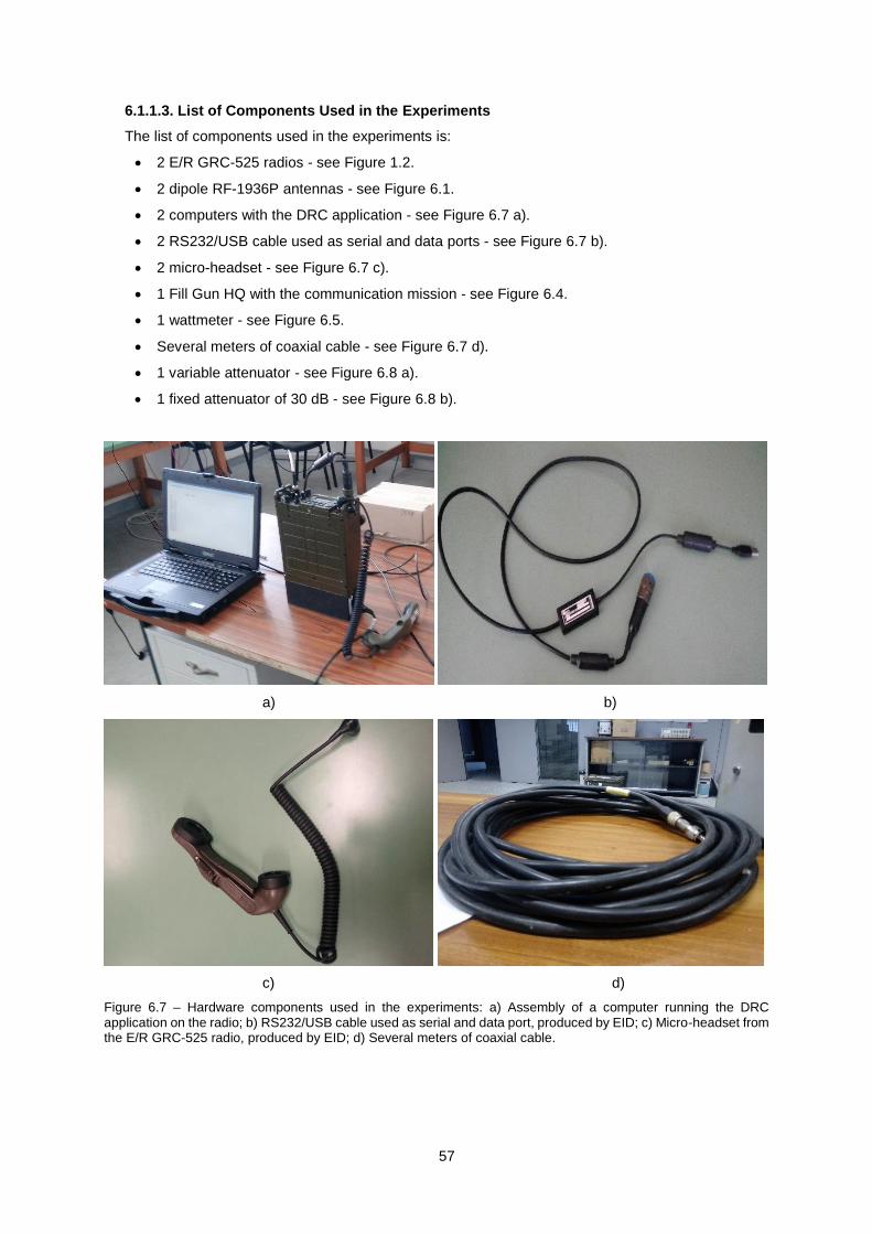
6.1.1.3. List of Components Used in the Experiments

The list of components used in the experiments is:

2 E/R GRC-525 radios - see Figure 1.2.

2 dipole RF-1936P antennas - see Figure 6.1.

2 computers with the DRC application - see Figure 6.7 a).

2 RS232/USB cable used as serial and data ports - see Figure 6.7 b).

2 micro-headset - see Figure 6.7 c).

1 Fill Gun HQ with the communication mission - see Figure 6.4.

1 wattmeter - see Figure 6.5.

Several meters of coaxial cable - see Figure 6.7 d).

1 variable attenuator - see Figure 6.8 a).

1 fixed attenuator of 30 dB - see Figure 6.8 b).

a) b)

c) d)

Figure 6.7 – Hardware components used in the experiments: a) Assembly of a computer running the DRC application on the radio; b) RS232/USB cable used as serial and data port, produced by EID; c) Micro-headset from the E/R GRC-525 radio, produced by EID; d) Several meters of coaxial cable.

58

a) b)

Figure 6.8 – Hardware components used specifically for bench experiments: a) Variable HF attenuator, produced by EID; b) Fixed attenuator of 30 dB to assembly on the transmitter output.

6.1.2. Assembly of Bench Tests Circuit

The bench circuit was assembled to test the application functionalities, such as problems in the

functionality of the algorithms, verification of the output files, test the limits of the radio as well the

parameters received. As part of the bench test circuit, a 0-90 dB variable HF attenuator (see Figure

6.8 a)) was used to control the output power of the system and simulate the environment changes.

The transmission power used in these bench experiences was 500 mW. The two radio terminals

were connected with a 15 m coaxial cable, shown in Figure 6.7 d). It was necessary to put a fixed

attenuator at the output of the transmission terminal, as shown in Figure 6.8 b), to avoid high power

peaks that can damage the equipment. The schematic of the bench circuit is represented in Figure 6.9.

The physical assembly is shown in Figure 6.10 with the two stations, each composed by one computer

running the DRC application, one E/R GRC-525 radio, one RS232/USB cable and one micro-headset,

implementing what is in the schematic.

Figure 6.9 – Schematic of the bench circuit used to test the DRC application.

59

a) b)

Figure 6.10 – Physical assembly of the bench tests circuit: a) Output system with a TX station and the fixed attenuator of 30 dB; b) Input system with the RX station and the variable HF attenuator.

6.1.3. Assembly of Field Tests Equipment

The main objective of the field propagation tests is to recreate a real battlefield environment where

the HF communications can be used; therefore, a BLOS link must be established with a large distance.

In Portugal there are two signals units with the appropriate equipment in Lisbon and Oporto, which are

separated by almost 300 km.

Both stations are composed by one E/R-GRC525 radio, one dipole antenna RF-1936P, one micro-

headset, one RS232/USB cable and one computer with the software application running, named DRC

application. The connection distance is 282 km, being the Station 1 located in the Logistics Support

Unity, Paço de Arcos, Lisbon and the Station 2 located in the Signals Regiment, Viso de Baixo, Oporto;

the stations locations are represented in Figure 6.11, provided by Google Maps.

a) b)

Figure 6.11 – Location of the HF stations: a) Station one located in Logistics Support Unity, Paço de Arcos, Lisbon; b) Station two located in the Signals Regiment, Viso de Baixo, Oporto.

60

Appendix E presents some pictures of the station assembly in the Logistics Support Unity, located

in Lisbon and all the concerns about the assembly of the dipole antenna used to perform the field

propagation tests. Figure 6.12 represents the two stations occupying an area of 225 m2 and a height of

4.6 m.

a) b)

Figure 6.12 – Image of the two dipole antennas RF-1936P used to perform the field propagation tests: a) Antenna located in the Signals Regiment, Viso de Baixo, Oporto; b) Antenna located in Logistics Support Unity, Paço de Arcos, Lisbon.

6.2. Data Rate Change Software Application

The DRC software application was developed in a Visual Studio environment using the C#

programming language, which is objected oriented and has specific methods to work with

communications using serial ports. The object oriented language is easy to handle and the Visual Studio

provides a graphical view to interact with the user. The reference used to learn the base syntax of the

C# language was the tutorial in [37].

The C# language was developed by Microsoft, so the application software will not work in other

operating systems, unless it is Windows. To run the application on older operating systems, such as

Windows 7 and Windows XP, the .NET framework version must be changed according to the Windows

requirements.

6.2.1. User Application Configuration

The DRC application has a graphical user interface. When the application runs it shows a window

with four tab pages with the following names: Output, Configurations, Algorithms and Graphic View. The

first thing to do, after the application initialization, is to fill the directory field identifying where the output

files will be created, as shown in Figure 6.13. In the Output tab page there is a field to send commands

to interact with the radio remote control and an output window of the radio remote control answers.

61

Figure 6.13 – Output tab page of the DRC application.

The next step is to set the communication parameters in the Configurations tab page. For this the

remote control port must be opened, choosing the higher port from the list of COM created by the DRC

application. After choosing the remote control port, the radio operation mode must be chosen between

Monitoring and Operational mode. The Monitoring mode can only be used to record and display the

values provided by the radio, while the Operational mode allows to change radio values and set

communication parameters. One of the algorithms tasks is to set the radio transmission data rate, so

the Operational mode must be used.

Figure 6.14 shows the previously described settings and the radio pre-set pages, which should be

chosen in the page with the 3G-ALE mission. When the Open button is pressed, the red colour of the

remote control field should change to green. After opening the remote control port, the Starting Sounding

button should be pressed and a call must be initiated to the other station, in order to get the

communication quality parameters, such as the BER and the SNR. The interleaver size should also be

selected in this tab page, as shown in Figure 6.14. For the field propagation tests the long size interleaver

must be defined.

a) b) c)

Figure 6.14 – Configuration tab page from the DRC application: a) Parameters to open the remote control port and starting the channel sounding; b) Signal when the remote control is open: green light when the remote control port is open and red light when it is closed; c) Field to set the interleaver size.

The next step is to choose the algorithm to use in the data transmission. It can be done in the

Algorithms tab page, identifying the type of channel, type of algorithm and number of version fields.

When this is applied, the initial data rate is defined based on the SNR value of the radio sounding. Then,

the following step is to open the data send port, which is the COM value before the remote control port

value (e.g. if the remote control port value is COM4, then the data send port value is COM3). When the

“data send” port value is opened the red colour should switches to green. All this configuration process

in the tab page Algorithms is shown in Figure 6.15, which represents the data sending settings.

62

a) b)

Figure 6.15 – Algorithms tab page from the DRC application: a) Type of algorithm, type of channel and number of version settings; b) Process to open the data send port.

The following step is to send a short message or a file to the other station established in the 3G-ALE

mission. The DRC application has the function to create and send a complete file, or exchange short

messages like in a chat. The process to create a file is shown in Figure 6.16 a). It requires to fill the

fields in the Creating File section, such as the directory of the created file, the name of the file and the

size in megabytes. After having the file, it can be sent in the Sending File section, filling the file directory

field and pressing the button Send, as shown in Figure 6.16 b). Finally, when the file is being sent, the

algorithm will start to perform the data rate transitions according to the SNR and BER values provided

by the LQA sounding.

a)

b)

Figure 6.16 – Handling files in the DRC application: a) Create a file with a defined name and size; b) Sending the created file.

6.2.2. Output Files and Graphical Views

The use of output files is to facilitate the understanding and organization of received data; therefore

two files were created for handling the information. One of the created files is used to handle the SNR

and BER data sent by the radio to the computer. This is a text file created with the current date as the

file name (e.g. the file name is “14052017.txt”, corresponding to the file created in May 14, 2017). With

this created file the algorithm will read the link quality parameters and set the data rate according to the

radio commands, consulted in the Rhode & Schwarz GB2 Platform Protocol [33].

63

The second created text file has the current data coupled to the word results (e.g. the file name is

“Results14052017.txt”, corresponding to the file created in May 14, 2017). This file allows to see the

values of data rate used, the time interval, the type of algorithm used, the BER, FER and SNR value for

each measure, and the channel used in each communication interval. With these files created on each

day of testing, it was possible to organize the results tables presented in the Appendix F, to classify the

performance of each algorithm.

The DRC application also has a graphical view to become more “user-friendly”; this view shows the

SNR measures and the defined data rate for each time interval and it is an initial prototype to facilitate

data understanding for a recent application user; it is shown in Figure 6.17 when the button Plot is

pressed.

Figure 6.17 – DRC application graphical view with the interval of SNR measures and data rate settings.

This process is only applied in the TX station, because the transmitted frame has a header with the

current data rate, and after the RX station read the header it will update this data rate. The RX station

only receives the LQA values from the channel sounding.

6.3. Field Propagation Tests: Environment Conditions and Results

The field propagation tests were divided in six days, one day for each algorithm, due to the protection

of the equipment, because transmitting with a power of 20 W overheats the radio and can damage the

internal hardware circuits. The radio transmits the data without interruption with channel sounding

simultaneously, therefore it is important to protect the normal operation of the radio to not overload it.

The meteorological and the ionospheric conditions should be recorded to compare algorithms

performances in similar conditions. To have the maximum data of environment conditions the values of

meteorological conditions, geomagnetic and fadeout warnings, critical frequency of the F2 layer (foF2)

and MUF were recorded for each day of tests.

During the field propagation tests the following variables were recorded by each station: receiver

station, used channel, current time (date-time format), time interval (in seconds), current BER, FER,

SNR, data rate, and the computed values of throughput and goodput. These data is presented in

Appendix F and allow to correlate the expected values computed by the simulation system, described

in Chapter 5, and the obtained values in the field propagation tests.

64

6.3.1. Meteorological and Ionospheric Conditions for Test Days

This section describes the factors that may influence the communication environment. These factors

can be related with meteorological conditions or atmospheric events which change the Ionosphere. The

meteorological data was consulted on the Impala Multimedia website [38] and the Ionospheric conditions

on the AMSAT-CT website [17]; Table 6.1 shows the important meteorological and Ionospheric factors,

and Appendix G the MUF and foF2 measures for each of the test days are presented.

Table 6.1 – Meteorological conditions and Ionospheric warnings for test days.

Day 30/08/2017 31/08/2017 01/09/2017 04/09/2017 05/09/2017 07/09/2017

Algorithm RapidM DRC RapidM DRC with ACOS

RapidM DRC with BEO

Trinder Trinder

with ACOS

Trinder

With BEO

Start Time (hh:mm:ss)

11:03:02 11:18:40 09:43:09 14:42:41 12:06:40 14:42:32

Finish Time (hh:mm:ss)

12:12:00 12:11:43 10:37:29 15:38:57 12:46:12 15:27:56

Lisbon Temperature

(ºC) 23,8 25,1 18,5 20,1 24,8 29,3

Porto Temperature

(ºC) 21,7 23,0 17 21,9 22,0 24,7

Weather Conditions

Cloudy Sky Little Rainfall

Clean Sky Clean Sky High

Clouds Clean Sky Clean Sky

Ionospheric Warnings

Geomagnetic Warning

Geomagnetic Warning

Geomagnetic Warning

Fadeout Warning

Fadeout Warning

Communications Fadeout

Geomagnetic Warnings

6.3.2. Algorithms Performance in Real Test Conditions

The overall results of the field propagation tests are shown in Table 6.2, with the worst performance

marked in red colour and the best performance in green colour. These overall results are computed with

the set of values presented in Appendix F. The Trinder algorithm is the algorithm with the worst

performance presenting the average FER, throughput and goodput with the most undesirable values,

such as expected in the simulation environment, and the RapidM DRC algorithm with BEO is the

algorithm with the best overall performance presenting the link availability, average throughput and

goodput with the most desirable values.

Table 6.2 – Overall results of the field propagation tests.

Algorithm Day

Total Time

(s)

Average BER

Average FER

Average SNR (dB)

Throughput (bit/s)

Goodput (frames/s)

Link Availability

RapidM 30/ago/17 4138 5,08E-06 0,89% 9,501 379,60 188,3E-3 83,88%

RapidM ACOS 31/ago/17 3183 6,69E-05 9,26% 9,328 892,22 369,0E-3 95,95%

RapidM BEO 01/set/17 3260 2,76E-04 24,98% 9,548 2425,23 927,1E-3 99,17%

Trinder 04/set/17 3376 3,69E-04 34,03% 3,971 245,61 78,9E-3 83,29%

Trinder ACOS 05/set/17 2372 1,82E-04 18,49% 4,980 1508,52 698,8E-3 86,38%

Trinder BEO 07/set/17 2724 2,68E-04 24,53% 3,383 718,94 228,3E-3 96,44%

65

In the simulation environment the Trinder algorithm with BEO represents the algorithm with best

average goodput, but in these field propagation results it appears in the third worst position of the

performance rank. One of the reasons why this happens is because the average SNR presents large

differences between the two trials, being the worst case in these field propagation results; therefore it is

important to do an analysis again in the simulation system, carrying the real SNR measurements as

input values into the simulation system.

To understand the behaviour of the algorithms as well as the differences between the SNR variations

during each day of tests, a graphical view of the SNR variation and the data rate adaptation is needed.

Figures 6.18 – 6.23 show the data rate adaptation to a SNR variation measured on each test day by the

E/R GRC-525 radio station.

According to the figures of the data rate adaptation, for each algorithm in different days, it is possible

to see that the Trinder algorithm presents several oscillations cycles, while the RapidM DRC algorithm

is more stable and careful in the data rate change, avoiding unnecessary oscillations. Also, it is possible

to see the different SNR measurements between the test days, and how the HF communication

warnings influence the link quality; as can be seen in Figure 6.23 and in Table 6.2, the average SNR for

the 7th September 2017 test is the lowest, because in this day were recorded the highest number of HF

communications warnings (HF Communication, HF Fadeout and Geomagnetic warnings).

Figure 6.18 – Data rate adaption for a SNR variation measured in 30th August 2017, using the original DRC RapidM algorithm.

0

1000

2000

3000

4000

5000

6000

-15

-10

-5

0

5

10

15

20

25

11

:03

:02

11

:30

:17

11

:30

:29

11

:30

:32

11

:36

:34

11

:43

:53

11

:43

:58

11

:44

:01

11

:44

:05

11

:44

:07

11

:51

:19

11

:51

:21

12

:01

:15

12

:01

:25

12

:01

:28

12

:01

:30

12

:02

:17

12

:02

:38

12

:02

:43

12

:03

:01

12

:03

:03

12

:03

:05

12

:04

:39

12

:12

:00

Dat

a R

ate(

bit

/s)

SNR

(dB

)

Time (hh:mm:ss)

30th August 2017 - DRC RapidM

SNR

Data Rate

66

Figure 6.19 – Data rate adaption for a SNR variation measured in 31st August 2017, using the DRC RapidM algorithm with ACOS.

Figure 6.20 – Data rate adaption for a SNR variation measured in 1st September 2017, using the DRC RapidM algorithm with BEO.

0

1000

2000

3000

4000

5000

6000

-15

-10

-5

0

5

10

15

20

25

11

:18

:40

11

:19

:01

11

:19

:12

11

:21

:11

11

:22

:22

11

:25

:25

11

:33

:49

11

:41

:46

11

:41

:52

11

:47

:54

11

:48

:00

11

:57

:25

11

:57

:30

11

:59

:24

11

:59

:28

11

:59

:38

11

:59

:45

12

:00

:04

12

:00

:41

12

:02

:05

12

:02

:11

12

:02

:16

12

:02

:32

12

:02

:43

12

:03

:02

12

:03

:11

12

:03

:47

12

:11

:39

Dat

a R

ate(

bit

/s)

SNR

(dB

)

Time (hh:mm:ss)

31st August 2017 - DRC RapidM with ACOS

SNR

Data Rate

0

1000

2000

3000

4000

5000

6000

-15

-10

-5

0

5

10

15

20

25

11

:18

:40

11

:18

:59

11

:19

:09

11

:19

:13

11

:21

:11

11

:21

:25

11

:22

:26

11

:26

:00

11

:33

:49

11

:33

:53

11

:41

:50

11

:47

:49

11

:47

:54

11

:47

:59

11

:57

:19

11

:57

:26

11

:57

:30

11

:57

:37

11

:59

:26

11

:59

:30

11

:59

:38

Dat

a R

ate(

bit

/s)

SNR

(dB

)

Time (hh:mm:ss)

1st September 2017 - DRC RapidM with BEO

SNR

Data Rate

67

Figure 6.21 – Data rate adaption for a SNR variation measured in 4th September 2017, using the original Trinder algorithm.

Figure 6.22 – Data rate adaption for a SNR variation measured in 5th September 2017, using the Trinder algorithm with ACOS.

0

1000

2000

3000

4000

5000

6000

-15

-10

-5

0

5

10

15

20

25

Dat

a R

ate(

bit

/s)

SNR

(dB

)

Time (hh:mm:ss)

4th September 2017 - Trinder

SNR

Data Rate

0

1000

2000

3000

4000

5000

6000

-15

-10

-5

0

5

10

15

20

25

12

:06

:40

12

:10

:46

12

:15

:04

12

:20

:33

12

:22

:06

12

:22

:27

12

:22

:44

12

:24

:23

12

:26

:33

12

:26

:56

12

:27

:10

12

:27

:34

12

:29

:37

12

:29

:46

12

:30

:03

12

:30

:19

12

:32

:11

12

:32

:27

12

:32

:43

12

:32

:56

12

:33

:09

12

:33

:40

12

:35

:12

12

:35

:34

12

:35

:48

12

:36

:09

Dat

a R

ate(

bit

/s)

SNR

(dB

)

Time (hh:mm:ss)

5th September 2017 - Trinder with ACOS

SNR

Data Rate

68

Figure 6.23 – Data rate adaption for a SNR variation measured in 7th September 2017, using the Trinder algorithm with BEO.

6.4. Relation between Simulations and Field Propagation Values

During the field propagation tests the SNR was one of the parameters recorded by the radio station

equipment. In order to check the simulation model, these recorded SNR values were given as an input

of the simulation system, and the simulation results compared with the field propagation results. This

analysis is presented in this section.

The next step was to compute the cross-correlation coefficients between the data rate results of the

field propagation tests and the simulated data rate for each channel type. The cross-correlation

coefficients are shown in Table 6.3 for each tested algorithm in different days, and the corresponding

chart in Figure 6.24.

Table 6.3 – Cross-correlation coefficients values between the field propagation tests results and the excepted results provided by the simulation system.

Type of Algorithm

Type of Channel

RapidM RapidM ACOS RapidM BEO Trinder Trinder ACOS Trinder BEO

30/08/2017 31/08/2017 01/09/2017 04/09/2017 05/09/2017 07/09/2017

AWGN 0,67766 0,83378 0,85398 0,25174 0,91184 0,84565

POOR 0,59605 0,83946 0,82486 0,16973 0,86288 0,77291

GOOD 0,44352 0,75186 0,87813 0,18590 0,83376 0,73656

0

1000

2000

3000

4000

5000

6000

-15

-10

-5

0

5

10

15

20

25

14

:42

:32

14

:42

:35

14

:49

:59

14

:50

:06

14

:50

:12

14

:51

:09

14

:51

:13

14

:52

:35

14

:52

:57

14

:53

:10

14

:53

:13

14

:53

:18

15

:07

:43

15

:07

:45

15

:07

:47

15

:16

:30

15

:17

:56

15

:18

:09

15

:18

:13

15

:18

:17

15

:25

:09

15

:25

:24

15

:26

:58

15

:27

:00

15

:27

:03

15

:27

:21

15

:27

:23

15

:27

:40

Dat

a R

ate(

bit

/s)

SNR

(dB

)

Time (hh:mm:ss)

7th September 2017 - Trinder with BEO

SNR

Data Rate

69

Figure 6.24 – Cross-correlation coefficient values between the field propagation tests and the expected results provided by the simulation system (graphic representation).

According to the cross-correlation coefficient values represented in Figure 6.24 and Table 6.3, the

field propagation results corresponds approximately to the expected results provided by the simulation

system most of the time. The cross-correlation coefficient value was superior to 0.8 in four out of six test

days, presenting one day (31st August 2017) closer to the ITU Poor channel type, another day

(1st September 2017) closer to the ITU Good channel type and the two other days (5th September 2017

and 7th September 2017) closer to the AWGN channel type.

The tested algorithms can also be different than simulation predictions, showed by the combining

analysis of Figure 6.26 and Figure 6.21, in which the cross-correlation coefficient value is around 0.25,

and it presents the worst cross-correlation, for the 4th September 2017, using original version of Trinder

algorithm. Otherwise, Figure 6.25 shows the best cross-correlation which can be compared with Figure

6.22, for the 5th September 2017 using the Trinder algorithm with ACOS, with a cross-correlation

coefficient value of 0.91.

Table 6.4 shows the relation between the field propagation results and the expected results for each

type of channel. It also shows that the original RapidM DRC tested on 30th August 2017 has similar

throughput results to the expected for an ITU Good channel type, but the cross-correlation coefficient

shows that the field propagation behaviour is closer to the behaviour expected for an AWGN channel.

Otherwise, the Trinder algorithm with ACOS tested on 5th September 2017 has a behaviour in

agreement with the obtained results. The cross-correlation coefficient shows that the field propagation

behaviour is closest to the expected behaviour for an AWGN channel (the results are closest to the

expected results for an AWGN channel).

RapidM

RapidM withACOS

RapidM withBEO

Trinder

Trinder withACOS

Trinder withBEO

0,13000

0,23000

0,33000

0,43000

0,53000

0,63000

0,73000

0,83000

0,93000C

ross

-co

rrel

atio

n v

alu

e

Date

Correlation between Simulations and Real Tests results

AWGN

POOR

GOOD

70

Figure 6.25 – Simulated values for the 5th September 2017, using Trinder algorithm with ACOS and assuming an AWGN channel which corresponds to the best cross-correlation fit.

Figure 6.26 – Simulated values for the 4th September 2017, using original Trinder algorithm and assuming an AWGN channel which corresponds to the worst cross-correlation fit.

0

1000

2000

3000

4000

5000

6000

-15

-10

-5

0

5

10

15

20

25

12

:06

:40

12

:10

:46

12

:15

:04

12

:20

:33

12

:22

:06

12

:22

:27

12

:22

:44

12

:24

:23

12

:26

:33

12

:26

:56

12

:27

:10

12

:27

:34

12

:29

:37

12

:29

:46

12

:30

:03

12

:30

:19

12

:32

:11

12

:32

:27

12

:32

:43

12

:32

:56

12

:33

:09

12

:33

:40

12

:35

:12

12

:35

:34

12

:35

:48

12

:36

:09

Dat

a R

ate(

bit

/s)

SNR

(dB

)

Time (hh:mm:ss)

5th September 2017 - Trinder with ACOS - AWGN

SNR

Data Rate

0

1000

2000

3000

4000

5000

6000

-15

-10

-5

0

5

10

15

20

25

Dat

a R

ate(

bit

/s)

SNR

(dB

)

Time (hh:mm:ss)

4th September 2017 - Trinder - AWGN

SNR

Data Rate

71

Table 6.4 – Relation between the field propagation results and the expected values for each channel provided by the simulation system.

Channel BER FER

Throughput (bit/s)

Goodput (frames/s)

LA

Algorithm: RapidM

30/ago/17

AWGN 3,99E-05 6,49% 2887 1,2302 98,99%

POOR 3,51E-05 6,41% 821 0,4073 83,01%

GOOD 2,81E-05 4,82% 395 0,1583 87,68%

Field Test 5,08E-06 0,89% 380 0,1883 83,88%

Algorithm: RapidM

with ACOS 31/ago/17

AWGN 2,19E-05 3,68% 2846 1,3464 63,12%

POOR 5,18E-05 5,81% 893 0,4277 99,43%

GOOD 1,39E-04 19,81% 418 0,1832 95,66%

Field Test 6,69E-05 9,26% 892 0,3690 95,95%

Algorithm: RapidM

with BEO 01/set/17

AWGN 7,03E-06 1,38% 2495 1,2435 93,13%

POOR 7,39E-06 1,46% 1562 0,6733 91,29%

GOOD 7,44E-06 1,54% 612 0,2696 90,25%

Field Test 2,76E-04 24,98% 2425 0,9271 99,17%

Algorithm: Trinder

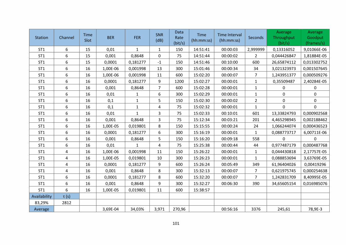
04/set/17

AWGN 7,14E-05 12,13% 676 0,3338 52,28%

POOR 5,26E-05 8,63% 315 0,1552 51,48%

GOOD 2,90E-05 5,09% 107 0,0516 50,98%

Field Test 3,69E-04 34,03% 246 0,0789 83,29%

Algorithm: Trinder

with ACOS 05/set/17

AWGN 3,26E-05 5,91% 1625 0,8047 84,40%

POOR 1,21E-04 14,84% 1041 0,5035 93,76%

GOOD 2,53E-04 27,09% 415 0,1937 79,22%

Field Test 1,82E-04 18,49% 1509 0,6988 86,38%

Algorithm: Trinder

with BEO 07/set/17

AWGN 3,26E-05 5,75% 901 0,3857 95,15%

POOR 4,79E-05 7,71% 372 0,1690 94,42%

GOOD 1,35E-04 16,13% 218 0,0852 83,66%

Field Test 2,68E-04 24,53% 719 0,2283 96,44%

72

73

7. Chapter 7 – Summary and Future Work

This final chapter presents a summary of the developed work and also suggestions for future work

in the HF communications and DRC algorithms.

7.1. Summary

The main objective of this dissertation was to design, implement and test a DRC algorithm with better

performance than the existing solutions, for HF communications, using the E/R GRC-525 military radio.

The development of HF transmissions declined when the satellite communication appeared, as it

allows higher data rates. However, the use of HF band offers more independency and less costs in the

communications section for a nation; in Portugal, satellites are rented to the USA, making it an expensive

system to use. In addition, satellites are vulnerable to physical damage, as it is supported by Earth

infrastructures and, in an emergency, such as an earthquake, satellite communications can be disabled.

In recent years, HF modems and adaptive techniques were developed, allowing high speed modems

(until 9600 bit/s) and renewing the use of HF communications, especially in military situations with hilly

terrain. These communications use the Ionosphere to reflect the sky wave, therefore it is necessary to

know its composition and behaviour.

According to the HF standardisations and the adaptive techniques developed at the beginning of the

millennium, two DRC algorithms were designed, implemented and simulated: Trinder and RapidM DRC

algorithms. Trinder algorithm defines the data rate based on FER thresholds, and RapidM DRC

algorithm updates the data rate according to BER and SNR thresholds.

A simulation system in Matlab was created to assess the original DRC algorithms and detect their

vulnerabilities. After implementing the Trinder and the RapidM DRC algorithms, its main detected

weakness was the data rate oscillations, which lead to many cut-off states, reducing the link availability

and the average throughput and goodput.

In order to increase the performance of the original Trinder and RapidM algorithms, two new versions

of each one were proposed: Avoiding Cut-Off State (ACOS) and Bit Error Optimization (BEO). When

implemented on the simulation environment, these new versions showed huge link performance

improvements relatively to the original versions; however, some data rate oscillations were still detected

in the ACOS based versions.

After assessing all the algorithms in the simulation system, two radio stations, one in Lisbon and

another in Oporto, were assembled. Each station was composed by one E/R GRC-525 military radio

and a RF-1936P dipole antenna. A DRC software application, implementing all the considered DRC

algorithms (original and improved versions) was developed, allowing to assess the algorithms on the

field. The field propagation tests were performed within a period of 9 days, seeking similar propagation

conditions during all the tests. The Ionospheric behaviour and the meteorological conditions were

recorded, since these may justify eventual discrepancies on the results.

The algorithm that showed the best performance results was the RapidM DRC with BEO, increasing

the goodput by 392% and the link availability by 15%, when compared to its original version. It was

expected that the Trinder algorithm with BEO would present similar results, but the day of its test

74

(7th September 2017) coincided with the highest number of Ionospheric warnings and with the worst

average SNR value (3.38 dB). Nonetheless, the Trinder algorithm with BEO exceeded the performance

of its original version, increasing the goodput by 189% and the link availability by 13%. The original

version of Trinder algorithm presented the worst performance results among every tested algorithm.

The HF communications standards used in this dissertation were the STANAG 4539 [24] and the

MIL-STD-118-110B [25].

7.2. Future Work

Despite the good results obtained, showing that the proposed solution allow a significant

improvement of the DRC algorithms original versions, some issues related with HF communications and

the DRC algorithms deserve to be further considered:

Improve the user interface in the DRC application to make it more “user friendly”.

Implementation of the STANAG 5066 in a DRC application.

Design, implement and test an algorithm that changes the frame size according to the

propagation conditions.

75

A. Appendix A – Radio E/R GRC-525 datasheet

76

77

B. Appendix B – Dipole antenna RF-1936P datasheet

78

79

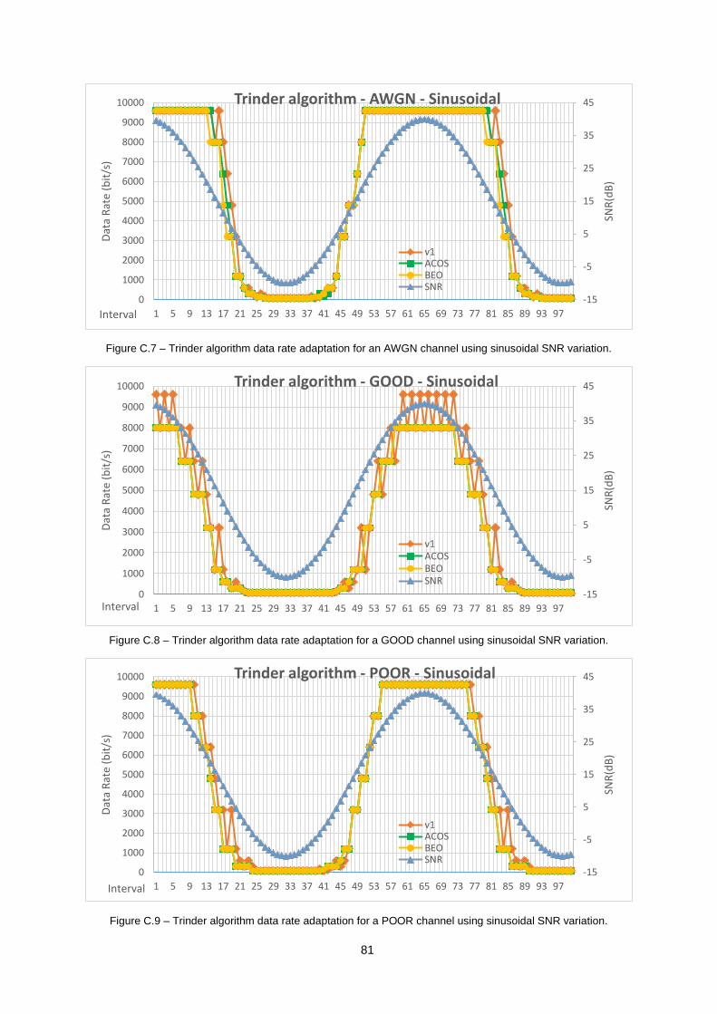
C. Appendix C – Results from Algorithms Assessments

Figure C.1 – Trinder algorithm data rate adaptation for an AWGN channel using downward sinusoidal SNR variation.

Figure C.2 – Trinder algorithm data rate adaptation for a GOOD channel using downward sinusoidal SNR variation.

Figure C.3 - Trinder algorithm data rate adaptation for a POOR channel using downward sinusoidal SNR variation.

-15

-5

5

15

25

35

45

0

1000

2000

3000

4000

5000

6000

7000

8000

9000

10000

1 5 9 13 17 21 25 29 33 37 41 45 49 53 57 61 65 69 73 77 81 85 89 93 97

SNR

(dB

)

Dat

a R

ate

(bit

/s)

Interval

Trinder algorithm - AWGN - Downwardv1

ACOS

BEO

SNR

-15

-5

5

15

25

35

45

0

1000

2000

3000

4000

5000

6000

7000

8000

9000

10000

1 5 9 13 17 21 25 29 33 37 41 45 49 53 57 61 65 69 73 77 81 85 89 93 97SN

R(d

B)

Dat

a R

ate

(bit

/s)

Interval

Trinder algorithm - GOOD - Downwardv1

ACOS

BEO

SNR

-15

-5

5

15

25

35

45

0

1000

2000

3000

4000

5000

6000

7000

8000

9000

10000

1 5 9 13 17 21 25 29 33 37 41 45 49 53 57 61 65 69 73 77 81 85 89 93 97

SNR

(dB

)

Dat

a R

ate

(bit

/s)

Interval

Trinder algorithm - POOR - Downwardv1

ACOS

BEO

SNR

80

Figure C.4 – Trinder algorithm data rate adaptation for an AWGN channel using upward sinusoidal SNR variation.

Figure C.5 – Trinder algorithm data rate adaptation for a GOOD channel using upward sinusoidal SNR variation.

Figure C.6 – Trinder algorithm data rate adaptation for a POOR channel using upward sinusoidal SNR variation.

-15

-5

5

15

25

35

45

0

1000

2000

3000

4000

5000

6000

7000

8000

9000

10000

1 5 9 13 17 21 25 29 33 37 41 45 49 53 57 61 65 69 73 77 81 85 89 93 97

SNR

(dB

)

Dat

a R

ate

(bit

/s)

Interval

Trinder algorithm - AWGN - Upward

v1ACOSBEOSNR

-15

-5

5

15

25

35

45

0

1000

2000

3000

4000

5000

6000

7000

8000

9000

10000

1 5 9 13 17 21 25 29 33 37 41 45 49 53 57 61 65 69 73 77 81 85 89 93 97

SNR

(dB

)

Dat

a R

ate

(bit

/s)

Interval

Trinder algorithm - GOOD - Upward

v1ACOSBEOSNR

-15

-5

5

15

25

35

45

0

1000

2000

3000

4000

5000

6000

7000

8000

9000

10000

1 5 9 13 17 21 25 29 33 37 41 45 49 53 57 61 65 69 73 77 81 85 89 93 97

SNR

(dB

)

Dat

a R

ate

(bit

/s)

Interval

Trinder algorithm - POOR - Upward

v1ACOSBEOSNR

81

Figure C.7 – Trinder algorithm data rate adaptation for an AWGN channel using sinusoidal SNR variation.

Figure C.8 – Trinder algorithm data rate adaptation for a GOOD channel using sinusoidal SNR variation.

Figure C.9 – Trinder algorithm data rate adaptation for a POOR channel using sinusoidal SNR variation.

-15

-5

5

15

25

35

45

0

1000

2000

3000

4000

5000

6000

7000

8000

9000

10000

1 5 9 13 17 21 25 29 33 37 41 45 49 53 57 61 65 69 73 77 81 85 89 93 97

SNR

(dB

)

Dat

a R

ate

(bit

/s)

Interval

Trinder algorithm - AWGN - Sinusoidal

v1ACOSBEOSNR

-15

-5

5

15

25

35

45

0

1000

2000

3000

4000

5000

6000

7000

8000

9000

10000

1 5 9 13 17 21 25 29 33 37 41 45 49 53 57 61 65 69 73 77 81 85 89 93 97SN

R(d

B)

Dat

a R

ate

(bit

/s)

Interval

Trinder algorithm - GOOD - Sinusoidal

v1ACOSBEOSNR

-15

-5

5

15

25

35

45

0

1000

2000

3000

4000

5000

6000

7000

8000

9000

10000

1 5 9 13 17 21 25 29 33 37 41 45 49 53 57 61 65 69 73 77 81 85 89 93 97

SNR

(dB

)

Dat

a R

ate

(bit

/s)

Interval

Trinder algorithm - POOR - Sinusoidal

v1ACOSBEOSNR

82

Figure C.10 – Trinder algorithm data rate adaptation for an AWGN channel using discontinues SNR variation.

Figure C.11 – Trinder algorithm data rate adaptation for a GOOD channel using discontinues SNR variation.

Figure C.12 – Trinder algorithm data rate adaptation for a POOR channel using discontinues SNR variation.

-5

0

5

10

15

20

25

30

0

1000

2000

3000

4000

5000

6000

7000

8000

9000

10000

1 5 9 13 17 21 25 29 33 37 41 45 49 53 57 61 65 69 73 77 81 85 89 93 97

SNR

(dB

)

Dat

a R

ate

(bit

/s)

Interval

Trinder algorithm - AWGN - Discontinuesv1ACOSBEOSNR

-5

0

5

10

15

20

25

30

0

1000

2000

3000

4000

5000

6000

7000

8000

9000

10000

1 5 9 13 17 21 25 29 33 37 41 45 49 53 57 61 65 69 73 77 81 85 89 93 97SN

R(d

B)

Dat

a R

ate

(bit

/s)

Interval

Trinder algorithm - GOOD- Discontinuesv1ACOSBEOSNR

-5

0

5

10

15

20

25

30

0

1000

2000

3000

4000

5000

6000

7000

8000

9000

10000

1 5 9 13 17 21 25 29 33 37 41 45 49 53 57 61 65 69 73 77 81 85 89 93 97

SNR

(dB

)

Dat

a R

ate

(bit

/s)

Interval

Trinder algorithm - POOR- Discontinuesv1ACOSBEOSNR

83

Figure C.13 – RapidM algorithm data rate adaptation for an AWGN channel using downward SNR variation.

Figure C.14 – RapidM algorithm data rate adaptation for a GOOD channel using downward SNR variation.

Figure C.15 – RapidM algorithm data rate adaptation for a POOR channel using downward SNR variation.

-15

-5

5

15

25

35

45

0

1000

2000

3000

4000

5000

6000

7000

8000

9000

10000

1 5 9 13 17 21 25 29 33 37 41 45 49 53 57 61 65 69 73 77 81 85 89 93 97

SNR

(dB

)

Dat

a R

ate

(bit

/s)

Interval

RapidM algorithm - AWGN - Downwardv1ACOSBEOSNR

-15

-5

5

15

25

35

45

0

1000

2000

3000

4000

5000

6000

7000

8000

9000

10000

1 5 9 13 17 21 25 29 33 37 41 45 49 53 57 61 65 69 73 77 81 85 89 93 97SN

R(d

B)

Dat

a R

ate

(bit

/s)

Interval Number

RapidM algorithm - GOOD - Downwardv1ACOSBEOSNR

-15

-5

5

15

25

35

45

0

1000

2000

3000

4000

5000

6000

7000

8000

9000

10000

1 5 9 13 17 21 25 29 33 37 41 45 49 53 57 61 65 69 73 77 81 85 89 93 97

SNR

(dB

)

Dat

a R

ate

(bit

/s)

Interval

RapidM algorithm - POOR - Downwardv1ACOSBEOSNR

84

Figure C.16 – RapidM algorithm data rate adaptation for an AWGN channel using upward SNR variation.

Figure C.17 – RapidM algorithm data rate adaptation for a GOOD channel using upward SNR variation.

Figure C.18 – RapidM algorithm data rate adaptation for a POOR channel using upward SNR variation.

-15

-5

5

15

25

35

45

0

1000

2000

3000

4000

5000

6000

7000

8000

9000

10000

1 5 9 13 17 21 25 29 33 37 41 45 49 53 57 61 65 69 73 77 81 85 89 93 97

SNR

(dB

)

Dat

a R

ate

(bit

/s)

Interval

RapidM algorithm - AWGN - Upward

v1ACOSBEOSNR

-15

-5

5

15

25

35

45

0

1000

2000

3000

4000

5000

6000

7000

8000

9000

10000

1 5 9 13 17 21 25 29 33 37 41 45 49 53 57 61 65 69 73 77 81 85 89 93 97SN

R(d

B)

Dat

a R

ate

(bit

/s)

Interval

RapidM algorithm - GOOD - Upward

v1ACOSBEOSNR

-15

-5

5

15

25

35

45

0

1000

2000

3000

4000

5000

6000

7000

8000

9000

10000

1 5 9 13 17 21 25 29 33 37 41 45 49 53 57 61 65 69 73 77 81 85 89 93 97

SNR

(dB

)

Dat

a R

ate

(bit

/s)

Interval

RapidM algorithm - POOR - Upward

v1ACOSBEOSNR

85

Figure C.19 – RapidM algorithm data rate adaptation for an AWGN channel using sinusoidal SNR variation.

Figure C.20 – RapidM algorithm data rate adaptation for a GOOD channel using sinusoidal SNR variation.

Figure C.21 – RapidM algorithm data rate adaptation for a POOR channel using sinusoidal SNR variation.

-15

-5

5

15

25

35

45

0

1000

2000

3000

4000

5000

6000

7000

8000

9000

10000

1 5 9 13 17 21 25 29 33 37 41 45 49 53 57 61 65 69 73 77 81 85 89 93 97

SNR

(dB

)

Dat

a R

ate

(bit

/s)

Interval

RapidM algorithm - AWGN - Sinusoidal

v1ACOSBEOSNR

-15

-5

5

15

25

35

45

0

1000

2000

3000

4000

5000

6000

7000

8000

9000

10000

1 5 9 13 17 21 25 29 33 37 41 45 49 53 57 61 65 69 73 77 81 85 89 93 97SN

R(d

B)

Dat

a R

ate

(bit

/s)

Interval

RapidM algorithm - GOOD - Sinusoidal

v1ACOSBEOSNR

-15

-5

5

15

25

35

45

0

1000

2000

3000

4000

5000

6000

7000

8000

9000

10000

1 5 9 13 17 21 25 29 33 37 41 45 49 53 57 61 65 69 73 77 81 85 89 93 97

SNR

(dB

)

Dat

a R

ate

(bit

/s)

Interval

RapidM algorithm - POOR - Sinusoidal

v1ACOSBEOSNR

86

Figure C.22 – RapidM algorithm data rate adaptation for an AWGN channel using discontinues SNR variation.

Figure C.23 – RapidM algorithm data rate adaptation for a GOOD channel using discontinues SNR variation.

Figure C.24 – RapidM algorithm data rate adaptation for a POOR channel using discontinues SNR variation.

-5

0

5

10

15

20

25

30

0

1000

2000

3000

4000

5000

6000

7000

8000

9000

10000

1 5 9 13 17 21 25 29 33 37 41 45 49 53 57 61 65 69 73 77 81 85 89 93 97

SNR

(dB

)

Dat

a R

ate

(bit

/s)

Interval

RapidM algorithm - AWGN - Discontinuesv1ACOSBEOSNR

-5

0

5

10

15

20

25

30

0

1000

2000

3000

4000

5000

6000

7000

8000

9000

10000

1 5 9 13 17 21 25 29 33 37 41 45 49 53 57 61 65 69 73 77 81 85 89 93 97SN

R(d

B)

Dat

a R

ate

(bit

/s)

Interval

RapidM algorithm - GOOD - Discontinuesv1ACOSBEOSNR

-5

0

5

10

15

20

25

30

0

1000

2000

3000

4000

5000

6000

7000

8000

9000

10000

1 5 9 13 17 21 25 29 33 37 41 45 49 53 57 61 65 69 73 77 81 85 89 93 97

SNR

(dB

)

Dat

a R

ate

(bit

/s)

Interval

RapidM algorithm - POOR - Discontinuesv1ACOSBEOSNR

87

D. Appendix D – HF Communications Electrical Message

01 – 4 MHz TO 8 MHz / 8//

(Gama de frequências / Nº de frequências)

02 – PERMANENTE//

(Período de utilização das frequências)

03 – NIL//

(Distância e altura necessárias para protecção de serviço)

04 LISBOA/POR/ 38º41’N 9º17’W//

(Local Tx [Nome do local, Código do País e coordenadas geográficas])

05 PORTO/POR/ 41º11’N 8º38’W//

(Local Rx [Nome do local, Código do País e coordenadas geográficas])

06 – FX / 4 / 812//

(Classe Estação. / Serviço / Código da função)

07 – H240 / G8D//

(Largura de Banda / Classe TX)

08 – P /13 DBW//

(Tipo de potência / Valor em dBW [Pot. Máxima do emissor])

09 – OMNIDIRECIONAL/ VERTICAL//

(Ganho da antena /máxima direcção de radiação)

10 – J / 09-17//

(Tipo de horário de operação / hora de começo – hora de fim da operação)

11 – 4 MHZ TO 7 MHz / D / CONTÍNUA//

(Gama de sintonia de sistema, incrementos de sintonia e limitações de sintonia existentes)

12 – D//

(Tipo de operação do circuito)

13 – 29AGO17//

(Data limite para ter as frequências)

14 – A. NIL//

(Características do ar)

B. OPERACIONALIZAÇÃO DOS SISTEMAS RF-1936P-10 HARRIS. //.

(Justificações ou observações)

A finalidade é realizar testes NVIS numa distância considerável e testar uma aplicação de adaptação de débito em condições reais de propagação.

88

89

E. Appendix E – Assembly of the Dipole Antenna 1936P

a) b)

c) d)

e) f)

Figure E.1 – Station assembly on images: a) Unroll the dipole wires; b) Attaching the copper bar to perform the ground of the system; c) Wire that connect the radio with the antenna; d) Fixing the base of the antenna to the ground; e) Hoist the mast of the antenna; f) Stretching the coaxial cable to the radio station.

90

91

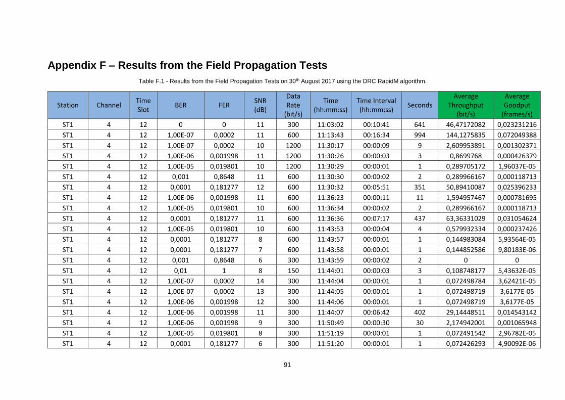
F. Appendix F – Results from the Field Propagation Tests

Table F.1 - Results from the Field Propagation Tests on 30th August 2017 using the DRC RapidM algorithm.

Station Channel Time Slot

BER FER SNR (dB)

Data Rate

(bit/s)

Time (hh:mm:ss)

Time Interval (hh:mm:ss)

Seconds Average

Throughput (bit/s)

Average Goodput

(frames/s)

ST1 4 12 0 0 11 300 11:03:02 00:10:41 641 46,47172082 0,023231216

ST1 4 12 1,00E-07 0,0002 11 600 11:13:43 00:16:34 994 144,1275835 0,072049388

ST1 4 12 1,00E-07 0,0002 10 1200 11:30:17 00:00:09 9 2,609953891 0,001302371

ST1 4 12 1,00E-06 0,001998 11 1200 11:30:26 00:00:03 3 0,8699768 0,000426379

ST1 4 12 1,00E-05 0,019801 10 1200 11:30:29 00:00:01 1 0,289705172 1,96037E-05

ST1 4 12 0,001 0,8648 11 600 11:30:30 00:00:02 2 0,289966167 0,000118713

ST1 4 12 0,0001 0,181277 12 600 11:30:32 00:05:51 351 50,89410087 0,025396233

ST1 4 12 1,00E-06 0,001998 11 600 11:36:23 00:00:11 11 1,594957467 0,000781695

ST1 4 12 1,00E-05 0,019801 10 600 11:36:34 00:00:02 2 0,289966167 0,000118713

ST1 4 12 0,0001 0,181277 11 600 11:36:36 00:07:17 437 63,36331029 0,031054624

ST1 4 12 1,00E-05 0,019801 10 600 11:43:53 00:00:04 4 0,579932334 0,000237426

ST1 4 12 0,0001 0,181277 8 600 11:43:57 00:00:01 1 0,144983084 5,93564E-05

ST1 4 12 0,0001 0,181277 7 600 11:43:58 00:00:01 1 0,144852586 9,80183E-06

ST1 4 12 0,001 0,8648 6 300 11:43:59 00:00:02 2 0 0

ST1 4 12 0,01 1 8 150 11:44:01 00:00:03 3 0,108748177 5,43632E-05

ST1 4 12 1,00E-07 0,0002 14 300 11:44:04 00:00:01 1 0,072498784 3,62421E-05

ST1 4 12 1,00E-07 0,0002 13 300 11:44:05 00:00:01 1 0,072498719 3,6177E-05

ST1 4 12 1,00E-06 0,001998 12 300 11:44:06 00:00:01 1 0,072498719 3,6177E-05

ST1 4 12 1,00E-06 0,001998 11 300 11:44:07 00:06:42 402 29,14448511 0,014543142

ST1 4 12 1,00E-06 0,001998 9 300 11:50:49 00:00:30 30 2,174942001 0,001065948

ST1 4 12 1,00E-05 0,019801 8 300 11:51:19 00:00:01 1 0,072491542 2,96782E-05

ST1 4 12 0,0001 0,181277 6 300 11:51:20 00:00:01 1 0,072426293 4,90092E-06

92


BER FER SNR (dB)

Data Rate

(bit/s)

Time (hh:mm:ss)


Seconds Average

Throughput (bit/s)

Average Goodput

(frames/s)

ST1 4 12 0,001 0,8648 5 150 11:51:21 00:00:02 2 0 0

ST1 4 12 0,01 1 4 75 11:51:23 00:09:52 592 0 0

ST1 4 13 0,01 1 -4 75 12:01:15 00:00:09 9 0,163105969 6,67759E-05

ST1 4 13 0,0001 0,181277 8 75 12:01:24 00:00:01 1 0,01812468 9,04424E-06

ST1 4 13 1,00E-06 0,001998 7 75 12:01:25 00:00:02 2 0,036249396 1,81247E-05

ST1 4 13 0 0 6 150 12:01:27 00:00:01 1 0,03624936 1,80885E-05

ST1 4 13 1,00E-06 0,001998 5 150 12:01:28 00:00:01 1 0,03624936 1,80885E-05

ST1 4 13 1,00E-06 0,001998 4 150 12:01:29 00:00:01 1 0,036245771 1,48391E-05

ST1 4 13 0,0001 0,181277 3 150 12:01:30 00:00:03 3 0,108737313 4,45173E-05

ST1 4 13 0,0001 0,181277 2 150 12:01:33 00:00:44 44 0 0

ST1 2 13 0,01 1 -9 75 12:02:17 00:00:01 1 0 0

ST1 2 13 0,1 1 -8 75 12:02:18 00:00:20 20 0 0

ST1 3 13 0,01 1 -3 75 12:02:38 00:00:03 3 0 0

ST1 3 13 0,01 1 -4 75 12:02:41 00:00:02 2 0 0

ST1 3 13 0,01 1 -5 75 12:02:43 00:00:01 1 0 0

ST1 3 13 0,1 1 -6 75 12:02:44 00:00:17 17 0,308089053 0,000126132

ST1 4 13 0,0001 0,181277 1 75 12:03:01 00:00:01 1 0,018122885 7,41955E-06

ST1 4 13 0,0001 0,181277 3 75 12:03:02 00:00:01 1 0,018124517 8,8829E-06

ST1 4 13 1,00E-05 0,019801 5 75 12:03:03 00:00:01 1 0,018124698 9,06235E-06

ST1 4 13 0 0 8 150 12:03:04 00:00:01 1 0,036249033 1,77658E-05

ST1 4 13 1,00E-05 0,019801 7 150 12:03:05 00:00:03 3 0,108737313 4,45173E-05

ST1 4 13 0,0001 0,181277 6 150 12:03:08 00:01:31 91 3,298691723 0,001646052

ST1 4 13 1,00E-06 0,001998 11 150 12:04:39 00:00:02 2 0,072498784 3,62421E-05

ST1 4 13 1,00E-07 0,0002 10 300 12:04:41 00:07:19 439 31,82665128 0,015598375

ST1 4 13 1,00E-05 0,019801 8 300 12:12:00

93

Availability τ (s)

83,88% 3471

Average 5,08E-06 0,89% 9,501 392,64 01:08:58 4138 379,60 188,3E-3

Table F.2 – Results from the Field Propagation Tests on 31st August 2017 using the DRC RapidM algorithm with ACOS.


BER FER SNR (dB)

Data Rate

(bit/s)

Time (hh:mm:ss)


Seconds Average

Throughput (bit/s)

Average Goodput

(frames/s)

ST1 2 12 0 0 1 75 11:18:40 00:00:04 4 0,094250714 4,71254E-05

ST1 2 12 0 0 0 150 11:18:44 00:00:11 11 0,518378891 0,000259189

ST1 3 12 0 0 -10 75 11:18:55 00:00:04 4 0,094250699 4,71253E-05

ST1 3 12 0 0 -9 75 11:18:59 00:00:02 2 0,04712535 2,35627E-05

ST1 3 12 0 0 -8 75 11:19:01 00:00:06 6 0,141376064 7,0688E-05

ST1 4 12 0 0 9 300 11:19:07 00:00:02 2 0,188501399 9,42507E-05

ST1 4 12 0 0 7 300 11:19:09 00:00:02 2 0,188499573 9,23844E-05

ST1 4 12 1,00E-05 0,019801 6 300 11:19:11 00:00:01 1 0,094249727 4,61922E-05

ST1 4 12 1,00E-05 0,019801 5 300 11:19:12 00:00:01 1 0,094249786 4,61922E-05

ST1 4 12 1,00E-05 0,019801 4 300 11:19:13 00:00:01 1 0,094241304 3,85826E-05

ST1 4 12 0,0001 0,181277 2 300 11:19:14 00:00:02 2 0,188499514 9,23844E-05

ST1 4 12 1,00E-05 0,019801 4 300 11:19:16 00:01:55 115 10,83883128 0,005419416

ST1 4 12 0 0 19 1200 11:21:11 00:00:04 4 1,508011426 0,000754006

ST1 4 12 0 0 18 3200 11:21:15 00:00:02 2 2,010681384 0,00100514

ST1 4 12 1,00E-07 0,0002 17 4800 11:21:17 00:00:08 8 12,06396982 0,005912602

ST1 4 12 1,00E-05 0,019801 14 4800 11:21:25 00:00:57 57 85,87068822 0,005810666

ST1 6 12 0,001 0,8648 8 3200 11:22:22 00:00:03 3 0 0

ST1 6 12 0,01 1 7 1200 11:22:25 00:00:01 1 0,376625676 2,54854E-05

ST1 6 12 0,001 0,8648 6 600 11:22:26 00:02:18 138 26,01319254 0,013003997

ST1 4 12 1,00E-07 0,0002 13 1200 11:24:44 00:00:41 41 15,45710053 0,007713116

ST1 4 12 1,00E-06 0,001998 11 1200 11:25:25 00:00:35 35 13,19496702 0,006466909

94


BER FER SNR (dB)

Data Rate

(bit/s)

Time (hh:mm:ss)


Seconds Average

Throughput (bit/s)

Average Goodput

(frames/s)

ST1 4 12 1,00E-05 0,019801 11 1200 11:26:00 00:00:02 2 0,75400484 0,00037625

ST1 4 12 1,00E-06 0,001998 11 1200 11:26:02 00:07:37 457 172,2902749 0,086127919

ST1 4 12 1,00E-07 0,0002 14 3200 11:33:39 00:00:10 10 10,05340755 0,005025699

ST1 4 12 1,00E-07 0,0002 13 4800 11:33:49 00:00:01 1 1,507860861 0,000617322

ST1 4 12 0,0001 0,181277 11 4800 11:33:50 00:00:02 2 3,013006355 0,000203883

ST1 4 12 0,001 0,8648 9 3200 11:33:52 00:00:01 1 0 0

ST1 4 12 0,01 1 8 1200 11:33:53 00:07:53 473 178,3045052 0,072998261

ST1 4 12 0,0001 0,181277 7 1200 11:41:46 00:00:01 1 0,376625676 2,54854E-05

ST1 4 12 0,001 0,8648 6 600 11:41:47 00:00:03 3 0 0

ST1 4 12 0,01 1 5 300 11:41:50 00:00:01 1 0,094241304 3,85826E-05

ST1 4 12 0,0001 0,181277 8 300 11:41:51 00:00:01 1 0,094250635 4,70312E-05

ST1 4 12 1,00E-06 0,001998 11 300 11:41:52 00:05:57 357 33,64749898 0,016820387

ST1 4 12 1,00E-07 0,0002 9 600 11:47:49 00:00:03 3 0,565504198 0,000282696

ST1 4 12 1,00E-07 0,0002 8 1200 11:47:52 00:00:01 1 0,376998909 0,000184769

ST1 4 12 1,00E-05 0,019801 9 1200 11:47:53 00:00:01 1 0,376965215 0,00015433

ST1 4 12 0,0001 0,181277 8 1200 11:47:54 00:00:01 1 0,376625913 2,54854E-05

ST1 4 12 0,001 0,8648 7 600 11:47:55 00:00:02 2 0,376625794 2,54854E-05

ST1 4 12 0,001 0,8648 6 300 11:47:57 00:00:02 2 0,188499514 9,23844E-05

ST1 4 12 1,00E-05 0,019801 8 300 11:47:59 00:00:01 1 0,094250719 4,71159E-05

ST1 4 12 1,00E-07 0,0002 11 600 11:48:00 00:00:03 3 0,565504198 0,000282696

ST1 4 12 1,00E-07 0,0002 10 1200 11:48:03 00:09:16 556 209,5926107 0,085807681

ST1 4 12 0,0001 0,181277 9 1200 11:57:19 00:00:05 5 1,88312909 0,000127427

ST1 4 12 0,001 0,8648 8 600 11:57:24 00:00:01 1 0,188312956 1,27427E-05

ST1 4 12 0,001 0,8648 6 300 11:57:25 00:00:01 1 0,094241245 3,85826E-05

ST1 4 12 0,0001 0,181277 5 300 11:57:26 00:00:02 2 0,188312956 1,27427E-05

ST1 4 12 0,001 0,8648 4 150 11:57:28 00:00:01 1 0 0

95


BER FER SNR (dB)

Data Rate

(bit/s)

Time (hh:mm:ss)


Seconds Average

Throughput (bit/s)

Average Goodput

(frames/s)

ST1 4 12 0,01 1 3 75 11:57:29 00:00:01 1 0 0

ST1 4 12 0,1 1 2 75 11:57:30 00:00:02 2 0 0

ST1 4 12 0,1 1 1 75 11:57:32 00:00:01 1 0 0

ST1 4 12 0,01 1 0 75 11:57:33 00:00:04 4 0,094156449 6,37134E-06

ST1 4 12 0,001 0,8648 -1 75 11:57:37 00:01:47 107 2,521203885 0,001258085

ST1 6 12 1,00E-06 0,001998 6 75 11:59:24 00:00:01 1 0,023562447 1,15481E-05

ST1 6 12 1,00E-05 0,019801 5 75 11:59:25 00:00:01 1 0,023560326 9,64565E-06

ST1 6 12 0,0001 0,181277 4 75 11:59:26 00:00:01 1 0,023560311 9,64564E-06

ST1 6 12 0,0001 0,181277 3 75 11:59:27 00:00:01 1 0,02353912 1,59284E-06

ST1 6 12 0,001 0,8648 2 75 11:59:28 00:00:02 2 0,047120637 1,92913E-05

ST1 6 12 0,0001 0,181277 5 75 11:59:30 00:00:06 6 0,141361926 5,78739E-05

ST1 7 12 0,0001 0,181277 3 75 11:59:36 00:00:01 1 0,023560326 9,64565E-06

ST1 7 12 0,0001 0,181277 5 75 11:59:37 00:00:01 1 0,023560311 9,64564E-06

ST1 7 12 0,0001 0,181277 4 75 11:59:38 00:00:02 2 0,047078224 3,18567E-06

ST1 7 12 0,001 0,8648 3 75 11:59:40 00:00:02 2 0 0

ST1 7 12 0,01 1 2 75 11:59:42 00:00:01 1 0 0

ST1 7 12 0,01 1 1 75 11:59:43 00:00:02 2 0 0

ST1 7 12 0,1 1 0 75 11:59:45 00:00:05 5 0 0

ST1 7 12 0,1 1 -1 75 11:59:50 00:00:09 9 0,212042874 8,68108E-05

ST1 8 12 0,0001 0,181277 4 75 11:59:59 00:00:03 3 0,070680963 2,89369E-05

ST1 8 12 0,0001 0,181277 3 75 12:00:02 00:00:02 2 0,047078239 3,18567E-06

ST1 8 12 0,001 0,8648 2 75 12:00:04 00:00:04 4 0 0

ST1 8 12 0,01 1 1 75 12:00:08 00:00:30 30 0,706873235 0,000346442

ST1 4 13 1,00E-05 0,019801 7 75 12:00:38 00:00:01 1 0,023560311 9,64564E-06

ST1 4 13 0,0001 0,181277 5 75 12:00:39 00:00:02 2 0,047120652 1,92913E-05

ST1 4 13 0,0001 0,181277 4 75 12:00:41 00:00:01 1 0,023560311 9,64564E-06

96


BER FER SNR (dB)

Data Rate

(bit/s)

Time (hh:mm:ss)


Seconds Average

Throughput (bit/s)

Average Goodput

(frames/s)

ST1 4 13 0,0001 0,181277 3 75 12:00:42 00:00:01 1 0,02353912 1,59284E-06

ST1 4 13 0,001 0,8648 1 75 12:00:43 00:00:02 2 0,047078224 3,18567E-06

ST1 4 13 0,001 0,8648 0 75 12:00:45 00:01:20 80 0 0

ST1 4 13 0,01 1 -1 75 12:02:05 00:00:02 2 0 0

ST1 4 13 0,1 1 -2 75 12:02:07 00:00:01 1 0 0

ST1 4 13 0,1 1 -1 75 12:02:08 00:00:02 2 0 0

ST1 4 13 0,1 1 -2 75 12:02:10 00:00:01 1 0 0

ST1 4 13 0,1 1 -1 75 12:02:11 00:00:01 1 0 0

ST1 4 13 0,01 1 0 75 12:02:12 00:00:01 1 0,023560326 9,64565E-06

ST1 4 13 0,0001 0,181277 5 75 12:02:13 00:00:01 1 0,023560311 9,64564E-06

ST1 4 13 0,0001 0,181277 4 75 12:02:14 00:00:02 2 0,047078224 3,18567E-06

ST1 4 13 0,001 0,8648 3 75 12:02:16 00:00:03 3 0 0

ST1 4 13 0,01 1 2 75 12:02:19 00:00:09 9 0,212063884 0,00010582

ST1 6 13 1,00E-06 0,001998 11 300 12:02:28 00:00:01 1 0,094250719 4,71159E-05

ST1 6 13 1,00E-07 0,0002 14 600 12:02:29 00:00:03 3 0,56550408 0,000282696

ST1 6 13 1,00E-07 0,0002 13 1200 12:02:32 00:00:02 2 0,754005077 0,00037625

ST1 6 13 1,00E-06 0,001998 12 1200 12:02:34 00:00:06 6 2,2619944 0,001108613

ST1 7 13 1,00E-05 0,019801 8 1200 12:02:40 00:00:02 2 0,753930194 0,000308661

ST1 7 13 0,0001 0,181277 7 1200 12:02:42 00:00:01 1 0,376625676 2,54854E-05

ST1 7 13 0,001 0,8648 6 600 12:02:43 00:00:01 1 0,188499573 9,23844E-05

ST1 7 13 1,00E-05 0,019801 9 600 12:02:44 00:00:03 3 0,565503689 0,000282187

ST1 7 13 1,00E-06 0,001998 8 600 12:02:47 00:00:02 2 0,377002759 0,000188464

ST1 7 13 1,00E-07 0,0002 11 1200 12:02:49 00:00:13 13 0 0

ST1 8 13 0,01 1 3 600 12:03:02 00:00:01 1 0,188312956 1,27427E-05

ST1 8 13 0,001 0,8648 4 300 12:03:03 00:00:01 1 0,094241304 3,85826E-05

ST1 8 13 0,0001 0,181277 5 300 12:03:04 00:00:04 4 0,376625794 2,54854E-05

97


BER FER SNR (dB)

Data Rate

(bit/s)

Time (hh:mm:ss)


Seconds Average

Throughput (bit/s)

Average Goodput

(frames/s)

ST1 8 13 0,001 0,8648 4 150 12:03:08 00:00:03 3 0,141361926 5,78739E-05

ST1 8 13 0,0001 0,181277 3 150 12:03:11 00:00:31 31 1,460739854 0,00059803

ST1 4 13 0,0001 0,181277 3 150 12:03:42 00:00:01 1 0,047124893 2,30961E-05

ST1 4 13 1,00E-05 0,019801 8 150 12:03:43 00:00:01 1 0,047125364 2,35627E-05

ST1 4 13 0 0 12 300 12:03:44 00:00:03 3 0,282752127 0,000141376

ST1 4 13 0 0 15 600 12:03:47 00:07:41 461 86,89914299 0,043440887

ST1 4 13 1,00E-07 0,0002 14 1200 12:11:28 00:00:09 9 3,393025191 0,001696173

ST1 4 13 1,00E-07 0,0002 13 3200 12:11:37 00:00:01 1 1,005330423 0,000492717

ST1 4 13 1,00E-05 0,019801 11 3200 12:11:38 00:00:01 1 1,005331055 0,000492717

ST1 4 13 1,00E-05 0,019801 10 3200 12:11:39 00:00:01 1 1,005240574 0,000411548

ST1 4 13 0,0001 0,181277 8 3200 12:11:40 00:00:01 1 1,004335136 6,7961E-05

ST1 4 13 0,001 0,8648 7 1200 12:11:41 00:00:02 2 0,754005077 0,00037625

ST1 4 13 1,00E-06 0,001998 8 1200 12:11:43

Availability τ (s)

95,95% 3054

Average 6,69E-05 9,26% 9,328 904,44 00:53:03 3183 892,22 369,0E-3

Table F.3 – Results from the Field Propagation Tests on 1st September 2017 using the DRC RapidM algorithm with BEO.


BER FER SNR (dB)

Data Rate

(bit/s)

Time (hh:mm:ss)


Seconds Average

Throughput (bit/s)

Average Goodput

(frames/s)

ST1 4 10 0 0 -3 75 09:43:09 00:00:01 1 0,02300614 1,15031E-05

ST1 4 10 0 0 -2 150 09:43:10 00:00:02 2 0,092024532 4,60123E-05

ST1 4 10 0 0 1 300 09:43:12 00:00:02 2 0,184049065 9,20245E-05

ST1 4 10 0 0 0 300 09:43:14 00:00:01 1 0,092024561 4,60123E-05

98


BER FER SNR (dB)

Data Rate

(bit/s)

Time (hh:mm:ss)


Seconds Average

Throughput (bit/s)

Average Goodput

(frames/s)

ST1 4 10 0 0 -1 300 09:43:15 00:00:01 1 0,092024561 4,60123E-05

ST1 4 10 0 0 0 300 09:43:16 00:00:02 2 0,184049065 9,20245E-05

ST1 4 10 0 0 -1 300 09:43:18 00:00:03 3 0,27607335 0,000137761

ST1 4 10 1,00E-06 0,001998 8 1200 09:43:21 00:00:50 50 18,38650297 0,001244171

ST1 2 10 0,001 0,8648 -7 150 09:44:11 00:00:05 5 0,230038339 9,41782E-05

ST1 2 10 0,0001 0,181277 -3 150 09:44:16 00:00:07 7 0,321763821 2,1773E-05

ST1 3 10 0,001 0,8648 -7 75 09:44:23 00:00:02 2 0,045966254 3,11043E-06

ST1 3 10 0,001 0,8648 -6 75 09:44:25 00:00:02 2 0,045966254 3,11043E-06

ST1 3 10 0,001 0,8648 -7 75 09:44:27 00:00:02 2 0 0

ST1 3 10 0,01 1 -8 75 09:44:29 00:03:21 201 4,619608892 0,000312598

ST1 3 10 0,001 0,8648 -5 75 09:47:50 00:00:06 6 0 0

ST1 3 10 0,01 1 -6 75 09:47:56 00:00:02 2 0 0

ST1 3 10 0,1 1 -5 75 09:47:58 00:00:05 5 0,115030661 5,75038E-05

ST1 3 10 1,00E-07 0,0002 8 300 09:48:03 00:00:11 11 1,012269843 0,000506034

ST1 7 10 1,00E-07 0,0002 11 600 09:48:14 00:00:01 1 0,184048989 9,20061E-05

ST1 7 10 1,00E-07 0,0002 14 1200 09:48:15 00:00:01 1 0,368098209 0,000184012

ST1 7 10 1,00E-07 0,0002 15 3200 09:48:16 00:00:02 2 1,963188063 0,000979634

ST1 7 10 1,00E-06 0,001998 14 3200 09:48:18 00:10:07 607 595,822263 0,292014987

ST1 7 10 1,00E-05 0,019801 12 3200 09:58:25 00:02:04 124 121,7176698 0,0607373

ST1 7 10 1,00E-06 0,001998 14 3200 10:00:29 00:00:01 1 0,981584888 0,000481079

ST1 7 10 1,00E-05 0,019801 14 3200 10:00:30 00:00:01 1 0,981585506 0,000481079

ST1 7 10 1,00E-05 0,019801 13 3200 10:00:31 00:00:01 1 0,981496545 0,000401827

ST1 7 10 0,0001 0,181277 11 3200 10:00:32 00:00:01 1 0,981497162 0,000401827

ST1 7 10 0,0001 0,181277 10 3200 10:00:33 00:00:01 1 0,980613726 6,63558E-05

ST1 7 11 0,001 0,8648 8 1200 10:00:34 00:00:06 6 2,208566693 0,001082428

ST1 7 11 1,00E-05 0,019801 7 1200 10:00:40 00:00:03 3 1,104293401 0,000551044

99


BER FER SNR (dB)

Data Rate

(bit/s)

Time (hh:mm:ss)


Seconds Average

Throughput (bit/s)

Average Goodput

(frames/s)

ST1 7 11 1,00E-06 0,001998 11 1200 10:00:43 00:00:47 47 17,29888355 0,007082201

ST1 2 11 0,0001 0,181277 -4 150 10:01:30 00:00:01 1 0,046011792 2,25506E-05

ST1 2 11 1,00E-05 0,019801 -1 150 10:01:31 00:00:01 1 0,046011821 2,25506E-05

ST1 2 11 1,00E-05 0,019801 -2 150 10:01:32 00:00:03 3 0,138035433 6,76517E-05

ST1 2 11 1,00E-05 0,019801 -3 150 10:01:35 00:00:03 3 0,138023009 5,65069E-05

ST1 2 11 0,0001 0,181277 -4 150 10:01:38 00:00:13 13 0 0

ST1 3 11 0,01 1 -10 75 10:01:51 00:00:04 4 0 0

ST1 3 11 0,01 1 -8 75 10:01:55 00:00:08 8 0,184049079 9,20245E-05

ST1 4 11 0 0 14 300 10:02:03 00:00:01 1 0,092024504 4,60123E-05

ST1 4 11 0 0 17 600 10:02:04 00:00:04 4 0,736196302 0,000368025

ST1 4 11 1,00E-07 0,0002 16 1200 10:02:08 00:00:01 1 0,368097977 0,000184012

ST1 4 11 1,00E-07 0,0002 15 3200 10:02:09 00:00:01 1 0,981595223 0,0004907

ST1 4 11 1,00E-07 0,0002 14 4800 10:02:10 00:09:57 597 879,0096147 0,430806294

ST1 4 11 1,00E-05 0,019801 13 4800 10:12:07 00:00:11 11 16,18012278 0,001094871

ST1 4 11 0,001 0,8648 12 3200 10:12:18 00:00:03 3 2,9447559 0,001443237

ST1 4 11 1,00E-05 0,019801 11 3200 10:12:21 00:09:43 583 571,6976686 0,038685426

ST1 4 11 0,001 0,8648 9 1200 10:22:04 00:00:05 5 1,840306716 0,000753426

ST1 4 11 0,0001 0,181277 8 1200 10:22:09 00:00:04 4 1,472378027 0,000721619

ST1 4 11 1,00E-05 0,019801 11 1200 10:22:13 00:00:05 5 1,84047236 0,000902023

ST1 4 11 1,00E-05 0,019801 10 1200 10:22:18 00:00:30 30 11,04184053 0,004520554

ST1 7 11 0,0001 0,181277 10 1200 10:22:48 00:00:05 5 1,840306716 0,000753426

ST1 7 11 0,0001 0,181277 8 1200 10:22:53 00:00:43 43 15,82663803 0,006479461

ST1 2 11 0,0001 0,181277 -5 150 10:23:36 00:00:05 5 0,230038339 9,41782E-05

ST1 2 11 0,0001 0,181277 -6 150 10:23:41 00:00:41 41 1,886501188 0,000941367

ST1 4 11 1,00E-06 0,001998 9 600 10:24:22 00:00:02 2 0,368097762 0,000183681

ST1 4 11 1,00E-06 0,001998 8 600 10:24:24 00:12:56 776 142,8206576 0,069997003

100


BER FER SNR (dB)

Data Rate

(bit/s)

Time (hh:mm:ss)


Seconds Average

Throughput (bit/s)

Average Goodput

(frames/s)

ST1 4 11 1,00E-05 0,019801 6 600 10:37:20 00:00:01 1 0,184047282 9,02023E-05

ST1 4 11 1,00E-05 0,019801 5 600 10:37:21 00:00:01 1 0,184030718 7,53426E-05

ST1 4 11 0,0001 0,181277 4 600 10:37:22 00:00:03 3 0,5521467 0,000275522

ST1 4 11 1,00E-06 0,001998 8 600 10:37:25 00:00:01 1 0,184048989 9,20061E-05

ST1 4 11 1,00E-07 0,0002 11 1200 10:37:26 00:00:02 2 0,736188898 0,000360809

ST1 4 11 1,00E-05 0,019801 9 1200 10:37:28 00:00:01 1 0,368094565 0,000180405

ST1 4 11 1,00E-05 0,019801 8 1200 10:37:29

Availability τ (s)

99,17% 3233

Average 2,76E-04 24,98% 9,548 2426,79 00:54:20 3260 2425,23 927,1E-3

Table F.4 – Results from the Field Propagation Tests on 4th September 2017 using the Trinder algorithm.


BER FER SNR (dB)

Data Rate

(bit/s)

Time (hh:mm:ss)


Seconds Average

Throughput (bit/s)

Average Goodput

(frames/s)

ST1 6 15 0 0 5 150 14:42:41 00:00:10 10 0,444312816 0,000222156

ST1 7 15 0 0 2 300 14:42:51 00:00:01 1 0,088862524 4,44313E-05

ST1 7 15 0 0 1 600 14:42:52 00:00:02 2 0,35509487 2,40284E-05

ST1 7 15 0,001 0,8648 0 300 14:42:54 00:00:01 1 0,088853638 3,63769E-05

ST1 7 15 0,0001 0,181277 -1 600 14:42:55 00:00:02 2 0,355094758 2,40284E-05

ST1 7 15 0,001 0,8648 0 300 14:42:57 00:00:01 1 0,088861691 4,35515E-05

ST1 7 15 1,00E-05 0,019801 2 600 14:42:58 00:08:33 513 91,16386846 0,03732269

ST1 7 15 0,0001 0,181277 1 1200 14:51:31 00:00:08 8 2,840758288 0,000192227

ST1 6 15 0,001 0,8648 4 600 14:51:39 00:00:01 1 0,177547435 1,20142E-05

ST1 6 15 0,001 0,8648 3 300 14:51:40 00:00:01 1 0 0

101


BER FER SNR (dB)

Data Rate

(bit/s)

Time (hh:mm:ss)


Seconds Average

Throughput (bit/s)

Average Goodput

(frames/s)

ST1 6 15 0,01 1 1 150 14:51:41 00:00:03 2,999999 0,13316052 9,01066E-06

ST1 6 15 0,001 0,8648 0 75 14:51:44 00:00:02 2 0,044426847 1,81884E-05

ST1 6 15 0,0001 0,181277 -1 150 14:51:46 00:10:00 600 26,65874112 0,013302752

ST1 6 16 1,00E-06 0,001998 13 300 15:01:46 00:00:34 34 3,021323973 0,001507645

ST1 6 16 1,00E-06 0,001998 11 600 15:02:20 00:00:07 7 1,243951377 0,000509276

ST1 6 16 0,0001 0,181277 9 1200 15:02:27 00:00:01 1 0,35509487 2,40284E-05

ST1 6 16 0,001 0,8648 7 600 15:02:28 00:00:01 1 0 0

ST1 6 16 0,01 1 6 300 15:02:29 00:00:01 1 0 0

ST1 6 16 0,1 1 5 150 15:02:30 00:00:02 2 0 0

ST1 6 16 0,1 1 4 75 15:02:32 00:00:01 1 0 0

ST1 6 16 0,01 1 3 75 15:02:33 00:10:01 601 13,33824793 0,000902568

ST1 6 16 0,001 0,8648 3 75 15:12:34 00:03:21 201 4,465298945 0,002188462

ST1 6 16 1,00E-05 0,019801 8 150 15:15:55 00:00:24 24 1,066244074 0,000436523

ST1 6 16 0,0001 0,181277 6 300 15:16:19 00:00:01 1 0,088773717 6,00711E-06

ST1 6 16 0,001 0,8648 5 150 15:16:20 00:09:18 558 0 0

ST1 6 16 0,01 1 4 75 15:25:38 00:00:44 44 0,977487179 0,000487768

ST1 4 16 1,00E-06 0,001998 11 150 15:26:22 00:00:01 1 0,044430818 2,17757E-05

ST1 4 16 1,00E-05 0,019801 10 300 15:26:23 00:00:01 1 0,088853694 3,63769E-05

ST1 4 16 0,0001 0,181277 9 600 15:26:24 00:05:49 349 61,96404026 0,00419296

ST1 4 16 0,001 0,8648 8 300 15:32:13 00:00:07 7 0,621975745 0,000254638

ST1 6 16 0,0001 0,181277 8 600 15:32:20 00:00:07 7 1,242831709 8,40995E-05

ST1 6 16 0,001 0,8648 9 300 15:32:27 00:06:30 390 34,65605154 0,016985076

ST1 6 16 1,00E-05 0,019801 11 600 15:38:57

Availability τ (s)

83,29% 2812

Average 3,69E-04 34,03% 3,971 270,96 00:56:16 3376 245,61 78,9E-3

102

Table F.5 – Results from the Field Propagation Tests on 5th September 2017 using the Trinder algorithm with ACOS.


BER FER SNR (dB)

Data Rate

(bit/s)

Time (hh:mm:ss)


Seconds Average

Throughput (bit/s)

Average Goodput

(frames/s)

ST1 4 13 0 0 8 300 12:06:40 00:00:09 9 1,138268577 0,00055787

ST1 4 13 1,00E-05 0,019801 8 600 12:06:49 00:03:51 231 58,43111887 0,028637336

ST1 4 13 1,00E-05 0,019801 7 1200 12:10:40 00:00:02 2 1,011703123 0,000414194

ST1 4 13 0,0001 0,181277 6 3200 12:10:42 00:00:02 2 2,69544751 0,000182395

ST1 4 13 0,001 0,8648 5 1200 12:10:44 00:00:02 2 1,011703123 0,000414194

ST1 4 13 0,0001 0,181277 4 1200 12:10:46 00:00:02 2 1,010792499 6,83979E-05

ST1 4 13 0,001 0,8648 3 600 12:10:48 00:00:05 5 1,263490703 8,54974E-05

ST1 4 13 0,001 0,8648 2 300 12:10:53 00:00:01 1 0,12646293 5,17742E-05

ST1 4 13 0,0001 0,181277 1 600 12:10:54 00:00:01 1 0,252925701 0,000103548

ST1 4 13 0,0001 0,181277 0 600 12:10:55 00:04:09 249 62,92183821 0,004257772

ST1 4 13 0,001 0,8648 1 300 12:15:04 00:00:03 3 0,379422859 0,000185957

ST1 4 13 1,00E-05 0,019801 2 600 12:15:07 00:05:21 321 81,18918202 0,033239032

ST1 4 13 0,0001 0,181277 0 600 12:20:28 00:00:01 1 0,252698204 1,70995E-05

ST1 4 13 0,001 0,8648 -1 300 12:20:29 00:00:03 3 0,379388711 0,000155323

ST1 4 13 0,0001 0,181277 -2 300 12:20:32 00:00:01 1 0,126349102 8,54974E-06

ST1 4 13 0,001 0,8648 -3 150 12:20:33 00:00:01 1 0 0

ST1 4 13 0,01 1 -4 75 12:20:34 00:00:02 2 0,063237137 3,09928E-05

ST1 4 13 1,00E-05 0,019801 -5 150 12:20:36 00:01:27 87 5,501631338 0,002696373

ST1 4 13 1,00E-05 0,019801 0 300 12:22:03 00:00:02 2 0,252925781 0,000103548

ST1 4 13 0,0001 0,181277 1 600 12:22:05 00:00:01 1 0,252698204 1,70995E-05

ST1 4 13 0,001 0,8648 2 300 12:22:06 00:00:02 2 0,252925781 0,000103548

ST1 4 13 0,0001 0,181277 1 600 12:22:08 00:00:04 4 1,010792658 6,83979E-05

ST1 4 13 0,001 0,8648 0 300 12:22:12 00:00:03 3 0 0

ST1 4 13 0,01 1 -1 150 12:22:15 00:00:11 11 0,695614783 0,000347113

103


BER FER SNR (dB)

Data Rate

(bit/s)

Time (hh:mm:ss)


Seconds Average

Throughput (bit/s)

Average Goodput

(frames/s)

ST1 6 13 1,00E-06 0,001998 7 300 12:22:26 00:00:01 1 0,126475451 6,31114E-05

ST1 6 13 1,00E-06 0,001998 6 600 12:22:27 00:00:02 2 0,505851561 0,000207097

ST1 6 13 0,0001 0,181277 5 1200 12:22:29 00:00:03 3 1,517554843 0,00062129

ST1 6 13 0,0001 0,181277 8 3200 12:22:32 00:00:06 6 0 0

ST1 7 13 0,01 1 2 1200 12:22:38 00:00:04 4 0 0

ST1 7 13 0,01 1 1 600 12:22:42 00:00:02 2 0 0

ST1 7 13 0,01 1 -1 300 12:22:44 00:00:01 1 0,126349023 8,54974E-06

ST1 7 13 0,001 0,8648 -2 150 12:22:45 00:00:03 3 0,189694355 7,76613E-05

ST1 7 13 0,0001 0,181277 -3 300 12:22:48 00:00:01 1 0 0

ST1 7 13 0,1 1 -4 150 12:22:49 00:01:32 92 0 0

ST1 7 13 0,01 1 -5 75 12:24:21 00:00:02 2 0,063174531 4,27487E-06

ST1 7 13 0,001 0,8648 -6 75 12:24:23 00:00:09 9 0,284541533 0,000116492

ST1 7 13 0,0001 0,181277 -3 150 12:24:32 00:00:28 28 1,770655879 0,00088356

ST1 8 13 1,00E-06 0,001998 4 300 12:25:00 00:00:01 1 0,126474313 6,19856E-05

ST1 8 13 1,00E-05 0,019801 5 600 12:25:01 00:00:02 2 0,505897092 0,000247942

ST1 8 13 1,00E-05 0,019801 8 1200 12:25:03 00:01:30 90 0 0

ST1 4 13 0,01 1 -1 600 12:26:33 00:00:02 2 0,505396249 3,4199E-05

ST1 4 13 0,001 0,8648 -2 300 12:26:35 00:00:01 1 0,126349102 8,54974E-06

ST1 4 13 0,001 0,8648 -3 150 12:26:36 00:00:05 5 0,315872676 2,13744E-05

ST1 4 13 0,001 0,8648 -2 75 12:26:41 00:00:03 3 0,094855715 4,64892E-05

ST1 4 13 1,00E-05 0,019801 -1 150 12:26:44 00:00:12 12 0,758853191 0,000379351

ST1 6 13 1,00E-07 0,0002 8 300 12:26:56 00:00:01 1 0,126475565 6,32251E-05

ST1 6 13 1,00E-07 0,0002 7 600 12:26:57 00:00:01 1 0,252950743 0,000126223

ST1 6 13 1,00E-06 0,001998 8 1200 12:26:58 00:00:04 4 2,023588688 0,000991769

ST1 6 13 1,00E-05 0,019801 7 3200 12:27:02 00:00:06 6 0 0

ST1 7 13 0,1 1 -3 1200 12:27:08 00:00:02 2 0 0

104


BER FER SNR (dB)

Data Rate

(bit/s)

Time (hh:mm:ss)


Seconds Average

Throughput (bit/s)

Average Goodput

(frames/s)

ST1 7 13 0,1 1 -4 600 12:27:10 00:00:02 2 0 0

ST1 7 13 0,1 1 -5 300 12:27:12 00:00:19 19 2,403033015 0,001199117

ST1 8 13 1,00E-06 0,001998 7 600 12:27:31 00:00:01 1 0,252948626 0,000123971

ST1 8 13 1,00E-05 0,019801 6 1200 12:27:32 00:00:01 1 0,50539609 3,4199E-05

ST1 8 13 0,001 0,8648 4 600 12:27:33 00:00:01 1 0,252698204 1,70995E-05

ST1 8 13 0,001 0,8648 3 300 12:27:34 00:00:01 1 0,126349102 8,54974E-06

ST1 8 13 0,001 0,8648 2 150 12:27:35 00:00:03 2,999999 0,18971139 9,29783E-05

ST1 8 13 1,00E-05 0,019801 1 300 12:27:38 00:00:34 34 4,300164385 0,002145788

ST1 6 13 1,00E-06 0,001998 6 600 12:28:12 00:00:01 1 0,252948467 0,000123971

ST1 6 13 1,00E-05 0,019801 5 1200 12:28:13 00:01:24 84 0 0

ST1 4 13 0,01 1 -1 600 12:29:37 00:00:01 1 0 0

ST1 4 13 0,01 1 -2 300 12:29:38 00:00:02 2 0,252698125 1,70995E-05

ST1 4 13 0,001 0,8648 -3 150 12:29:40 00:00:01 1 0,063174551 4,27487E-06

ST1 4 13 0,001 0,8648 -4 75 12:29:41 00:00:02 2 0,063231445 2,58871E-05

ST1 4 13 0,0001 0,181277 -5 150 12:29:43 00:00:03 3 0,189694355 7,76613E-05

ST1 4 13 0,0001 0,181277 -1 300 12:29:46 00:00:03 3 0,379422859 0,000185957

ST1 4 13 1,00E-05 0,019801 0 300 12:29:49 00:00:11 11 1,391217124 0,000681841

ST1 6 13 1,00E-05 0,019801 4 600 12:30:00 00:00:01 1 0,252925701 0,000103548

ST1 6 13 0,0001 0,181277 3 600 12:30:01 00:00:01 1 0,25292586 0,000103548

ST1 6 13 0,0001 0,181277 2 600 12:30:02 00:00:01 1 0,252698204 1,70995E-05

ST1 6 13 0,001 0,8648 1 300 12:30:03 00:00:01 1 0,126462851 5,17742E-05

ST1 6 13 0,0001 0,181277 0 300 12:30:04 00:00:07 7 0 0

ST1 7 13 0,01 1 -4 150 12:30:11 00:00:01 1 0,063174511 4,27487E-06

ST1 7 13 0,001 0,8648 -3 75 12:30:12 00:00:02 2 0,063231445 2,58871E-05

ST1 7 13 0,0001 0,181277 -1 150 12:30:14 00:00:05 5,000001 0,315872715 2,13744E-05

ST1 7 13 0,001 0,8648 -2 75 12:30:19 00:00:05 5 0,158078623 6,47177E-05

105


BER FER SNR (dB)

Data Rate

(bit/s)

Time (hh:mm:ss)


Seconds Average

Throughput (bit/s)

Average Goodput

(frames/s)

ST1 7 13 0,0001 0,181277 -1 150 12:30:24 00:00:08 8 0,505897132 0,000247942

ST1 6 13 1,00E-05 0,019801 1 300 12:30:32 00:00:02 2 0,252925781 0,000103548

ST1 6 13 0,0001 0,181277 0 300 12:30:34 00:01:34 94 11,88858263 0,005826644

ST1 4 13 1,00E-05 0,019801 0 300 12:32:08 00:00:03 3 0,379047227 2,56492E-05

ST1 4 13 0,001 0,8648 -2 150 12:32:11 00:00:09 9 0,56913998 0,00028457

ST1 6 13 0 0 9 300 12:32:20 00:00:01 1 0,126475498 6,32377E-05

ST1 6 13 0 0 12 600 12:32:21 00:00:02 2 0,505902101 0,0002529

ST1 6 13 1,00E-07 0,0002 11 1200 12:32:23 00:00:02 2 1,01180452 0,000505801

ST1 6 13 1,00E-07 0,0002 10 3200 12:32:25 00:00:02 2 2,698117826 0,001322359

ST1 6 13 1,00E-05 0,019801 9 3200 12:32:27 00:00:01 1 1,347723755 9,11973E-05

ST1 6 13 0,001 0,8648 8 1200 12:32:28 00:00:01 1 0,505896933 0,000247942

ST1 6 13 1,00E-05 0,019801 7 3200 12:32:29 00:00:01 1 1,347723755 9,11973E-05

ST1 6 13 0,001 0,8648 6 1200 12:32:30 00:00:03 3 1,517554843 0,00062129

ST1 6 13 0,0001 0,181277 5 1200 12:32:33 00:00:10 10 0 0

ST1 7 13 0,01 1 -1 600 12:32:43 00:00:01 1 0 0

ST1 7 13 0,01 1 -2 300 12:32:44 00:00:02 2 0,252698125 1,70995E-05

ST1 7 13 0,001 0,8648 -3 75 12:32:46 00:00:02 2 0,063231445 2,58871E-05

ST1 7 13 0,0001 0,181277 -4 150 12:32:48 00:00:07 7 0,442660016 0,00021695

ST1 8 13 1,00E-05 0,019801 1 300 12:32:55 00:00:01 1 0,126462851 5,17742E-05

ST1 8 13 0,0001 0,181277 0 300 12:32:56 00:00:02 2 0,252698125 1,70995E-05

ST1 8 13 0,001 0,8648 -1 150 12:32:58 00:00:02 2 0,126349102 8,54974E-06

ST1 8 13 0,001 0,8648 -2 75 12:33:00 00:00:01 1 0,031618843 1,57778E-05

ST1 8 13 1,00E-06 0,001998 0 150 12:33:01 00:00:03 3 0,189694355 7,76613E-05

ST1 8 13 0,0001 0,181277 -1 300 12:33:04 00:00:05 5 0,631745351 4,27487E-05

ST1 8 13 0,001 0,8648 -2 150 12:33:09 00:00:27 27 1,707402826 0,000836805

ST1 6 13 1,00E-05 0,019801 3 300 12:33:36 00:00:01 1 0,126474313 6,19856E-05

106


BER FER SNR (dB)

Data Rate

(bit/s)

Time (hh:mm:ss)


Seconds Average

Throughput (bit/s)

Average Goodput

(frames/s)

ST1 6 13 1,00E-05 0,019801 2 600 12:33:37 00:00:01 1 0,252698204 1,70995E-05

ST1 6 13 0,001 0,8648 1 300 12:33:38 00:00:01 1 0,126349023 8,54974E-06

ST1 6 13 0,001 0,8648 0 150 12:33:39 00:00:01 1 0,063174551 4,27487E-06

ST1 6 13 0,001 0,8648 -1 75 12:33:40 00:00:01 1 0,031618558 1,54964E-05

ST1 6 13 1,00E-05 0,019801 -2 150 12:33:41 00:00:02 2 0,126349102 8,54974E-06

ST1 6 13 0,001 0,8648 -3 75 12:33:43 00:00:04 4 0,126474273 6,19856E-05

ST1 6 13 1,00E-05 0,019801 -4 150 12:33:47 00:01:24 84 5,311441831 0,002174516

ST1 4 13 0,0001 0,181277 -2 300 12:35:11 00:00:01 1 0,126349102 8,54974E-06

ST1 4 13 0,001 0,8648 -3 150 12:35:12 00:00:02 2 0 0

ST1 4 13 0,01 1 -4 75 12:35:14 00:00:01 1 0,031587276 2,13744E-06

ST1 4 13 0,001 0,8648 -5 75 12:35:15 00:00:06 6 0,189694335 7,76613E-05

ST1 4 13 0,0001 0,181277 -3 150 12:35:21 00:00:01 1 0,063237156 3,09928E-05

ST1 4 13 1,00E-05 0,019801 0 300 12:35:22 00:00:12 12 1,517706534 0,000758853

ST1 6 13 0 0 11 600 12:35:34 00:00:02 2 0,505901805 0,000252446

ST1 6 13 1,00E-06 0,001998 10 1200 12:35:36 00:00:01 1 0,505896933 0,000247942

ST1 6 13 1,00E-05 0,019801 9 3200 12:35:37 00:00:03 3 4,047177164 0,001983538

ST1 6 13 1,00E-05 0,019801 14 4800 12:35:40 00:00:07 7 0 0

ST1 7 13 0,1 1 -5 3200 12:35:47 00:00:01 1 0 0

ST1 7 13 0,1 1 -3 1200 12:35:48 00:00:01 1 0 0

ST1 7 13 0,1 1 1 600 12:35:49 00:00:02 2 0,505396249 3,4199E-05

ST1 7 13 0,001 0,8648 3 300 12:35:51 00:00:02 2 0,252925781 0,000103548

ST1 7 13 0,0001 0,181277 4 600 12:35:53 00:00:05 5,000001 1,26474297 0,000619856

ST1 7 13 1,00E-05 0,019801 8 1200 12:35:58 00:00:11 11 5,564923269 0,002781905

ST1 8 13 1,00E-07 0,0002 14 3200 12:36:09 00:00:01 1 1,349059337 0,00066118

ST1 8 13 1,00E-05 0,019801 15 4800 12:36:10 00:10:02 602 1218,200297 0,597045068

ST1 8 13 1,00E-05 0,019801 14 6400 12:46:12

107

Availability τ (s)

86,38% 2049

Average 1,82E-04 18,49% 4,980 1645,87 00:39:32 2372 1508,52 698,8E-3

Table F.6 – Results from the Field Propagation Tests on 7th September 2017 using the Trinder algorithm with BEO.


BER FER SNR (dB)

Data Rate

(bit/s)

Time (hh:mm:ss)


Seconds Average

Throughput (bit/s)

Average Goodput

(frames/s)

ST1 6 15 0 0 -1 75 14:42:32 00:00:02 2 0,055066075 2,7533E-05

ST1 6 15 0 0 0 150 14:42:34 00:00:01 1 0,055066087 2,75275E-05

ST1 6 15 1,00E-07 0,0002 1 300 14:42:35 00:04:03 243 26,76208773 0,013354322

ST1 6 15 1,00E-06 0,001998 1 600 14:46:38 00:03:21 201 44,2687004 0,018123704

ST1 6 15 0,0001 0,181277 0 300 14:49:59 00:00:06 6 0,66078636 0,000323854

ST1 6 15 1,00E-05 0,019801 -1 300 14:50:05 00:00:01 1 0,110121171 4,50839E-05

ST1 6 15 0,0001 0,181277 -3 150 14:50:06 00:00:05 5 0,275055061 1,86123E-05

ST1 6 15 0,001 0,8648 -4 75 14:50:11 00:00:01 1 0,027532771 1,34939E-05

ST1 6 15 1,00E-05 0,019801 -5 150 14:50:12 00:00:56 56 3,083700434 0,00154185

ST1 4 15 0 0 9 300 14:51:08 00:00:01 1 0,110132104 5,5055E-05

ST1 4 15 1,00E-07 0,0002 7 600 14:51:09 00:00:01 1 0,220264148 0,000109912

ST1 4 15 1,00E-06 0,001998 5 1200 14:51:10 00:00:03 3 1,321453776 0,000541006

ST1 4 15 0,0001 0,181277 3 600 14:51:13 00:01:21 81 17,83962557 0,007303582

ST1 4 15 0,0001 0,181277 1 300 14:52:34 00:00:01 1 0,110131014 5,39757E-05

ST1 4 15 1,00E-05 0,019801 0 300 14:52:35 00:00:01 1 0,110121171 4,50839E-05

ST1 4 15 0,0001 0,181277 -2 150 14:52:36 00:00:21 21 0 0

ST1 6 15 0,01 1 -6 75 14:52:57 00:00:06 6 0,165181722 6,76258E-05

ST1 6 15 0,0001 0,181277 -5 75 14:53:03 00:00:07 7 0,192731078 9,61731E-05

ST1 7 15 1,00E-06 0,001998 0 150 14:53:10 00:00:02 2 0,110132074 5,49561E-05

ST1 7 15 1,00E-06 0,001998 1 300 14:53:12 00:00:01 1 0,110131014 5,39757E-05

108


BER FER SNR (dB)

Data Rate

(bit/s)

Time (hh:mm:ss)


Seconds Average

Throughput (bit/s)

Average Goodput

(frames/s)

ST1 7 15 1,00E-05 0,019801 2 600 14:53:13 00:00:02 2 0,440524332 0,000215903

ST1 7 15 1,00E-05 0,019801 3 600 14:53:15 00:00:03 2,999999 0,660792168 0,000329736

ST1 7 15 1,00E-06 0,001998 4 600 14:53:18 00:14:15 855 188,325803 0,093974858

ST1 7 16 1,00E-06 0,001998 5 1200 15:07:33 00:00:10 10 4,405242213 0,002159028

ST1 6 16 1,00E-05 0,019801 8 3200 15:07:43 00:00:01 1 1,173567819 7,94126E-05

ST1 6 16 0,001 0,8648 6 1200 15:07:44 00:00:01 1 0,440484684 0,000180335

ST1 6 16 0,0001 0,181277 4 600 15:07:45 00:00:01 1 0,220242342 9,01677E-05

ST1 6 16 0,0001 0,181277 2 300 15:07:46 00:00:01 1 0,110131014 5,39757E-05

ST1 6 16 1,00E-05 0,019801 4 600 15:07:47 00:00:01 1 0,220262166 0,000107951

ST1 6 16 1,00E-05 0,019801 6 1200 15:07:48 00:08:42 522 229,7259912 0,015545013

ST1 6 16 0,001 0,8648 -2 600 15:16:30 00:00:14 14 3,080616769 0,000208458

ST1 6 16 0,001 0,8648 -3 300 15:16:44 00:01:12 72 0 0

ST1 3 16 0,1 1 -10 150 15:17:56 00:00:12 12 0,660792933 0,000330396

ST1 4 16 0 0 7 300 15:18:08 00:00:01 1 0,110132173 5,50551E-05

ST1 4 16 1,00E-07 0,0002 6 600 15:18:09 00:00:01 1 0,220262166 0,000107951

ST1 4 16 1,00E-05 0,019801 5 1200 15:18:10 00:00:03 3 1,321453776 0,000541006

ST1 4 16 0,0001 0,181277 4 600 15:18:13 00:00:02 2 0,440524194 0,000215903

ST1 4 16 1,00E-05 0,019801 3 600 15:18:15 00:00:02 2 0,440528158 0,000219824

ST1 4 16 1,00E-06 0,001998 8 1200 15:18:17 00:05:02 302 133,0383173 0,065202637

ST1 4 16 1,00E-05 0,019801 6 1200 15:23:19 00:01:50 110 48,4096916 0,003275769

ST1 4 16 0,001 0,8648 0 600 15:25:09 00:00:12 12 2,64052856 0,000178678

ST1 6 16 0,001 0,8648 -1 300 15:25:21 00:00:03 3 0,330066087 2,23348E-05

ST1 6 16 0,001 0,8648 -2 150 15:25:24 00:01:33 93 5,121094183 0,00250987

ST1 4 16 1,00E-05 0,019801 -1 300 15:26:57 00:00:01 1 0,110131014 5,39757E-05

ST1 4 16 1,00E-05 0,019801 -2 300 15:26:58 00:00:01 1 0,110121171 4,50839E-05

ST1 4 16 0,0001 0,181277 -3 150 15:26:59 00:00:01 1 0,055011026 3,72247E-06

109


BER FER SNR (dB)

Data Rate

(bit/s)

Time (hh:mm:ss)


Seconds Average

Throughput (bit/s)

Average Goodput

(frames/s)

ST1 4 16 0,001 0,8648 -4 75 15:27:00 00:00:01 1 0,027505496 1,86123E-06

ST1 4 16 0,001 0,8648 -5 75 15:27:01 00:00:02 2 0 0

ST1 4 16 0,01 1 -6 75 15:27:03 00:00:02 2 0 0

ST1 4 16 0,1 1 -7 75 15:27:05 00:00:16 16 0,440524228 0,000215903

ST1 6 16 1,00E-05 0,019801 -2 150 15:27:21 00:00:01 1 0,055065507 2,69878E-05

ST1 6 16 1,00E-05 0,019801 -3 150 15:27:22 00:00:01 1 0,055060586 2,25419E-05

ST1 6 16 0,0001 0,181277 -4 75 15:27:23 00:00:15 15 0,412991457 0,000202409

ST1 7 16 1,00E-05 0,019801 -3 150 15:27:38 00:00:02 2 0,110121171 4,50839E-05

ST1 7 16 0,0001 0,181277 -5 75 15:27:40 00:00:16 16 0,440528633 0,000220264

ST1 8 16 0 0 9 150 15:27:56

Availability τ (s)

96,44% 2627

Average 2,68E-04 24,53% 3,383 728,432 00:45:24 2724 718,94 228,3E-3

110

111

G. Appendix G – Ionospheric Conditions for the Test Days

a) b)

Figure G.1 – Ionospheric conditions for the 30th August 2017: a) foF2 real measure in red colour, and foF2 predicted value in white colour during the day; b) MUF values during the day.

a) b)

Figure G.2 – Ionospheric conditions for the 31st August 2017: a) foF2 real measure in red colour, and foF2 predicted value in white colour during the day; b) MUF values during the day.

a) b)

Figure G.3 – Ionospheric conditions for the 1st September 2017: a) foF2 real measure in red colour, and foF2 predicted value in white colour during the day; b) MUF values during the day.

112

a) b)

Figure G.4 – Ionospheric conditions for the 4th September 2017: a) foF2 real measure in red colour, and foF2 predicted value in white colour during the day; b) MUF values during the day.

a) b)

Figure G.5 – Ionospheric conditions for the 5th September 2017: a) foF2 real measure in red colour, and foF2 predicted value in white colour during the day; b) MUF values during the day.

a) b)

Figure G.6– Ionospheric conditions for the 7th September 2017: a) foF2 real measure in red colour, and foF2 predicted value in white colour during the day; b) MUF values during the day.

113

Bibliography

[1] S. Saraç, F. Kara and C. Vural, “Real-Time Implementation of STANAG 4539 High-Speed HF

Model,” International Journal of Social, Behavioural, Educational, Economic, Business, and

Industrial Engineering, vol. 6, pp. 1289-1294, 2012.

[2] Empresa de Investigação e Desenvolvimento de Electrónica, S.A., Rádio Táctico HF/VHF/UHF

TR-525, Manual de Operação e Manutenção Nível I, Ed. 4 ed.

[3] S. Schulze and G. P. Hancke, Design and Implementation of a STANAG 5066 Data Rate Change

Algorithm for High Data Rate Autobaud Waveforms, Lynnwood Road, Pretoria, 0002, South Africa:

Department of Electrical, Electronic and Computer Engineering, University of Pretoria , 2005.

[4] Wikipédia, “Link Quality Analysis,” 15 August 2012. [Online]. Available:

https://en.wikipedia.org/wiki/Link_quality_analysis. [Accessed 8 November 2016].

[5] Wikipedia, “Automatic Link Establishment,” 16 November 2016. [Online]. Available:

https://en.wikipedia.org/wiki/Automatic_link_establishment. [Accessed 19 November 2016].

[6] S. Trinder and A. Gillespie, “Optimisation of the STANAG 5066 ARQ Protocol to Support High

Data Rate HF Communication,” in Proceedings of IEEE Military Communications Conference

(MILCOM) 2001, Washington, DC, October 2001.

[7] E. E. Johnson, E. Koski, W. N. Furman, M. Jorgenson and J. Nieto, Third-Generation and

Wideband HF Radio Communications, 685 Canton Street Norwood MA 02062: Artech House,

2013.

[8] “Science Pole,” [Online]. Available: http://sciencepole.com/radio-spectrum/#. [Accessed 8 October

2016].

[9] K. Davies, Ionospheric Radio, Peter Peregrinus Ltd, 1990.

[10] Wikipédia, “Ionosphere,” 5 December 2016. [Online]. Available:

https://en.wikipedia.org/wiki/Ionosphere. [Accessed 21 December 2016].

[11] D. Bilitza, International Reference Ionosphere, Radio Science , 2001.

[12] J. K. Hargreaves, The Solar-Terrestrial Environment, Cambridge University Press, 1995.

[13] Wikipedia, “Ionosphere Layers,” 11 November 2015. [Online]. Available:

http://wiki.robotz.com/index.php/Ionosphere_Layers. [Accessed 27 December 2016].

[14] J. J. Carr, Practical Antenna Handbook, 4º ed., McGraw-Hill, 2001.

[15] T. R. Rocha, Comunicações Tácticas e de Emergência por propagação por efeito NVIS, Instituto

Superior Técnico; Academia Militar, 2013.

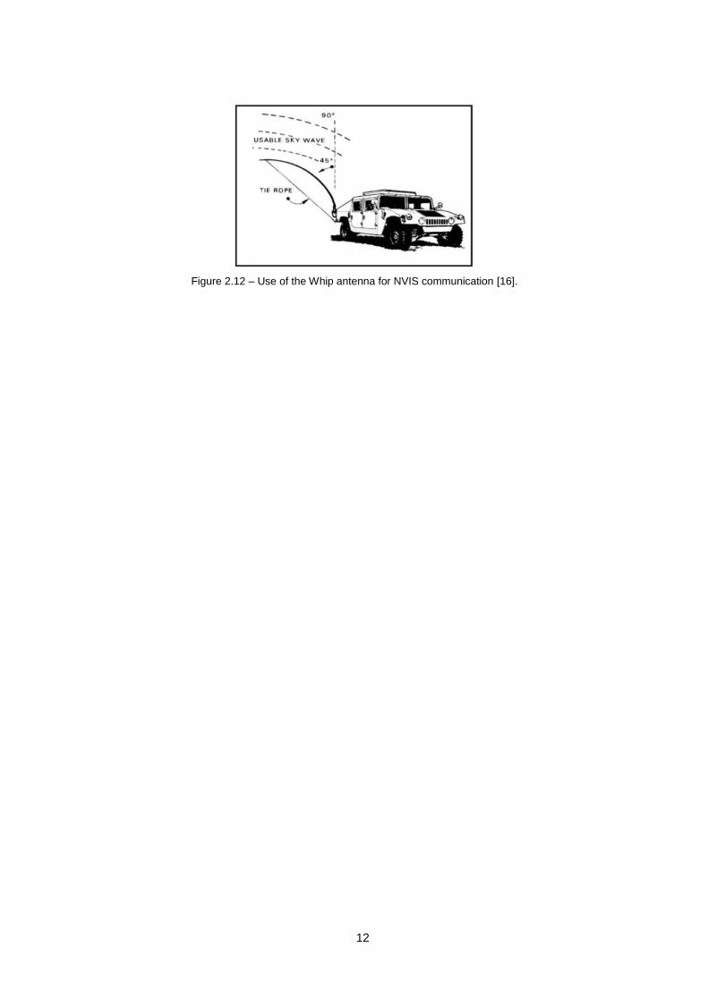
[16] C. P. Grifo, Relatório de Avaliação do Emprego Operacional do E/R GRC-525 na banda HF,

Calçada da Ajuda 134, 1349-053 Lisboa: Direcção de Comunicações e Sistemas de Informação,

Exército Português, Ministério da Defesa Nacional, 2014.

114

[17] AMSAT-CT, “Associação Observatório AeroEspacial Amadores de Satélite - CT,” [Online].

Available: http://www.amsat-ct.pt/?page_id=1221. [Accessed 17 July 2017].

[18] R. Matyszkiel, P. Kaniewski and B. Grochowina, Selected issues of modern HF communications,

05-130 Zegrze Pld, Warszawska 22 A str., Poland: Military Communication Institute, 2013.

[19] Raynet HF Team, “Propagation: What is NVIS?,” 2016. [Online]. Available: http://raynet-

hf.net/propagation/. [Accessed 21 December 2016].

[20] Wikipedia, “Critical Frequency,” 6 August 2016. [Online]. Available:

https://en.wikipedia.org/wiki/Critical_frequency. [Accessed 13 November 2016].

[21] T. A. Ceita, Estudo Comparativo entre duas Antenas para Comunicação com Efeito NVIS, Lisboa:

Instituto Superior Técnico, Academia Militar, 2014.

[22] International Telecommunication Union, Handbook Frequency-Adaptive Communication Systems

and Networks in the MF/HF bands, Place des Nations CH-1211 Geneva 20, Switzerland, 2002.

[23] B. Crystal, “HF Link,” 2007. [Online]. Available: http://hflink.com/alehamradio/. [Accessed 27

December 2016].

[24] STANAG 4539, Technical Standards for Non-Hopping HF Communications Waveforms, NATO,

2000.

[25] MIL-STD-188-110B, Interoperability and Performance Standards for Data Modems, Department

of Defense United States of America, 2000 .

[26] M. Jorgenson and K. Moreland, HF Serial-Tone Waveform Design, 307 Carling Ave., Ottawa,

Canada, K2H 8S2: Communications Research Centre , 1999 .

[27] Rapid Mobile (Pty) Lda., “RapidM,” 2016. [Online]. Available:

http://www.rapidm.com/standard.shtml. [Accessed 4 December 2016].

[28] International Telecomunication Union, Draft Modification of Recommendation ITU-R F.763-4: Data

transmission over HF circuits using phase shift keying or quadrature amplitude modulation, 2004.

[29] M. Carlsen, Adaptive Coding and ModulationTechniques for HF Communication, Trondheim,

Norway: Norwegian University of Science and Technology , 2009.

[30] S. Trinder and D. Brown, Algorithms for the Adapation of Data Rate using STANAG 5066, London,

United Kingdom: IEE Colloquium on Frequency Selection and Management Techniques, 1999.

[31] J. Nieto, An investigation of Throughput Performance for STANAG 5066 High Data Rate HF

Waveforms, Anaheim, CA: Proceedings of IEEE MILCOM 2002, 2002.

[32] C. Salema, Feixes Hertzianos, 3ª ed., Av. Rovisco Pais, Lisbon, Portugal: Instituto Superior

Técnico Press, 2011.

[33] Rohde & Schwarz, GB2 Platform Protocol -M3TR / Series 4100 - Common Part, Munich, Germany:

2GE5, 2008.

[34] Space Weather Prediction Center - National Oceanic and Atmospheric Administration ,

“Geomagnetic Storms,” [Online]. Available: http://www.swpc.noaa.gov/phenomena/geomagnetic-

storms. [Accessed 29 August 2017].

115

[35] Korean Space Weather Center , “Solar flares and HF communication fadeouts,” National Radio

Research Agency, 2011. [Online]. Available:

http://spaceweather.rra.go.kr/effect/english/03_02_02. [Accessed 29 August 2017].

[36] J. Perkiömäki, J. Watson and J. Juopperi, “VOACAP Online,” Voice of America Coverage Analysis

Program, 2010-2017. [Online]. Available: http://www.voacap.com/p2p/index.html. [Accessed 2017

August 2017].

[37] Tutorials Point (I) Pvt. Ltd., C# Programming: Object-Oriented Programming, 3rd Floor, Jyoti

Celestia, Madhapur, Hyderabad, Telangana 500081, India: Tutorials Point - Simply Easy Learning,

2014.

[38] Imapala Multimedia, “Impala News,” [Online]. Available: http://www.impala.pt/. [Accessed 29

August 2017].

Date post:	18-Dec-2018
Category:	Documents
Upload:	vuonghanh
View:	212 times
Download:	0 times

Data Rate Change Algorithms for HF Band Efficient ... · Sergeant 1st Class (OR-7) Mário Arede and...

Documents