38
Database Design Patterns Winter 2006-2007 Lecture 24
| Date post: | 06-May-2018 |
| Category: |
Documents |
| Upload: | hoangtuyen |
| View: | 214 times |
| Download: | 1 times |

Database Design Patterns
Winter 2006-2007Lecture 24

Trees and Hierarchies• Many schemas need to represent trees or
hierarchies of some sort• Common way of representing trees:
– An adjacency list model– Each node in the hierarchy specifies its parent node– Can represent arbitrary tree depths
• Example: employee database– employee(emp_name, address, salary)– manages(emp_name, manager_name)– Both attributes of manages are foreign keys
referencing employee relation
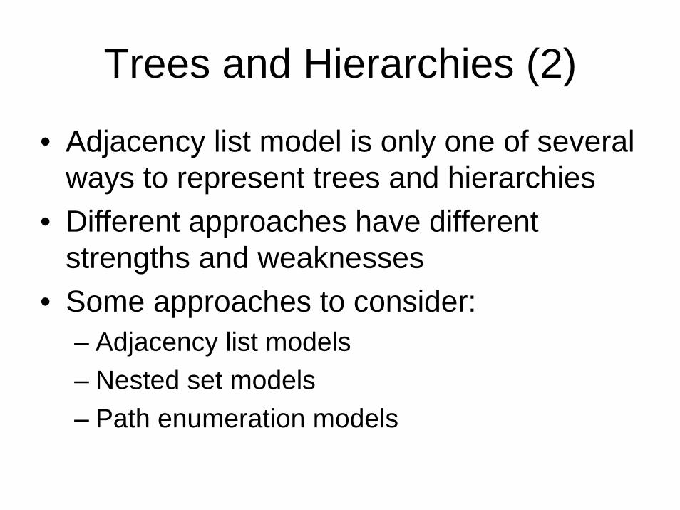
Trees and Hierarchies (2)
• Adjacency list model is only one of several ways to represent trees and hierarchies
• Different approaches have different strengths and weaknesses
• Some approaches to consider:– Adjacency list models– Nested set models– Path enumeration models
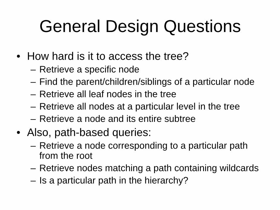
General Design Questions• How hard is it to access the tree?
– Retrieve a specific node– Find the parent/children/siblings of a particular node– Retrieve all leaf nodes in the tree– Retrieve all nodes at a particular level in the tree– Retrieve a node and its entire subtree
• Also, path-based queries:– Retrieve a node corresponding to a particular path
from the root– Retrieve nodes matching a path containing wildcards– Is a particular path in the hierarchy?
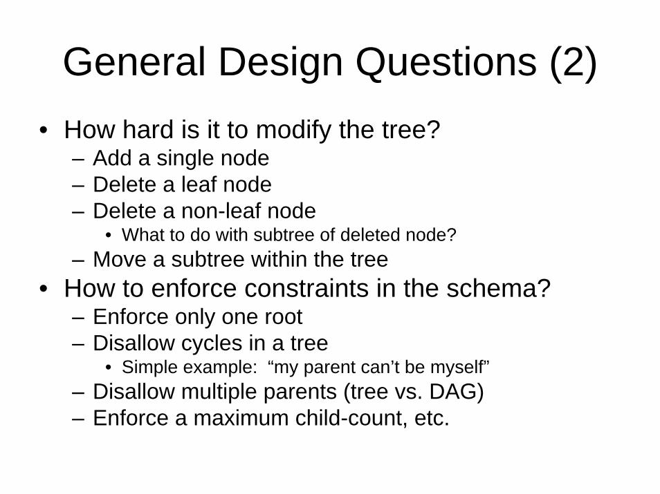
General Design Questions (2)• How hard is it to modify the tree?
– Add a single node– Delete a leaf node– Delete a non-leaf node
• What to do with subtree of deleted node?– Move a subtree within the tree
• How to enforce constraints in the schema?– Enforce only one root– Disallow cycles in a tree
• Simple example: “my parent can’t be myself”– Disallow multiple parents (tree vs. DAG)– Enforce a maximum child-count, etc.
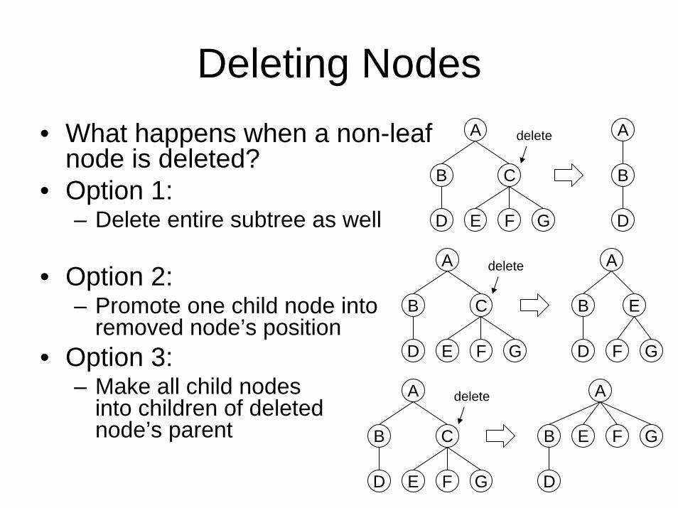
Deleting Nodes• What happens when a non-leaf
node is deleted?• Option 1:
– Delete entire subtree as well
• Option 2:– Promote one child node into
removed node’s position• Option 3:
– Make all child nodesinto children of deletednode’s parent
A
B C
E F GD
A
B
D
delete
A
B C
E F GD
A
B E
F GD
delete
A
B C
E F GD
A
B E F G
D
delete

Adjacency List Model
• Very common approach for modeling trees• Each node specifies its parent node• Relationship between nodes usually
stored in a separate table– e.g. employee and manages– Can represent multiple trees without null
values– Can have employees that are not part of the
hierarchy

Adjacency List Model (2)
• Strengths:– A very flexible model for manipulating trees– Easy to add a new node anywhere in the tree– Easy to move a whole subtree– Deleting a node usually requires extra steps
• Weaknesses:– Operations on entire subtrees are expensive– Operations applied to a particular level across a tree
are expensive– Looking for a node at a specific path is expensive

Queries on Subtrees• Example query using subtrees:
– For every manager reporting to some Vice President, find total number of employees under that manager, and their total salaries
– Computing an aggregate over individual subtrees• Another example:
– Database containing parts in a mechanical assembly• Parts combined into sub-assemblies• Sub-assemblies and parts combined into larger assemblies• Top level assembly is the entire system
– Find number of parts, the total cost, and the total weight of each sub-assembly in the system
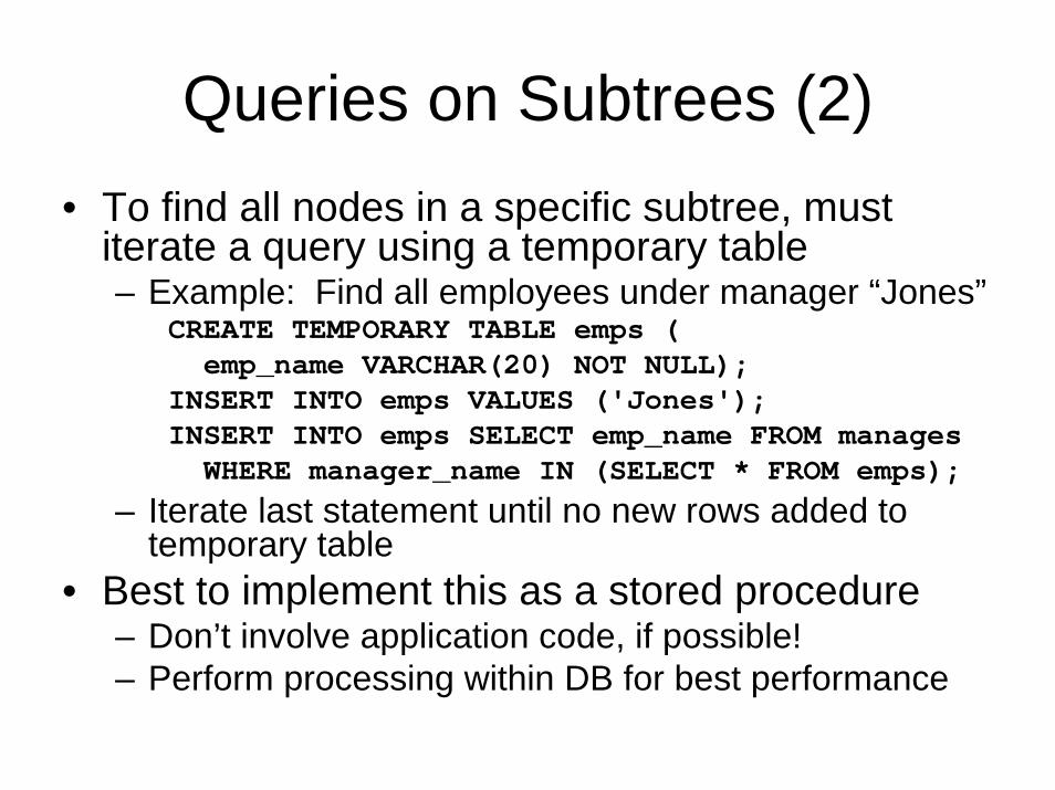
Queries on Subtrees (2)• To find all nodes in a specific subtree, must
iterate a query using a temporary table– Example: Find all employees under manager “Jones”
CREATE TEMPORARY TABLE emps (emp_name VARCHAR(20) NOT NULL);
INSERT INTO emps VALUES ('Jones');INSERT INTO emps SELECT emp_name FROM manages
WHERE manager_name IN (SELECT * FROM emps);– Iterate last statement until no new rows added to
temporary table• Best to implement this as a stored procedure
– Don’t involve application code, if possible!– Perform processing within DB for best performance

Other Adjacency List Notes
• Must manually order siblings under a node– Add another column to the table for ordering
siblings• Adjacency list model is also good for
representing graphs– Actually easier than using for trees, because
less constraints are required– Traversing the graph requires temporary
tables and iterative stored procedures

Nested Set Model• A model optimized for selecting subtrees• Represents hierarchy using containment
– A node “contains” its children• Give each node a “low” and “high” value
– Specifies a range– Always: low < high
• Use this to represent trees:– A parent node’s [low, high] range contains the ranges
of all child nodes– Sibling nodes have non-overlapping ranges
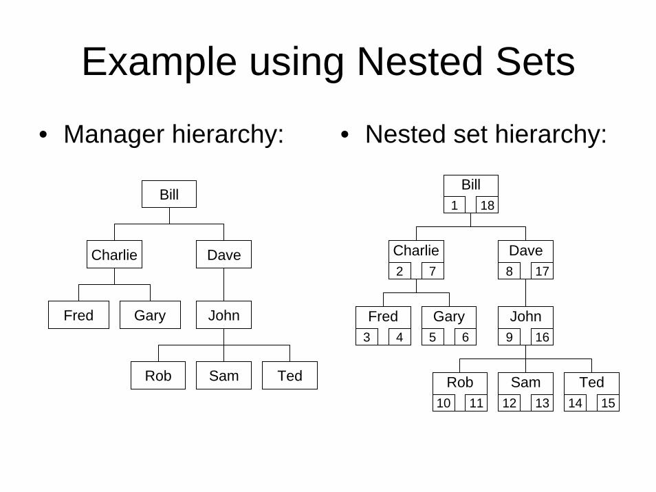
Example using Nested Sets
• Manager hierarchy: • Nested set hierarchy:
Bill181
Fred3 4
Gary5 6
Dave178
Charlie72
John169
Rob1110
Sam1312
Ted1514
Bill
Charlie Dave
Fred Gary John
Rob Sam Ted

Selecting Subtrees• Each parent node contains its children:
• Easy to select an entire subtree– Select all nodes with low (or high) value within node’s range
• Can also select all leaf nodes easily– If all range values separated by 1, find nodes with low + 1 = high– For arbitrary range sizes, find nodes that contain no other node’s
range values (requires self-join)
Fred Gary
Rob Sam Ted
John
DaveCharlie
1
Bill
2 3 4 5 6 7 8 9 10 11 12 13 14 15 16 17 18

Nested Set Model• Strengths:
– Very easy to select a whole subtree• Very important for generating reports against a tree
– Tracking the order of siblings is built in• Weaknesses:
– Some selections are more expensive• e.g. finding all leaf nodes in tree requires self-join
– Constraints on range values are expensive• Needs CHECK constraints
– Pretty costly to insert nodes or restructure trees• Have to update node bounds properly

Adding Nodes In Nested Set Model
• If adding a node:– Must choose range values for new node correctly– Often need to update range values of many other
nodes, even for simple updates• Example:
– Add new employee Harryunder Charlie
– Must update ranges ofmost nodes in the tree!
Bill201
Fred3 4
Gary5 6
Dave1910
Charlie92
John1811
Rob1312
Sam1514
Ted1716
Harry7 8
newnode
Supporting Faster Additions
• Can separate range values by larger amounts– e.g. spacing of 100 instead of 1– Situations requiring range-adjustments of many
nodes will be far less frequent• Can implement tree-manipulation operations as
stored procedures– “Add a node,” “move a subtree,” etc.

Path Enumeration Models• For each node in hierarchy:
– Represent node’s position in hierarchy as the path from the root to that node
– Entire path is stored as a single string value• Node enumeration:
– Each node has some unique ID or name– A path contains the IDs of all nodes between root and
a particular node– If ID values are fixed size, don’t need a delimiter– If ID values are variable size, choose a delimiter that
won’t appear in node IDs or names

Path Enumeration Model (2)• Path enumeration model is fastest when nodes
are retrieved using full path– “Is a specified node in the hierarchy?”– “What are the details for a specified node?”– Adjacency list model and nested set model simply
can’t answer these queries quickly!• Example:
– A database-backed directory service (e.g. LDAP or Microsoft Active Directory)
– Objects and properties form a hierarchy– Properties are accessed using full path names
• “sales.printers.colorprint550.queue”
Strengths and Weaknesses• Optimized for read performance
– Retrieving a specific node using its path is very fast– Retrieving an entire subtree is also pretty fast
• Requires text pattern-matching, but matching a prefix is fast• Example: Find all sales print servers
– Use a condition: path LIKE 'sales.printers.%'
• Adding leaf nodes is fast• Restructuring a tree can be very slow
– Have to reconstruct many paths…• Operations rely on string concatenation and
string manipulation

Edge Enumeration• Paths can enumerate edges instead of nodes
– Each level of path specifies index of node to select• Primary method used in books
– Example:
• Like node enumeration, requires string manipulation for most operations
Edge Enumeration Section Name33.13.23.2.13.2.2…
SQLBackgroundData DefinitionBasic Domain TypesBasic Schema Definition in SQL…

Trees and Hierarchies• Can represent trees and hierarchies in several
different ways– Adjacency list model– Nested set model– Path enumeration model
• Each approach has different strengths– Each is optimized for different kinds of usage
• When designing schemas that require hierarchy– Consider functional and non-functional requirements– Choose a model that best suits the problem

Account Password Management
• Need a database to store user accounts– Username, password, other account details
• How to store a user’s password?• What if database application security is
compromised?– Can attacker get a list of all user passwords?– Can the DB administrator be trusted?
• Is the original password actually required?
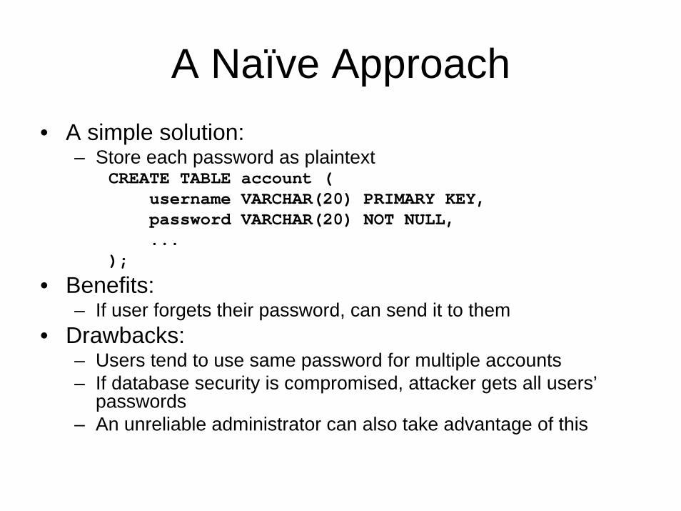
A Naïve Approach• A simple solution:
– Store each password as plaintextCREATE TABLE account (
username VARCHAR(20) PRIMARY KEY,password VARCHAR(20) NOT NULL,...
);
• Benefits:– If user forgets their password, can send it to them
• Drawbacks:– Users tend to use same password for multiple accounts– If database security is compromised, attacker gets all users’
passwords– An unreliable administrator can also take advantage of this

Hashed Passwords• A safer approach is to hash user passwords
– Store hashed password, not the original– For authentication check:
1. User enters password2. Database application hashes the password3. If hash matches value stored in DB, authentication succeeds
• Example using MD5 hash:CREATE TABLE account (
username VARCHAR(20) PRIMARY KEY,pw_hash CHAR(32) NOT NULL,...
);– To store a password:
UPDATE account SET pw_hash = md5('new password')WHERE username = 'joebob';

Hashed Passwords (2)
• Benefits:– Passwords aren’t stored in plaintext anymore
• Drawbacks:– Handling forgotten passwords is trickier
• Need alternate authentication mechanism for users
– Isn’t entirely secure! Still prone to dictionary attacks• Attacker computes dictionary of common
words/names, and their hash value– If attacker gets hash values from database, can crack
some subset of accounts
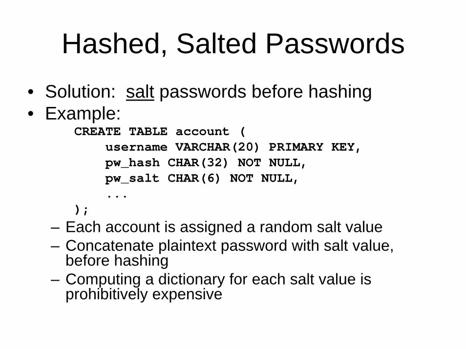
Hashed, Salted Passwords• Solution: salt passwords before hashing• Example:
CREATE TABLE account (username VARCHAR(20) PRIMARY KEY,pw_hash CHAR(32) NOT NULL,pw_salt CHAR(6) NOT NULL,...
);– Each account is assigned a random salt value– Concatenate plaintext password with salt value,
before hashing– Computing a dictionary for each salt value is
prohibitively expensive
Password Management
• For simple applications, passwords can be stored plaintext– Inform users so that they don’t use their
“good” passwords• For more critical applications, employ a
secure password storage mechanism– Hashing is insufficient! Still need to protect
against dictionary attacks by applying salt– Also need a good way to handle users that
forget their passwords

Data Warehouses and Reporting
• OLTP: Online Transaction Processing– Focused on many short transactions, involving a
small number of details– Database schemas are normalized to minimize
redundancy– Most database applications are OLTP systems
• OLAP: Online Analytic Processing– Focused on analyzing patterns and trends in large
amounts of data– Database schemas are usually denormalized to
facilitate better processing performance– Data warehouses are OLAP systems
Data Warehouses
• Data warehouses usually have large amounts of data to process– Data is all roughly the same in structure
• Examples:– Log data from web servers, streaming media servers– Sales records for a large retailer– Banner ad impressions and click-throughs
• Analyze this data to measure effectiveness of current strategies and predict future trends

Data Warehouses (2)• Data may have many repeated values• Example: sales records
– Customer ID, time of sale, sale location– Product name, category, brand, quantity– Sales price, discounts or coupons applied– May have millions of sales records to process
• Could fully normalize the schema…– Information being analyzed would be spread through
multiple tables– Analysis queries would require many joins– Can often impose a heavy performance penalty

Measures and Dimensions
• Analysis queries often have two parts:• A measure being computed:
– “What are the total sales figures…”– “How many customers made a purchase…”– “What are the most popular products…”
• A dimension to compute the result over:– “…per month over the last year?”– “…at each sales location?”– “…per brand that we carry?”
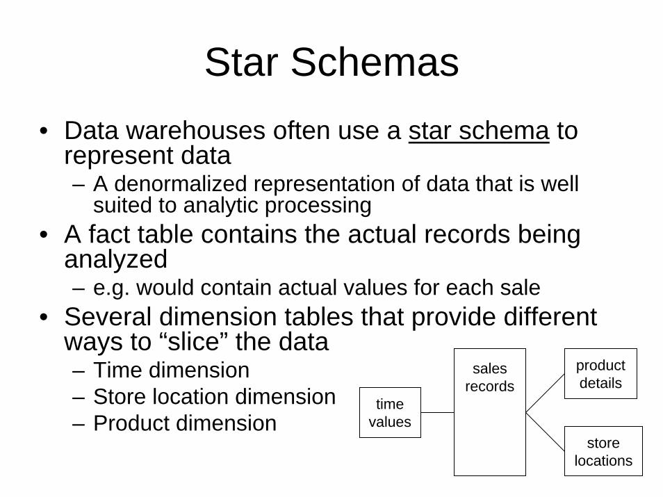
Star Schemas• Data warehouses often use a star schema to
represent data– A denormalized representation of data that is well
suited to analytic processing• A fact table contains the actual records being
analyzed– e.g. would contain actual values for each sale
• Several dimension tables that provide different ways to “slice” the data– Time dimension– Store location dimension– Product dimension
salesrecords
timevalues
storelocations
productdetails
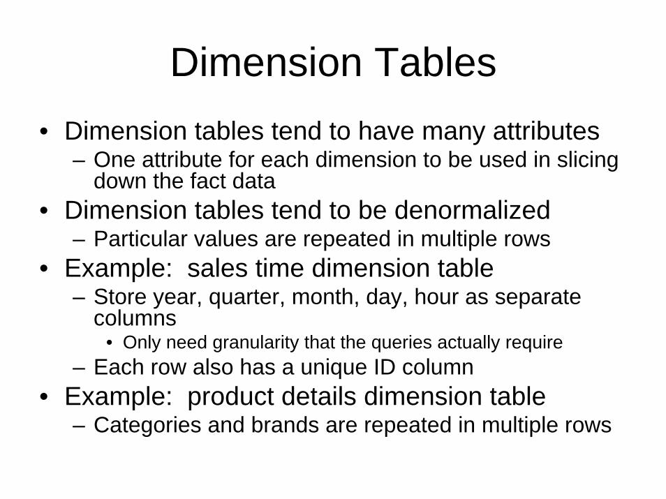
Dimension Tables• Dimension tables tend to have many attributes
– One attribute for each dimension to be used in slicing down the fact data
• Dimension tables tend to be denormalized– Particular values are repeated in multiple rows
• Example: sales time dimension table– Store year, quarter, month, day, hour as separate
columns• Only need granularity that the queries actually require
– Each row also has a unique ID column• Example: product details dimension table
– Categories and brands are repeated in multiple rows

Dimension Tables (2)• Can also normalize dimension tables
– Eliminates redundancy in dimension tables by normalizing them
– Yields a snowflake schema– Increases complexity of query formulation and query
processing– Star schemas usually preferred, unless dimensions
include extensive hierarchy and need normalizing• Dimension tables tend to be small
– …at least, compared to the fact table!– Could still be up to tens of thousands of rows

The Fact Table• Fact table stores aggregated values for the
minimal granularity of each dimension– Time dimension normally drives this granularity
• e.g. “daily totals” or “hourly totals”• Fact tables tend to have fewer columns
– Only contain the actual facts to be processed– Dimensional data is pushed into dimension tables– Each fact refers to associated dimension values using
foreign keys– Combination of foreign keys forms a primary key for
the fact table• Fact table contains the most rows, by far
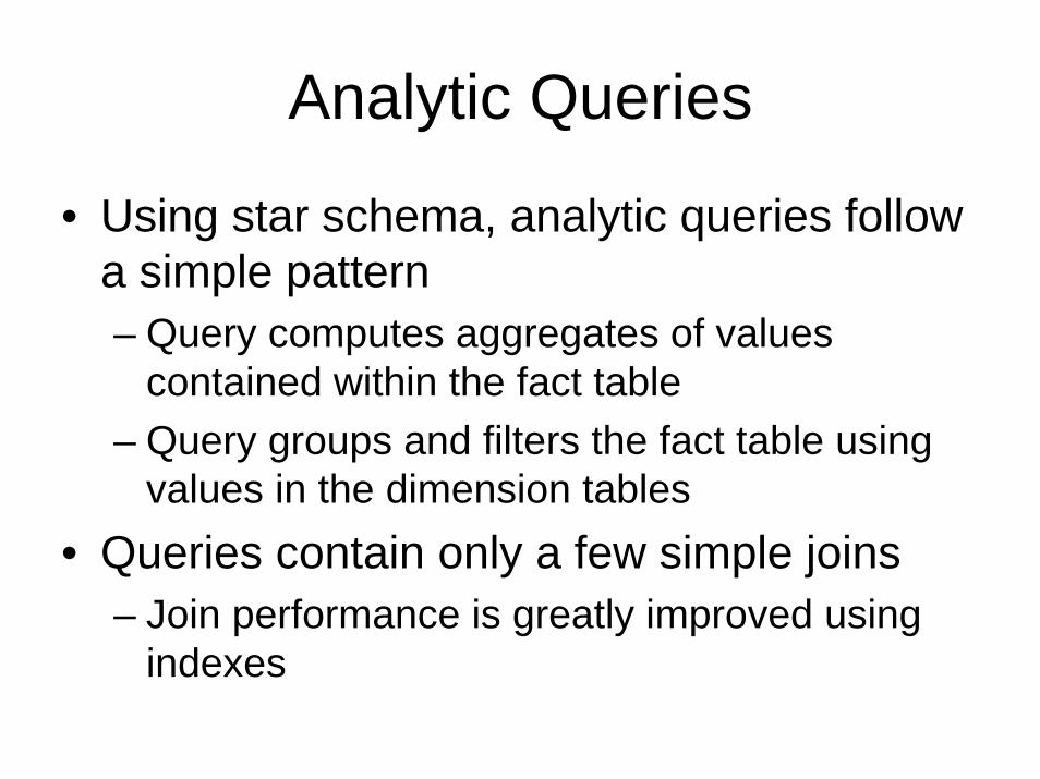
Analytic Queries
• Using star schema, analytic queries follow a simple pattern– Query computes aggregates of values
contained within the fact table– Query groups and filters the fact table using
values in the dimension tables• Queries contain only a few simple joins
– Join performance is greatly improved using indexes

Data Warehouses• Approach is called dimensional analysis• Good example of denormalizing a schema to
improve performance– Using a fully normalized schema will produce
confusing and slow queries• Decompose schema into a fact table and several
dimension tables– Queries become very simple to write, or to generate– Database can execute queries very quickly
• Databases are providing more OLAP features– SQL:1999 provides enhanced grouping syntax– Most vendors have OLAP enhancements as well


![A History and Evaluation of System Rusers.cms.caltech.edu/~donnie/dbcourse/intro0607/papers/SystemR.pdf · Introduction Throughout the ... C.J. Date [27] defined data independence](https://static.documents.pub/doc/80x56/5b16f58b7f8b9a79458b71b8/a-history-and-evaluation-of-system-donniedbcourseintro0607paperssystemrpdf.jpg)


