DataSet - Software - Eigenvector Research,...

DataSet Standard Data Object

for use with MATLAB™

Version 5.0, Released July 11, 2007

Page 2

Eigenvector Research, Inc., Software License Agreement

READ THE TERMS AND CONDITIONS OF THIS LICENSE AGREEMENT CAREFULLY BEFORE OPENING THIS PACKAGE OR USING THIS SOFTWARE. THIS LICENSE AGREEMENT REPRESENTS THE ENTIRE AGREEMENT BETWEEN YOU (THE “LICENSEE” - EITHER AN INDIVIDUAL OR AN ENTITY) AND EIGENVECTOR RESEARCH, INC., (“EVRI”) CONCERNING THE DATASET COMPUTER SOFTWARE CONTAINED HEREIN (“PROGRAM”), AND THE ACCOMPANYING USER DOCUMENTATION. BY OPENING THIS PACKAGE OR USING THE SOFTWARE, YOU ACCEPT THE TERMS OF THIS AGREEMENT.

LICENSE GRANT: All copies of Program and Documentation shall contain all copyright and proprietary notices in the originals. Licensee shall not re-compile, translate, or convert “M-files” contained in the Program for use with any software other than MATLAB®, which is a product of The MathWorks, Inc. 24 Prime Park Way, Natick, MA 01760, without express written consent of EVRI.

LIMITED WARRANTY; LIMITATION OF REMEDIES. Program does not come with a warranty expressed or implied. THE FOREGOING WARRANTY IS IN LIEU OF ALL OTHER WARRANTIES, EXPRESS OR IMPLIED, INCLUDING BUT NOT LIMITED TO THE WARRANTIES OF MERCHANTABILITY AND FITNESS FOR A PARTICULAR PURPOSE. EVRI SHALL NOT BE LIABLE FOR ANY SPECIAL, INCIDENTAL, OR CONSEQUENTIAL DAMAGES, INCLUDING WITHOUT LIMITATION LOST PROFITS. Licensee accepts responsibility for its use of the Program and the results obtained therefrom.

LIMITATION OF REMEDIES AND LIABILITY. IN NO EVENT WILL EVRI BE LIABLE TO YOU FOR ANY DAMAGES, INCLUDING LOST PROFITS, LOST BENEFITS, OR OTHER INCIDENTAL OR CONSEQUENTIAL DAMAGES, RESULTING FROM THE USE OF OR INABILITY TO USE THE PROGRAM OR ANY BREACH OF WARRANTY. EVRI’s LIABILITY TO YOU FOR ACTUAL DAMAGES FOR ANY CAUSE WHATSOEVER, AND REGARDLESS OF THE FORM OF ACTION, WILL BE LIMITED TO THE MONEY PAID FOR THE PROGRAM OBTAINED FROM EVRI THAT CAUSED THE DAMAGES OR THAT IS THE SUBJECT MATTER OF, OR IS DIRECTLY RELATED TO, THE CAUSE OF ACTION. Some states do not allow the exclusion or limitation of incidental or consequential damages, so the above limitation may not apply to you.

GENERAL PROVISIONS. Should any act of Licensee purport to create a claim. lien, or encumbrance on any Program, such claim, lien, or encumbrance shall be void. All provisions regarding indemnification, warranty, liability and limits thereon, and protection of proprietary rights and trade secrets, shall survive termination of this Agreement, as shall all provisions regarding payment of amounts due at the time of termination. Should Licensee install the Programs outside the United States, Licensee shall comply fully with all applicable laws and regulations relating to export of technical data. This Agreement contains the entire understanding of the parties and may be modified only by written instrument signed by both parties.

GOVERNMENT LICENSEES. RESTRICTED RIGHTS LEGEND. Use, duplication, or disclosure by the U.S. Government is subject to restrictions as set forth in subparagraph (c)(1)(ii) of the Rights in Technical Data and Computer Software clause at DFARS 52.227-7013. Licensor is Eigenvector Research, Inc., 830 Wapato Lake Road, Manson, WA 98831, USA.

Page 3

Table of Contents TABLE OF CONTENTS ................................................................................................. 3

INTRODUCTION TO THE STANDARD DATASET OBJECT ................................ 4

1. DATASET INSTALLATION...................................................................................... 5 1.A. INSTALLING THE DATASET OBJECT........................................................................... 5 1.B. INSTALLING DATASET DEMONSTRATIONS ................................................................ 5

2. STANDARD DATASET OBJECT SPECIFICATIONS .......................................... 5 2.A. BASIC DATASET OBJECT FIELD DESCRIPTIONS ......................................................... 6 2.B. INTRODUCTION TO ADVANCED DATASET OBJECT FEATURES ................................... 8 2.C. DETAILED DISCUSSION OF DATASET OBJECT PROPERTIES (FIELDS) ......................... 9

3. DATASET OBJECT METHODS ............................................................................. 17 CAT................................................................................................................................. 18 DELSAMPS....................................................................................................................... 20 DISP ................................................................................................................................ 22 EXPLODE......................................................................................................................... 23 GET ................................................................................................................................. 24 HORZCAT ........................................................................................................................ 27 ISEMPTY.......................................................................................................................... 29 LENGTH........................................................................................................................... 30 NDIMS ............................................................................................................................. 31 NUMEL............................................................................................................................ 32 PERMUTE ........................................................................................................................ 33 REPMAT .......................................................................................................................... 34 SET.................................................................................................................................. 35 SIZE ................................................................................................................................ 38 SORTROWS...................................................................................................................... 39 SUBSASGN....................................................................................................................... 40 SUBSREF ......................................................................................................................... 42 SQUEEZE ......................................................................................................................... 44 TRANSPOSE ..................................................................................................................... 45 UNIQUE ........................................................................................................................... 46 VERTCAT......................................................................................................................... 47

4. EXAMPLE................................................................................................................... 49

5. FUTURE MODIFICATIONS.................................................................................... 51

REFERENCES................................................................................................................ 52

Page 4

Introduction to the Standard DataSet Object

Data sets include far more ancillary information than simple tables of numbers and the DataSet object was designed as a standard container that can hold all of this information. The standard DataSet object is similar to a structure object defined in MATLAB but it is intended to standardize how data is organized and maintained. The purpose of this document is to define standards and conventions for the standard DataSet object developed and maintained by Eigenvector Research, Inc. (EVRI). It is the intention of EVRI that the DataSet be of an open architecture and independent of any toolboxes. For example, the DataSet is used in the PLS_Toolbox written by EVRI, but it does not require any of the PLS_Toolbox functions or scripts. Although the open architecture allows for user modifications, suggestions for modifications and enhancements should be forwarded to EVRI ([email protected]) who will make free updates available at (www.eigenvector.com).

The goals of the DataSet are: 1) Standardize data set storage into a single compact variable. This includes descriptions, ancillary information, and tools that can be used in the development of data analysis tools. 2) Standardize data function input/output. The DataSet offers a compact form for passing data and information. And, 3) allow open and cost free use for MATLAB users.

Page 5

1. DataSet Installation

1.a. Installing the DataSet Object

The DataSet object constructor and methods are contained in the @dataset folder. To be available, the @dataset folder must be a sub-folder of a folder that is on the MATLAB path. For more information see the MATLAB documentation on setting the path and on object oriented programming.

1.b. Installing DataSet Demonstrations

Demonstrations are not installed into the @dataset folder. Instead they must be added to a folder directly on the MATLAB path.

2. Standard DataSet Object Specifications

The design of the DataSet object included outside input from data analysts, users, instrument manufacturers, and software developers. Not all of the suggested properties and methods were included in the present version, however many may be included in future versions. Users are encouraged to make suggestions for future versions. The following considerations were implemented in the present version:

1. DataSet objects contain single blocks i.e. single data arrays. The data arrays can be two-mode (two-way) or multi-mode (N-way). In this document the number of dimensions (i.e. the return value from the NDIMS function in MATLAB) will be referred to as the number of modes (Kiers, 2000). Thus, a two-way data matrix will consist of 2 modes. The first mode corresponds to rows and the second mode to columns (a third mode is often referred to as tubes or slabs).

DataSet objects can also contain cell arrays in the data field (the .type field is ‘batch’). The cell contents can be used for e.g. variable length batch data. It should be noted that this method of data storage does not support all functionality of the standard DataSet object.

2. There can be multiple sample and variable labels, class identifiers, and numerical scales for each mode (e.g. pinot noir, cabernet, … or spectra, process, etc.).

3. Labels, class identifiers, and numerical scales can be given names corresponding to each label set and mode.

4. Each mode can have multiple corresponding mode titles (e.g. wine or measurement). There are as many titles as modes and usually measurement units are included.

5. The DataSet object is open and editable, however suggestions for changes and enhancements should be made to EVRI.

Page 6

6. The DataSet object can be extracted so that all fields become standard MATLAB class objects (e.g. double, or cell) in the workspace.

2.a. Basic DataSet Object Field Descriptions

The following gives a general description of the fields in a DataSet object and is only meant to give an orientation to the different concepts involved in the DataSet object. See Section 4 to learn more about the MATLAB commands used to create a DataSet object.

Consider a table of data which includes the amount of alcohol consumed by five different countries. In addition, we also have a textual class indicating which continent the given country is on and an otherwise unspecified "Sample Group" which indicates another (otherwise unspecified) sub-sampling of the 5 countries.

Country Continent Sample Group Liquor Wine Beer France Europe 1 2.5 63.5 40.1 Italy Europe 1 0.9 58 25.1 UK Europe 2 1.5 12.2 100 U.S.A. North America 2 2 8.9 87.8 Mexico South America 3 0.8 0.2 50.4

Data: The Data field of a DataSet object contains the numerical component of a given data set. In this example, the three columns on the right are the actual numerical data (columns 4 through 6, rows 2 through 6) and would be stored in the data field. In nearly all cases, rows are observations or objects and columns are variables (one observes a variable for a number of objects). Note that although the column "Sample Group" contains numerical data, it is contextual data – that is, data which gives context to the samples – not true numerical data. You can tell it is contextual because we could just as easily replace the numbers with descriptive strings ("Primary", "Secondary", etc) and not influence the interpretation (in fact, using strings, such as was done in the "Continent" column, would be more interpretable and probably preferable!)

Labels: A DataSet object also allows for Label sets to be associated with each mode (rows or columns, in this example). Labels are usually not used by algoirthms and are used only to give contextual information on individual rows or columns. Here, the first column is a set of labels indicating the name of each country. This item would be stored as "Labels" for the rows of the DataSet object. The "Label Name" for this column would be "Countries".

Likewise, the first row (just above the numbers, comprising: "Liquor", "Wine", "Beer") are labels for the columns of the DataSet object and would be stored as Labels for columns. The Label Name for these labels would be "Alcohol Type" (or something similar). Note that you can have any number of Label "sets" for a given mode.

Classes: Classes, like labels, are contextual information for the data and give information on similarities between different rows or columns. Although the second column (titled here as "Continent") could be stored as a second set of row labels, it is more appropriate to use this particular column as a Class set. Classes are very similar to labels with the

Page 7

notable difference that, because classes usually describe how the data can be split into sub-groups, a given string class is often used for more than one sample (note that "Europe" appears for each of the first three countries). Compare this to labels which usually give unique information for a given item. Classes also provide an easy way to select and/or modify the group of rows or columns as a whole.

Another difference between classes and labels is that classes can be referred to using either strings or numerical values. If you assign classes using numerical values, strings will automatically be created to describe the different class groups. See the description of the .class and .classid fields in the next section for more information. For example, in this table, the "Sample Group" column would be most appropriate as a class set for rows and could be assigned as a numerical class.

As with labels, classes can also have a "class name" which is a general descriptor for the class. In this example, it would be appropriate to give a class name of "Continent" for the first class set and "Sample Group" for the second class set. Note that, although it is possible to do, there are no classes given for the columns in this example.

Axisscales: Another type of contextual information which can be stored in a DataSet object is an axis scale. Axisscales are used when samples or variables have a natural order and numerical relationship. Although this example does not contain such ordered data, an example would be when measuring something as a function of time. Each row (observation) would have a time-stamp associated with it. These values would be stored in the axisscale field (note: because the field name does not have a space in it, this document will refer to axis scales without the space, "axisscale").

In addition to axisscale, there is also a DataSet object field named axistype which allows the categorization of the relationship between adjacent items in a given mode. Often used in conjunction with axisscale, axistype specifies whether consecutive items (e.g. columns) should be considered "discrete", unrelated items; "stick" items which are unrelated but have reference to zero in the y-scale; "continuous" items which are generally accepted as individual points on a continuous surface or line; or "none" which indicates no relationship has been established. Some plotting commands will use the axistype information to determine how plots of the given data should be generated.

Include: One of the key features of the DataSet object is the ability to "soft-delete" an item. This is accomplished using the Include field of the DataSet object. The include field simply lists all the items which should be considered when working with the given dataset. In this example, we might want to ignore the non-European countries which we would do by setting the include field of the DataSet object to include only the first three rows (ignore rows 4 and 5, U.S.A. and Mexico)

Title: In addition to the fields which include one entry for each row or column of the table, there is also a generic "title" field which includes a single description for the entire mode. This is often used to describe what the given mode is being used for, such as "Samples" (mode 1, i.e. rows, for the table above).

Page 8

2.b. Introduction to Advanced DataSet Object Features

Indexing into DataSet Objects: Users familiar with MATLAB know that any subset of an n-dimentional matrix can be retrieved from the whole matrix using standard parenthesis and indexing. DataSet objects are handled identically. For example, to obtain a DataSet object comprised of only the 3rd row of a two-way DataSet object, x, the following command would be used:

sub = x(3,:);

The returned variable will be a DataSet object with all the contextual data for the given subset of the original DataSet object.

In addition to this standard indexing, a special indexing is available which makes use of the labels defined for a DataSet. By giving the DataSet name, followed by a period and the label of any row, column, or other n-dimensional item, will return that single item in a DataSet object. For example, given a DataSet which has a column with the label "sensor", the following would extract that column as a new DataSet object:

sub = x.sensor;

The only restrictions to this style of indexing are:

1) If the label contains any spaces or other MATLAB reserved character (e.g. mathematical symbols such as plus or minus), you must enclose the label in parenthesis and single quotes:

sub = x.('sensor number 2');

2) The label may not be the same as any standard DataSet object field or method.

Multiway Data: DataSet objects can contain data structures which are more complex than simple tables. One example mentioned above is Multi-way arrays (data which is most appropriately described using 3 or more dimensions). These cases are direct extensions of the two-way example given above. Each mode has its own labels, classes, and axisscales.

Image Data: Another example of complex data which can be stored in a DataSet object is Image data. By setting the type field of a DataSet object to be "image", one can store image data where each pixel (or voxel, in the case of volumetric 3D images) is an observation. Such DataSet objects store the data as "unfolded" (where all the spatial positions are stored in a single mode) and, thus, require information on how to arrange the observations back into the spatial image. This is accomplished with the imagemode and imagesize fields.

Batch Data: Finally, there is intermediate support for batch data which is described as a series of two-way tables (or higher dimensional, if desired) of different lengths. In this document, the features available for this type of data are referred to as type=batch

Page 9

DataSet objects.

2.c. Detailed Discussion of DataSet Object Properties (Fields)

The following is a list of the DataSet object properties (fields). The values in all fields can be assigned or retrieved using direct assignments (See SUBSASGN and SUBSREF in Section 3) or through the SET and GET methods (also described in Section 3) although direct assignments are the preferred of those two methods. For a walk-through example of how to build a DataSet object, see Section 4.

.name char array (row vector)

This is usually the original variable name but can be set by the user. For example: h = dataset(randn(5)); h.name = ‘mydata’; h.name ans = mydata

where ans is a 1x6 character array.

.type row char array with one of the following values

‘data’, ‘image’, and ‘batch’. See field ‘.data’ for more information on these data types.

When .type = 'image', three additional fields are available in the DataSet: .imagemode, .imagesize, .imagedata, and .imageinclude. Each of these fields is described below.

.author char array (row vector)

Used to assign authorship to a DataSet. h.author = ‘Joan Smith / Big Name Pharma’;

.date double array (1x6)

Six-element date/time stamp [year, month, day, hour, minute, second] indicating when the DataSet was created.

.moddate double array (1x6)

Six-element date/time stamp indicating when the DataSet was last modified.

.data

Field holding the numerical data of the DataSet. Can take one of two forms:

Page 10

1) Fixed-size array (i.e. the data matrix is N1xN2x…xNM) of class: double, single, logical, [u]int8, [u]int16, or [u]int32.

When the data are contained in a standard fixed-size array (field .type = ‘data’ or ‘image’) then M is the number of modes, indices are nm = 1, 2, …, Nm, and m = 1, 2, …, M. This notation follows, but is slightly more general than, the notation proposed by Kiers(2000). For example,

MNA where M=2 is N1xN2.

With multi-block analyses, the first mode (m=1) of the .data array corresponds to the common dimension between blocks (e.g. samples). Any function that changes this convention requires an optional control for sample/object mode.

For example, the following forms a three-slab multiway DataSet: mwa(:,:,1) = randn(5); mwa(:,:,2) = magic(5); mwa(:,:,3) = sin([1:5]’)*cos(1:5); mydatb = dataset(mwa); size(mydatb.data,3) ans = 3

For more information on type 'image' DataSet objects, see the .imagemode field below.

2) cell array (Length I with i = 1, 2, …, I. Each cell contains a double array 1,i mN xNA

with m = 2, 3, …, M. The size of mode 1 (N1,i) for each array can vary from cell to cell. All other modes must be of equal size from cell to cell.)

This data construct allows for matrices that are all the same size except for in the first mode which can be of variable length. This data can not be stored in a multiway array and instead are stored in a cell array (field .type = ‘batch’). This results in differences between double array data that are reflected in SET, GET, and the field .axisscale.

.imagemode double scalar {1x1}

.imagesize double vector {1xMimg}

.imagedata double array

These three fields are only available for type 'image' DataSet objects. In image DataSet objects, the .data field contains "unfolded" image data. Image data is usually contained in a 2nd or higher-order matrix in which several modes are used to describe a spatial relationship between pieces of information. For example, many standard JPEG images are three-way images of size M x N x 3. The first two dimensions are the spatial dimensions in that the actual image is M pixels high by N pixels wide. The third dimension is the wavelength dimension and, in this case, contains 3 slabs – one

Page 11

for each of the Red, Green, Blue image components.

Working with such image data in DataSet objects is made easier by unfolding such multi-way images so that all the spatial modes are stacked on top of each other in a single mode. Unfolding is done so that all the spatial information is contained in a single mode and can be handled together – often so that each pixel can be analyzed as an individual sample (or even sometimes as variables). Individual pixels in an unfolded image are independent and can be individually included and excluded (see .include field) or assigned particular classes (see .class field), for example. In the case of the JPEG mentioned above, the unfolded image would be stored as an (MN) x 3 matrix where the first mode was M times N elements (i.e. pixels) in size.

The .imagemode field contains a scalar value indicating which mode of the .data field contains the spatial information. In the JPEG example, .imagemode would be 1 (one). Similarly the .imagesize field contains a vector describing the original size of the spatial mode before unfolding. The JPEG example would contain the two-element vector: [M N] Note: that .imagesize contains only the size of the image mode, not the entire data matrix. Note that the product of the .imagesize field must be equal to the size of the .imagemode mode of the .data field. That is, the number of pixels contained in the spatial mode of the data must be appropriate that it can be reshaped into a matrix of size .imagesize.

The .imagedata field is a special read-only field which returns the contents of the .data field refolded back into the original image-sized matrix. In the JPEG example, the .data field would return a matrix of size (MN) x 3 (the unfolded image) but the .imagedata field would return the original M x N x 3 matrix. Any changes you make to the contents of the .data field will automatically be reflected in the contents returned by .imagedata. .imagedata, however, can not be written to.

To create a type 'image' DataSet object:

(a) Unfold the spatial mode of the original data (the following example is for three way data but is easily extended to multi-way images):

sz = size(x); x = reshape(x, sz(1)*sz(2), sz(3));

(b) Create the standard DataSet object (type='data') from the unfolded data: imgdso = dataset(x);

(c) Change the DataSet object type to 'image': imgdso.type = 'image';

(d) And store the original image size in the DataSet

Page 12

imgdso.imagemode = 1; imgdso.imagesize = sz(1:2);

Note that although this example shows the image being unfolded into the first mode, there is no requirement that the first mode be the pixel mode. The first mode is, however, the most consistent with the concept that individual pixels are often considered separate samples. Use the permute function on x prior to creating the DataSet (before step (b) above) to move the spatial mode to a different dimension.

.label cell array {MxSlbls}

Each column of the cell contains char arrays of labels for each mode of ‘.data’ (the cell entries may be empty.) The first row corresponds to labels for the first mode of ‘.data’ and contains char arrays with N1 rows. Subsequent rows of the cell contain labels for corresponding modes of ‘.data’ each of which are char arrays with Nm

rows. Additional columns contain alternate sets of labels for all modes.

Assignments to individual cell elements may be a character array or a cell array. Labels are always converted to character arrays when retrieved.

For example, suppose there is a DataSet object x. Its labels for the mth mode are contained in x.label{m,1}. If there is a second set of labels for this mode, they are contained in x.label{m, 2}. The following sets the second set of labels for the first mode of DataSet x assuming size(x.data,1) = 3

x.label{1,2} = {‘firstlabel’,’secondlabel’,’thirdlabel’};

An individual label in any set can be changed by adding an additional index using "curly braces" (the ones used for cell indexing) and the string which should be used. For example, changing the second row's label (in the second set) would be accomplished using:

x.label{1,2}{2} = ’New second label’;

.labelname cell array {MxSlbls}

Each column of the cell is associated with the corresponding column of ‘.label’ and contains string descriptions (each a row char array) of the corresponding labels for each mode of ‘.data’ (e.g. ‘Mode 1 Lbls’, ‘Mode 2 Lbls’, …). Additional columns contain alternate sets of label names.

For example, the label name associated with the first set of labels for mode m is contained in x.labelname{m,1}.

.axisscale

1) cell array {MxSscale} (when ‘.data’ is a fixed-size array)

Page 13

When ‘.data’ is a fixed-size array (other than cell), each column of the cell contains a set of axis scales (a total of Mx1 vectors, each Nmx1 of class double) for each mode of ‘.data’ (e.g. a time axis, or sample number). Rows of the cell correspond to modes of ‘.data’ (e.g. a wavelength axis, or variable number). Additional columns of ‘.axisscale’ contain alternate sets of axis scales for all modes.

For example, suppose there is a DataSet object x. Its axis scale for the mth mode are contained in x.axisscale{m,1}. If there is a second set of axis scales they are contained in x.axisscale{m,2}. The following sets the first set of axisscales for the third mode of DataSet x assuming size(x.data,3) = 10

x.axisscale{3,1} = 1:10;

2) cell array {MxSscale} (when ‘.data’ is a cell array)

When ‘.data’ is class cell, the contents of ‘.axisscale’ are similar to those described above, except for mode 1 (i.e. first row of the ‘.axisscale’ cell). In this case, the contents of the first row contain cell arrays (in contrast to vectors of class double) whose contents are axis scales (Nn1x1 vectors). Each axis scale corresponds to the first mode of each cell of ‘.data’ (e.g. a time axis, or sample number). This allows for variable axis scales when the data matrices are of variable length in the first mode. Subsequent rows of the cell contain scales (Nmx1 vectors) for corresponding modes of ‘.data’ (e.g. a wavelength axis, or variable number) just as when ‘.data’ is a fixed-size array.

.axisscalename cell array {MxSscale}

Each column of the cell is associated with the corresponding column of ‘.axisscale’ and contains string descriptions (each a row char array) of the corresponding axis scale for each mode of ‘.data’ (e.g. ‘Mode 1 Axis’, ‘Mode 2 Axis’, …). Multiple columns contain alternate sets of axis scale names.

For example, the axis scale name associated with the first set axis scale for mode m is contained in x.axisscalename{m,1}.

.axistype cell array {MxSscale}

The 'axistype' field is informational only and does not effect other properties of the DataSet object. The axistype field identifies the relationship between adjacent elements in the corresponding axisscale (same mode and set). Axistype identifies this relationship using one of the following keywords:

none : {default} a relationship between values is not known. Software may default to whatever display and calculation mode desired.

discrete : Individual items (e.g. columns) are discrete of each other and should not be interpolated between in plots or other numerical operations. Show as individual points.

Page 14

stick : Individual items (e.g. columns) are discrete of each other and should not be interpolated between in plots or other numerical operations, however, each item has a connection to a value of zero at the given axisscale position (e.g. sticks down to the zero line on the y-axis)

continuous : Individual items (e.g. columns) are considered points on a continuous axis and may be interpolated between in plots and other numerical operations.

When concatenating two datasets with different axistypes for the concatenation mode, the least-presumptive axistype in this list will be used. That is, "none" will be selected over "discrete" which will be selected over "stick" which would be selected over "continuous".

Although some software makes use of this field to help customize plots and numerical operations, it is not required operation.

.title cell array {MxStitle}

Each column of the cell contains a set of mode titles (each a char array) for each mode of ‘.data’. Rows of the cell correspond to modes of ‘.data’ and additional columns of ‘.title’ contain alternate sets of mode titles for all modes.

For example, suppose there is a DataSet object x. Its mode title for the mth mode is contained in x.title{m,1}. If there is a second set of mode titles they are contained in x.title{m,2}.

.titlename cell array {MxStitle}

Each column of the cell is associated with the corresponding column of ‘.title’ and contains string descriptions (each a row char array) of the corresponding mode titles for each mode of ‘.data’ (e.g. ‘Mode 1 Title’, ‘Mode 2 Title’, …). Additional columns contain alternate sets of mode title names.

For example, the mode title name associated with the first set mode title for mode m is contained in x.titlename{m,1}.

.class cell array {MxSclass}

Each column of the cell contains a set of class identifiers (each an Nmx1 vector) for each mode of ‘.data’. Rows of the cell correspond to modes of ‘.data’ and additional columns contain alternate sets of class identifiers for all modes.

For example, suppose there is a DataSet object x. Its class identifier for the mth mode is contained in x.class{m,1}. If there is a second set of class identifiers they are contained in x.class{m,2}. See example for axisscale field.

Assignments into class can be either numeric (assigning an appropriate-length vector of numbers) or string (using an appropriate-length cell array of strings). However,

Page 15

retrieving values from the .class field will always return numerical values. See the classid field to retrieve classes as strings instead of numerical values and the classlookup field to retrieve the table used to translate numerical classes to string values.

.classid cell array {MxSclass}

This field is a pseudonym for the class field and is indexed exactly the same except that when retrieving values from this field, the returned value is a cell array of strings where each string represents the class of the object (row, column, etc). Assignments to this field can also be either class strings or numerical class values. See also the classlookup field to retrieve the table used to translate numerical classes to string values.

.classlookup cell array {MxSclass}

The classlookup field is sized the same as the class field but each entry contains a lookup table, structured as a k by 2 cell array. This lookup table contains the numerical class values in the first column and the corresponding class name in the second column. A shortcut to look up a class number or class string in this table is provided by adding the indexing command find() onto the end of the classlookup extraction command. Given a DataSet object, x, with a set of row classes:

x.classlookup{1,1}.find(val)

returns the string associated with the numerical value "val". Likewise:

x.classlookup{1,1}.find('string')

returns the numerical class value associated with the class description string 'string'.

Assignment into the classlookup field is specially controlled. Individual entries can not be directly edited but, instead, must be changed using the indexing: assignstr or assignval. These commands are given after the .classlookup{mode,set} indexing and are followed by an assignment which gives the new values. For example, given a DataSet object, x, the following notation is used to change the string associated with a given class number:

x.classlookup{1,1}.assignstr = {3 'new string'};

The above would change the string associated with class 3 (of mode 1, set 1) to be 'new string'. Similarly:

x.classlookup{1,1}.assignval = {18 'current string'};

would change the class number associated with the class 'current string' to be 18.

If the entire lookup table is replaced by direct assignment, any class number which

Page 16

appears in the class field but does not appear in the new lookup table will be automatically changed to class 0 (zero) in the class field. Thus, replacing the lookup table can be used to effectively delete a class from the class field.

.classname cell array {MxSclass}

Each column of the cell is associated with the corresponding column of ‘.class’ and contains string descriptions (each a row char array) of the corresponding class identifiers for each mode of ‘.data’ (e.g. ‘Mode 1 Classes’, ‘Mode 2 Classes’, …). Additional columns contain alternate sets of class identifier names.

For example, the class name associated with the first set class identifiers for mode m is contained in x.classname{m,1}.

.include cell array {Mx1} with vector contents

Each row of ‘.include’ contains a vector of indices indicating which samples or variables to use in an analysis. When first constructed the contents of each cell in ‘.include’ is [1:Nm]. The ‘.include’ field allows for sample or variable exclusion (e.g. soft delete) of ‘.data’ rows or columns without actually removing or modifying the raw data in the data set. Note: In earlier versions of the DataSet object this field was named ‘.includ’. Although that field name will be translated into ‘.include’, use of the full field name is recommended.

.description char array containing a description of the data set.

.history running history of commands that have modified the DataSet contents.

.userdata can contain any class and is a container for additional user data.

Note that when DataSet objects are concatenated this can be turned into a cell array containing user data from each concatenated object in the cell containers.

Page 17

3. DataSet Object Methods

In addition to the specific methods listed below, a number of standard MATLAB functions are overloaded for DataSet objects but otherwise work as documented for standard data types. The following methods operate on the underlying data field of a DataSet object only and have no effect on any other fields:

minus (-) plus (+) times (.*) rdivide (./) ldivide (.\) double single

To get help on any DataSet object method, use the command: help dataset/method where method is the name of the method for which you want help. % SORTROWS UNQIUE

Page 18

cat

Purpose

Generic concatenation of DataSet objects.

Synopsis

z = cat(dim,a, b, c, ... );

Description

Generic concatenation implies combination of DataSet objects along some specified dimension, dim. Any number of DataSet objects can be concatenated. When dim is 1 or 2, this command is equivalent to [a; b; …] or [a b …], respectively (see dataset/vertcat and dataset/horzcat).

For this operation to be defined the following must be true:

1) All inputs must be valid DataSet objects or convertible to a DataSet object.

2) The DataSet '.type' fields must all be the same.

3) Concatenation is along the specified dimension (dim). All other dimension sizes must match.

This is similar to matrix concatenation, but each field is treated differently. In structure notation this is:

z.name = name fields from all DataSet objects are concatenated. z.type = a.type; z.author = author fields from all DataSet objects are concatenated. z.date = date of concatenation z.moddate = date of concatenation z.data = cat(dim,a.data,b.data,c.data); z.label = mode dim label sets are concatenated, and new label sets are

created for all other modes z.axisscale = mode dim axisscale sets are made empty, and new axisscale

sets are created for all other modes z.title = new label sets are created z.class = mode dim class sets are made empty, and new class sets are

created for all other modes z.description = concatenates all descriptions z.userdata = if more than one input has userdata it is filled into a cell

array, if only one input has userdata it is returned, else it is empty

Page 19

Example: The following concatenates two DataSet objects, a and b, along the third dimension (slabs):

z = cat(3,a,b); %join a and b in the third dimension

See Also

dataset, datasetdemo, dataset/horzcat, dataset/vertcat

Page 20

delsamps

Purpose

Deletes or excludes the specified samples, rows, or other dimension from a DataSet object.

Synopsis

eddata = delsamps(data,inds,vdim,flag)

Description

DELSAMPS modifies the include field of a DataSet to mark rows or columns to be "excluded" keeping the data in the DataSet (i.e. soft delete). It can also be used to permanently remove rows or columns from a DataSet object (i.e. hard delete).

Inputs are the original DataSet object, data, and the indices to mark, inds. Optional input vdim is the mode/dimension to mark

1=rows {default}, and

2=columns, etc.

Optional input (flag) indicates to mark/soft delete when set to 1 {default}, hard delete when set to 2, or hard "keep" when set to 3. The output is the edited DataSet object (eddata).

Examples:

The first example returns a DataSet object with the first two rows (samples) excluded (soft delete), the second hard-deletes the first two columns:

a = delsamps(a,[1 2]); %soft delete rows 1 and 2

a = delsamps(a,[1 2],2,2); %hard delete columns 1 and 2

When flag = 3, the function of inds is inverted and indicates the indices to keep (all others are deleted). The order the indices appear in inds specifies the new order of the rows/columns/etc. in the result. Thus, the delsamps command

eddata = delsamps(data,inds,2,3);

is equivalent to performing the operation (see dataset/subsref):

eddata = data(:,inds);

Page 21

See Also

datasetdemo, dataset/subsref

Page 22

disp

Purpose

Display summary of DataSet object contents.

Synopsis

disp(x)

Description

Displays a summary of the given DataSet object's contents in the console window.

See Also

dataset

Page 23

explode

Purpose

Extract all variables from a DataSet object.

Synopsis

explode(x,txt)

Description

EXPLODE writes the fields of a DataSet input x to variables in the workspace with the same variable names as the field names. The optional string input txt appends a string txt to the variable outputs.

Example:

explode(h,'01')

See also

dataset/get, dataset/subsref

Page 24

get

Purpose

Get field/property values from a DataSet object.

Synopsis

value = get(x,'field',vdim);

Description

dataset/get is a depreciated function. See dataset/subsref for the preferred method of extracting values from a DataSet object.

The I/O for GET depends on whether the data are of class double or cell. The more common usage is when the data are of class double and this is discussed under subheading 1. In this case the data can be contained in a double array of 2 or higher modes/dimensions. Differences for data of class cell are discussed under subheading 2.

1) The following is used when the data field is a fixed-size array (.type = ‘data’ or ‘image’)

value = get(x,'field');

For DataSet x this returns the value (value) of the property 'field'. This syntax is used for the following fields:

name: value is a char vector. author: value is a char vector. date: value is a 6 element vector (see CLOCK). moddate: value is a 6 element vector (last modified date). type: value is either 'data' or 'image'. data: value is a double array. description: value is a char array. userdata: user defined. description: value is a char array. history: cell array of char (e.g. char(get(h,’history’))) datasetversion: dataset object version.

Example:

get(x,’data(:,1)’) extracts the first column of the double array.

value = get(x,'field',vdim);

Page 25

This syntax is used with the following fields:

include: value is row vector of indices for mode vdim.

value = get(x,'field',vdim,vset);

Returns the value value for the property 'field' for the specified dimension/mode vdim and optional set vset {default: vset=1}. E.g. vset is used when multiple sets of labels are present in x. This syntax is used for the following fields:

label: value is a char array with size(x.data,vdim) rows. labelname: value is a char row vector. axisscale: value is a row vector with size(x.data,vdim) real

elements. axisscalename: value is a char row vector. title: value is a char row vector. titlename: value is a char row vector. class: value is a row vector with size(x.data,vdim) integer

elements. classname: value is a char row vector.

2) For cases when the data set consists of multiple matrices of variable length (e.g. each data matrix is N1,ixNm, m = 2, …, M; and N1,i¹N1,j for i¹j) the field ‘.data’ can contain a cell array and the field ‘.type’ is ‘batch’. The following are specific to GET when the data field is of class cell (.type = ‘batch’). For fields not listed below use the I/O syntax listed under subheading 1.

value = get(x,'field');

Returns the value value of the property 'field'. This syntax is used for the following fields: type: value is ‘batch’. data: value is a cell array (extracts entire data set).

Example: get(x,’data{3}(:,1)’) %extracts the first column of the third cell get(x,’data{2}’) %extracts the entire contents of the second cell.

value = get(x,'field',vdim,vset);

Returns the value value of the property 'field' for the specified dimension/mode vdim and optional set vset {default: vset=1}. E.g. vset is used when multiple sets of labels are present in x. This syntax is used for the following fields:

axisscale: value is a row vector with size(x.data,vdim) real elements. For all but the first mode the I/O syntax is identical to

Page 26

that for data of class double discussed under subheading 1. For mode 1 vdim is either scalar value 1 (i.e. vdim=1), or a two element vector with vdim(1)=1 and vdim(2)=i where i = 1, …, N1.

Example:

get(x,’axisscale’,1,2) extracts the entire cell array of axis scales for mode 1 from the second set

get(x,’axisscale’,[1 3]) extracts the axis scales for mode 1 of the 3rd

cell from the first set

See also:

datasetdemo, dataset/set, dataset/subsref, dataset/explode

Page 27

horzcat

Purpose

Horizontal concatenation of DataSet objects.

Synopsis

z = [a, b, c, ... ];

Description

[a b] is the horizontal concatenation of DataSet objects a and b. Any number of DataSet objects can be concatenated within the brackets. For this operation to be defined the following must be true:



3) Concatenation is along the second dimension. The first and, for multiway, remaining dimension sizes must match.


z.name = name fields from all DataSet objects are concatenated. z.type = a.type; z.author = author fields from all DataSet objects are concatenated. z.date = date of concatenation z.moddate = date of concatenation z.data = [a.data b.data c.data ...]; z.label = mode 2 label sets are concatenated, and new label sets are

created for all other modes z.axisscale = mode 2 axisscale sets are made empty, and new axisscale

sets are created for all other modes z.title = new label sets are created z.class = mode 2 class sets are made empty, and new class sets are



Page 28

See Also

dataset, datasetdemo, dataset/cat, dataset/vertcat

Page 29

isempty

Purpose

Returns Boolean true if the DataSet object data field is empty.

Synopsis

e = isempty(x);

Description

Returns a value of true (logical(1)) if the given DataSet object has an empty data field, otherwise, a value of false (logical(0)) is returned.

See Also

dataset/end, dataset/length, dataset/size, dataset/subsref, dataset/ndims

Page 30

length

Purpose

Returns the length of the data field in a DataSet object.

Synopsis

l = length(x);

Description

Returns the length of a DataSet .data field. It is equivalent to MAX(SIZE(X)) for non-empty arrays and 0 for empty ones. See built-in Matlab function LENGTH for more information.

See Also

dataset/end, dataset/isempty, dataset/size, dataset/subsref, dataset/ndims

Page 31

ndims

Purpose

Returns the number of dimensions of the data field in a DataSet object.

Synopsis

D = ndims(x);

Description

Returns the number of dimensions (i.e. modes) of a DataSet .data field.

Example: The following returns the number of dimensions in the .data field of a three-way DataSet object, a:

>>ndims(a) ans = 3

See Also

dataset/size

Page 32

numel

Purpose

Returns a value of 1 for any dataset object.

Synopsis

D = numel(x);

Description

WARNING! This overloaded function always returns a value of 1 (one) for any DataSet object, regardless of the number of elements in the data field! This odd behavior is required by MATLAB for any user-defined object.

To get the number of elements stored in the data field of a given DataSet object, use:

numel(x.data)

See Also

dataset/size

Page 33

permute

Purpose

Permute array dimensions of a DataSet object.

Synopsis

x = permute(x,order);

Description

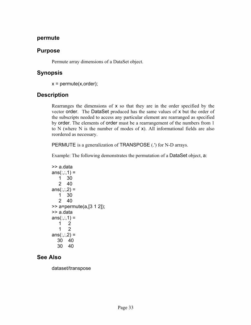
Rearranges the dimensions of x so that they are in the order specified by the vector order. The DataSet produced has the same values of x but the order of the subscripts needed to access any particular element are rearranged as specified by order. The elements of order must be a rearrangement of the numbers from 1 to N (where N is the number of modes of x). All informational fields are also reordered as necessary.

PERMUTE is a generalization of TRANSPOSE (.') for N-D arrays.

Example: The following demonstrates the permutation of a DataSet object, a: >> a.data ans(:,:,1) = 1 30 2 40 ans(:,:,2) = 1 30 2 40 >> a=permute(a,[3 1 2]); >> a.data ans(:,:,1) = 1 2 1 2 ans(:,:,2) = 30 40 30 40

See Also

dataset/transpose

Page 34

repmat

Purpose

Replicate and tile a DataSet object.

Synopsis

B = repmat(A,M,N)

B = REPMAT(A,[M N])

B = REPMAT(A,[M N P ...])

Description

Overload of the Matlab command REPMAT for use with DataSet objects.

Returns the given DataSet object, A, concatenated M times vertically (rows) and N times horizontally (columns). This function can also be used to form n-dimensional matrices by passing a vector of length >2 as the second input to REPMAT.

See the Matlab REPMAT command for more details on the operation of this function

See Also

dataset/cat

Page 35

set

Purpose

Set field/property values for a DataSet object.

Synopsis

set(x,'field',value,vdim,vset)

Description

dataset/set is a depreciated function. See dataset/subsasgn for the preferred method of assigning values to a DataSet object.

The I/O for SET depends on whether the data are of class double or cell. The more common usage is when the data are of class double and this is discussed under subheading 1. In this case the data can be contained in a double array of 2 or higher modes/dimensions. Differences for data of class cell are discussed under subheading 2.

1) The following is used when the data field is of class double (.type = ‘data’ or ‘image’).

set(x) displays all field names and possible values for the input x which is a DataSet.

set(x,'field') displays the possible values for input 'field'.

set(x,'field',value) sets the field for a DataSet object to value.

This syntax is used for the following fields: name: char vector or cell of size 1 with char contents. author: char vector or cell of size 1 with char contents. date: 6 element vector (see CLOCK). type: field '.data' must not be empty to set '.type', can have

value 'data' or 'image'. data: double array. description: char array or cell with char contents. userdata: filled with user defined data.

set(x,'field',value,vdim)

This syntax is used for the following fields:

include: row vector of max length size(x.data,vdim) e.g.

Page 36

1:size(x.data,vdim).


sets the field for a DataSet object to value for the specified dimension vdim and optional set vset {default: vset=1}, e.g. the vset input allows for multiple sets of labels to be used. The field '.data' must not be empty to set the values. This syntax is used for the following fields:

label: character or cell array with size(x.data,vdim) rows

containing labels for the vdim dimension/mode. labelname: row vector of class char or 1 element cell containing a

name for the label set. axisscale: vector of class double (real elements) with

size(x.data,vdim) elements. Each contains an axis scale to plot against for the vdim mode (e.g. x.axisscale{2,1} is a numerical scale for columns, and x.axisscale{1,1} is a numerical scale for rows).

axisscalename: row vector of class char or 1 element cell containing a name for the axis scale.

title: row vector of class char or 1 element cell containing a title for the vdim dimension/mode.

titlename: row vector of class char or 1 element cell containing a name for the title.

class: vector of class double (integer elements) and size(x.data,vdim) elements. Each element is a class identifier that can be used in plotting, classification, or cross-validation.

classname: row vector of class char or 1 element cell containing a name for the class set.

2) For cases when the data set consists of multiple matrices of variable length (e.g. each data matrix is N1,ixNm, m = 2, …, M; and N1,i¹N1,j for i¹j) the field ‘.data’ can contain a cell array and the field ‘.type’ is ‘batch’.

The following are specific to SET when the data field is of class cell (.type = ‘batch’). For fields not listed below use the I/O syntax listed under subheading 1.

set(x,'field',value)

sets the property/field for a DataSet object to value. This syntax is used for the following fields:

type: value ‘batch' set automatically when field is class cell data: value is a cell array (extracts entire data set).

Page 37

Example:

g = dataset; %constructs a DataSet object

set(g,’data’,y) %where y is a N1 x 1 cell

SET will check all the sizes of the contents of y to ensure that only the size of mode 1 varies from cell to cell and will also set the ‘.type’ field to ‘batch’.


Set the field for a DataSet object to value for the specified dimension vdim and optional set vset {default: vset=1}, e.g. the vset input allows for multiple sets of labels to be used. The field '.data' must not be empty to set the values. This syntax is used for the following fields:

axisscale: value is a row vector with size(x.data,vdim) real elements.

For all but the first mode the I/O syntax is identical to that for data of class double discussed under subheading 1. For mode 1 vdim is either scalar value 1 (i.e. vdim=1), or a 2 element vector with vdim(1)=1 and vdim(2)=i where i = 1, …, N1. When vdim=1 then value is a cell array of length N1 and the contents of cell i is a vector of length N1,i. When vdim is a 2 element vector and vdim(2)=i then value is a vector of length N1,i.

Example:

set(g,’axisscale’,y2,1) %where y2 is a N1x1 cell array and the contents of each cell y2{i} (i=1, …, N1) is a vector of length N1,I (i.e. size(get(g,’data{i}’),1)) sets the mode 1 axis scale for all data arrays in ‘.data’.

set(x,’axisscale’,[1:N13],[1 3]) %where N13 = size(get(g,’data{3}’),1) sets the mode 1 axis scale for the 3rd data array (i.e. contents of data{3}).

set(x,’axisscale’,[1:N12],[1 2],2]) %where N12 = size(get(g,’data{2}’),1) sets the mode 1 axis scale for the 2nd data array (i.e. contents of data{2}) for the second set.

See also:

dataset/get, dataset/subsasgn, dataset/subsref

Page 38

size

Purpose

Returns the size of the data field in a DataSet object.

Synopsis

D = size(x,dim);

[M,N,…] = size(x);

Description

Returns the size of a DataSet .data field for the specified dimension dim. If dimension is not specified, sizes for all non-singleton dimensions are returned, either as multiple outputs, M, N, etc, or a single vector.

Example: The following returns the number of columns in the .data field of a DataSet object, a:

cols = size(a,2);

See Also

dataset/end, dataset/length, dataset/subsref, dataset/ndims

Page 39

sortrows

Purpose

Returns the given DataSet object with the first mode (rows) sorted.

Synopsis

D = sortrows(x);

D = sortrows(x,column);

Description

Overload of the standard sortrows command. This method operates exactly as described for standard matrices (see standard sortrows documentation) except that the entire DataSet object is sorted, including the labels, classes, axisscales, etc.

See Also

dataset/unique

Page 40

subsasgn

Purpose

Assign for DataSet objects using Structure and index notation.

Synopsis

x.field{vdim,vset} = value;

Description

x.field = value;

sets the field for a DataSet object to value. This syntax is used for the following fields:

name: char vector or cell of size 1 with char contents. author: char vector or cell of size 1 with char contents. date: 6 element vector (see CLOCK). type: field '.data' must not be empty to set '.type', can have

value 'data' or 'image'. See documentation for type 'batch'.

data: double, single, logical, int or uint array, or cell array (type 'batch' see documentation).

imagemode: scalar double. imagesize: variable-length vector of double. description: char array or cell with char contents. userdata: filled with user defined data.

x.field{vdim} = value;

This syntax is used for the following fields:

include: row vector of maximum length size(x.data,vdim) e.g. 1:size(x.data,vdim).

x.field{vdim,vset} = value;

sets the field for a DataSet object to value for the specified dimension vdim and optional set vset {default: vset=1}, e.g. the vset input allows for multiple sets of labels to be used. The field '.data' must not be empty to set the values. This syntax is used for the following fields:

label: character or cell array with size(x.data,vdim) rows

containing labels for the vdim dimension/mode.

Page 41

labelname: row vector of class char or 1 element cell containing a name for the label set.

axisscale: vector of class double (real elements) with size(x.data,vdim) elements. Each contains an axis scale to plot against for the vdim dimension/mode (e.g. x.axisscale{2,1} is a numerical scale for columns, and x.axisscale{1,1} is a numerical scale for rows). See documentation for type 'batch'.

axisscalename: row vector of class char or 1 element cell containing a name for the axis scale.

title: row vector of class char or 1 element cell containing a title for the vdim dimension/mode.

titlename: row vector of class char or 1 element cell containing a name for the title.

class: vector of class double (integer elements) and size(x.data,vdim) elements. Each element is a class identifier that can be used in plotting, classification, or cross-validation.

classname: row vector of class char or 1 element cell containing a name for the class set.

Examples:

mydataset.author = 'James Joyce';

mydataset.axisscale{2} = [1:.5:25]; %2nd dim axis scale

mydataset.title{1,2} = 'Second title for first dim';

See also:

dataset/get, dataset/set, dataset/subsref

Page 42

subsref

Purpose

Subindex for DataSet objects using Structure and index notation.

Synopsis

value = x.field{vdim,vset}

Description

General overload for the subsref method. This method handles all generic indexing into a DataSet object. Below is a summary of the indexing it enables.

value = x.field;

returns the value (value) of the DataSet object field field. This syntax is used for the following fields:

name: value is a char vector. author: value is a char vector. date: value is a 6 element vector (see CLOCK). moddate: value is a 6 element vector (last modified date). type: value is either 'data' or 'image'. data: value is a double,single, or [u]int8/16/32 array. imagemode: value is a scalar double. imagesize: value is a variable-length vector of double. label: value is the cell of all labels. labelname: value is the cell of all label names. axisscale: value is the cell of all axis scales. axisscalename: value is the cell of all axis scale names. title: value is the cell of all mode titles. titlename: value is the cell of all mode title names. class: value is the cell of all class identifiers. classname: value is the cell of all class identifier names. include: value is a cell with vectors for all included indices

for all modes. userdata: user defined. description: value is a char array. history: cell array of char (e.g. char(x.history)) datasetversion: DataSet object version.

value = x.field{vdim};

Page 43

returns the value (value) for the field (field' for the specified dimension/mode vdim.

include: value is row vector of indices for mode vdim

value = x.field{vdim,vset};

returns the value (value) for the field (field' for the specified dimension/mode vdim and optional set vset {default: vset=1}. E.g. vset is used when multiple sets of labels are present in x. This syntax is used for the following fields:

label: value is a char array with size(x.data,vdim) rows. labelname: value is a char row vector. axisscale: value is a row vector with size(x.data,vdim) real

elements. axisscalename: value is a char row vector. title: value is a char row vector. titlename: value is a char row vector. class: value is a row vector with size(x.data,vdim)

integer elements. classname: value is a char row vector.

Examples:

plot(mydataset.axisscale{2}) %second dim axis scale

xlabel(mydataset.title{1,2}) %second title for first dim

disp(['Made by: ' mydataset.author])

All calls can be further indexed using standard Matlab notation.

Example:

mydataset.class{2}(5) %give only the class for the fifth column (item 5 from dim 2)

See also

dataset/subsasgn, dataset/get, dataset/explode

Page 44

squeeze

Purpose

Removes singleton dimensions of a DataSet object.

Synopsis

B = squeeze(A);

Description

Overload of the standard Matlab command SQUEEZE for DataSet objects

Returns a DataSet object, B, with the same elements as DataSet object A, but with all the singleton dimensions removed. A singleton is a dimension such that size(A,dim)==1. 2-D arrays are unaffected by squeeze so that row vectors remain rows.

See Also

dataset/permute

Page 45

transpose

Purpose

Performs a transpose (rows become columns and columns become rows) on a two-way DataSet object.

Synopsis

x = x';

Description

Returns the transposed DataSet object x in which rows are now columns and vice versa (mode 1 becomes mode 2 and mode 2 becomes mode 1). All fields are transposed as necessary. This specific command only operates on vector and two-way DataSet objects. To modify multi-way DataSet objects (more than 2 modes), use the PERMUTE method.

Example: The following demonstrates the transpose of a DataSet object, a: >> a.data ans = 1 2 30 40 >> a=a'; >> a.data ans = 1 30 2 40

See Also

dataset/permute

Page 46

unique

Purpose

Returns a DataSet object containing all the unique values from the input.

Synopsis

D = unique(x);

D = unique(x,'rows');

Description

Overload of the standard unique command. This method operates exactly as described for standard matrices (see standard unique documentation) except that the output is a DataSet object. Note that if the 'rows' input is supplied, labels, classes, etc. are retained on all modes. Otherwise, they are cleared.

See Also

dataset/sortrows

Page 47

vertcat

Purpose

Vertical concatenation of DataSet objects.

Synopsis

z = [a; b; c; ... ];

Description

[a; b] is the vertical concatenation of DataSet objects a and b. Any number of DataSet objects can be concatenated within the brackets. For this operation to be defined the following must be true:



3) Concatenation is along the first dimension. The second and, for multiway, remaining dimension sizes must match.


z.name = name fields from all DataSet objects are concatenated. z.type = a.type; z.author = author fields from all DataSet objects are concatenated. z.date = date of concatenation z.moddate = date of concatenation z.data = [a.data; b.data; c.data ...]; z.label = mode 1 label sets are concatenated, and new label sets are

created for all other modes z.axisscale = mode 1 axisscale sets are made empty, and new axisscale

sets are created for all other modes z.title = new label sets are created z.class = mode 1 class sets are made empty, and new class sets are



Page 48

See also

dataset/cat, dataset/horzcat

Page 49

4. Example

The following shows an example using the ‘wine’ data set in the PLS_Toolbox. Other examples can be found in the datasetdemo.m script.

The first step in the example is to load the ‘wine’ data set and examine the variables. The MATLAB commands are: »load wine_raw »whos Name Size Bytes Class dat 10x5 400 double array names 10x6 120 char array vars 5x6 60 char array

The variable ‘dat’ contains the data array corresponding to the 5 variables wine, beer, and liquor consumption, life expectancy, and heart disease for 10 samples (countries).

The country names are contained in the variable ‘names’ and the variable names are contained in ‘vars’. The next step creates a DataSet object, gives it a name, authorship, and description. »wined = dataset(dat); »wined.name = ‘Wine’; »wined.author = ‘A.E. Newman’; »wined.description= ... {‘Wine, beer, and liquor consumption (gal/yr)’,... ‘life expectancy (years), and heart disease rate’, ... ‘(cases/100,/yr) for 10 countries.’}; »wined.label{1} = names; »wined.label{2} = vars;

Additional assignments can also be made. Here the label for the first mode (rows) is shown explicitly next to the data array (like sample labels). Also, titles, axis, and titles are assigned. »wined.labelname{1} = ‘Countries’; »wined.label{1} = ... {‘France’ ... ‘Italy’, ... ‘Switz’, ... ‘Austra’, ... ... ‘Mexico’}; »wined.title{1} = ‘Country’; »wined.class{1} = [1 1 1 2 3]; »wined.classname{1} = ‘Continent’; »wined.axisscale{1} = 1:5; »wined.axisscalename{1} = ‘Country Number’;

Page 50

Additional assignments can also be made for mode 2. Here the label for the second mode (columns) is shown explicitly above the data array (like column headings). Also, titles, axis, and titles are assigned. »wined.labelname{2} = ‘Variables’; »wined.label{2} = ... {’Liquor’,‘Wine’,’Beer’,’LifeExp’,’HeartD’};

If the data matrix is N-way the assignment process can be extended to Mode 3, Mode 4, ... Mode N. It can also be extended to using multiple sets of labels and axis scales e.g. »wined.labelname{2,2} = ‘Alcohol Content and Quality’; »wined.label{2,2} = {’high’,‘medium’,’low’,’good’,’bad’};

An individual label can be replaced by further indexing into a given label set using curly braces followed by the string replacement: »wined.label{2,2}{4} = 'excellent';

Sub-portions of the DataSet can be retrieved by indexing into the main DataSet object. For example, here the first three columns (‘Liquor’, ‘Wine’, and ‘Beer’) are extracted into a new DataSet named “alcohol”: »alcohol = wined(:,1:3);

Similarly, a shortcut to extract a single variable or sample out of the DataSet is to index into the main DataSet object using the label for the requested item. For example, to extract a DataSet containing only the Liquor values, you could use: »alcohol = wined.liquor;

Note that the upper-case characters in the label do not matter. If there are any spaces or mathematical symbols in the label, you must enclose the label in parenthesis and quotes: »alcohol = wined.('liquor');

Additionally, any field in the DataSet can also be indexed into directly. Here the second country name is pulled out of the labels by extracting the entire second row of the mode 1 labels: »country2 = wined.label{1}(2,:);

Page 51

5. Future Modifications

Potential additions and enhancements are listed here. This does not imply a guarantee of future implementation or obligate EVRI to incorporate these additions or enhancements, but instead serves as a working document of suggestions and ideas.

5.a. Field Modifications and Enhancements

data collection format (e.g. numerical precision, exception reported, integer, continuous, …)

“variable units” field

filename and path to spectra

sample/variable/data element uncertainty (presently uses a separate DataSet)

fractional values for class (fuzzy class identifiers)

5.b. Methods Modifications and Enhancements

overloading of various plot operations

concatenation for ‘batch’?

method to remove a set (e.g. remove a label set)

method to swap sets or “activate” an alternate set

Page 52

References

Kiers, H.A.L., “Towards a standardized notation and terminology in multiway analysis”, J. Chemo., 14(3), 103-122 (2000).

Date post:	09-Mar-2018
Category:	Documents
Upload:	vulien
View:	232 times
Download:	1 times

DataSet - Software - Eigenvector Research,...

Documents