Les cahiers du GREYC

Annee 2008 numero 1

David Tschumperle Luc Brun

Defining Some Variational Methods on the Space of Patches :

Applications to Multi-Valued Image Denoising and Registration

Groupe de Recherche en Informatique, Image, Instrumentation de Caen.

CNRS - UMR 6072

Universite de Caen - Campus II Ecole Nationale Superieure d’Ingenieur de Caen

Bd du Marechal Juin, 14032 Caen Cedex - FRANCE Bd du Marechal Juin, 14050 Caen Cedex - FRANCE

Tel : 02 31 56 73 31 - Fax : 02 31 56 73 30 Tel : 02 31 45 25 04 - Fax : 02 31 45 26 98

E-mail : greyc@info.unicaen.fr E-mail : greyc@ensicaen.fr

Abstract

We define a simple transform able to map any multi-valued image into a space of patches, such that each

existing image patch is mapped into a single high-dimensional point. We show that solving variational problems

on this particular space is an elegant way of finding the natural patch-based counterparts of classical image

processing techniques, such as the Tikhonov regularization and Lucas-Kanade registration methods. We end up

with interesting variants of already known (non-variational) patch-based algorithms, namely the Non Local Means

and Block Matching techniques. The interest of considering variational approaches on patch spaces is discussed

and illustrated by comparison results with corresponding non-variational and non-patch methods.

I. INTRODUCTION

In the fields of Image Analysis, Processing and Synthesis, patch-based techniques generally meet with

success. Defined as local square neighborhoods of image pixels, patches are very simple objects to work

with, but they have the intrinsic ability to catch large-scale structures and textures present in natural images.

Patches provide one of the simplest way to analyze, compare and copy textures, as soon as the considered

patch sizes are higher than the so-called texel sizes (texture element, seen as the smallest significant unit

of a texture). Moreover, patch-based methods are somehow intuitive : They indirectly reproduce the way

humans are accomplishing some vision tasks by comparing semi-local image neighborhoods together.

Proposed algorithms are often simple to implement, but they give surprisingly good results.

For instance, it has been long since patches have been used for solving the problem of estimating a

displacement field between two images. This alignment problem can be classically (and partially) solved by

the so-called Block Matching algorithm [18], [34], which consists in comparing each neighborhood (patch)

of one image with all of the other one, finding the best match for each pixel location. Unfortunately, the

regularity of the resulting motion field is not ensured by such a crude method and regularized techniques

[5], [24] are sometimes needed. More recently, patch-based algorithms have been proposed to tackle the

problem of synthesizing a texture similar to an input model [1], [16], [33]. It has been shown that this quite

complicated task can be very well achieved by a simple iterated copy-paste procedure of different patches

coming from the model, found to fit the best with the local neighborhoods of the image to synthesize.

Some variants of these techniques have been also applied for transferring textures from an image to another

one [2], [20], and for textured inpainting [14], [19], i.e.the reconstruction of missing textured regions in

an image. Despite their relative simplicity, one must admit that these algorithms give outstanding results.

It is also worth to cite the set of recent patch-based denoising methods, initiated with the Non Local

Means scheme [13] and continued with various derivatives [4], [11], [12], [21]. Such methods are mainly

based on an iterative weighted average of image patches. Here again, they have rapidly entered the hall

of fame of image denoising techniques.

On the other side, variational methods for image processing [3], [8], [28] are known to be mathematically

well-posed, flexible and competitive : They have the great ability to put complex a priori constraints (such

as regularity constraints) on the obtained solutions. While regularity is desired for many applications

(e.g.for motion estimation), it may sometimes avoid the reconstruction of textured solutions (e.g.for

denoising/inpainting), textures being oscillating patterns by nature. Few attempts have been made to

incorporate textured features in specific variational denoising/inpainting formulations by putting explicit

patches [4], [9], [22], [25] or various image transforms [17] into the functionals to minimize, with few

success. Mixing the performance of patches and the flexibility of variational methods is still a very exciting

goal and an open challenge.

In this paper, we are looking toward a more general strategy to find patch-based counterparts of image

processing techniques expressed as variational problems. Mainly, the idea lies on the construction of an

alternate patch space on which the image to process/analyze is mapped. Thus, in this high-dimensional

space, each existing image patch is represented by a single point. Variational formulations can be then

defined and solved directly on the patch space, projecting back the obtained solution to the original image

domain, if needed. So, instead of explicitly incorporating image patches into ad-hoc energy functionals,

we rather consider the extension of existing classical (non-patch) functionals to a higher-dimensional

space of patches. This is quite straightforward : Energy functionals are generally expressed with terms

that can be easily extended for an arbitrary number of dimensions (e.g.gradients). As a result, we obtain

algorithms which are the natural patch-based counterparts of “pointwise” variational techniques.

This paper is organized as follows : First, we define the reversible mapping of a multi-valued image

into its patch space (section II). Then, in this space, we consider the minimization of the Tikhonov

regularization functional [10], [30] (section III). We show that the natural patch-based version of the

resulting minimizing flow can be interpreted as a variant of the Non Local Means filter [13]. In a second

attempt, we tackle the problem of image alignment similarly, by minimizing an energy functional inspired

by the Lucas-Kanade method [5], [24]. We end up with an interesting variational version of the Block

Matching algorithm, implemented by the evolution of semi-local nonlinear PDE’s. Application results and

discussions on possible future applications of this general variational framework on patch spaces conclude

this paper (sections V and VI).

II. DEFINITION OF THE PATCH SPACE

Let us consider a 2D multi-valued image I : Ω → Rn defined on a continuous domain Ω ⊂ R

2. In this

paper, we will mainly illustrate applications for n = 3, i.e.color images defined in the (R, G, B) colorspace. The ith component of I is a scalar image, denoted by Ii : Ω → R, so that ∀(x, y) ∈ Ω, I(x,y) =(

I1(x,y), I2(x,y), . . . , In(x,y)

)T.

More generally, the ith component of a vector X will be written Xi and the restriction of X to a set of

consecutive components i . . . j, as Xi...j.

Patch definition : The patch PI(x,y) located at (x, y) ∈ Ω on the image I is defined as the set of all

image values belonging to a spatially discretized local p × p (square) neighborhood of I centered at

(x, y). The spatial discretization step, related to the analysis scale of the considered patches, is assumedto be 1 in order to simplify notations, even though any step is possible. The size p is considered as odd,i.e.p = 2q + 1 (q ∈ N

∗). Actually, a patch PI(x,y) can be ordered in a np2-dimensional vector as :

PI(x,y) =

(

I1(x−q,y−q), . . . , I1(x+q,y+q), I2(x−q,y−q), . . . , In(x+q,y+q)

)T

One may see PI(x,y) as the concatenation of the patch vectors PIi

(x,y) for all image channels Ii, with

PIi

(x,y) =(

Ii(x−q,y−q), . . . , Ii(x+q,y+q)

)T. An interesting mathematical study of the manifold formed by the

set of all these patches have been initiated in [27]. This study is fascinating and share some ideas with

the current paper.

Mapping to the patch space : We define the (np2 + 2)-dimensional patch space Γ = Ω × Rnp2. Each

point p ∈ Γ is a high-dimensional vector whose coordinates may contain informations of any (x, y)location in Ω, as well as all values of any p × p patch P ∈ R

np2. Obviously, in this patch space Γ, we

want to highlight all the points of the form p = (x, y,PI(x,y)), i.e.the points which precisely correspond

to existing patches in I. In this context, we call p a located patch. We define then a function I in Γ suchthat I(p) is non zero only for these particular located patches of I :

I : Γ → Rnp2+1, s.a. ∀p ∈ Γ, I(p) =

(PI(x,y)

T, 1)T if p = (x, y,PI

(x,y))T

~0 elsewhere

(1)

Thus, we call the application F such that I = F(I) a patch transform. Note that the value space of I

has an extra component set to 1 for points at existing located image patches of I. This dimension can becompared with the one introduced when dealing with projective spaces : It plays a role of weighting action

when inverting the patch transform F , i.e.retrieving back the multi-valued image I from I. Intuitively, it

defines how much a located patch in Γ is meaningful, and by default, all existing patches of the originalimage I have the same importance.

In this paper, we want to show that it is worth to solve variational problems on Γ, expressed as theminimization of energy functionals E(I) rather than energies E(I) on the original image domain Ω. Forthis purpose, we have to point out the fact that I is a highly discontinuous function. To avoid derivation

problems of the energies E, we will work on a continuous approximation Iǫ of I, where each original

located patch p is not mapped into a single point, but into a normalized Gaussian function Gǫ with a

variance ǫ close to 0. From a mathematical point of view, this defines the approximation as Iǫ = I ∗ Gǫ

which is C-infinite. In the sequels, with a slight abuse of notations and when no confusions are possible,we will denote Iǫ simply by I.

Back-projection on the image domain : Due to the high dimensionality of Γ, there are of course nounique ways to compute the inverse transform of the patch-based representation I = F(I). We define aback-projection method based on two steps : First, we retrieve for every location (x, y) ∈ Ω, the mostsignificant located patch P I

sig(x,y) expressed in I. It is found to be the one with the maximum weight,

i.e.P Isig(x,y) = I1...np2(x, y,P I

max(x,y)), with

P Imax(x,y) = argmax

q∈Rnp2 Inp2+1(x, y,qT ) (2)

Note that if one perturbs only slightly the patch transform I of an image I, there are very good chances to

find the most significant perturbed patches at the same locations as the original ones, i.e.P Imax(x,y) = PI

(x,y),

even though the pixel values of the modified patches may be different, i.e.P Isig(x,y) 6= PI

(x,y).

In a second step, the back-projected image I is reconstructed by combining these most significant patches

together. Several strategies are possible : Here, we will use the simplest one, which simply consists in

copying the center pixel of each significant patch P Isig(x,y) at its corresponding known location (x, y),

normalizing it by its weight :

∀i ∈ [1, n], ∀(x, y) ∈ Ω, Ii(x,y) =Iip2+ p2+1

2

(x, y,P Imax(x,y))

Inp2+1(x, y,P Imax(x,y))

(3)

More generally, we could have copied an entire sub-patch of P Isig at (x, y), while blending overlapped

neighborhood patches according to their relative weights. This consideration on how to copy image patches

appears frequently in the literature related to patch-based methods, and no “best” solutions have appeared

yet. It is interesting to see that in our case, this choice is clearly delimited as a part of an inverse transform

only.

Now that the direct and inverse patch transforms are clearly defined, we study the application of some

variational methods on the patch space Γ rather than on the original image domain Ω, for image denoising(section III) and registration (section IV).

III. IMAGE DENOISING BY PATCH-BASED TIKHONOV REGULARIZATION

Suppose we have a multi-valued image Inoisy : Ω → Rn corrupted by some kind of noise. So will be its

patch transform Inoisy. We are looking for a patch-based minimizing flow able to regularize Inoisy rather

than process directly Inoisy. For this purpose, we minimize the following energy E1, classically denoted

as the Tikhonov regularization functional, which have been simply extended to the high-dimensional space

Γ :

E1(I) =

∫

Γ

‖∇I(p)‖2 dp (4)

where ‖∇I(p)‖ =√

∑np2+1i=1 ‖∇Ii(p)‖2 is the habitual extension of the gradient norm for multi-valued

datasets [15]. Note that this multi-valued gradient includes also the gradient ‖∇Inp2+1‖ of the patchweights.

Minimizing flow : The PDE flow that minimizes (4) is found by the derivation of E1(I) using the Euler-Lagrange equations and by the expression of the corresponding gradient descent algorithm. It leads to the

well known heat flow equation, which is in our case performed on the high-dimensional patch space Γ :

I[t=0] = Inoisy

∂Ii

∂t= ∆Ii

where ∆ is the Laplacian operator on Γ. (5)

Similarly to denoising techniques based on classical diffusion PDE’s [3], [6], [7], [28], [29], [32], we are

not particularly interested by the steady-state solution of (5), since it would roughly consist of a constant

solution. We are rather looking for a solution of this multi-dimensional heat flow at a particular finite

time t1. It has been already proven [23] that this solution is the convolution of the initial estimate Inoisy

with a normalized Gaussian kernel Gσ with a standard deviation σ =√

2 t1. Here, this convolution hasto be done on the high-dimensional patch space Γ :

I = Inoisy ∗ Gσ with ∀p ∈ Γ, Gσ(p) =1

(2πσ2)np2+2

2

e−‖p‖2

2σ2 (6)

This is indeed a quite straightforward way of defining the patch-based counterpart of the Tikhonov

regularization process.

Interpretation in the image domain : Interesting things arise when one tries to interpret the result of

this patch-based heat flow (5) in the original image domain Ω. In fact, the patch transform (1) tells usthat Inoisy vanishes almost everywhere in Γ, excepted on the points p = (x, y,PInoisy

(x,y) )T corresponding to

the locations of the original image patches in Inoisy. So, the convolution (6) can be simplified as :

∀(x, y,P) ∈ Γ, I(x,y,P) =

∫

Ω

Inoisy

(p,q,PInoisy

(p,q))G

σ(p−x,q−y,PInoisy

(p,q)−P)

dp dq

We also notice that the locations of the most significant patches in I, as defined in (2), will be the same as

the ones in Inoisy, since the convolution (6) by a Gaussian kernel leaves the maxima of the patch weights

Inp2+1 unchanged [23]. So, the inverse patch transform (3) of I has a simple closed-form expression in Ω,

and can be written directly from Inoisy, considering that we have ∀(x, y) ∈ Ω, P Imax(x,y) = P Inoisy

max(x,y) =

PInoisy

(x,y) as well as Inoisy

ip2+ p2+12

(x, y,PInoisy

(x,y) ) = Inoisy

i(x,y) and Inoisy

np2+1(x,y,PInoisy

(x,y))= 1.

Using these relations together with (3), and after few calculus, we end up with :

∀(x, y) ∈ Ω, I(x,y) =

∫

ΩInoisy

(p,q) w(x,y,p,q)dp dq∫

Ωw(x,y,p,q) dp dq

(7)

with

w(x,y,p,q) =

(

1

2πσ2e−

(x−p)2+(y−q)2

2σ2

)

(

1

(2πσ2)np2

2

e−‖PInoisy

(x,y)−PInoisy

(p,q)‖2

2σ2

)

(8)

Thus, each pixel value I(x,y) of the regularized image is the result of a weighted averaging of all noisy

pixels Inoisy

(p,q) , the weight depending both on the spatial distance between points (x, y) and (p, q) (first termin (8)), as well as the similarity between corresponding patches centered on (x, y) and (p, q) (second termin (8)). Of course, this interpretation as a filtering process in Ω greatly simplifies the implementation stepsince it naturally suggests an algorithm in a lower-dimensional space Ω. But we have to keep in mind

that it is actually the outcome of a classical Tikhonov minimizing flow on the patch space Γ. Note that theGaussian functions in the spatial and patch-based terms of the weighing function w(x,y,p,q) (8) have the

same standard deviation σ. Having different σ can be easily simulated by pre-multiplying the image Inoisy

by a ratio factor λ before processing, being then equivalent than having two different standard deviationsσpatch = σspatial/λ.

Link with other filtering methods : The patch-based Tikhonov regularization method (7) is actually

quite similar to the Non Local Means technique, as defined in [13]. Differences are twofold : First, it is

naturally defined as the solution of a minimizing flow acting on multi-valued images, while the original

formulation has been expressed as an explicit nonlinear filter acting on scalar images. Second, the averaging

weights wi,j of the Non Local Means algorithm are only based on the similarity between patches. Here,

the weighting function (8) also considers the spatial distances between patches to average. Also, in the

extreme case when the patch size p is reduced to 1 (so, a patch is just one point), the regularizationmethod (7) becomes the natural multi-valued version of another well know nonlinear image filter, namely

the Bilateral Filtering method [6], [7], [26], [31]. These filters are known to be anisotropic in the image

domain Ω. The benefit of minimizing the Tikhonov functional on the patch space Γ rather than on theimage domain Ω is obvious in terms of regularization quality : It avoids the typical isotropic smoothingbehavior of the Tikhonov regularization that usually over-smoothes the important image structures, such

as the edges, corners and textures. A comparative figure of all these regularization algorithms is shown

and commented in section V.

IV. IMAGE REGISTRATION BY PATCH-BASED VARIATIONAL METHOD

Let us now consider the problem of estimating a displacement field u : Ω → R2 between two multi-

valued images It1 : Ω → Rn (the reference image) and It2 (the target image). This image alignment

problem can be typically solved by a variational method, which aims at finding the vector field u that

minimizes the following energy :

E2(u) =

∫

Ω

α ‖∇u(p)‖2 + ‖D(p,p+u)‖2 dp (9)

The user-defined parameter α ∈ R+ imposes a regularity constraint on the estimated vector field u, if it

chosen to be non zero. D(p,q) is a measure of the dissimilarity between image pixels It1(p) and It2

(q). Lot of

different expressions for D have been already proposed in the literature [3], [5], [24]. One of the mostcommon choice makes the assumption that It1 and It2 are acquired under the same global illumination

conditions (for instance, they are successive frames of a video sequence) and then, that the constraint of

the Brightness Consistency holds.

In this case, D can be reasonably chosen to be :D1(p,q) = I

t1σ(p) − I

t2σ(q) (10)

where Itkσ = Itk ∗ Gσ are filtered versions of the images Itk , convolved by a normalized Gaussian kernel

Gσ. It allows the consideration of regularized reference and target images instead of possibly noisy ones.

The choice D = D1 in (9) leads to a variational extension of the Lucas-Kanade registration method [5],

[24] for multi-valued images.

Dissimilarity measure on the patch space : The dissimilarity measure D1 can be naturally extended to

deal with patches, by expressing it with the patch transforms It1 and It2 instead of the original images It1

and It2 . This is quite straightforward : We just replace the pointwise intensities by the most significant

patches (2) present in the regularized versions of the patch transforms Itkσ = Itk ∗ Gσ :

D2(p,q) = It1

σ(p,P It1max(p)

)− I

t2

σ(q,P It2max(q)

)(11)

Here, the smoothed patch transforms Itkσ represent edge-preserving filtered versions of the reference and

target images Itk , as mentioned in section III. It means also that the localization of the most significant

patches is known to be P Itk

σmax = PItk .

In the particular case where σ = 0, the dissimilarity function D2 is the same as the one used for the

classical Block Matching method. Moreover, when α = 0 (no regularization constraints are considered onu), the Block Matching is a global minimizer of (9).

Minimizing flow : In a more general setting, the Euler-Lagrange derivation of (9) gives the set of coupled

PDE’s which locally minimizes the energy functional E2 :

∀j ∈ [1, 2], ∀x ∈ Ω,

u[t=0] = ~0

∂uj(x)

∂t= α ∆uj +

np2+1∑

i=1

(

I t1

σi(x,PIt1(x)

)− I t2

σi(x+u,PIt2(x+u)

)

)

[∇Gi]j(x+u)

(12)

where Gi(x) = I t2

σi(x,PIt2(x)

). Here again, this minimizing flow (12) can be implemented directly in the image

domain Ω, without having to explicitly compute and store the patch transforms Itkσ . Indeed, it requires

only the retrieval of the most significant patches in Itkσ , which can be proven to be P Itk

σsig = PItkregul , where

Itkregul is the nonlinear filtered version of I

tk by the Tikhonov regularization flow on the patch space (7).

This patch-based registration PDE (12) is a local minimizer of a Block Matching-like objective function.

Differences are twofold : First, it implicitly considers edge-preserving filtered versions of the reference

and target images, instead of isotropically smoothed ones. But most of all, it is able to put an important

a priori smoothness constraint on the estimated field u. This method combines then the significance of

the patch description for the matching of image structures, while keeping the aptitude of the variational

methods to impose useful constraints. These interesting properties are discussed and illustrated with a

comparative figure in section V.

V. APPLICATION RESULTS

We applied the different variational techniques on the patch space presented in this paper, on different

color images considered in their original (R, G, B) color space.

Color image denoising : The Tikhonov regularization flow (7) on the patch space Γ can be used toenhance degraded color images (or other multi-valued datasets). Fig.1 compares it with the most connected

algorithms, namely the Non Local Means, the Bilateral Filtering and the classical Tikhonov regularization

performed on the image domain Ω. Synthetic white Gaussian noise (σnoise = 20) has been added to theoriginal color image Barbara. For the honesty of the comparison, we have not applied the scalar versions

of these related filters as defined in the papers [13], [31], but their multi-valued extensions. It gives indeed

better denoising results than applying them channel by channel. The PSNR between the noise-free and

restored images, as well as the parameters used for the experiments are displayed. For each method, the

parameters have been manually tuned to optimize the obtained PSNR. As our proposed flow (7) is actually

very close in its final expression to the Non Local Means and Bilateral filters, the denoising results are

of course very comparable in terms of quality. It seems to perform a little bit better on certain regions

(some edges are sharper in the zoomed part). We believe it is due to the fact that our weighting function

(8) considers both the similarity as well as the spatial distances between patches. The visual improvement

is very subtle anyway. Additional results of our patch-based regularization technique are illustrated on

Fig.2. It is interesting to notice that in spite of its intrinsic isotropic nature, the Tikhonov flow on the

patch space (5) clearly competes against sophisticated anisotropic diffusion PDE’s for the smoothing of

multi-valued images, such as the method proposed in [32].

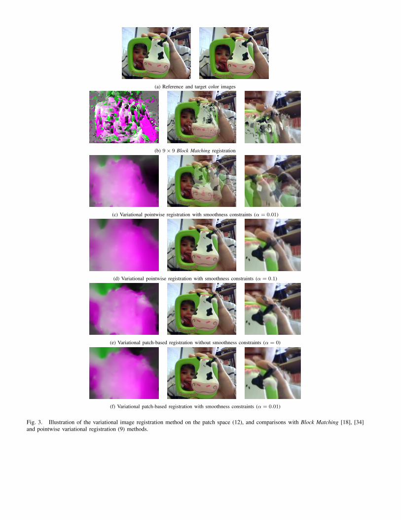
Color image registration : The patch-based registration PDE’s (12) allow to estimate a smooth

displacement field between two color images while considering a patch-based dissimilarity measure. Such

a displacement field can be used then to generate a morphing video sequence, where new synthetic

frames are added between the reference and target images (i.e.a re-timing process, where the reference

frame corresponds to t = 0 and the target to t = 1). Fig.3 shows a comparison of the re-timed resultsobtained by our proposed registration method (12) and by the most related ones, i.e.the Block Matching

algorithm and the pointwise version (10) of the variational registration technique (9). For each method, the

estimated displacement field u is displayed as a colored image (first column). The mid-interpolated frame

(i.e.reconstructed at t = 0.5) and a zoomed part of it are shown on the two last columns. This is indeedthe hardest frame to reconstruct since it classically exhibits the largest ghosting artefacts due to motion

estimation errors. To be able to handle large displacements, we considered a classical multiscale evolution

scheme for the PDE’s that minimize the pointwise and patch-based versions of the energy functional (9).

Without any surprise, the original Block Matching algorithm fails in reconstructing a smooth motion field,

resulting in a unpleasant mid-interpolated frame reconstruction. The pointwise version of the variational

registration technique (9) is quite competitive when the smoothness constraint is high enough (α = 0.1), butfails otherwise. Surprisingly, our proposed patch-based variational formulation (9) with the dissimilarity

measure (11) outputs a quite good reconstructed frame, even when α = 0. Considering a patch-baseddissimilarity measure seems to have a natural tendency to intrinsically regularize the registration problem.

Anyway, best visual results are obtained with our variational patch-based registration method while

considering regularization constraints on the displacement field u (last row).

VI. CONCLUSIONS & PERSPECTIVES

In this paper, a reversible patch-based transform of multi-valued images has been presented. More

important, we illustrated the fact that considering variational methods in the corresponding patch space is

a very nice way of designing the natural patch-based counterparts of classical image processing techniques.

The obtained experimental results seems to confirm this impression. We strongly believe that this effort is

a first step in reconciling both patch and variational worlds and that our proposed framework can be used

to translate many other “pointwise” variational formulations into their natural patch-based counterparts.

We will proceed on this way for future investigations.

REFERENCES

[1] Ashikhmin, M.: Synthesizing Natural Textures. Symposium on Interactive 3D Graphics. p.217–226, 2001.

[2] Ashikhmin, M.: Fast Texture Transfer. IEEE Computer Graphics and Applications, Vol.23 (4), p.38–43, 2003.

[3] Aubert, G., Kornprobst, P.: Mathematical Problems in Image Processing: PDE’s and the Calculus of Variations. Applied Mathematical

Sciences, Vol. 147, Springer-Verlag, 2006.

[4] Azzabou, N., Paragios, N., Guichard, F., Cao, F.: Variable bandwidth image denoising using image-based noise models. IEEE CVPR,

2007.

[5] Baker, S., Matthews, I.: Lucas-Kanade 20 Years On: A Unifying Framework. International Journal of Computer Vision, Vol.56 (3),

p.221–255, 2004.

[6] Barash, D.: A fundamental relationship between bilateral filtering, adaptive smoothing, and the nonlinear diffusion equation. IEEE

PAMI, Vol.24 (6), p.844–847, 2002.

[7] Barash, D., Comaniciu, D.: A common framework for Nonlinear Diffusion, Adaptive Smoothing, Bilateral Filtering and Mean Shift.

Image Vision Comp., Vol.22 (1), 2004.

(a) Noisy image (std=20) (b) Tikhonov regularization on Ω (c) Bilateral Filtering (d) Non Local Means

Result PSNR Parameters Reference

(b) 25.33 dB σ = 0.6 [10], [30]

(c) 26.97 dB σs = 10, σr = 25 [6], [26], [31]

(d) 26.98 dB σ = 21, patch 7 × 7 [13]

(e) 27.03 dB σ = 21, patch 7 × 7 .

(e) Tikhonov regularization on the patch space Γ (f) PSNR(Original/Denoised) and parameters used for experiments

Fig. 1. Illustration of the Tikhonov regularization on the patch space (7), and comparisons with most related filtering techniques.

[8] Bertalmıo, M., Sapiro, G., Caselles, V., Ballester, C.: Image inpainting. SIGGRAPH, Computer Graphics Proceedings, p.417–424, 2000.

[9] Bertalmıo, M., Vese, L.A., Sapiro, G., Osher, S.: Simultaneous Structure and Texture Image Inpainting. IEEE CVPR, p.707–712, 2003.

[10] Bouhamidi, A., Jbilou, K.: Sylvester Tikhonov-Regularization Methods in Image Restoration. J. Comput. Appl. Math. Vol.206 (1),

p.86–98, 2007.

[11] Boulanger, J., Kervrann, C., Bouthemy, P.: Space-time Adaptation for Patch-based Image Sequence Restoration. IEEE PAMI. Vol.29

(6), p.1096–1102, 2007.

[12] Brox, T., Cremers, D.: Iterated Nonlocal Means for Texture Restoration. SSVM. Vol.4485 of Lecture Notes in Computer Science,

Springer p.13–24, 2007.

[13] Buades, A., Coll, B., Morel, J.M.: A Non-Local Algorithm for Image Denoising. IEEE CVPR, p.60–65, 2005.

[14] Criminisi, A., Perez, P., Toyama, K.: Region Filling and Object Removal by Exemplar-based Image Inpainting. IEEE Transactions on

Image Processing, Vol.13 (9), p.1200–1212, 2004.

[15] Zenzo, S.D.: A Note on the Gradient of a Multi-image. Computer Vision, Graphics, and Image Processing, Vol.33 (1), p.116–125,

1986.

[16] Efros, A.A., Leung, T.K.: Texture Synthesis by Non-Parametric Sampling. IEEE ICCV, Vol.2, p.1033–1038, 1999.

[17] Fadili, M., Starck, J.L., Boubchir, L.: Morphological Diversity and Sparse Image Denoising. IEEE ICASSP, Vol.1, p.589–592, 2007.

[18] Haworth, C., Peacock, A.M., Renshaw, D.S.: Performance of Reference Block Updating Techniques when Tracking with the Block

Matching Algorithm. IEEE ICIP, Vol.1, p.365–368, 2001.

[19] Hays, J., Efros, A.A.: Scene Completion using Millions of Photographs. ACM Trans. Graph., Vol.26 (3), 2007.

[20] Hertzmann, A., Jacobs, C.E., Oliver, N., Curless, B., Salesin, D.: Image Analogies. SIGGRAPH, Computer Graphics Proceedings,

p.327–340, 2001.

[21] Kervrann, C., Boulanger, J.: Optimal Spatial Adaptation for Patch-based Image Denoising. IEEE Transactions on Image Processing,

Vol.15 (10), p.2866–2878, 2006.

[22] Kindermann, S., Osher, S., Jones, P.: Deblurring and Denoising of Images by Nonlocal Functionnals. SIAM Multiscale Modeling and

Simulation, Vol.4, p.1091–1115, 2005.

(a) Original degraded image (b) Tikhonov regularization on the patch space Γ

(a) Original degraded image (b) Using anisotropic diffusion PDE’s [32] (c) Using Tikhonov on the patch space Γ

Fig. 2. Additional results obtained by the Tikhonov regularization flow on the patch space (7).

[23] Koenderink, J.: The Structures of Images. Biological Cybernetics, Vol.50, p.363–370, 1984.

[24] Lucas, B.D., Kanade, T.: An Iterative Image Registration Technique with an Application to Stereo Vision. Hayes, P.J., Ed.: IJCAI,

William Kaufmann, p.674–679, 1981.

[25] Osher, S., Sole, A., Vese, L.: Image Decomposition and Restoration using Total Variation Minimization and the H-1 Norm. UCLA

CAM Report, Vol.57, 2002.

[26] Paris, S., Durand, F.: A Fast Approximation of the Bilateral Filter using a Signal Processing Approach. ECCV Vol.3954 (4), LNCS,

Springer, p.568–580, 2006.

[27] Peyre, G.: Manifold Models for Signals and Images. Research Report, Ceremade, 2007-14. (2007)

[28] Sapiro, G.: Geometric Partial Differential Equations and Image Analysis. Cambridge University Press, 2001.

[29] Sochen, N.A., Zeevi, Y.Y.: Representation of Colored Images by Manifolds Embedded in Higher Dimensional Non-Euclidean Space.

ICIP, Vol.1, p.166–170, 1998.

[30] Tikhonov, A.: Regularization of Incorrectly Posed Problems. Soviet Math. Vol.4, p.1624–1627, 1963.

[31] Tomasi, C., Manduchi, R.: Bilateral Filtering for Gray and Color images. ICCV. p.839–846, 1998.

[32] Tschumperle, D., Deriche, R.: Vector-valued Image Regularization with PDE’s: A Common Framework for Different Applications.

IEEE PAMI, Vol.27 (4), p.506–517, 2005.

[33] Wei, L.Y., Levoy, M.: Fast Texture Synthesis using Tree-structured Vector Quantization. SIGGRAPH, Computer Graphics Proceedings,

p.479–488, 2000.

[34] Wiegand, T., Sullivan, G., Bjntegaard, G., Luthra, A.: Overview of the H264 Video Coding Standard. IEEE Trans. on Circuits and

Systems for Video Tech., 13(7), p.560–576, 2003.

(a) Reference and target color images

(b) 9 × 9 Block Matching registration

(c) Variational pointwise registration with smoothness constraints (α = 0.01)

(d) Variational pointwise registration with smoothness constraints (α = 0.1)

(e) Variational patch-based registration without smoothness constraints (α = 0)

(f) Variational patch-based registration with smoothness constraints (α = 0.01)

Fig. 3. Illustration of the variational image registration method on the patch space (12), and comparisons with Block Matching [18], [34]

and pointwise variational registration (9) methods.