1 Day 1 - Session 2 Camera Calibration Calibration Principles • Collinearity assumes the camera produces a perfect central projection • The fundamental parameters required are the principal distance and the location of the principal point • Small departures from the perfect central projection must be modelled to avoid systematic errors • The significant effects are lens distortions and image deformations
Transcript
1
Day 1 - Session 2
Camera Calibration
Calibration Principles• Collinearity assumes the camera produces a perfect central projection
• The fundamental parameters required are the principal distance and the location of the principal point
• Small departures from the perfect central projection must be modelled to avoid systematic errors
• The significant effects are lens distortions and image deformations
2
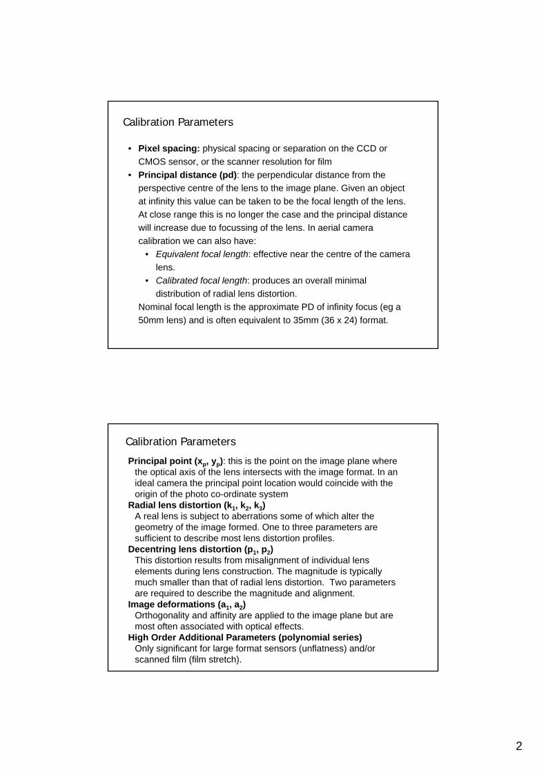
• Pixel spacing: physical spacing or separation on the CCD or CMOS sensor, or the scanner resolution for film
• Principal distance (pd): the perpendicular distance from the perspective centre of the lens to the image plane. Given an object at infinity this value can be taken to be the focal length of the lens. At close range this is no longer the case and the principal distance will increase due to focussing of the lens. In aerial camera calibration we can also have:
• Equivalent focal length: effective near the centre of the camera lens.
• Calibrated focal length: produces an overall minimal distribution of radial lens distortion.
Nominal focal length is the approximate PD of infinity focus (eg a 50mm lens) and is often equivalent to 35mm (36 x 24) format.
Calibration Parameters
Principal point (xp, yp): this is the point on the image plane where the optical axis of the lens intersects with the image format. In an ideal camera the principal point location would coincide with the origin of the photo co-ordinate system
Radial lens distortion (k1, k2, k3)A real lens is subject to aberrations some of which alter the geometry of the image formed. One to three parameters are sufficient to describe most lens distortion profiles.
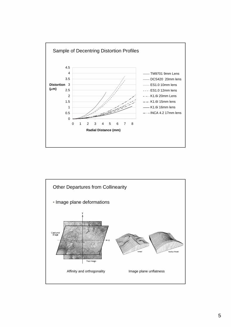
Decentring lens distortion (p1, p2)This distortion results from misalignment of individual lens elements during lens construction. The magnitude is typically much smaller than that of radial lens distortion. Two parameters are required to describe the magnitude and alignment.
Image deformations (a1, a2)Orthogonality and affinity are applied to the image plane but are most often associated with optical effects.
High Order Additional Parameters (polynomial series)Only significant for large format sensors (unflatness) and/or scanned film (film stretch).
Calibration Parameters
3
Lens Distortions
• Radial and decentring lens distortion
Effect of Radial Distortion
Caused by the design compromise between image quality and image geometry
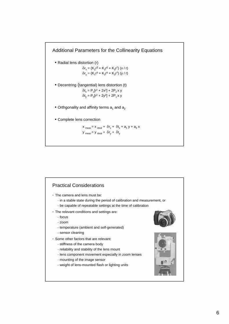
• Decentring (tangential) lens distortion (t)δtx = P1[r2 + 2x2] + 2P2 x yδty = P2[r2 + 2y2] + 2P1 x y
• Orthgonality and affinity terms a1 and a2
• Complete lens correction
x meas = x ideal + δrx + δtx + a1 y + a2 xy meas = y ideal + δry + δty
Additional Parameters for the Collinearity Equations
Practical Considerations
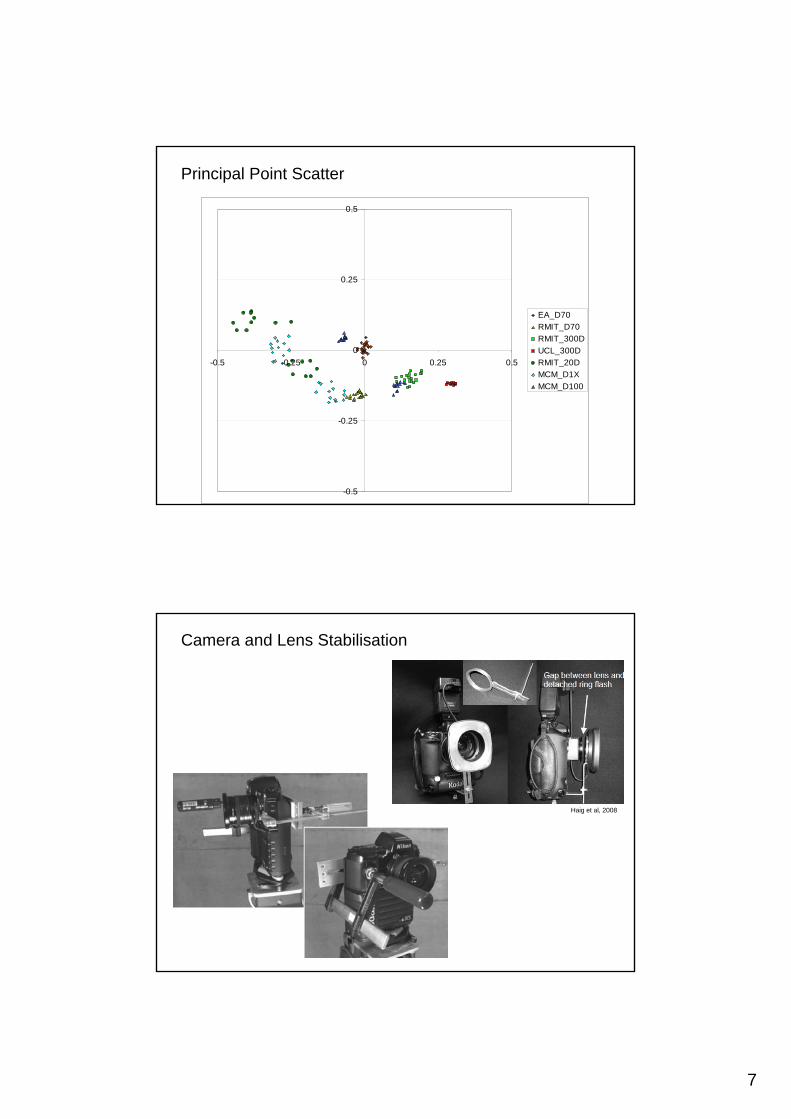
• The camera and lens must be:– in a stable state during the period of calibration and measurement, or– be capable of repeatable settings at the time of calibration
• The relevant conditions and settings are:– focus– zoom– temperature (ambient and self-generated)– sensor cleaning
• Some other factors that are relevant:– stiffness of the camera body– reliability and stability of the lens mount– lens component movement especially in zoom lenses– mounting of the image sensor– weight of lens-mounted flash or lighting units
The mathematical parameter sets describing the geometry of a camera system can be determined through a variety of different methods
• Laboratory calibrations where one or more properties of a camera system are investigated under carefully controlled conditions. The approach usually involves component analysis and optical techniques such as collimators.
• Target array or test range calibration where a 3D array of targets is imaged from multiple viewpoints and parameters of camera interior orientation are computed using network adjustment techniques.
• Plumb line calibration where the imaged distortions of an array of lines known to be straight in the object space are used to compute parameters of radial and decentring lens distortion.
Laboratory Calibration
Clarke and Fryer 1995
9
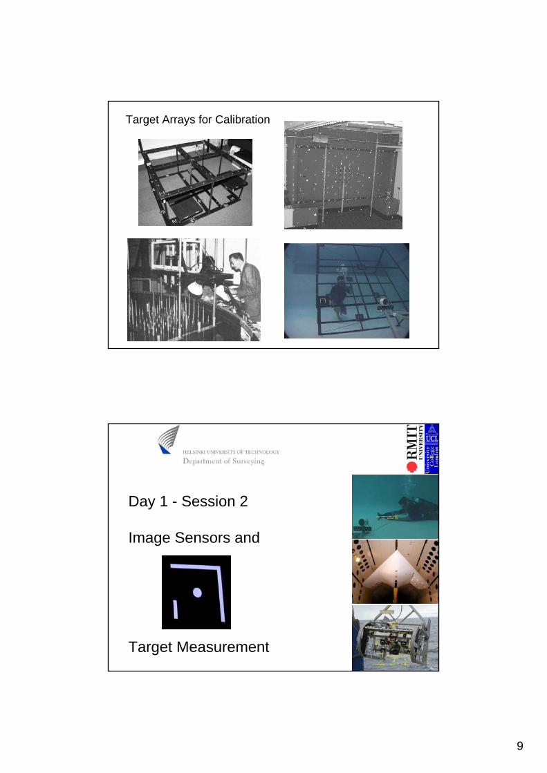
Target Arrays for Calibration
Day 1 - Session 2
Image Sensors and
Target Measurement
10
Light photons incident on the sensor material are collected to produce an electrical signal at each pixel
Analog image voltage and timing signals produced by reading the signal produced at each pixel in turn.
Analog image signal quantised into individual pixels by analogue to digital converter
Digital image data in computer readable form
Distance
IA/D
Converter(typically 8 bit, but 10, 12 16 and 32 bits possible)
Distance
gv
0
255Analog signal Digital representation
Digital Image Acquisition
Two principal types of image sensor• Interline transfer is derived from the TV
and broadcast standards where the array produces an interlaced image to minimise the quantity of data transmitted whilst maintaining the 25 frames per second necessary to avoid perceptible image flicker.
– Method is limited in that the odd and even lines represent two different periods in time
• Frame transfer sensors are organised such that the light sensitive regions are also used to transfer charge and the image is read-out as a single frame.
– Method depends on an independent storage and readout zone or a mechanical shutter to prevent light reaching the sensor whilst the image information is read out.
• Progressive scan sensors are a specific type of frame transfer
SensorElement
Row Bus
Column Bus
Horizontal Scan Register
Vertical Scan Register
OutputAmplifier
Video Out
Digital Image Sensors (CCD and CMOS)
11
Bucket Array Analogy
Photons
Gauge
Conveyors
Conveyor
Sensor Characteristics
• Format size, pixel spacing and fill factor (the amount of each pixel that is sensitive to light) vary tremendously
• Smaller format or low fill factor = smaller pixels = less photons = less sensitivity = higher amplification = more noise
• 3 sensor (RGB) cameras have higher image quality
Wikipedia
12
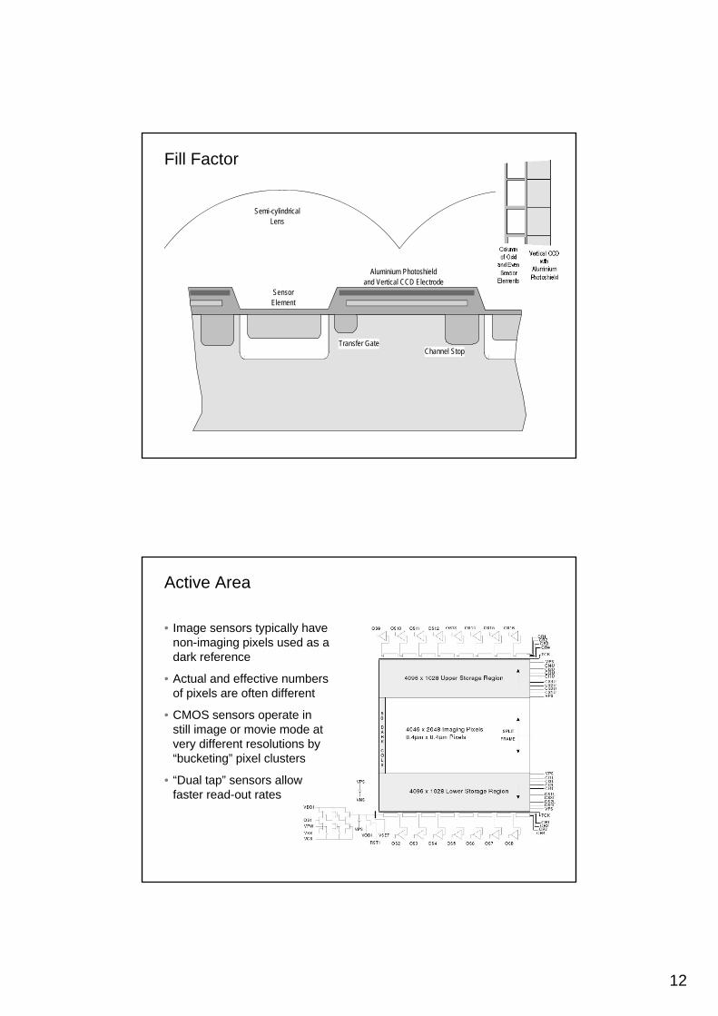
Fill Factor
Semi-cylindricalLens
SensorElement
Aluminium Photoshieldand Vertical CCD Electrode
Channel StopTransfer Gate
Active Area
• Image sensors typically have non-imaging pixels used as a dark reference
• Actual and effective numbers of pixels are often different
• CMOS sensors operate in still image or movie mode at very different resolutions by “bucketing” pixel clusters
• “Dual tap” sensors allow faster read-out rates
13
Colour: Bayer colour filter arrays
• Common method for capturing colour imagery from single CCD cameras
• Reduces camera size and cost RG RG
B G B G
R G
B G
RG RG
B G B G
R G
B G
RG RG
B G B G
R G
B G
• Each pixel is made sensitive to either R, G, or B
• Green is dominant to maximise luminance information
• Full-colour image is obtained by interpolating missing colours
It is conventional for a photogrammetric image coordinate system to have an origin at the centre of the image format, coinciding with the optical axis of the lens in an ideal central perspective projection. Image sensor arrays are highly regular structures, which given consistent electronic signal timing, provide an excellent image coordinate system.
x photo co-ordinate axis
y photo co-ordinate axistrue origin
Y pixel axis(0,0)
(0,0)
Digital image
Y pixel size
X pixel sizefalse origin
X pixel axisHowever, the sensor scanning process conventionally reads from the top left corner of the array, line by line, towards the bottom right corner. A simple 2D transformation is therefore necessary to obtain the familiar photo coordinate system.
Image Coordinate Systems
14
Sub-pixel Location of a Retro-reflective Target Image on a Dark Background
Pixel Value
Threshold
Pixel Value
Pixel Value
Pixel Number
Pixel Number
Centroid
Sub pixel location
T
0
00
255
255 255
Intensity
A/D conversion
Thresholds
• Thresholds are used for the full image during image scanning or in a local image patch or window to compute the target image centroid
• Three threshold types are commonly used:–histogram based threshold that assumes the full image or image
window contains a bi-polar distribution–statistical (mean plus n standard deviations) threshold extracted
from the edges of the window or image patch–fixed threshold specified by the operator or set heuristically
15
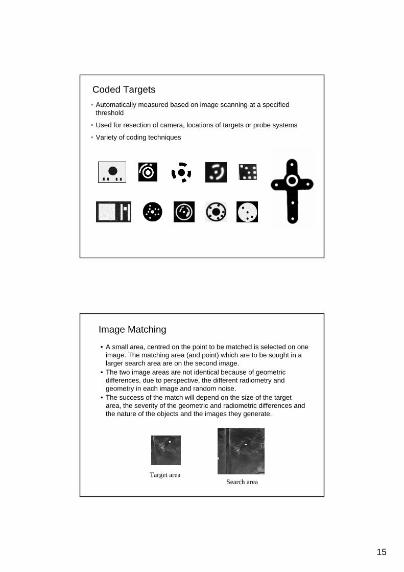
Coded Targets• Automatically measured based on image scanning at a specified
threshold
• Used for resection of camera, locations of targets or probe systems
• Variety of coding techniques
• A small area, centred on the point to be matched is selected on one image. The matching area (and point) which are to be sought in alarger search area are on the second image.
• The two image areas are not identical because of geometric differences, due to perspective, the different radiometry and geometry in each image and random noise.
• The success of the match will depend on the size of the target area, the severity of the geometric and radiometric differences and the nature of the objects and the images they generate.
Image Matching
Target areaSearch area
16
Transformation of an Image Patch
Based on an affine 2D transformation within the image space
Geometrically Constrained Multi-photo Adaptive Least Squares Matching
4 images, starting position
Solution with geometric constraints
Solution without geometric constraints
17
Day 1 - Session 2
Photogrammetric Networks
Basic Concepts and Terminology (1)
• Accuracy: closeness to the truth (what is the truth?)
• Reliability: ability to detect all types of errors in measurements
• Precision or Uncertainty: spread of a measurement set, usually stated in terms of standard deviation or Root Mean Square (RMS) error
Wikipedia (2008)
18
Basic Concepts and Terminology (2)
• Systematic error: caused by an un-modelled effect in the measurements
• Gross error, blunder: mistake in the data, usually caused by human error or equipment failure
• Mean: average value of a set of random, independent measurements
Wikipedia (2008)
• Normal or Gaussian distribution: standard “bell” curve of random, independent measurements distributed around a mean
• Least Squares Estimation: computation technique based on minimisation of the sum of the squares of the random errors in measurements
Basic Concepts and Terminology (3)
• Confidence: probability that a random measurement falls within a specified range (eg 1-sigma contains 68.2% of the normal distribution, 2- and 3-sigma correspond to 95% and 99.7% respectively)
• Tolerance: limit of all possible randomly distributed measurements, often adopted as 5-sigma
www.cs.princeton.edu (2009)
19
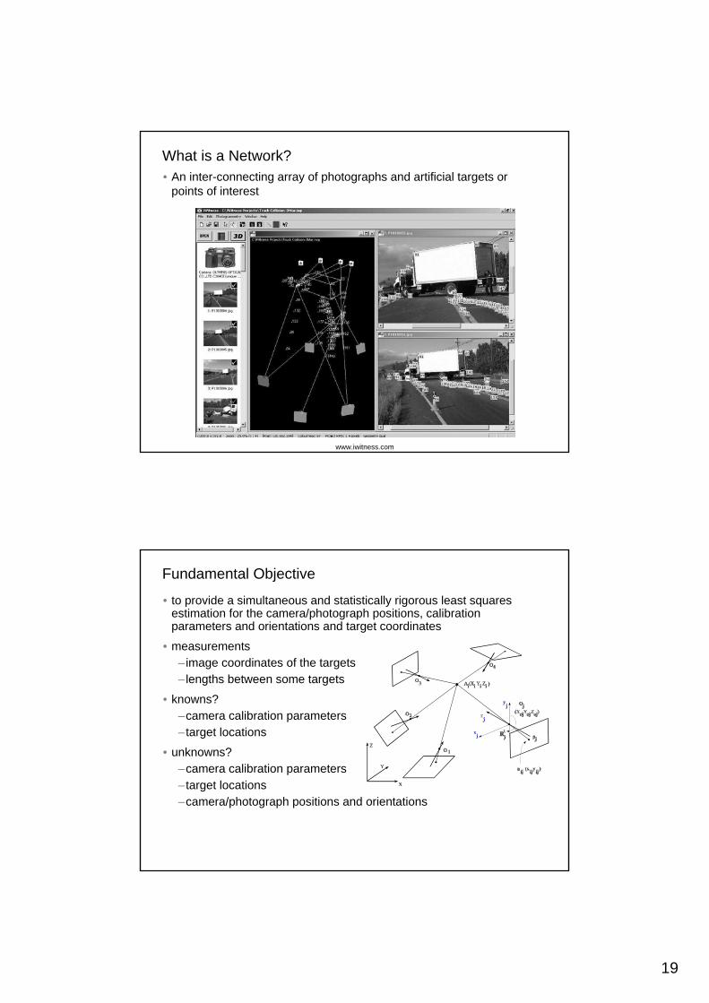
What is a Network?• An inter-connecting array of photographs and artificial targets or
points of interest
www.iwitness.com
Fundamental Objective
• to provide a simultaneous and statistically rigorous least squares estimation for the camera/photograph positions, calibration parameters and orientations and target coordinates
• measurements –image coordinates of the targets–lengths between some targets
• unknowns? –camera calibration parameters–target locations–camera/photograph positions and orientations
20
Network Geometry
• Networks can be broken down into components such as resection of photos and intersection of targets
• There must be more measurements than unknown parameters
• Networks can be externally constrained by control targets with known coordinates: three targets with seven known coordinates is the minimum requirement, also known as minimal constraints
• Networks can be internally constrained by the network solution algorithm, also known as a free network
• A strong geometrical configuration to confer the greatest accuracy and precision requires that multiple, convergent images are madefrom different locations with the same camera and that each image is able to provide measurable target images of as many targets as possible.
• If the network geometry is appropriate it is possible to include camera calibration parameters. This technique is known as self calibration.
Resection
Determination of the position and orientation of the camera. Also known as exterior orientation.
Objective:
• to determine the least squares best estimates of six parameters describing the location of the perspective centre and pointing direction of the camera optical axis when the image was taken. Six unknown parameters: X0, Y0, Z0, ω, φ and κ.
Requirements:
• a minimum of four well distributed target points whose co-ordinates in the object space are known.
• measurements of the imaged locations of each of the four known targets in the image to be resected.
• initial approximations for the six exterior orientation parameters
• provides a pair of collinearity equations per target to give eight equations with six common unknowns.
21
Resection Configuration
OP
x
y
X
Y
Z
(Xo, Yo, Zoω,φ, κ)
(Xa, Ya, Za)
(xa, ya)
cz
Intersection
Determination of the position of targets or points of interest in the object space.
Objective:
• to determine the three co-ordinates Xa, Ya, Za of a target given a pair or more of orientated images.
Requirements:
• a minimum of two images whose exterior orientations (Xo, Yo, Zo, ω, φ and κ) have been determined by, for example, the method of resection.
• measurements of the imaged location of the target in each of the images.
• initial estimates for the co-ordinates to be estimated.
• provides a pair of collinearity equations per image to give, assuming a pair of images only, four equations with three common unknowns.
22
Intersection Configuration
Scale
Network Configurations
Rigidly connected stereo pair of cameras
Network of mechanically unconnected cameras
Scale
23
Ideal Network Geometry
Network Design Factors
• Precision is dependent on the resolution of the sensor
• Higher resolution will give better precision for the target coordinates
• Reliability is dependent on:–the number of redundant measurements–high levels of redundancy (both geometric and numerical) are
essential for high reliability
• More photographs and more targets lead to high levels of redundancy, sometimes known as hyper-redundancy
• Independence of parameters is dependent on geometry
• Correlations between parameters are reduced by strong, 3D geometry
• Accuracy is evaluated by lengths or other known dimensions in the object that have been independently determined
24
Day 1 - Session 2
VDI/VDE Guidelines
Is the data fit for purpose?
• Coordinates derived from any measurement process are of no practical value without an estimate of their quality
• Required data qualities:
– Uncertainty: describes the quality of the data set with respect to random errors
– Reliability: is concerned with the ease with which gross errors or outliers may be detected
– Accuracy: describes the quality with respect to systematic errors. Accuracy is assessed with reference to external standards, such as the inclusion of a calibrated artefact or set of scale bars in a network
• Typically uses known lengths in controlled conditions
• Independent test of scale determined by calibration
• Theory prediction is sub-millimetre for underwater stereo-video
• Actual accuracy of approximately 1mm
Comprehensive Accuracy Testing Guidelines
• VDI/VDE 2634/1 for optical 3D measuring systems proposes procedures which take into account the following points
– Image-based measurement of a large number of points– Triangulation principle– Mobility– Flexible configurations– Unlimited measuring volume
• VDI 2634/2 for area-based systems– Surface measurement on a calibrated reference sphere– Flatness measurement error– Sphere spacing error (~ ISO-conform length measurement error)
• VDI 2634/3 for systems that provide area-based measurements and sensor orientations in order to measure objects that are larger than the initial measuring volume of a surface measuring sensor
26
VDI/VDE 2634/1 Implementation
L [mm]0.00
0.05
0.10
-0.05
-0.10500 1000 1500 2000
A
A
B
B
E
E
ΔL [mm]
• Utilises the difference between a measured length and a calibrated reference length
• Maximum permitted positive and negative limit of length measurement error is defined as a length-dependent value that may not be exceeded in the checking of any deviation of length measurement
Potential sources of error in large-scale metrology systemsStability of the measurement environment
– is often the dominant source of measurement error
– differential thermal expansion within the work piece
– measurement in the presence of vibration– differential heating of the instrument – optical refraction– mechanical vibration of the instrument
magnified over long path lengths
Measurement EnvironmentMeasurement Environment
UserUser
InstrumentationInstrumentationWorkpieceWorkpiece
In addition large systematic errors and blunders can arise at the interface between each of these components.
For example the user may set incorrect parameters in the instrumentation or measure the incorrect surfaces on the work piece or use a target of an incorrect or inappropriate dimension.
Operational guidelines should take account of the environment in which the systems are to be deployed and take steps to control environmental conditions to bring them within acceptable limits.
27
VDI/VDE: Q-Foto System Accuracy ValidationAutomated quality control system for manufacture of solar concentrators
VDI/VDE: Q-Foto System Accuracy Validation
• Certified according to the German technical rule VDI/VDE 2634
• Carbon fibre rods used in the volume of 12m x 6m x 1.5m
• Rod lengths measured to ±0.05mm with a laser doppler displacement meter
• Initial results indicate a uncertainty of ±0.1mm and a maximum error of ±0.4mm