51
STAN WORKSHOP DAY 2

STAN WORKSHOPDAY 2

RECAP

RECAP
▸ Ran multiple Stan programs!
▸ Wrote multiple Stan programs.Non-analytic; can only be solved with MCMC.Last model isn’t found in any package.
▸ Started learning a new language.We conflated statistical modeling and the language.Stan language is really flexible. For learning: Time helps. Practice helps.
TODAY: MORE ADVANCED STAN
▸ Iterate over statistical models
▸ Hierarchical models and non-centered reparameterization
▸ Exposing functions

HIERARCHICAL MODELS

8 SCHOOLS
▸ Educational Testing Service studied effect of coaching on SAT scores
▸ No prior belief any one program was
▸ more effective than the others
▸ more similar to others

8 SCHOOLS: DATA
School Estimated treatment effect
Standard error of treatment effect
A 28 15B 8 10C -3 16D 7 11E -1 9F 1 11G 18 10H 12 18

READ DATAFrom: https://github.com/stan-dev/rstan/wiki/RStan-Getting-Started
In R:
schools_dat <- list(J = 8,
y = c(28, 8, -3, 7, -1, 1, 18, 12),
sigma = c(15, 10, 16, 11, 9, 11, 10, 18))
Stan program:
data {
int J;
real y[J];
real<lower = 0> sigma[J];
}
...
MODEL 1: COMPLETE POOLING
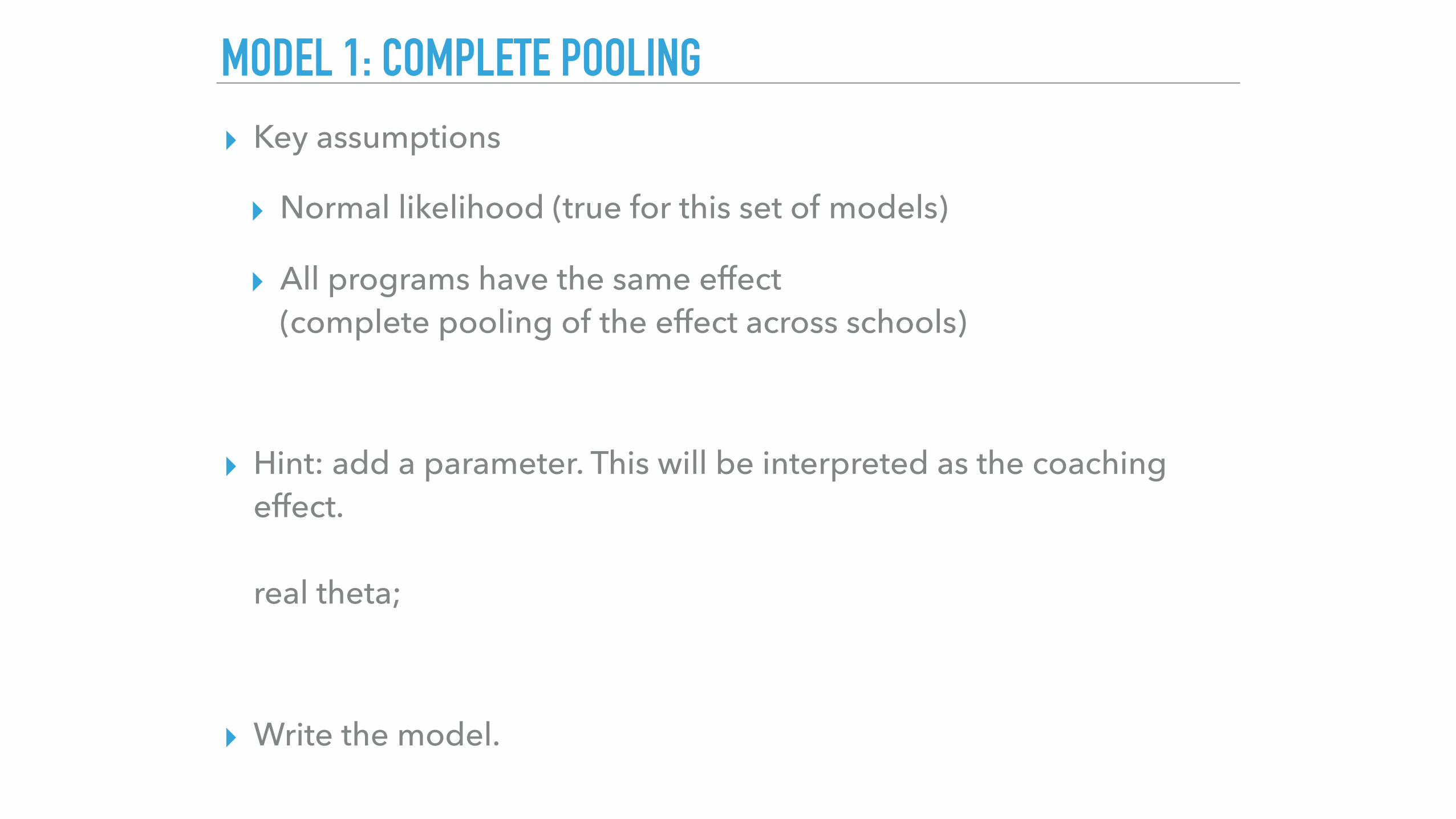
▸ Key assumptions
▸ Normal likelihood (true for this set of models)
▸ All programs have the same effect(complete pooling of the effect across schools)
▸ Hint: add a parameter. This will be interpreted as the coaching effect. real theta;
▸ Write the model.
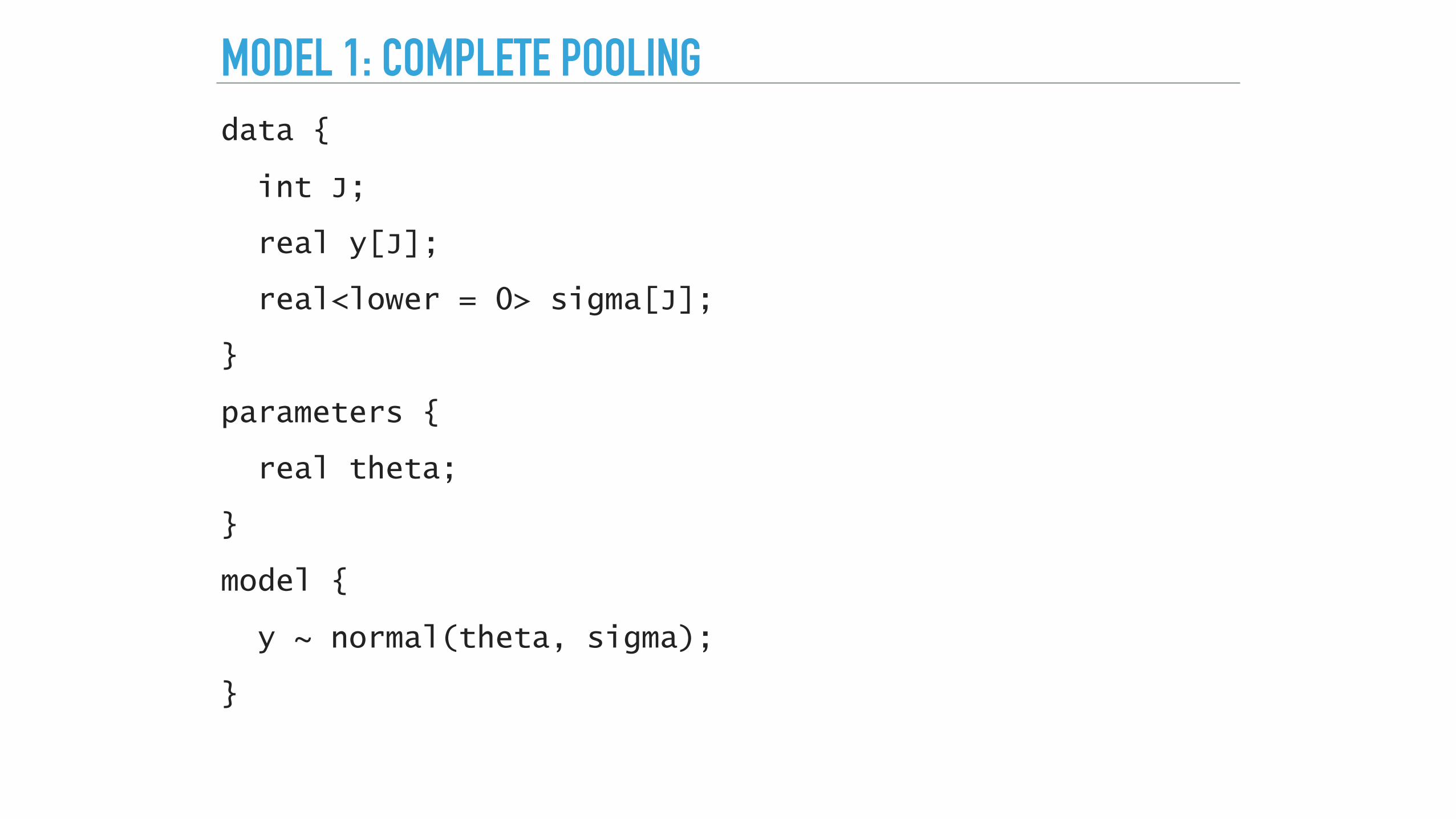
MODEL 1: COMPLETE POOLINGdata {
int J;
real y[J];
real<lower = 0> sigma[J];
}
parameters {
real theta;
}
model {
y ~ normal(theta, sigma);
}

MODEL 1: COMPLETE POOLING▸ Run using RStan
▸ fit1 <- stan(“eight_schools_1.stan", data = schools_dat)
> fit1
Inference for Stan model: eight_schools_1.
4 chains, each with iter=2000; warmup=1000; thin=1;
post-warmup draws per chain=1000, total post-warmup draws=4000.
mean se_mean sd 2.5% 25% 50% 75% 97.5% n_eff Rhat
theta 7.87 0.11 4.07 -0.24 5.22 7.94 10.62 15.74 1465 1
lp__ -2.85 0.02 0.72 -4.85 -3.02 -2.58 -2.40 -2.35 1445 1
Samples were drawn using NUTS(diag_e) at Wed Jun 1 00:57:15 2016.
For each parameter, n_eff is a crude measure of effective sample size,
and Rhat is the potential scale reduction factor on split chains (at
convergence, Rhat=1).
MODEL 2: NO POOLING
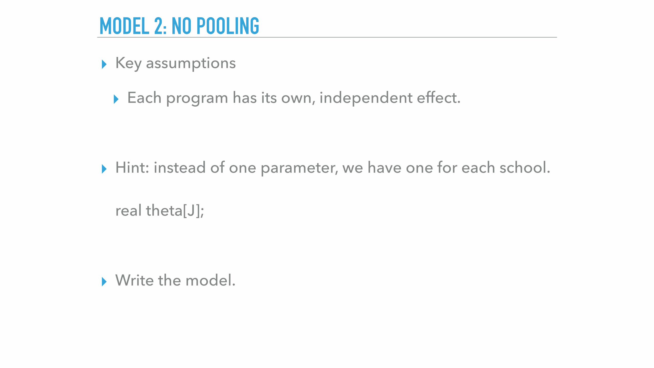
▸ Key assumptions
▸ Each program has its own, independent effect.
▸ Hint: instead of one parameter, we have one for each school. real theta[J];
▸ Write the model.

MODEL 2: NO POOLINGdata {
int J;
real y[J];
real<lower = 0> sigma[J];
}
parameters {
real theta[J];
}
model {
y ~ normal(theta, sigma);
}
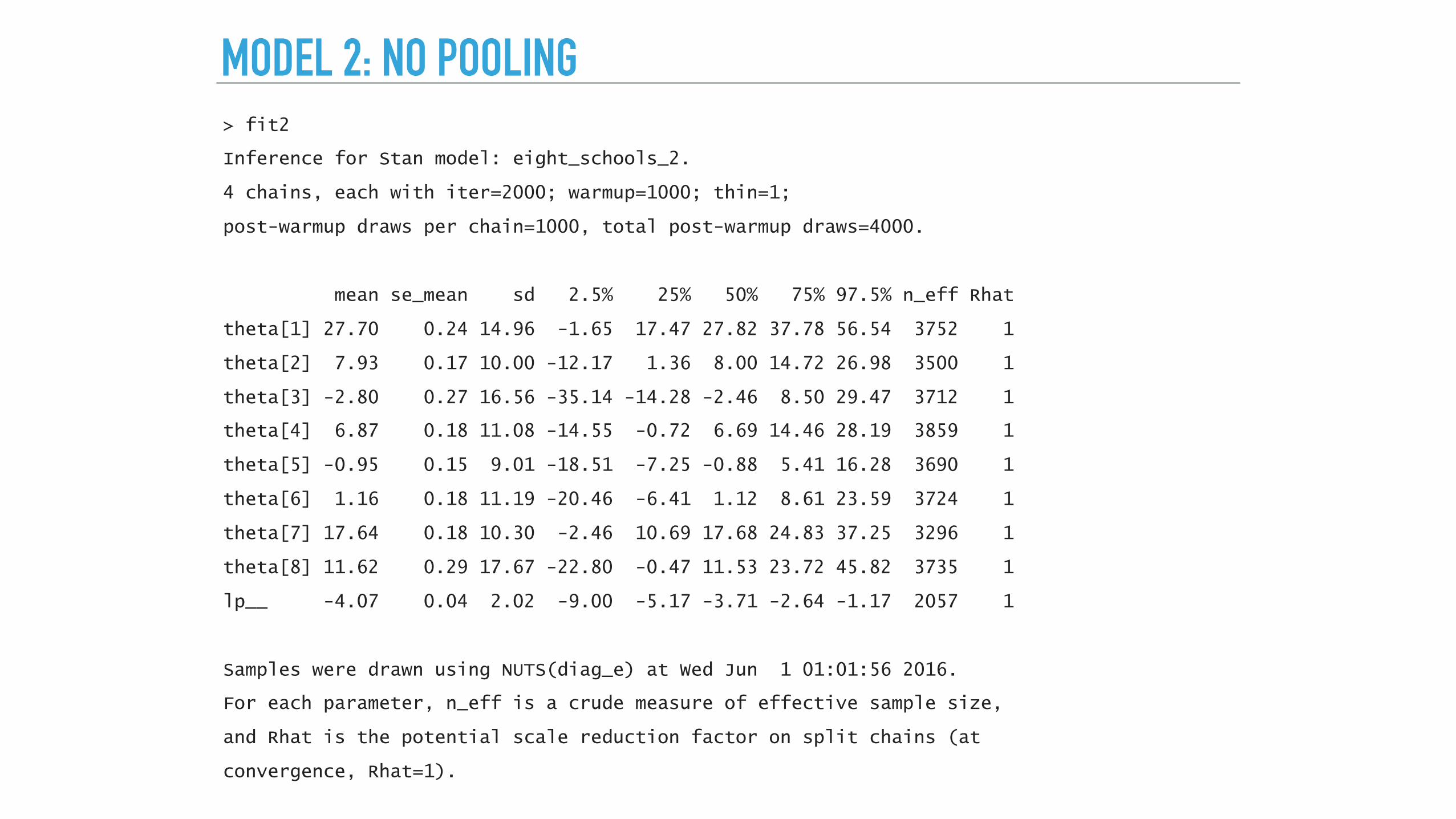
MODEL 2: NO POOLING> fit2
Inference for Stan model: eight_schools_2.
4 chains, each with iter=2000; warmup=1000; thin=1;
post-warmup draws per chain=1000, total post-warmup draws=4000.
mean se_mean sd 2.5% 25% 50% 75% 97.5% n_eff Rhat
theta[1] 27.70 0.24 14.96 -1.65 17.47 27.82 37.78 56.54 3752 1
theta[2] 7.93 0.17 10.00 -12.17 1.36 8.00 14.72 26.98 3500 1
theta[3] -2.80 0.27 16.56 -35.14 -14.28 -2.46 8.50 29.47 3712 1
theta[4] 6.87 0.18 11.08 -14.55 -0.72 6.69 14.46 28.19 3859 1
theta[5] -0.95 0.15 9.01 -18.51 -7.25 -0.88 5.41 16.28 3690 1
theta[6] 1.16 0.18 11.19 -20.46 -6.41 1.12 8.61 23.59 3724 1
theta[7] 17.64 0.18 10.30 -2.46 10.69 17.68 24.83 37.25 3296 1
theta[8] 11.62 0.29 17.67 -22.80 -0.47 11.53 23.72 45.82 3735 1
lp__ -4.07 0.04 2.02 -9.00 -5.17 -3.71 -2.64 -1.17 2057 1
Samples were drawn using NUTS(diag_e) at Wed Jun 1 01:01:56 2016.
For each parameter, n_eff is a crude measure of effective sample size,
and Rhat is the potential scale reduction factor on split chains (at
convergence, Rhat=1).

MODEL 3: PARTIAL POOLING WITH FIXED HYPERPARAMETER
▸ Key assumptions
▸ Hierarchical model on school effects:Schools are similar to each other, but not exactly the same
▸ Determined by hyperparameter, tau.
▸ Hint:
▸ add new data: real<lower = 0> tau;
▸ add new parameter: real mu;
▸ Write the model.

MODEL 3: PARTIAL POOLING WITH FIXED HYPERPARAMETERdata {
int J;
real y[J];
real<lower = 0> sigma[J];
real<lower = 0> tau;
}
parameters {
real theta[J];
real mu;
}
model {
theta ~ normal(mu, tau);
y ~ normal(theta, sigma);
}

MODEL 3: PARTIAL POOLING WITH FIXED HYPERPARAMETER, TAU = 25> fit3
Inference for Stan model: eight_schools_3.
4 chains, each with iter=2000; warmup=1000; thin=1;
post-warmup draws per chain=1000, total post-warmup draws=4000.
mean se_mean sd 2.5% 25% 50% 75% 97.5% n_eff Rhat
theta[1] 22.73 0.22 13.18 -3.10 13.91 22.82 31.46 48.13 3664 1
theta[2] 8.04 0.15 9.57 -10.27 1.58 7.94 14.39 27.30 3855 1
theta[3] 0.35 0.23 14.05 -25.89 -9.71 0.25 9.89 28.20 3826 1
theta[4] 7.32 0.16 10.09 -12.09 0.44 7.41 14.39 26.73 4000 1
theta[5] 0.05 0.14 8.60 -16.72 -5.76 -0.03 5.70 17.51 3878 1
theta[6] 2.21 0.16 10.01 -17.48 -4.63 2.23 9.07 21.46 3768 1
theta[7] 16.63 0.15 9.47 -1.92 10.37 16.58 23.05 34.67 3993 1
theta[8] 10.72 0.26 15.13 -18.11 0.39 10.60 21.09 39.70 3514 1
mu 8.63 0.17 9.93 -10.41 1.76 8.69 15.41 28.03 3496 1
lp__ -5.00 0.05 2.10 -10.06 -6.19 -4.67 -3.45 -1.83 1624 1
Samples were drawn using NUTS(diag_e) at Wed Jun 1 01:12:02 2016.
For each parameter, n_eff is a crude measure of effective sample size,
and Rhat is the potential scale reduction factor on split chains (at
convergence, Rhat=1).

MODEL 3: PARTIAL POOLING WITH FIXED HYPERPARAMETER, TAU = 0.1> fit3
Inference for Stan model: eight_schools_3.
4 chains, each with iter=2000; warmup=1000; thin=1;
post-warmup draws per chain=1000, total post-warmup draws=4000.
mean se_mean sd 2.5% 25% 50% 75% 97.5% n_eff Rhat
theta[1] 7.95 0.31 3.98 0.77 5.05 7.64 10.76 15.87 170 1.03
theta[2] 7.95 0.31 3.98 0.81 5.03 7.60 10.81 15.77 170 1.03
theta[3] 7.95 0.30 3.98 0.79 5.04 7.63 10.77 15.83 170 1.03
theta[4] 7.94 0.31 3.98 0.76 5.06 7.64 10.79 15.84 170 1.03
theta[5] 7.94 0.30 3.98 0.76 5.04 7.65 10.77 15.84 170 1.03
theta[6] 7.94 0.31 3.98 0.76 5.03 7.63 10.78 15.79 170 1.03
theta[7] 7.95 0.31 3.98 0.74 5.05 7.62 10.80 15.80 170 1.03
theta[8] 7.95 0.31 3.98 0.72 5.05 7.63 10.80 15.78 170 1.03
mu 7.95 0.31 3.98 0.75 5.02 7.60 10.77 15.82 170 1.03
lp__ -6.80 0.06 2.09 -11.84 -7.91 -6.46 -5.28 -3.69 1100 1.00
Samples were drawn using NUTS(diag_e) at Wed Jun 1 01:13:53 2016.
For each parameter, n_eff is a crude measure of effective sample size,
and Rhat is the potential scale reduction factor on split chains (at
convergence, Rhat=1).
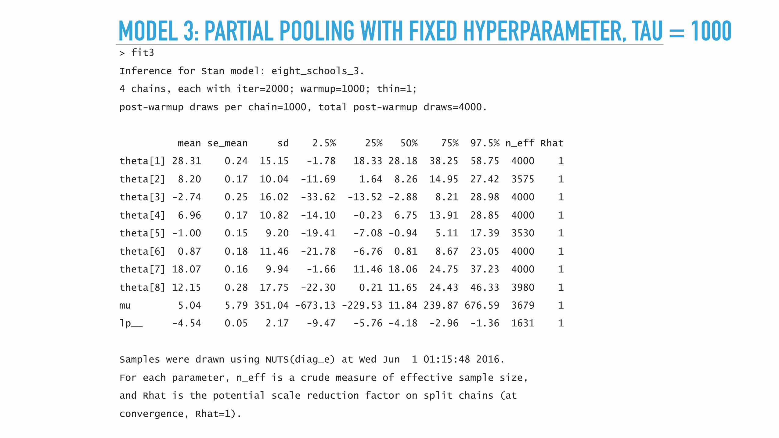
MODEL 3: PARTIAL POOLING WITH FIXED HYPERPARAMETER, TAU = 1000> fit3
Inference for Stan model: eight_schools_3.
4 chains, each with iter=2000; warmup=1000; thin=1;
post-warmup draws per chain=1000, total post-warmup draws=4000.
mean se_mean sd 2.5% 25% 50% 75% 97.5% n_eff Rhat
theta[1] 28.31 0.24 15.15 -1.78 18.33 28.18 38.25 58.75 4000 1
theta[2] 8.20 0.17 10.04 -11.69 1.64 8.26 14.95 27.42 3575 1
theta[3] -2.74 0.25 16.02 -33.62 -13.52 -2.88 8.21 28.98 4000 1
theta[4] 6.96 0.17 10.82 -14.10 -0.23 6.75 13.91 28.85 4000 1
theta[5] -1.00 0.15 9.20 -19.41 -7.08 -0.94 5.11 17.39 3530 1
theta[6] 0.87 0.18 11.46 -21.78 -6.76 0.81 8.67 23.05 4000 1
theta[7] 18.07 0.16 9.94 -1.66 11.46 18.06 24.75 37.23 4000 1
theta[8] 12.15 0.28 17.75 -22.30 0.21 11.65 24.43 46.33 3980 1
mu 5.04 5.79 351.04 -673.13 -229.53 11.84 239.87 676.59 3679 1
lp__ -4.54 0.05 2.17 -9.47 -5.76 -4.18 -2.96 -1.36 1631 1
Samples were drawn using NUTS(diag_e) at Wed Jun 1 01:15:48 2016.
For each parameter, n_eff is a crude measure of effective sample size,
and Rhat is the potential scale reduction factor on split chains (at
convergence, Rhat=1).

EFFECT OF TAU ON THETA

WOULDN’T IT BE NICE TO LEARN TAU?
▸ Amount of pooling determined by data!
▸ Easy to specify: change tau to a parameter.
▸ Problems when running:
Warning messages:
1: There were 124 divergent transitions after warmup. Increasing adapt_delta above 0.8 may help.
2: Examine the pairs() plot to diagnose sampling problems
PROBLEM: DIVERGENT TRANSITIONS
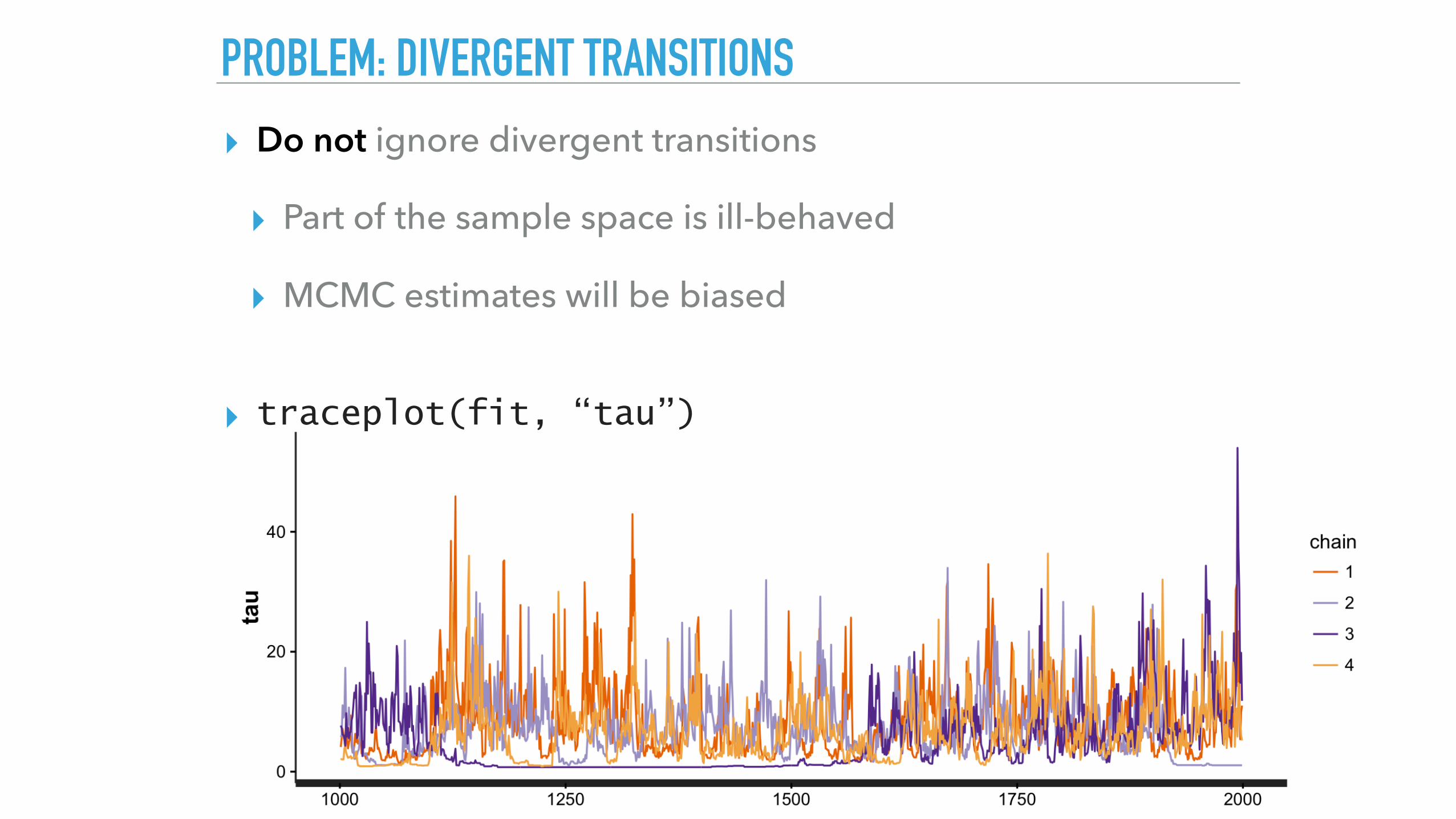
▸ Do not ignore divergent transitions
▸ Part of the sample space is ill-behaved
▸ MCMC estimates will be biased
▸ traceplot(fit, “tau”)
PROBLEM: DIVERGENT TRANSITIONS
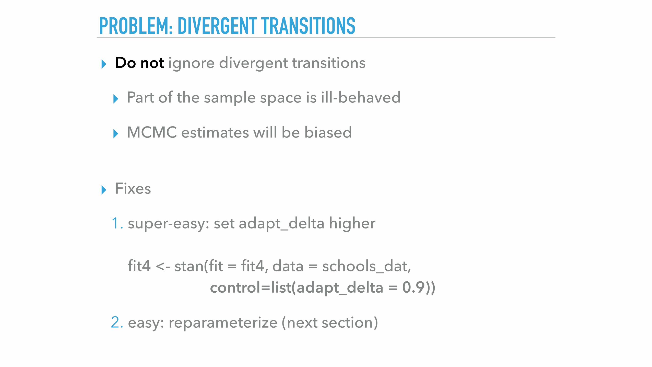
▸ Do not ignore divergent transitions
▸ Part of the sample space is ill-behaved
▸ MCMC estimates will be biased
▸ Fixes
1. super-easy: set adapt_delta higherfit4 <- stan(fit = fit4, data = schools_dat, control=list(adapt_delta = 0.9))
2. easy: reparameterize (next section)
QUICK ASIDE
▸ Why doesn’t MLE work for the hierarchical model?

QUICK ASIDE
▸ Why doesn’t MLE work for this hierarchical model?> optimizing(fit4@stanmodel, data = schools_dat)
STAN OPTIMIZATION COMMAND (LBFGS)
init = random
save_iterations = 1
init_alpha = 0.001
tol_obj = 1e-12
tol_grad = 1e-08
tol_param = 1e-08
tol_rel_obj = 10000
tol_rel_grad = 1e+07
history_size = 5
seed = 286152403
initial log joint probability = -119.833
Optimization terminated with error:
Line search failed to achieve a sufficient decrease, no more progress can be made
$par
theta[1] theta[2] theta[3] theta[4] theta[5] theta[6] theta[7] theta[8] mu tau
1.945095e+00 1.945095e+00 1.945095e+00 1.945095e+00 1.945095e+00 1.945095e+00 1.945095e+00 1.945095e+00 1.945095e+00 2.205697e-16
$value
[1] 283.0284

NON-CENTERED REPARAMETERIZATION

FUNNEL
▸
▸
y 2 R
x 2 R9
p(y, x) = Normal(y|0, 3)
⇥9Y
n=1
Normal(xn|0, exp(y/2))

WHEN DO YOU SEE THIS?
▸ Hierarchical models
▸ Variance parameters go to 0, all parameters shrink Variance parameters get large, all parameters spread
▸ Trick to handle low data situations
▸ Called non-centered parameterization aka the Matt trick ...
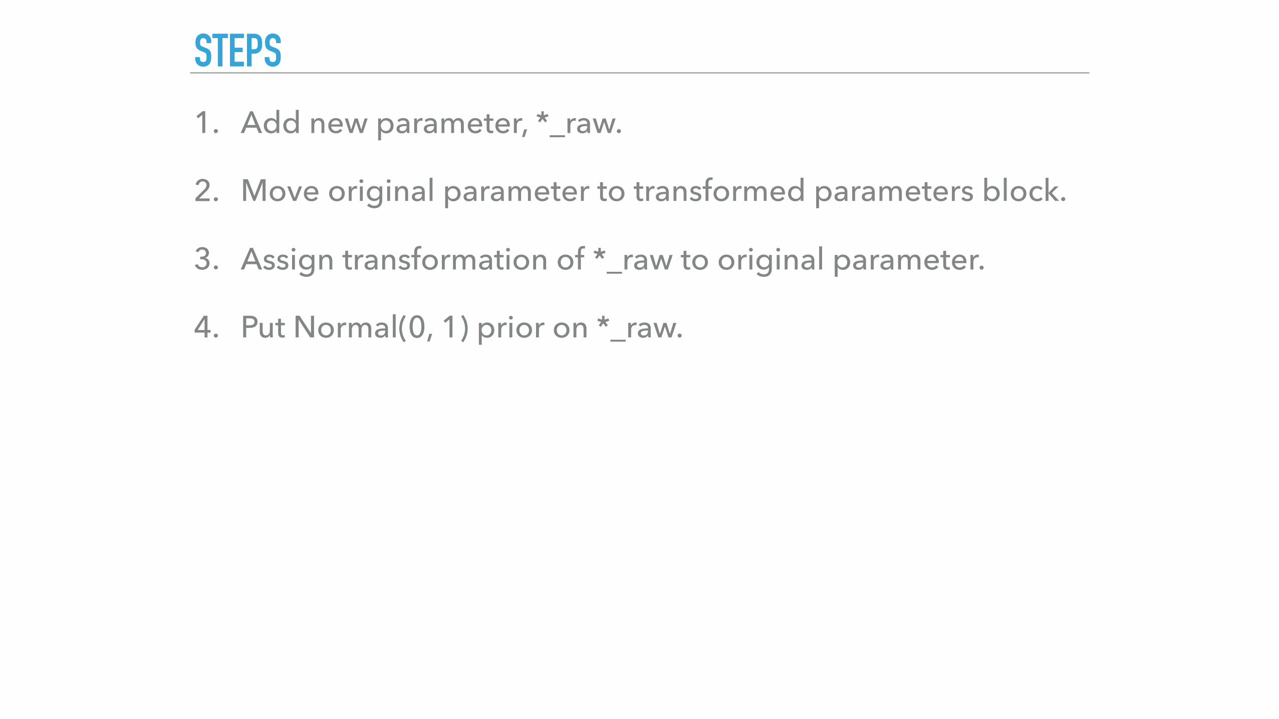
STEPS
1. Add new parameter, *_raw.
2. Move original parameter to transformed parameters block.
3. Assign transformation of *_raw to original parameter.
4. Put Normal(0, 1) prior on *_raw.
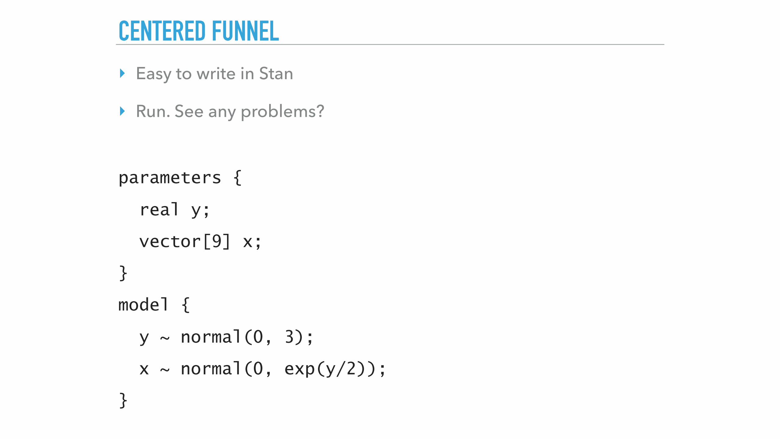
CENTERED FUNNEL
‣ Easy to write in Stan
‣ Run. See any problems?
parameters {
real y;
vector[9] x;
}
model {
y ~ normal(0, 3);
x ~ normal(0, exp(y/2));
}
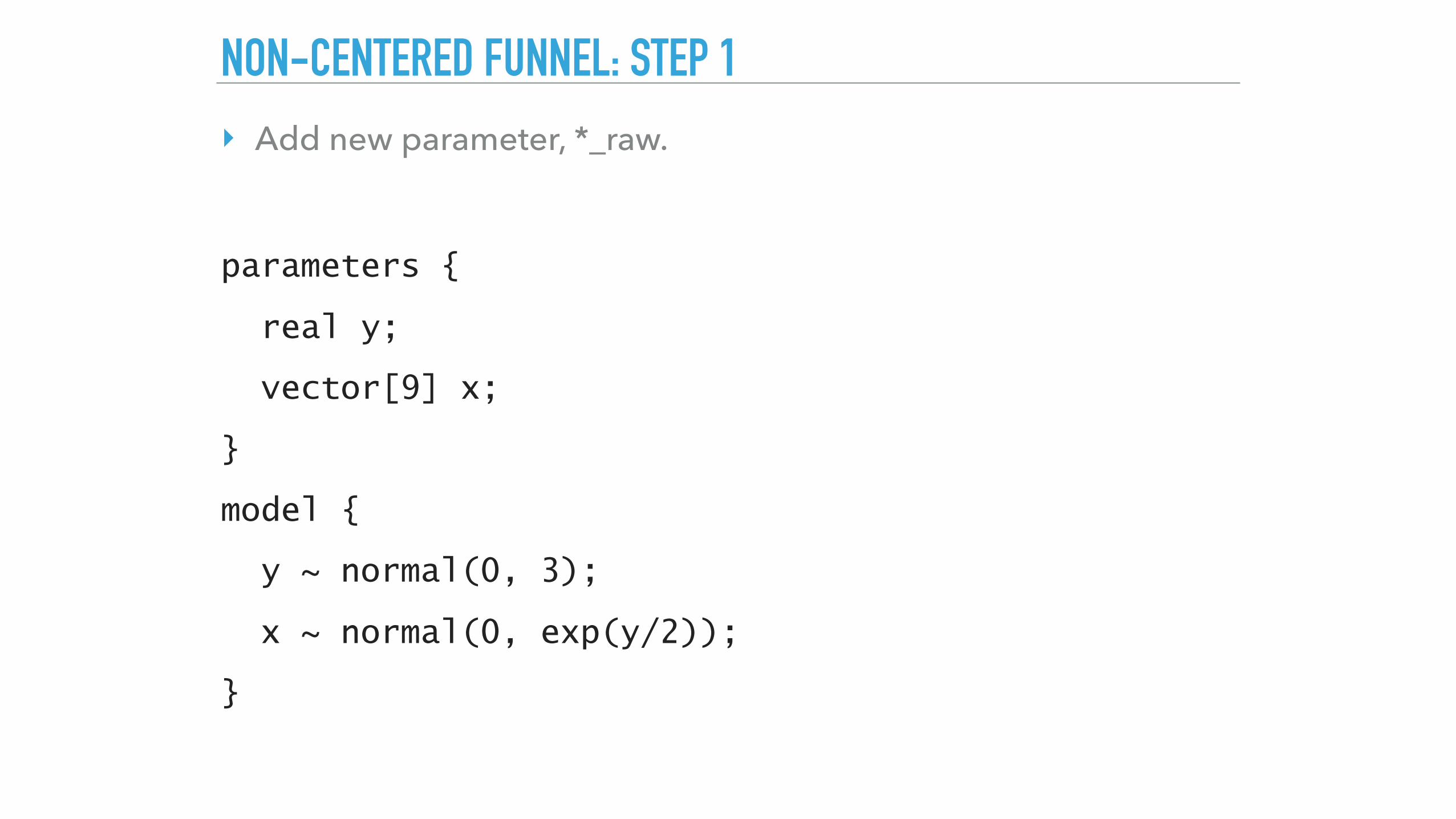
NON-CENTERED FUNNEL: STEP 1
‣ Add new parameter, *_raw.
parameters {
real y;
vector[9] x;
}
model {
y ~ normal(0, 3);
x ~ normal(0, exp(y/2));
}
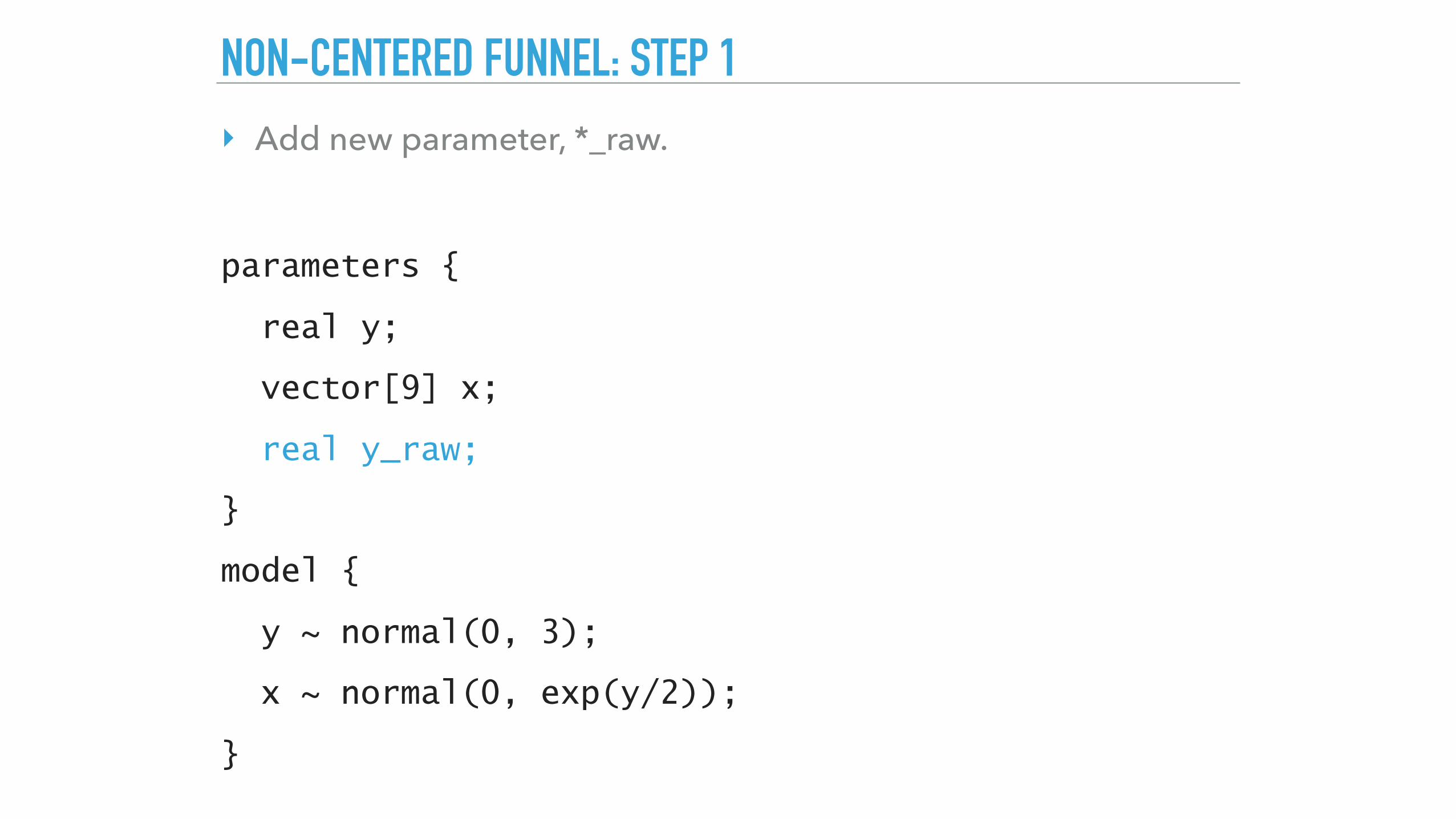
NON-CENTERED FUNNEL: STEP 1
‣ Add new parameter, *_raw.
parameters {
real y;
vector[9] x;
real y_raw;
}
model {
y ~ normal(0, 3);
x ~ normal(0, exp(y/2));
}
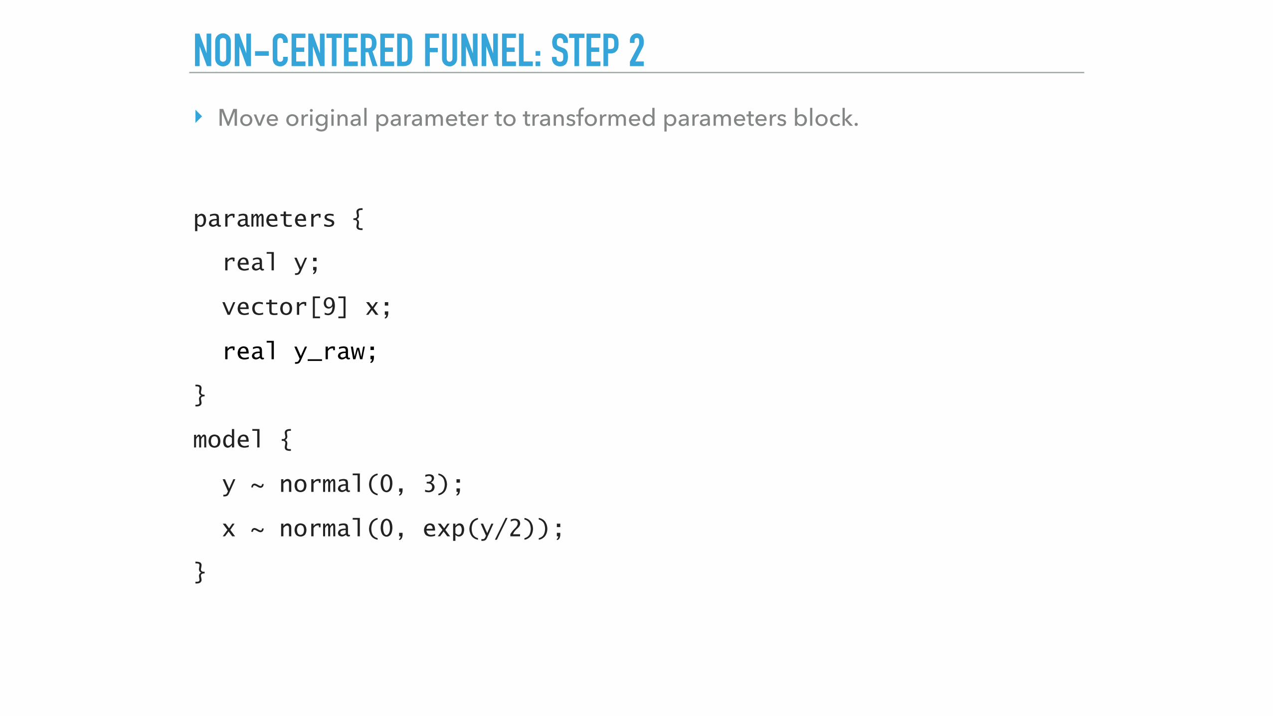
NON-CENTERED FUNNEL: STEP 2
‣ Move original parameter to transformed parameters block.
parameters {
real y;
vector[9] x;
real y_raw;
}
model {
y ~ normal(0, 3);
x ~ normal(0, exp(y/2));
}
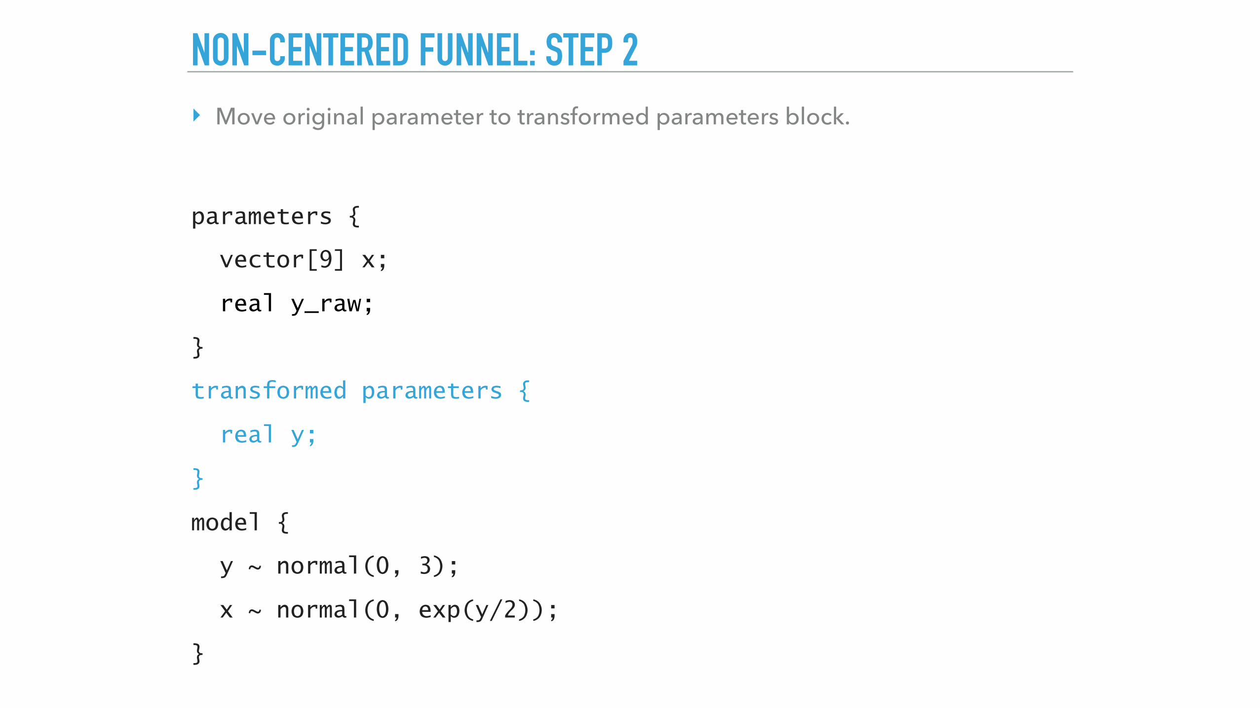
NON-CENTERED FUNNEL: STEP 2
‣ Move original parameter to transformed parameters block.
parameters {
vector[9] x;
real y_raw;
}
transformed parameters {
real y;
}
model {
y ~ normal(0, 3);
x ~ normal(0, exp(y/2));
}

NON-CENTERED FUNNEL: STEP 3‣ Assign transformation of *_raw to original parameter.
parameters {
vector[9] x;
real y_raw;
}
transformed parameters {
real y;
}
model {
y ~ normal(0, 3);
x ~ normal(0, exp(y/2));
}
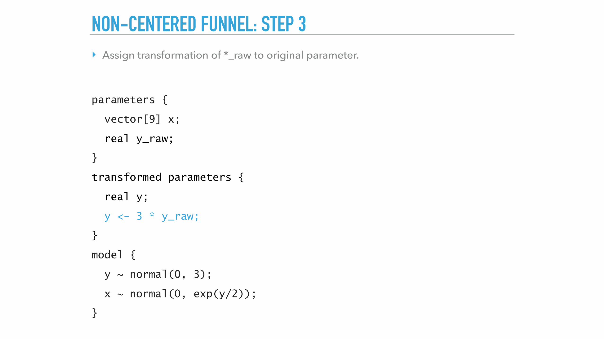
NON-CENTERED FUNNEL: STEP 3‣ Assign transformation of *_raw to original parameter.
parameters {
vector[9] x;
real y_raw;
}
transformed parameters {
real y;
y <- 3 * y_raw;
}
model {
y ~ normal(0, 3);
x ~ normal(0, exp(y/2));
}
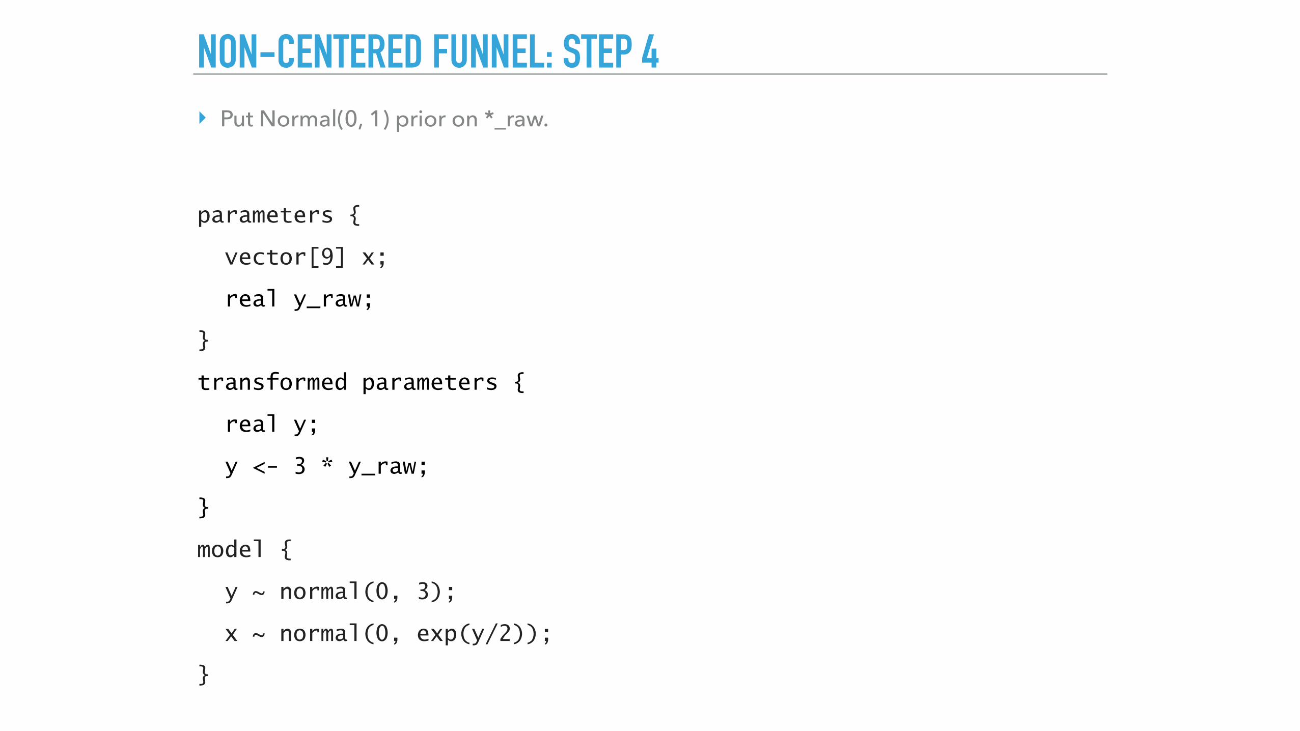
NON-CENTERED FUNNEL: STEP 4‣ Put Normal(0, 1) prior on *_raw.
parameters {
vector[9] x;
real y_raw;
}
transformed parameters {
real y;
y <- 3 * y_raw;
}
model {
y ~ normal(0, 3);
x ~ normal(0, exp(y/2));
}

NON-CENTERED FUNNEL: STEP 4‣ Put Normal(0, 1) prior on *_raw.
parameters {
vector[9] x;
real y_raw;
}
transformed parameters {
real y;
y <- 3 * y_raw;
}
model {
y_raw ~ normal(0, 1);
x ~ normal(0, exp(y/2));
}

NON-CENTERED FUNNEL
‣ Repeat for xs.
‣ Steps:
1. Add new parameter, *_raw.
2. Move original parameter to transformed parameters block.
3. Assign transformation of *_raw to original parameter.
4. Put Normal(0, 1) prior on *_raw.

NON-CENTERED FUNNELparameters {
real y_raw;
vector[9] x_raw;
}
transformed parameters {
real y;
vector[9] x;
y <- 3.0 * y_raw;
x <- exp(y/2) * x_raw;
}
model {
y_raw ~ normal(0, 1);
x_raw ~ normal(0, 1);
}
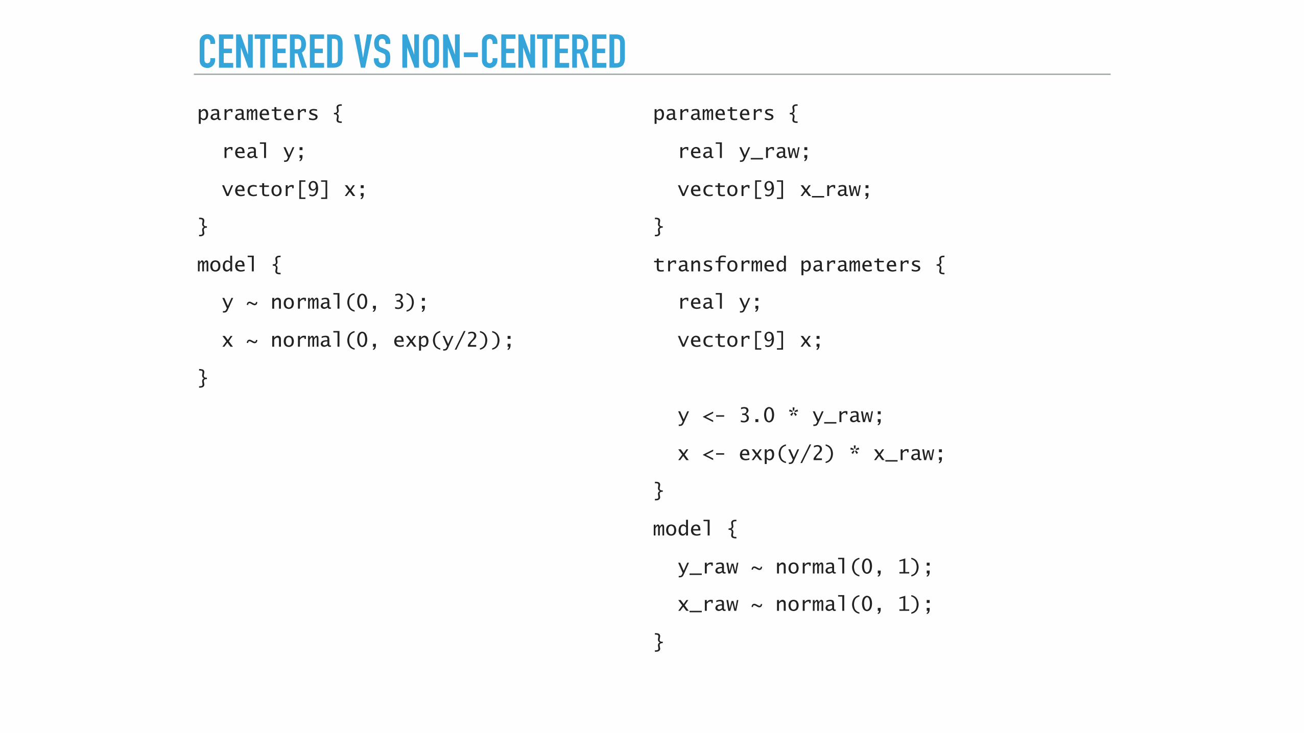
CENTERED VS NON-CENTEREDparameters {
real y;
vector[9] x;
}
model {
y ~ normal(0, 3);
x ~ normal(0, exp(y/2));
}
parameters {
real y_raw;
vector[9] x_raw;
}
transformed parameters {
real y;
vector[9] x;
y <- 3.0 * y_raw;
x <- exp(y/2) * x_raw;
}
model {
y_raw ~ normal(0, 1);
x_raw ~ normal(0, 1);
}

EIGHT SCHOOLS

REPARAMETERIZE EIGHT SCHOOLS
▸ Here’s the centered parameterization.
data { int J; real y[J]; real<lower = 0> sigma[J]; } parameters { real theta[J]; real mu; real<lower = 0> tau; } model { theta ~ normal(mu, tau); y ~ normal(theta, sigma); }

NON-CENTERED REPARAMETERIZATION
▸ Follow steps:
1. Add new parameter, *_raw.
2. Move original parameter to transformed parameters block.
3. Assign transformation of *_raw to original parameter.
4. Put Normal(0, 1) prior on *_raw.
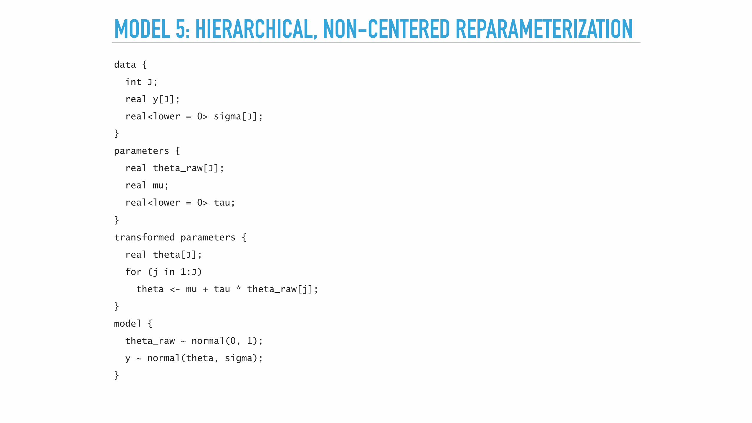
MODEL 5: HIERARCHICAL, NON-CENTERED REPARAMETERIZATIONdata {
int J;
real y[J];
real<lower = 0> sigma[J];
}
parameters {
real theta_raw[J];
real mu;
real<lower = 0> tau;
}
transformed parameters {
real theta[J];
for (j in 1:J)
theta <- mu + tau * theta_raw[j];
}
model {
theta_raw ~ normal(0, 1);
y ~ normal(theta, sigma);
}

MODEL 5: HIERARCHICAL, NON-CENTERED REPARAMETERIZATION> fit5
Inference for Stan model: eight_schools_5.
4 chains, each with iter=2000; warmup=1000; thin=1;
post-warmup draws per chain=1000, total post-warmup draws=4000.
mean se_mean sd 2.5% 25% 50% 75% 97.5% n_eff Rhat
theta_raw[1] 0.43 0.02 0.95 -1.56 -0.19 0.47 1.09 2.23 1988 1.00
theta_raw[2] 0.00 0.02 0.89 -1.84 -0.57 0.00 0.59 1.75 3048 1.00
theta_raw[3] -0.22 0.02 0.95 -2.01 -0.87 -0.23 0.42 1.64 3282 1.00
theta_raw[4] -0.03 0.02 0.86 -1.71 -0.60 -0.03 0.53 1.70 2909 1.00
theta_raw[5] -0.37 0.02 0.84 -1.98 -0.93 -0.38 0.18 1.33 2573 1.00
theta_raw[6] -0.23 0.02 0.87 -1.97 -0.79 -0.23 0.35 1.52 2823 1.00
theta_raw[7] 0.36 0.02 0.88 -1.53 -0.19 0.39 0.95 1.99 2945 1.00
theta_raw[8] 0.06 0.02 0.95 -1.82 -0.55 0.06 0.66 1.93 2659 1.00
mu 7.82 0.15 5.04 -2.25 4.72 7.72 11.02 17.54 1183 1.00
tau 6.68 0.18 5.38 0.28 2.69 5.49 9.25 19.99 928 1.00
theta[1] 11.70 0.27 8.73 -2.02 6.12 10.38 15.91 33.14 1020 1.00
theta[2] 7.96 0.11 6.28 -4.12 3.96 7.86 11.83 20.89 3092 1.00
theta[3] 5.89 0.16 7.86 -11.69 1.64 6.32 10.75 20.51 2519 1.00
theta[4] 7.53 0.13 6.46 -5.81 3.77 7.56 11.49 20.47 2622 1.00
theta[5] 4.89 0.12 6.14 -8.70 1.31 5.40 9.00 16.09 2766 1.00
theta[6] 5.99 0.12 6.62 -8.25 2.08 6.34 10.18 18.03 2943 1.00
theta[7] 10.70 0.14 6.78 -1.41 6.26 10.06 14.72 25.91 2374 1.00
theta[8] 8.34 0.18 8.00 -7.21 3.70 7.98 12.75 25.99 1961 1.00
lp__ -4.77 0.09 2.65 -10.77 -6.31 -4.44 -2.90 -0.40 972 1.01
Samples were drawn using NUTS(diag_e) at Wed Jun 1 01:47:53 2016.
TAKEAWAYS
▸ Easy to express hierarchical models in Stan!
▸ Discussed how to get around some divergent transitions
▸ Increase adapt_delta
▸ Non-centered reparameterization

FUNCTIONS

STAN FUNCTIONS IN R!
1. Write Stan program with a function.
2. In R:
cppcode <- stanc("functions.stan")
expose_stan_functions(cppcode)
OR
fit <- stanc("functions.stan")
expose_stan_functions(fit)

ACCESSING PARTS OF THE STAN PROGRAM IN R
▸ get_num_upars(fit)
▸ log_prob(fit, upars)
▸ grad_log_prob(fit, upars)
▸ constrain_pars(fit, upars)
▸ unconstrain_pars(fit, pars)


