Junos ® Networking Technologies Series It’s day one and you need to deploy IPv6. Where to start? This time-saving booklet and your Junos OS devices can get your network humming in no time. All on IPv6. By Chris Grundemann DAY ONE: EXPLORING IPV6
Transcript
Junos® Networking Technologies Series
It’s day one and you need to deploy IPv6.
Where to start? This time-saving booklet
and your Junos OS devices can get your
network humming in no time. All on IPv6.
By Chris Grundemann
DAY ONE: EXPLORING IPV6
Juniper Networks Day One books provide just the information you need to know on day one. That’s because they are written by subject matter experts who specialize in getting networks up and running. Visit www.juniper.net/dayone to peruse the complete library.
Published by Juniper Networks Books
DAY ONE: EXPLORING IPV6
The impending exhaustion of IPv4 addresses is prompting many network operators to
look closer at ways to provide more address space, including IPv6 and NAT solutions.
When deploying IPv6, you can gain a great advantage by using Juniper Networks high-end
routers because IPv6 has been implemented directly in the ASICs (Application-Specific
Integrated Circuit). Having IPv6 compatibility in the hardware means that IPv6 packets
can be forwarded at line rate – unlike many competing routers. Additionally, the Junos OS
makes configuring and troubleshooting an IPv6 network a snap. As you read this booklet
and work through the topics in your lab, you’ll progressively gain a fuller understanding of
IPv6 configuration and operation in Junos. The layered, methodical progression provided
will get you up to speed on this crucial networking technology quickly and easily.
IT’S DAY ONE AND YOU HAVE A JOB TO DO, SO LEARN HOW TO:
n Understand IPv6 address length, and read IPv6 addresses.
n Add family inet6 and IPv6 addresses to all types of interfaces.
n Set up and test IPv6 neighbor discovery and how to implement static routes in IPv6.
n Use basic IPv6 troubleshooting and verification commands, such as ping, traceroute, and various show commands.
n Understand how the three IGPs support IPv6: RIPng, OSPF3, and IS-IS.
“Chris Grundemann has created a fantastic introduction to IPv6 that covers the protocol struc-
ture as well as Junos implementation details. This guide is easy to follow and is an easy-to-digest
tutorial on getting your feet wet in IPv6. This is a great addition to the other Day One booklets
that Juniper has made available to everyone.”
Scott Hogg, Director of Advanced Technology Services, GTRI,
Juniper Networks assumes no responsibility for any inaccuracies in this document. Juniper Networks reserves the right to change, modify, transfer, or otherwise revise this publication without notice. Products made or sold by Juniper Networks or components thereof might be covered by one or more of the following patents that are owned by or licensed to Juniper Networks: U.S. Patent Nos. 5,473,599, 5,905,725, 5,909,440, 6,192,051, 6,333,650, 6,359,479, 6,406,312, 6,429,706, 6,459,579, 6,493,347, 6,538,518, 6,538,899, 6,552,918, 6,567,902, 6,578,186, and 6,590,785.
Published by Juniper Networks BooksWriter: Chris GrundemannEditor in Chief: Patrick AmesCopyediting and Proofing: Nancy KoerbelJunos Program Manager: Cathy Gadecki
ISBN: 978-1-936779-06-2 (print)Printed in the USA by Vervante Corporation.ISBN: 978-1-936779-07-9 (ebook)
Version History: v3 January 2011 4 5 6 7 8 9 10 #7100132-en
About the AuthorChris Grundemann specializes in the design, implementa-tion, and operation of large IP, Ethernet and Wireless Ethernet networks. He is JNCIE-M #449 and is currently engaged with tw telecom inc., where he is responsible for leading technology efforts toward the evaluation, design, implementation, and maintenance of existing and next-generation technologies.
Chris is the founding Chair of CO ISOC, the Colorado chapter of the Internet Society, and an active participant in the ARIN policy process. He is the lead developer and chief editor for Burning With The Bush, a Juniper Networks focused news and information site, and also maintains a personal weblog aimed towards Internet related posts typically focusing on network operations, tech-policy, and the future of the Internet.
Author’s AcknowledgmentsThe author would like to thank everyone who contrib-uted to the creation of this book. Friend and Juniper resident engineer Nate Day sparked the inspiration to write for Juniper Networks in the first place. Patrick Ames was absolutely crucial as both editor and instructor. Cathy Gadecki got the project off the ground and added great insight to the review process. Becca Nitzan lent her exceptional technical expertise through-out. Mathew Moriarty knows what he did. Ryan Privette and Mark Calkins help to keep me motivated by consistently being great engineers and making me want to be better myself. The IETF and all of its contributors created the open technical standards that define and drive the IPv6 protocol, without which this book (and possibly the future of the Internet) would not exist. Most importantly I would like to thank my wife, Erin Grundemann, for giving me the time, support and love that it takes to do all of the things I do, including writing this book. Thank you all.
This book is available in a variety of formats at: www.juniper.net/dayone. Send your suggestions, comments, and critiques by email to [email protected]. Follow the Day One series on Twitter: @Day1Junos
ii
iii
Dedicated to Paul L. Grundemann, 1949 – 2010
A greater father no one could ask for, and a greater man the world has not often seen. Thanks for everything, Dad.
iv
Welcome to Day One
Day One: Exploring IPv6 is the first booklet in the Junos Networking Technologies series of Day One booklets. This series is intended to guide the reader progressively through a variety of key networking technologies, including the IPv6 protocol as implemented in Junos.
This first booklet focuses on native IPv6 functionality. Although it is extremely likely that you will be implementing IPv6 alongside IPv4 in any network, a progressive, IPv6-native-first approach grants a much better overall understanding of IPv6 than jumping right into integra-tion would. Why?
The first reason is that IPv6 is a new and separate protocol from IPv4, despite the many similarities one might find in configuration and operation between the two protocols, especially when implementing them in Junos. In fact, IPv6 and IPv4 packets are not compatible on the wire. Put simply, when implementing IPv6 you are layering a new logical network onto your existing physical topology. The Day One booklets in this series will approach IPv6 from this perspective.
The other reason for starting only with IPv6 and working up to protocol integration in later booklets is a practical one. As you read these booklets and work through the topics in your lab, you’ll progres-sively gain a fuller understanding of IPv6 configuration and operation in Junos. This layered, methodical progression will help you get up to speed without missing anything important.
What You Need to Know Before Reading this Book
You will need a basic understanding of Junos and the Junos CLI, including configuration changes using edit mode.
You should have at least some experience with IPv4 networks including basic routing knowledge.
This booklet assumes that you have the ability to configure basic IPv4 connectivity, including interface addressing and static routes, and to troubleshoot a basic network as needed.
Knowledge of IPv4 routing protocols such as RIP, OSPF and IS-IS is helpful as well.
This booklet is written for engineers with experience in either Enterprise or Service Provider networks.
This booklet is written primarily for first-time users of IPv6 or first time users of IPv6 in Junos, but is written in such a way that it will also serve as a refresher for experienced users.
After Reading this Book, You’ll be Able to
Understand IPv6 address length, read IPv6 addresses, and under-stand IPv6 classifications and how to recognize various well known IPv6 addresses.
Enable IPv6 on your network by adding family inet6 and IPv6 addresses to all types of interfaces.
Set up and test IPv6 neighbor discovery, and implement static routes in IPv6.
Use basic IPv6 troubleshooting and verification commands, such as ping, traceroute, and various show commands.
Complete all of the configuration and testing tasks required to build a basic IPv6 native network.
Understand how the three Interior Gateway Protocols (IGPs) support IPv6: RIPng, OSPF3, and IS-IS.
Enable and verify the operation of basic dynamic IPv6 routing within your network using your choice of IGP.
v
Supplemental Appendix
If you’re reading the print edition of this book, Day One: Exploring IPv6, it is alternatively available in a PDF version and a eBook edition, both of which include a few supplemental pages as an appendix. Go to www.juniper.net/dayone and download the free PDF or eBook of this book and examine the other titles and information available from Juniper Networks.
NOTE We’d like to hear your comments and critiques. Please send us your suggestions by email at [email protected].
Answers to the Try It Yourself Questions . . . . . . . . 24
8 Day One: Exploring IPv6
If you are reading this booklet, you are probably looking to build your understanding of IPv6 (Internet Protocol version 6) and how it may work in your network. The impending exhaustion of IPv4 (Internet Protocol version 4) addresses is prompting many network operators to take a closer look at the possible solutions, including IPv6 and various forms of Network Address Translation (NAT).
There are roughly 4.2 billion addresses available in IPv4. Yet, with many users requiring more than one IP address per person for a variety of personal devices and other addressing uses (including networking equip-ment and interfaces, subnetting, etc.) the available IPv4 address pool is insufficient to meet future needs.
A quick comparison of global addressing requirements and the currently available pool of addresses, makes it very evident that the existing IPv4 approach will simply not scale with the global Internet and its multitude of attached networks and devices. The current projection shows that the IPv4 free pool at IANA will exhaust in first half of 2011 and the RIRs will exhaust their supply shortly after. IPv6 is a long term solution to this scaling problem as it offers a theoretical maximum of 3.4x10^38 address-es. That is...
Although IPv4 address ‘exhaustion’ may sound frightening, the first thing to keep in mind is that the use of NAT solutions will serve to bridge between the current IPv4-based content/endpoints and new IPv6 solu-tions. Thus, IPv4 address exhaustion is not the end of the Internet—not nearly.
IPv6 and IPv4 Compatibility
If you are new to IPv6, you may have questions about the compatibility between IPv6 and IPv4. The IPv4 and IPv6 protocols are not interoperable on the wire, creating additional considerations. For example, if you are an operator, assigning new IPv6 addresses won’t solve your subscribers’ needs for reaching IPv4 only endpoints.
Chapter 1: Introducing IPv6 9
If you are running out of IPv4 addresses, you need a transition mech-anism. Adopting a form of NAT technology enables you to support the immediate IPv4 addressing needs of your subscribers/users. All NAT solutions revolve around the notion of sharing existing pools of IPv4 addresses. For broadband service, it means sharing one IPv4 address among many subscribers. For commercial service, it means offering much smaller blocks of IPv4 addresses to be shared within the enter-prise network. There are various flavors of those NAT technologies: DS-Lite, NAT444, NAT64, etc.
Those techniques will help you maintain an IPv4 service while the move to IPv6 happens. To prepare for it the first steps are to learn more about IPv6 and get your network IPv6 ready.
MORE Find out more about the issues of IPv4 address depletion and potential solutions in the Juniper whitepaper: Tools and Strategies for Coping with IPv4 Address Depletion. The paper provides a frank analysis of the current situation and the available technologies for an IPv4 address exhausted world.
With the first step of learning more about IPv6 in mind, this chapter takes a quick, vender-agnostic look at the IPv6 protocol, from address length to packet format. Along the way it details a lot more. It’s intend-ed to be a solid foundation from which to build the IPv6 configuration and operation knowledge required in subsequent chapters.
Understanding IPv6 Addresses
The first thing you notice about IPv6 is that the addresses look quite different from IPv4 addresses.
The primary difference, of course, is length. IPv4 addresses are 32 bits long and IPv6 addresses are 128 bits long. This means that an IPv4 address is made up of thirty-two 1s and 0s while an IPv6 address is made up of 128 of them – 128 binary digits. This massive length forces IPv6 addresses to be written using a different notation than IPv4 addresses, and thus makes them very easy to distinguish from IPv4 addresses.
10 Day One: Exploring IPv6
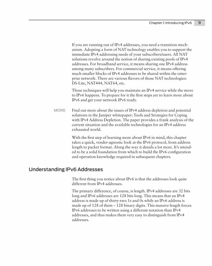
This length and new notation can make it harder to initially understand IPv6 addresses, however, if only because of their novelty. Figure 1.1 shows what a 128-bit IPv6 address in binary notation looks like, the way it would be written inside of an IPv6 packet.
If you were to use the dotted-decimal notation familiar to us from IPv4, 192.0.2.1, for example, you would need to break this 128-bit address into sixteen 8-bit sections, and the resulting address would look something like this: 32.1.13.184.0.0.0.0.0.0.0.0.0.0.0.1. This is a little unwieldy, to say the least!
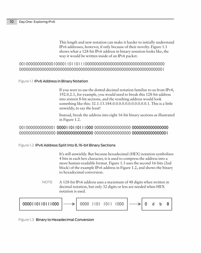
Instead, break the address into eight 16-bit binary sections as illustrated in Figure 1.2.
Figure 1.2 IPv6 Address Split Into 8, 16-bit Binary Sections
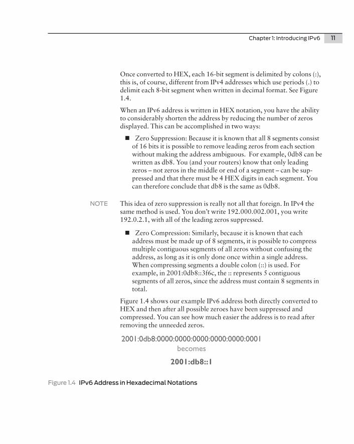
It’s still unwieldy. But because hexadecimal (HEX) notation symbolizes 4 bits in each hex character, it is used to compress the address into a more human-readable format. Figure 1.3 uses the second 16-bits (2nd block) of the example IPv6 address in Figure 1.2, and shows the binary to hexadecimal conversion.
NOTE A 128-bit IPv6 address uses a maximum of 48 digits when written in decimal notation, but only 32 digits or less are needed when HEX notation is used.
0000110110111000 0000 1101 1011 1000 0 d b 8
Figure 1.3 Binary to Hexadecimal Conversion
10
Chapter 1: Introducing IPv6 11
Once converted to HEX, each 16-bit segment is delimited by colons (:), this is, of course, different from IPv4 addresses which use periods (.) to delimit each 8-bit segment when written in decimal format. See Figure 1.4.
When an IPv6 address is written in HEX notation, you have the ability to considerably shorten the address by reducing the number of zeros displayed. This can be accomplished in two ways:
nZero Suppression: Because it is known that all 8 segments consist of 16 bits it is possible to remove leading zeros from each section without making the address ambiguous. For example, 0db8 can be written as db8. You (and your routers) know that only leading zeros – not zeros in the middle or end of a segment – can be sup-pressed and that there must be 4 HEX digits in each segment. You can therefore conclude that db8 is the same as 0db8.
NOTE This idea of zero suppression is really not all that foreign. In IPv4 the same method is used. You don’t write 192.000.002.001, you write 192.0.2.1, with all of the leading zeros suppressed.
nZero Compression: Similarly, because it is known that each address must be made up of 8 segments, it is possible to compress multiple contiguous segments of all zeros without confusing the address, as long as it is only done once within a single address. When compressing segments a double colon (::) is used. For example, in 2001:0db8::3f6c, the :: represents 5 contiguous segments of all zeros, since the address must contain 8 segments in total.
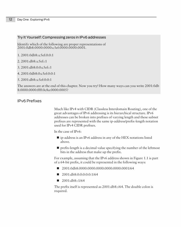
Figure 1.4 shows our example IPv6 address both directly converted to HEX and then after all possible zeroes have been suppressed and compressed. You can see how much easier the address is to read after removing the unneeded zeros.
2001:0db8:0000:0000:0000:0000:0000:0001becomes
2001:db8::1
Figure 1.4 IPv6 Address in Hexadecimal Notations
12 Day One: Exploring IPv6
Try It Yourself: Compressing zeros in IPv6 addresses Identify which of the following are proper representations of 2001:0db8:0000:0000:c5ef:0000:0000:0001.
1. 2001:0db8::c5ef:0:0:1
2. 2001:db8::c5ef::1
3. 2001:db8:0:0:c5ef::1
4. 2001:0db8:0:c5ef:0:0:1
5. 2001:db8::c5ef:0:0:1
The answers are at the end of this chapter. Now you try! How many ways can you write 2001:0db8:0000:0000:ffff:0c8a:0000:0005?
IPv6 Prefixes
Much like IPv4 with CIDR (Classless Interdomain Routing), one of the great advantages of IPv6 addressing is its hierarchical structure. IPv6 addresses can be broken into prefixes of varying length and these subnet prefixes are represented with the same ip-address/prefix-length notation used for IPv4 CIDR prefixes.
In the case of IPv6:
nip-address is an IPv6 address in any of the HEX notations listed above.
nprefix-length is a decimal value specifying the number of the leftmost bits in the address that make up the prefix.
For example, assuming that the IPv6 address shown in Figure 1.1 is part of a 64-bit prefix, it could be represented in the following ways:
n2001:0db8:0000:0000:0000:0000:0000:0001/64
n2001:db8:0:0:0:0:0:1/64
n2001:db8::1/64
The prefix itself is represented as 2001:db8::/64. The double colon is required.
Chapter 1: Introducing IPv6 13
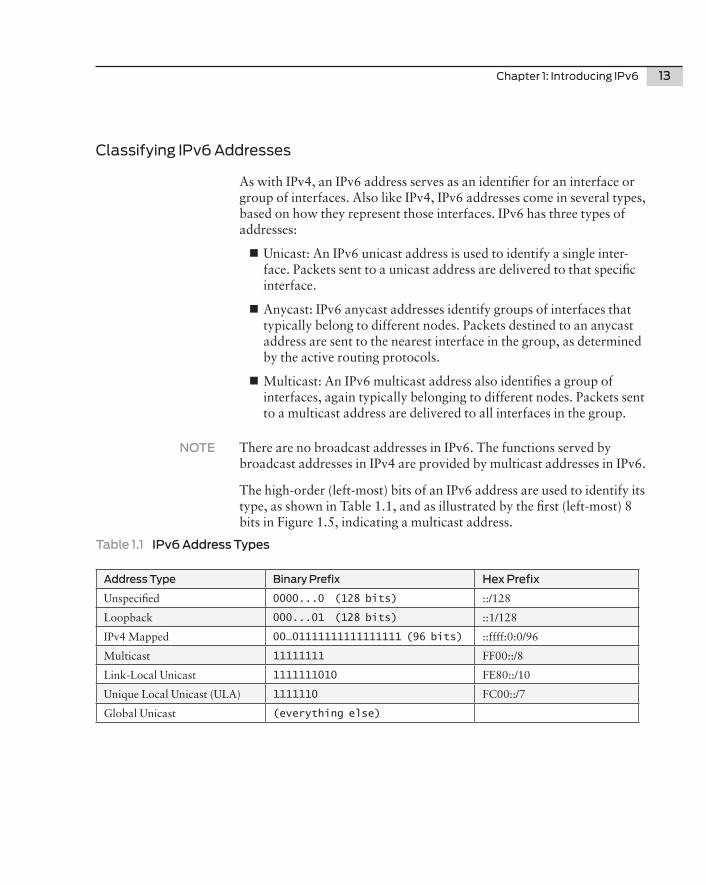
Classifying IPv6 Addresses
As with IPv4, an IPv6 address serves as an identifier for an interface or group of interfaces. Also like IPv4, IPv6 addresses come in several types, based on how they represent those interfaces. IPv6 has three types of addresses:
nUnicast: An IPv6 unicast address is used to identify a single inter-face. Packets sent to a unicast address are delivered to that specific interface.
nAnycast: IPv6 anycast addresses identify groups of interfaces that typically belong to different nodes. Packets destined to an anycast address are sent to the nearest interface in the group, as determined by the active routing protocols.
nMulticast: An IPv6 multicast address also identifies a group of interfaces, again typically belonging to different nodes. Packets sent to a multicast address are delivered to all interfaces in the group.
NOTE There are no broadcast addresses in IPv6. The functions served by broadcast addresses in IPv4 are provided by multicast addresses in IPv6.
The high-order (left-most) bits of an IPv6 address are used to identify its type, as shown in Table 1.1, and as illustrated by the first (left-most) 8 bits in Figure 1.5, indicating a multicast address.
Anycast addresses are taken from the global unicast pool. Anycast and unicast addresses can not be distinguished based on format.
Multicast Addresses
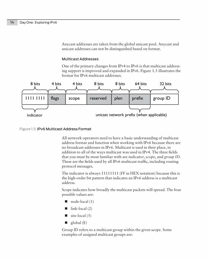
One of the primary changes from IPv4 to IPv6 is that multicast address-ing support is improved and expanded in IPv6. Figure 1.5 illustrates the format for IPv6 multicast addresses.
reserved 1111 1111 prefix
8 bits
flags scope plen
group ID
4 bits
4 bits
8 bits
8 bits
64 bits
32 bits
indicator
unicast network prefix (when applicable)
Figure 1.5 IPv6 Multicast Address Format
All network operators need to have a basic understanding of multicast address format and function when working with IPv6 because there are no broadcast addresses in IPv6. Multicast is used in their place, in addition to all of the ways multicast was used in IPv4. The three fields that you must be most familiar with are indicator, scope, and group ID. These are the fields used by all IPv6 multicast traffic, including routing protocol messages.
The indicator is always 11111111 (FF in HEX notation) because this is the high-order bit pattern that indicates an IPv6 address is a multicast address.
Scope indicates how broadly the multicast packets will spread. The four possible values are:
nnode-local (1)
nlink-local (2)
nsite-local (5)
nglobal (E)
Group ID refers to a multicast group within the given scope. Some examples of assigned multicast groups are:
Chapter 1: Introducing IPv6 15
nall nodes (1) – valid scope of 1 or 2.
nall-routers (2) – valid scopes are 1, 2, or 5.
nOSPF Designated Routers (6) – only valid with scope of 2.
nNTP (101) – valid in any scope.
Try It Yourself: Identifying Multicast Addresses
Follow along and test yourself with these examples of multicast addresses:
1. FF02::1
2. FF02::6
3. FF05::101
The answers are at the end of this chapter.
MORE? To learn more about IPv6 multicast addresses, see RFC 2375 “IPv6 Multicast Address Assignments,” RFC 3306 “Unicast-Prefix-based IPv6 Multicast Addresses,” and, RFC 3307 “Allocation Guidelines for IPv6 Multicast Addresses.”
Global Unicast Addresses
As with IPv4, unicast addresses are the most common type of IPv6 address you will work with. Because of the abundance of addresses available with IPv6, it is very likely that virtually every machine attached to your network has at least one global unicast address assigned to each interface. (Read that sentence again, if you don’t mind.)
Because of this, all IPv6 address space not currently specified for another purpose is reserved for use as global unicast addresses. Only a single /3 is currently allocated for use, however. The IETF (Internet Engineering Task Force) has assigned binary prefix 001 (HEX prefix 2000::/3) to IANA (Internet Assigned Numbers Authority) for use on the Internet. This means that for now, all valid global unicast addresses begin with the 2000::/3 prefix.
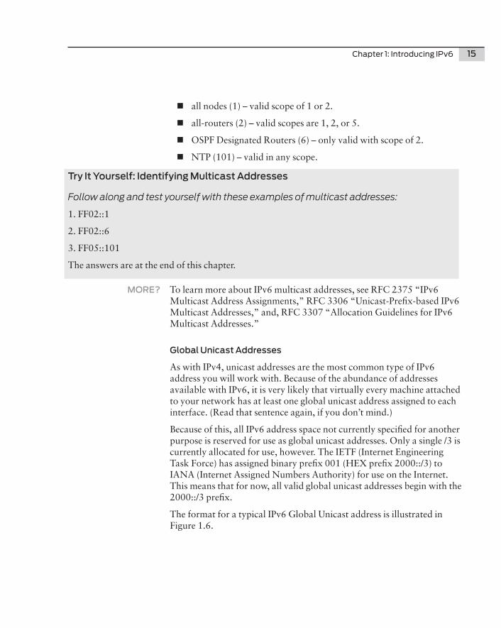
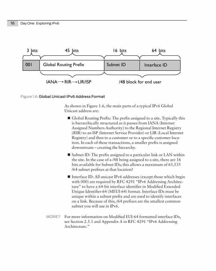
The format for a typical IPv6 Global Unicast address is illustrated in Figure 1.6.
16 Day One: Exploring IPv6
Subnet ID Global Routing Prefix
64 bits
/48 block for end user
Interface ID
45 bits
16 bits
IANA RIR LIR/ISP
001
3 bits
Figure 1.6 Global Unicast IPv6 Address Format
As shown in Figure 1.6, the main parts of a typical IPv6 Global Unicast address are:
nGlobal Routing Prefix: The prefix assigned to a site. Typically this is hierarchically structured as it passes from IANA (Internet Assigned Numbers Authority) to the Regional Internet Registry (RIR) to an ISP (Internet Service Provider) or LIR (Local Internet Registry) and then to a customer or to a specific customer loca-tion. In each of these transactions, a smaller prefix is assigned downstream – creating the hierarchy.
nSubnet ID: The prefix assigned to a particular link or LAN within the site. In the case of a /48 being assigned to a site, there are 16 bits available for Subnet IDs; this allows a maximum of 65,535 /64 subnet prefixes at that location!
nInterface ID: All unicast IPv6 addresses (except those which begin with 000) are required by RFC 4291 “IPv6 Addressing Architec-ture” to have a 64-bit interface identifier in Modified Extended Unique Identifier-64 (MEUI-64) format. Interface IDs must be unique within a subnet prefix and are used to identify interfaces on a link. Because of this, /64 prefixes are the smallest common subnet you will use in IPv6.
MORE? For more information on Modified EUI-64 formatted interface IDs, see Section 2.5.1 and Appendix A in RFC 4291 “IPv6 Addressing Architecture.”
Chapter 1: Introducing IPv6 17
Introducing Special IPv6 Addresses
If you re-examine Table 1.1, you can see there are several special addresses and address groups within IPv6. Some of these might be familiar to you from your work with IPv4 addressing, and some are new in IPv6:
nUnspecified address (::/128): This all-zeros address refers to the host when the host does not know its own address. The unspecified address is typically used in the source field by a device seeking to have its IPv6 address assigned.
nLoopback address (::1/128): IPv6 has a single address for the loopback function, instead of a whole block as in IPv4.
nIPv4-Mapped addresses (::ffff:0:0/96): A /96 prefix leaves 32 bits, exactly enough to hold an embedded IPv4 address. IPv4-Mapped IPv6 addresses are used to represent an IPv4 node’s address as an IPv6 address. This address type was defined to help with the transition from IPv4 to IPv6.
MORE? For more background on IPv4-mapped IPv6 addresses, see RFC 4038 “Application Aspects of IPv6 Transition.” Also, be aware that there may be security risks associated with using IPv4-mapped addresses. See the IETF draft “IPv4-Mapped Addresses on the Wire Considered Harmful” for more information.
nLink-Local unicast addresses (FE80::/10): As the name implies, Link-Local addresses are unicast addresses to be used on a single link. Packets with a Link-Local source or destination address will not be forwarded to other links. These addresses are used for neighbor discovery, automatic address configuration, and in circumstances when no routers are present.
nUnique local unicast addresses (FC00::/7): Commonly known as ULA, this group of addresses is for local use, within a site or group of sites. Although globally unique, these addresses are not routable on the global Internet. This author looks at ULA as a kind of upgraded RFC 1918 (private) address space for IPv6.
MORE? For more information on ULA, read RFC 4193 “Unique Local IPv6 Unicast Addresses.”
18 Day One: Exploring IPv6
Understanding the IPv6 Protocol
By now you should have a firm grasp on the format and types of IPv6 addresses so it’s time to dig into the IPv6 protocol and examine IPv6’s multiple header structure, neighbor discovery, and SLAAC. We’ll also take a quick look at just how many IPv6 addresses there really are.
IPv6 Headers
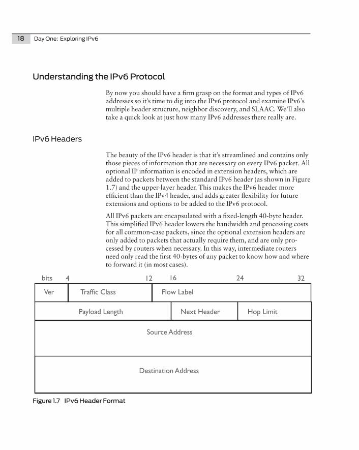
The beauty of the IPv6 header is that it’s streamlined and contains only those pieces of information that are necessary on every IPv6 packet. All optional IP information is encoded in extension headers, which are added to packets between the standard IPv6 header (as shown in Figure 1.7) and the upper-layer header. This makes the IPv6 header more efficient than the IPv4 header, and adds greater flexibility for future extensions and options to be added to the IPv6 protocol.
All IPv6 packets are encapsulated with a fixed-length 40-byte header. This simplified IPv6 header lowers the bandwidth and processing costs for all common-case packets, since the optional extension headers are only added to packets that actually require them, and are only pro-cessed by routers when necessary. In this way, intermediate routers need only read the first 40-bytes of any packet to know how and where to forward it (in most cases).
bits 4 12 16 24 32
Source Address
Hop Limit
Flow Label
Payload Length
Traffic Class
Next Header
Ver
Destination Address
Figure 1.7 IPv6 Header Format
Chapter 1: Introducing IPv6 19
These components make up the IPv6 header, shown in Figure 1.7:
nVersion: 4-bit IP version number, set to 6 for IPv6 packets.
nTraffic Class: The traffic class field is 8 bits long and is used to mark packets for differentiated service similar to the IPv4 Type of Service and Precedence bits. This practice is commonly called Class of Service (CoS) or Quality of Service (QoS) depending on the imple-mentation.
nFlow Label: This 20-bit field is still experimental but its intent is to label sequences of packets (flows) that require special handling. RFC 2460 “IPv6 Specification” suggests non-default quality of service and real-time service as example uses for the flow label.
nPayload Length: Unlike IPv4, which lists the total packet length in its header, the IPv6 header specifies payload length – in other words, the length of everything that follows this header in the packet – in-cluding any extension headers as well as the data being carried. This field is 16 bits long.
nNext Header: An 8-bit selector which uses the same values as the IPv4 protocol field to identify the type of header that immediately follows the IPv6 header.
nHop Limit: Like Time To Live (TTL) in the IPv4 header, this 8-bit integer is decremented by 1 each time the packet is forwarded. If the Hop Limit reaches 0, the packet is discarded.
nSource Address: The 128-bit IPv6 address of the node sending this packet.
nDestination Address: The 128-bit IPv6 address of the node intended to receive this packet.
In addition to the required IPv6 header, IPv6 packets may have one or more of the optional extension headers.
MORE? To learn more about the IPv6 header (and extension headers), see RFC 2460 “Internet Protocol, Version 6 (IPv6) Specification.”
Extension Headers
Because IPv6 carries optional information in extension headers and not in the IPv6 header itself, there is always the possibility to add new functionality to IPv6 by introducing new extension headers.
20 Day One: Exploring IPv6
There are currently six extension headers defined in IPv6:
nHop-by-Hop Options: The Hop-by-Hop Options header is used to carry information that must be examined by all routers along the packet’s path.
nDestination Options: Just as the name implies, this header carries information that is meant for the packet’s destination node(s).
nRouting: The IPv6 Routing header provides similar functionality to the Loose Source and Record Route options in IPv4. It specifies one or more intermediate nodes that must be included in the packet’s path from source to destination.
nFragment: Packet fragmentation is rare in IPv6 because nodes use Path MTU Discovery to determine the MTU (Maximum Trans-mission Unit) allowed between any two points. When an applica-tion is unable to adjust its packet size appropriately, the source node can use the Fragment header to fragment the packet for reassembly at the destination. Unlike IPv4, IPv6 packets can only be fragmented by the originating node.
nAuthentication: The Authentication header (AH) is a part of IPSec and provides connectionless integrity, data origin authentication, and anti-replay protection. See RFC 4302 “IP Authentication Header” for all the details.
nEncapsulating Security Payload: Like the Authentication header, the Encapsulating Security Payload (ESP) header is part of the IPSec suite. This header is used to provide integrity, authentica-tion, confidentiality, and an anti-replay service. See RFC 4303 “IP Encapsulating Security Payload (ESP)” for more information.
MORE? For more information on how the AH and ESP headers work together and the security services they provide, see RFC 4301 “Security Archi-tecture for the Internet Protocol.”
Neighbor Discovery and SLAAC
IPv6 Neighbor Discovery combines and improves upon the functional-ity found in Address Resolution Protocol (ARP), Internet Control Message Protocol (ICMP), Router Discovery, and ICMP-Redirects in IPv4, and adds some new features as well.
Chapter 1: Introducing IPv6 21
IPv6 Neighbor Discovery includes four main functions:
nRouter Discovery: Routers periodically send out router advertise-ment messages to announce their presence, advertise prefixes that are on-link, assist in address configuration, and share other infor-mation about the link (MTU, hop limit, etc.)
nNeighbor Discovery: IPv6 nodes communicate their link-layer addresses to each other using neighbor solicitation and neighbor advertisement messages. These messages are also used to detect duplicate addresses and test reachability.
nNeighbor Unreachability Detection: IPv6 nodes rely on positive confirmation of packet delivery. This is accomplished in two ways. First, nodes “listen” for new acknowledgements being returned, or for similar upper-layer protocol confirmation that packets sent to a neighbor are in fact reaching their destination. When such confir-mation is absent, the node sends unicast neighbor solicitation messages to confirm next-hop reachability.
nRedirects: Very similar to the ICMPv4 Redirect feature, the IC-MPv6 Redirect message is used by routers to inform on-link hosts of a better next-hop for a given destination. The intent is to allow the router(s) to help hosts make the most efficient local routing decisions possible.
As mentioned prevously, Neighbor Discovery has many improvements and new features when compared to the corresponding IPv4 protocols. For instance, Neighbor Discovery moves address resolution to the ICMP layer, which makes it much less media dependent than ARP as well as adding the ability to use IP layer security when needed.
Additionally, Neighbor Discovery uses link-local addresses. This allows all nodes to maintain their router associations even when the site is renumbered to a new global prefix.
Another improvement worth noting is that Neighbor Discovery messages carry link-layer address information so a single message (or pair of messages) is all that is needed for nodes to resolve the others’ addresses; no additional address resolution is needed.
Neighbor Unreachability Detection is built in, making packet delivery much more robust in a changing network. Using Neighbor Unreach-ability Detection, Neighbor Discovery will detect router failures, link failures, and most notably partial link failures such as one-way commu-nication.
22 Day One: Exploring IPv6
And finally, IPv6 Router Advertisements carry prefixes (including netmasks) and support multiple prefixes on the same link. Hosts can learn on-link prefixes from router advertisements or, when the router is configured to withhold them, from redirects as needed.
SLAAC
In addition to all the other improvements it brings to the networking world, Neighbor Discovery also enables address autoconfiguration – namely Stateless Address Autoconfiguration (SLAAC). IPv6 main-tains the capability for stateful address assignment through DHCPv6 (and static assignment), but SLAAC provides a lightweight address configuration method that may be desirable in many circumstances.
SLAAC provides plug-and-play IP connectivity in two phases: Phase 1: Link-Local address assignment; and then, in Phase 2: Global address assignment.
Phase 1 - Link-Local Address
Here are the Phase 1 steps for local connectivity:
1. Link-Local Address Generation: Any time that a multicast-capable IPv6-enabled interface is turned up, the node generates a link-local address for that interface. This is done by appending an interface identifier to the link-local prefix (FE80::/10).
2. Duplicate Detection: Before assigning the new link-local address to its interface, the node verifies that the address is unique. This is accomplished by sending a Neighbor Solicitation message destined to the new address. If there is a reply, then the address is a dupli-cate and the process stops, requiring operator intervention.
3. Link-Local Address Assignment: If the address is unique, the node assigns it to the interface it was generated for.
At this point, the node has IPv6 connectivity to all other nodes on the same link. Phase 2 can only be completed by hosts; the router’s interface addresses must be configured by other means.
Phase 2 - Global Address
And Phase 2 steps for global connectivity:
1. Router Advertisement: The node sends a Router Solicitation to prompt all on-link routers to send it router advertisements. When
Chapter 1: Introducing IPv6 23
the router is enabled to provide stateless autoconfiguration support, the router advertisement will contain a subnet prefix for use by neighboring hosts.
2. Global Address Generation: Once it receives a subnet prefix from a router, the host generates a global address by appending the interface id to the supplied prefix.
3. Duplicate Address Detection: The host again performsDuplicate Address Detection (DAD), this time for the new global address.
4. Global Address Assignment: Assuming that the address is not a duplicate, the host assigns it to the interface.
There you have it, full IPv6 global connectivity with no manual host configuration and very little router configuration.
MORE? Want to learn more about Neighbor Discovery and SLAAC? Read RFC 4861 “Neighbor Discovery for IP version 6 (IPv6),” RFC 4862 “IPv6 Stateless Address Autoconfiguration,” and RFC 4339 “IPv6 Host Configuration of DNS Server Information Approaches.”
Counting IPv6 Addresses
When discussions about the number of IPv6 addresses arise, terms like unlimited and infinite are often bandied about, so let’s examine just how large the IPv6 address space is.
As noted previously, IPv6 addresses are made up of 128 bits, which yields a theoretical maximum of 3.4x10^38 addresses. The problem is that this is such a large number that it’s very difficult to get a solid grasp on what it actually means.
The common comparisons are that there are 5×10^28 (roughly 50,000,000,000,000,000,000,000,000,000) addresses per human on Earth or 2^96 (7.92281625 × 10^28) times more unique addresses than are available with IPv4. But this is not a fair comparison because the IPv6 standards are designed in such a way that individual IPv6 addresses are far less meaningful than individual IPv4 addresses.So let’s look at the number of IPv6 addresses not individually, but in meaningful blocks.
In a single IPv6 /32 there are 65,536 possible /48s. Since an IPv6 /48 is the “normal maximum” assignment you might rationally compare this to an IPv4 /24. To have 65,536 IPv4 /24s at your disposal you would need a /8 assigned to your organization. There are only 256 unique
24 Day One: Exploring IPv6
IPv4 /8s possible while there are about 4.2 billion IPv6 /32s. The difference is a factor of 16,777,216, a far cry from the 7.9 × 10^28 we get when comparing individual addresses.
This method does have its own problems though. An IPv6 /48 contains roughly a septillion (1.209 x 10^24) individual addresses while an IPv4 /24 holds only 256. Of course it is highly unlikely that anyone will ever add a septillion (or anything close to that) hosts to a single network, IPv6 or not (unless sometime in the future each planet or star system were its own unified network).
The bottom line is that you need to use IP addresses as efficiently as possible, whether they are version 6 or version 4.
Answers to the Try It Yourself Sections of Chapter 1
Try It Yourself: Compressing zeros in IPv6 addresses Identify which of the following are proper representations of 2001:0db8:0000:0000:c5ef:0000:0000:0001.
1. 2001:0db8::c5ef:0:0:1
2. 2001:db8::c5ef::1
3. 2001:db8:0:0:c5ef::1
4. 2001:0db8:0:c5ef:0:0:1
5. 2001:db8::c5ef:0:0:1
Try It Yourself: Identifying Multicast Addresses Follow along and test yourself with these examples of multicast ad-dresses:
1. FF02::1
All nodes on the same link as the sender, this address replaces the broad-cast function in IPv4.
One of the great advantages of using Juniper Networks high-end routers when building an IPv6 network is that IPv6 has been implemented directly in the ASICs (Application-Specific Integrated Circuit). Having IPv6 compatibility in the hardware means that IPv6 packets can be forwarded at line rate – unlike many competing routers. Additionally, the Junos OS makes configuring and troubleshooting an IPv6 network a snap.
After reading this chapter you will be able to complete all of the configu-ration and testing tasks required to build a basic IPv6 native network. You will learn how to assign IPv6 addresses to interfaces, how to set up and test IPv6 neighbor discovery, and how to implement static routes in IPv6. This chapter also introduces some IPv6 troubleshooting and verification commands, such as ping, traceroute and various show commands.
ALERT! Before tackling the tasks in this chapter, you really should have enough experience with the Junos CLI to maneuver unhindered in both opera-tional and configuration modes.
MORE? If you need more information on the Junos CLI, complete with some step-by-step instruction, see the Day One guide: Exploring the Junos CLI available at www.juniper.net/dayone.
IPv6 Test Bed
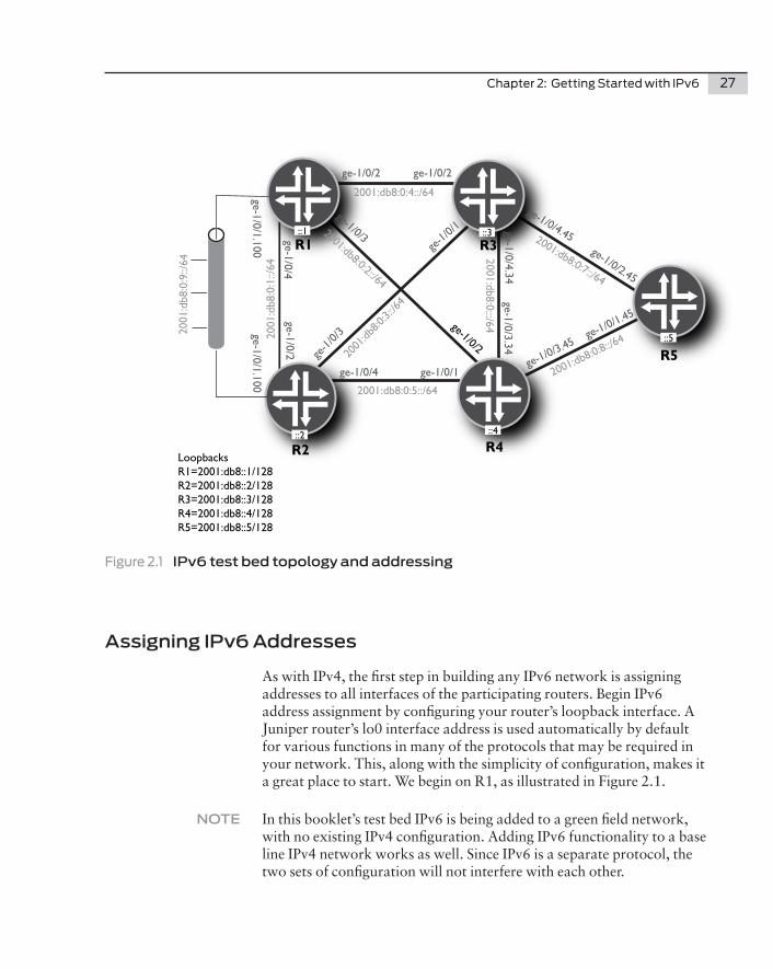
If you have access to a set of devices in a lab or other nonoperational environment, follow along with the examples in this booklet while exploring IPv6 and Junos. All of the examples on these pages, along with the Try It Yourself segments, are taken directly from the network illus-trated in Figure 2.1.
Chapter 2: Getting Started with IPv6 27
Figure 2.1 IPv6 test bed topology and addressing
Assigning IPv6 Addresses
As with IPv4, the first step in building any IPv6 network is assigning addresses to all interfaces of the participating routers. Begin IPv6 address assignment by configuring your router’s loopback interface. A Juniper router’s lo0 interface address is used automatically by default for various functions in many of the protocols that may be required in your network. This, along with the simplicity of configuration, makes it a great place to start. We begin on R1, as illustrated in Figure 2.1.
NOTE In this booklet’s test bed IPv6 is being added to a green field network, with no existing IPv4 configuration. Adding IPv6 functionality to a base line IPv4 network works as well. Since IPv6 is a separate protocol, the two sets of configuration will not interfere with each other.
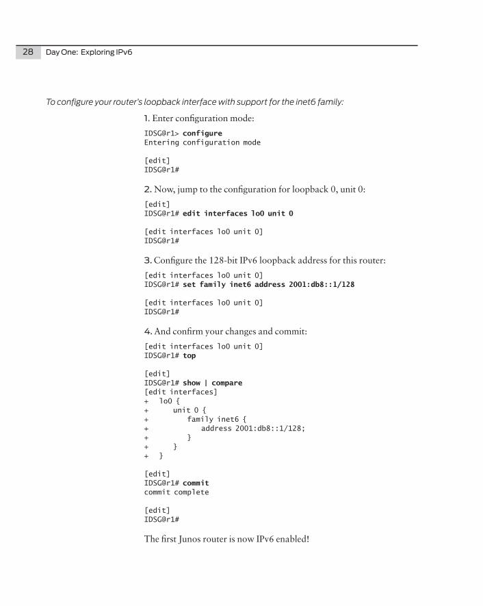
To configure your router’s loopback interface with support for the inet6 family:
1. Enter configuration mode:
IDSG@r1> configure Entering configuration mode
[edit]IDSG@r1#
2. Now, jump to the configuration for loopback 0, unit 0:
[edit]IDSG@r1# edit interfaces lo0 unit 0
[edit interfaces lo0 unit 0]IDSG@r1#
3. Configure the 128-bit IPv6 loopback address for this router:
[edit interfaces lo0 unit 0]IDSG@r1# set family inet6 address 2001:db8::1/128
[edit interfaces lo0 unit 0]IDSG@r1#
4. And confirm your changes and commit:
[edit interfaces lo0 unit 0]IDSG@r1# top
[edit]IDSG@r1# show | compare [edit interfaces]+ lo0 {+ unit 0 {+ family inet6 {+ address 2001:db8::1/128;+ }+ }+ }
[edit]IDSG@r1# commit commit complete
[edit]IDSG@r1#
The first Junos router is now IPv6 enabled!
28
Chapter 2: Getting Started with IPv6 29
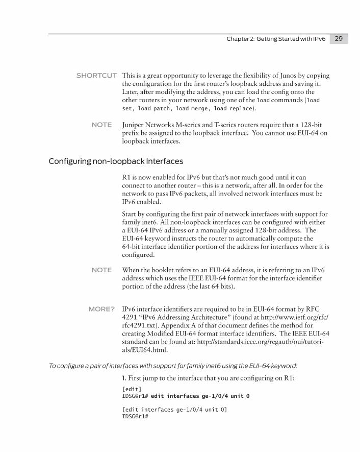
SHORTCUT This is a great opportunity to leverage the flexibility of Junos by copying the configuration for the first router’s loopback address and saving it. Later, after modifying the address, you can load the config onto the other routers in your network using one of the load commands (load set, load patch, load merge, load replace).
NOTE Juniper Networks M-series and T-series routers require that a 128-bit prefix be assigned to the loopback interface. You cannot use EUI-64 on loopback interfaces.
Configuring non-loopback Interfaces
R1 is now enabled for IPv6 but that’s not much good until it can connect to another router – this is a network, after all. In order for the network to pass IPv6 packets, all involved network interfaces must be IPv6 enabled.
Start by configuring the first pair of network interfaces with support for family inet6. All non-loopback interfaces can be configured with either a EUI-64 IPv6 address or a manually assigned 128-bit address. The EUI-64 keyword instructs the router to automatically compute the 64-bit interface identifier portion of the address for interfaces where it is configured.
NOTE When the booklet refers to an EUI-64 address, it is referring to an IPv6 address which uses the IEEE EUI-64 format for the interface identifier portion of the address (the last 64 bits).
MORE? IPv6 interface identifiers are required to be in EUI-64 format by RFC 4291 “IPv6 Addressing Architecture” (found at http://www.ietf.org/rfc/rfc4291.txt). Appendix A of that document defines the method for creating Modified EUI-64 format interface identifiers. The IEEE EUI-64 standard can be found at: http://standards.ieee.org/regauth/oui/tutori-als/EUI64.html.
To configure a pair of interfaces with support for family inet6 using the EUI-64 keyword:
1. First jump to the interface that you are configuring on R1:
[edit]IDSG@r1# edit interfaces ge-1/0/4 unit 0
[edit interfaces ge-1/0/4 unit 0]IDSG@r1#
30 Day One: Exploring IPv6
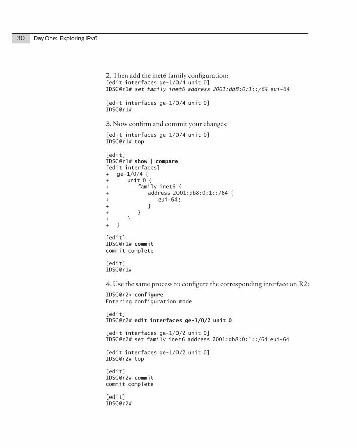
2. Then add the inet6 family configuration:[edit interfaces ge-1/0/4 unit 0]IDSG@r1# set family inet6 address 2001:db8:0:1::/64 eui-64
[edit interfaces ge-1/0/4 unit 0]IDSG@r1#
3. Now confirm and commit your changes:
[edit interfaces ge-1/0/4 unit 0]IDSG@r1# top
[edit]IDSG@r1# show | compare [edit interfaces]+ ge-1/0/4 {+ unit 0 {+ family inet6 {+ address 2001:db8:0:1::/64 {+ eui-64;+ }+ }+ }+ }
[edit]IDSG@r1# commit commit complete
[edit]IDSG@r1#
4. Use the same process to configure the corresponding interface on R2:
IDSG@r2> configure Entering configuration mode
[edit]IDSG@r2# edit interfaces ge-1/0/2 unit 0
[edit interfaces ge-1/0/2 unit 0]IDSG@r2# set family inet6 address 2001:db8:0:1::/64 eui-64
[edit interfaces ge-1/0/2 unit 0]IDSG@r2# top
[edit]IDSG@r2# commit commit complete
[edit]IDSG@r2#
Chapter 2: Getting Started with IPv6 31
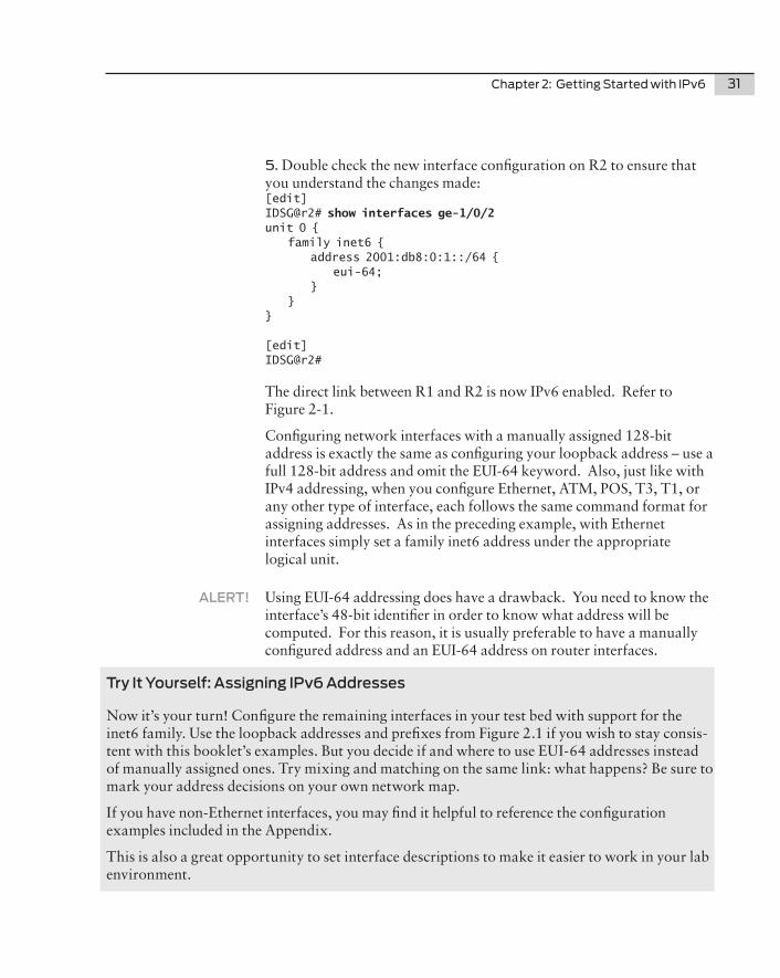
5. Double check the new interface configuration on R2 to ensure that you understand the changes made:[edit]IDSG@r2# show interfaces ge-1/0/2 unit 0 { family inet6 { address 2001:db8:0:1::/64 { eui-64; } }}
[edit]IDSG@r2#
The direct link between R1 and R2 is now IPv6 enabled. Refer to Figure 2-1.
Configuring network interfaces with a manually assigned 128-bit address is exactly the same as configuring your loopback address – use a full 128-bit address and omit the EUI-64 keyword. Also, just like with IPv4 addressing, when you configure Ethernet, ATM, POS, T3, T1, or any other type of interface, each follows the same command format for assigning addresses. As in the preceding example, with Ethernet interfaces simply set a family inet6 address under the appropriate logical unit.
ALERT! Using EUI-64 addressing does have a drawback. You need to know the interface’s 48-bit identifier in order to know what address will be computed. For this reason, it is usually preferable to have a manually configured address and an EUI-64 address on router interfaces.
Try It Yourself: Assigning IPv6 Addresses
Now it’s your turn! Configure the remaining interfaces in your test bed with support for the inet6 family. Use the loopback addresses and prefixes from Figure 2.1 if you wish to stay consis-tent with this booklet’s examples. But you decide if and where to use EUI-64 addresses instead of manually assigned ones. Try mixing and matching on the same link: what happens? Be sure to mark your address decisions on your own network map.
If you have non-Ethernet interfaces, you may find it helpful to reference the configuration examples included in the Appendix.
This is also a great opportunity to set interface descriptions to make it easier to work in your lab environment.
32 Day One: Exploring IPv6
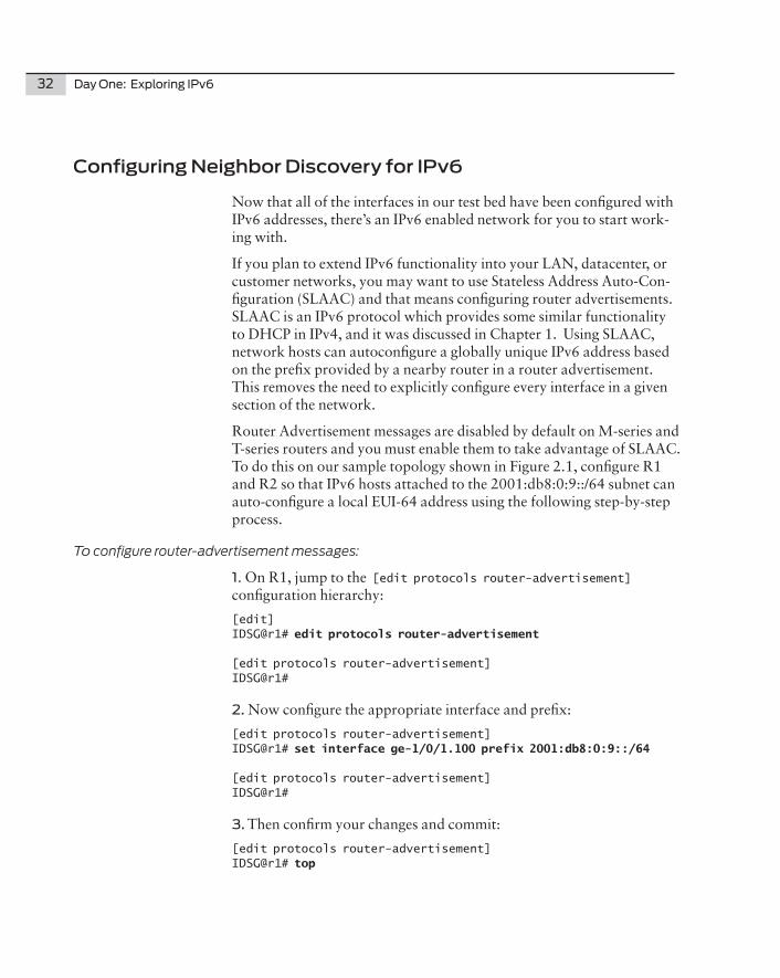
Configuring Neighbor Discovery for IPv6
Now that all of the interfaces in our test bed have been configured with IPv6 addresses, there’s an IPv6 enabled network for you to start work-ing with.
If you plan to extend IPv6 functionality into your LAN, datacenter, or customer networks, you may want to use Stateless Address Auto-Con-figuration (SLAAC) and that means configuring router advertisements. SLAAC is an IPv6 protocol which provides some similar functionality to DHCP in IPv4, and it was discussed in Chapter 1. Using SLAAC, network hosts can autoconfigure a globally unique IPv6 address based on the prefix provided by a nearby router in a router advertisement. This removes the need to explicitly configure every interface in a given section of the network.
Router Advertisement messages are disabled by default on M-series and T-series routers and you must enable them to take advantage of SLAAC. To do this on our sample topology shown in Figure 2.1, configure R1 and R2 so that IPv6 hosts attached to the 2001:db8:0:9::/64 subnet can auto-configure a local EUI-64 address using the following step-by-step process.
To configure router-advertisement messages:
1. On R1, jump to the [edit protocols router-advertisement] configuration hierarchy:
[edit protocols router-advertisement]IDSG@r2# set interface ge-1/0/1.100 prefix 2001:db8:0:9::/64
[edit protocols router-advertisement]IDSG@r2# top
[edit]IDSG@r2# commit commit complete
[edit]IDSG@r2#
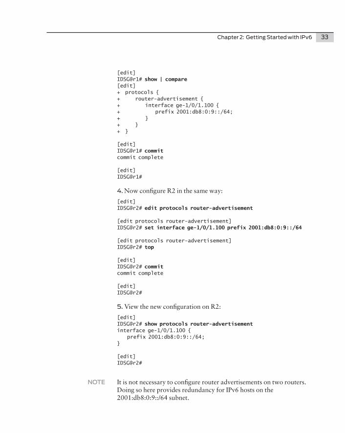
5. View the new configuration on R2:
[edit]IDSG@r2# show protocols router-advertisement interface ge-1/0/1.100 { prefix 2001:db8:0:9::/64;}
[edit]IDSG@r2#
NOTE It is not necessary to configure router advertisements on two routers. Doing so here provides redundancy for IPv6 hosts on the 2001:db8:0:9::/64 subnet.
34 Day One: Exploring IPv6
MORE? To find out more, go to RFC 4861 “Neighbor Discovery for IP Version 6 (IPv6),” and RFC 4862 “IPv6 Stateless Address Autoconfiguration.”
Basic IPv6 Verification and Testing
With the baseline IPv6 configuration in place, it’s time to turn your attention to testing and verification. Start with address verification to ensure that your interfaces are configured properly and that IPv6 traffic can actually transit the configured links, then move on to verification of the router advertisements on R1 and R2.
BEST PRACTICE When configuring any network, it is a very good idea to stop and test your work whenever possible. This ensures easy troubleshooting by isolating the changes you made in each incremental step, and is especially true when working with a new unfamiliar protocol.
IPv6 Address Verification
The procedure used in IPv6 address verification is very similar to the one you likely use for IPv4 addressing, except for the final step:
Confirm the correct association of IPv6 address to network interface by using the show interface commands.
Conduct ping testing to verify that each pair of routers shares a common subnet and that no “fat finger” mistakes have been made.
Review the IPv6 neighbor cache; this final verification differs from IPv4 because IPv6 does not use ARP.
Before conducting any ping or traceroute testing, it is always best practice to verify the addresses assigned to each interface. This is especially true when dealing with IPv6 because of EUI-64 addressing and the longer address format. It’s also important to know that your interfaces are in fact up!
BEST PRACTICE When working with IPv6 addresses, the author highly recommends forming a habit of copying and pasting addresses. With 128 bits and hexadecimal notation, it is extremely easy to mistype an address, potentially causing wasted time troubleshooting non-existent prob-lems.
Chapter 2: Getting Started with IPv6 35
How to confirm correct association of IPv6 addesses
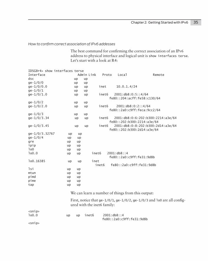
The best command for confirming the correct association of an IPv6 address to physical interface and logical unit is show interfaces terse. Let’s start with a look at R4:
IDSG@r4> show interfaces terse Interface Admin Link Proto Local Remotedsc up up ge-1/0/0 up up ge-1/0/0.0 up up inet 10.0.1.4/24 ge-1/0/1 up up ge-1/0/1.0 up up inet6 2001:db8:0:5::4/64 fe80::204:acff:fe58:c130/64ge-1/0/2 up up ge-1/0/2.0 up up inet6 2001:db8:0:2::4/64 fe80::2a0:c9ff:feca:9cc2/64ge-1/0/3 up up ge-1/0/3.34 up up inet6 2001:db8:0:6:202:b300:2214:a3e/64 fe80::202:b300:2214:a3e/64ge-1/0/3.45 up up inet6 2001:db8:0:8:202:b300:2d14:a3e/64 fe80::202:b300:2d14:a3e/64ge-1/0/3.32767 up up ge-1/0/4 up up gre up up ipip up up lo0 up up lo0.0 up up inet6 2001:db8::4 fe80::2a0:c9ff:fe31:9d8blo0.16385 up up inet inet6 fe80::2a0:c9ff:fe31:9d8blsi up up mtun up up pimd up up pime up up tap up up
We can learn a number of things from this output:
First, notice that ge-1/0/1, ge-1/0/2, ge-1/0/3 and lo0 are all config-ured with the inet6 family:
<snip>lo0.0 up up inet6 2001:db8::4 fe80::2a0:c9ff:fe31:9d8b<snip>
36 Day One: Exploring IPv6
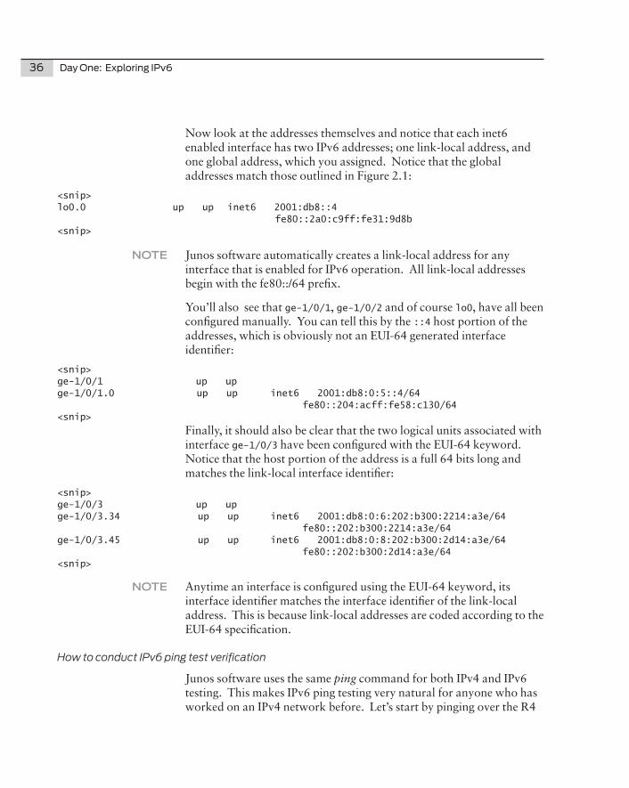
Now look at the addresses themselves and notice that each inet6 enabled interface has two IPv6 addresses; one link-local address, and one global address, which you assigned. Notice that the global addresses match those outlined in Figure 2.1:
<snip>lo0.0 up up inet6 2001:db8::4 fe80::2a0:c9ff:fe31:9d8b<snip>
NOTE Junos software automatically creates a link-local address for any interface that is enabled for IPv6 operation. All link-local addresses begin with the fe80::/64 prefix.
You’ll also see that ge-1/0/1, ge-1/0/2 and of course lo0, have all been configured manually. You can tell this by the ::4 host portion of the addresses, which is obviously not an EUI-64 generated interface identifier:
<snip>ge-1/0/1 up up ge-1/0/1.0 up up inet6 2001:db8:0:5::4/64 fe80::204:acff:fe58:c130/64<snip>
Finally, it should also be clear that the two logical units associated with interface ge-1/0/3 have been configured with the EUI-64 keyword. Notice that the host portion of the address is a full 64 bits long and matches the link-local interface identifier:
<snip>ge-1/0/3 up up ge-1/0/3.34 up up inet6 2001:db8:0:6:202:b300:2214:a3e/64 fe80::202:b300:2214:a3e/64ge-1/0/3.45 up up inet6 2001:db8:0:8:202:b300:2d14:a3e/64 fe80::202:b300:2d14:a3e/64<snip>
NOTE Anytime an interface is configured using the EUI-64 keyword, its interface identifier matches the interface identifier of the link-local address. This is because link-local addresses are coded according to the EUI-64 specification.
How to conduct IPv6 ping test verification
Junos software uses the same ping command for both IPv4 and IPv6 testing. This makes IPv6 ping testing very natural for anyone who has worked on an IPv4 network before. Let’s start by pinging over the R4
Chapter 2: Getting Started with IPv6 37
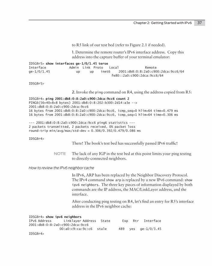
to R5 link of our test bed (refer to Figure 2.1 if needed).
1. Determine the remote router’s IPv6 interface address. Copy this address into the capture buffer of your terminal emulator:
IDSG@r5> show interfaces ge-1/0/1.45 terse Interface Admin Link Proto Local Remotege-1/0/1.45 up up inet6 2001:db8:0:8:2a0:c900:2dca:9cc6/64 fe80::2a0:c900:2dca:9cc6/64
IDSG@r5>
2. Invoke the ping command on R4, using the address copied from R5:
IDSG@r4> ping 2001:db8:0:8:2a0:c900:2dca:9cc6 count 2 PING6(56=40+8+8 bytes) 2001:db8:0:8:202:b300:2d14:a3e --> 2001:db8:0:8:2a0:c900:2dca:9cc616 bytes from 2001:db8:0:8:2a0:c900:2dca:9cc6, icmp_seq=0 hlim=64 time=0.479 ms16 bytes from 2001:db8:0:8:2a0:c900:2dca:9cc6, icmp_seq=1 hlim=64 time=0.306 ms
There! The book’s test bed has successfully passed IPv6 traffic!
NOTE The lack of any IGP in the test bed at this point limits your ping testing to directly-connected neighbors.
How to review the IPv6 neighbor cache
In IPv6, ARP has been replaced by the Neighbor Discovery Protocol. The IPv4 command show arp is replaced by a new IPv6 command: show ipv6 neighbors. The three key pieces of information displayed by both commands are the IP address, the MAC/LinkLayer address, and the interface.
After conducting ping testing on R4, let’s find an entry for R5’s interface address in the IPv6 neighbor cache:
IDSG@r4> show ipv6 neighbors IPv6 Address Linklayer Address State Exp Rtr Interface2001:db8:0:8:2a0:c900:2dca:9cc6 00:a0:c9:ca:9c:c6 stale 489 yes ge-1/0/3.45
IDSG@r4>
38 Day One: Exploring IPv6
Try It Yourself: Verifying IPv6 Addresses
Go through your entire test bed and verify all of your IPv6 interfaces and links. Use the follow-ing commands to ensure that your baseline configurations are correct and complete: show interfaces terse ping show ipv6 neighbor
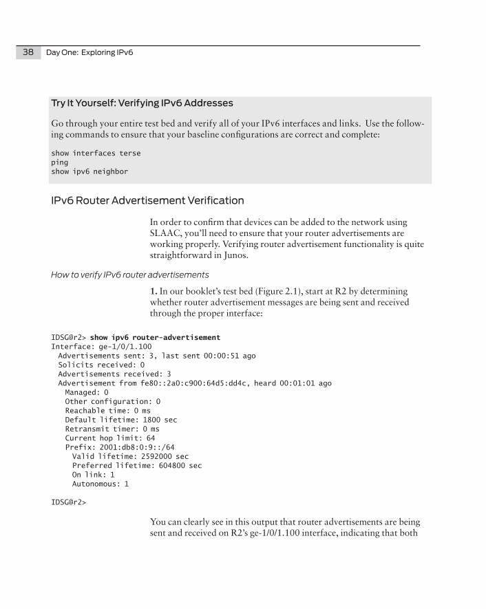
IPv6 Router Advertisement Verification
In order to confirm that devices can be added to the network using SLAAC, you’ll need to ensure that your router advertisements are working properly. Verifying router advertisement functionality is quite straightforward in Junos.
How to verify IPv6 router advertisements
1. In our booklet’s test bed (Figure 2.1), start at R2 by determining whether router advertisement messages are being sent and received through the proper interface:
IDSG@r2> show ipv6 router-advertisement Interface: ge-1/0/1.100 Advertisements sent: 3, last sent 00:00:51 ago Solicits received: 0 Advertisements received: 3 Advertisement from fe80::2a0:c900:64d5:dd4c, heard 00:01:01 ago Managed: 0 Other configuration: 0 Reachable time: 0 ms Default lifetime: 1800 sec Retransmit timer: 0 ms Current hop limit: 64 Prefix: 2001:db8:0:9::/64 Valid lifetime: 2592000 sec Preferred lifetime: 604800 sec On link: 1 Autonomous: 1
IDSG@r2>
You can clearly see in this output that router advertisements are being sent and received on R2’s ge-1/0/1.100 interface, indicating that both
Chapter 2: Getting Started with IPv6 39
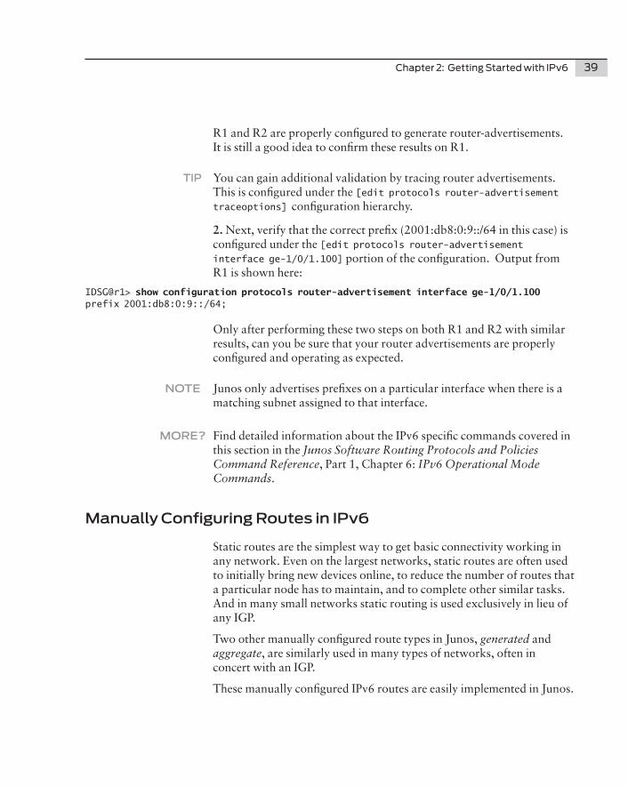
R1 and R2 are properly configured to generate router-advertisements. It is still a good idea to confirm these results on R1.
TIP You can gain additional validation by tracing router advertisements. This is configured under the [edit protocols router-advertisement traceoptions] configuration hierarchy.
2. Next, verify that the correct prefix (2001:db8:0:9::/64 in this case) is configured under the [edit protocols router-advertisement interface ge-1/0/1.100] portion of the configuration. Output from R1 is shown here:
IDSG@r1> show configuration protocols router-advertisement interface ge-1/0/1.100 prefix 2001:db8:0:9::/64;
Only after performing these two steps on both R1 and R2 with similar results, can you be sure that your router advertisements are properly configured and operating as expected.
NOTE Junos only advertises prefixes on a particular interface when there is a matching subnet assigned to that interface.
MORE? Find detailed information about the IPv6 specific commands covered in this section in the Junos Software Routing Protocols and Policies Command Reference, Part 1, Chapter 6: IPv6 Operational Mode Commands.
Manually Configuring Routes in IPv6
Static routes are the simplest way to get basic connectivity working in any network. Even on the largest networks, static routes are often used to initially bring new devices online, to reduce the number of routes that a particular node has to maintain, and to complete other similar tasks. And in many small networks static routing is used exclusively in lieu of any IGP.
Two other manually configured route types in Junos, generated and aggregate, are similarly used in many types of networks, often in concert with an IGP.
These manually configured IPv6 routes are easily implemented in Junos.
40 Day One: Exploring IPv6
Configuring Static, Aggregate, and Generated IPv6 Routes
The Junos OS maintains multiple routing tables for various protocols. If you have used MPLS, VPN’s, or multicast in Junos, you are likely already familiar with this behavior.
The default routing table is inet.0, which is the default IPv4 unicast routing table. There is a default IPv6 unicast routing table as well, and it is inet6.0. To configure IPv6 routes in Junos you must add the routes to the inet6.0 RIB (Routing Information Base). To do this you must configure IPv6 routes in a separate branch of the configuration hierarchy from IPv4 routes.
MORE? There are seven default routing tables maintained by Junos Software. You can read more here: http://www.juniper.net/techpubs/software/Junos/Junos94/swconfig-routing/Junos-routing-tables.html.
The following step-by-step sections show how to configure static, aggregate, and generated IPv6 routes.
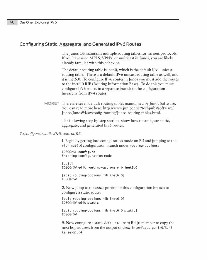
To configure a static IPv6 route on R5:
1. Begin by getting into configuration mode on R5 and jumping to the rib inet6.0 configuration branch under routing-options:
IDSG@r5> configure Entering configuration mode
[edit]IDSG@r5# edit routing-options rib inet6.0
[edit routing-options rib inet6.0]IDSG@r5#
2. Now jump to the static portion of this configuration branch to configure a static route:
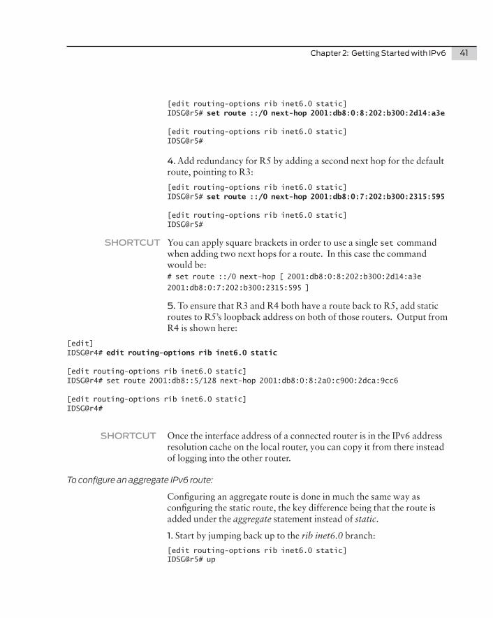
3. Now configure a static default route to R4 (remember to copy the next hop address from the output of show interfaces ge-1/0/3.45 terse on R4):
Chapter 2: Getting Started with IPv6 41
[edit routing-options rib inet6.0 static]IDSG@r5# set route ::/0 next-hop 2001:db8:0:8:202:b300:2d14:a3e
[edit routing-options rib inet6.0 static]IDSG@r5#
4. Add redundancy for R5 by adding a second next hop for the default route, pointing to R3:
[edit routing-options rib inet6.0 static]IDSG@r5# set route ::/0 next-hop 2001:db8:0:7:202:b300:2315:595
[edit routing-options rib inet6.0 static]IDSG@r5#
SHORTCUT You can apply square brackets in order to use a single set command when adding two next hops for a route. In this case the command would be: # set route ::/0 next-hop [ 2001:db8:0:8:202:b300:2d14:a3e
2001:db8:0:7:202:b300:2315:595 ]
5. To ensure that R3 and R4 both have a route back to R5, add static routes to R5’s loopback address on both of those routers. Output from R4 is shown here:
[edit routing-options rib inet6.0 static]IDSG@r4# set route 2001:db8::5/128 next-hop 2001:db8:0:8:2a0:c900:2dca:9cc6
[edit routing-options rib inet6.0 static]IDSG@r4#
SHORTCUT Once the interface address of a connected router is in the IPv6 address resolution cache on the local router, you can copy it from there instead of logging into the other router.
To configure an aggregate IPv6 route:
Configuring an aggregate route is done in much the same way as configuring the static route, the key difference being that the route is added under the aggregate statement instead of static.
1. Start by jumping back up to the rib inet6.0 branch:
[edit routing-options rib inet6.0 static]IDSG@r5# up
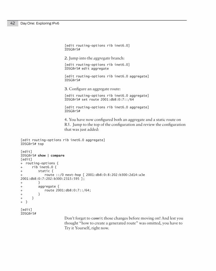
4. You have now configured both an aggregate and a static route on R5. Jump to the top of the configuration and review the configuration that was just added:
[edit routing-options rib inet6.0 aggregate]IDSG@r5# top
Don’t forget to commit those changes before moving on! And lest you thought “how to create a generated route” was omitted, you have to Try it Yourself, right now.
Chapter 2: Getting Started with IPv6 43
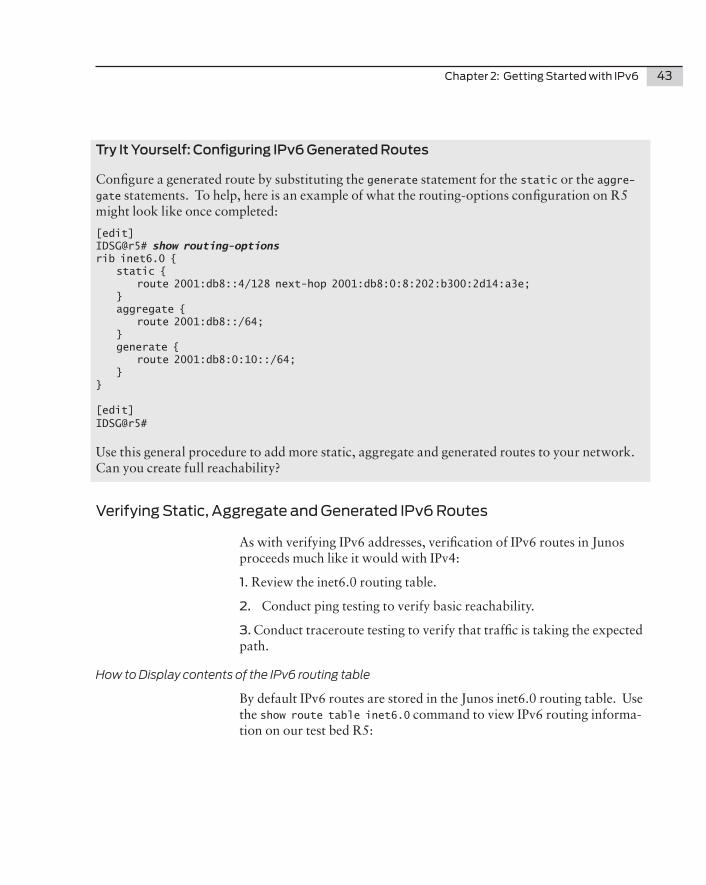
Try It Yourself: Configuring IPv6 Generated Routes
Configure a generated route by substituting the generate statement for the static or the aggre-gate statements. To help, here is an example of what the routing-options configuration on R5 might look like once completed:
Use this general procedure to add more static, aggregate and generated routes to your network. Can you create full reachability?
Verifying Static, Aggregate and Generated IPv6 Routes
As with verifying IPv6 addresses, verification of IPv6 routes in Junos proceeds much like it would with IPv4:
1. Review the inet6.0 routing table.
2.Conduct ping testing to verify basic reachability.
3. Conduct traceroute testing to verify that traffic is taking the expected path.
How to Display contents of the IPv6 routing table
By default IPv6 routes are stored in the Junos inet6.0 routing table. Use the show route table inet6.0 command to view IPv6 routing informa-tion on our test bed R5:
44 Day One: Exploring IPv6
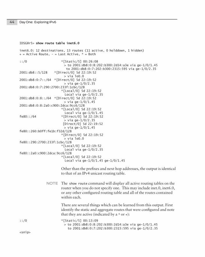
IDSG@r5> show route table inet6.0
inet6.0: 12 destinations, 13 routes (11 active, 0 holddown, 1 hidden)+ = Active Route, - = Last Active, * = Both
::/0 *[Static/5] 00:26:08 > to 2001:db8:0:8:202:b300:2d14:a3e via ge-1/0/1.45 to 2001:db8:0:7:202:b300:2315:595 via ge-1/0/2.352001:db8::5/128 *[Direct/0] 5d 22:19:52 > via lo0.02001:db8:0:7::/64 *[Direct/0] 5d 22:19:52 > via ge-1/0/2.352001:db8:0:7:290:2700:233f:1cbc/128 *[Local/0] 5d 22:19:52 Local via ge-1/0/2.352001:db8:0:8::/64 *[Direct/0] 5d 22:19:52 > via ge-1/0/1.452001:db8:0:8:2a0:c900:2dca:9cc6/128 *[Local/0] 5d 22:19:52 Local via ge-1/0/1.45fe80::/64 *[Direct/0] 5d 22:19:52 > via ge-1/0/2.35 [Direct/0] 5d 22:19:52 > via ge-1/0/1.45fe80::260:b0ff:fe1b:f32d/128 *[Direct/0] 5d 22:19:52 > via lo0.0fe80::290:2700:233f:1cbc/128 *[Local/0] 5d 22:19:52 Local via ge-1/0/2.35fe80::2a0:c900:2dca:9cc6/128 *[Local/0] 5d 22:19:52 Local via ge-1/0/1.45 ge-1/0/1.45
Other than the prefixes and next hop addresses, the output is identical to that of an IPv4 unicast routing table.
NOTE The show route command will display all active routing tables on the router when you do not specify one. This may include inet.0, inet6.0, or any other configured routing table and all of the routes contained within each.
There are several things which can be learned from this output. First identify the static and aggregate routes that were configured and note that they are active (indicated by a * or +):
::/0 *[Static/5] 00:13:09 > to 2001:db8:0:8:202:b300:2d14:a3e via ge-1/0/1.45 to 2001:db8:0:7:202:b300:2315:595 via ge-1/0/2.35<snip>
Next, you can see that the next hop is what you expect for each route. Note that the static default route does list both configured next-hops and that the selected path is via ge-1/0/1.45 to R4:
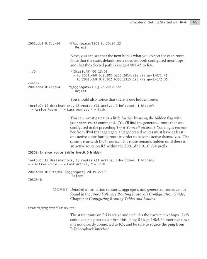
::/0 *[Static/5] 00:13:09 > to 2001:db8:0:8:202:b300:2d14:a3e via ge-1/0/1.45 to 2001:db8:0:7:202:b300:2315:595 via ge-1/0/2.35<snip>2001:db8:0:7::/64 *[Aggregate/130] 2d 20:20:22 Reject
You should also notice that there is one hidden route:
inet6.0: 12 destinations, 13 routes (11 active, 0 holddown, 1 hidden)+ = Active Route, - = Last Active, * = Both
You can investigate this a little further by using the hidden flag with your show route command. (You’ll find the generated route that was configured in the preceding Try it Yourself section.) You might remem-ber from IPv4 that aggregate and generated routes must have at least one active contributing route in order to become active themselves. The same is true with IPv6 routes. This route remains hidden until there is an active route on R5 within the 2001:db8:0:10::/64 prefix:
IDSG@r5> show route table inet6.0 hidden
inet6.0: 12 destinations, 13 routes (11 active, 0 holddown, 1 hidden)+ = Active Route, - = Last Active, * = Both
MORE? Detailed information on static, aggregate, and generated routes can be found in the Junos Software Routing Protocols Configuration Guide, Chapter 4: Configuring Routing Tables and Routes.
How to ping test IPv6 routes:
The static route on R5 is active and includes the correct next hops. Let’s conduct a ping test to confirm this. Ping R3’s ge-1/0/4.34 interface since it is not directly connected to R5, and be sure to source the ping from R5’s loopback interface:
46 Day One: Exploring IPv6
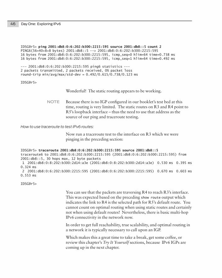
IDSG@r5> ping 2001:db8:0:6:202:b300:2215:595 source 2001:db8::5 count 2 PING6(56=40+8+8 bytes) 2001:db8::5 --> 2001:db8:0:6:202:b300:2215:59516 bytes from 2001:db8:0:6:202:b300:2215:595, icmp_seq=0 hlim=64 time=0.738 ms16 bytes from 2001:db8:0:6:202:b300:2215:595, icmp_seq=1 hlim=64 time=0.492 ms
Wonderful! The static routing appears to be working.
NOTE Because there is no IGP configured in our booklet’s test bed at this time, routing is very limited. The static routes on R3 and R4 point to R5’s loopback interface – thus the need to use that address as the source of our ping and traceroute testing.
How to use traceroute to test IPv6 routes:
Now run a traceroute test to the interface on R3 which we were pinging in the preceding section:
IDSG@r5> traceroute 2001:db8:0:6:202:b300:2215:595 source 2001:db8::5 traceroute6 to 2001:db8:0:6:202:b300:2215:595 (2001:db8:0:6:202:b300:2215:595) from 2001:db8::5, 30 hops max, 12 byte packets 1 2001:db8:0:8:202:b300:2d14:a3e (2001:db8:0:8:202:b300:2d14:a3e) 0.530 ms 0.395 ms 0.324 ms 2 2001:db8:0:6:202:b300:2215:595 (2001:db8:0:6:202:b300:2215:595) 0.670 ms 0.603 ms 0.553 ms
IDSG@r5>
You can see that the packets are traversing R4 to reach R3’s interface. This was expected based on the preceding show route output which indicates the link to R4 is the selected path for R5’s default route. You cannot count on optimal routing when using static routes and certainly not when using default routes! Nevertheless, there is basic multi-hop IPv6 connectivity in the network now.
In order to get full reachability, true scalability, and optimal routing in a network it is typically necessary to call upon an IGP.
Which makes this a great time to take a break, get some coffee, or review this chapter’s Try It Yourself sections, because IPv6 IGPs are coming up in the next chapter.
In the last chapter you learned the basics of configuring IPv6 using the Junos operating system. For small enterprise networks composed of a couple of network devices and a handful of prefixes, this may be everything you need to know to roll out IPv6. Larger and more complex networks need to leverage a dynamic routing protocol, but if you’re small, stick around. There’s a lot to learn for everyone.
In this chapter you will learn about all three Interior Gateway Proto-cols (IGPs) that support IPv6: RIPng, OSPF3, and IS-IS, using the lessons and tools covered in Chapter 2. After reading this chapter you’ll know how to enable and verify the operation of basic dynamic IPv6 routing within your network using your choice of IGP, not to mention enhancing your overall understanding of routing IPv6 in Junos.
NOTE This chapter assumes that you have experience with dynamic routing in IPv4 and at least a basic understanding of IGP routing. If you feel you need more information on Interior Gateway Protocols, see Part 5 of the Junos Software Routing Protocols Configuration Guide avail-able at www.juniper.net/techpubs.
Introduction to IPv6 Routing Protocols
If you are using a dynamic routing protocol in your current IPv4 network, then you probably need to configure an IPv6 IGP as well. If you are configuring a new IPv6-only network, it’s a great idea to incorporate a routing protocol into your design now, regardless of its size, to allow for future growth of the network.
There are three IGPs to choose from when selecting an IPv6 routing protocol in Junos: RIPng, OSPF3 and IS-IS. All three of these protocols should be familiar to you from your work with similar IPv4 routing protocols, and the steps needed to configure them for IPv6 are almost identical (and actually are identical in some cases). However both RIPng and OSPF3 require configuring the new versions to support IPv6, while IS-IS does not.
ALERT! RIP and OSPF require new versions to support IPv6.
If you have an existing IPv4 network that is using an IGP, it may be wise to select the same protocol for your IPv6 network. This minimizes the number of changes and new pieces that you and your networking
Chapter 3: Dynamic Routing with IPv6 49
staff must learn. On the other hand, adding IPv6 to your network is a great time to reconsider your current routing protocol and network topology and seek to optimize both for your current and future needs.
Ultimately, the IGP you choose must meet the specific needs of your network and your business. After reading these sections you should have a solid understanding of all three protocols and be better equipped to choose one. If you have already decided on an IGP, feel free to jump directly to that section.
MORE? For a truly informed discussion on choosing an IGP, take a look at Jeff Doyle’s book, OSPF and IS-IS: Choosing an IGP for Large-Scale Networks (Addison-Wesley, 2007) at www.juniper.net/books.
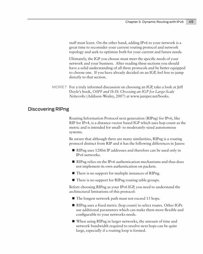
Discovering RIPng
Routing Information Protocol next generation (RIPng) for IPv6, like RIP for IPv4, is a distance-vector based IGP which uses hop count as the metric and is intended for small- to moderately-sized autonomous systems.
Be aware that although there are many similarities, RIPng is a routing protocol distinct from RIP and it has the following differences in Junos:
n RIPng uses 128bit IP addresses and therefore can be used only in IPv6 networks.
n RIPng relies on the IPv6 authentication mechanisms and thus does not implement its own authentication on packets.
n There is no support for multiple instances of RIPng.
n There is no support for RIPng routing table groups.
Before choosing RIPng as your IPv6 IGP, you need to understand the architectural limitations of this protocol:
n The longest network path must not exceed 15 hops.
n RIPng uses a fixed metric (hop count) to select routes. Other IGPs use additional parameters which can make them more flexible and configurable to your networks needs.
n When using RIPng in larger networks, the amount of time and network bandwidth required to resolve next hops can be quite large, especially if a routing loop is formed.
50 Day One: Exploring IPv6
MORE? To To learn more about RIPng, see RFC 2080: RIPng for IPv6 (http://tools.ietf.org/rfc/rfc2080.txt) and RFC 2081: RIPng Protocol Applica-bility Statement (http://tools.ietf.org/rfc/rfc2081.txt).
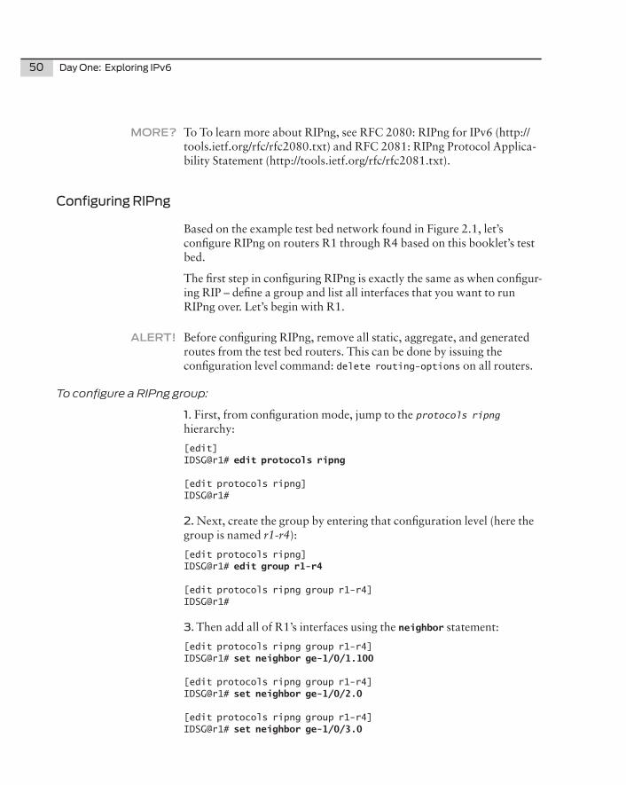
Configuring RIPng
Based on the example test bed network found in Figure 2.1, let’s configure RIPng on routers R1 through R4 based on this booklet’s test bed.
The first step in configuring RIPng is exactly the same as when configur-ing RIP – define a group and list all interfaces that you want to run RIPng over. Let’s begin with R1.
ALERT! Before configuring RIPng, remove all static, aggregate, and generated routes from the test bed routers. This can be done by issuing the configuration level command: delete routing-options on all routers.
To configure a RIPng group:
1. First, from configuration mode, jump to the protocols ripng hierarchy:
[edit]IDSG@r1# edit protocols ripng
[edit protocols ripng]IDSG@r1#
2. Next, create the group by entering that configuration level (here the group is named r1-r4):
[edit protocols ripng]IDSG@r1# edit group r1-r4
[edit protocols ripng group r1-r4]IDSG@r1#
3. Then add all of R1’s interfaces using the neighbor statement:
[edit protocols ripng group r1-r4]IDSG@r1# set neighbor ge-1/0/1.100
[edit protocols ripng group r1-r4]IDSG@r1# set neighbor ge-1/0/2.0
[edit protocols ripng group r1-r4]IDSG@r1# set neighbor ge-1/0/3.0
50
Chapter 3: Dynamic Routing with IPv6 51
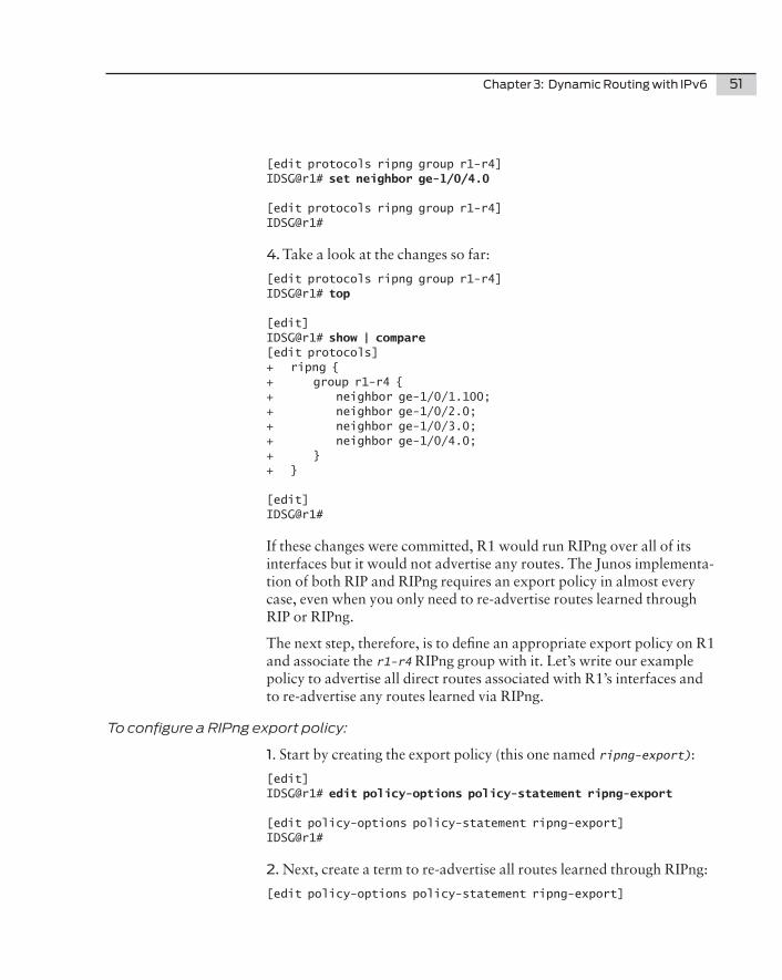
[edit protocols ripng group r1-r4]IDSG@r1# set neighbor ge-1/0/4.0
If these changes were committed, R1 would run RIPng over all of its interfaces but it would not advertise any routes. The Junos implementa-tion of both RIP and RIPng requires an export policy in almost every case, even when you only need to re-advertise routes learned through RIP or RIPng.
The next step, therefore, is to define an appropriate export policy on R1 and associate the r1-r4 RIPng group with it. Let’s write our example policy to advertise all direct routes associated with R1’s interfaces and to re-advertise any routes learned via RIPng.
To configure a RIPng export policy:
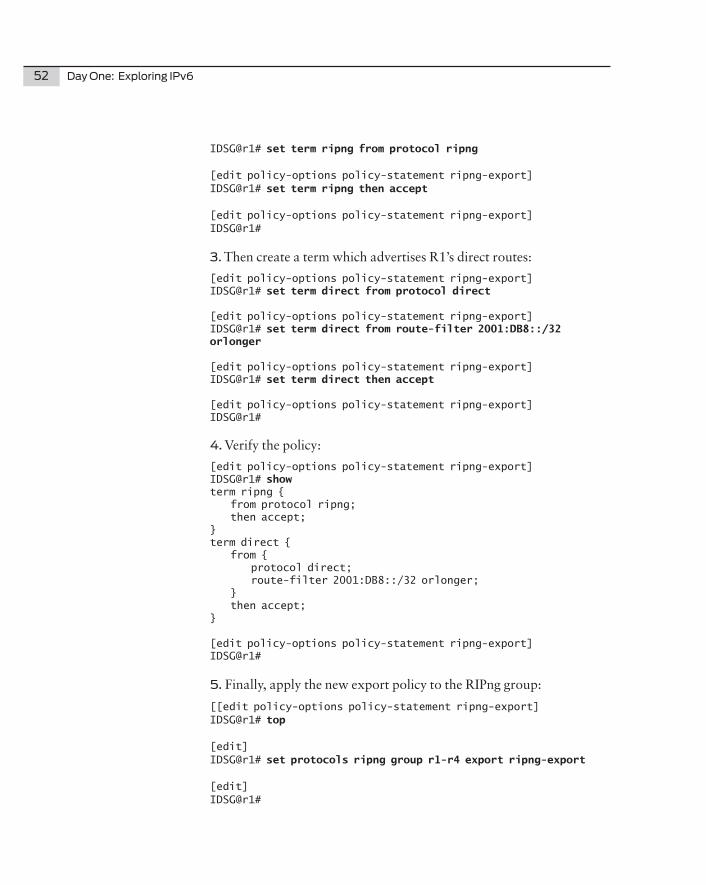
1. Start by creating the export policy (this one named ripng-export):
[edit policy-options policy-statement ripng-export]IDSG@r1# show term ripng { from protocol ripng; then accept;}term direct { from { protocol direct; route-filter 2001:DB8::/32 orlonger; } then accept;}
5. Finally, apply the new export policy to the RIPng group:
[[edit policy-options policy-statement ripng-export]IDSG@r1# top
[edit]IDSG@r1# set protocols ripng group r1-r4 export ripng-export
[edit]IDSG@r1#
Chapter 3: Dynamic Routing with IPv6 53
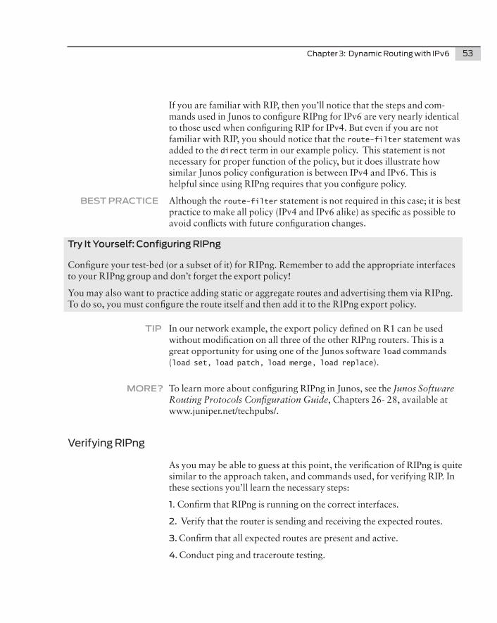
If you are familiar with RIP, then you’ll notice that the steps and com-mands used in Junos to configure RIPng for IPv6 are very nearly identical to those used when configuring RIP for IPv4. But even if you are not familiar with RIP, you should notice that the route-filter statement was added to the direct term in our example policy. This statement is not necessary for proper function of the policy, but it does illustrate how similar Junos policy configuration is between IPv4 and IPv6. This is helpful since using RIPng requires that you configure policy.
BEST PRACTICE Although the route-filter statement is not required in this case; it is best practice to make all policy (IPv4 and IPv6 alike) as specific as possible to avoid conflicts with future configuration changes.
Try It Yourself: Configuring RIPng
Configure your test-bed (or a subset of it) for RIPng. Remember to add the appropriate interfaces to your RIPng group and don’t forget the export policy!
You may also want to practice adding static or aggregate routes and advertising them via RIPng. To do so, you must configure the route itself and then add it to the RIPng export policy.
TIP In our network example, the export policy defined on R1 can be used without modification on all three of the other RIPng routers. This is a great opportunity for using one of the Junos software load commands (load set, load patch, load merge, load replace).
MORE? To learn more about configuring RIPng in Junos, see the Junos Software Routing Protocols Configuration Guide, Chapters 26- 28, available at www.juniper.net/techpubs/.
Verifying RIPng
As you may be able to guess at this point, the verification of RIPng is quite similar to the approach taken, and commands used, for verifying RIP. In these sections you’ll learn the necessary steps:
1. Confirm that RIPng is running on the correct interfaces.
2. Verify that the router is sending and receiving the expected routes.
3. Confirm that all expected routes are present and active.
4. Conduct ping and traceroute testing.
54 Day One: Exploring IPv6
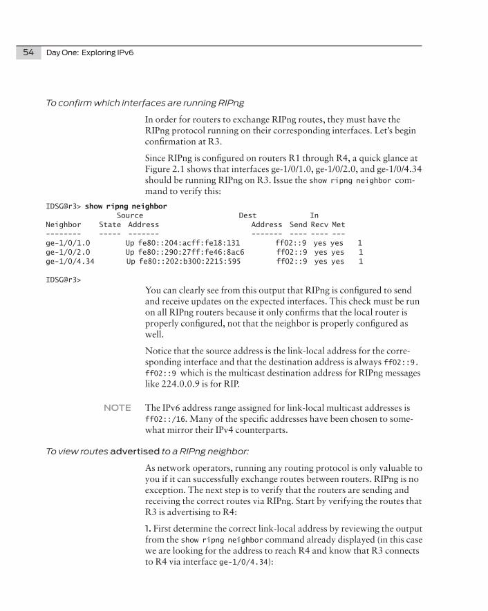
To confirm which interfaces are running RIPng
In order for routers to exchange RIPng routes, they must have the RIPng protocol running on their corresponding interfaces. Let’s begin confirmation at R3.
Since RIPng is configured on routers R1 through R4, a quick glance at Figure 2.1 shows that interfaces ge-1/0/1.0, ge-1/0/2.0, and ge-1/0/4.34 should be running RIPng on R3. Issue the show ripng neighbor com-mand to verify this:
IDSG@r3> show ripng neighbor Source Dest InNeighbor State Address Address Send Recv Met-------- ----- ------- ------- ---- ---- ---ge-1/0/1.0 Up fe80::204:acff:fe18:131 ff02::9 yes yes 1ge-1/0/2.0 Up fe80::290:27ff:fe46:8ac6 ff02::9 yes yes 1ge-1/0/4.34 Up fe80::202:b300:2215:595 ff02::9 yes yes 1
IDSG@r3>
You can clearly see from this output that RIPng is configured to send and receive updates on the expected interfaces. This check must be run on all RIPng routers because it only confirms that the local router is properly configured, not that the neighbor is properly configured as well.
Notice that the source address is the link-local address for the corre-sponding interface and that the destination address is always ff02::9. ff02::9 which is the multicast destination address for RIPng messages like 224.0.0.9 is for RIP.
NOTE The IPv6 address range assigned for link-local multicast addresses is ff02::/16. Many of the specific addresses have been chosen to some-what mirror their IPv4 counterparts.
To view routes advertised to a RIPng neighbor:
As network operators, running any routing protocol is only valuable to you if it can successfully exchange routes between routers. RIPng is no exception. The next step is to verify that the routers are sending and receiving the correct routes via RIPng. Start by verifying the routes that R3 is advertising to R4:
1. First determine the correct link-local address by reviewing the output from the show ripng neighbor command already displayed (in this case we are looking for the address to reach R4 and know that R3 connects to R4 via interface ge-1/0/4.34):
Chapter 3: Dynamic Routing with IPv6 55
Source Dest InNeighbor State Address Address Send Recv Met<snip>ge-1/0/4.34 Up fe80::202:b300:2215:595 ff02::9 yes yes 1
2. Now use that address to issue the show route advertising-protocol ripng command:
IDSG@r3> show route advertising-protocol ripng fe80::202:b300:2215:595
inet6.0: 24 destinations, 30 routes (24 active, 0 holddown, 0 hidden)+ = Active Route, - = Last Active, * = Both
2001:db8::1/128 *[RIPng/100] 01:45:57, metric 2, tag 0 > to fe80::202:b3ff:fe0a:c826 via ge-1/0/2.02001:db8::2/128 *[RIPng/100] 01:45:58, metric 2, tag 0 > to fe80::202:b3ff:fecd:94b0 via ge-1/0/1.02001:db8::3/128 *[Direct/0] 03:56:13 > via lo0.02001:db8:0:1::/64 *[RIPng/100] 01:45:58, metric 2, tag 0 > to fe80::202:b3ff:fecd:94b0 via ge-1/0/1.0 to fe80::202:b3ff:fe0a:c826 via ge-1/0/2.02001:db8:0:3::/64 *[Direct/0] 03:56:13 > via ge-1/0/1.0 [RIPng/100] 01:45:58, metric 2, tag 0 > to fe80::202:b3ff:fecd:94b0 via ge-1/0/1.02001:db8:0:4::/64 *[Direct/0] 03:56:13 > via ge-1/0/2.0 [RIPng/100] 01:45:57, metric 2, tag 0 > to fe80::202:b3ff:fe0a:c826 via ge-1/0/2.02001:db8:0:6::/64 *[Direct/0] 01:36:08 > via ge-1/0/4.34 [RIPng/100] 01:35:15, metric 2, tag 0 > to fe80::202:b300:2214:a3e via ge-1/0/4.342001:db8:0:7::/64 *[Direct/0] 01:36:08 > via ge-1/0/4.352001:db8:0:9::/64 *[RIPng/100] 01:45:58, metric 2, tag 0 to fe80::202:b3ff:fecd:94b0 via ge-1/0/1.0 > to fe80::202:b3ff:fe0a:c826 via ge-1/0/2.0
IDSG@r3>
The output confirms that all direct and RIPng routes are being sent from R3 to R4, based on the configured export policy. One thing to note is that all of the RIPng next hops point to the link-local address of the neighboring router; this is different from IPv4, which has no link-local addressing.
Now let’s verify that R3 is receiving the correct routes from R4.
56 Day One: Exploring IPv6
To view routes received by a RIPng router:
1. Start by capturing the neighbor’s directly connected link-local address (remember that Junos automatically configures link-local addresses for all IPv6 enabled interfaces and that they always begin with the fe80::/64 prefix):
IDSG@r4> show interfaces ge-1/0/3.34 terse Interface Admin Link Proto Local Remotege-1/0/3.34 up up inet6 2001:db8:0:6:202:b300:2214:a3e/64 fe80::202:b300:2214:a3e/64
IDSG@r4>
2. Then use the captured address with the show route receive-protocol ripng command to view received routes:
IDSG@r3> show route receive-protocol ripng fe80::202:b300:2214:a3e
inet6.0: 24 destinations, 30 routes (24 active, 0 holddown, 0 hidden)+ = Active Route, - = Last Active, * = Both
2001:db8::4/128 *[RIPng/100] 02:00:26, metric 2, tag 0 > to fe80::202:b300:2214:a3e via ge-1/0/4.342001:db8:0:2::/64 *[RIPng/100] 02:11:08, metric 2, tag 0 to fe80::202:b3ff:fe0a:c826 via ge-1/0/2.0 > to fe80::202:b300:2214:a3e via ge-1/0/4.342001:db8:0:5::/64 *[RIPng/100] 02:11:09, metric 2, tag 0 > to fe80::202:b3ff:fecd:94b0 via ge-1/0/1.0 to fe80::202:b300:2214:a3e via ge-1/0/4.342001:db8:0:6::/64 [RIPng/100] 02:00:26, metric 2, tag 0 > to fe80::202:b300:2214:a3e via ge-1/0/4.342001:db8:0:8::/64 *[RIPng/100] 02:00:26, metric 2, tag 0 > to fe80::202:b300:2214:a3e via ge-1/0/4.34
R4 is advertising all of its directly connected routes, including its loopback address, to R3. Notice that the RIPng route for 2001:db8:0:6::/64 is not active on R3. This is because R3 has a direct route for this network and direct routes are preferred over all other routes, due to them having an administrative distance of 0.
MORE? For more information on administrative distance and route selection, see the JNCIS-M Study Guide at www.juniper.net/us/en/training/certification/books.html.
Chapter 3: Dynamic Routing with IPv6 57
After verifying these results on all of the RIPng routers, it can be determined that the expected routes are being exchanged by RIPng. This confirms that the export policy ripng-export is working correctly, and that all RIPng routes and direct routes beginning with 2001:DB8::/32 are being advertised by all RIPng routers throughout the network.
To confirm routes by viewing the RIPng route table
The next step to verify the operation of RIPng is to display all of the routes being learned through that protocol on each router. This is accomplished using the show route protocol ripng command, as shown here with the output from R2:
inet6.0: 24 destinations, 31 routes (24 active, 0 holddown, 0 hidden)+ = Active Route, - = Last Active, * = Both
2001:db8::1/128 *[RIPng/100] 00:08:28, metric 2, tag 0 > to fe80::2a0:c900:64d5:dd4c via ge-1/0/1.100 to fe80::202:b3ff:fe14:753 via ge-1/0/2.02001:db8::3/128 *[RIPng/100] 00:08:28, metric 2, tag 0 > to fe80::204:acff:fe18:131 via ge-1/0/3.02001:db8::4/128 *[RIPng/100] 00:08:28, metric 2, tag 0 > to fe80::204:acff:fe58:c130 via ge-1/0/4.02001:db8:0:1::/64 [RIPng/100] 00:08:28, metric 2, tag 0 to fe80::2a0:c900:64d5:dd4c via ge-1/0/1.100 > to fe80::202:b3ff:fe14:753 via ge-1/0/2.02001:db8:0:2::/64 *[RIPng/100] 00:08:28, metric 2, tag 0 to fe80::2a0:c900:64d5:dd4c via ge-1/0/1.100 to fe80::202:b3ff:fe14:753 via ge-1/0/2.0 > to fe80::204:acff:fe58:c130 via ge-1/0/4.02001:db8:0:3::/64 [RIPng/100] 00:08:28, metric 2, tag 0 > to fe80::204:acff:fe18:131 via ge-1/0/3.02001:db8:0:4::/64 *[RIPng/100] 00:08:28, metric 2, tag 0 to fe80::2a0:c900:64d5:dd4c via ge-1/0/1.100 > to fe80::202:b3ff:fe14:753 via ge-1/0/2.0 to fe80::204:acff:fe18:131 via ge-1/0/3.02001:db8:0:5::/64 [RIPng/100] 00:08:28, metric 2, tag 0 > to fe80::204:acff:fe58:c130 via ge-1/0/4.02001:db8:0:6::/64 *[RIPng/100] 00:08:28, metric 2, tag 0 > to fe80::204:acff:fe18:131 via ge-1/0/3.0 to fe80::204:acff:fe58:c130 via ge-1/0/4.02001:db8:0:7::/64 *[RIPng/100] 00:08:28, metric 2, tag 0 > to fe80::204:acff:fe18:131 via ge-1/0/3.02001:db8:0:8::/64 *[RIPng/100] 00:08:28, metric 2, tag 0
58 Day One: Exploring IPv6
> to fe80::204:acff:fe58:c130 via ge-1/0/4.02001:db8:0:9::/64 [RIPng/100] 00:08:28, metric 2, tag 0 > to fe80::2a0:c900:64d5:dd4c via ge-1/0/1.100 to fe80::202:b3ff:fe14:753 via ge-1/0/2.0ff02::9/128 *[RIPng/100] 00:08:28, metric 1 MultiRecv
Referring back to Figure 2.1, this output confirms that RIPng is operating properly in our test bed. All of the interface /64s, as well as, all three of the other RIPng router’s loopback addresses, are being learned via RIPng. You might also notice that all of the routes being learned from R1 have two next hops. This is due to the fact that there are two links connecting R1 and R2 and both of these interfaces have been added to the r1-r4 RIPng group.
NOTE R2’s loopback address is not a RIPng route on R2 because R2 is the only router injecting that route into RIPng, and split horizon prevents the route from being advertised back to R2 from other RIPng routers.
Once these results are confirmed on all routers, it is fairly safe to say that RIPng is properly configured throughout the network, but it’s always a good idea to confirm this with connectivity tests like ping and traceroute. Let’s complete the sequence.
To conduct ping and traceroute testing
Once RIPng is verified to be exchanging the expected routes, it’s time to double-check with connectivity testing.
Just as you did with static routes in Chapter 2, first ping and then traceroute to and from various locations in the network to ensure that IPv6 traffic can, in fact, traverse it.
In this booklet’s test bed, all interface addresses should be reachable from all four RIPng routers except for R5’s loopback address. Since R5 is not participating in the RIPng domain, it would need a static route configured and exported into RIPng on either R3 or R4 (or both) to make its loopback address reachable to the RIPng routers.
MORE? IF you want to learn more about RIPng operational mode commands, see Junos Software Routing Protocols and Policies Command Refer-ence, Chapter 11, at www.juniper.net/techpubs.
Chapter 3: Dynamic Routing with IPv6 59
Try It Yourself: Verifying RIPng
Using the tools and skills you have learned in this section, verify the operation of your RIPng test bed.
Start with show ripng neighbor to confirm that RIPng is operating on the necessary interfaces. Use the show route receive-protocol ripng, show route advertising-protocol ripng and show route protocol ripng to verify the exchange of routes between RIPng routers and then test connectivity and optimal routing with the ping and traceroute commands.
Exploring OSPF3
Unlike RIPng, which is a distinct protocol from RIP, OSPF3 is simply a modified version of OSPF which supports IPv6. OSPF (including OSPFv2 and OSPF3) is an IGP which uses link-state information and the shortest path first (or Dijkstra) algorithm to make routing decisions using interface cost as the metric.
Some of the notable differences between OSPF3 and OSPFv2 include:
n OSPF3 bases all neighbor ID information on a 32-bit router ID.
n OSPF3 runs per link rather than per subnet.
n OSPF3 router and network link-state advertisements (LSAs) do not carry any prefix information.
n OSPF3 includes two new LSA types: the link-LSA and the intra-area-prefix-LSA.
n In OSPF3, type 3 and type 4 summary LSAs have been renamed to inter-area-prefix-LSAs and inter-area-router-LSAs respectively.
n OSPF3 uses link-local addresses for all neighbor exchanges (except virtual links).
n OSPF3 relies on the IPv6 authentication header instead of carrying authentication information within the packet.
Like OSPFv2, OSPF3 quickly detects topological changes in the net-work and calculates new routes swiftly and without much overhead traffic. OSPF3 scales well and is a good choice for networks of almost any size.
MORE? Want to learn more about OSPF3? Check out RFC 5340: OSPF for IPv6 at http://tools.ietf.org/rfc/rfc5340.txt.
60 Day One: Exploring IPv6
Configuring OSPF3
To configure OSPF3 on all five of our test bed routers, as illustrated back in Figure 2.1, the network needs to be configured as illustrated in Figure 3.1:
n R1 and R2: Backbone routers
n R3 and R4: Area Border Routers (ABRs) for area 1
n R5: Area 1 router
Figure 3.1 OSPF3 Test Bed Topology
Unlike many of the configuration tasks tackled so far, the OSPF3 configuration is different than IPv4-only OSPFv2. You must run the protocol on the router’s lo0 interface right away if you want the loopback address advertised into OSPF3. After deleting all RIPng configurations, let’s begin by configuring the backbone routers.
The configuration of our other backbone router, R2, is very similar, the only difference being the router ID itself. After configuring R2, let’s move on to the ABRs. Area Border Routers are very important in OSPF as they are the routers that communicate routes between the backbone and other areas. Let’s start at R4.
To configure an OSPF3 ABR:
1. Again, the first step is to add a router ID:
[edit]IDSG@r4# set routing-options router-id 4.4.4.4
[edit]IDSG@r4#
2. Then, from the OSPF3 configuration hierarchy, add the appropriate interfaces to area 0:
[edit protocols ospf3]IDSG@r4# set area 0 interface lo0.0 passive
[edit protocols ospf3]IDSG@r4# set area 0 interface ge-1/0/1.0
[edit protocols ospf3]IDSG@r4# set area 0 interface ge-1/0/2.0
Chapter 3: Dynamic Routing with IPv6 63
[edit protocols ospf3]IDSG@r4# set area 0 interface ge-1/0/3.34
[edit protocols ospf3]IDSG@r4#
3. Next add the correct interface(s) to area 1 (in this case the interface to R5 is ge-1/0/3.45):
[edit protocols ospf3]IDSG@r4# set area 1 interface ge-1/0/3.45
[edit protocols ospf3]IDSG@r4#
4. Now jump to the top, verify the changes, and commit:
That wasn’t so bad! R3’s configuration reflects its own interfaces and router ID but otherwise is the same as R4. Similarly, R5s area 1 configu-ration looks much like R1’s, or R2’s area 0 configuration. They are all single-area OSPF3 routers, after all! For reference, take a look at the changes made on R5:
The test bed is now a fully configured, multi-area OSPF3 network! Before the celebration begins, let’s ensure that it actually works. ; )
NOTE OSPF3 is a very configurable and customizable protocol – realize that the test bed network demonstrated in this booklet is an extremely simple implementation and that it only scratches the surface of what is possible with OSPF3.
MORE? Want to learn more about configuring OSPF3 in Junos? Look at Chapters 20, 21 and 22 in the Junos Software Routing Configuration Guide, available at www.juniper.net/techpubs.
Try It Yourself: Configure OSPF3 Now it’s your turn to configure OSPF3! Use what you have learned in this section along with what you already know about OSPF to configure your test bed. Try setting up multiple areas and area types. Can you configure a stubby area? How about a totally-stubby not-so-stubby-area? Also, experiment with export-policies like we used with RIPng to inject other routes into OSPF3. Remember to set those router IDs!
Chapter 3: Dynamic Routing with IPv6 65
Verifying OSPF3Just like RIP compared to RIPng, verification of OSPF3 in Junos closely follows the procedure for verifying OSPF:
n Verify OSPF3 adjacencies.
n Confirm that all expected routes are present and active in OSPF3.
n Further verify the exchange of routes by reviewing the OSPF3 link state database.
n Conduct ping and traceroute testing.
Let’s follow along through the necessary step-by-step procedures. You might find a few time-savers along the way.
To verify OSPF3 neighbor adjacency status:
In OSPF3, as with plain old OSPF, routing information is only shared between adjacent routers. This makes verifying those adjacencies our first step in verifying the operation of OSPF3. After all, if there are no adjacencies, then there is no exchange of routes and no chance that the routing protocol will function. Begin verification on R3.
1. First verify that the correct interfaces are running OSPF3, pay attention to area configuration:
IDSG@r3> show ospf3 interface Interface State Area DR-ID BDR-ID Nbrsge-1/0/1.0 BDR 0.0.0.0 2.2.2.2 3.3.3.3 1ge-1/0/2.0 BDR 0.0.0.0 1.1.1.1 3.3.3.3 1ge-1/0/4.34 DR 0.0.0.0 3.3.3.3 4.4.4.4 1lo0.0 DRother 0.0.0.0 0.0.0.0 0.0.0.0 0ge-1/0/4.35 BDR 0.0.0.1 5.5.5.5 3.3.3.3 1
IDSG@r3>
2. Then confirm adjacency status:
IDSG@r3> show ospf3 neighbor ID Interface State Pri Dead2.2.2.2 ge-1/0/1.0 Full 128 31 Neighbor-address fe80::202:b3ff:fecd:94b01.1.1.1 ge-1/0/2.0 Full 128 33 Neighbor-address fe80::202:b3ff:fe0a:c8264.4.4.4 ge-1/0/4.34 Full 128 34 Neighbor-address fe80::202:b300:2214:a3e5.5.5.5 ge-1/0/4.35 Full 128 33 Neighbor-address fe80::290:2700:233f:1cbc
IDSG@r3>
66 Day One: Exploring IPv6
There are three key pieces of information found in the output of this command that you should be aware of:
n ID: This is the router ID of the neighbor router.
n State: This is the state of the adjacency. Full indicates that the neighboring routers are fully adjacent.
n Neighbor-address: The link-local address of the neighbor router’s directly connected interface.
To Confirm and view the OSPF3 route table:
Once you have confirmed that all of the proper adjacencies have been established, it is time to verify that the neighbors are properly sharing routing information. This time start with R1:
IDSG@r1> show route protocol ospf3
inet6.0: 25 destinations, 28 routes (25 active, 0 holddown, 0 hidden)+ = Active Route, - = Last Active, * = Both
2001:db8::2/128 *[OSPF3/10] 20:14:09, metric 10 > to fe80::202:b3ff:fe0a:a170 via ge-1/0/4.02001:db8::3/128 *[OSPF3/10] 19:51:30, metric 10 > to fe80::290:27ff:fe46:8ac6 via ge-1/0/2.02001:db8::4/128 *[OSPF3/10] 19:48:38, metric 10 > to fe80::2a0:c9ff:feca:9cc2 via ge-1/0/3.02001:db8::5/128 *[OSPF3/10] 19:48:02, metric 20 to fe80::290:27ff:fe46:8ac6 via ge-1/0/2.0 > to fe80::2a0:c9ff:feca:9cc2 via ge-1/0/3.02001:db8:0:3::/64 *[OSPF3/10] 19:51:30, metric 20 to fe80::290:27ff:fe46:8ac6 via ge-1/0/2.0 > to fe80::202:b3ff:fe0a:a170 via ge-1/0/4.02001:db8:0:5::/64 *[OSPF3/10] 19:48:38, metric 20 to fe80::2a0:c9ff:feca:9cc2 via ge-1/0/3.0 > to fe80::202:b3ff:fe0a:a170 via ge-1/0/4.02001:db8:0:6::/64 *[OSPF3/10] 19:48:38, metric 20 to fe80::290:27ff:fe46:8ac6 via ge-1/0/2.0 > to fe80::2a0:c9ff:feca:9cc2 via ge-1/0/3.02001:db8:0:7::/64 *[OSPF3/10] 19:51:26, metric 20 > to fe80::290:27ff:fe46:8ac6 via ge-1/0/2.02001:db8:0:8::/64 *[OSPF3/10] 19:48:38, metric 20 > to fe80::2a0:c9ff:feca:9cc2 via ge-1/0/3.0ff02::5/128 *[OSPF3/10] 20:21:22, metric 1 MultiRecv
The first thing to notice is that only the inet6.0 table is present under protocol OSPF3. As with RIPng, OSPF3 can exchange routes for IPv6 only. You need to run it alongside OSPFv2 in order to also exchange IPv4 routes via OSPF. OSPF and OSPF3 can both be run in the same network, on the same routers, without operational issues.
You can also see that all of the prefixes from around our network are present as OSPF routes on R1, indicating that OSPF3 is functioning properly.
BEST PRACTICE Because OSPF and OSPF3 appear under the same protocol in the Junos routing table, best practice recommends using the show route protocol ospf3 and show route protocol ospf2 commands when viewing OSPF routes. This helps to eliminate confusion when viewing the routing tables.
To display the OSPF3 link state database:
As with OSPF, the OSPF3 link state database contains data about the link state advertisements (LSAs) sent and received by the OSPF3 router. Let’s look at the database on R4:
OSPF3 Link-Local link state database, interface ge-1/0/1.45 Type ID Adv Rtr Seq Age Cksum Len Link 0.0.0.4 4.4.4.4 0x80000024 130 0xd889 56Link *0.0.0.1 5.5.5.5 0x80000021 1473 0x4895 56
OSPF3 Link-Local link state database, interface ge-1/0/2.35 Type ID Adv Rtr Seq Age Cksum Len Link 0.0.0.6 3.3.3.3 0x80000023 1673 0x2cf0 56Link *0.0.0.2 5.5.5.5 0x80000021 1173 0x3d73 56
IDSG@r5>
Note the two new LSAs which are present in OSPF3:
n IntraArPfx: The intra-area-prefix-LSA advertises internal prefixes and is needed because OSPF3 router and network LSAs carry only topology, not prefix, information.
n Link: The link-LSA provides router link-local addresses and lists all prefixes attached to the link. This LSA is what allows OSPF3 to operate per-link rather than per-subnet as with OSPFv2. Link-LSAs also assert option bits for Router LSAs.
Notice also that the type 3 summary LSAs are now called inter-area-prefix-LSAs (InterArPfx) in OSPF3.
Because R5 is in area 1, only LSAs from the area 1 routers (R3-R5) are visible. To ensure that the appropriate routes from area 0 as well as area 1 are being received, you need to issue the show route protocol ospf3 command (as done on R1) or the show ospf3 database detail command. In this case, look specifically at the inter-area-prefix-LSAs being received from R3 on R5:
IDSG@r5> show ospf3 database detail inter-area-prefix advertising-router 3.3.3.3
OSPF3 link state database, Area 0.0.0.1 Type ID Adv Rtr Seq Age Cksum Len InterArPfx 0.0.0.1 3.3.3.3 0x80000024 276 0x2864 44 Prefix 2001:db8::1/128 Prefix-options 0x0, Metric 10InterArPfx 0.0.0.2 3.3.3.3 0x80000024 246 0x3852 44 Prefix 2001:db8::2/128 Prefix-options 0x0, Metric 10
There you have it! All four of the loopback addresses for the area 0 routers, along with all of the area 0 /64s, are being advertised in R3s InterArPfx LSAs. After conducting these checks throughout the net-work one can be confident that OSPF3 is configured and operating correctly.
To conduct ping and traceroute testing
As always, it is a great idea to back up your protocol verification with ping and traceroute testing. Here are a couple examples from the booklet’s test bed:
IDSG@r5> traceroute 2001:db8::1 traceroute6 to 2001:db8::1 (2001:db8::1) from 2001:db8:0:8:2a0:c900:2dca:9cc6, 30 hops max, 12 byte packets 1 2001:db8:0:8:202:b300:2d14:a3e (2001:db8:0:8:202:b300:2d14:a3e) 596.314 ms 0.613 ms 0.508 ms 2 2001:db8::1 (2001:db8::1) 1.101 ms 0.989 ms 0.951 ms
IDSG@r5>
And the test bed network is passing IPv6 traffic using OSPF3!
MORE? For more information on OSPF3 operational mode commands, take a look at Chapter 8 in Junos Software Routing Protocols and Policies Command Reference, available at www.juniper.net/techpubs.
Try It Yourself: Verify OSPF3
Take the lessons from this section into your test bed now and verify your own OSPF3 network. Verify that IPv6 routes are being distributed properly to all routers and that your IPv6 traffic is taking the optimal paths through the network. Test your redundancy (if any) by failing a link or a router and conducting the tests again.
Using IS-IS with IPv6
One of the great advantages to implementing IPv6 when using Junos and Juniper products is that IPv6 is not an afterthought in their design and operation. For example, IPv6 forwarding is on by default, and IPv6 packets are forwarded at line rate. There are more examples throughout this booklet that illustrate this point, and Junos software’s implementation of IS-IS is our current case in point.
Intermediate System-to-Intermediate System (IS-IS), like OSPF, is a link-state IGP that uses the shortest path first algorithm to determine routes. What makes IS-IS particularly unique is that it was originally developed for routing ISO (International Organization for Standards) CLNP (ConnectionLess Network Protocol) packets and not IP (Inter-net Protocol) packets like the other routing protocols discussed in this booklet.
Because IS-IS uses ISO addresses, IPv6 “just works” - the configuration for IPv6 and IPv4 is identical in the Junos implementation of IS-IS. To get IS-IS to carry IPv6 routes, simply add IPv6 addresses to IS-IS enabled interfaces or include other IPv6 routes in your IS-IS export policy – it’s as simple as that!
Chapter 3: Dynamic Routing with IPv6 71
In fact, the only explicit configuration needed in IS-IS with regard to IPv6 is if you wish to disable it. Alternatively, you can disable IPv4 routing and use IS-IS with IPv6 only. An example of each is provided here:
n no-ipv6-routing: Issue this command to disable IPv6 routing:
[edit]IDSG@r1# set protocols isis no-ipv6-routing
n no-ipv4-routing: If you wish to use IS-IS exclusively for IPv6 routing, use this command:
[edit]IDSG@r1# set protocols isis no-ipv4-routing
Because there are no differences whatsoever when implementing IPv6, IPv4, or both with IS-IS in Junos, it is outside the scope of this booklet to devote any more pages to this powerful protocol. But, if you would like more information on IS-IS, please see Chapters 15, 16 and 17 of Junos Software Routing Protocols Configuration Guide, and Chapter 7 of Junos Software Routing Protocols and Policies Command Refer-ence, all available at www.juniper.net/techpubs.
Try It Yourself: Configure and Verify IS-IS
Configure IS-IS in your IPv6 test bed and verify for yourself that nothing extra or different is needed!
72
What to Do Next & Where to Go …
http://www .juniper .net/dayone
The PDF format of this booklet includes an additional Appendix.
www .juniper .net/junos
Everything you need for Junos adoption and education.
http://forums .juniper .net/jnet
The Juniper-sponsored J-Net Communities forum is dedicated to sharing information, best practices, and questions about Juniper products, technologies, and solutions. Register to participate at this free forum.
http://www .juniper .net/techpubs/software/junos
The Junos technical documentation includes everything you need to understand and configure all aspects of Junos, including IPv6.
http://www .ipv6forum .com
“The IPv6 Forum is a world-wide consortium of leading Internet service vendors, National Research & Education Networks (NRENs) and international ISPs. The key focus of the IPv6 Forum today is to provide technical guidance for the deployment of IPv6.”
http://www .getipv6 .info
The American Registry for Internet Numbers (ARIN) hosts this IPv6 Wiki which provides a wide variety of information on IPv6.
Just like IPv4 addressing, IPv6 address assignment is the same on all different types of physical interface in Junos. To illustrate that fact, here are three brief examples of non-ethernet interfaces.
T1 Interface
The following is an example T1 interface with a typical physical layer configuration. First the set command required to add an EUI-64 based IPv6 address is shown. Next you see the entire interface config, includ-ing the newly added unit 0, complete with IPv6 address configuration.
[edit interfaces t1-6/0/0:2:7]IDSG@r10# set unit 0 family inet6 address 2001:db8:0:1::/64 eui-64
{master}[edit]IDSG@r10# show interfaces t1-6/0/0:2:7 | display inheritance | except ## hold-time up 0 down 250;encapsulation ppp;unit 0 { family inet6 { address 2001:db8:0:1::/64 { eui-64; } }}
SONET Interface
This example demonstrates a typical packet over SONET (POS) application. Again you first see the set command used to add the IPv6 address under family inet6. Then the entire interface configuration is displayed, including the IPv6 address under unit 0.
{master}[edit interfaces so-0/0/0]IDSG@r10# set unit 0 family inet6 address 2001:db8:0:1::ff13/127
{master}[edit]IDSG@r10# show interfaces so-0/0/0 mtu 9178;clocking internal;sonet-options { fcs 32; rfc-2615;}unit 0 {
Appendix 75
family inet6 { address 2001:db8:0:1::ff13/127; }}
{master}[edit]IDSG@r10#
MLPPP Interface
This example is of an MLPPP interface using a MultiServices 100 PIC. Again you notice that the set command is identical across all types of interfaces. A typical full interface configuration is displayed following the set command.
{master}[edit interfaces lsq-7/0/0 unit 11]IDSG@r10# set family inet6 address 2001:db8:0:1::/64 eui-64
{master}[edit interfaces lsq-7/0/0 unit 11]IDSG@r10# show description “44/HCGS/103547/TWCS - C AND M ASSOCIATES # 305999 [MLPPP-M]”;encapsulation multilink-ppp;family inet6 { address 2001:db8:0:1::/64 { eui-64; }}
{master}[edit interfaces lsq-7/0/0 unit 11]IDSG@r10#
76
Books for networking engineers at www.juniper.net/books
MPLS-Enabled Applications, THIRD EDITION by Ina Minei and Julian Lucek 632 pages, $65 U. S., ISBN: 978-0470665459
The authoritative guide to MPLS, now in its Third Edition, fully updated with brand new material! MPLS is now considered the net-working technology for carrying all types of network traffic, including voice telephony, real-time video, and data traffic. In MPLS-Enabled Applications, Third Edition, the authors methodically show how MPLS holds the key to network convergence by allowing operators to offer more services over a single physical infrastructure. The Third Edition contains more than 170 illustrations, new chapters, and more coverage, guiding the reader from the basics of the technology through all its major VPN applications.
QOS-Enabled Networks by Miguel Barreiros and Peter Lundqvist 350 pages, $80 U. S., ISBN: 978-0470686973
This new benchmark in quality of service (QOS) study is written by two experts in the field who deal with QOS predicaments every day. The authors not only provide a lucid understanding of modern theory of QOS mechanisms in packet networks but how to apply them in prac-tice. The book's focus on addressing network behavior ("real effects") in relation to the configuration of network elements (routers and switches), is both refreshing and insightful.
Network Mergers & Migrations by Gonzalo Gómez Herrero and Jan Antón Bernal van der Ven 560 pages, $65 U. S., ISBN: 978-0470742372
Network Mergers and Migrations provides readers with a comprehen-sive guide for network migration activities by detailing a variety of internetworking case studies. Both enterprise and service provider scenarios are examined based on the experience and expertise of two senior Juniper Networks engineers. From MPLS Layer 3 VPN migration approaches to comprehensive network protocol consolidation and integration, each case study covers planning, design and implementa-tion, as well as discussing alternatives and leveraging additional specific services and Junos resources, to ensure successful completion at each migration phase.