Days 8 & 9 discussion: Continuation Days 8 & 9 discussion: Continuation of binomial model and some of binomial model and some

applicationsapplications

FIN 441FIN 441

Prof. RogersProf. Rogers

Spring 2011Spring 2011

The “no-arbitrage” conceptThe “no-arbitrage” concept

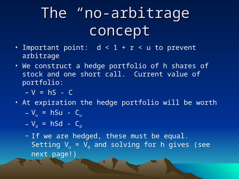
• Important point: d < 1 + r < u to prevent arbitrage• We construct a hedge portfolio of h shares of stock and

one short call. Current value of portfolio:– V = hS - C

• At expiration the hedge portfolio will be worth

– Vu = hSu - Cu

– Vd = hSd - Cd

– If we are hedged, these must be equal. Setting Vu = Vd and solving for h gives (see next page!)

One-Period Binomial Model One-Period Binomial Model (continued)(continued)

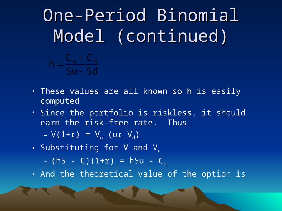
• These values are all known so h is easily computed• Since the portfolio is riskless, it should earn the risk-

free rate. Thus

– V(1+r) = Vu (or Vd)

• Substituting for V and Vu

– (hS - C)(1+r) = hSu - Cu

• And the theoretical value of the option is

SdSu

CCh du

No-arbitrage conditionNo-arbitrage condition

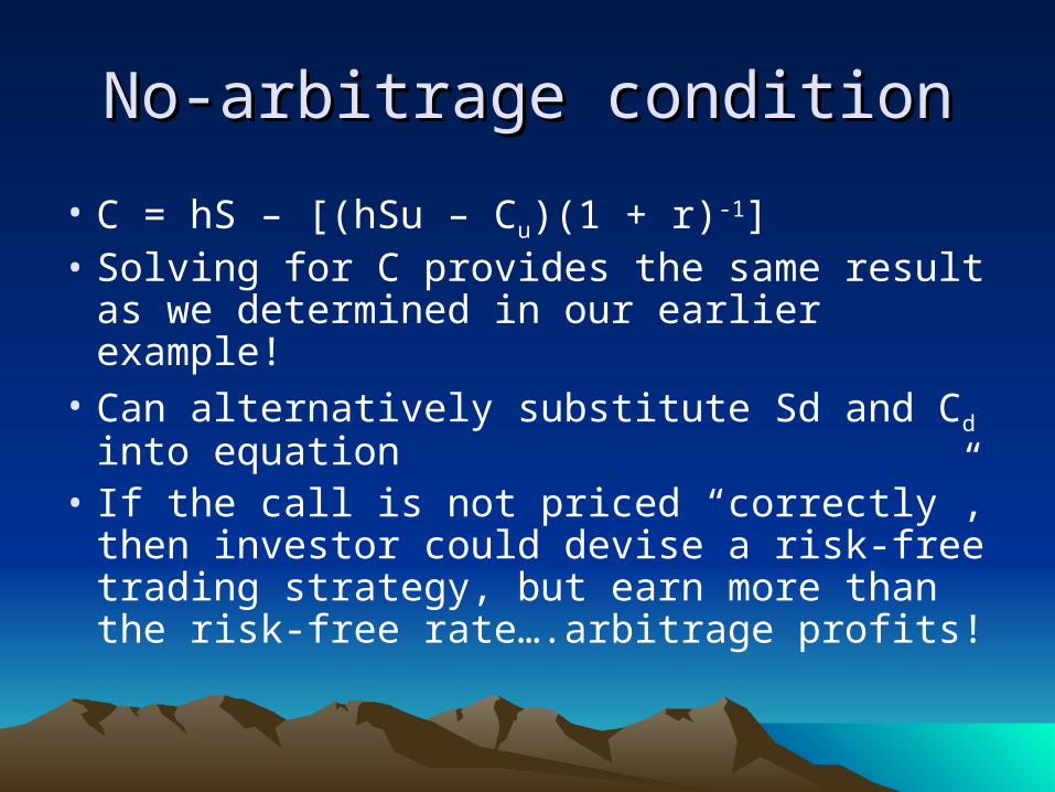
• C = hS – [(hSu – Cu)(1 + r)-1]• Solving for C provides the same result as

we determined in our earlier example!• Can alternatively substitute Sd and Cd into

equation• If the call is not priced “correctly”, then

investor could devise a risk-free trading strategy, but earn more than the risk-free rate….arbitrage profits!

One-Period Binomial Model risk-free One-Period Binomial Model risk-free portfolio exampleportfolio example

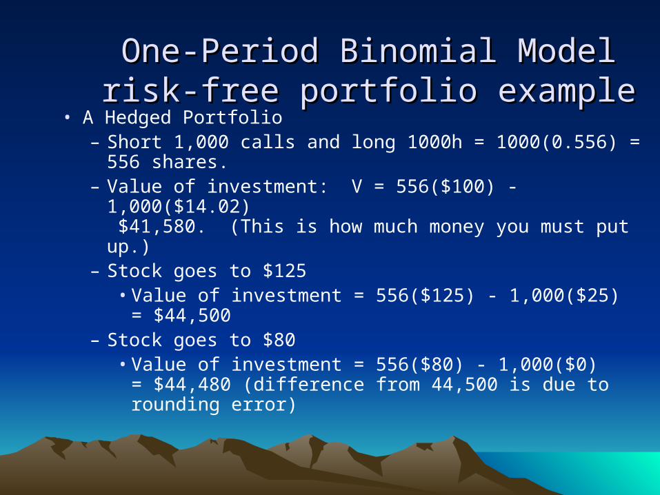
• A Hedged Portfolio – Short 1,000 calls and long 1000h = 1000(0.556) = 556

shares.– Value of investment: V = 556($100) - 1,000($14.02)

$41,580. (This is how much money you must put up.)– Stock goes to $125

• Value of investment = 556($125) - 1,000($25) = $44,500

– Stock goes to $80• Value of investment = 556($80) - 1,000($0)

= $44,480 (difference from 44,500 is due to rounding error)

One-Period Binomial Model (continued)One-Period Binomial Model (continued)

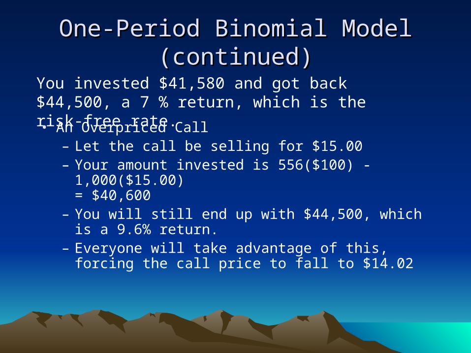
• An Overpriced Call– Let the call be selling for $15.00– Your amount invested is 556($100) - 1,000($15.00)

= $40,600– You will still end up with $44,500, which is a 9.6%

return.– Everyone will take advantage of this, forcing the call

price to fall to $14.02

You invested $41,580 and got back $44,500, a 7 % return, which is the risk-free rate.

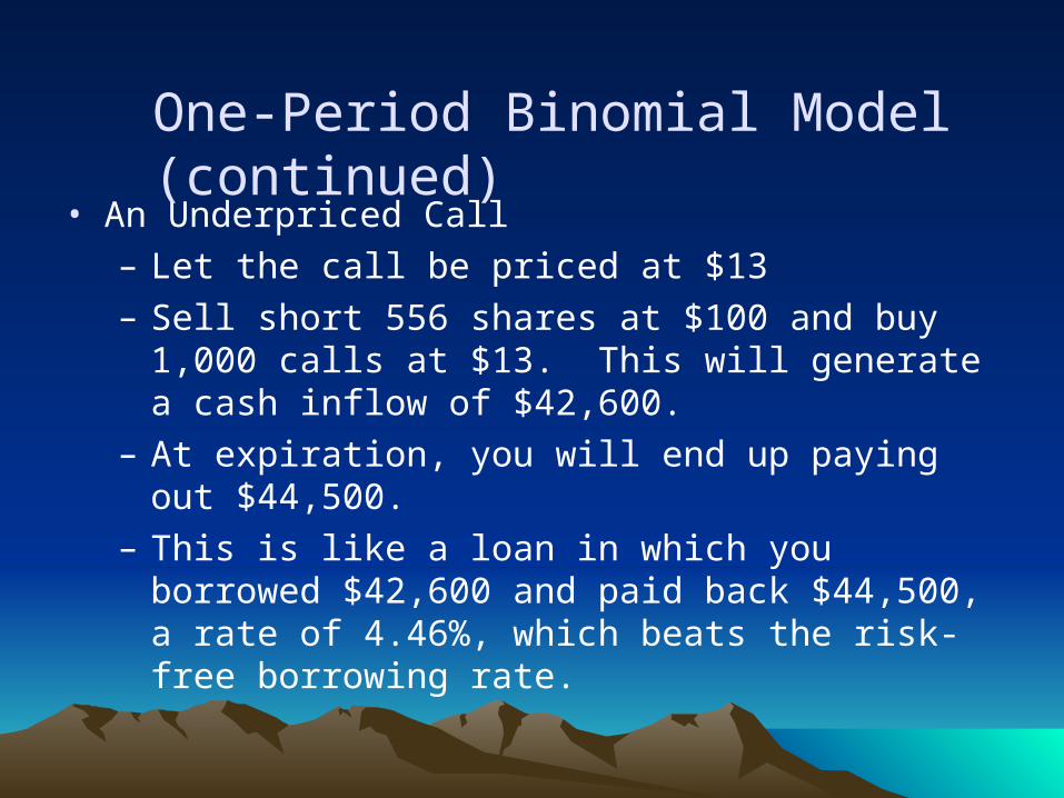
• An Underpriced Call– Let the call be priced at $13– Sell short 556 shares at $100 and buy 1,000 calls at

$13. This will generate a cash inflow of $42,600.– At expiration, you will end up paying out $44,500.– This is like a loan in which you borrowed $42,600 and

paid back $44,500, a rate of 4.46%, which beats the risk-free borrowing rate.

One-Period Binomial Model (continued)

Two-Period Binomial Model risk-free Two-Period Binomial Model risk-free portfolio exampleportfolio example

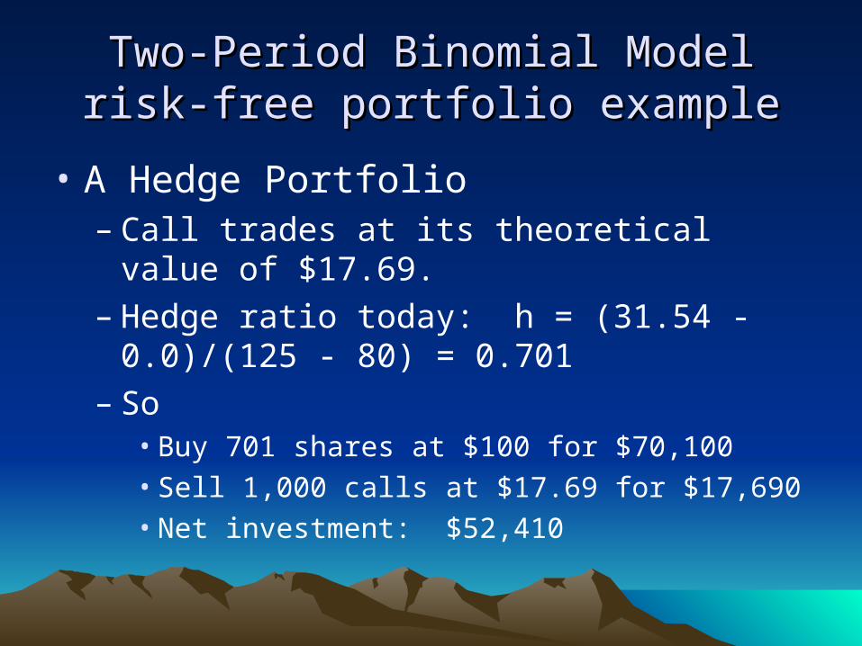
• A Hedge Portfolio– Call trades at its theoretical value of $17.69.– Hedge ratio today: h = (31.54 - 0.0)/(125 - 80)

= 0.701– So

• Buy 701 shares at $100 for $70,100• Sell 1,000 calls at $17.69 for $17,690• Net investment: $52,410

Two-Period Binomial Model (continued)Two-Period Binomial Model (continued)

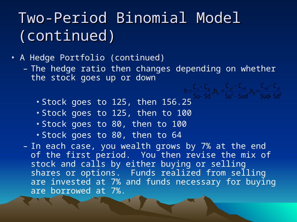
• A Hedge Portfolio (continued)– The hedge ratio then changes depending on whether the

stock goes up or down

• Stock goes to 125, then 156.25• Stock goes to 125, then to 100• Stock goes to 80, then to 100• Stock goes to 80, then to 64

– In each case, you wealth grows by 7% at the end of the first period. You then revise the mix of stock and calls by either buying or selling shares or options. Funds realized from selling are invested at 7% and funds necessary for buying are borrowed at 7%.

2dud

d2

uduu

du

SdSud

CCh ,

SudSu

CCh ,

SdSu

CCh

22

Two-Period Binomial Model Two-Period Binomial Model (continued)(continued)

• A Hedge Portfolio (continued)– Your wealth then grows by 7% from the end

of the first period to the end of the second.– Conclusion: If the option is correctly priced

and you maintain the appropriate mix of shares and calls as indicated by the hedge ratio, you earn a risk-free return over both periods.

Two-Period Binomial Model Two-Period Binomial Model (continued)(continued)

• A Mispriced Call in the Two-Period World– If the call is underpriced, you buy it and short

the stock, maintaining the correct hedge over both periods. You end up borrowing at less than the risk-free rate.

– If the call is overpriced, you sell it and buy the stock, maintaining the correct hedge over both periods. You end up lending at more than the risk-free rate.

Extensions of the binomial modelExtensions of the binomial model

• Early exercise (American options)

• Put options

• Call options with dividends

• Real option examples

Pricing Put OptionsPricing Put Options

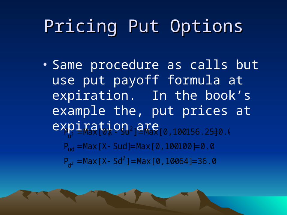
• Same procedure as calls but use put payoff formula at expiration. In the book’s example the, put prices at expiration are

36.064]Max[0,100]SdMax[XP

0.0100]Max[0,100Sud]Max[XP

0.0156.25]Max[0,100]SuXMax[0,P

2d

ud

2u

2

2

Pricing Put Options (continued)Pricing Put Options (continued)

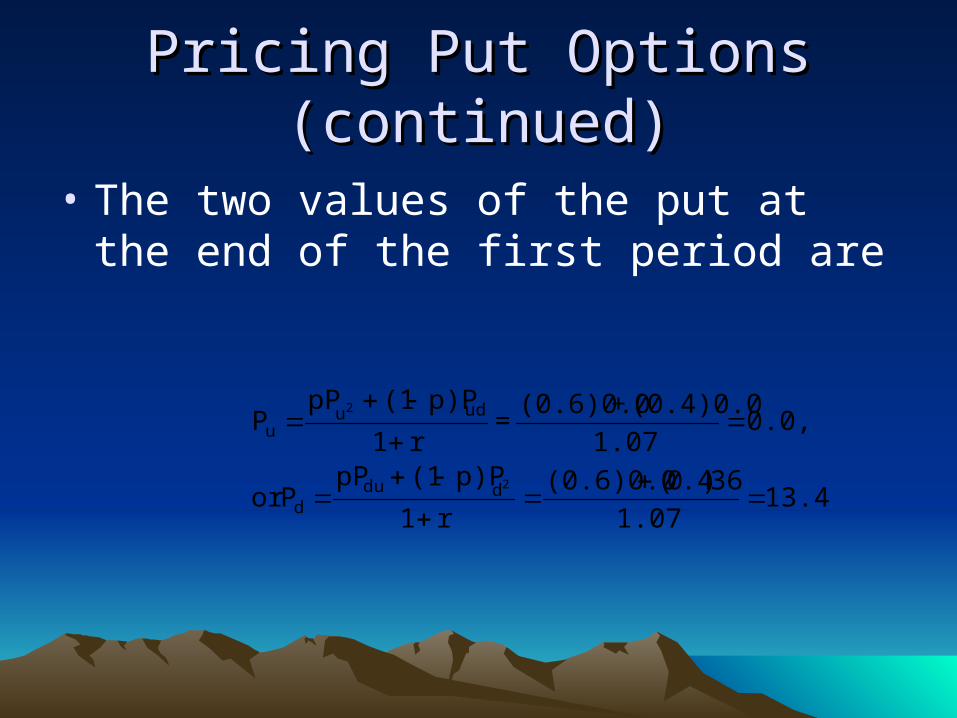
• The two values of the put at the end of the first period are

13.461.07

36).40((0.6)0.0

r1

p)P(1pPPor

0.0,1.07

(0.4)0.0+(0.6)0.0=

r1

p)P(1pPP

2

2

ddud

uduu

Pricing Put Options (continued)Pricing Put Options (continued)

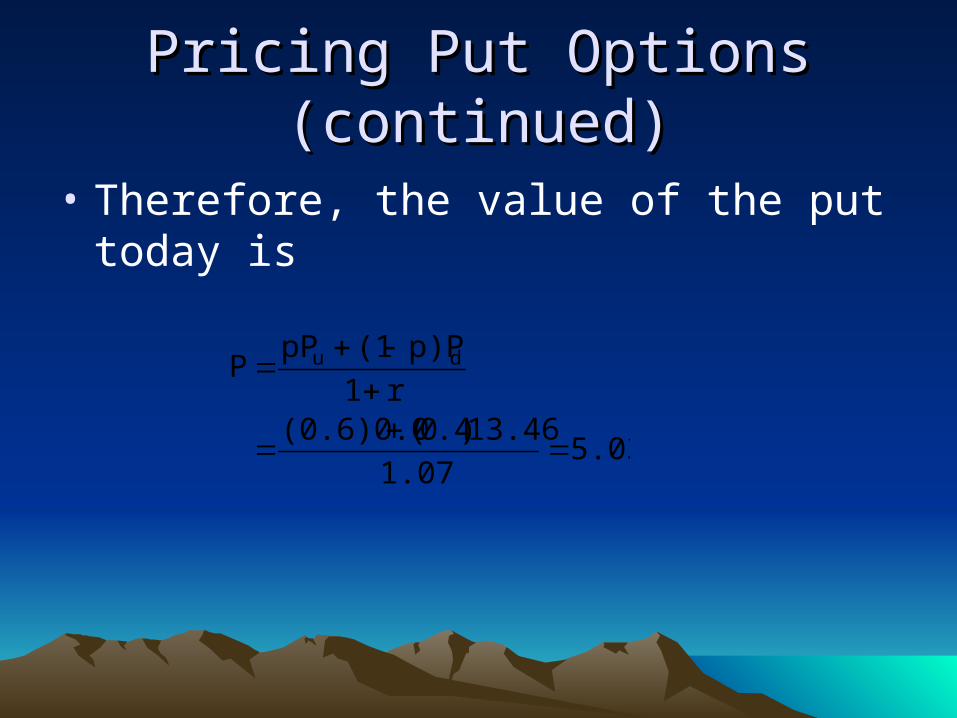
• Therefore, the value of the put today is

5.031.07

13.46).40((0.6)0.0r1

p)P(1pPP du

Pricing Put Options (continued)Pricing Put Options (continued)

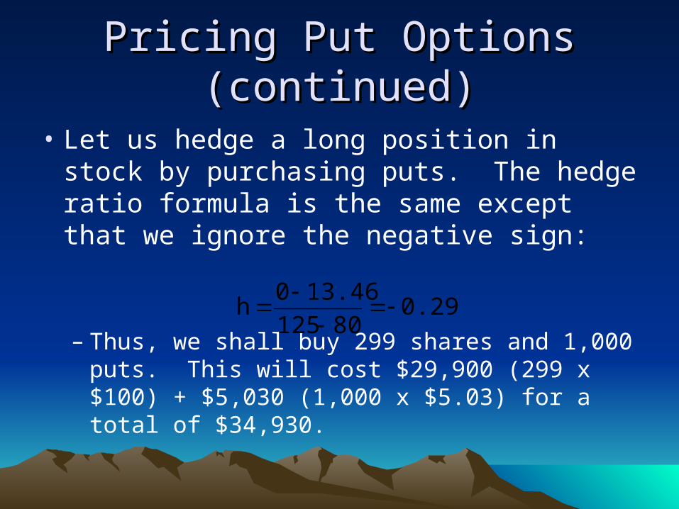
• Let us hedge a long position in stock by purchasing puts. The hedge ratio formula is the same except that we ignore the negative sign:

– Thus, we shall buy 299 shares and 1,000 puts. This will cost $29,900 (299 x $100) + $5,030 (1,000 x $5.03) for a total of $34,930.

0.29980125

13.460h

Pricing Put Options (continued)Pricing Put Options (continued)

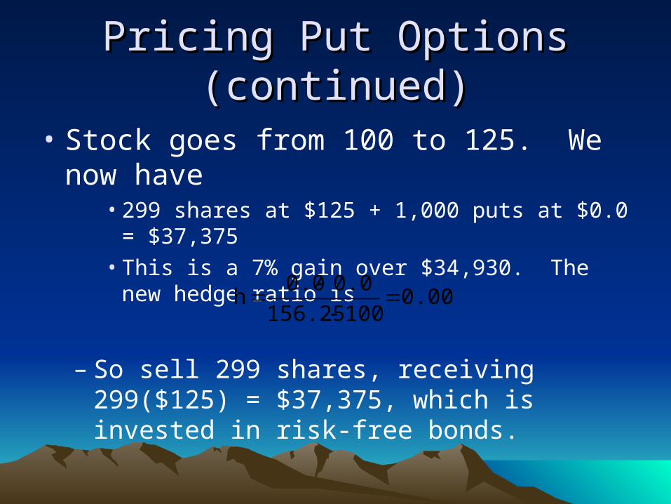
• Stock goes from 100 to 125. We now have

• 299 shares at $125 + 1,000 puts at $0.0 = $37,375• This is a 7% gain over $34,930. The new hedge

ratio is

– So sell 299 shares, receiving 299($125) = $37,375, which is invested in risk-free bonds.

0.000100156.25

0.00.0h

Pricing Put Options (continued)Pricing Put Options (continued)

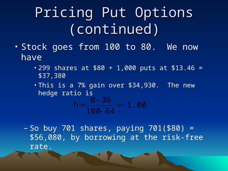
• Stock goes from 100 to 80. We now have• 299 shares at $80 + 1,000 puts at $13.46 =

$37,380• This is a 7% gain over $34,930. The new hedge

ratio is

– So buy 701 shares, paying 701($80) = $56,080, by borrowing at the risk-free rate.

1.00064100

360h

Pricing Put Options (continued)Pricing Put Options (continued)

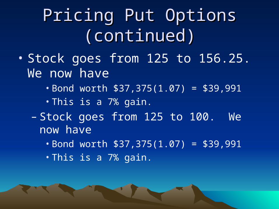
• Stock goes from 125 to 156.25. We now have

• Bond worth $37,375(1.07) = $39,991• This is a 7% gain.

– Stock goes from 125 to 100. We now have• Bond worth $37,375(1.07) = $39,991• This is a 7% gain.

Pricing Put Options (continued)Pricing Put Options (continued)

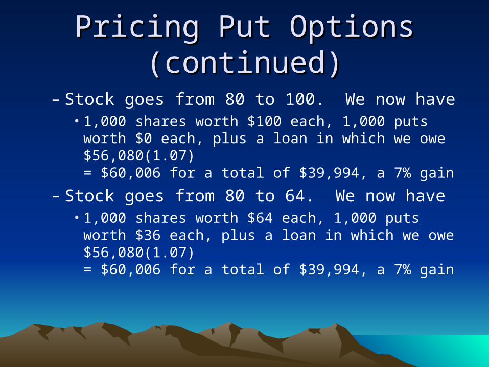
– Stock goes from 80 to 100. We now have• 1,000 shares worth $100 each, 1,000 puts worth

$0 each, plus a loan in which we owe $56,080(1.07) = $60,006 for a total of $39,994, a 7% gain

– Stock goes from 80 to 64. We now have• 1,000 shares worth $64 each, 1,000 puts worth

$36 each, plus a loan in which we owe $56,080(1.07) = $60,006 for a total of $39,994, a 7% gain

Early Exercise & American PutsEarly Exercise & American Puts

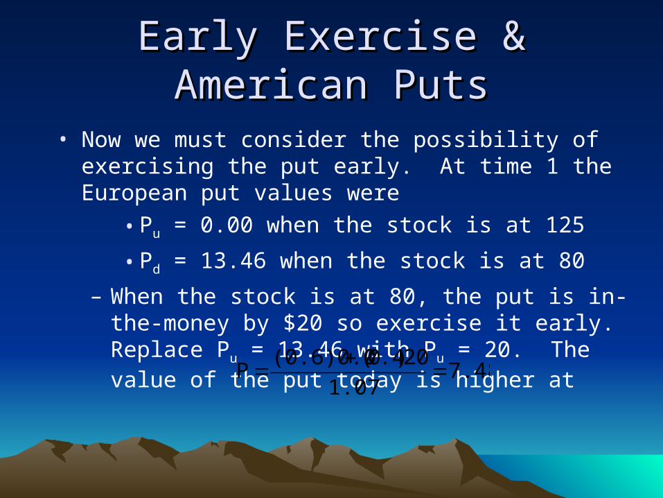
• Now we must consider the possibility of exercising the put early. At time 1 the European put values were

• Pu = 0.00 when the stock is at 125

• Pd = 13.46 when the stock is at 80

– When the stock is at 80, the put is in-the-money by $20 so exercise it early. Replace Pu = 13.46 with Pu = 20. The value of the put today is higher at

7.481.07

20).40((0.6)0.0P

Call options and dividendsCall options and dividends

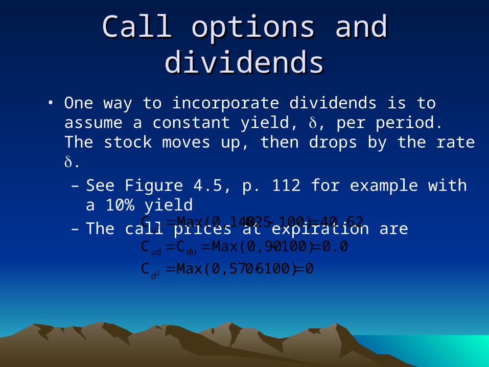
• One way to incorporate dividends is to assume a constant yield, , per period. The stock moves up, then drops by the rate .– See Figure 4.5, p. 112 for example with a 10% yield– The call prices at expiration are

0100)0Max(0,57.6C

0.0100)Max(0,90CC

40.625100)625Max(0,140.C

2

2

d

duud

u

Calls and dividends (continued)Calls and dividends (continued)

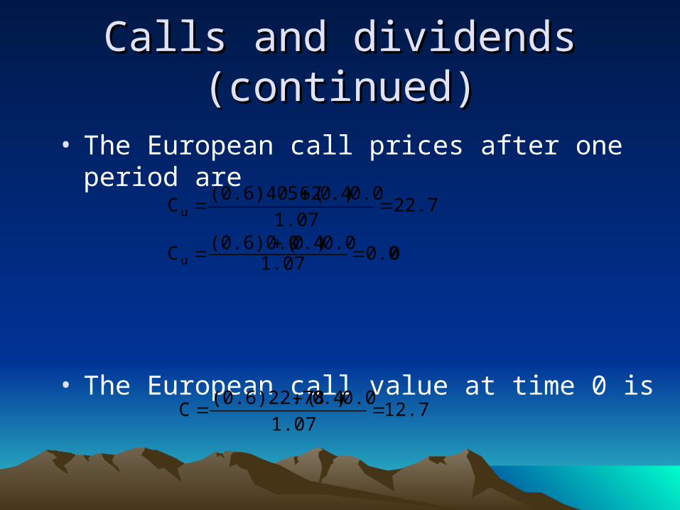
• The European call prices after one period are

• The European call value at time 0 is

00.01.070.0).40( (0.6)0.0

C

22.781.07

0.0).40(5(0.6)40.62C

u

u

12.771.07

0.0).40((0.6)22.78C

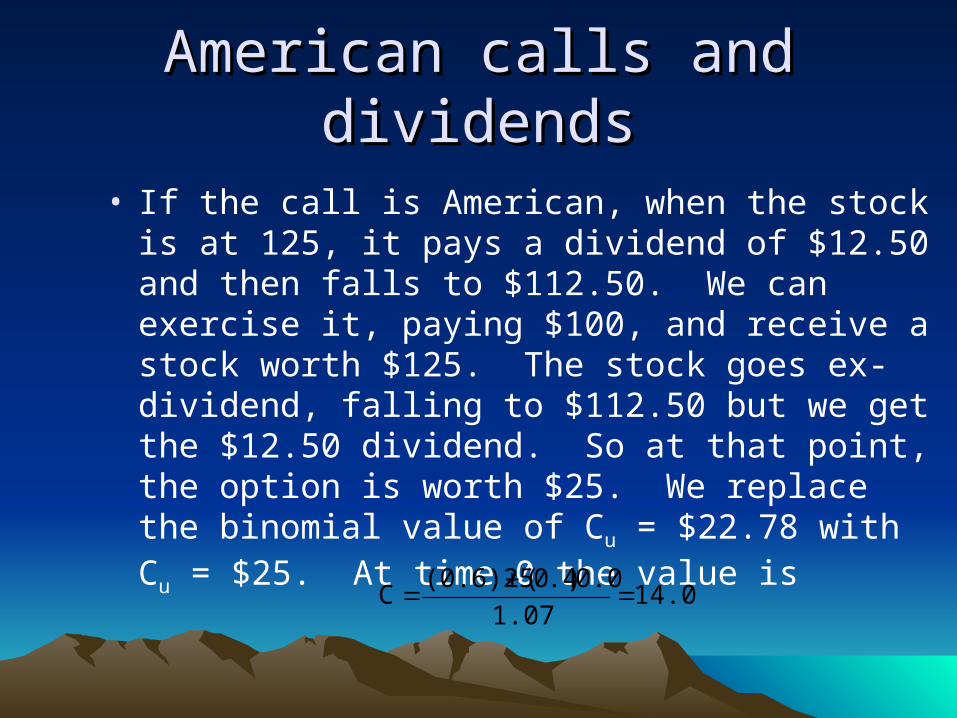
American calls and dividendsAmerican calls and dividends

• If the call is American, when the stock is at 125, it pays a dividend of $12.50 and then falls to $112.50. We can exercise it, paying $100, and receive a stock worth $125. The stock goes ex-dividend, falling to $112.50 but we get the $12.50 dividend. So at that point, the option is worth $25. We replace the binomial value of Cu = $22.78 with Cu = $25. At time 0 the value is

14.021.07

0.0).40((0.6)25C

Calls and dividendsCalls and dividends

• Alternatively, we can specify that the stock pays a specific dollar dividend at time 1. Assume $12. Unfortunately, the tree no longer recombines, as in Figure 4.6, p. 113. We can still calculate the option value but the tree grows large very fast. See Figure 4.7, p. 114.

• Because of the reduction in the number of computations, trees that recombine are preferred over trees that do not recombine.

Calls and dividendsCalls and dividends

• Yet another alternative (and preferred) specification is to subtract the present value of the dividends from the stock price (as we did in Chapter 3) and let the adjusted stock price follow the binomial up and down factors. For this problem, see Figure 4.8, p. 115.

• The tree now recombines and we can easily calculate the option values following the same procedure as before.

Real optionsReal options

• An application of binomial option valuation methodology to corporate financial decision making.

• Consider an oil exploration company– Traditional NPV analysis assumes that decision to

operate is “binding” through the life of the project.– Real options analysis adds “flexibility” by allowing

management to consider abandonment of project if oil prices drop too low.

– If “option” adds value to the project, then Project value = NPV of project + value of real options

– See spreadsheet example.

Next full week of class (sessions 11 Next full week of class (sessions 11 & 12)& 12)

• Black-Scholes model– Assumptions– Valuation equation– “Greeks”– Extensions

• Put option• Incorporating dividends

– Implied volatility