DBA*

A Real-Time Path Finding Algorithm

By

William Lee

A Thesis Submitted in Partial Fulfillment of the Requirements for the Degree of

Bachelor of Arts Honours

In

The Irving K. Barber School of Arts and Sciences

(Honors Computer Science Major Computer Science)

The University of British Columbia

(Okanagan)

April 2013

© William Lee, 2013

Abstract

Grid-based path finding is required in many video games and virtual worlds to move agents.

With both map sizes and the number of agents increasing, it is important to develop path

finding algorithms that are efficient in memory and time. In this work, we present an algorithm

called DBA* that uses a database of pre-computed paths to reduce the time to solve search

problems. When evaluated using benchmark maps from Dragon AgeTM, DBA* requires less

memory and time for search, and performs less pre-computation than comparable real-time

search algorithms. Further, its sub optimality is less than 3%, which is better than the PRA*

implementation used in Dragon AgeTM.

Table of Contents

Abstract................................................................................................................................ 2

Table of Contents ................................................................................................................ 3

1 Introduction….................................................................................................................... 6

1.1 Motivation……………........................................................................................................ 6

1.2 Goals and Objectives....................................................................................................... 6

1.3 Thesis Statement and Contributions............................................................................... 7

2 Background........................................................................................................................ 8

2.1 A*……………...................................................................................................................... 8

2.2 PRA*…………….................................................................................................................. 8

2.3 TBA*…………….................................................................................................................. 9

2.4 LRTA*……………................................................................................................................ 9

2.5 D LRTA*……………............................................................................................................. 10

2.6 KNN LRTA*……………........................................................................................................ 10

2.7 HCDPS……………................................................................................................................ 10

2.8 Summary……………........................................................................................................... 10

3 Approach Overview........................................................................................................... 12

4 Implementation Example ................................................................................................. 14

4.1 Offline Abstraction……………............................................................................................ 14

4.2 Offline Database Generation.......................................................................................... 15

4.3 Online Pathfinding……….................................................................................................. 16

4.4 Optimization……….……….................................................................................................. 16

4.5 Path Trimming…….……….................................................................................................. 17

4.6 Increasing Neighborhood Depth..................................................................................... 17

5 Experimental Results......................................................................................................... 19

5.1 Online Performance…………….......................................................................................... 19

5.2 Precomputation……….................................................................................................... 21

5.3 Scalability…………………….………........................................................................................ 21

5.4 Scalability of Online Performance.……........................................................................... 22

5.5 Scalability of Offline Precomputation………..................................................................... 22

6 Conclusion......................................................................................................................... 25

7 Future Work...................................................................................................................... 25

Appendix A……...................................................................................................................... 26

References……...................................................................................................................... 27

Table of Figures

Figure 1: Regions and Sector Abstraction Example.............................................................. 14

Figure 2: Path Matrix for Example Map………………………………………....................................... 15

Figure 3: Online Path Finding Example................................................................................. 16

Figure 4: Path Trimming Reduces Suboptimality When Combining Path Fragments......... 17

Figure 5: Solution Path when Database Stores Paths

Between Regions Up to 2 Regions Away……………………………………………….. 18

Figure 6: Suboptimality versus Move Time (DAO)…….......................................................... 20

Figure 7: Suboptimality versus Total Memory Used (DAO).................................................. 20

Figure 8: Database Generation Time versus Database Generation Size (DAO).................... 21

Figure 9: Aggregated Suboptimality versus Move Time (DAO)….......................................... 22

Figure 10: Aggregated Suboptimality versus Move Time (CSS)……....................................... 22

Figure 11: Aggregated Suboptimality versus Memory Use (DOA)........................................ 23

Figure 12: Aggregated Suboptimality versus Memory Use (CSS)..........................................23

Figure 13: Aggregated DB Generation time vs DB size (DOA)……......................................... 24

Figure 14: Aggregated DB Generation time vs DB size (CSS)................................................ 24

1 Introduction

As games have evolved, their size and complexity has increased. The virtual worlds and maps

have become larger as have the number of agents interacting. It is not uncommon for hundreds

of agents to be path finding simultaneously, yet the processing time dedicated to path finding

has not substantially increased. Consequently, game developers are often forced to make

compromises on path finding algorithms and spend considerable time tuning and validating

algorithm implementations. Variations of A* and PRA* are commonly used in video games [9].

The limitation of these algorithms is that they must plan a complete (but possibly abstract) path

before the agent can move. Real-time algorithms such as kNN LRTA* [3] and HCDPS [8]

guarantee a constant bound on planning time, but these algorithms often require a

considerable amount of pre-computation time and space. In this work, we propose a grid-based

path finding algorithm called DBA* that combines the real-time constant bound on planning

time enabled by using a pre-computed database as in HCDPS [8] with abstraction using sectors

as used in PRA* [9]. The result is a path finding algorithm that uses less space than previous

real-time algorithms while providing better paths than PRA* [9]. DBA* was evaluated on

Dragon AgeTMmaps from [10] with average suboptimality less than 3% and requiring on

average less than 200 KB of memory and between 1 and 10 seconds for pre-computation.

1.1 Motivation

To improve upon existing real time path finding algorithms for grid space search. Current state

of the art real time path finding algorithms are all trading off important aspects of an algorithm

in order to guarantee a constant bound on response time. All existing solutions make

substantial sacrifices in respect to suboptimality, pre-computation time, or memory usage,

sometimes on all fronts. Minimizing penalties on any aspects will have tangible benefits in this

field. Real time path finding also needs to redo most, if not all pre-computation when there are

changes to the map. Gracefully handling dynamic map updates will be a significant

achievement.

1.2 Goals and Objectives

The primary goal of this thesis is to write a new algorithm that outperforms existing state-of-

the-art algorithms for grid-based path finding. A secondary goal is to investigate how to handle

a dynamically changing map more gracefully than existing algorithms.

1.3 Thesis Statement and Contributions

The contribution of this thesis is the development of a new real time path finding algorithm,

DBA*, which combines the best features of two previous state of the art real time path finding

algorithms. DBA* is in line with the other algorithms in terms of memory usage, and it

outperforms others on measures such as path quality and response time.

2 Background

This work formulates grid-based path finding as a heuristic search problem where states are

vacant square grid cells. Each cell is connected to four cardinally (i.e., N, E, W, S) and four

diagonally neighboring cells. Out-edges of a vertex are moves available in the cell. The edge

costs are 1 for cardinal moves and 1.4 for diagonal moves. Standard octile distance is used for

the heuristic. The algorithm studied in this paper, although potentially adaptable to general

heuristic search, is specifically designed and optimized for 2D grid-based path finding.

Algorithms are evaluated based on the quality of the path produced and the amount of

time and memory resources consumed. Suboptimality is defined as the ratio of the path cost

found by the agent to the optimal solution cost minus one and times 100%. Sub optimality of

0% indicates an optimal path and sub optimality of 50% indicates a path 1.5 times as costly as

the optimal path.

An algorithm is also characterized by its response time, which is the maximum planning

time per move. The overall time is the total amount of time to construct the full solution, and

the average move time is the overall time divided by the number of moves made. Memory is

consumed for node expansions (e.g. open and closed lists in A*), for storing abstraction

information (e.g. regions), and for storing computed paths. Per agent memory is memory

consumed for each search agent. Fixed memory is memory consumed that is shared across

multiple, concurrent path finding agents.

2.1 A*

A* [5] is a common algorithm used for video game path finding as it has good performance

characteristics and is straightforward to implement. The A* algorithm uses a heuristic to restrict

the number of states that must be evaluated before finding the true optimal path. It guarantees

to expand an equal number or fewer states than any other algorithm using the same heuristic.

A* paths are always optimal as long as the heuristic function is admissible; that is, it never

overestimates the distance to the goal. However A* must plan a full path before the first move

can be made. Thus its response is equivalent to the overall time required to find a complete

solution which depends on the problem size and complexity. This can result in highly variable

times and in the worst case, A* may be too slow. Its memory use is also variable and may be

high depending on the size of its open and closed lists and the heuristic function used.

2.2 PRA*

The PRA* variant implemented in Dragon Age [9] was designed to improve on A* performance

for path finding. PRA* response time and per agent memory are reduced by abstracting the

search space into sectors and first computing a complete solution in the abstract space. Sub

sections of the solution are then refined using A*. The abstraction reduces the size of the

problem to be solved but requires a small amount of fixed memory. It also results in solutions

that are suboptimal. Even with path refinement, suboptimality has been reported to be

between 5 to 15%. The small trade-off in space and sub optimality is beneficial for faster

response time.

Real-time Algorithms

In situations when a solution is required in a fixed amount of time, traditional algorithms such

as A* may not be fast enough. For such situations, real time algorithms may be used instead. A

real-time algorithm differs from a traditional algorithm in the sense that regardless of state

space size, the agent per move planning time is bounded. Such algorithms often rely on some

form of pre-computation to speed up the path finding process. Some loss in quality is usually

observed amongst solutions found by real-time algorithms.

2.3 TBA*

TBA* [1] is a time-sliced version of A* that exhibits the same properties as A* with the added

ability to control response time and per move planning time. TBA* works by interleaving

planning and moving. It starts off expanding stats the same way A* does. Once a given number

of states is expanded, TBA* interrupts the planning phase and starts a back tracing process to

find the original start state until the agent is found. Once the agent is found, the agent’s next

action is simply to follow the new path created by back tracing. If the agent ever ends up in a

situation where it has no path to follow, the agent will back track towards the start state. TBA*

is a complete algorithm in the sense that it guarantees that the agent will eventually get on the

solution path if one exists. However, units may have to repeatedly back track all the way to the

start in some cases. Unlike other algorithms, TBA* does not rely on some form of pre-

computation to speed up online search, nor does it require state space abstraction. However, it

does require extensive re-planning in the worst case.

2.4 LRTA*

LRTA* with subgoals [6] pre-computes a subgoal tree from each goal state where a subgoal is

the next target state to exit a heuristic depression. Online, LRTA* will be able to use the subgoal

tree to escape a heuristic depression. It is also possible to compute a solution to the all-pairs

shortest path problem and store it in a compressed form. Algorithms such as [2] store for each

pair of states the next direction or state to visit along an optimal path. Depending on the

compression, it is possible to achieve perfect solutions at run-time very quickly with the

compromise of considerable pre-computation time and space to store the compressed

databases.

2.5 D LRTA*

D LRTA* [4] performs clique abstraction and generates next hop information between regions

allowing an agent to know the next region to traverse to. D LRTA* attempts to remove learning

from classical LRTA* by automatically selecting subgoals. The size of the abstraction and its pre-

computation time were significant.

2.6 KNN LRTA*

kNN LRTA* [3] created a database of compressed problems and online used the closest

problem in the database as a solution template. It is an improved version of D LRTA* which has

been reported to use approximately nine times less memory and only suffers a small loss in

path quality compared to D LRTA*. Database construction time is however still an issue, and

there is no guarantee of complete coverage. Another major weakness with these two

algorithms is that they fall back on LRTA* when no information is in the database, which may

result in very suboptimal solutions.

2.7 HCDPS

HCDPS *8+ performs offline abstraction by defining regions where all states are bi-directionally

hill-climbable with the region representative. A compressed path database was then

constructed defining paths between all region representatives. This allows all searches to be

done using hill-climbing, which results in minimal per agent memory use. HCDPS is faster than

PRA* with improved path suboptimality, but its abstraction consumes more memory.

2.8 Summary

All of these algorithm implementations balance search time versus memory used. The “best”

algorithm depends on the video game path finding environment and its requirements. There

are three properties that algorithms should have to be useful in practice:

- Solution consistency - The quality of the solutions (suboptimality) should not vary

dramatically between problems.

- Adequate response time - The hard-limits on the response time dictated by the game

must be met.

- Memory efficiency - The amount of per agent memory and fixed memory should be

minimized.

The goal is to minimize suboptimality, response time, and memory usage.

3 Approach Overview

This work combines and extends the best features of two previous algorithms to improve these

metrics. Specifically, the memory-efficient sector abstraction developed for *9+ is integrated

with the path database used by HCDPS [8] to improve suboptimality, memory usage, and

response time. The DBA* algorithm performs offline pre-computation before online path

finding. The offline stage abstracts the grid into sectors and regions and pre-computes a

database of paths to navigate between adjacent regions. A sector is a grid of cells (e.g. 16

x 16). The sector number for a cell ( , ) is calculated by

⌊

⌋ ⌊

⌋ ⌊

⌋

(1)

where is the width of the grid map. A region is a set of cells in a sector that are mutually

reachable without leaving the sector. Regions are produced by performing one or more

breadth-first searches until all cells in a sector are assigned to a region. A sector may have

multiple regions, and a region is always in only one sector. A region center or representative

state is selected for each region. The definition and construction of regions follows that in *9+.

DBA* then proceeds to construct a database of optimal paths between the

representatives of adjacent regions using A*. Each path found is stored in compressed format

by storing a sequence of subgoals, each of which can be reached from the previous subgoal via

hill-climbing. Hill-climbing compressible paths are described in [8].

To navigate between non-adjacent regions, a matrix (where is the number of

regions) is constructed where cell ( , ) contains the next region to visit on a path from to ,

the cost of that path, and the path itself (if the two regions are adjacent). The matrix is

initialized with the optimal paths between adjacent regions, and dynamic programming is

performed to determine the costs and next region to visit for all other matrix cells.

Online searches use the pre-computed database to reduce search time. Given a start

cell s and goal cell g, the sector for the start, , and for the goal, , are calculated using

Equation 1. If a sector only has one region, then the region is known immediately. Otherwise, a

BFS bounded within the sector is performed from s until it encounters some region

representative, . This is also performed for the goal state as well to find the goal region

representative, .

Given the start and goal region representatives, the path matrix is used to build a path

between and . This path may be directly stored in the database if the regions are

adjacent, or is the concatenation of paths by navigating through adjacent regions from

to . The complete path consists of navigating from to the region representative , then

following the subgoals to region representative , then navigating to . The response time is

almost immediate as the agent can start navigating from to the start region representative

as soon as the BFS is completed. The complete path between regions can be done iteratively

with the agent following the subgoals in a path from one region to the next without having to

construct the entire path. The overall time and number of states expanded are reduced as the

only search performed is the BFS to identify the start and goal regions if a sector contains

multiple regions.

4 Implementation Example

We describe the implementation using a running example.

4.1 Offline Abstraction

The first step in offline pre-computation is abstracting the search space into sectors as in [9].

Depending on the size of the map, the map is divided into fixed-sized sectors (e.g. 16 x 16 or 32

x 32). Note that there is no restriction that the sector sizes be square or a power of 2. Each

sector is divided into one or more regions using BFS. The sector size serves as an upper bound

for region size and limits the expansion of BFS during online path finding. If the sector size is

larger, BFS within the sector will take longer. If the sector size is small, the database will be

larger. In Figure 1 is a 6 sector subset of a map. The sector size is 16 x 16. Region

representatives are shown labeled with letters. Sector 5 (middle of bottom row) has two

regions E and F.

Fig. 1 Regions and Sector Abstraction Example

Region representatives are computed by summing the row (col) of each open state in the

region and then dividing by the number of open states. If this technique results in a state that is

a wall, adjacent cells are examined until an open state is found. DBA* and PRA* use this same

technique for region representative selection in the experiments. Other methods such as

proposed in [9] could also be used.

Unlike abstraction using cliques or hill-climbable regions, sector-based regions are built

in time where is the number of grid cells. Each state is expanded only once by a single

BFS. In comparison, the abstraction algorithm in HCDPS may expand a given state multiple

times.

The second major advantage is that the mapping between abstract state and base state

(i.e. what abstract region a given base state is in) does not need to be stored. Without

compression, this mapping consumes the same space as the map. Compression can reduce the

abstraction to about 10% of the map size [8]. Instead, to determine the region (and its region

representative) for a given cell, first the sector is calculated. If the sector has only one region,

then no search is required. Otherwise, a BFS is performed from the cell until it encounters one

of the region representative states listed for the sector. This BFS is bounded by the size of the

sector, and thus allows for a hard guarantee on the response time.

4.2 Offline Database Generation

After abstraction, a database of paths between adjacent region representatives are computed

using A* and stored in a path database. These paths are used to populate a path matrix

where is the total number of regions. Dynamic programming is performed on the matrix to

compute the cost and next hop region for all pairs of regions. Note that a complete path

between all pairs of regions is not stored. The path matrix only stores the cost and the next

region to traverse to. Paths are only stored between adjacent regions. This is very similar to

how a network routing table works where paths are outgoing links and a routing table stores

the address and cost of the next hop to route a message towards a given destination.

Fig. 2 Path Matrix for Example Map

As an example, in Figure 2 is the path matrix for the 6 sector map in Figure 1. Entries in

the matrix generated by dynamic programming are in italics. For example, the cost of a path

from A to C goes through B with a cost of 27.6.

4.3 Online Path Finding

Given a problem from start state to goal state , DBA* first determines the start region and

goal representatives and , using BFS if multiple regions are in the sector.

In Figure 3, the start state is in region E, and the goal state is in region G. Since sector 5

contains two regions, a BFS was required to identify region E. Region G was determined by

direct lookup as there was only one region in the sector.

Fig. 3 Online Path Finding Example

The minimal response time possible before the algorithm can make its first move is the time for

the BFS to identify the start region representative. At that point, the agent can navigate from

to using the path found during BFS.

The algorithm then looks in the path matrix to find the next hop to navigate from

to . In this case, that is to region B. As these are neighbor regions, a compressed path is

stored in the database, and the agent navigates using hill-climbing following its subgoals. Once

arriving at the representative for region B, it then goes to (representative of region G). If a

BFS path was computed to find that path can be used. Otherwise, DBA* completes the path

by performing A* bounded within the sector from to . The maximum move time is the first

response time for BFS. The maximum per agent memory is the number of states in a sector (as

may need to search entire sector with BFS).

4.4 Optimizations

Several optimizations were implemented to improve algorithm performance.

4.5 Path Trimming

The technique of path trimming was first described in PRA* [9] (remove last 10% of states in

each concatenated path and then plan from the end of the path to the next subgoal) and

extended in HCDPS (start and end optimizations). The general goal is to reduce the

suboptimality when concatenating smaller paths to produce a larger path. Combining several

smaller paths may produce longer paths with “bumps” compared to an optimal path. These

techniques smooth the paths to make them look more appealing and have lower suboptimality.

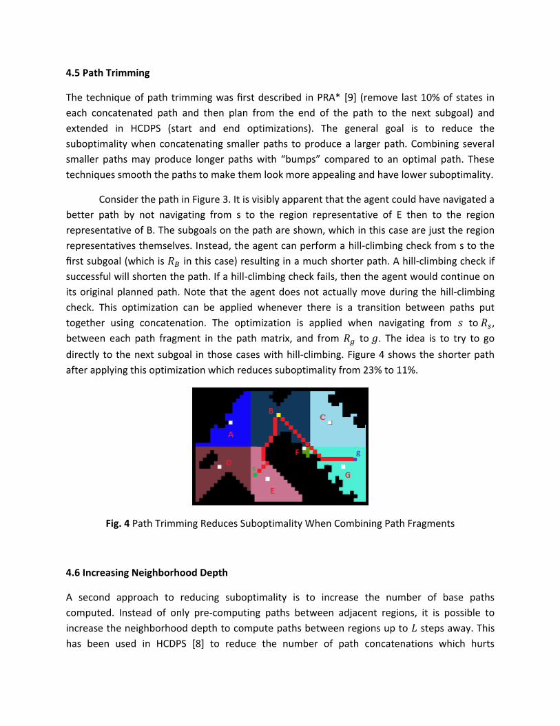
Consider the path in Figure 3. It is visibly apparent that the agent could have navigated a

better path by not navigating from s to the region representative of E then to the region

representative of B. The subgoals on the path are shown, which in this case are just the region

representatives themselves. Instead, the agent can perform a hill-climbing check from s to the

first subgoal (which is in this case) resulting in a much shorter path. A hill-climbing check if

successful will shorten the path. If a hill-climbing check fails, then the agent would continue on

its original planned path. Note that the agent does not actually move during the hill-climbing

check. This optimization can be applied whenever there is a transition between paths put

together using concatenation. The optimization is applied when navigating from to ,

between each path fragment in the path matrix, and from to . The idea is to try to go

directly to the next subgoal in those cases with hill-climbing. Figure 4 shows the shorter path

after applying this optimization which reduces suboptimality from 23% to 11%.

Fig. 4 Path Trimming Reduces Suboptimality When Combining Path Fragments

4.6 Increasing Neighborhood Depth

A second approach to reducing suboptimality is to increase the number of base paths

computed. Instead of only pre-computing paths between adjacent regions, it is possible to

increase the neighborhood depth to compute paths between regions up to steps away. This

has been used in HCDPS [8] to reduce the number of path concatenations which hurts

suboptimality. The tradeoff is a larger database size and longer pre-computation time. In the

running example, computing paths between regions up to 2 away results in a direct path

between region E and region G and reduces suboptimality for the example problem to 0%

(when used in combination with path trimming). Increasing neighborhood depth decreases

suboptimality but does not guarantee an optimal path.

Fig. 5 Solution Path when Database Stores Paths Between Regions Up to 2 Regions Away

5 Experimental Results

Algorithms were evaluated on ten of the largest standard benchmark maps from Dragon Age:

OriginsTM available at http://movingai.com and described in [10]. The 10 maps selected were

hrt000d, orz100d, orz103d, orz300d, orz700d, irz702, orz900d, ost000a, ost000t, and ost100d.

These maps have an average number of open states of 96,739 and total cells of 574,132. For

each map, 100 of the longest sample problems were run from the problem set.

The algorithms compared included DBA*, PRA* as implemented in Dragon Age [9], and

HCDPS. HCDPS was run for neighborhood depth = {1, 2, 3, 4}. PRA* was run for sector sizes of

16 x 16, 32 x 32, 64 x 64, and 128 x 128 and uses the 10% path trimming and re-planning

optimization. PRA* and DBA* both did not apply region center optimization, as region

representatives were computed by averaging the rows and columns of all open states in the

region. DBA* was run under all combinations of neighborhood level and grid size. LRTA* with

subgoals [7] was also evaluated. Algorithms were tested using Java 6 under SUSE Linux 10 on an

Intel Xeon E5620 2.4 GHz processor with 24 GB of memory.

In the charts, each point in the plot represents an algorithm with a different

configuration. For PRA*, there are 4 points corresponding to 16, 32, 64, and 128 sector sizes.

For HCDPS there are 4 points corresponding to levels 1, 2, 3, and 4. For DBA* that combines

both sets of parameters, there are separate series for each sector size (16, 32, 64, 128), and

each series consists of 4 points corresponding to levels 1, 2, 3, and 4.

5.1 Online Performance

Online performance consists of three factors: suboptimality of paths, total memory

used, and average move time. Figure 6 displays suboptimality versus move time. DBA* variants

(except for 128) are faster than HCDPS and PRA* and most variants have better suboptimality.

DBA* has the same or better suboptimality than HCDPS for smaller sector sizes. Larger sector

sizes for both DBA* and PRA* hurt suboptimality as the optimizations do not always counteract

navigating through region representatives that may be off an optimal path. Larger sector sizes

also dramatically increase the time for PRA* (PRA* 128 has 20 move time) as the amount of

abstraction is reduced and the algorithm is solving a problem using A* that is not much smaller

in the abstract space. Since DBA* uses its path database rather than solving using A* in the

abstract space, its move time does not increase as much with larger sectors. The additional

time is mostly related to the BFS required to find the region representatives in the start and

goal sectors. LRTA* with subgoals (shown as sgLRTA* in the legend) has different performance

characteristics than the other algorithms. sgLRTA* is almost optimal. Its move time is relatively

high because the subgoal trees are large, and it takes the algorithm time to identify the first

subgoal to use.

Fig. 6 Suboptimality versus Move Time (DAO)

Figure 7 compares suboptimality versus total memory used. PRA* uses less memory as

storing the regions and sectors requires minimal memory. The additional memory used by

DBA* to store paths between regions amounts to 50 to 250 KB, but improves suboptimality

from about 6% with PRA* to under 3%. DBA* dominates HCDPS in this metric. sgLRTA* is near

perfect for solution quality, but consumes significantly more memory to the point that it is not

practical in this domain.

Fig. 7 Suboptimality versus Total Memory Used (DAO)

For online performance, no algorithm dominates as each makes a different tradeoff on

time versus space. It is arguable that the improved path suboptimality and time of DBA* is a

reasonable tradeoff for the small amount of additional memory consumed. Unlike PRA*, DBA*

is optimized for static environments.

5.2 Pre-Computation

Pre-computation, although done offline, must also be considered in terms of time and memory

required. The results are in Figure 8. PRA* consumes the least amount of memory as it only

generates sectors and does not generate paths between sectors. HCDPS and DBA* both

perform abstraction and path generation, although DBA* in most configurations is faster with a

smaller database size. sgLRTA* that computes and compresses all paths takes considerably

longer and more space than all other algorithms.

Fig. 8 Database Generation Time versus Database Generation Size (DAO)

5.3 Scalability

In addition to testing on standard benchmark maps, DBA* is also tested on a set of 4 game

maps modeled after Counter-Strike: Source maps. These maps are magnified to having between

9 and 13 million states each. 1000 problems were randomly generated across the four maps

(250 each). We were interested in how DBA* performs in comparison to other approaches

especially in pre-computation for an exceptionally large search space. Our charts here show

average results because the visualization is otherwise too clustered and hard to comprehend.

SGLRTA* was also removed because it requires more memory for these problems than our

system can provide.

5.4 Scalability of Online Performance

Figure 9 shows the aggregated result of suboptimality vs. move time on DOA maps while Fig 10

shows aggregated result of suboptimality vs. move time on CSS map. As the map gets larger, all

three algorithm improved in both suboptimality and move time. This is a direct result from

being on a larger map. By enlarging the map and keeping the same sector size, the regions

become more fine-grained in relation to the map. This effect is similar to reducing sector size

for PRA* and DBA*. HCDPS does not benefit from this as directly because its region size is not

determined by a preset configuration but the size of hill-climbing reachable areas. Thus the

effect is on a different magnitude on HCDPS than on PRA* and DBA*.

Fig. 9 Aggregated Suboptimality versus Move Time (DAO)

Fig. 10 Aggregated Suboptimality versus Move Time (CSS)

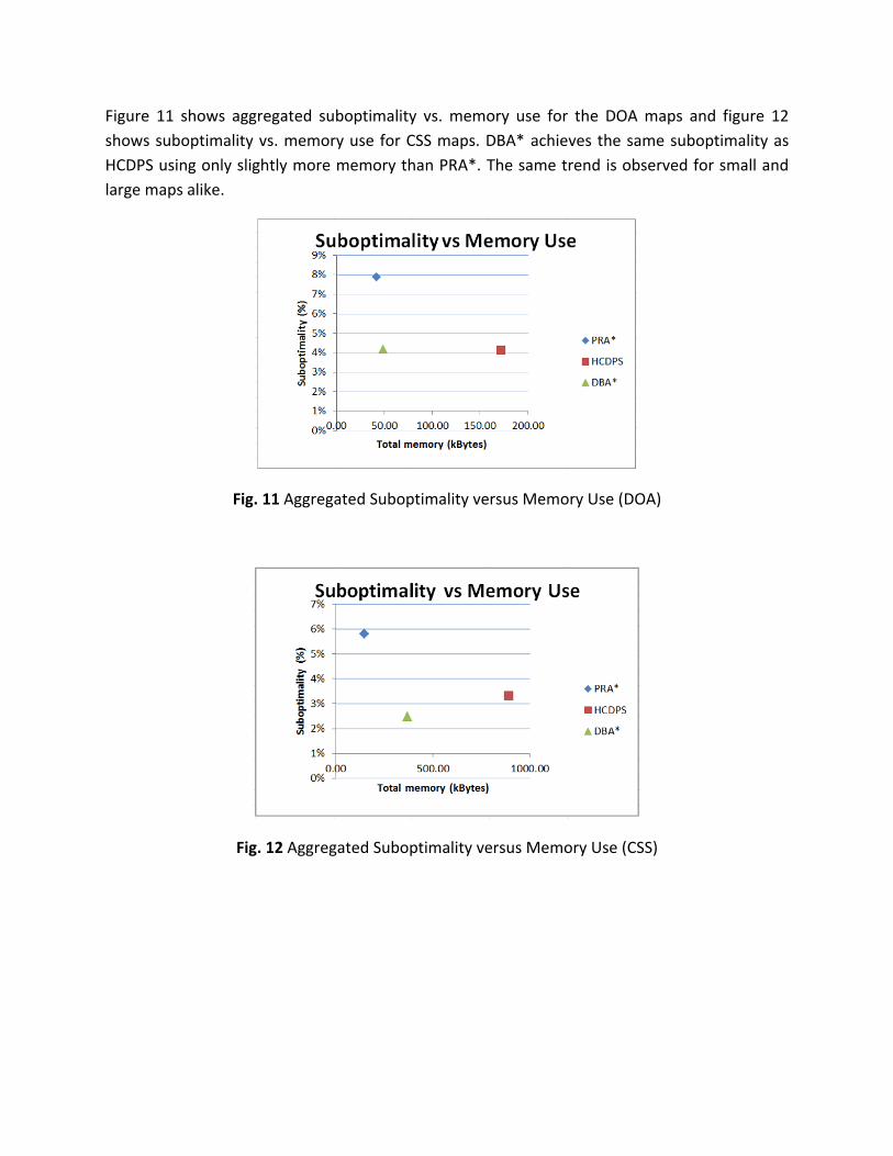
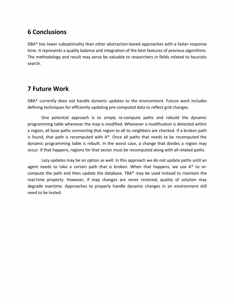
Figure 11 shows aggregated suboptimality vs. memory use for the DOA maps and figure 12

shows suboptimality vs. memory use for CSS maps. DBA* achieves the same suboptimality as

HCDPS using only slightly more memory than PRA*. The same trend is observed for small and

large maps alike.

Fig. 11 Aggregated Suboptimality versus Memory Use (DOA)

Fig. 12 Aggregated Suboptimality versus Memory Use (CSS)

5.5 Scalability of Offline Pre-Computation

Figure 13 shows database generation time vs. database size for DOA maps and Figure 14 shows

database generation time vs. database size for CSS maps. Because PRA* doesn’t store paths, it

will always be a clear winner in this measure. However, the pre-computation time required by

both HCDPS and DBA* are both reasonable given that this only has to be done once.

Fig. 13 Aggregated DB Generation time vs. DB size (DOA)

Fig. 14 Aggregated DB Generation time vs. DB size (CSS)

6 Conclusions

DBA* has lower suboptimality than other abstraction-based approaches with a faster response

time. It represents a quality balance and integration of the best features of previous algorithms.

The methodology and result may serve be valuable to researchers in fields related to heuristic

search.

7 Future Work

DBA* currently does not handle dynamic updates to the environment. Future work includes

defining techniques for efficiently updating pre-computed data to reflect grid changes.

One potential approach is to simply re-compute paths and rebuild the dynamic

programming table whenever the map is modified. Whenever a modification is detected within

a region, all base paths connecting that region to all its neighbors are checked. If a broken path

is found, that path is recomputed with A*. Once all paths that needs to be recomputed the

dynamic programming table is rebuilt. In the worst case, a change that divides a region may

occur. If that happens, regions for that sector must be recomputed along with all related paths.

Lazy updates may be an option as well. In this approach we do not update paths until an

agent needs to take a certain path that is broken. When that happens, we use A* to re-

compute the path and then update the database. TBA* may be used instead to maintain the

real-time property. However, if map changes are never restored, quality of solution may

degrade overtime. Approaches to properly handle dynamic changes in an environment still

need to be tested.

Appendix

A. Algorithm 1 Offline Database Generation // Compute optimal paths between adjacent regions using A*

for i = 0 to numRegions do

for j = 0 to numNeighbors of region[i] do

path = astar.computePath(region[i].center, region[j].center)

matrix[i][j].cost = cost of path

matrix[i][j].path = compress(path)

matrix[i][j].next = j

end for

end for

// Update matrix with dynamic programming

changed = true

while (changed) do

for i = 0 to numRegions do

for j = 0 to numNeighbors of region[i] do

for k = 0 to numRegions do

if (matrix[i][k].cost > matrix[i][j].cost+matrix[j][k].cost)then

matrix[i][k].cost = matrix[i][j].cost+matrix[j][k].cost

matrix[i][k].next = j

changed = true

end if

end for

end for

end for

end while

References

[1] Bjornsson, Y., Bulitko, V., Sturtevant, N.: TBA*: Time-bounded A*. In: Proceedings of the ¨International

Joint Conferences on Artificial Intelligence (IJCAI). pp. 431 – 436 (2009)

[2] Botea, A.: Ultra-fast optimal pathfinding without runtime search. In: Proceedings of the Second Artificial

Intelligence and Interactive Digital Entertainment Conference (AIIDE). pp. 122–127 (2011)

[3] Bulitko, V., Bjornsson, Y., Lawrence, R.: Case-based subgoaling in real-time heuristic search ¨for video

game pathfinding. Journal of Artificial Intelligence Research 39, 269–300 (2010)

[4] Bulitko, V., Lustrek, M., Schaeffer, J., Bj ˇ ornsson, Y., Sigmundarson, S.: Dynamic control in ¨real-time

heuristic search. Journal of Artificial Intelligence Research 32, 419 – 452 (2008)

[5] Hart, P., Nilsson, N., Raphael, B.: A formal basis for the heuristic determination of minimum cost paths.

IEEE Transactions on Systems Science and Cybernetics 4(2), 100–107 (1968)

[6] Hernandez, C., Baier, J.A.: Fast subgoaling for pathfinding via real-time search. In: Bacchus, ´F., Domshlak,

C., Edelkamp, S., Helmert, M. (eds.) Proceedings of the International Conference on Artificial Intelligence

Planning Systems (ICAPS). pp. 327–330. AAAI (2011)

[7] Hernandez, C., Baier, J.A.: Real-time heuristic search with depression avoidance. In: Proceedings of the

International Joint Conference on Artificial Intelligence (IJCAI). pp. 578–583 (2011)

[8] Lawrence, R., Bulitko, V.: Database-driven real-time heuristic search in video-game pathfinding. IEEE

Transactions on Computer Intelligence and AI in Games PP(99) (2013)

[9] Sturtevant, N.: Memory-efficient abstractions for pathfinding. In: Proceedings of Artificial Intelligence and

Interactive Digital Entertainment (AIIDE). pp. 31–36 (2007)

[10] Sturtevant, N.R.: Benchmarks for grid-based pathfinding. IEEE Transactions on Computer Intelligence and

AI in Games 4(2), 144–148 (2012)