Dead Lock Prevention And Hybrid Scheduling Algorithm
Zarwash Gulrez Khan, Marium Rehan
Abstract- the main focus of this research paper is the prevention and avoidance of deadlock. Multiple responsibilities and jobs like Input output, memory, and process and file management are the basic functionality of the operating System. A program of multiple instructions executed at run time is basically an operating and its most prioritized function is the management of processes. In a single processor system only on process can b executed at a time while the other process must wait for the CPU to be free and can be rescheduled. The objective of multi programming is the most effective way to provide multi tasking to maximize or increase the CPU utilization by running the process all the time. There are scheduling algorithms in abundance like FCFS, JSF, SRT, RR and a lot more for process scheduling. This report will evaluate and calculate these scheduling algorithms on the basis of their performance which include its 5 factors explained in the report, in a multi process surrounding and will propose or put forward a new hybrid schedule algorithm of preemptive and non preemptive nature as well as (HRRRN) known as “highest response round ratio next proposed by Brinch Hansen to avoid limitations of SJF algorithm” to find the best solution for CPU scheduling based on NOVEL algorithm and compare the performance of our hybrid scheduling algorithm to the previously created algorithms. The most vital objective the proposed algorithm is intended to do is increase the performance of CPU as compared to novel algorithm by minimizing waiting and turnaround time for a number of processes. Index Term: Scheduler, State Diagrams, CPU-Scheduling, Performance, Operating System, scheduling, First come first serve, Round Robin, Shortest Remaining Time, Shortest Job First, pre emptive and non preemptive, throughput, turnaround, mutex locks.
—————————— ——————————
I. INTRODUCTION
HE term Deadlock is simply defined as a condition where one process or many processes are blocked forever as they do not satisfy the requirements. These processes remain in the deadlock
until and unless some kind of external force such as an operator of an operating system takes some action to get them out of the deadlock state for better operation of CPU deadlock must be prevented. We have listed some techniques to avoid it on the another hand CPU scheduling is a relatively simple idea which is important because in a single processor system the process must wait before being executed for the completion of some Input/Output request resulting in the waste or loss processor time as it left idle. This problem is solved using CPU scheduling as the CPU keeps multiple processes in memory at a time and when a process is in waiting the Central Processing Unit is allocated to another process which is ready to execute by the operating system making it a multiprogramming environment. Once a process has to wait the CPU is taken over by another process and this continues. [1]
II. DEADLOCK:
The term Deadlock is simply defined as a condition where one process or many processes are blocked forever as they do not satisfy the requirements. These processes remain in the deadlock until and unless some kind of external force such as an operator of an operating system takes some action to get them out of the deadlock state. Moreover, deadlock can be explained considering an example by taking two processes such as A and B, deadlock can occur when there are two processes and two resources. Consider the two resources as p1 and p2. A resource cannot be released by a process which is waiting for a request. Consider that p1 is designated to A and p2 is designated to B, now if suppose A request for p2 and B request for p1. Due to this it will result in a deadlock situation for A and B. Deadlock is also defined as the study of the logic of the process interactions in the computer system. [2]
. Fig 1. Process Deadlock
A. Conditions of Deadlock:
Deadlocks are caused or achieved by the following conditions mentioned below: It is the most important condition to achieve deadlock. Mutual exclusion can be explained by that at least one source must be situated in a mode which is not shared by any other process. If any of the other processes requests for this resource then it must wait until that resource is released. Mutual exclusion can also be explained that when one process is in the critical section which is accessing some shared resources no other process must be in that critical section accessing any of those shared resources. [1]
T
————————————————
Zarwash Gulrez Khan is currently pursuing Bachelor’s degree program in Computer Science from Bahria University Karachi Campus, Karachi, Pakistan. PH-03008961863. E-mail: [email protected], [email protected]
Marium Rehan is currently pursuing Bachelor’s degree program in Computer Science from Bahria University Karachi Campus, Karachi, Pakistan. PH-03062730592. E-mail: [email protected], [email protected]
Hold And Wait: By Hold and Wait it is defined as the condition that when a process is holding one resource and waiting for at least one resource which is at that time held by some other process. [1]
No Preemption: By No preemption it is defined that when a process takes a resource or is holding on a resource and the process request has been granted then no other process can take that resource from that process until that process after availing the resource releases it. [1]
Circular Wait: Circular wait is simple defined as when a set of processes such as {W0,
W1, W2, W3, …, WN} must exist in such a way that if every P[i] I waiting for the W[ ( i+1) % (N+1)] . These conditions mainly implies for the hold and wait condition but if the processes are deal separately it is easier to deal with them. [1]
A. Deadlock Handling:
The handling of deadlock is not only essential but important. There are various ways of deadlock handling but there are three ways which are the most main deadlock handling ways. The three main ways of deadlock handling are mentioned below: [1]
i. Preventing Deadlock And Avoidance: The most primary way for deadlock prevention and avoidance is to not allow your system to enter into a state which is deadlocked. [1]
ii. Detecting Deadlock And Recovery: Deadlocks can be detected and prevented by aborting the process or limiting the resources not to be shared whenever a deadlock has been detected. [1]
iii. Ignoring The Problem At All: If a deadlock appear or occur during a long span of time for example if a deadlock occur once in 365 days so it is good to let them occur and reboot the system when it is necessary to do. It is better not to incur the constant overhead or the system performance penalties which are allied with the deadlock avoidance or exposure techniques. This technique is used by both “Windows and UNIX” operating systems. [1]
For the need to avoid deadlock, the system must know all the information related to the processes. The information regarding the resources which the process needs or may need in the future. That need may range from an effortless worst case limit to a complete request of the resource and then the release plan for each process. It all depends on the algorithm being used. [1]
The detection of a deadlock is an easy process although the recovery of the deadlock requires either to abort the process or to preempt the resources. [1]
Deadlock if not prevented or detected then it will cause the whole system to slow down; the number of processes waiting to access the resource which is stuck by the process will increase in number. This slowdown can be differentiated from a common system slowing or hanging when an actual time process needs heavy computing. [1]
B. Deadlock Prevention:
Preventing deadlock is necessary and important. The most common ways of deadlock prevention are as follows:
i. Mutual Exclusion: The resources which are shared such as the read only files do not
cause deadlocks. The resources such as “printers, tape drives” which require access by an individual process is reason for deadlock so if a deadlock arise the OS must support it. [1]
ii. Hold and Wait: A process does not go into the hold and wait condition if it prevents itself from holding one or more than one resource while at the same time waiting for one or the other. This can occur due to certain conditions such as: [1]
When all the processes are requesting all the resources at the same time this results in the wasteful use of the system cause the process my need a certain resource at that time but does not need any resource later. [1]
The resources hold up by the process must be released before it requests for the new resource, and then it will acquire the released source again along with the new ones at the time of request. This may lead to problem when a process partially completes the problem with the help of that resource and then fails to get it back after reallocating it.
The above mentioned methods can lead to starvation if a process needs one or more than one popular resource.
iii. No Preemption:
Deadlocks can be prevented with the help of preemption of process resource allocation. There are different approaches to process preemption that are mentioned below:
The first approach is that the previously seized process is to be release once a process gets in waiting, this leads to the process to require the old resources while requesting for the new ones. [1]
The second approach that when a process request for a resource and it is not available, then the system search that any other process has that resource or not and they already blocked or rejected waiting for some other resource. If that resource is found then some of their resources get preleased or freed and are provided to the process waiting for the resources as they are added to those resources.
The above mentioned approaches can be implemented on saved and restored resources. These resources include “registers”, “memory” but do not include printers and tape drives. [1]
iv. Circular Wait: Circular Wait is also considered as a deadlock Prevention. To evade or
remove circular wait it is essential to assign numbers to every resource and to make certain that every process request resource in increasing or decreasing sort. For example to request a resource such as Rn then a process must release first all Rl such as l>=n. The immense confront in this prevention is to determine the virtual order or arrangement of resources. [1]
C. Deadlock Evasion: The basic aim of deadlock evasion is to not let the deadlock occur ever again or to prevent it from happening at least once. To avoid deadlocks we need to gain more information regarding the process and to low device utilization. The following are some techniques to avoid deadlocks. [1]
i. Secure State: If a resource requested by the process is allocated without entering into a deadlock situation then it is said to be a safe or secure state. A state is only secure if and only if there is a secure series of processes such as {W0, W1, W2,…, WN} such that every resource for the Wl can be
granted to the resources which are currently allocated to Wl and to all processes to Wn where m< l. It is necessary for a safe sequence to exist otherwise the system is not safe which can cause deadlock.
Fig 2. Safe and unsafe state
ii. Resource Distribution Graph Algorithm:
If the resources have only particular cases of resources then the deadlock states can be identified by means of cycles in the respective graphs. [1]
Now in this circumstances the safe states can only be identified by enhanced the resource distribution graph with the help of “claim edges”. These are represented by “dash lines” which points from the process to the resource which it may request for future use. [1]
This technique only works if all the claim edges are inserted to the graph for any process previous to that process can ask for any kind of resource.
At the time process claims for a request the claim edge of Pl ->Rn is then converted to a request edge. Then whenever a source is freed the assignment is relapsed back to the claim edge. [1]
The above mentioned approach works by denying the requests that would result in the production of the cycles in the resource allocation graph, taking all the claim edges into effect. [1]
The method can be explained by considering an example such that for example what occurs when resource R2 is requested by P2
Fig 3. Fig 4.
Figure 3: Demonstrates Resource allocation graph for deadlock evasion and Figure 4: Demonstrates a risky and unsafe state in a “resource
allocation graph”.
III. CPU SCHEDULING
CPU scheduling is a relatively simple idea which is important because in a single processor system the process must wait before being executed for the completion of some I/O request resulting in the waste or loss processor time as it left idle. This problem is solved using CPU scheduling as the CPU keeps multiple processes in memory at a time and when a process has to wait the CPU is allocated to another process which is ready to execute by the operating system making it a multi programming environment. Once a process has to wait the CPU is taken over by another process and this continues. [2]
Fig 5. Process execution in CPU
The CPU is totally dependent on the property of process that is execution or wait. The process starts with CPU burst followed by I/O burst and then again followed by CPU burst which a request for terminate execution. Once the process is in wait the operating system selects one process in the ready queue and allocates the CPU to it. [2] The schedulers that co-exist in a complex operating system caught up in a “multitasking system”, with each deciphering a scheduling trouble for each region of operating system functionality: the “long-term scheduler”, “mid-term scheduler”, and “short-term scheduler”. [3]
Fig 6. Process Life Cycle
a. Long-Term Scheduler: The long scheduler also known as the admission scheduler decides which process should be brought o the ready queue moreover during the attempt of a process execution the long scheduler decides whether to admit or delay it. The “long term” scheduling is carried out in the start when the new process is formed as shown in diagram above. The responsibility of the scheduler is to decide whether process should be added from “NEW state queue” to “READY state queue” and supervise the amount of processes in the “READY state” queue as if the amount of processes in ready state are higher than in the ready queue, it became impossible for the OS or processor to preserve “long lists”, “context switching and dispatching increases”. So it permits only inadequate or limited amount or quantity of processes into the ready queue. [1] [3]
b. Medium-Term Scheduler: This type of scheduler is a component of the swapping function that is the transfer of data from memory to processor as the main memory frees OS checks the list of suspended processes and decides which one should be swapped in or transferred to on the basis of property, memory and resources required. It basically performs the swapping in or transfer function among the exchanged processes. [1]
c. Short-Term Scheduler: “CPU scheduler” or “Short term Scheduler” is called or invoked every
time an event is raised that may escort to interruption or disturbance of the recent process in execution moreover its duty is to find a process in the ready state and allocates the CPU to it [1]. Making scheduling decisions is less common and frequent for the long-term and mid-term schedulers than short-term scheduler. The short-term scheduler can be either “preemptive” (blocking) or “non-preemptive” (non-blocking). A preemptive scheduler forces any process to exit the CPU when it decides to assign another process to the CPU. A non-preemptive scheduler cannot force or oblige any process to exit the Central Processing Unit. [3] This report will demonstrate the computed resource allocations and processing time algorithm more over comparing the already defined algorithm with our hybrid designed algorithm to decrease the waiting and throughput time and enhancing the efficiency of the algorithm. Our key intention or goal was to use the mixture of computing system algorithm to reduce the cost of both the hardware and software, while increasing efficiency at the same time. [3] The rest of the paper content is as follows: Part-IV shows “CPU scheduling” goals/ aims and performance criteria. Part V shows introduction to existing scheduling algorithms like RR, SRT, and SJF etc. Part-VI Explains the proposed hybrid Algorithm. Part -VII Result Part-VIIII will conclude the report with future work and references.
II. Aims And Performance Criteria Of Scheduling
A. Aims Of Scheduling: The main or vital goals and objectives the scheduling ought to perform are defined below;
Fairness: to avoid the process from starvation .i.e. equal chance to execute must be given to every process. [1]
Throughput: speed or rate at which processes are accomplished or accomplished per unit of time. [1]
Predictable: A particular work should execute in the same amount or quantity of time with the same cost independent of how heavy the system is.
Overhead: A particular segment of system resources invested as overhead to improve overall performance of the system. [1]
Resources: the resources of the system must be kept busy
by the scheduling algorithm. [1]
Indefinite Postponement: Avoiding indefinite or not known delay of any process so that each process can be executed in certain or predictable amount of the time.
Priority: preference should be given to processes on the basis of priority. [1]
B. Scheduling Criteria: The criteria used by the algorithm for CPU or process scheduling are as follows;
CPU Utilization: CPU consumption can vary from 0 to 100 percent. In a genuine or actual system, it should vary from “40 percent (for a lightly loaded system) to 90 percent (for a heavily used system)” as the CPU should always be kept busy. [2]
Throughput: the work done on CPU can be measured as the number of processes that are completed per time unit are called throughput. This rate may be one process per 60 minutes for longer processes but for short communication, it may be ten processes per one second. [2]
Turnaround Time: also used as (TAT) is the period from the time of submission of a process to the time of completion of a process. It is the sum of the time or the total amount of time spent by a process in “waiting to get into memory, waiting in the ready queue, executing on the CPU, and doing I/O”. [2]
Waiting Time: also used as (AT) The scheduling algorithm does not influence or change the amount of time during which a process executes or does Input/Output but it affects only the quantity of time that a process is in waiting in the queue. The time spent waiting in the ready queue is simply defined as waiting time. [2]
Response Time: also used as (RT). Turnaround time may not be the best measure in some systems. A process can produce some output quite early and can continue computing new results at the same time the earlier results are being output to the user. [2]
IV. CPU SCHEDULING ALGORITHM:
A. Types Of Scheduling Algorithm: The CPU scheduling is defined as the process of deciding that which process which is present in the queue must be firstly assigned to the CPU. The types of scheduling algorithm are pre-emptive and non-pre-emptive scheduling which are divided on the basis of their handling of clock interrupts. [3]
i. Pre-Emptive Scheduling: A run able scheduling
approach. When a process is started by the CPU it can be then suspended temporarily for a certain period of time. This act has given the name pre-emptive scheduling. A pre-emptive scheduler is defined as a type of scheduler which forces any process to leave the CPU when it allocates another process to the CPU. [3]
ii. Non–Pre-Emptive Scheduling: It is the opposite of the
pre-emptive scheduling. When a CPU starts a process then it cannot be suspended. In this the response time are predictable and the handling of processes are done fairly as even a higher priority job cannot de allocate the waiting job [3].
iii. Priority Allocation System: The main function of the
priority allocation system is to select of higher priority not of a low priority. It not only schedules with the help of priority but also with execution history and age. Other ways that are used to assign priorities to processes are mentioned below:[3].
Internal or Dynamic: The priorities are allocated according to specific algorithms. [3]
External or Statically: The allocation of priorities is with the help of an external system manager before it is scheduled to the processor. [3]
Hybrid: The assignment of the priority is done with the help of both internal and external schemes.[3]
v. Timer Interruption: It is considered as the vital process which protects the processes from getting trapped in a loop which is infinite which causes the system hanging. At the time of the start of the process the timer begins and counts in the interval. When the time interval expires the process is then completed in CPU. With the scheduling decision a new process is made in the processor. [3]
B. Pre –Defined Scheduling Algorithm: The problem of assigning the CPU those processes which are in the ready queue, it is done by the CPU scheduling algorithm. Several types of CPU scheduling algorithm are there. In this section we have explained several of them;
The first-come, first-served (FCFS) scheduling algorithm is the simplest form that is that the process that requests the CPU first is assigned the CPU first. The FIFO queue easily manages the practice of the FCFS. The entry of the process in the” ready queue, its PCB” is connected on the end of queue. The time when the CPU is idle, it is then assigned to the head of queue and the process in the execution state is removed. The “FCFS code” is very simple and easy to write and to understand; on the other hand the average waiting time of the “FCFS policy” is extensive and lengthy in comparison. The list of the processes mentioned below that arrives at time 0 with respect to the CPU burst length given in milliseconds. [2]
Process Burst time P1 24 P2 3 P3 3
If the above mentioned process enters the FCFS algorithm it will be scheduled in the following order show through the diagram below with time taken by each process to complete and execute. [2]
Fig 6. Gandt chart of First come first serve The above diagram shows that the time taken by P1 is 0 milliseconds where as the p2 took 24 milliseconds and 27 milliseconds were taken by P3 which makes the average time (0+24+27)/3=17 milliseconds. Where as if the order of the process would be P2, P3, P1 then the average time is (0+3+6)/3=3 milliseconds. This shows that the average waiting time of an “FCFS policy” is not least and may vary largely if the processes CPU burst times vary to a great extent. [2] The problem faced by this algorithm is that it requires the previous knowledge for the time it had required for the completion of work for a process. It is fully free from the issue of starvation which occurs in an active or heavy computer structures with a number of small processes are executing which disastrous for time-sharing systems. [1]
Shortest-Job-First Scheduling:
The shortest job-first (SJF) scheduling algorithm is a totally different approach which associates with each process the length of the process’s next CPU burst. This algorithm schedules the process on the basis of the length of process burst and if two processes are having equal process burst any one of them is allocated to the CPU. The assignment to the process that contains the smallest next CPU burst is done when the CPU is free [2]. Consider the following example
Process Burst time P1 6 P2 8 P3 7 P4 3
The pictorial representation will be like;
Fig 7. Gandt chart of shortest Job First The above diagram shows that the time taken by P1 is 3 milliseconds where as the p2 took 16 milliseconds and 9 milliseconds were taken by P3 and lastly pr started with 0 milliseconds which makes the average time (0+3+9+16)/4=7 milliseconds where as if we used the FCFS algorithm average time would be (0+6+15+22)/4=10.25 milliseconds which means the SJF takes relatively less time as compared to FCFS.
The SJF scheduling algorithm gives the least average waiting time for a given set of processes.
The Round-Robin (RR) Scheduling: Timesharing systems have implemented the technique of round robin. It is comparable to the “FCFS scheduling” algorithm but contains some additional features which facilitate the system to switch between the processes. A time slice is defined as the element of time whose length is from 10 to 100 milliseconds. The ready queue is called the circular queue. The traversing of the ready queue is done by the ready queue in which the CPU is assigned to each of the process for a time period which is up to 1 quantum time. The implementation of RR scheduling is done by keeping the ready queue as a FIFO queue of the processes. The processes which are latest are added at the end of the ready queue. The first process selected by the CPU scheduler from the ready queue and it puts a timer for the suspension after 1 time quantum and transmits the process. [2] Consider the following example;
Process Burst time P1 24 P2 3 P3 3
The p1 gets 4 ms if quantum takes 4 ms moreover it requires 20 ms more so it is finished the CPU is given to the next process in the queue after the first quantum. Process P2 quits before its time quantum expires as it does not require 4 ms. The Central Processing Unit is then assigned to the subsequent process which is P3. Once CPU acknowledged one time quantum it is then returned to process1 for an extra time quantum. The RR schedule pictorial representation is described below: [2]
Fig 8. Gandt chart of Round Robin
Process1 hang around for 10 - 4 = 6 ms where as Process2 waits for 4 ms and P3 waits for 7 ms making the average waiting time is (6+4+7)/3 = 5.66 milliseconds. No process is allocated the CPU for more than 1 time quantum in a row in Round Robin scheduling algorithm. [2]
Shortest Remaining Time (Srt): The processes which have the shortest remaining time are picked up by the scheduler and moved in the front of the queue in this manner it is quite similar to the SJT. When a process or the other process that is shorter even is being executed by the CPU an interruption is encountered at that time which due to which the process is divided into two parts which creates additional context switching. This additional overhead causes amplification in the response as well in the waiting times. The longer processes are affected by the process due to which it is difficult to maintain a deadline. The starvation is experienced by the SRT when multiple small processes are run by the CPU due to which it is not widely used. [3]
Multi-Level Feedback Queue (Mlfq): The most popular scheduling algorithm in the interactive system is MLFQ because efficiency and response times are deal by this algorithm. The processes in this algorithm are always accepting their previous execution history. This is usually used when it is difficult to calculate the running time of the process. A distinct queue is preserved stating each priority stage in this algorithm and each process is given a particular time represented as a single quantum time when the front is reached. The priority is decreased by one if the process used the quantum time without blocking then its priority and for the next CPU burst its quantum is doubled. [1]
Highest Response Ratio Next (Hrrn): The “aging priority” is put into practice with the help of this algorithm as it is designed in a way that a process waits until its priority is amplified or increased and then it execute on the basis of high priority which is calculated using the following formula; “Priority = (w + s) / s” Where: w is equal to the time spent in waiting by a process for the processor and s is equal to predictable service time. It is cooperative for the processes which are long and will age by waiting and hence their priorities will increase time by time allowing the shorter jobs to execute as they already have a higher priority. [3]
V. THE CHOSEN HYBRID CPU SCHEDULING
ALGORITHMS:
I. Preemptive & Non Preemptive Algorithm:
The first hybrid scheduling algorithm we will study was proposed by Anil Kumar Gupta. We find a part or factor known as “Total Elapsed Time (TET) is calculated by the sum of burst time (B.T.) and arrival time (A.T.) which is TET = B.T. + A.T”. The Total Elapsed Time is allocated to each and every process and on its basis processes are arranged in down to up order. The execution of processes is on the basis of TET value, i.e. the shorter the TET value the first it is executed with next shorter TET value is executed next. By bearing in mind the burst time .Chosen Computer Processing Unit scheduling algorithm decreases or lowers waiting time whereas on the other hand increases CPU utilization and throughput. The functioning method of our algorithm: [1]
Find the list of processes, “their arrival time (A.T.) and burst time (B.T.)”.
The TET is calculated by A
The processes are arranged in ascending order that is down to up based on TET.
We assume or suppose that Computer Processing Unit (AT) is having value equal to ZERO
Scheduler picks Total Elapsed Time which is the most minimum. [1]
Check whether the process arrival and CPU arrival time is equal or less by comparing them. [1]
If step 2 is neither equal nor less then lowest TET is taken and step 2 is repeated till burst time [1]of all processes is = to 0. [1]
2 Processes which have the same total elapsed time and step 2 is satisfied then the process is run depending on the low process id. [1]
i. Calculations:
Turnaround Time : Arrival Time (A.T) - Completion Time (C.T) [1]
Waiting Time :Turnaround Time - Burst Time [1]
Average (WAT): (Total waiting time) / (total no of processes). [1]
Average (TAT) turnaround time: (Total turnaround time) / (total no of processes). [1]
Total Elapsed time: arrival time + burst time.[1] Comparison of algorithms would be made on the basis of above calculation on the following two examples; Table 1 (Example-1)
Process Id Arrival time Burst Time
P0 4 2
P1 1 4
P2 2 6
P3 3 1
Step 1: Table 2(TET) =AT+BT:
Process Id AT BT TET
P0 4 2 6
P1 1 4 5
P2 2 6 8
P3 3 1 4
Step#2: Table 3 (sort on the basis of TT in ascending order)
Process Id AT BT TET
P3 3 1 4
P1 1 4 5
P0 4 2 6
P2 2 6 8
Step#3: Table 4(calculate CT, TAT, WAT and TET)
Process Id AT BT TET CT TAT WAT
P3 3 1 4 6 3 2
P1 1 4 5 5 4 0
P0 4 2 6 8 4 2
P2 2 6 8 14 12 6
Total 23 10
The chart will be of the following type;
Fig 9. Gandt chart Example 1
Calculation Of Average Turnaround And Waiting Time: [1]
Avg. TAT= tot TAT/ no. process = 23/4 = 5.75
Avg. WAT= tot WAT/ no. process = 10/4 = 2.5
Table 5 (Example-2)
Process Id Arrival time Burst Time
P0 1 4
P1 2 6
P2 3 10
P3 4 5
P4 5 20
P5 6 1
Step#1: Table 6 (Calculation of (TET) =AT+BT)
Process Id AT BT TET
P0 1 4 5
P1 2 6 7
P2 3 10 8
P3 4 5 9
P4 5 20 13
P5 6 1 25
Step#2: Table 7 (sort on the basis of TT in ascending order)
Fig 10. Gandt chart Example 2 Calculation of average turnaround and waiting time: [1]
Avg. TAT= tot TAT/ no. process = 98/6 = 16.33
Avg. WAT= tot WAT/ no. process = 52/6 = 8.6
i. Highest Response Round Ratio Next (Hrrrn)Algorithm:
The following algorithm was introduced by Brinch Hansen to avoid the limitation and constraints of shortest job next (SJN) algorithm. Moreover it is composed of a combination of two algorithms Highest Response Ratio Next (HRRN) and Round Robin (RR). The estimated time taken to execute a job and time spend waiting in ready state tells the priority of job. This prevents starvation as the jobs with larger priority will wait longer making it possible for the short processes to execute first. The working of the algorithm is defined below; [4]
For all the process not executed completely the response time is calculated using formula [4]
Response time = RT=(Waiting Time + Run time )/(Runtime) [4]
The process with maximum response time will execute first. [4]
The Round Robin execution technique is implemented for process execution. [4]
The Quantum of System is calculated by Quantum = (Avg. Burst time) / 1.5. [4]
Table 9 (Example 01)
Process Id Burst time Arrival time Priority
P0 35 3 3
P1 92 0 4
P2 12 4 0
P3 38 1 2
P4 56 5 1
Step#1: Table 10 (calculate waiting time)
Process Id Burst time Arrival time Priority WT
P0 35 3 3 71
P1 92 0 4 141
P2 12 4 0 27
P3 38 1 2 108
P4 56 5 1 142
Step#2: Table 11 (calculate turnaround time for all the algorithms)
Algorithm HRRRN SJF
Process id BT AT WT TAT WT TAT
P0 35 3 71 106 101 136
P1 92 0 141 233 0 92
P2 12 4 27 39 88 100
P3 38 1 108 149 138 176
P4 56 5 142 198 172 228
Total 489 722 499 732
Average 97.8 144.4 99.8 146.4
Calculations:
Entered time Quanta = 12
Avg. Waiting time of Proposed Algorithm = 97.8
Avg. Turnaround time of Proposed Algorithm = 144.4
Avg. Waiting time of Priority Algorithm = 126.8
Avg. Turnaround time of Priority Algorithm = 173.4
Avg. Waiting time of SJF Algorithm = 99.8
Avg. Turnaround time of SF Algorithm = 146.4
Avg. Waiting time of Round Robin Algorithm = 109.6
Avg. Turnaround time of Round Robin Algorithm = 156.2
Avg. Waiting time of FCFS Algorithm = 110.2
Avg. Turnaround time of FCFS Algorithm = 156.2 Table 12 (Example 02)
Process Id Burst time Arrival time Priority
P0 12 5 2
P1 24 3 3
P2 44 0 5
P3 23 2 1
P4 9 6 0
Step#1: calculate waiting time and turnaround time for all the algorithms; Table 13 (turnaround time and waiting time of algorithm)
Algorithm HRRRN SJF RR FCFS
P. id BT AT WT TAT WT TAT WT TAT WT TAT
P0 12 5 19 31 48 60 68 112 0 44
P1 24 3 71 95 85 109 69 92 42 45
P2 44 0 68 112 0 44 71 95 64 88
P3 23 2 48 72 63 86 6 76 86 98
P4 9 6 9 18 38 47 34 43 97 106
Total 215 328 234 346 206 418 289 401
Average 48.2 65.6 46.8
69.2 61.2 83.6 57.8 80.2
Calculations:
Entered time Quanta = 10
Avg. Waiting time of Proposed Algorithm = 43.2
Avg. Turnaround time of Proposed Algorithm = 65.6
Avg. Waiting time of Priority Algorithm = 55.4
Avg. Turnaround time of Priority Algorithm = 77.8
Avg. Waiting time of SJF Algorithm = 46.8
Avg. Turnaround time of SF Algorithm = 69.2
Avg. Waiting time of Round Robin Algorithm = 61.2
Avg. Turnaround time of Round Robin Algorithm = 83.6
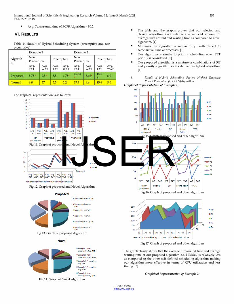
Table 14 (Result of Hybrid Scheduling System (preemptive and non preemptive)
Algorithm
Example 1 Example 2
Non Preemptive
Preemptive Non Preemptive
Preemptive
Avg. TAT
Avg. WAT
Avg. TAT
Avg. WAT
Avg. TAT
Avg. WAT
Avg. TAT
Avg. WAT
Proposed 5.75 * 2.5 * 5.5 1.75* 16.33*
8.66* 15.66
8.0
Normal 6.0 27 5.5 2.2 17.3 9.6 15.6 8.0
The graphical representation is as follows;
Fig 11. Graph of proposed and Novel Algorithm
Fig 12. Graph of proposed and Novel Algorithm
Fig 13. Graph of proposed Algorithm
Fig 14. Graph of Novel Algorithm
The table and the graphs proves that our selected and chosen algorithm gave relatively a reduced amount of average turn around and waiting time as compared to novel algorithm. [1]
Moreover our algorithm is similar to SJF with respect to same arrival time of processes. [1]
Our algorithm is similar to priority scheduling when TET priority is considered. [1]
Our proposed algorithm is a mixture or combinations of SJF and priority algorithm so it’s defined as hybrid algorithm. [1]
i. Result of Hybrid Scheduling System Highest Response
Round Ratio Next (HRRRN)Algorithm: Graphical Representation of Example 1:
Fig 15. Graph of proposed and other algorithm
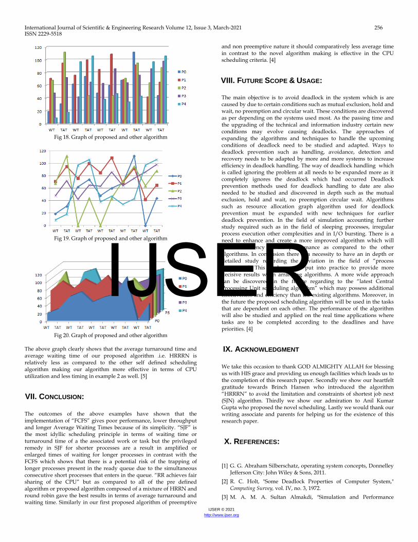
Fig 16. Graph of proposed and other algorithm
Fig 17. Graph of proposed and other algorithm
The graph clearly shows that the average turnaround time and average waiting time of our proposed algorithm .i.e. HRRRN is relatively less as compared to the other self defined scheduling algorithm making our algorithm more effective in terms of CPU utilization and less timing. [5]
The above graph clearly shows that the average turnaround time and average waiting time of our proposed algorithm .i.e. HRRRN is relatively less as compared to the other self defined scheduling algorithm making our algorithm more effective in terms of CPU utilization and less timing in example 2 as well. [5]
VII. CONCLUSION:
The outcomes of the above examples have shown that the implementation of “FCFS” gives poor performance, lower throughput and longer Average Waiting Times because of its simplicity. “SJF” is the most idyllic scheduling principle in terms of waiting time or turnaround time of a the associated work or task but the privileged remedy in SJF for shorter processes are a result in amplified or enlarged times of waiting for longer processes in contrast with the FCFS which shows that there is a potential risk of the trapping of longer processes present in the ready queue due to the simultaneous consecutive short processes that enters in the queue. “RR achieves fair sharing of the CPU” but as compared to all of the pre defined algorithm or proposed algorithm composed of a mixture of HRRN and round robin gave the best results in terms of average turnaround and waiting time. Similarly in our first proposed algorithm of preemptive
and non preemptive nature it should comparatively less average time in contrast to the novel algorithm making is effective in the CPU scheduling criteria. [4]
VIII. FUTURE SCOPE & USAGE:
The main objective is to avoid deadlock in the system which is are caused by due to certain conditions such as mutual exclusion, hold and wait, no preemption and circular wait. These conditions are discovered as per depending on the systems used most. As the passing time and the upgrading of the technical and information industry certain new conditions may evolve causing deadlocks. The approaches of expanding the algorithms and techniques to handle the upcoming conditions of deadlock need to be studied and adapted. Ways to deadlock prevention such as handling, avoidance, detection and recovery needs to be adapted by more and more systems to increase efficiency in deadlock handling. The way of deadlock handling which is called ignoring the problem at all needs to be expanded more as it completely ignores the deadlock which had occurred Deadlock prevention methods used for deadlock handling to date are also needed to be studied and discovered in depth such as the mutual exclusion, hold and wait, no preemption circular wait. Algorithms such as resource allocation graph algorithm used for deadlock prevention must be expanded with new techniques for earlier deadlock prevention. In the field of simulation accounting further study required such as in the field of sleeping processes, irregular process execution other complexities and in I/O bursting. There is a need to enhance and create a more improved algorithm which will ensure efficiency in the performance as compared to the other algorithms. In conclusion there is a necessity to have an in depth or detailed study regarding the deviation in the field of “process generation”. This study can be put into practice to provide more decisive results when arranging algorithms. A more wide approach can be discovered in the future regarding to the “latest Central Processing Unit scheduling algorithm” which may possess additional effectiveness and efficiency than the existing algorithms. Moreover, in the future the proposed scheduling algorithm will be used in the tasks that are dependent on each other. The performance of the algorithm will also be studied and applied on the real time applications where tasks are to be completed according to the deadlines and have priorities. [4]
IX. ACKNOWLEDGMENT
We take this occasion to thank GOD ALMIGHTY ALLAH for blessing us with HIS grace and providing us enough facilities which leads us to the completion of this research paper. Secondly we show our heartfelt gratitude towards Brinch Hansen who introduced the algorithm “HRRRN” to avoid the limitation and constraints of shortest job next (SJN) algorithm. Thirdly we show our admiration to Anil Kumar Gupta who proposed the novel scheduling. Lastly we would thank our writing associate and parents for helping us for the existence of this research paper.
X. REFERENCES:
[1] G. G. Abraham Silberschatz, operating system concepts, Donnelley Jefferson City: John Wiley & Sons, 2011.
[2] R. C. Holt, "Some Deadlock Properties of Computer System," Computing Survey, vol. IV, no. 3, 1972.
[3] M. A. M. A. Sultan Almakdi, "Simulation and Performance
Evaluation of CPU," International Journal of Advanced Research in Computer and Communication Engineering, vol. IV, no. 3, pp. 1-6, 2015.
[4] A. K. Gupta, "Hybrid CPU Scheduling Algorithm," International Journal of Computer Science and Information Technologies, vol. VI, no. 2, pp. 1569-1572, 2015.
[5] A.K.Solanki, "Performance Evaluation of CPU Scheduling by Using Hybrid Approach," International Journal of Engineering Research & Technology, vol. I, no. 4, pp. 1-8, 2012.
[6] International Journal of Modern Engineering Research , vol. II, no. 6,
2012.
[7] S. M. Y. U, "Simulation of CPU Scheduling," vol. II, 2000.
[8] "“CPU Scheduling: A Comparative study," National Conference on Computing for Nation Development, pp. 587-589, 2011.