Deadly Debt Crises: COVID-19in Emerging Markets

Working Paper 2021-03

CRISTINA ARELLANO, YAN BAI AND GABRIELMIHALACHE

April, 2021

Deadly Debt Crises: COVID-19 in Emerging Markets*

Cristina Arellano Yan Bai Gabriel MihalacheFederal Reserve Bank of Minneapolis University of Rochester Stony Brook University

and University of Minnesota and NBER

Current version April 2021. First version May 2020.

Abstract

The coronavirus pandemic has severely impacted emerging markets by generating a large deathtoll, deep recessions, and a wave of sovereign defaults. We study this compound health, economic, anddebt crisis and its mitigation by integrating epidemiological dynamics into a sovereign default model.The epidemic leads to an urgent need for social distancing measures, a large drop in economic activity,and a protracted debt crisis. The presence of default risk restricts fiscal space and presents emergingmarkets with a trade-off between mitigation of the pandemic and fiscal distress. A quantitativeanalysis of our model accounts well for the dynamics of deaths, social distance measures, andsovereign spreads in Latin America. In the model, the welfare cost of the pandemic is higher becauseof financial market frictions: about a third of the cost comes from default risk, compared with a versionof the model with perfect financial markets. We study debt relief programs through counterfactualsand find a compelling case for their implementation, as they deliver large social gains.

Keywords: default risk, sovereign debt, pandemic mitigation, COVID-19, debt relief, official lendingJEL classification: F34, F41, I18

*We thank Mark Aguiar and Manuel Amador for their comment, and Hayagreev Ramesh and Simeng Zeng for excellentresearch assistance. We also thank Stony Brook Research Computing and Cyberinfrastructure and the Institute for AdvancedComputational Science at Stony Brook University for access to the high-performance SeaWulf computing system, which wasmade possible by a $1.4M National Science Foundation grant (#1531492). The views expressed herein are those of the authorsand not necessarily those of the Federal Reserve Bank of Minneapolis or the Federal Reserve System. Contact information:arellano.cristina@gmail.com; yanbai06@gmail.com; mihalache@gmail.com

1 Introduction

The coronavirus pandemic has brought enormous challenges for world economies. To control this highlycontagious and deadly disease, countries have relied on mitigation measures that limit social interactions,while experiencing severe contractions in economic activity. Many governments have also engaged inlarge fiscal transfers to support private consumption in response to the recession. In emerging marketssuch transfer programs have been much smaller because their governments have limited fiscal space,owing to their chronic problems with public debt crises.1 In fact, during the pandemic, many countrieshave defaulted on their sovereign debt (among them Argentina, Ecuador, Ethiopia, and Lebanon), andall emerging markets have experienced increased sovereign spreads. This paper studies the interactionsbetween public debt and the epidemic and shows that susceptibility to debt crises magnifies the economicand health costs of the pandemic.

We develop a framework that integrates standard epidemiological dynamics into a model of sovereigndebt and default. The epidemic triggers a health crisis, with time paths of infected and deceasedindividuals. The government in our model uses public debt but lacks commitment to repay, and thus itmight choose to default, with varying intensity and duration. The economy responds to the epidemicwith social distancing measures that save lives but depress output. The government borrows to supportconsumption during the epidemic, but sovereign default risk limits its ability to do so. The tepidexpansion of government borrowing is nevertheless expensive for the economy because it increases thelikelihood of a lengthy and costly debt crisis. Default risk increases the welfare cost of the epidemic,because by constraining consumption, it increases the cost of social distancing measures needed to fightthe health crisis. We apply our framework to data from Latin America, a region that has experienceda severe COVID-19 outbreak. We fit the model to time series of Google Mobility data and COVID-19daily deaths. We find that the welfare cost of the epidemic is large, about 28% of annual output for thecountry, and also about 7% for its lenders, which hold its outstanding debt upon the outbreak. Thesecosts reflects an elevated death toll of 0.16% of the population, a prolonged debt crisis lasting four years,and significant output losses. We find that sovereign default risk accounts for about a third of thesecosts.

The epidemiological model is the standard susceptible-infected-recovered (SIR) framework. Theepidemic starts when an initial fraction of the population becomes infected. New infections result fromthe interactions of those currently infected with individuals who are susceptible to the disease, as wellas from the degree to which the virus is contagious. The infected individuals transition eventually toeither a recovered state or a deceased state. We follow Alvarez, Argente, and Lippi (2020) and assumethat the death rate depends on the fraction of the population that is currently infected and that socialdistancing measures limit the growth of new infections. The sovereign debt and default frameworkwe adopt follows the one in Arellano, Mateos-Planas, and Rıos-Rull (2019). The sovereign of a smallopen economy borrows internationally and chooses the intensity of default every period, endogenouslydetermining the duration of the default episode. A fraction of the defaulted debt accumulates; it iscapitalized in the stock of outstanding debt, while new credit is endogenously restricted. Partial defaults

1. Gourinchas and Hsieh (2020) were among the first to issue a warning about precarious debt conditions in emergingmarkets and their potential impact on fighting the pandemic. They argue in favor of vigorous international support and a debtmoratorium.

1

in this framework amplify shocks and lead to persistent adverse effects on the economy. We considera centralized problem with a sovereign that values the lives and consumption of the population. Thesovereign decides on borrowing, partial default intensity, and social distancing measures (also referred toas “lockdowns”) to support consumption and manage the infection dynamics with a goal of preventingdeaths. In our framework, default risk responds to the epidemic and shapes its management.

We use a simplified version of our setup, with a finite horizon, to characterize more sharply theinteractions between default risk and epidemic outcomes. Social distancing measures are an investmentin lives and, as such, respond to consumption costs and domestic interest rates, which reflect theshadow cost of borrowing arising from default risk. We show that with perfect financial markets, themarginal cost of social distancing measures tends to be lower, because consumption is determined by theeconomy’s lifetime income. With default, in contrast, lockdowns tend to be inefficiently loose becauseof the higher marginal cost of consumption arising from a lower lifetime income due to default costsand high domestic rates. We show that default risk leads to under-investment in lives and makes theepidemic more deadly.2 We also show that the epidemic leads to an increase in default risk, because ofadditional incentives to borrow.

We evaluate the interaction between financial market frictions and epidemic outcomes in ourquantitative model by comparing our baseline with results in two reference setups: perfect financialmarkets and financial autarky. The epidemic results in sizable loss of life in all economies, but withperfect financial markets, the economy can implement more stringent social distancing measures thatcan reduce the death toll to less than one-third of that in the baseline. Under financial autarky, the deathtoll is about 20% higher than in the baseline. The markedly different health outcomes, together with thedegree to which financial markets can support smooth consumption during the episode across thesemodels, result in sizable differences in the welfare costs of the epidemic.

The fact that financial conditions greatly impact outcomes during the epidemic suggests thatinternational assistance programs can deliver considerable benefits to emerging markets burdened bydefault risk during the COVID-19 pandemic. The International Monetary Fund, the World Bank, theInter-American Development Bank, and other international organizations are sponsoring debt reliefprograms to help countries fight the pandemic. We use our model to conduct two counterfactualexperiments to evaluate such debt relief initiatives. The first program we consider is a default-free,long-term loan by a financial assistance entity. We find that it has large social benefits, increasingthe welfare in the baseline by 7.5% for the country and 4.7% for its lenders. These gains arise from areduction in deaths and a much milder debt crisis, which are due to more efficient mitigation measuresand less reliance on defaultable debt. The second program consists of a voluntary restructuring betweenthe country and its private creditors. We find that upon the outbreak of the epidemic, at our baselineparameterization, the economy and its lenders will voluntarily agree to reduce the debt level by close to10% of output, without affecting the value of debt to lenders. The increase in the market price of theoutstanding debt compensates the loss from holding fewer units. In turn, the economy naturally gainsfrom such a voluntary reduction in its level of debt, by about 11% of output.

Finally, our work makes a methodological contribution. We develop a framework that integrates the

2. Our finding that default risk discourages social distancing measures relates to the debt overhang literature, which hasargued that indebtedness can depress investment, as in Aguiar and Amador (2011).

2

dynamics of defaultable debt with those of epidemiological status in the population. We set up andsolve a Markov problem, in which the government’s choices over debt and social distancing measuresaffect the endogenous evolution of four state variables—namely, the debt and three population groups:susceptible, infected, and recovered. The sovereign lacks commitment and makes current choices, takingas given all future policies. We provide an algorithm that can be adapted to other applications ofepidemiological dynamics in settings with time-varying endogenous aggregate state variables.

The remainder of this section provides a brief review of the relevant literature. The rest of the paperproceeds as follows. Section 2 lays out the structure of our model. Section 3 focuses on a simpler versionof our setup, which enables us to highlight key interactions between deaths, mitigation of the epidemic,and default. Section 4 reports the results for the quantitative analysis of our model, including the dataused to discipline it, counterfactual experiments across alternative financial market arrangements, andthe evaluation of debt relief programs. Section 5 concludes and sets directions for future work.

Literature. Our paper contributes to the fast-growing literature that studies the COVID-19 epidemicand its interactions with economics. Atkeson (2020) was the first to introduce economists to the classicSIR epidemiology model and use it to study the human cost of the COVID-19 epidemic for the UnitedStates. Alvarez, Argente, and Lippi (2020) and Eichenbaum, Rebelo, and Trabandt (2020) study optimalmitigation policies in simple production economies, in which the epidemic dynamics follow a SIR model.Their results highlight the trade-off inherent in lockdowns: they save lives but are costly in terms ofeconomic output. Our epidemiological model follows Alvarez, Argente, and Lippi (2020) setup, butadds consumption smoothing incentives as in Eichenbaum, Rebelo, and Trabandt (2020).

A growing literature considers the role of heterogeneity in the COVID epidemic. Glover, Heathcote,Krueger, and Rıos-Rull (2020) delve into crucial distributional considerations, as the old are moreat risk from the epidemic, yet the young endure most of the economic costs from lockdowns. Theyfind that social distancing and lockdowns are used more extensively by governments with betterability to redistribute. Acemoglu, Chernozhukov, Werning, and Whinston (2020) study lockdowns inenvironments with multiple ages and sectors. They find that smart mitigation strategies that target theold and at-risk population are most helpful. Baqaee, Farhi, Mina, and Stock (2020) and Azzimonti, Fogli,Perri, and Ponder (2020) study how the network structure of sectors and geography can be exploited inthe design of optimal mitigation policies. Guerrieri, Lorenzoni, Straub, and Werning (2020) show thatnegative supply shocks in one sector such as COVID can depress aggregate demand in settings withmultiple sectors and sticky prices. These papers focus on the epidemic’s costs for advanced economiesand have abstracted from the additional challenges in emerging markets. Our paper’s emphasis is onthe additional cost that the epidemic imposes on emerging markets in terms of the resulting debt crises,and to highlight our contribution we have abstracted from additional heterogeneity considerations. Weview our work as complementary to these findings.

A few papers do share our focus on the impact of COVID-19 on emerging markets. Hevia andNeumeyer (2020) highlight the multifaceted nature of the pandemic, a tremendous external shock foremerging markets that includes collapsing export demand, tourism, remittances, and capital flows.Cakmaklı, Demiralp, Kalemli-Ozcan, Yesiltas, and Yildirim (2020) focus on international input-outputlinkages as well as sectoral heterogeneity, by constructing a SIR-macro model calibrated to the Turkish

3

input-output structure, while abstracting from default risk. Espino, Kozlowski, Martin, and Sanchez(2020) study optimal fiscal and monetary policies for emerging markets in a sovereign default modeland model COVID-19 as an unexpected combination of shocks. Similar to our results, they find thatdefault risk increases as a result of the epidemic. Different from us, they do not consider explicitlyepidemiological dynamics and hence their framework is silent on the health crisis.

The dynamic debt and default framework at the core of our work builds on the earlier contributions byEaton and Gersovitz (1981), Aguiar and Gopinath (2006), Arellano (2008), and Chatterjee and Eyigungor(2012). We adopt the more recent approach in Arellano, Mateos-Planas, and Rıos-Rull (2019), whomodel debt crises with partial default and thus an endogenous length of the crisis.This framework givesmeaningful dynamics during default episodes that replicate data, as defaulted debt accumulates overtime and the length of the episode depends on the depth of the recession. Our quantitative evaluation ofdebt relief proposals contributes to the literature on debt buybacks. Like Bulow and Rogoff (1988) andAguiar, Amador, Hopenhayn, and Werning (2019), we find that international lenders would benefit fromdebt buybacks during the COVID-19 epidemic through capital gains. Nonetheless, we emphasize thatthe gains to the country are large and positive because reducing debt overhang can considerably shortenand lessen the debt crisis and save on output costs from default. Furthermore, debt reduction allowsthe country to adopt stricter lockdown policies, which save lives. Our study of voluntary restructuringrelates to the work of Hatchondo, Martinez, and Sosa-Padilla (2014), who evaluate similar proposalsin a setup without epidemic dynamics. They also find scope for Pareto improvements, while focusinginstead on the size of the shock.

2 Model

We consider a small open economy model with a continuum of identical agents and a government thatborrows from the rest of the world, with an option to default on its debt. Output in the economy dependson labor input and productivity. We evaluate the dynamics of this economy after it is unexpectedly hitby an epidemic, COVID-19. The dynamics of infection and deaths follow a standard epidemiological SIRmodel. During the epidemic, a subset of the population endogenously transitions from being susceptibleto being infected. The infected eventually either recover or die. The outcomes of the epidemic can bealtered with social distancing measures, which we often refer to as “lockdowns” as shorthand.

We start by describing preferences, technology, the market for sovereign debt, and the default option.We then discuss the evolution of the disease and social distancing measures, and we formulate thedynamic problem during the epidemic. The outbreak starts when a subset of the population exogenouslybecomes infected.

2.1 Preferences and Technology

We consider preferences over consumption and lives. As in Alvarez, Argente, and Lippi (2020) andFarboodi, Jarosch, and Shimer (2020), the value increases with consumption per capita ct and decreaseswith fatalities φD,t. We assume each fatality imposes a loss of value χ. The lifetime value to the

4

government is

v0 =∞

∑t=0

βt [u(ct)− χφD,t] , (1)

where β is the discount factor. The utility from consumption is concave and equals u(c) = (c1−σ −1)/(1− σ), with σ controlling the intertemporal elasticity of substitution.

Output in the economy Yt is produced using labor, which is impacted by social distancing measures.Agents are endowed with one unit of time, and hence total labor supply equals population Nt. During alockdown of intensity Lt, each agent’s labor input is reduced to (1− Lt).3 The economy’s output equals

Yt = zt [(1− Lt)Nt]α , (2)

where 0 ≤ α ≤ 1 and zt is the economy-wide level of productivity, which depends on an underlyinglevel z and falls with government default.

2.2 Government Debt and Default

The government issues long-term debt internationally and lacks commitment over its repayment. Weconsider a sovereign default model, in which the government can choose to partially default on the debtevery period and thus decides whether to start or end the default episode. We study long-term debt in atractable way by considering random maturity bonds, as do Hatchondo and Martinez (2009). The bondis a perpetuity that specifies a price qt and a quantity `t so that the government receives qt`t units uponthe sale, at time t. In each subsequent period, a fraction δ of the debt matures. Every period, conditionalon not defaulting, each unit of debt calls for a payment of δ + r.4 The government can choose to defaulton a fraction dt of the current payment owed, and it transfers to domestic households all of its proceedsfrom operating in international debt markets. The resource constraint of the economy is given by

Ntct + (δ + r)(1− dt)Bt = Yt + qt`t. (3)

The equilibrium bond price qt is determined by a schedule that depends on the debt level and epidemicdemographics, because as we will see below, the likelihood of future default depends on these states.

In this model with accumulation of long-term defaulted debt, the debt due next period Bt+1 dependsnot only on new issuance `t but also on the outstanding debt Bt and the share of debt on which thegovernment defaults over time. Following Arellano, Mateos-Planas, and Rıos-Rull (2019), we assumethat partial default reduces the current debt service payment to (1− dt)(δ + r)Bt but increases futuredebt obligation by a κ fraction of the defaulted payment. We annuitize these future debt obligationsso that the next period’s debt obligations increase by κdt(δ + r)Bt. Default also depresses productivityto zt = zγ(dt), where the function γ(dt) is decreasing and bounded between 0 and 1. The evolutionof long-term debt is controlled by the new issuance `t, the outstanding debt that has yet to mature,

3. In this baseline model, we have assumed that all individuals, whether they are infected or not, can work equally well. It iseasy to consider an extension in which infected individuals are subjected to a productivity penalty or completely unable towork.

4. We fix this payment level to normalize the risk-free bond price to 1. This normalization does not alter the maturity of thedebt, only the units of our Bt variable.

5

(1− δ)Bt, and any defaulted debt that is carried over:

Bt+1 = `t + [(1− δ) + κ(δ + r)dt] Bt. (4)

International lenders are risk neutral and competitive. They take as given the risk-free rate r, theiropportunity cost. The bond price qt compensates lenders in expectation for their losses due to futuredefaults,

qt =1

1 + r{(δ + r)(1− dt+1) + [1− δ + κ(δ + r)dt+1] qt+1} . (5)

This expression reflects how partial default tomorrow dt+1 reduces the value that lenders get in periodt + 1 but increases the subsequent value to them as the defaulted payments accumulate at rate κ, tobecome due later.

2.3 Epidemic Dynamics

We now describe the outbreak of the epidemic and the subsequent dynamics, which build on the classicSIR structure of Kermack and McKendrick (1927). Following the outbreak of the disease, a subset ofthe population transitions endogenously from being susceptible to being infected and, eventually, tobeing either recovered or deceased. Thus, during the epidemic, the population Nt is partitioned in threeepidemiological groups: susceptible, infected, and recovered. The mass of each group is denoted by µS

t ,µI

t , and µRt , respectively. We assume that the initial population size is 1. The total mass of the deceased is

µDt = 1− Nt. The epidemic starts when an initial mass of the population becomes infected exogenously,

µI0 > 0. The rest are susceptible, except possibly for a measure of agents already recovered µR

0 ≥ 0, sothat µS

0 = 1− µI0 − µR

0 .The spread of the epidemic can be mitigated with lockdowns that limit social interactions, as in

Atkeson (2020) and Alvarez, Argente, and Lippi (2020). These reduce labor input by Lt and socialinteractions by θLt. The parameter θ controls the effectiveness of social distancing measures in preventingthe spread of infection.

A key component of the SIR model concerns how likely it is for susceptible individuals to becomeinfected. We follow the standard approach, according to which their probability of infection depends onthe mass of already infected individuals µI

t and effective social distancing measures θLt. The mass ofnewly infected individuals is denoted by µx

t and we assume that it is determined by

µxt = πx

[(1− θLt)µ

It

] [(1− θLt)µ

St

]. (6)

The presence of 1− θLt twice in the above expression reflects the fact that lockdowns reduce the socialinteractions of both the infected and susceptible. The parameter πx captures the degree to which thedisease is contagious.5 The mass of susceptible individuals in period t + 1 is that of period t net of anynew infections,

µSt+1 = µS

t − µxt . (7)

Infected individuals remain in this state with probability πI . The mass of infected individuals in period

5. In the quantitative analysis in Section 4, we allow πx to be time varying to better capture the lags in timing for mobilityand infections in the data.

6

t + 1 equals a πI share of the infected in period t plus any new infections. The resulting law of motion is

µIt+1 = πIµ

It + µx

t . (8)

With probability 1− πI , each infected individual either recovers or dies. Like Alvarez, Argente, andLippi (2020), we assume that the probability of dying from the disease conditional on being infectedπD(µ

It ) depends on the measure of current infections, resulting in φD,t = πD(µ

It )µ

It fatalities every

period. We assume π′D(µIt ) > 0 to capture the role of health care capacity for the fatality rate; a large

number of infections puts a strain on the health care system, hurting its ability to successfully treat cases.The resolution of infections into recoveries or deaths induces the following laws of motion for these lasttwo groups:

µRt+1 = µR

t +[1− πI − πD(µ

It )]

µIt , (9)

µDt+1 = µD

t + πD(µIt )µ

It . (10)

The epidemic induces a law of motion for the overall population size Nt,

Nt+1 = µSt+1 + µI

t+1 + µRt+1. (11)

As is well known from the epidemiological literature, in such a SIR model, the epidemic eventuallywinds down as the mass of infected individuals asymptotes to zero. Without social distancing measures,the SIR parameters πx, πI , and πD(µ

It ) determine the duration and severity of the outbreak. Social

distancing policies Lt can alter these outcomes. In practice, we adopt an assumption that the epidemicends H periods after it starts because a vaccine becomes available. With the discovery of a vaccine, allsusceptible individuals are vaccinated and become functionally recovered, so no new infections canoccur. This introduces a natural and numerically convenient terminal condition for our analysis, but Hcan be arbitrarily large.

2.4 The Government’s Problem

The government and its international lenders learn about the epidemic in period 0. The outbreakchanges the prospects for the economy, because the epidemic will lead to loss of life and disruptions inproduction. During the epidemic, we set up a centralized problem for the government, which makes allchoices for this economy. It borrows from international financial markets, with an option to default, andchooses lockdown policies Lt to reduce the loss of life from the epidemic.6 We study a Markov problem,which we solve backwards from the vaccine period H.

Consider first the government’s problem for any period before the vaccine arrives t < H. The statevariable for the government consists of the measures of each group µt = (µS

t , µIt , µR

t ) and its debt Bt. Theaccumulated deaths are the residual, µD

t = 1− µSt − µI

t − µRt . The value function for the government

6. We do not study whether households’ own distancing measures would result in activity levels higher or lower than whatis called for by our centralized solution. Farboodi, Jarosch, and Shimer (2020) show that in a similar model but without financialmarket frictions, government-mandated lockdowns improve over private choices, owing to negative externalities in contagion.These findings do not directly translate to our environment because debt crises bring additional negative externalities arisingfrom, e.g., agents who do not internalize that by self-quarantining they are possibly worsening the debt crisis.

7

depends on these states and on time Vt(µt, Bt). The bond price function depends on future states andtime, qt(µt+1, Bt+1), because default decisions will depend on these variables.7 The government takes asgiven future value functions Vt+1(µt+1, Bt+1) and the bond price schedule. It chooses optimal borrowing`t, partial default dt, and lockdowns Lt to maximize its objective, given by

Vt (µt, Bt) = max`t, dt∈[0,1], Lt∈[0,1]

[u(ct)− χφD,t] + βVt+1 (µt+1(µt, Lt), Bt+1) , (12)

subject to the constraint

Ntct + (1− dt)(δ + r)Bt =zγ(dt)[Nt(1− Lt)]α + qt(µt+1(µt, Lt), Bt+1)`t; (13)

the evolution of debt (4); the SIR laws of motion (6)-(9), which map current population measures andlockdown policies to future measures µt+1(µt, Lt); fatalities induced by these dynamics φD,t = πD(µ

It )µ

It ;

and the total population constraint (11). The government internalizes that its choices for debt andlockdown affect the states tomorrow and the bond price.

When choosing Lt, the government trades off the potential benefits from saving lives against the costsof lockdowns in terms of output and consumption. Consumption is lowered by output disruptions fromsocial distancing measures, and this response is amplified by the limited availability of internationalcredit as well as the presence of default risk. If financing opportunities are ample and default risk is low,output disruptions matter for consumption only through a reduction of lifetime income. Consumptionwould then adjust to the lower permanent income, but the period-by-period consumption decline neednot necessarily mirror the contemporaneous declines in output from lockdowns.

The government’s problem results in decision rules for economic variables in periods t = 0, 1, . . . , H−1 for government debt Bt+1 = Bt+1(µt, Bt), default dt = dt(µt, Bt), lockdowns Lt = Lt(µt, Bt), and percapita consumption ct = ct(µt, Bt). The problem also induces policy functions for the evolution ofepidemiological variables that depend on the level of debt as well as the distribution of the populationover types. Debt affects epidemiological dynamics through its impact on lockdowns. Let the equilibriumpolicy functions for the evolution of measures of susceptible, infected, and recovered individuals beµt+1(µt, Bt).

The bond price schedule qt(µt+1(µt, Lt), Bt+1) satisfies

qt(µt+1(µt, Lt), Bt+1) =1

1 + r{(δ + r)(1− dt+1) + [1− δ + κ(δ + r)dt+1] qt+1(µt+2, Bt+2)} ,

where future default, borrowing, and lockdowns are given by equilibrium policy rules from thegovernment problem, and they are taken as given at time t by the government—a Markov environment.The problem from period H onward is similar to the setup described above, except that the vaccine atperiod H moves all the susceptible agents to the recovered state and resolves all infections. Appendix Bprovides a definition of the equilibrium.

7. The time dependency of these functions, captured by the t subscript, reflects the time horizon to the vaccine. They wouldbe time invariant without a terminal condition. The results of the baseline quantitative analysis are not sensitive to the timingof vaccination, as long as it is far enough into the future, as illustrated in Section 4.6.

8

3 Interactions between the Health and Debt Crises

In this section we simplify our model to characterize analytically the interactions between the health anddebt crises. We establish that the epidemic increases default risk, which in turn worsens the epidemic.Social distancing and lockdowns work as investments in lives, and default risk limits the economy’sability to tap future resources, resulting in inefficiently low investment—an inefficient lockdown.8

The simplified model has only two periods. The economy starts without any debt B0 = 0 and withinitial measures of susceptible µS

0 , infected µI0, and recovered µR

0 individuals. The value of the governmentis over consumption and life, [u(c0)− χφD,0] + β[u(c1)− χφD,1]. In period 0, the government chooseslockdowns L0, borrowing B1, and consumption c0. In period 1, it chooses default d1 and consumption c1.

The lockdown L0 reduces new infections in period 0, thereby reducing deaths in period 1. Specifically,we can write period 1’s deaths as φD,1(L0) = πD(µ

I1(L0))µI

1(L0), with the infected mass coming fromboth the unresolved initial infections and the newly infected, µI

1(L0) = πIµI0 + πx(1− θL0)2µI

0µS0 . We

assume φD,1(L0) is decreasing and convex in lockdowns L0, ∂φD,1/∂L0 ≤ 0 and ∂φ2D,1/∂L2

0 ≤ 0. Sincethe government cannot alter deaths in period 0, φD,0, or population in period 1, N1, as both are pinneddown by the initial level of infection and epidemiology parameters, we assume for simplicity zero initialdeaths, φD,0 = 0. For a cleaner exposition, we also restrict attention to θ = 1 and linear production,α = 1. Appendix D lays out the details of this stripped-down version of our model and the assumptionsthat guarantee an interior solution for partial default d1 and lockdown L0. In particular, we require thatthe output in default zγ(d) is differentiable, decreasing, and concave in d.

We construct the solution to the government’s problem working backwards. In period 1, thegovernment cannot borrow and only chooses partial default to weigh its marginal benefit and cost,−zγ′(d1) = B1, where −zγ′(d1) reflects the marginal cost of a higher default intensity in terms of lostproduction and B1 is the marginal benefit of lowering repayment. Let the optimal default decision bed1(B1) = (γ′)−1(−B1/z), with (γ′)−1 the inverse of the derivative of γ. Under the assumption thatγ(d1) is concave, partial default d1 increases with B1. The bond price schedule in period 0 reflects these

default incentives, satisfying q0(B1) =1

1 + r(1− d1(B1)).

In period 0, the government chooses borrowing B1 and lockdowns L0. We derive a standardoptimality condition for the borrowing choice as

u′(c0) = β(1 + rd(B1))u′(c1),

where 1 + rd(B1) is the domestic interest rate. It depends on the risk-free rate and on the elasticity ofthe bond price schedule with respect to borrowing 1 + rd(B1) = (1 + r)/(1− η(B1)), where η(B1) =

−∂ ln(q0)/∂ ln(B1) ≥ 0. The domestic interest rate reflects the shadow cost of borrowing and withdefault risk, it is higher than the risk-free rate, rd(B1) ≥ r. The consumption in period 0 is then a fractionof lifetime income that decreases with the domestic interest rate, so that

c0 =1

1 + 11+r [β(1 + rd(B1))]1/σ

(z(1− L0) +

11 + r

zγ(d1)

), (14)

8. This mechanism is linked to the literature emphasizing the impact of limited enforcement on under-investment, exampleof which include Thomas and Worrall (1994) and Aguiar and Amador (2011).

9

where period 0 income z(1− L0) depends on the lockdown policy and period-1 income is shaped by thedefault cost zγ(d1) and is discounted at the risk free rate 1 + r.

The optimal lockdown L0 equates the marginal cost of reducing current consumption c0 to themarginal benefit of saving lives in period 1. Future default risk d1 reduces lifetime income and tends toreduce current consumption c0, which in turn increases the cost of lockdowns. We capture these forceswith the following optimality condition:

zu′(c0) = βχ

(−∂φD,1(L0)

∂L0

). (15)

The left-hand side of (15) is the marginal cost of lockdowns in terms of reducing current consumption.For one extra unit of lockdown, output drops by z units, which are worth zu′(c0). The right-hand siderepresents the marginal value of lockdowns in terms of saving lives. One extra unit of lockdown reducesdeaths by (−∂φD,1/∂L0), which is worth χ(−∂φD,1/∂L0) ≥ 0, given that χ is the value of one life.

With the following propositions, we establish that the health and debt crises reinforce each other. Wefirst show that the pandemic leads to a higher default risk in period 1.

Proposition 1 (The epidemic generate default risk). The default intensity d1 increases following an epidemicoutbreak in period 0.

See Appendix D for the proof. The epidemic generates default risk because a desire to smoothconsumption induces higher borrowing and thus a higher default risk in the future. The increaseddefault risk worsens financial conditions in period 0. In our general model, there are two additionalmechanisms that lead to more default. First, following an unexpected epidemic outbreak in the firstperiod, lockdowns lower the marginal cost of defaulting, and partial default increases. Second, lendersinternalize poor future prospect which tighten the bond price schedule for long-term debt. Highborrowing rates further increase higher default incentives.

Next, we illustrate our second point: future default risk reduces lockdown incentives and worsensthe epidemic. To show this, we introduce a reference model with perfect financial markets, in which thegovernment commits to fully repaying its debt; that is, d1 = 0. We establish that the lockdown intensityin our baseline model is lower than the efficient level from the setup with perfect financial markets. Withlimited enforcement, the economy tends to “under-invest” in life-saving measures and ends with toomany deaths.

With full commitment, the government chooses consumption and lockdown to maximize its value,subject to the evolution of the epidemic and a lifetime budget constraint. The optimal lockdown in thiscommitment setup also satisfies equation (15). Perfect financial markets, however, allow the country tosmooth consumption across time and support a higher level of consumption in period 0, ce

0. Specifically,consumption in period 0, ce

0, satisfies

ce0 =

11 + 1

1+r [β(1 + r)]1/σ

(z(1− Le

0) +1

1 + rz)

, (16)

where Le0 is the lockdown in this case. For a given lockdown L0, consumption in period 0 is higher with

perfect financial markets for two reasons. First, permanent income under perfect financial markets is

10

higher than in the baseline model because of the absence of default costs. Second, the share of permanentincome allocated for c0 is also higher because the domestic interest rate is given by the risk-free rater, which is lower than the one with default risk, rd(B1). Increased consumption reduces the cost oflockdowns and generates a more intense lockdown in the perfect financial markets case.

Proposition 2 (Default risk worsens the epidemic). Deaths are higher with default risk than in an economywith perfect financial markets.

See Appendix D for the proof. With default risk, the consumption cost of social distancing is higher,which results in lockdowns of lower intensity. Less mitigation elevates infections and results in moredeaths.

4 Quantitative Analysis

We now turn to the quantitative analysis of the general model. Our goal is a quantitative evaluation ofour mechanisms and policy counterfactuals. We first discuss the choice of parameters, including thosecontrolling the SIR dynamics and the cost of default, and our moment-matching exercise with data fromLatin America. We then describe the time paths of the economy and assess quantitatively the extent ofthe health, economic, and debt crises. To highlight financial markets’ role for epidemic dynamics, wecompare these time paths with those of two reference models, one with perfect financial markets andanother with financial autarky. Finally, we conduct counterfactual debt relief experiments and show thatthese programs can deliver large social gains.

4.1 Parameterization and Data

We consider a weekly model to capture the fast dynamics of infection. We fix some of the parametersto values from the literature and estimate others with a moment-matching exercise to data from LatinAmerica.

Epidemiological parameters. The SIR parameters are set based on findings in epidemiological research.According to Wang et al. (2020), the duration of illness is on average 18 days.9 For our weekly model thisimplies a value for πI , the parameter determining the rate at which infected individuals either recoveror die from the disease, of (1− 1/18)7 = 0.67.

The parameter πx relates to the widely used “reproduction number” R0, which measures theexpected number of additional infections caused by one infected person over the entire course of hisor her illness, with πx = (1− πI)R0. As shown by Atkeson, Kopecky, and Zha (2020), the data oninfections and deaths from COVID-19 are useful for recovering the underlying effective reproductionnumber for the epidemic, as non-pharmaceutical interventions, such as masking and testing, influencethe degree to which the infection is transmitted and thus the value of this number. To that end, weassume that R0,t is time varying because of health policies and behavioral responses. We impose asimple functional form controlled by the initial and final reproduction numbers {R0,ini,R0,end} and a

9. This is also the value used by Atkeson (2020) and Eichenbaum, Rebelo, and Trabandt (2020).

11

decay rate ρ such that R0,t = R0,ini ρt +R0,end(1− ρt). We set the R0,ini to 2.6, based on early estimatesof the reproduction number, including those from the Diamond Princess cruise ship, and estimate theother two parameters to Latin American data, as explained below.10

Following Alvarez, Argente, and Lippi (2020), we assume the case fatality rate πD(µIt ) depends

on the number of infected individuals to capture congestion effects in the healthcare system, sothat πD(µ

It ) = π0

D + π1DµI

t . The parameters π0D and π1

D control the mortality of the infected. Weassume that, in the absence of health care capacity constraints, the fatality rate is 0.5%, which iswithin the range of parameters used in recent papers studying COVID-19. Using this estimate, we setπ0

D = (1− πI)× 0.005 = 0.0016, and we estimate π1D to fit the data. The lockdown effectiveness is set to

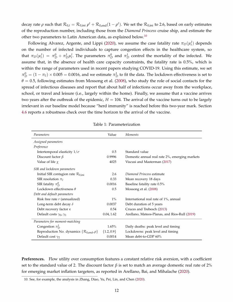
θ = 0.5, following estimates from Mossong et al. (2008), who study the role of social contacts for thespread of infectious diseases and report that about half of infections occur away from the workplace,school, or travel and leisure (i.e., largely within the home). Finally, we assume that a vaccine arrivestwo years after the outbreak of the epidemic, H = 104. The arrival of the vaccine turns out to be largelyirrelevant in our baseline model because “herd immunity” is reached before this two-year mark. Section4.6 reports a robustness check over the time horizon to the arrival of the vaccine.

Table 1: Parameterization

Parameters Value Moments

Assigned parametersPreference

Intertemporal elasticity 1/σ 0.5 Standard valueDiscount factor β 0.9996 Domestic annual real rate 2%, emerging marketsValue of life χ 4025 Viscusi and Masterman (2017)

SIR and lockdown parametersInitial SIR contagion rate R0,ini 2.6 Diamond Princess estimateSIR resolution πI 0.33 Mean recovery 18 daysSIR fatality π0

D 0.0016 Baseline fatality rate 0.5%Lockdown effectiveness θ 0.5 Mossong et al. (2008)

Debt and default parametersRisk free rate r (annualized) 1% International real rate of 1%, annualLong-term debt decay δ 0.0037 Debt duration of 5 yearsDebt recovery factor κ 0.54 Cruces and Trebesch (2013)Default costs γ0, γ1 0.04, 1.62 Arellano, Mateos-Planas, and Rıos-Rull (2019)

Parameters for moment-matchingCongestion π1

D 1.65% Daily deaths: peak level and timingReproduction No. dynamics {R0,end, ρ} {1.2, 0.9} Lockdowns: peak level and timingDefault cost γ2 0.0014 Mean debt-to-GDP 60%

Preferences. Flow utility over consumption features a constant relative risk aversion, with a coefficientset to the standard value of 2. The discount factor β is set to match an average domestic real rate of 2%for emerging market inflation targeters, as reported in Arellano, Bai, and Mihalache (2020).

10. See, for example, the analysis in Zhang, Diao, Yu, Pei, Lin, and Chen (2020).

12

An important parameter for our model is the cost of losing a life, χ. This parameter relates to thevalue of statistical life (VSL), which measures the marginal willingness to take on mortality risk. Viscusiand Masterman (2017) report estimates of the VSL across countries in 2015, and in our calculation weuse their estimate of 1.695 million for Brazil.11 Using an annual interest rate of 2% and a residual life of40 years, we can express the VSL in terms of a weekly flow of $1,200, which implies a willingness to payof $1.2 (or 0.85% weekly consumption) for 0.1% of reduction in mortality risk.12 We use this calculationto set χ as the solution to the following equation:

1− β10×52

1− βu(1)− 0.001χ =

1− β10×52

1− βu(1− 0.0085),

where we assume that the representative COVID-19 fatality has 10 years of residual life. The impliedvalue for χ is 4,025, given our parameter values for β and the coefficient of relative risk aversion.

Debt and default. We set the annual international risk-free rate to 1%, which is the average real ratefor U.S. Treasury bills since 1985. We pick δ to induce an average Macaulay debt duration of five years,in line with estimates for emerging markets. As in Arellano, Mateos-Planas, and Rıos-Rull (2019), weassume that the default cost is a concave function of the default intensity, γ(d) = [1− γ0dγ1 ](1− γ21d>0),where the indicator 1d>0 is 1 if d is positive so that a share γ2 of productivity is lost if the countrydefaults at all, with any intensity. We adopt estimates for γ0 and γ1 from Arellano, Mateos-Planas, andRıos-Rull (2019) and estimate the fixed cost parameter γ2. The debt recovery κ is set to 0.54, consistentwith the evidence in Cruces and Trebesch (2013), once preemptive restructurings are excluded. We setz = 1, a normalization of pre-pandemic steady state output to 1. The top panel in Table 1 collects allassigned parameter values.

Data. We compile data from Latin America for eleven countries: Argentina, Brazil, Chile, Colombia,Ecuador, El Salvador, the Dominican Republic, Mexico, Peru, Paraguay, and Uruguay. We collect timeseries during the year 2020 for deaths from the COVID-19 epidemic, Google Mobility data, governmentdebt, and sovereign spreads.

The measure for deaths is average daily deaths per 10,000 people, monthly for the year 2020. Thisinformation is taken from the worldometers.info (2021) website. The Google Mobility measure we useis the weekly decline in workplace traffic13 relative to January 2020, provided by Google LLC (2021).We compare our model with the average data series from these countries at a monthly frequency. Inconstructing these time series, we first time-aggregate weekly observations into monthly series and thenaverage these monthly series across countries, weighting each country’s value by its population in 2019.

11. In practice, the VSL estimates of Viscusi and Masterman (2017) do not vary much among countries. In terms of annualconsumption per capita, they find that the VSL is 184 for Argentina, 229 for Brazil, 224 for Mexico, and 207 for the U.S.

12. To calculate the weekly flow, we solve for x in

1.695× 106 =1− 0.999640×52

1− 0.9996x,

which implies x = 1, 200. The consumption data is in terms of 2015 U.S. dollar, from the World Bank.13. Workplace traffic data imply an upper bound on the reduction in activity, as some work could be done from home.

Nevertheless, Dingel and Neiman (2020) and Saltiel (2020) find that in developing countries only a minority of jobs can beperformed at home: at most 25%, but as low as 10% for Colombia and Ecuador.

13

The data for government debt are taken from local primary sources such as each country’s centralbank, statistics office, or finance ministries. We compile quarterly data for 2019 and 2020 and report debtrelative to gross domestic product. To set the initial debt level, we use the data in the fourth quarter of2019 averaged across countries, weighting by population in 2019. The data for sovereign spreads arethe EMBI+ series for all the countries for which they re available at a monthly frequency for the year2020. The data are from Global Financial Data (2021). We average across countries, again weighting bypopulation, and report the resulting time series relative to its value in January 2020.

The first column of Table 2 reports select moments for the data. The COVID-19 epidemic has hit LatinAmerican countries quite hard, as seen in the data on daily deaths and lockdowns. Daily deaths peakedat 0.047 per 10,000 people during July 2020 and were 0.03 on average for the year. Google Mobility dataimply that workplace hours were reduced by 48% at the trough during April 2020 and on average by21%. The table also reports elevated sovereign spreads, peaking at 5.5% above their January level. Thetable finally shows that government debt to output across these countries was on average 60% at theonset of the epidemic.

4.2 Model Fit

We now describe our moment-matching exercise and the fit of the model. We estimate four parametersof our structural model: two controlling the dynamics of the epidemiological reproduction number, Rend

and ρ; the fatality parameter π1D; and the fixed cost of default γ2. We do so by targeting five moments of

the data: the peak and timing of the daily deaths, the peak and timing of lockdowns, and the initialgovernment debt to output ratio.

We interpret the data as being in steady state during January of 2020. In a pre-pandemic steadystate, the model features an endogenous debt to output ratio, which we fit by choosing the fixed costof default. We start the epidemic in the model in the first week of April 2020 by introducing a smallfraction of infected individuals into the population, µI

0 = 0.5%, and 3% of these already recovered orimmune to the disease, µR

0 = 3%. We then compute and simulate the model, to calculate the relevanttime paths. We compare the model with our daily deaths data by multiplying the model weekly deathsper population, πD(µ

It )µ

It , by 10, 000/7 to scale it to the relevant daily number and average across four

weeks. We compare lockdowns in our model directly with the Google Mobility measure.Appendix E describes our computational algorithm. To summarize it, we first compute the model

without an epidemic. This serves as an initial condition and provides the basis of the economy afterthe epidemic. We then compute our benchmark model backwards, starting from the terminal periodH when the vaccine arrives. As shown in the Appendix, the period H problem is very similar to thepre-epidemic problem, as no new infections occur. The solution consists of time-dependent bond prices,policy, and value functions. We then simulate forwards given our initial conditions, to construct theeconomy’s paths during the epidemic.

Table 2 presents the model fit. In our model, daily death peak at 0.047 in July 2020, which matches thedata. The model also generates a sizable lockdown of 41% during April 2020, close to the correspondingdata value. Debt to output also matches well the value observed in the data. An important aspect of ourparameterization, which enables this fit, is the time-varying reproduction number R0,t, especially withrespect to the asynchronicity between the peaks of daily deaths and lockdowns. The model rationalizes

14

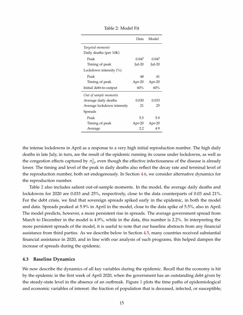
Table 2: Model Fit

Data Model

Targeted momentsDaily deaths (per 10K)

Peak 0.047 0.047Timing of peak Jul-20 Jul-20

Lockdown intensity (%)

Peak 48 41Timing of peak Apr-20 Apr-20

Initial debt-to-output 60% 60%

Out of sample momentsAverage daily deaths 0.030 0.033Average lockdown intensity 21 25

Spreads

Peak 5.5 5.9Timing of peak Apr-20 Apr-20Average 2.2 4.9

the intense lockdowns in April as a response to a very high initial reproduction number. The high dailydeaths in late July, in turn, are the result of the epidemic running its course under lockdowns, as well asthe congestion effects captured by π1

D, even though the effective infectiousness of the disease is alreadylower. The timing and level of the peak in daily deaths also reflect the decay rate and terminal level ofthe reproduction number, both set endogenously. In Section 4.6, we consider alternative dynamics forthe reproduction number.

Table 2 also includes salient out-of-sample moments. In the model, the average daily deaths andlockdowns for 2020 are 0.033 and 25%, respectively, close to the data counterparts of 0.03 and 21%.For the debt crisis, we find that sovereign spreads spiked early in the epidemic, in both the modeland data. Spreads peaked at 5.9% in April in the model, close to the data spike of 5.5%, also in April.The model predicts, however, a more persistent rise in spreads. The average government spread fromMarch to December in the model is 4.9%, while in the data, this number is 2.2%. In interpreting themore persistent spreads of the model, it is useful to note that our baseline abstracts from any financialassistance from third parties. As we describe below in Section 4.5, many countries received substantialfinancial assistance in 2020, and in line with our analysis of such programs, this helped dampen theincrease of spreads during the epidemic.

4.3 Baseline Dynamics

We now describe the dynamics of all key variables during the epidemic. Recall that the economy is hitby the epidemic in the first week of April 2020, when the government has an outstanding debt given bythe steady-state level in the absence of an outbreak. Figure 1 plots the time paths of epidemiologicaland economic variables of interest: the fraction of population that is deceased, infected, or susceptible;

15

the intensity of social distancing measures; government debt and spreads; consumption; and output.The paths run through January 2023, and the vertical lines in the plots represent the date at which thevaccine arrives.

Panel (a) of Figure 1 plots the evolution of the deceased µDt . Our model predicts that the eventual

death toll from the epidemic is 0.16% of the population, which corresponds to 840,000 people for theLatin American countries in our data, with a total population of 525 million in 2019. Panel (b) plotslockdowns and shows that they start promptly upon the outbreak, remain at a 40% level for about twomonths, gradually wind down, and last about a year. These social distancing measures reduce the deathtoll of the epidemic. At our parameter estimates, if we were to impose no social distancing measuresduring the epidemic, the SIR laws of motion would predict a death toll of 1.23% of the population, or6.5 million people in the Latin American countries of our sample.

Figure 1’s panels (c) and (d) plot the evolution of infected and susceptible measures during theepisode. The infected portion of the population reaches its peak of 1.2% in July 2020. The fraction ofsusceptible individuals falls smoothly as the epidemic progresses, until about 75% of the populationis still vulnerable to infection. After two years the vaccine arrives and all the remaining susceptibleindividuals become immune, but the vaccine comes late, as the brunt of infections have passed and thecountry is close to “herd immunity.”

Panels (e) and (f) show the paths of sovereign spreads and government debt scaled by outputbefore the epidemic. Spreads jump on impact by about 6% and decrease smoothly thereafter. Theyincrease because the epidemic is unexpected and increases default risk. Government debt grows becauseadditional borrowing is useful to support consumption and also because the government partiallydefaults on the debt, with defaulted payments accumulating. Debt to output increases until January2021, when it reaches a peak of about 70% of initial output. The 10% increase in debt to output resemblesthe experiences of Latin American countries, which experience an increase in debt to output of 11%on average.14 Afterwards debt falls, but quite slowly, as the economy converges to steady state afterJanuary 2023, about a year after the epidemic resolves. The persistently high level of debt during theepidemic leads to a prolonged period of elevated sovereign spreads and partial default.

Finally, panels (g) and (h) in Figure 1 show the paths for output and consumption. Output fallssignificantly at the outset of the epidemic because of the tight lockdowns. During 2020, output falls inthe model by about 18%. Consumption falls too, by about 6.5%. The consumption decline is smallerthan that of output because government borrowing and default support consumption. During 2021 and2022, levels of consumption and output continue to be lower than they are in the steady state; they areabout 5% below their pre-epidemic levels. Resources are fewer because of the default costs associatedwith the protracted debt crisis. The economy approaches the steady state by early 2023.

These time paths suggest that the epidemic creates a combined health, debt, and economic crisiswith scarring effect on output, consumption, and sovereign spreads that are more persistent than thehealth crisis itself.

14. Although we do not have data for all countries in our sample, we have used the available data for Brazil, Ecuador, Mexico,Paraguay, and Peru, in computing this average.

16

Figure 1: Dynamics in Baseline Model

Jan 2020 Jan 2021 Jan 2022 Jan 20230

0.02

0.04

0.06

0.08

0.1

0.12

0.14

0.16

(a) Deceased

Jan 2020 Jan 2021 Jan 2022 Jan 20230

0.05

0.1

0.15

0.2

0.25

0.3

0.35

0.4

0.45

(b) Lockdowns

Jan 2020 Jan 2021 Jan 2022 Jan 20230

0.2

0.4

0.6

0.8

1

1.2

1.4

(c) Infected

Jan 2020 Jan 2021 Jan 2022 Jan 202370

75

80

85

90

95

100

Vaccine

(d) Susceptible

Jan 2020 Jan 2021 Jan 2022 Jan 202360

62

64

66

68

70

72

(e) Debt

Jan 2020 Jan 2021 Jan 2022 Jan 20230

1

2

3

4

5

6

(f) Spread

Jan 2020 Jan 2021 Jan 2022 Jan 20230.65

0.7

0.75

0.8

0.85

0.9

0.95

1

(g) Output

Jan 2020 Jan 2021 Jan 2022 Jan 20230.82

0.84

0.86

0.88

0.9

0.92

0.94

0.96

0.98

1

(h) Consumption

Notes: Deceased, Infected, and Susceptible are expressed in percentage of population. Debt is relative to pre-pandemic output. Spread is inpercentage, relative to January 2020 value. Output and consumption are relative to pre-pandemic output.

17

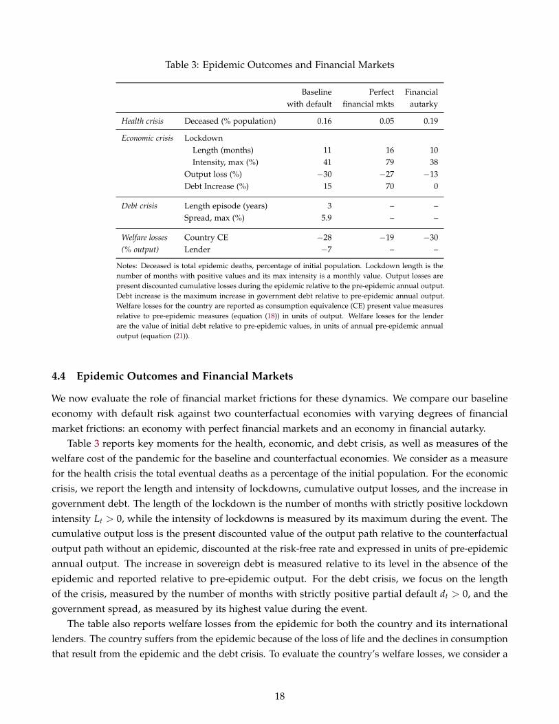
Table 3: Epidemic Outcomes and Financial Markets

Baseline Perfect Financialwith default financial mkts autarky

Health crisis Deceased (% population) 0.16 0.05 0.19

Economic crisis LockdownLength (months) 11 16 10Intensity, max (%) 41 79 38

Output loss (%) −30 −27 −13Debt Increase (%) 15 70 0

Debt crisis Length episode (years) 3 – –Spread, max (%) 5.9 – –

Welfare losses Country CE −28 −19 −30(% output) Lender −7 – –

Notes: Deceased is total epidemic deaths, percentage of initial population. Lockdown length is thenumber of months with positive values and its max intensity is a monthly value. Output losses arepresent discounted cumulative losses during the epidemic relative to the pre-epidemic annual output.Debt increase is the maximum increase in government debt relative to pre-epidemic annual output.Welfare losses for the country are reported as consumption equivalence (CE) present value measuresrelative to pre-epidemic measures (equation (18)) in units of output. Welfare losses for the lenderare the value of initial debt relative to pre-epidemic values, in units of annual pre-epidemic annualoutput (equation (21)).

4.4 Epidemic Outcomes and Financial Markets

We now evaluate the role of financial market frictions for these dynamics. We compare our baselineeconomy with default risk against two counterfactual economies with varying degrees of financialmarket frictions: an economy with perfect financial markets and an economy in financial autarky.

Table 3 reports key moments for the health, economic, and debt crisis, as well as measures of thewelfare cost of the pandemic for the baseline and counterfactual economies. We consider as a measurefor the health crisis the total eventual deaths as a percentage of the initial population. For the economiccrisis, we report the length and intensity of lockdowns, cumulative output losses, and the increase ingovernment debt. The length of the lockdown is the number of months with strictly positive lockdownintensity Lt > 0, while the intensity of lockdowns is measured by its maximum during the event. Thecumulative output loss is the present discounted value of the output path relative to the counterfactualoutput path without an epidemic, discounted at the risk-free rate and expressed in units of pre-epidemicannual output. The increase in sovereign debt is measured relative to its level in the absence of theepidemic and reported relative to pre-epidemic output. For the debt crisis, we focus on the lengthof the crisis, measured by the number of months with strictly positive partial default dt > 0, and thegovernment spread, as measured by its highest value during the event.

The table also reports welfare losses from the epidemic for both the country and its internationallenders. The country suffers from the epidemic because of the loss of life and the declines in consumptionthat result from the epidemic and the debt crisis. To evaluate the country’s welfare losses, we consider a

18

consumption equivalence measure ceq(µ0, B0) at the outbreak of the epidemic, implicitly defined by

11− β

u(ceq(µ0, B0)) = V0(µ0, B0), (17)

where V0(µ0, B0) is the value function at time 0, at the outbreak of the epidemic, that is, the first week ofApril 2020. The value function V0 reflects both the stream of consumption and the stream of deaths; ourconsumption equivalence measure summarizes these two streams into one value, which is the constantconsumption flow that equals this value in the absence of any mortality risk. Using the country’sdiscount β, we express the welfare loss as the present value of the consumption equivalence losses:

CE present value =ceq(µ0, B0)− cpre,eq(B0)

1− β, (18)

where cpre,eq(B0) is the pre-epidemic consumption equivalence when debt is B0.Lenders also suffer losses because the epidemic triggers a debt crisis that they did not anticipate, a

drop in the value of the bonds they hold, effectively a capital loss. We report these losses as the changein the value of initial debt B0 for the bond holders, which depends on the market price of this debt uponthe outset of the epidemic, q(µ0, B0):

Lenders’ value(B0) = q(µ0, B0)B0. (19)

This bond price depends on the structure of our long-term debt contracts, as well as current and futuredefaults. Recall that every unit of outstanding debt decays at rate δ, calls for a payment of (δ + r) everyperiod without default, and accumulates at rate κ per defaulted unit when dt > 0. In addition, note thatthe bond price function at time 0, q0(µ1(µ0, L0), B1), as specified in equation (5), compensates for theexpected default losses from period 1 onward. This implies that the effective price of the outstandingdebt upon the onset of the epidemic, before any decisions, is equal to

q(µ0, B0) = (1− d0(µ0, B0))(δ + r) + [1− δ + κ(δ + r)d0(µ0, B0)]q0(µ1, B1), (20)

where the states {µ1, B1} are given by the government’s decision rules, given initial conditions {µ0, B0}.We report welfare losses for lenders as the change in their value relative to the pre-epidemic value:

Lenders’ loss = q(µ0, B0)B0 − qpre(B0)B0, (21)

where qpre(B0) is the bond price before the epidemic. We report losses in units of pre-epidemic annualoutput.

Baseline economy. Consider again the outcomes in the baseline model with default risk, capturedby the first column of Table 3. These statistics summarize the time paths presented in Figure 1. Theepidemic results in a final death toll of 0.16% of the population, and lockdowns are in effect for 11months, with a peak intensity of 41%. The output losses from the epidemic equal 30% in presentvalue; about half of the losses are due to lockdowns, and the other half are due to default costs. The

19

government debt to output ratio increases by 10 percentage points to support consumption. The debtcrisis lasts about four years, with elevated spreads and partial default. Table 3 reports that the welfarelosses from the epidemic are significant: for the country 28% in terms of pre-epidemic output, whichcorresponds to a 0.6% drop in consumption equivalence every period. Lenders are also worse off byabout 7%, owing to unexpected capital losses. The burden of the epidemic falls largely on the country.

We now compare the results of our baseline economy with those of our two reference economies,which have varying financial market conditions. For these comparisons, we keep all the structuralparameters fixed across economies. Further details on these reference models are in Appendix C.

Perfect financial markets. In the reference model with perfect financial markets, the economy canfreely borrow at the risk-free rate to support consumption, and social distancing measures affectconsumption only through their effect on the present value of output. The epidemic outcomes for aneconomy with perfect financial markets are presented in the second column of Table 3.

With access to perfect financial markets, the economy fares substantially better. Total deaths aresharply cut to less than a third, about 0.05% of the population. The time path of daily deaths exhibitsa much lower peak at 0.01, compared with the baseline’s peak of 0.047. Such a reduction in fatalitiesis due to the longer and more intense lockdowns. Social distancing measures in this economy lastfor 16 months and are at a higher intensity, with a maximum level of 79%.15 The present value ofoutput losses in this case is somewhat smaller than in the baseline; in this economy, it is equal to 27%.The main difference with the baseline is that the output losses in this model arise strictly because oflockdowns and not because of default costs, which means the output costs in this economy are directlylinked to investment in saving lives. Government debt is used aggressively to support consumption andincreases by 70%.16 With perfect financial markets, the economy does not experience a debt crisis, withits associated partial default and elevated government spreads. The welfare costs from the epidemiccontinue to be quite significant for the country while it does not affect lenders. During the epidemic,welfare is 19% lower than it was in the pre-epidemic economy. Comparing this welfare cost with the28% one in the baseline, suggests that default risk accounts for over a third of the cost of the epidemic inthe baseline.

Financial autarky. We also consider outcomes in a counterfactual economy that experiences theepidemic without access to borrowing and remains in financial autarky throughout. Without marketaccess, lockdowns affect consumption one-for-one and period-by-period and the epidemic results inworse outcomes. Without the possibility of external borrowing, the cost of social distancing is larger,leading to a choice of shorter and more limited lockdowns. The less stringent mitigation policies resultin a higher death toll. The eventual death toll is 0.19% of the population, or about 20% more deaths thanin the baseline. The output costs are more muted than in the baseline for two reasons. First, lockdownsare shorter with financial autarky, and second, the government does not experience any default costs.Finally, we find that the welfare costs from the epidemic are slightly higher under financial autarky

15. The decrease in fatalities with perfect financial markets goes a long way towards the minimum feasible fatalities from theepidemic, as discussed in Hethcote (2000) and the pedagogical exposition in Moll (2020).

16. With perfect financial markets, the economy has an incentive to increase borrowing even without the epidemic. To isolatethe effect of the epidemic, we report the increase in debt relative to this preexisting trend.

20

because of the higher death toll and an inability to smooth consumption.

Figure 2: Epidemic Dynamics and Financial Markets

Jan 2020 Jan 2021 Jan 2022 Jan 20230

0.05

0.1

0.15

0.2

Autarky

Perfect Fin. Mrkts

Baseline

(a) Deceased

Jan 2020 Jan 2021 Jan 2022 Jan 20230

0.1

0.2

0.3

0.4

0.5

0.6

0.7

0.8

Baseline

Perfect Fin. Mrkts

Autarky

(b) Lockdown

Jan 2020 Jan 2021 Jan 2022 Jan 20230.7

0.75

0.8

0.85

0.9

0.95

1

1.05

Perfect Fin. Mrkts

Baseline

Autarky

(c) Consumption

Dynamics. Figure 2 compares the time paths of the deceased population, lockdowns, and consumptionin our baseline model with those of two reference economies. The paths are plotted relative to thosethat would arise in the absence of the epidemic. The accumulation of deaths in panel (a) illustrates thataccess to better financial markets can be a powerful tool to dampen the costs of the health crisis andthat sovereign default risk is literally deadly for an economy that faces an epidemic. These radicallydistinct outcomes for the evolution of deaths reflect the different lockdown policies implemented underthese financial market conditions; such policies are presented in panel (b). The economy with perfectfinancial markets can support more stringent social distancing because it can use financial resources tosupport consumption. At the other extreme, financial autarky forces the government to pick less strictlockdowns, as the lost output translates one-to-one into lower current consumption.

The consumption paths for the three financial settings are compared in panel (c) of Figure 2. Withperfect financial markets, consumption falls only to the extent called for by the decline in permanentincome from the lockdowns. Consumption has a downward trend because the economy is moreimpatient than international lenders, as the parameters satisfy β(1 + r) < 1. Under financial autarky,consumption experiences the sharpest declines during lockdowns, but it recovers to pre-trend values assoon as lockdowns stop. In the baseline with default risk, the short run consumption decline is smallerthan under financial autarky, but it is more persistent because of the lengthy debt crisis. The evolutionof debt and default in the baseline worsens the consumption costs of the pandemic.

These quantitative findings echo the theoretical results in Section 3, in which we argued that defaultrisk worsens the death toll of the epidemic and experiencing an epidemic outbreak will cause spreadsto spike in turn. In contrast with the simple analytics of the two-period model of Section 3, we nowemphasize the large magnitude of additional output losses and deaths caused by lack of commitmentand the associated default risk. Ample access to credit and effective consumption smoothing reduce thecost of lockdowns and enable aggressive mitigation of the disease.

21

4.5 Debt Relief Counterfactuals During COVID-19

As we have shown, the structure of debt markets has a profound impact on epidemic outcomes, becausethe government’s debt burden weighs heavily on the economy’s ability to mitigate infection throughsocial distancing. International financial assistance programs are therefore potentially useful policies toimprove outcomes in emerging markets during the COVID-19 epidemic.

As mentioned earlier, the International Monetary Fund, the World Bank, the Inter-American Devel-opment Bank, and other international organizations have rapidly implemented debt relief programsto support countries during the COVID-19 epidemic. The IMF made available to countries about $250billion in credit under programs such as the Catastrophe and Containment Relief Trust, the Rapid CreditFacility, and Standby Credit Facilities. The World Bank has worked with the G20 in extending debtrelief to about 40 countries through the Debt Service Suspension Initiative and, through the CommonFramework, is developing further restructuring guidance, for bilateral government debt with officialcreditors.

Motivated by these programs, we use our model to conduct two counterfactual experiments for debtrelief. The first program we consider is a long-term, risk-free loan from a financial assistance entity. Thesecond program is a voluntary restructuring program between the country and its private lenders. Weevaluate how these programs change the outcomes of the epidemic, the debt and health crises, and theirwelfare properties. We find that these programs have a large positive social value because they shortenthe debt crisis and allow for better mitigation policies which save lives. Next, we discuss the details ofthese programs.

Table 4: Debt Relief Counterfactuals

Loan Program Voluntary Restructuring50% Debt 60% Debt 70% Debt 60% to 51%

(baseline)

Country welfare gains (% output) 5.4 7.5 7.4 10.6

Debt crisis: length reduction (years) 0.2 2 3 2Debt crisis: max spread reduction (%) 0.4 4.2 7.5 4.1Health crisis: deaths prevented (% deaths) 11.5 2.1 2.3 1.1

Lenders gains (% output) 0.4 4.7 6.6 0

Note: The loan program consists of a long-term, default-free loan equivalent to 10% of pre-epidemic output. We consider theeffects of this program for an economy that starts with levels of debt of 50%, 60%, and 70%. The voluntary restructuring programreduces the debt of the country from 60% to 51%. Welfare gains for the country are the change of consumption equivalence inpresent value from the debt relief program (22); for lenders they are the change in value of initial debt (23). Reductions in thelength of the debt crisis, the maximum spreads, and deaths are reported relative to the model without the programs.

A loan program. During the epidemic’s outbreak, a financial assistance entity extends a default-freeloan of fixed size to the country. The sovereign gets F in a lump-sum now and repays F each periodin perpetuity, starting after a grace period g. The financial assistance entity discounts the future at theinternational rate r and breaks even with this loan, so that the terms of the loan satisfy F = r(1 + r)gF.The problem of the government is identical to the one in the benchmark model, except for small

22

alterations of the budget constraints. The constraint at the outbreak of the epidemic adds F to theresources on hand, while the budget constraints after the grace period subtract the payment F from theavailable resources. We evaluate the effects of a loan size of 10% of pre-epidemic output, subject to agrace period of two years.

Table 4 presents the results of the counterfactual loan program, relative to those of the baseline. Itfocuses on the impact of the program for the debt crisis, as measured by the reduction in the length ofthe crisis and the maximum sovereign spread level, as well as the consequences for the health crisis, asmeasured by the percentage of deaths prevented. The table also reports the welfare gains to the countryand its lender. These statistics are reported relative to relevant moments in the baseline economy, withoutany financial assistance program. As in the previous section, welfare gains and losses are expressed inpresent value of annual, pre-pandemic output units:

Country welfare gain = [ceq, loan(µ0, B0)− ceq(µ0, B0)]/(1− β) (22)

Lenders gain = qloan(µ0, B0)B0 − q(µ0, B0)B0, (23)

where ceq, loan(µ0, B0) is the consumption equivalence of the initial value under the loan programVeq, loan

0 (µ0, B0), and qloan is the equilibrium price of the outstanding debt under the loan program.We consider the effects of the program on our baseline economy, which starts with a debt to output

ratio of 60%, as well as the effects of this loan for less and more indebted economies. These economiesare identical to our baseline economy in terms of parameters and the epidemic shock, but they haveinitial debt B0 levels of 50% and 70% of output, respectively. Table 4 shows that the loan programgenerates considerable welfare benefits. For the baseline, the welfare gains are 7.5%. Recall that theepidemic leads to a decline in welfare of 28%; this loan program reduces the cost to 20.5%. These benefitsarise because with the loan program, the debt crisis is shortened and spreads are lower. The defaultepisode goes from three years to one year, a reduction of two years, while the maximum spread in thebaseline is lowered from 5.9% to 1.6%, a reduction of 4.2%. The loan program benefits the country alsobecause it improves health outcomes, as it reduces total deaths by 2.1% of the baseline number. Theprogram also delivers gains to the private lenders that are holding the outstanding debt at the outbreakof the epidemic. The reduction in default losses from a smaller and shorter debt crisis increases thevalue of the debt for these bonds by 4.7% of pre-epidemic output. The overall social gain from the loanis a sizable 12.2%, as the country and its lenders gain, and the official lender breaks even.

The loan program can also benefit less and more indebted economies. Welfare gains are smaller foreconomies with less initial debt, at 5.4%, while they are a bit smaller also for more indebted economies,at 7.4%.17 We find that, in general, the welfare gains from the loan program are non-monotonic withrespect to initial debt level: how economies choose to deploy these new resources varies based on thisinitial indebtedness. Low debt economies face fewer difficulties in debt markets and hence use most ofthe loan to invest in saving lives by tightening lockdowns. The loan allows the economy to prevent 11.5%of the deaths from the baseline model. In contrast, more indebted economies use the loan programmostly to alleviate the debt crisis. The program allows them to reduce the length of the default crisis bythree years and maximum spreads by 7.5%. The use of the loan program for investing in life-saving

17. The cost of the epidemic itself varies with the level of initial debt: the welfare cost of the epidemic is 26% and 29% for theeconomies with less and more debt, respectively.

23

lockdowns versus investing in better debt crisis outcomes shapes the non-monotonicity of welfare gainsas a function of initial debt. In contrast, the gains for lenders from the loan programs are monotonicallyincreasing in the level of debt; these gains increase from 0.4% to 6.6% when the economy’s debt risefrom 50% to 70%. The reason is that the extra resources obtained via the loan program are useful forreducing the costs of the debt crisis for more indebted economies, leading to higher capital gains for theinitial lenders of such economies.

Our loan program relates to the work by Hatchondo, Martinez, and Onder (2017), who augmenta standard long-term debt model with an option for the sovereign to take short-term, risk-free officialloans up to an exogenous borrowing limit. They find that upon the surprise introduction of this officiallending option, spreads decrease and country welfare improves. However, in the long run, the impact ofthis program is minimal because the sovereign endogenously adjusts its risky borrowing behavior. Inour model without the epidemic, the loan program features effects similar to theirs. However, with theepidemic, our program has permanent effects because the reduction in death changes the outcome ofthe epidemic in the long run.

We conclude this section by comparing our results to the work on debt buybacks by Bulow andRogoff (1988) and Aguiar, Amador, Hopenhayn, and Werning (2019). As in these papers, although theloan is not directed towards buying back the debt, in practice the economy uses it for this purpose. Alarge amount of resources received by the country during one week are used over time to adjust the levelof debt. In contrast with these papers, however, we find large benefits to the country. One reason for thisresult is that in our economy, the loan can be used for investment in both lives and reducing default costs.The second reason is that we consider consumption equivalence measures under concave utility, and theloan program allows consumption smoothing while production is depressed from social distancing.

A voluntary restructuring program. We now evaluate the possibility of a voluntary restructuringprogram between the country and its creditors at the outset of the epidemic. Such a program occurs ifboth the country and its private lenders agree to a reduction in the initial level of debt from B0 to Bres

0 . Arestructuring program is always beneficial for the country because its value V0(µ0, B0) is everywhereweakly decreasing in debt. Their gains from debt reduction are always positive, as shown in panel (b) ofFigure 3. The open question is whether private lenders that hold the outstanding debt would voluntarilyagree to a reduction. In our quantitative analysis, we find that the answer is yes, because restructuringthe debt sufficiently increases repayment capacity.18

Private lenders will agree to a voluntary reduction in debt only if their value weakly increasesfollowing such a program. As discussed in Section 4.4, the value to lenders of the outstanding debtq(µ0, B0)B0 depends on its effective price at the outset of the epidemic, q(µ0, B0), as defined in equation(20). The key property that makes a voluntary restructuring possible is that the price of the outstandingdebt itself tends to fall with the level of this debt. The value of the outstanding debt, price times quantity,can increase from a reduction in the level of debt, the quantity, if the unit price increases fast enough, a

18. This reform relates to the voluntary exchange program of Hatchondo, Martinez, and Sosa-Padilla (2014), who randomlygive the sovereign an opportunity to offer its lenders a voluntary restructuring program, with a size determined by Nashbargaining, in an otherwise standard long-term debt model. An alternative form of debt relief is considered by Hatchondo,Martinez, and Sosa-Padilla (2020), who evaluate debt standstills, a temporary suspension of debt service payments. Theiroverall assessment of this policy proposal is negative and strongly dominated by immediate haircuts.

24

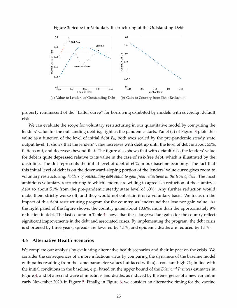
Figure 3: Scope for Voluntary Restructuring of the Outstanding Debt

(a) Value to Lenders of Outstanding Debt (b) Gain to Country from Debt Reduction

property reminiscent of the “Laffer curve” for borrowing exhibited by models with sovereign defaultrisk.

We can evaluate the scope for voluntary restructuring in our quantitative model by computing thelenders’ value for the outstanding debt B0, right as the pandemic starts. Panel (a) of Figure 3 plots thisvalue as a function of the level of initial debt B0, both axes scaled by the pre-pandemic steady stateoutput level. It shows that the lenders’ value increases with debt up until the level of debt is about 55%,flattens out, and decreases beyond that. The figure also shows that with default risk, the lenders’ valuefor debt is quite depressed relative to its value in the case of risk-free debt, which is illustrated by thedash line. The dot represents the initial level of debt of 60% in our baseline economy. The fact thatthis initial level of debt is on the downward-sloping portion of the lenders’ value curve gives room tovoluntary restructuring: holders of outstanding debt stand to gain from reductions in the level of debt. The mostambitious voluntary restructuring to which lenders are willing to agree is a reduction of the country’sdebt to about 51% from the pre-pandemic steady state level of 60%. Any further reduction wouldmake them strictly worse off, and they would not entertain it on a voluntary basis. We focus on theimpact of this debt restructuring program for the country, as lenders neither lose nor gain value. Asthe right panel of the figure shows, the country gains about 10.6%, more than the approximately 9%reduction in debt. The last column in Table 4 shows that these large welfare gains for the country reflectsignificant improvements in the debt and associated crises. By implementing the program, the debt crisisis shortened by three years, spreads are lowered by 4.1%, and epidemic deaths are reduced by 1.1%.

4.6 Alternative Health Scenarios

We complete our analysis by evaluating alternative health scenarios and their impact on the crisis. Weconsider the consequences of a more infectious virus by comparing the dynamics of the baseline modelwith paths resulting from the same parameter values but faced with a) a constant high R0 in line withthe initial conditions in the baseline, e.g., based on the upper bound of the Diamond Princess estimates inFigure 4, and b) a second wave of infections and deaths, as induced by the emergence of a new variant inearly November 2020, in Figure 5. Finally, in Figure 6, we consider an alternative timing for the vaccine

25

by pushing back its arrival by one additional year.

A highly infectious epidemic. Figure 4 documents the consequences of a permanently high level ofinfectiousness, with a fixed R0 of 2.6 throughout the pandemic. Under such a scenario, lockdownsare more intense and lengthier. Even so, the total number of eventual deaths is 4.5 times higher, withinfections spiking to well above 4.5% of the population at the peak of the episode. The intense lockdownscall for a further substantial reduction in consumption and a run-up in debt to initial output of over85%, with spreads jumping to about 12% and intense default over the following five years. Even thoughlockdowns are more intense, they are delayed and peak at the same time as infections. In preparationfor the start of these delayed lockdowns, the government reduces debt to create additional fiscal spacefor itself. This pattern illustrates the role played by time-varying R0 in our baseline parameterization: toinduce a spike in social distancing earlier than the peak of infections, as in the data.

A new variant and a second wave. As of the writing of this draft in early 2021, several countries inLatin America are experiencing a second large wave of COVID-19 cases arising from new COVID-19variants. In this section, we illustrate how our model can be used to accommodate the possibility of suchvariants. We consider the emergence of a more infectious variant of the virus, leading to a “second wave”of infections and deaths. The new variant is substantially more contagious but not inherently moredeadly, conditional on infection. It appears unexpectedly in early November and quickly becomes thepredominant source of new infections. For tractability, we do not separately keep track of the numberof infections with the new variant. Instead, we model its emergence as a spike in infectiousness bypermanently increasing R0 to 1.6, eight months after the initial outbreak. We report the dynamics of thisscenario in Figure 5.

The impact of this new variant is dramatic. A second wave of elevated daily deaths arises, spikingto 0.07 in early February 2021. At that time, over 1.6% of the population is simultaneously infected.Eventually, total deaths are slightly under 0.26% of the initial population, more than 160% of the deathsin the baseline scenario with a single outbreak. The mitigation response calls for a second lockdown,which is lengthier but less intense, as seen in panel (b) of Figure 5. This results in a 25% drop in outputat the trough and a 14% decrease in consumption shown in panels (g) and (h), respectively. Even so,the prospects of an impending vaccine induce a winding-down of social distancing measures by late2021, leading to a smaller third uptick in infections and deaths as shown in panel (d). The drop inconsumption is cushioned by additional borrowing as shown in panel (e), with debt reaching over76%. Spreads spike anew to 9.2%, as lenders price in the additional borrowing and a more protracteddebt crisis. As in the baseline, if we assume no international financial assistance and otherwise normalconditions in world financial markets, the severity of the second wave translates into a deep secondwave of a protracted debt crisis.

Delayed vaccine availability. Emerging markets face the additional hurdle of limited medical andscientific resources for managing the epidemic. As vaccines and treatments become available, accessingthese could lead to additional expenses and constraints. Our model suggests, however, that if theseinnovations become available far enough into the future, their cost and impact on the evolution of the

26

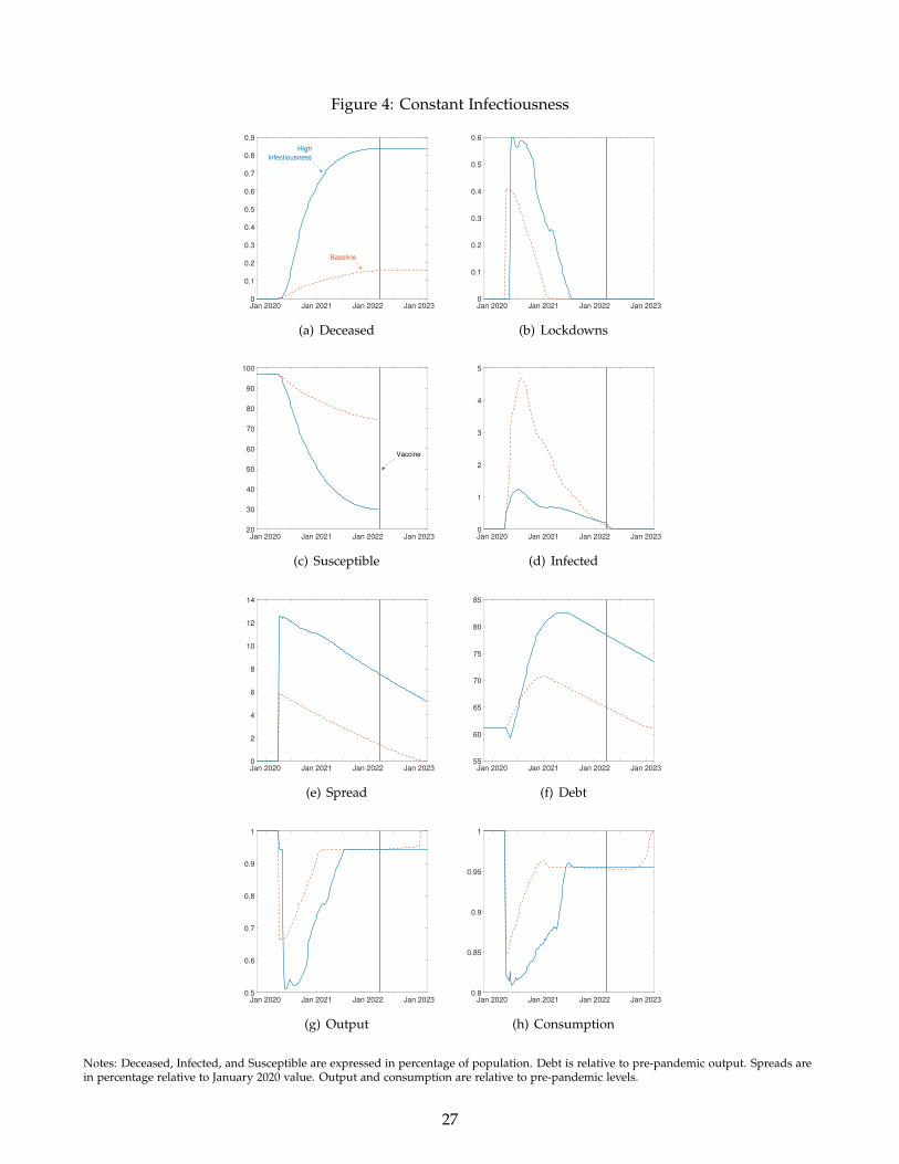
Figure 4: Constant Infectiousness

Jan 2020 Jan 2021 Jan 2022 Jan 20230

0.1

0.2

0.3

0.4

0.5

0.6

0.7

0.8

0.9

Baseline

High

Infectiousness

(a) Deceased

Jan 2020 Jan 2021 Jan 2022 Jan 20230

0.1

0.2

0.3

0.4

0.5

0.6

(b) Lockdowns

Jan 2020 Jan 2021 Jan 2022 Jan 202320

30

40

50

60

70

80

90

100

Vaccine

(c) Susceptible

Jan 2020 Jan 2021 Jan 2022 Jan 20230

1

2

3

4

5

(d) Infected

Jan 2020 Jan 2021 Jan 2022 Jan 20230

2

4

6

8

10

12

14

(e) Spread

Jan 2020 Jan 2021 Jan 2022 Jan 202355

60

65

70

75

80

85

(f) Debt

Jan 2020 Jan 2021 Jan 2022 Jan 20230.5

0.6

0.7

0.8

0.9

1

(g) Output

Jan 2020 Jan 2021 Jan 2022 Jan 20230.8

0.85

0.9

0.95

1

(h) Consumption

Notes: Deceased, Infected, and Susceptible are expressed in percentage of population. Debt is relative to pre-pandemic output. Spreads arein percentage relative to January 2020 value. Output and consumption are relative to pre-pandemic levels.

27

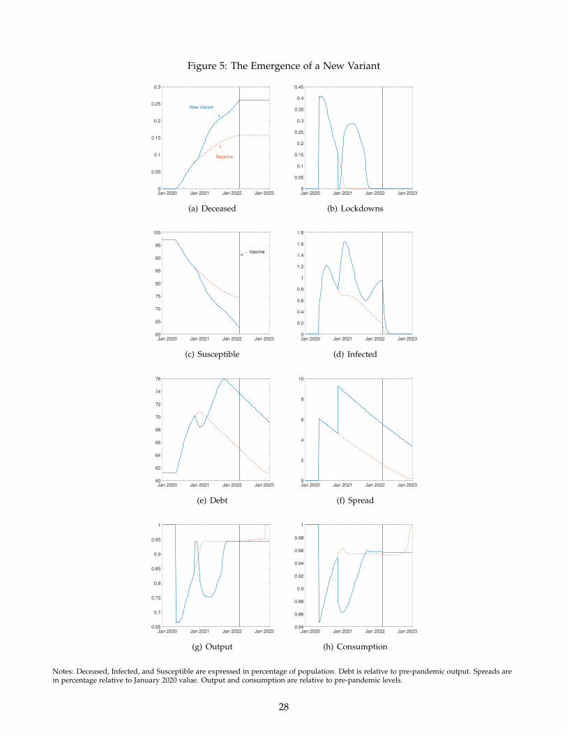
Figure 5: The Emergence of a New Variant

Jan 2020 Jan 2021 Jan 2022 Jan 20230

0.05

0.1

0.15

0.2

0.25

0.3

Baseline

New Variant

(a) Deceased

Jan 2020 Jan 2021 Jan 2022 Jan 20230

0.05

0.1

0.15

0.2

0.25

0.3

0.35

0.4

0.45

(b) Lockdowns

Jan 2020 Jan 2021 Jan 2022 Jan 202360

65

70

75

80

85

90

95

100

Vaccine

(c) Susceptible

Jan 2020 Jan 2021 Jan 2022 Jan 20230

0.2

0.4

0.6

0.8

1

1.2

1.4

1.6

1.8

(d) Infected

Jan 2020 Jan 2021 Jan 2022 Jan 202360

62

64

66

68

70

72

74

76

(e) Debt

Jan 2020 Jan 2021 Jan 2022 Jan 20230

2

4

6

8

10

(f) Spread

Jan 2020 Jan 2021 Jan 2022 Jan 20230.65

0.7

0.75

0.8

0.85

0.9

0.95

1

(g) Output

Jan 2020 Jan 2021 Jan 2022 Jan 20230.84

0.86

0.88

0.9

0.92

0.94

0.96

0.98

1

(h) Consumption

Notes: Deceased, Infected, and Susceptible are expressed in percentage of population. Debt is relative to pre-pandemic output. Spreads arein percentage relative to January 2020 value. Output and consumption are relative to pre-pandemic levels.

28

Figure 6: Later Vaccine Availability

Jan 2020 Jan 2021 Jan 2022 Jan 2023 Jan 20240

0.02

0.04

0.06

0.08

0.1

0.12

0.14

0.16

0.18

Baseline

Late Vaccine

(a) Deceased

Jan 2020 Jan 2021 Jan 2022 Jan 2023 Jan 20240

0.05

0.1

0.15

0.2

0.25

0.3

0.35

0.4

0.45

(b) Lockdowns

Jan 2020 Jan 2021 Jan 2022 Jan 2023 Jan 202470

75

80

85

90

95

100

Baseline

Vaccine

Late

Vaccine

(c) Susceptible

Jan 2020 Jan 2021 Jan 2022 Jan 2023 Jan 20240

0.2

0.4

0.6

0.8

1

1.2

1.4

(d) Infected

Jan 2020 Jan 2021 Jan 2022 Jan 2023 Jan 202460

62

64

66

68

70

72

(e) Debt

Jan 2020 Jan 2021 Jan 2022 Jan 2023 Jan 20240

1

2

3

4

5

6

(f) Spread

Jan 2020 Jan 2021 Jan 2022 Jan 2023 Jan 20240.65

0.7

0.75

0.8

0.85

0.9

0.95

1

(g) Output

Jan 2020 Jan 2021 Jan 2022 Jan 2023 Jan 20240.84

0.86

0.88

0.9

0.92

0.94

0.96

0.98

1

(h) Consumption

Notes: Deceased, Infected, and Susceptible are expressed in percentage of population. Debt is relative to pre-pandemic output. Spreads arein percentage relative to January 2020 value. Output and consumption are relative to pre-pandemic levels.

29

epidemic matter little. In Figure 6, we compare our baseline scenario with one in which the arrival ofthe vaccine is delayed by an additional year. In both scenarios, “herd immunity” is reached well inadvance of the arrival of the highly effective vaccine that quickly ends the pandemic. Even so, becauseof the longer time horizon, the scenario with a vaccine in three years after the outbreak features aneventual death toll that is higher by about 0.02% of initial population. The increase arises becausemore time before the vaccine means more opportunities for infections and also because lockdowns areendogenously slightly less aggressive as can be seen in panel (b). The associated debt crisis is slightlyless severe, as is apparent from panels (e) and (f). Panels (g) and (h) show that the impact of the timehorizon to vaccination on output and consumption is also modest, except for small timing differences inlate 2022. We conclude that the main findings of our analysis from the baseline scenario are qualitativelyand quantitatively robust to the timing of the vaccine.

5 Conclusion

We have studied the COVID-19 epidemic in emerging markets by integrating epidemiological dynamicsin a sovereign debt model and found that doing so can replicate salient features of the data on deaths,social distancing, and sovereign spreads. The pandemic is associated with many fatalities, deeprecessions, and worsened fiscal conditions, including default. With financial frictions, the death toll andseverity of the debt crisis reinforce each other as social distancing becomes increasingly costly.

By comparing our model with an otherwise equivalent one with perfect financial markets, we foundthat about a third of the welfare cost of the pandemic episode is due to default risk. Motivated bythis finding, we asked whether debt relief programs that ease financial conditions could cushion theimpact of the pandemic. We find that they deliver sizable social gains that accrue mainly to the countryand to a lesser extent to its private lenders, with no cost to financial assistance entities orchestratingthe programs. In light of these results, we find that the recent debt relief policies promoted by theInternational Monetary Fund and other international organizations are appropriate and timely forcombating the costs associated with COVID-19. We hope that our work contributes to the discussion onthe optimal domestic and international policy response to epidemic outbreaks in emerging markets.

Our results relied unavoidably on several abstractions that in turn open up promising avenues forsubsequent work. We did not address the decentralization of optimal lockdowns in our model and therelated question of whether the private sector alone would under- or over-provide social distancing.Note that in our setting, the private sector could depress activity excessively, as it may not internalize theeffects on the fiscal conditions of the sovereign, including the resulting debt crisis. This stands in contrastwith the better-understood externality whereby the private sector does not social distance enough, asagents do not internalize the role they might play in contagion and deaths in the broader economy.Finally, we conjecture that the mechanism we explored, relating financial conditions to mitigation efforts,could also operate at the individual level. For example, wealthier and financially unconstrained agentsmight lock down and isolate more aggressively, while agents unable to smooth consumption throughborrowing might choose to expose themselves and others to increased risk. We further suspect that sucha cross-sectional pattern would be salient not only in emerging markets but in advanced economies aswell.

30

References

Acemoglu, Daron, Victor Chernozhukov, Ivan Werning, and Michael D Whinston. 2020. Optimal TargetedLockdowns in a Multi-Group SIR Model. Working Paper 27102. National Bureau of Economic Research,May. https://doi.org/10.3386/w27102. http://www.nber.org/papers/w27102.

Aguiar, Mark, and Manuel Amador. 2011. “Growth in the Shadow of Expropriation.” The QuarterlyJournal of Economics 126, no. 2 (June): 651–697.

Aguiar, Mark, Manuel Amador, Hugo Hopenhayn, and Ivan Werning. 2019. “Take the short route:Equilibrium default and debt maturity.” Econometrica 87 (2): 423–462.

Aguiar, Mark, and Gita Gopinath. 2006. “Defaultable debt, interest rates and the current account.” Journalof International Economics 69, no. 1 (June): 64–83.

Cakmaklı, Cem, Selva Demiralp, Sebnem Kalemli-Ozcan, Sevcan Yesiltas, and Muhammed A Yildirim.2020. COVID-19 and Emerging Markets: A SIR Model, Demand Shocks and Capital Flows. WorkingPaper 27191. National Bureau of Economic Research, May. https://doi.org/10.3386/w27191.http://www.nber.org/papers/w27191.

Alvarez, Fernando E, David Argente, and Francesco Lippi. 2020. A Simple Planning Problem for COVID-19Lockdown. Working Paper 26981. National Bureau of Economic Research, April. https://doi.org/10.3386/w26981. http://www.nber.org/papers/w26981.

Arellano, Cristina. 2008. “Default risk and income fluctuations in emerging economies.” AmericanEconomic Review 98 (3): 690–712.

Arellano, Cristina, Yan Bai, and Gabriel P Mihalache. 2020. Monetary Policy and Sovereign Risk in EmergingEconomies (NK-Default). Working Paper 26671. National Bureau of Economic Research, January.https://doi.org/10.3386/w26671. http://www.nber.org/papers/w26671.

Arellano, Cristina, Xavier Mateos-Planas, and Jose-Vıctor Rıos-Rull. 2019. Partial Default. WorkingPaper 26076. National Bureau of Economic Research, June. https://doi.org/10.3386/w26076.http://www.nber.org/papers/w26076.

Atkeson, Andrew. 2020. What Will Be the Economic Impact of COVID-19 in the US? Rough Estimates ofDisease Scenarios. Working Paper 26867. National Bureau of Economic Research, March. https ://doi.org/10.3386/w26867. http://www.nber.org/papers/w26867.

Atkeson, Andrew, Karen Kopecky, and Tao Zha. 2020. Estimating and Forecasting Disease Scenarios forCOVID-19 with an SIR Model. Working Paper 27335. National Bureau of Economic Research, June.https://doi.org/10.3386/w27335. http://www.nber.org/papers/w27335.

Azzimonti, Marina, Alessandra Fogli, Fabrizio Perri, and Mark Ponder. 2020. Pandemic Control inECON-EPI Networks. Working Paper 27741. National Bureau of Economic Research, August. https://doi.org/10.3386/w27741. http://www.nber.org/papers/w27741.

31

Baqaee, David, Emmanuel Farhi, Michael J Mina, and James H Stock. 2020. Reopening Scenarios. WorkingPaper 27244. National Bureau of Economic Research, May. https://doi.org/10.3386/w27244.http://www.nber.org/papers/w27244.

Bulow, Jeremy, and Kenneth Rogoff. 1988. “The buyback boondoggle.” Brookings Papers on EconomicActivity 1988 (2): 675–704.

Chatterjee, Satyajit, and Burcu Eyigungor. 2012. “Maturity, indebtedness, and default risk.” AmericanEconomic Review 102 (6): 2674–2699.

Cruces, Juan J., and Christoph Trebesch. 2013. “Sovereign Defaults: The Price of Haircuts.” AmericanEconomic Journal: Macroeconomics 5, no. 3 (June): 85–117.

Dingel, Jonathan I, and Brent Neiman. 2020. “How many jobs can be done at home?” Journal of PublicEconomics 189:104235.

Dvorkin, Maximiliano, Juan M. Sanchez, Horacio Sapriza, and Emircan Yurdagul. 2018. Sovereign DebtRestructurings. Working Papers 2018-13. Federal Reserve Bank of St. Louis, June. https://ideas.repec.org/p/fip/fedlwp/2018-013.html.

Eaton, Jonathan, and Mark Gersovitz. 1981. “Debt with Potential Repudiation: Theoretical and EmpiricalAnalysis.” Review of Economic Studies 48 (2): 289–309.

Eichenbaum, Martin S, Sergio Rebelo, and Mathias Trabandt. 2020. The Macroeconomics of Epidemics.Working Paper 26882. National Bureau of Economic Research, March. https://doi.org/10.3386/w26882. http://www.nber.org/papers/w26882.

Espino, Emilio, Julian Kozlowski, Fernando M. Martin, and Juan M. Sanchez. 2020. Seigniorage andSovereign Default: The Response of Emerging Markets to COVID-19. Working Papers 2020-017. FederalReserve Bank of St. Louis, July. https://doi.org/10.20955/wp.2020.017. https://ideas.repec.org/p/fip/fedlwp/88355.html.

Farboodi, Maryam, Gregor Jarosch, and Robert Shimer. 2020. Internal and External Effects of SocialDistancing in a Pandemic. Working Paper 27059. National Bureau of Economic Research, April.https://doi.org/10.3386/w27059. http://www.nber.org/papers/w27059.

Global Financial Data. 2021. “JP Morgan EMBI+.” https://globalfinancialdata.com/.

Glover, Andrew, Jonathan Heathcote, Dirk Krueger, and Jose-Vıctor Rıos-Rull. 2020. Health versus Wealth:On the Distributional Effects of Controlling a Pandemic. Working Paper 27046. National Bureau ofEconomic Research, April. https://doi.org/10.3386/w27046. http://www.nber.org/papers/w27046.

Google LLC. 2021. “Google COVID-19 Community Mobility Reports.” https://www.google.com/covid19/mobility/.

Gordon, Grey. 2019. Efficient Computation with Taste Shocks. Working Paper 19-15. Federal Reserve Bankof Richmond, September. https://ideas.repec.org/p/fip/fedrwp/19-15.html.

32

Gourinchas, Pierre-Olivier, and Chang-Tai Hsieh. 2020. “The COVID 19 Default Time Bomb.” ProjectSyndicate, April. https://www.project-syndicate.org/commentary/covid19-sovereign-default-time-bomb-by-pierre-olivier-gourinchas-and-chang-tai-hsieh-2020-04.

Guerrieri, Veronica, Guido Lorenzoni, Ludwig Straub, and Ivan Werning. 2020. Macroeconomic Implicationsof COVID-19: Can Negative Supply Shocks Cause Demand Shortages? Working Paper 26918. NationalBureau of Economic Research. https://doi.org/10.3386/w26918. http://www.nber.org/papers/w26918.

Hatchondo, Juan C, Leonardo Martinez, and Cesar Sosa-Padilla. 2014. “Voluntary sovereign debtexchanges.” Carnegie-Rochester-NYU Conference Series on ‘Fiscal Policy in the Presence of DebtCrises’ held at the Stern School of Business, New York University on April 19-20, 2013, Journal ofMonetary Economics 61:32–50. issn: 0304-3932. https://doi.org/10.1016/j.jmoneco.2013.11.002.https://www.sciencedirect.com/science/article/pii/S0304393213001487.

. 2020. Sovereign Debt Standstills. Working Paper 28292. National Bureau of Economic Research,December. https://doi.org/10.3386/w28292. http://www.nber.org/papers/w28292.

Hatchondo, Juan Carlos, and Leonardo Martinez. 2009. “Long-duration bonds and sovereign defaults.”Journal of International Economics 79 (1): 117 –125. issn: 0022-1996. https://doi.org/10.1016/j.jinteco.2009.07.002. http://www.sciencedirect.com/science/article/pii/S0022199609000907.

Hatchondo, Juan Carlos, Leonardo Martinez, and Yasin Kursat Onder. 2017. “Non-defaultable debt andsovereign risk.” Journal of International Economics 105:217–229. issn: 0022-1996. https://doi.org/10.1016/j.jinteco.2017.01.008. https://www.sciencedirect.com/science/article/pii/S0022199617300107.

Hethcote, Herbert W. 2000. “The mathematics of infectious diseases.” SIAM review 42 (4): 599–653.

Hevia, Constantino, and Andy Neumeyer. 2020. A Conceptual Framework for Analyzing the EconomicImpact of COVID-19 and its Policy Implications. Technical report, Policy Document Series. UNDP LatinAmerican and the Cribbean.

Kermack, William Ogilvy, and Anderson G McKendrick. 1927. “A contribution to the mathematical the-ory of epidemics.” Proceedings of the royal society of london. Series A, Containing papers of a mathematicaland physical character 115 (772): 700–721.

Moll, Benjamin. 2020. Lockdowns in SIR Models. Technical report. Lecture Notes, Princeton University.

Mossong, Joel, Niel Hens, Mark Jit, Philippe Beutels, Kari Auranen, Rafael Mikolajczyk, Marco Massari,et al. 2008. “Social Contacts and Mixing Patterns Relevant to the Spread of Infectious Diseases.”PLOS Medicine 5, no. 3 (March): 1–1. https://doi.org/10.1371/journal.pmed.0050074. 10.1371/journal.pmed.0050074.

Saltiel, Fernando. 2020. “Who can work from home in developing countries.” Covid Economics 7 (2020):104–118.

Thomas, Jonathan, and Tim Worrall. 1994. “Foreign direct investment and the risk of expropriation.” TheReview of Economic Studies 61 (1): 81–108.

33

Viscusi, W. Kip, and Clayton J. Masterman. 2017. “Income Elasticities and Global Values of a StatisticalLife.” Journal of Benefit-Cost Analysis 8, no. 2 (July): 226–250. https://ideas.repec.org/a/cup/jbcoan/v8y2017i02p226-250 00.html.

Wang, Huwen, Zezhou Wang, Yinqiao Dong, Ruijie Chang, Chen Xu, Xiaoyue Yu, Shuxian Zhang, et al.2020. “Phase-adjusted estimation of the number of coronavirus disease 2019 cases in Wuhan, China.”Cell Discovery 6 (1): 1–8.

worldometers.info. 2021. “COVID-19 Data.” https://www.worldometers.info/.

Zhang, Sheng, MengYuan Diao, Wenbo Yu, Lei Pei, Zhaofen Lin, and Dechang Chen. 2020. “Estimationof the reproductive number of novel coronavirus (COVID-19) and the probable outbreak size onthe Diamond Princess cruise ship: A data-driven analysis.” International Journal of Infectious Diseases93:201–204.

34

Online Appendix to

“Deadly Debt Crises: COVID-19 in Emerging Markets”

by Cristina Arellano, Yan Bai, and Gabriel Mihalache

A Recursive Formulation before the Epidemic

The recursive problem for the government before the epidemic resembles the one in Arellano, Mateos-Planas, and Rıos-Rull (2019). We assume that the government does not expect the epidemic to arise inthe future, the probability of dying is expected to always be zero, and the measure of total populationremains at one throughout. We study a Markov problem for the government. In period t, with debtholding Bt, the government chooses new issuance `t and partial default intensity dt ∈ [0, 1] to solve

Vpre (Bt) = max`t, dt∈[0,1]

u(ct) + βVpre (Bt+1) , (24)

subject to the evolution of the debt in equation (4), the resource constraint of the economy (3) withNt = 1, and the bond price function qpre(Bt+1). The Markov structure generates a time-invariant bondprice schedule that depends on future default and borrowing decisions:

qpre(Bt+1) =1

1 + r{(δ + r)(1− dt+1(Bt+1)) + [1− δ + κ(δ + r)dt+1(Bt+1)] qpre(Bt+2(Bt+1))} . (25)

This problem induces in pre-epidemic decision rules for the evolution of government debt Bt+1 =

Bpre(Bt), default dt = dpre(Bt), and per capita consumption ct = cpre(Bt). It also delivers the bond priceschedule qpre(Bt+1) and value function Vpre (Bt). We use these results to set terminal conditions for thefollowing problem during the epidemic. In the baseline experiment, we use the steady state values fordebt Bt from this problem as its initial condition.

B Definition of Epidemic Equilibrium

The epidemic equilibrium consists of sequences of functions for consumption ct(µt, Bt), the government’sborrowing policy Bt+1(µt, Bt), default dt(µt, Bt), and lockdown Lt(µt, Bt); the value function Vt(µt, Bt);the bond price schedule qt(µt, Bt+1); and the epidemiological laws of motion µt+1(µt, Bt) that summarizesthe mass of susceptible, infected, and recovered for period t = 0, 1, 2, ... such that, given the initial state(µ0, B0) and the availability of the vaccine in period H,

(i) For periods t > H, the epidemic is eliminated, µSt = 0, µI

t = 0, and µRt = µR

H + µSH +(1−π0

D/πI)µIH

under the assumption that at period H, a fraction π0D/πI of the infected dies and the rest recover.

The optimal lockdown intensity is zero, Lt(µt, Bt) = 0. The government’s borrowing and defaultpolicies, the value function, and the bond price schedule are the same as the pre-epidemicones, Vt(µt, Bt) = Vpre(Bt), dt(µt, Bt) = dpre(Bt), Bt+1(µt, Bt) = Bpre(µt, Bt), and qt(µt, Bt+1) =

qpre(Bt+1).

A1

(ii) For any period t ≤ H, taking as given the value function and the bond price schedule for periodt + 1, the government’s value function and policies solve

Vt (µt, Bt) = maxBt+1, dt∈[0,1], Lt∈[0,1]

[u(ct)− χφD,t] + βVt+1 (µt+1(µt, Lt), Bt+1) ,

subject to the resource constraint

Ntct + (1− dt)(δ + r)Bt =zφ(dt)Nt(1− Lt) + qt(µt+1(µt, Lt), Bt+1)(Bt+1 − (1− δ)Bt),

the SIR laws of motion (6)-(9), deaths φD,t = πD(µIt )µ

It for t < H and φD,t = π0

D/πIµIt for t = H,

and Nt = µSt + µI

t + µRt .

(iii) For any period t ≤ H, taking as given the government’s policies in period t + 1 and the epidemio-logical state, the bond price schedule satisfies

qt(µt+1(µt, Lt), Bt+1) =1

1 + r{(δ + r)(1− dt+1) + [1− δ + κ(δ + r)dt+1] qt+1(µt+2, Bt+2)} .

(iv) The evolution of the epidemiological state µt+1(µt, Bt) is consistent with the SIR laws of motion(6)-(9) and equilibrium social distancing Lt = Lt(µt, Bt).

C Reference Models

Perfect financial markets. In period 0, the government chooses sequences of consumption {ct} andlockdowns {Lt}, with Lt ∈ [0, 1], to maximize its lifetime value (1), subject to the lifetime budgetconstraint

∞

∑t=0

1(1 + r)t Ntct =

∞

∑t=0

1(1 + r)t z[Nt(1− Lt)]

α, (26)

the SIR laws of motion (6)-(9) and the total population constraint (11). For an initial debt level B0, weback out long-term borrowing, with the same maturity structure as in the baseline, recursively from theper-period budget constraints, using the optimal allocations, lockdowns, and SIR dynamics, for any t:

q f Bt+1 = Ntct + [(δ + r) + q f (1− δ)]Bt + z[Nt(1− Lt)]α,

where the risk-free, long-term bond price q f satisfies

q f =1

1 + r[(δ + r) + (1− δ)q f ].

Because of our choice of normalization for the payments scheduled by each unit of debt, we have q f = 1.As pre-pandemic steady state output in weeks is 1, we can interpret Bt not only as abstract bond unitsbut also as multiple of weekly output; thus, a Bt of 52 would imply a debt-to-output ratio of 100%.

Financial autarky. In this model, the government cannot borrow or lend internationally. It choosesconsumption and lockdown to maximize its lifetime value (1), subject to period-by-period budget

A2

constraints,

Ntct =z[Nt(1− Lt)]α; (27)

the SIR lows of motion (6)-(9), and the total population constraint (11).

D Proofs

Before proceeding to the proofs of propositions 1 and 2, we first set up the stripped-down, two-periodversion of the model from Section 3. The economy starts with zero debt B0 = 0 and population N0, whichconsists of measure µS

0 susceptible, µI0 infected, and µR

0 recovered individuals; that is, N0 = µS0 + µI

0 + µR0 .

In the last period, period 1, the government cannot issue more debt, B2 = 0.The government has limited commitment and can choose to default on its debt. With zero initial debt,

the government will not default in period 0. It chooses consumption (c0, c1) and lockdowns (L0, L1) inboth periods and borrowing B1 and partial default d1 ∈ [0, 1] in period 1 to maximize its objective

max [u(c0)− χφD,0] + β [u(c1)− χφD,1(L0)] , (28)

subject to the budget constraints of each period,

N0c0 = zN0(1− L0) + q0(B1)B1,

N1c1 + (1− d1)B1 = zγ(d1)N1(1− L1);

the evolution of infected, susceptible, and recovered

µI1(L0) = πIµ

I0 + πSI(1− θL0)

2µI0µS

0 , (29)

µS1(L0) = µS

0 − πSI(1− θL0)2µI

0µS0 , (30)

µR1 = µR

0 + (1− πI)µI0 − φD,0; (31)

the fatalities induced by infection

φD,1(L0) = πD(µI1(L0))µ

I1(L0); (32)

the evolution of total populationN1 = N0 − φD,0; (33)

and the bond price scheduleq0(B1) = (1− d1(B1))/(1 + r). (34)

It is easy to see that the government will not impose any lockdown in the last period, L1 = 0, sincedoing so does not affect the spread of the disease and death. The government also cannot influence thedeath toll in period 0, φD,0, nor can it influence the total population in period 1, N1. Given that both φD,0

and N1 are determined by the initial level of infection and epidemiology parameters, we assume for

A3

simplicity that φD,0 = 0.In the stripped-down version of the model, we make the following assumptions to guarantee interior

solutions to partial default d1 ∈ [0, 1] and lockdown L0 ∈ [0, 1] to better illustrate the interactionmechanism between the health and debt crisis. These assumptions are relaxed in the general model.

Assumptions

1. The discount factor is such that β(1 + r) ≤ 1. The lockdown effectiveness takes the value of 1,θ = 1. The case fatality rate is constant, πD(µ

I0) = π0

D. The value of life χ satisfies

χ ≥ z1−σ

2βπ0DπSIµ

I0µS

0

(1 +

11 + r

)−σ

λ−σ,

where λ =[1 + β

1σ (1 + r)

1−σσ

]−1< 1.

2. The function γ : [0, 1]→ R is differentiable, decreasing γ′ < 0, concave γ′′ < 0, and with γ(0) = 1and γ′(0) = 0.

3. Let d be the maxima of the function f (d) = −(1− d)γ′(d). We assume f (d) ≥ λ.

Note that Assumption 2 implies γ′(d), and so f (d) are continuous functions. By the maximumtheorem, there exists a d ∈ [0, 1] that maximizes the f function. Furthermore, f (0) = f (1) = 0, sinceγ′(0) = 0. It has to be the case that 0 < d < 1.19

D.1 Proof of Proposition 1

Proof. We start with the baseline’s equilibrium conditions under the assumption of interior solutionsfor default and lockdown. We then verify that Assumptions 1-3 guarantee that the solution is indeedinterior. The equilibrium default, borrowing, consumption, and lockdown, {d1, B1, c1, c0, L0}, satisfy thefollowing five equations:

−zγ′(d1)N1 = B1, (35)

u′(c0) = β(1 + rd(B1))u′(c1), (36)

N1c1 + (1− d1)B1 = zγ(d1)N1, (37)

c0 =1

1 + 11+r [β(1 + rd(B1))]1/σ

(z(1− L0) +

11 + r

zγ(d1)

), (38)

zu′(c0) = βχ

(−∂φD,1(L0)

∂L0

), (39)

where 1 + rd(B1) = (1 + r)/(1− η(B1)) is the domestic interest rate, with η(B1) defined as the elasticityof bond price with respect to borrowing η(B1) = −∂ ln(q0)/∂ ln(B1) ≥ 0. Equation (35) is the first ordercondition on partial default d1 in period 1; equation (36) is the Euler equation for borrowing B1; equation

19. An example of γ function satisfying assumptions 2 and 3 is γ(d) = 1− γ0dγ1 with γ1 > 1 and γ0 ≥ λ((γ1 − 1)/γ1)1−γ1 .

In this case, γ′(d) < 0, γ′′(d) < 0, γ(0) = 1, and γ′(0) = 0. The maxima is d = (γ1 − 1)/γ1 with 0 < d < 1. At the maxima,f (d) ≤ λ, since γ0 ≥ λ((γ1 − 1)/γ1)

1−γ1 .

A4

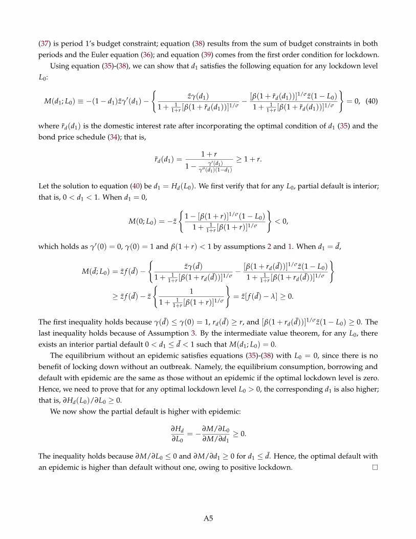
(37) is period 1’s budget constraint; equation (38) results from the sum of budget constraints in bothperiods and the Euler equation (36); and equation (39) comes from the first order condition for lockdown.

Using equation (35)-(38), we can show that d1 satisfies the following equation for any lockdown levelL0:

M(d1; L0) ≡ −(1− d1)zγ′(d1)−{

zγ(d1)

1 + 11+r [β(1 + rd(d1))]1/σ

− [β(1 + rd(d1))]1/σ z(1− L0)

1 + 11+r [β(1 + rd(d1))]1/σ

}= 0, (40)

where rd(d1) is the domestic interest rate after incorporating the optimal condition of d1 (35) and thebond price schedule (34); that is,

rd(d1) =1 + r

1− γ′(d1)γ′′(d1)(1−d1)

≥ 1 + r.

Let the solution to equation (40) be d1 = Hd(L0). We first verify that for any L0, partial default is interior;that is, 0 < d1 < 1. When d1 = 0,

M(0; L0) = −z

{1− [β(1 + r)]1/σ(1− L0)

1 + 11+r [β(1 + r)]1/σ

}< 0,

which holds as γ′(0) = 0, γ(0) = 1 and β(1 + r) < 1 by assumptions 2 and 1. When d1 = d,

M(d; L0) = z f (d)−{

zγ(d)1 + 1

1+r [β(1 + rd(d))]1/σ− [β(1 + rd(d))]1/σ z(1− L0)

1 + 11+r [β(1 + rd(d))]1/σ

}

≥ z f (d)− z

{1

1 + 11+r [β(1 + r)]1/σ

}= z[ f (d)− λ] ≥ 0.

The first inequality holds because γ(d) ≤ γ(0) = 1, rd(d) ≥ r, and [β(1 + rd(d))]1/σ z(1− L0) ≥ 0. Thelast inequality holds because of Assumption 3. By the intermediate value theorem, for any L0, thereexists an interior partial default 0 < d1 ≤ d < 1 such that M(d1; L0) = 0.

The equilibrium without an epidemic satisfies equations (35)-(38) with L0 = 0, since there is nobenefit of locking down without an outbreak. Namely, the equilibrium consumption, borrowing anddefault with epidemic are the same as those without an epidemic if the optimal lockdown level is zero.Hence, we need to prove that for any optimal lockdown level L0 > 0, the corresponding d1 is also higher;that is, ∂Hd(L0)/∂L0 ≥ 0.

We now show the partial default is higher with epidemic:

∂Hd

∂L0= −∂M/∂L0

∂M/∂d1≥ 0.

The inequality holds because ∂M/∂L0 ≤ 0 and ∂M/∂d1 ≥ 0 for d1 ≤ d. Hence, the optimal default withan epidemic is higher than default without one, owing to positive lockdown.

A5

D.2 Proof of Proposition 2

Proof. Under perfect financial markets, the government commits to repay its debt and chooses con-sumption (c0, c1) and lockdown (L0, L1) to maximize its objective (28), subject to the lifetime budgetconstraint

N0c0 +1

1 + rN1c1 = zN0(1− L0) +

11 + r

zN1(1− L1),

fatalities (32), SIR laws of motion (29)-(31), and the evolution of population (33). Recall that we assumeφD,0 = 0, and so N1 = N0. In this case, we can back up the optimal borrowing from period 0’s budgetconstraint B1 = (1 + r)[N0c0 − zN0(1− L0)]. Let the optimal consumption and lockdown under perfectfinancial markets be (ce

0, ce1, Le

0). Similarly, as in (38) in the baseline, consumption c0 is a share of thelifetime income:

ce0 =

11 + 1

1+r [β(1 + r)]1/σ

(z(1− Le

0) +1

1 + rz)

.

The optimal lockdown Le0 weights the marginal benefit and cost as in (39). Plugging in the optimal

consumption ce0 into (39), we find the equation characterizing optimal lockdown under perfect financial

markets: (z(1− L0) +

11+r z

1 + 11+r [β(1 + r)]1/σ

)−σ

z = 2βχπ0DπSIµ

I0µS

0(1− L0), (41)

where the right-hand side is the marginal benefit of lockdown—that is, βχ(− ∂φD,1(L0)

∂L0

). According to

Assumption 1, the left-hand side is lower than the right-hand side when L0 = 0, and the left-hand sideis higher than the right-hand side when L0 = 1. Hence, by the intermediate value theorem, the optimalLe

0 is between 0 and 1.Similarly, plugging in the consumption (38) and default intensity (35) into the first order condition

for lockdown (39), we can show that the optimal lockdown in our baseline satisfies(z(1− L0) +

11+r zγ(d1)

1 + 11+r [β(1 + rd(d1))]1/σ

)−σ

z = 2βχπ0DπSIµ

I0µS

0(1− L0). (42)

As in the perfect financial markets case, there is an interior solution for lockdown. It is easy to showthat under d1 = 0, the optimal lockdown in our baseline is the same as the one from perfect financialmarkets Le

0. However, with d1 > 0, for the same level of L0, the left-hand side of (42) becomes largerthan that of (41) owing to both lower γ(d1) and a higher domestic interest rate rd(d1) in the baselinemodel. Hence the marginal benefit of locking down is smaller as long as d1 > 0, which leads to a lowerlockdown level than Le

0. In summary, the lockdown level in our baseline is equal to or lower than Le0.

With lower lockdown, the death toll φD,1 is higher in our baseline model.

E Computational Algorithm

In this appendix, we describe the computation of our model. We augment the original problem withtaste shocks on debt choices B′, following Dvorkin, Sanchez, Sapriza, and Yurdagul (2018) and Gordon

A6

(2019), and then we describe the computation algorithm, which solves backwards in time for value andpolicy functions.

The taste shock on B′ helps numerical stability and the convergence properties of our model withlong-term, defaultable debt. The set of B is discrete, and each element in the set is associated with an iidtaste shock, distributed Gumbel (Extreme Value Type I). The parameter controlling the magnitude oftaste shocks is ρB.

Model with taste shocks. For the purposes of this appendix, we switch the state from (µSt , µI

t , µRt ), the

one in the main text, to (µSt , µI

t , µDt ). Given that the sum of the four group is always 1, µS

t +µIt +µR

t +µDt =

1, the two formulations are equivalent. With slight abuse of notation, we use µt = (µSt , µI

t , µDt ) as the SIR

state variable. The government’s problem becomes

Wt (µt, Bt, Bt+1) = maxLt,dt

u(ct)− πD(µIt )µ

It + βVt+1 (µt+1(µt, Lt), Bt+1) , (43)

subject to the resource constraint and the SIR laws of motion

ct = zφ(dt)(1− Lt) +{Bt+1 − [1− δ + κ(δ + r)dt] Bt} qt(µt+1(µt, Lt), Bt+1)− (δ + r)(1− dt)Bt

1− µDt

(44)

µxt = πSI(1− θLt)

2µSt µI

t (45)

µSt+1 = µS

t − µxt (46)

µIt+1 = πIµ

It + µx

t (47)

µDt+1 = µD

t + πD(µIt )µ

It . (48)

Let the optimal default and lockdown choices be dt(µt, Bt, Bt+1) and Lt(µt, Bt, Bt+1), respectively. Thechoice probabilities over Bt+1 are given by

Pr (Bt+1|µt, Bt) =exp((Wt(µt, Bt, Bt+1)−Wt(µt, Bt))/ρB)

∑Bt+1exp((Wt(µt, Bt, Bt+1)−Wt(µt, Bt))/ρB)

,

where W is the maximum option net of taste shocks, Wt(µt, Bt) = maxBt+1 Wt(µt, Bt, Bt+1). The value V,in expectation over taste shocks, satisfies

Vt(µt, Bt) = Wt(µt, Bt) + ρB log

{∑Bt+1

expWt(µt, Bt, Bt+1)−Wt(µt, Bt)

ρB

}.

We write the bond price schedule for any choices (Lt, Bt+1) in state µt as

qt (µt+1, Bt+1) =1

1 + r ∑Bt+2

Pr (Bt+2|µt+1, Bt+1)×

{(δ + r)(1− d∗t+1) + [1− δ + κ(δ + r)d∗t+1] qt+1 (µt+2(µt+1, L∗t+1), Bt+2)} ,

A7

where d∗t+1 = dt+1(µt+1, Bt+1, Bt+2) and L∗t+1 = Lt+1(µt+1, Bt+1, Bt+2) and equilibrium policies evaluateat the relevant future state.

Computational algorithm. Note that in period t, the state variable µDt affects the period t allocation

only through the per-capita debt burden Bt/(1− µDt ) and per-capita borrowing Bt+1/(1− µD

t ). Inparticular, µD

t does not affect current or future losses from death. At our benchmark SIR parameters, theeventual death toll is less than 1% without lockdowns, and hence its impact on per capita debt is small.Therefore, we approximate the original problem with a simplified one with SIR state variables restrictedto (µS

t , µIt ) and rewrite the resource constraint as

ct = zφ(dt)(1− Lt)α + {Bt+1 − [1− δ + κ(δ + r)dt] Bt} qt(µt+1(µt, Lt), Bt+1)− (δ + r)(1− dt)Bt. (49)

We verified that the simplified problem approximates well the original one. This simplification, however,reduces the state space by one variable and dramatically saves computation time.

We first solve the stationary equilibrium, which both is the solution for the pre-epidemic equilibriumand governs behavior after the introduction of the vaccine. We then solve backwards over time theequilibrium under SIR dynamics.

1. Stationary equilibrium

(a) Guess value function Vs(B) and bond price schedule qs(B′).

(b) For each (B, B′), solve for the optimal default decision. We find the solution d∗ of the followingfirst order condition for partial default,

−zφ′(d) = (δ + r)B[1− κqs(B′)

].

Evaluate the consumption per capita c from the resource constraint

c = zφ(d) +{

B′ − [1− δ + κ(δ + r)d] B}

qs(B′)− (δ + r)(1− d)B

at three default choice levels, d = {d∗, 0, 1}, and pick the default intensity that results in thehighest consumption per capita under (B, B′). Let the optimal default be ds(B, B′) and thecorresponding consumption be cs(B, B′).

(c) Compute the value from (B, B′) and the optimal default intensity ds(B, B′). Then, we evaluateWs (B, B′) = u(cs(B, B′)) + βVs (B′).

(d) Calculate the probability of each B′,

Pr(

B′|B)=

exp((Ws(B, B′)−Ws(B))/ρB)

∑B′ exp((Ws(B, B′)−Ws(B))/ρB)

,

and the maximum Ws for each b, Ws(B) = maxB′ Ws(B, B′).

(e) Update Vs(B), Vs(B) = Ws(B) + ρB log

{∑B′ exp Ws(B,B′)−Ws

(B)ρB

}.

A8

(f) Update the bond price schedule qs(B′),

qs (B′) = 11 + r ∑

B′′Pr(

B′′|B′) {

(δ + r)(1− d(B′, B′′)) +[1− δ + κ(δ + r)ds(B′, B′′)

]qs (B′′)} .

(g) Check whether Vs and qs converged. If both did, we are done. Otherwise, go back to step1(b).

2. Period H problem (with vaccine)In period H, a vaccine is available. All susceptible individuals are marked as recovered; a fractionπ0

D/πI of the infected dies, while the rest recover:

WH (µH, BH, BH+1) = maxdH

{u(cH)−

[π0

DπI

]µI

Hχ + βVs (BH+1)

}, (50)

subject to the resource constraint (49). Let the solution be V{0}H (µH, BH), d{0}H (µH, BH, BH+1),Pr{0} (BH+1|µH, BH), q{0}H (µH+1, BH+1), and L{0}H (µH, BH, BH+1) = 0.

3. Period t < H problem

(a) Start with q{0}t+1(µt+2, Bt+2), d0t+1(µt+1, Bt+1, Bt+2), L0

t+1(µt+1, Bt+1, Bt+2), Pr{0} (Bt+2|µt+1, Bt+1),and V{0}t+1 (µt+1, Bt+1).

(b) Construct bond price q{1}t (µt+1, Bt+1):

q{1}t (µt+1, Bt+1) =1

1 + r ∑Bt+2

Pr{0} (Bt+2|µt+1, Bt+1){(δ + r)(1− d{0}t+1)

+[1− δ + κ(δ + r)d{0}t+1

]q{0}t+1

(µt+2(µt+1, L{0}t+1), Bt+2

) },

where d{0}t+1 = d{0}t+1(µt+1, Bt+1, Bt+2) and L{0}t+1 = L{0}t+1(µt+1, Bt+1, Bt+2).

(c) Solve for the optimal default and lockdown policies for each Bt and Bt+1 paid,

Wt (µt, Bt, Bt+1) = maxLt,dt

u(ct)− πD(µIt )µ

It χ + βV{0}t+1 (µt+1(µt, Lt), Bt+1) ,

subject to the resource constraint (49) and the SIR laws of motion. Specifically, we search overthe grid of Lt. For each (µt, Bt, Bt+1, Lt), we find the solution d∗ to the following equation:

−zφ′(d)(1− Lt)α(1− µD

t ) = (δ + r)Bt

[1− κq{1}t (µt+1(µt, Lt), Bt+1)

].

We pick the default choice in {d∗, 0, 1} which yields the highest consumption per capitafor (µt, Bt, Bt+1, Lt). Let the optimal default and lockdown choices be d{1}t (µt, Bt, Bt+1) andL{1}t (µt, Bt, Bt+1).

(d) Calculate the probability of choosing each Bt+1:

Pr{1} (Bt+1|µt, Bt) =exp((Wt(µt, Bt, Bt+1)−Wt(µt, Bt))/ρB)

∑Bt+1exp((Wt(µt, Bt, Bt+1)−Wt(µt, Bt))/ρB)

,

A9

with the maximum value given by Wt(µt, Bt) = maxBt+1 Wt(µt, Bt, Bt+1).

(e) Calculate the period t’s value and bond price functions, for use at t− 1:

V{1}t (µt, Bt) = Wt(µt, Bt) + ρB log

{∑Bt+1

expWt(µt, Bt, Bt+1)−Wt(µt, Bt)

ρB

}.

(f) Assign the functions with superscript {1} to functions with superscript {0}. Go back to step3(a) for the previous t until t = 0, then stop.

A10