Decentralized Industrial Policy

Wei Chen, Ernest Liu, Zheng (Michael) Song

Abstract

Many industrial policies were enacted by local governments. Decentralizing governmentintervention can undermine industrial policies if the local and aggregate welfares are mis-aligned. In this paper, we extend the closed-economy analysis in Liu (2019) to a multi-regionsetting with inter-regional trade and input-output linkages. We derive sucient statistics forthe regional and aggregate welfare impacts of industrial policy. Using China’s cross-provinceinput-output table, we show there is signicant divergence between the incentives of thecentral and a provincial government: while the nation may benet from promoting upstreamsectors, regional economies benet from “import substitution” policies that improve terms-of-trade but may harm the nation. Our central and local sucient statistics predict policiesenacted by the respective governments. The predictive power for local industrial policies im-proves in the regions with more scal autonomy. Adopting industrial policies aligned withcentral sucient statistics can double the aggregate welfare gain by industrial policies alignedwith local sucient statistics.

1

1 Introduction

Many economies adopt industrial policy to promote certain sectors. Political authority is oftenviewed a prerequisite for successful industrial polices that correct market failures and generatepositive externality (see, e.g., Rodrik, 2004). In practice, many industrial policies were enactedby local government. A decentralized policy decision making process can undermine industrialpolicies if the local and aggregate welfares are misaligned. When the misalignment is sucientlystrong, well-meaning industrial policies from a local perspective may become counterproductiveat the aggregate level due to negative, beggar-thy-neighbor spillover eects on other regions. Inthis paper, we rst analyze the local and aggregate welfare impacts of industrial policy in a modelthat provides an economic rationale for government interventions. We then provide empiricalevidence for the consistency between model predictions and real-world industrial policies.

On the theoretical front, Liu (2019) shows that a central planner may improve aggregate pro-ductive eciency by promoting upstream sectors because distortionary eects of market imper-fections are compounded through input-output linkages. This paper extends his closed-economyanalysis to a multi-region setting with inter-regional trade and input-output linkages. We in-troduce market imperfections to the transaction of intermediate inputs, and we derive sucientstatistics that capture the local and cross-region spillover eects of industrial policies. We derivetwo measures—what we call “local” and “central” intervention indices—that should guide indus-trial policies. Both measures vary by region and industry; the local intervention index capturesthe local welfare impact per scal dollar on policy subsidies towards a domestic industry—the“bang-for-the-buck” to a local planner—whereas the central intervention index captures the im-pact on the aggregate welfare across all regions per scal dollar. Both our measures account forthe fact that industrial policies have general equilibrium eects, as subsidies to one sector in oneregion may potentially aect allocations and productions in all other regions and sectors.

Intuitively, the central and local intervention indices may dier for two reasons. First, whilesubsidies to upstream industries in a region may benet the nation as whole by reducing misal-locations due to market imperfections, the region itself only captures a fraction of the aggregatebenets and therefore a local planner’s incentive is mitigated. The second force is terms-of-trade(ToT) considerations. While taris cannot be levied on inter-regional trade within the nation,local planners can exploit industrial policies to manipulate the ToT to their advantage, by taxingthe production of goods that are disproportionately sold to outside buyers and subsidizing thedomestic production of goods that competes with regional imports (i.e., “import substitution”).

We apply the model to China, where industrial policies are pervasive. The best-known in-dustrial policy is perhaps the central and provincial Five-Year plans adopted by the respective

2

government. Various preferential policies such as Special Economic Zones (SEZs), subsidies, taxcredits are arranged to promote the growth of the industries identied by the Five-Year plans (see,e.g., Wu et al., 2019). China’s large state sector also faciliates the implementation of industrialpolicies, since subsidies are often directed to state-owned enterprises in the selected industries.More importantly, China is a large economy with substantial cross-region heterogeneity. Thelocal governments are granted considerable autonomy for industrial policies. The decentralizednature of local industrial policies are further strengthened by the career concerns of local gov-ernment ocials (Xiong, 2018) and strong local state capacity (Bai et al., 2020a). These featuresmake China an ideal laboratory for our model.

We empirically measure our sucient statistics for all the 42 industries in 31 provinces basedChina’s cross-region input-output table. We nd that, while upstreamness correlates stronglywith the central intervention index—corroborating the ndings of Liu (2019)—it only weakly cor-relates with the local intervention indices. The correlation between central and local interventionindices is weak, suggesting substantial misalignments between the aggregate and local welfares.The dispersion of the two intervention indices is also dierent. The wider dispersion of local in-tervention index implies higher sensitivity of local welfare to industrial policy, primarily becauseof the much more important role of regional trade linkages for local welfare. Decentralized localindustrial policies aligned with local invention index should therefore be distinctively dierentfrom central industrial policies following central intervention index.

We next examine the consistency between our intervention indices and industrial policies im-plemented in China. The empirical challenge is that many industrial policies are not observable.Distinguishing central and local industrial policies is even harder. Instead of directly estimat-ing industrial policies, we infer them indirectly from central and local “policy platforms”. Weconsider two specic types of policy platforms: Special Economic Zone (SEZ) and state-ownedenterprise (SOE). On the former platform, the frequency of an industry selected by central andlocal SEZs are used to measure the intensity of central and local industrial policy for the indus-try, respectively. On the latter platform, we measure the intensity of central and local industrialpolicy by the share of central and local SOEs in the industry. We argue that local state sector isa more decentralized policy platform than local SEZ. The selection of industries by local SEZs isheavily inuenced by central industrial policies such as the Five-Year plans issued by the centralgovernment. Any major deviation from the central plan is easy to detect and has to be well justi-ed. In contrast, local governments have greater autonomy to support local SOEs for their ownindustrial policies since such local industrial policies mainly depend on local resources.

We nd the intensity of both central and local industrial policies through SEZs to be aligned

3

with central intervention index but uncorrelated with local intervention index. The intensityof central industrial policy through SOEs is aligned with central intervention index but uncor-related with local intervention index. However, the intensity of local industrial policy throughSOEs is aligned with local intervention index but uncorrelated with central intervention index.We also nd the intensity of local industrial policy through SOEs to be more aligned with localintervention index in the provinces receiving less scal transfers from the central government.These ndings suggest that (i) central intervention index have a better predictive power for theintensity of both central and local industrial policies on a more centralized policy platform; (ii)local intervention index have a better predictive power for the intensity of local industrial poli-cies on a more decentralized policy platform; (iii) the predictive power for the intensity of localindustrial policies improves in the regions with more scal autonomy.

An interesting question is how the central and local industrial policies are implemented throughSOEs. We use a large-scale rm survey data from China’s State Administration of Taxation (SAThenceforth). The SAT data covers both manufacturing and service industries and, hence, hasa much better sectoral composition than the Annual Survey of Industrial Firms widely used inthe literature. Three province-industry-ownership-specic wedges are constructed: capita, laborand land wedge. Following Hsieh and Klenow (2009), we interpret lower wedge as lower tax orhigher subsidy. We nd all the three wedges to be negatively correlated with local interventionindex but uncorrelated with central intervention index across local SOEs. This suggests localSOEs receive more subsidies in the industries that are more important for local welfare, a specicchannel for the alignment between local state share and local intervention index. In contrast,none of the wedges correlates signicantly to central or local intervention index across centralSOEs or private rms. The alignment between central state share and central intervention indexhas to be explained by other channels than subsidizing central SOEs.

Finally, we conduct some simple counterfactual exercises to assess the magnitude of welfarelosses caused by decentralized industrial policies. We rst estimate total subsidies for local in-dustrial policies through local SOEs, which amount to about 2.9 percent of GDP in the model.Adopting such local industrial policy would increase the aggregate welfare by 0.2 percentagepoints. If we instead allocate the same amount of subsidies across industries by central interven-tion index, keeping the sensitivity of the policy intensity to central invention index the same asthat to local invention index, the aggregate welfare gain would be doubled.

Our work contributes to the literature of inecient production networks (Jones, 2011, 2013;Baqaee, 2018; Acemoglu and Azar, 2020; Baqaee and Farhi, 2020; Bigio and La’o, 2020). Most re-lated is Liu (2019), who derives sucient statistics for industrial policy in a production network

4

with a single region. Our paper diers from Liu (2019) by studying deriving distinct sucientstatistics for regional and aggregate welfare response to industrial policy in a multi-region pro-duction network with inter-regional trade, à la Caliendo and Parro (2015). Our theoretical resultshighlight the divergence in incentives between a local planner and a central planner, therebyenabling us to understand and evaluate the industrial policy platforms that belong to dierentlevels of governments in China.

We also contribute to a fast-growing literature on distortions, their politico-economic founda-tions and macroeconomic consequences in China. It has been widely documented that ChineseSOEs are associated with lower capital productivity than their private counterparts (Dollar andWei, 2007; Song et al., 2011; Hsieh and Song, 2015). Our ndings suggest that local industrialpolicies implemented through local SOEs be an explanation for the average product revenue gap.Wang (2019) justies policies in favor of the state sector from a politico-economic perspective.Our model provides a dierent rational: SOEs served as a policy platform for industrial policies.Brandt et al. (2013) estimate aggregate TFP losses by between- and within-province distortions.We nd the cross-province distortions to be related to industrial policies.

The rest of the paper is structured as follows. Section 2 presents a multi-region model withinter-regional trade and input-output linkages and derives our central and local interventionindex. The empirical analysis is conducted in Section 3. Section 4 concludes.

2 Model

2.1 Model Setup

We introduce market imperfections and industrial policies à la Liu (2019) into the multi-regionproduction network model of Caliendo and Parro (2015) with inter-region trade.

Technology. There areN regions andK industries. Each region n = 1, . . . , N has a represen-tative consumer who supplies labor ¯

n inelastically and has preferences

un =K∏i=1

cβnini , cni ≡

(N∑m=1

(cmin )θθ+1

) θ+1θ

. (1)

That is, consumer n has Cobb-Douglas preferences over bundles of goods from industries i =

1, . . . , K with Cobb-Douglas weights βni ≥ 0,∑K

i=1 βni = 1. cni is the bundle of goods fromindustry i consumed in n and is itself a CES aggregator over varieties produced from all regionsm = 1, . . . , N : where θ+ 1 > 1 is the elasticity of substitution across varieties within industry i

5

produced from dierent regions, and cmin is the quantity of good i produced from region m soldto nal consumer in region n. In what follows, whenever a variable indicates cross-region tradeows, we use superscripts to denote origin and subscripts to denote destination for the ow ofgoods.

Each region n produces a region-specic variety for each industry k—we refer to each varietysimply as “good nk”—with constant returns to scale production function

qnk = ζnkznk (`nk)ηnk

K∏i=1

(gink)σink , gink ≡

(N∑m=1

(gmink) θθ+1

) θ+1θ

. (2)

That is, production function of good nk is a Cobb-Douglas aggregator over labor `nk and interme-diate inputs bundles gink, i = 1, . . . , K . Each intermediate bundle is itself a CES aggregator overvarieties produced from all other regions m = 1, . . . , N . Note znk is the productivity, gmink is thequantity of goodmi used as intermediate input for producing of good nk, `nk is the units of laborinputs, ηnk is the labor elasticity, and σink is the intermediate elasticity for input i used in the pro-duction of goodnk. We assume ηnk, σink ≥ 0 and ηnk+

∑Ki=1 σ

ink = 1. ζnk ≡ η−ηnknk

∏Ki=1 (σink)

−σink

is a normalizing constant.

Iceberg Costs, Market Imperfections, and Industrial Policies.

Following Caliendo and Parro (2015), we assume there are iceberg trade costs across region-industry pairs: for every unit of good mi to reach producer nk, dmink ≥ 1 units must leave regionm. With slight abuse of notation we use dminc to denote the iceberg costs of sending good mi toconsumer in region n. These iceberg costs represent transportation technology and are not signsof ineciency.

In addition, following Liu (2019), we introduce market imperfections and policy subsidies intothe transaction of intermediate goods between buyers and sellers. Our goal is to study how policyinterventions can aect regional and aggregate welfare, taking market imperfections and icebergtrade costs as given.

Market imperfections represent inecient and non-policy features that aect the market allo-cation. We model imperfections as reduced-form “wedges” χmink and have two properties. First,market imperfections raise input prices: for every dollar of good mi that producer nk buys, thebuyer must make an additional payment that is χmink ≥ 0 fraction of the transaction value. Sec-ond, these payments represent “quasi-rents,” meaning they are deadweight losses that leave theeconomy.

6

Importantly, market imperfections do not represent government interventions. As we show,the aforementioned features of market imperfections imply that the decentralized equilibrium isPareto-inecient, and a central planner could improve welfare by redistributing resources acrossproduction sectors and regions. We introduce policy intervention as production subsidies τmink andτ `nk, respectively targeting the use of intermediate inputs and labor. We interpret these produc-tion subsidies as industrial policies, i.e., government intervention that directs resources towardsspecic sectors and regions.

Liu (2019) introduces the same notion of market imperfections into a single-region, closed-economy production network and derives sucient statistics for the aggregate impact of indus-trial policies. In this paper, we introduce market imperfections into a multi-region productionnetwork with inter-region trade, and our key theoretical contribution is to analyze regional andcross-region spillover eects of industrial policies in this framework. We derive separate su-cient statistics for industrial policies nanced by a central government and by a local government.

In what follows, we use nancial frictions as a running narrative for market imperfections,motivated by nancial frictions’ well-documented importance in developing countries.

Production Costs. We assume all producers are cost-minimizers. Given the factor price (wn),cost of production input (pmi), iceberg trade costs (dmink ), market imperfections (χmink ), and produc-tion subsidies (τ `nk and τmink ), the production cost of good nk is

pnk = z−1nk

(wn(1− τ `nk

))ηnk K∏i=1

(N∑m=1

(pmid

mink

(1 + χmink

) (1− τmink

))−θ)−σink/θ

. (3)

That is, the cost of producing good nk is the Cobb-Douglas price index over labor and interme-diate inputs from each industry; the price of intermediate inputs i used by producer nk is in turna CES aggregator over varieties sourced from dierent regions with trade elasticity θ. The priceproducer nk pays for input mi is pmidmink (1 + χmink) (1− τmink ), i.e., the production cost of goodmi multiplied by the iceberg trade costs and market imperfections and then subtracting policysubsidies. For expositional clarity, we assume market imperfections apply only to intermediatetransactions and not to labor; this is without loss of generality as additional imperfection wedgescan always be modeled by adding ctitious producers to the economy.

Market Clearing. Labor markets clear within each region:

K∑k=1

`nk = ¯n for all n. (4)

7

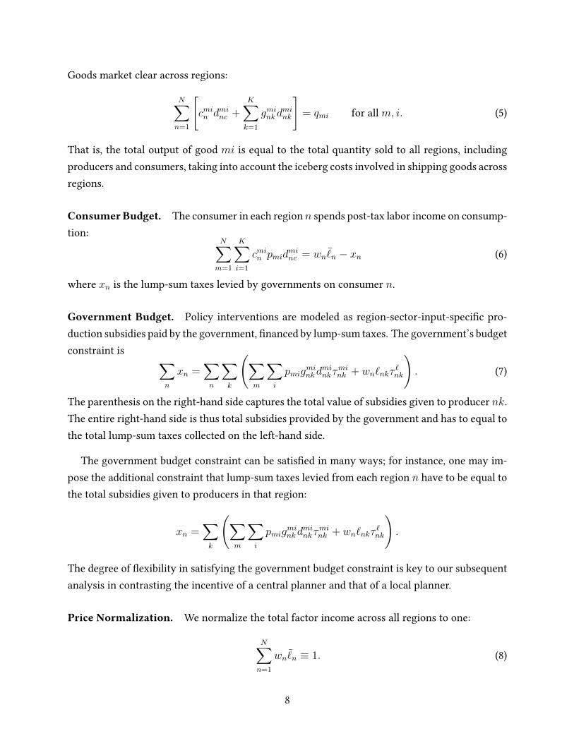
Goods market clear across regions:

N∑n=1

[cmin d

minc +

K∑k=1

gminkdmink

]= qmi for all m, i. (5)

That is, the total output of good mi is equal to the total quantity sold to all regions, includingproducers and consumers, taking into account the iceberg costs involved in shipping goods acrossregions.

Consumer Budget. The consumer in each region n spends post-tax labor income on consump-tion:

N∑m=1

K∑i=1

cmin pmidminc = wn ¯

n − xn (6)

where xn is the lump-sum taxes levied by governments on consumer n.

Government Budget. Policy interventions are modeled as region-sector-input-specic pro-duction subsidies paid by the government, nanced by lump-sum taxes. The government’s budgetconstraint is ∑

n

xn =∑n

∑k

(∑m

∑i

pmigminkd

minkτ

mink + wn`nkτ

`nk

). (7)

The parenthesis on the right-hand side captures the total value of subsidies given to producer nk.The entire right-hand side is thus total subsidies provided by the government and has to equal tothe total lump-sum taxes collected on the left-hand side.

The government budget constraint can be satised in many ways; for instance, one may im-pose the additional constraint that lump-sum taxes levied from each region n have to be equal tothe total subsidies given to producers in that region:

xn =∑k

(∑m

∑i

pmigminkd

minkτ

mink + wn`nkτ

`nk

).

The degree of exibility in satisfying the government budget constraint is key to our subsequentanalysis in contrasting the incentive of a central planner and that of a local planner.

Price Normalization. We normalize the total factor income across all regions to one:

N∑n=1

wn ¯n ≡ 1. (8)

8

2.2 Equilibrium

Denition 1. Equilibrium. Given productivities znk, iceberg trade costs dmink and dminc , mar-ket imperfections χmink , industrial policies

τmink , τ

`nk

, an equilibrium is the collection of prices

pnk, wn, allocations qnk, `nk, gmink , cmin , lump-sum taxes xn, such that: a) the consumer in eachregion chooses consumption to maximize utility (1) subject to budget constraint (6); b) producerschoose allocations to solve cost-minimization problems (3), setting prices to production costs;c) given inputs, production outputs satisfy the production functions (2); d) markets for the fac-tor and intermediate goods clear according to (4) and (5); e) government budget constraint (7) issatised; f) total labor income across all regions sums to one according to the normalization (8).

Denition 2. A Market Equilibrium is an equilibrium in which there are no subsidies or lump-sum taxes: τmink = τ `nk = xn = 0 for all n, k,m, i.

Absent market imperfections or industrial policies, our model coincides with the internationaltrade model of Caliendo and Parro (2015) without taris. The rst welfare theorem holds despitethe presence of iceberg trade costs, and the economy is Pareto ecient.

In the presence of market imperfections (χmink > 0 for some n, k,m, i), the market equilibriumis Pareto inecient, and, as we show, industrial policies may improve welfare for consumers inall regions.

Our theoretical results derive sucient statistics for the rst-order changes in regional welfareun in response to industrial policies introduced to the market economy. Because of inter-regionaltrade, industrial policy targeting any region-industry may have general equilibrium eects andaect consumer welfare in all other regions. The impact of industrial policy also depends on howit is nanced, i.e., who is being taxed.

We later apply these sucient statistics to empirical study industrial policies in China. Acentral theme of our empirical application is to contrast 1) the incentives of a hypothetical centralplanner who wants to improve consumer welfare in all regions and has the ability to collect taxesfrom all regions, and 2) the incentives of a hypothetical regional planner who wants to improvethe welfare of consumers in a specic region and has the ability to levy lump-sum tax only fromthat region.

2.3 Notations

We use the following notations throughout the paper. We use bold math font to denote vectors(lowercase letters) and matrices (uppercase letters).

9

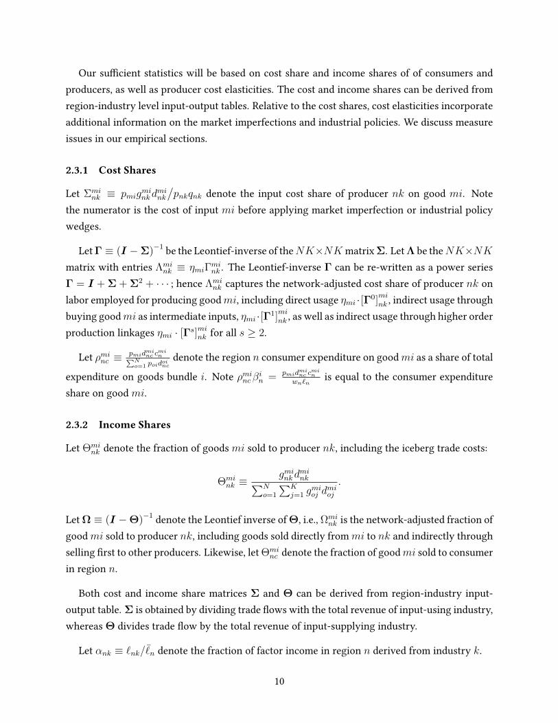
Our sucient statistics will be based on cost share and income shares of of consumers andproducers, as well as producer cost elasticities. The cost and income shares can be derived fromregion-industry level input-output tables. Relative to the cost shares, cost elasticities incorporateadditional information on the market imperfections and industrial policies. We discuss measureissues in our empirical sections.

2.3.1 Cost Shares

Let Σmink ≡ pmig

minkd

mink

/pnkqnk denote the input cost share of producer nk on good mi. Note

the numerator is the cost of input mi before applying market imperfection or industrial policywedges.

Let Γ ≡ (I −Σ)−1 be the Leontief-inverse of theNK×NK matrix Σ. Let Λ be theNK×NKmatrix with entries Λmi

nk ≡ ηmiΓmink . The Leontief-inverse Γ can be re-written as a power series

Γ = I + Σ + Σ2 + · · · ; hence Λmink captures the network-adjusted cost share of producer nk on

labor employed for producing goodmi, including direct usage ηmi · [Γ0]mink , indirect usage through

buying goodmi as intermediate inputs, ηmi ·[Γ1]mink , as well as indirect usage through higher order

production linkages ηmi · [Γs]mink for all s ≥ 2.

Let ρminc ≡pmid

minc c

min∑N

o=1 poidoinc

denote the region n consumer expenditure on goodmi as a share of total

expenditure on goods bundle i. Note ρminc βin = pmidminc c

min

wn`nis equal to the consumer expenditure

share on good mi.

2.3.2 Income Shares

Let Θmink denote the fraction of goods mi sold to producer nk, including the iceberg trade costs:

Θmink ≡

gminkdmink∑N

o=1

∑Kj=1 g

mioj d

mioj

.

Let Ω ≡ (I −Θ)−1 denote the Leontief inverse of Θ, i.e., Ωmink is the network-adjusted fraction of

goodmi sold to producer nk, including goods sold directly frommi to nk and indirectly throughselling rst to other producers. Likewise, let Θmi

nc denote the fraction of goodmi sold to consumerin region n.

Both cost and income share matrices Σ and Θ can be derived from region-industry input-output table. Σ is obtained by dividing trade ows with the total revenue of input-using industry,whereas Θ divides trade ow by the total revenue of input-supplying industry.

Let αnk ≡ `nk/¯n denote the fraction of factor income in region n derived from industry k.

10

Let Tmn ≡∑K

k=1 αmk∑N

o=1 Ωmkoi Θoi

nc be the fraction of factor income in regionm that is derived,directly and indirectly through input-output linkages, from selling to the consumer in region n.

2.3.3 Cost Elasticity

Let Σmink denote the cost elasticity of good nk with respect to input mi. In a market equilibrium,

Σmink = Σmi

nk (1 + χmink), and in matrix form Σ = Σ χ. That is, market imperfection (1 + χmink)

is equal to the ratio between cost elasticity and the cost share in a market equilibrium. Withindustrial policies, Σmi

nk = Σmink (1 + χmink) (1− τmink ).

Let Γ ≡(I − Σ

)−1

denote the Leontief-inverse of Σ; its entry Γmink captures the cost elasticityof good nk with respect to the productivity zmi of good mi, holding constant all factor prices wn.Intuitively, TFP shock for good mi aects the cost of good nk through the direct use of inputmi in the production of good nk, as well as indirect use through higher rounds of input-outputlinkages; the Leontief-inverse captures all higher round eects.

We analogously dene Λmink ≡ ηmiΓ

mink ; this is the elasticity of output nk with respect to labor

hired in mi, holding all inputs costs.

We let ρmink ≡ Σmink

/σink denote the cost elasticity of good nk with respect to input mi relative

to the cost elasticity with respect to the every input in bundle i. Note∑N

m=1 Σmink = σink, hence∑

m ρmink = 1.

2.3.4 Additional Notations

Let γnk denote the total revenue of industry k in region n. Let Arj,qsmi ≡ θ(∑

o ρojniΛ

qsoj − Λqs

rj

); as

we show below, Arj,qsmi is the cross-price elasticity of expenditure by producermi on good rj withrespect to subsidies to labor inputs for good qs. Likewise, dene Arj,qsmc ≡ θ

(∑o ρ

ojncΛ

qsoj − Λqs

rj

),

which is the cross-price elasticity of expenditure by consumer m on good rj with respect tosubsidies to labor inputs for good qs.

2.4 First-Order Sucient Statistics for Evaluating Industrial Policy

In this section we derive sucient statistics for the distributional and aggregate impact of indus-trial policy. We begin by analyzing on subsidies τ `mi to value-added inputs, and we later showthe same welfare sucient statistics hold for subsidies to intermediate inputs as well. We pro-ceed in three steps. First, in Proposition 1 we derive the rst-order general equilibrium responseof regional factor income d lnwn to a set of region-industry subsidies

dτ `mi

and regional

lump-sum taxes dxn, starting from a market equilibrium. Second, in Proposition 2 we derive

11

the general equilibrium response of welfare d lnun in every region to subsidies and lump-sumtaxes. Third, we use Proposition 2 to derive the distributional welfare impact of value-added sub-sidies by requiring the government budget to balance. We derive welfare sucient statistics forlocal industrial policies, i.e., subsidies applied to industries in a specic region and nanced bylump-sum taxes levied from the same region. We also posit a social welfare function to aggregateregional welfare, and we derive sucient statistics for central industrial policies where subsidiesare nanced by lump-sum taxes that is distribution-neutral under our social welfare function.

Proposition 1. Factor Income Response to Industrial Policies. To rst-order, introducingregion-industry factor subsidies

dτ `mi

and regional lump-sum taxes dxn to the market equilib-

rium generates factor price response d lnwn that solves

d lnwn︸ ︷︷ ︸income eect

=∑k

αnk dτ `nk︸ ︷︷ ︸subsidies

+∑m

T nm

(d lnwm −

dxmwm ¯

m

)︸ ︷︷ ︸

market size eect

+θN∑

o,m,q=1

K∑k,j,s=1

αnkΩnkoj

(ΘojmcA

oj,qsmc +

K∑i=1

ΘojmiA

oj,qsmi

)(d lnwq − dτ `qs

)︸ ︷︷ ︸

cross-substitution eect

.

Proof. We begin by re-writing goods market clearing condition as

γnk =∑m

(wm`m − xm) βkmρnkmc +

∑mi

γmiΣnkmi.

Totally-dierentiating,

dγnk =∑m

(wm`m − xm) βkm dρnkmc +∑m

(`m dwm − dxm) βkmρnkmc +

∑mi

γmi dΣnkmi + Σnk

mi dγmi.

Dividing both sides by γnk and recognizing that in a market τ `mi = xm = 0 in a market equilib-rium,

d ln γnk =∑m

Θnkmc

(d ln ρnkmc + d lnwm −

dxmwm`m

)+∑mi

Θnkmi

(d ln Σnk

mi + d ln γmi).

Moving Σnkmi d ln γmi to the left-hand side and recognizing Ω ≡ (I −Θ)−1, we obtain

d ln γnk =∑oj

Ωnkoj

(∑m

Θojmc

(d ln ρojmc + d lnwm −

dxmwm`m

)+∑mi

Θojmi d ln Σoj

mi

). (9)

12

Now recognizewn`n =

∑k

ηnkγnk1− τ `nk

.

Totally dierentiate and again recognize τ `nk = 0 in a market equilibrium,

d lnwn =∑k

αnk(

d ln γnk + dτ `nk).

Substitute out d ln γnk using (9):

d lnwn−∑k

αnk dτ `nk =∑k

αnk∑oj

Ωnkoj

(∑m

Θojmc

(d ln ρojmc + d lnwm −

dxmwm`m

)+∑mi

Θojmi d ln Σoj

mi

).

(10)The last step is to solve for d ln ρojmc and d ln Σoj

mi as a functions of industrial policies and changesin factor prices. Given CES demand,

d ln ρojmc = θ

(∑r

ρrjmc d ln prj − d ln poj

)=

∑rs

Arj,qsmc ( d lnwq − dτqs) .

Likewise,d ln Σoj

mi =∑rs

Arj,qsmi ( d lnwq − dτqs) .

Substitute into (10) and using the denition of T nm,

d lnwn −∑k

αnk dτ `nk −∑m

T nm

(d lnwm −

dxmwm`m

)

=N∑

o,m,q=1

K∑k,j,s=1

αnkΩnkoj

(ΘojmcA

oj,qsmc +

K∑i=1

ΘojmiA

oj,qsmi

)(d lnwq − dτ `qs

),

as desired.

Proposition 1 enables one to solve, to rst-order, the general equilibrium changes in factorincome when introducing factor subsidies and lump-sum taxes into the market equilibrium.

Intuitively, the general equilibrium change in factor income d lnwn can be decomposed intothree eects. First, factor income is increasing in the proportional factor subsidies given to theproducers in the region, with the overall eect

∑k αnk dτ `nk being the average subsidies across

industries weighted by the share of factor income earned from each industry k.

13

Second, factor income in region n depends on the disposable income of consumers from allother regionsm. When consumerm has more income to spend—either because of higher incomed lnwm or lower lump-sum taxes dxm/ (wm`m)—the spending raises the demand for goods that,directly or indirectly, uses the factor in regionn for production. The extent to which factor incomein n increases depends on the fraction n’s income that is derived, directly and indirectly throughthe input-output linkages, from selling to the consumer in region m. We call this the market sizeeect.

Third is the substitution eect. The term d lnwq − dτ `qs captures the increase in the eec-tive cost of factor inputs for good qs; it raises the unit cost of not only good qs but also anyother good that indirectly uses good qs as production inputs. As varieties of good bundle j be-come more expensive, consumers and producers in all regions m and industries i will substitutetowards goods oj and away from varieties of good bundle j produced in other regions. The ex-tent of cross-substitution is captured by the cross-price elasticities, Aoj,qsmc and Aoj,qsmi . Finally, thecross-substitution eect passes down to the factor income in n because good oj may directly orindirectly use factor n in production, hence the terms αnkΩnk

oj Θojmc and αnkΩnk

oj Θojmi. These terms

are the network-adjusted share of factor income in n derived from selling to consumer m andproducer mi, respectively; these terms therefore capture the fraction of n’s factor income that issubject to the substitution eect that takes place in m.

Proposition 2. Welfare Response to Industrial Policies. To rst-order, introducing region-industry factor subsidies

dτ `mi

and regional lump-sum taxes dxn to the market equilibrium

generates regional welfare response d lnun that solves

d lnun = d lnwn −dxnwn ¯

n︸ ︷︷ ︸change in income

−N∑

m,q=1

K∑i,s=1

βinρminc Λqs

mi

(d lnwq − dτ `qs

)︸ ︷︷ ︸

cost-of-living eect

.

Proof. The change in welfare of consumer n is dierence between the log-change in n’s dispos-able income, d lnwn − dxn

wn ¯n

, and the log-change in the consumer price index of region n. Thelatter can be written as the expenditure share-weighted average of price changes of goods mi,∑

m

∑i β

inρ

minc d ln pmi. The proof is complete by recognizing that

d ln pmi =∑q

∑s

Λqsmi

(d lnwq − dτ `qs

).

Denition 3. We dene the local intervention index ζLnk of sector k in region n to be the elasticity

14

of welfare in region n to subsidy spending to good nk, i.e.,

ζLnk ≡d lnunαnk dτ `nk

,

when the lump-sum taxes are levied from consumer n such that government budget is balancedwithin each region: xn =

∑k

(τ `nkwn`nk

). We refer to industrial policies with locally balanced

budget as locally nanced industrial policies.

The local intervention index of industry k in region n local welfare response when local in-dustrial policy is nanced by local taxes. Starting from a market equilibrium, a benevolent localplanner in region n should subsidize sectors with higher ζLnk.

We use the Bergson-Samuelson social welfare function for a central planner:

lnuC =∑n

wn ¯n lnun.

By using the regional factor income as the Pareto weight, the central planner has no incentive toredistribute across regions at the initial equilibrium.

Denition 4. We dene the central intervention index ζCnk of sector k in region n to be the elas-ticity of social welfare uC to subsidy spending τ `nk to the market equilibrium, i.e.,

ζCnk ≡d lnuC

wn`nk dτ `nk

, when the lump-sum taxes are levied from all regions in proportion to the initial regional income:

xm =wm ¯

m∑wm ¯

m

×∑n

∑k

(τ `nkwn`nk

)for all m.

We refer to industrial policies nanced with these taxes as centrally nanced industrial policies.

The local intervention index captures the “bang-for-the-buck” of industrial policy subsidiesdirected towards specic industries when viewed from the perspective of each region. The centralintervention index captures the bang-for-the-buck of industrial policy targeted region-industrysubsidies evaluated using the Bergson-Samuelson social welfare function.

The next several Propositions show how the intervention indices are sucient statistics forevaluating industrial policies.

Proposition 3. The local intervention index averages to zero across industries when weighted by

15

industry-level employment shares:

K∑k=1

αnkζLnk = 0 for all n.

The central intervention index average to zero across industries and regions when weighted by factorincome share

N∑n=1

K∑k=1

wn`nkζCnk = 0.

Proposition 4. Let SpendingLnk denote the total scal cost of locally nanced subsidies directed tothe production of good nk:

SpendingLnk ≡ αnkτ`nk.

Then to rst order, relative to the market economy,

∆un =∑k

ζLnk × SpendingLnk. (11)

If instead the subsidies are centrally nanced, let SpendingCnk denote the total scal cost of centrallynanced subsidies directed to the production of good nk:

SpendingCnk ≡ wn`nkτ`nk.

Then to rst-order, relative to the market economy

∆uC =∑n

∑k

ζCnk × SpendingCnk. (12)

Corollary 1. Equations (11) and (12) can be re-written as the covariance between the respectiveintervention index and the subsidy spendings per sectoral value-added:

∆un = CovL(ζLnk,

SpendingLnk`nk/¯

n

),

∆uC = CovC(ζCnk,

SpendingCnkwn`nk

),

16

where CovL is the covariance operator taken across industries, using the local income share fromeach industry as the distribution;1 CovC is the covariance operator taken across region-industries,using each region-industry’s value-added as the distribution.2

Relation to the Literature. In a single-region economy, the local and central interventionindices coincide and are both equal to the distortion centrality (minus a constant) proposed byLiu (2019).

Industrial policies aect factor income because subsidies change prices and lump-sum taxeschange disposable income. The price impact of subsidies is analogous to that of productivityshocks; in fact, the factor income response to TFP shock is

d lnwn =∑k

αnk dτ `nk +∑m

T nm ( d lnwm)

+N∑

o,m,q=1

K∑k,j,s=1

αnkΩnkoj

(ΘojmcA

oj,qsmc +

K∑i=1

ΘojmiA

oj,qsmi

)(d lnwq −

d ln zqsηqs

),

which is the result of Kleinman et al. (2020).

If consumers across all regions face the same iceberg trade costs for each good (dminc = dmioc forall n, o,m, i), then there exists a representative consumer for the multi-region economy. Supposefurther that industrial policy takes the form of a single subsidies τqs to each producer that appliesequally to all inputs: dτqs ≡ dτ `qs = dτ ojqs for all q, s, o, j. Then

1CovL (ank, bnk) =∑

k`nk¯nankbnk −

(∑k

`nk¯nank

)(∑k

`nk¯nbnk

).

2CovC (ank, bnk) =∑

n

∑k wn`nkankbnk − (

∑n

∑k wn`nkank) (

∑n

∑k wn`nkbnk).

17

d lnuC = −∑n

∑k

γnk dτnk −∑n

wn`n

N∑m,q=1

K∑i,s=1

βinρminc Λqs

mi

(d lnwq −

dτqsηqs

)

=∑n

wn`n

N∑m,q=1

K∑i,s=1

βinρminc

Λqsmi

ηqsdτqs

−

(∑n

∑k

γnk dτnk +∑n

wn`n

N∑m,q=1

K∑i,s=1

βinρminc Λqs

mi d lnwq

)

=∑n

wn`n

N∑m,q=1

K∑i,s=1

βinρminc

Λqsmi

ηqsdτqs

−

(∑n

wn`n

N∑m,q=1

K∑i=1

βinρminc

K∑s=1

Λqsmi d ln

wq1−

∑n

∑k γnk dτnk

).

This is analogous to Baqaee and Farhi (2020) Theorem 1, which concerns the aggregate impactof markups. The term

∑n,m,iwn`nβ

inρ

minc Λqs

mi/ηqs corresponds to the cost-based Domar weight ofsector qs,

∑n,m,i,s β

inρ

minc Λqs

mi is the cost-based Domar weight of factor q, and d lnwq1−

∑n

∑k γnk dτnk

isthe log-change in the revenue based the Domar weight of factor q.

3 Empirical Results

3.1 Intervention Index

We use the 2012 multi-regional input-output table of China, the most recent version released byChina’s National Bureau of Statistics (henceforth NBS). The input-output table covers a total of 42industries and all the 31 provinces. The detailed description of industry classication is providedin Appendix A. We obtain 1273 region-industry pairs after excluding those associated with zerosales in the input-output table.

Liu (2019) has shown that central intervention indices are very robust to wedges. We rstassume a constant wedge of 10% for each region-industry pair. The corresponding central andlocal intervention indices are used as our benchmark measures.3 We next simulate central andlocal intervention indices by randomly drawing region-industry-specic wedges from dierentdistributions assumed in Liu (2019). Table 1 shows that the simulated intervention indices arehighly correlated with the benchmark, suggesting that both central and local intervention indicesbe primarily determined by the structure of production network, rather than wedges. We will use

3Data source see Liu et al. (2018).

18

intervention indices with constant wedge in the following analysis. However, all the results arerobust to randomly simulated wedges.

Table 1: Average Correlation with Benchmark across Dierent Specications

Pearson’s r Spearman’s ρ

Specications Central Local Central Local

constant χij = 5% 1.00 0.97 1.00 0.95log ∼ N(0.09, 0.1) 0.93 0.98 0.95 0.97N(0.1, 0.1) 0.95 0.98 0.96 0.98N(0.2, 0.2) 0.91 0.93 0.93 0.92maxN(0.1, 0.1), 0 0.97 0.99 0.98 0.99U [0, 0.1] 0.98 0.97 0.99 0.95U [0, 0.2] 0.98 0.99 0.99 0.99Exp(0.1) 0.96 0.99 0.97 0.98Exp(0.15) 0.96 0.97 0.97 0.97

Notes: We simulate intervention indices for 100 times under each distributional assumption. This table reports theaverage correlation coecient between the benchmark and simulated intervention indices under each distributionalassumption.

The summary statistics of the intervention indices are reported in Table 2. The average of localintervention index is close to that of central intervention index. However, local intervention in-dex has a substantially larger variation. The maximum and minimum value of local interventionindex is 0.95 and -0.40, respectively, about a third higher and a quarter lower than its counter-part of central intervention index. The more dispersed local intervention index suggests highersensitivity of local welfare to industrial policy.

Table 2: Summary Statistics

N Mean Median Max Min Std

ζC 1273 0.01 -0.01 0.41 -0.22 0.12ζL 1273 0.05 0.03 0.95 -0.40 0.16

Moreover, the correlation between central and local intervention index is low. The correlationcoecient weighted by value added is only 0.24. There are two main reasons for the low corre-lation. First, central intervention index of an industry is mainly determined by its upstreamness,which is similar across regions. Therefore, industry xed eects account for 90% of the variationsin central intervention index (see Column 2 in Table 3).

The determination of local intervention index is more involved. Industry xed eects onlyaccount for 23% of the variations in local intervention index. The regional trade linkages play an

19

Table 3: Region and Industry Eect

Central Intervention Index Local Intervention Index

(1) (2) (3) (4) (5) (6)

R-squared 0.00406 0.902 0.934 0.00147 0.225 0.228

Province Dummy YES NO YES YES NO YESIndustry Dummy NO YES YES NO YES YESN 1273 1273 1273 1273 1273 1273Standard errors in parentheses∗ p < 0.1, ∗∗ p < 0.05, ∗∗∗ p < 0.01

important role. Table 4 reports the summary statistics of several model-free indicators for China’sprovince-to-province production and trade network. Table 5 shows that the correlations betweenintervention index measures and the indicators.4 Central and local intervention index are generi-cally dierent in their correlations with “non-local intermediate share”, – i.e., the proportion of aregion-industry output used as intermediate input outside the region. The correlation is positivefor central intervention index but negative for local intervention index. Intermediate goods soldto the other regions do not directly benet the local economy and are therefore discounted in lo-cal intervention index. In contrast, central intervention index internalizes the positive spilloversof local production to the other regions.

In summary, despite the similarity of the vertical structure of production network across re-gions, the dierences between central and local intervention index are substantial. In the follow-ing empirical analysis, we will use the dierences to shed lights on central and local industrialpolicies.

4The results for index_central_nonlocal are shown in Table A.3 in Appendix A.

20

Table 4: Summary of Statistics

N Mean Median Max Min Std

share of sales as nal use 1273 0.37 0.32 1.00 0.00 0.32share of sales as local input 1273 0.52 0.53 1.00 0.00 0.28share of sales as non-local input 1273 0.12 0.06 0.93 0.00 0.15index_local 1273 1.00 1.00 1.50 0.58 0.07index_central 1273 1.00 1.00 2.18 0.74 0.08index_central_nonlocal 1273 1.00 1.00 1.22 0.00 0.09

Notes: We use the 2012 multi-regional input-output table of China. All the indicators are calculated at the region-industry level. For industry k in region n, ζLnk and ζCnk denote local intervention index and central interventionindex, respectively. We decompose nk’s total output into three parts: intermediate input used locally; intermedi-ate input used by other regions and nal use. share of sales as nal use is calculated as

∑m Θnk

mf , the sales shareof nal use; share of sales as local input equals to

∑i Θnk

ni , which is the share of sales used as intermediate inputsin local production; share of sales as non-local input is calculated as 1 −

∑m Θnk

mf −∑

i Θnkni , which is the share

of sales used as intermediate inputs by production outside the region; index_local denotes the average local inter-vention index of all the local users in the region-industry pair nk,

∑i(sales

nkni /

∑i sales

nkni )ζLni, where salesnkni is

ni’s expenditure on nk; index_central denotes the average central intervention index of all the local users in nk,∑i(sales

nkni /

∑i sales

nkni )ζCni; and index_central_nonlocal denotes the average central intervention index of all the

users outside region n,∑

m6=n

∑j(sales

nkmj/

∑m 6=n

∑j sales

nkmj)ζ

Cmj .

21

Table 5: Intervention Index

Panel A: Central Intervention Index

(1) (2) (3) (4) (5) (6)

share of sales as local input 0.303∗∗∗ 0.134∗∗∗ 0.282∗∗∗ 0.264∗∗∗ 0.207∗∗∗ 0.227∗∗∗(0.00863) (0.0122) (0.00776) (0.0130) (0.00599) (0.0108)

share of sales as non-local input 0.397∗∗∗ 0.235∗∗∗ 0.249∗∗∗ 0.199∗∗∗(0.0235) (0.0168) (0.0128) (0.0122)

index_central 0.832∗∗∗ 0.469∗∗∗(0.0353) (0.0411)

R-squared 0.610 0.953 0.820 0.967 0.935 0.981

Panel B: Local Intervention Index

(1) (2) (3) (4) (5) (6)

share of sales as local input 0.208∗∗∗ 0.535∗∗∗ 0.233∗∗∗ 0.0161 0.202∗∗∗ 0.127∗∗∗(0.0114) (0.0399) (0.0100) (0.0431) (0.00821) (0.0351)

share of sales as non-local input -0.457∗∗∗ -0.936∗∗∗ -0.344∗∗∗ -0.654∗∗∗(0.0345) (0.0598) (0.0214) (0.0440)

index_local 1.024∗∗∗ 0.904∗∗∗(0.0492) (0.0539)

R-squared 0.236 0.469 0.464 0.649 0.692 0.774

Province Dummy YES YES YES YES YES YESIndustry Dummy NO YES NO YES NO YESN 1273 1273 1273 1273 1273 1273Standard errors in parentheses∗ p < 0.1, ∗∗ p < 0.05, ∗∗∗ p < 0.01

Notes: Dependent variables in Panel A are central intervention indices; and dependent variables in Panel B are localintervention indices.

22

3.2 Policy Platforms

The distinctive dierences between central and local intervention index imply testable predic-tions for central and local industrial policies. Liu (2019) provides evidence for policies in favorof the industries with high central intervention index, which can be interpreted as central indus-trial policy through the lens of our model. In the countries with empowered local governments,there should be room for local industrial policies that aim to improve local welfare rather thanaggregate welfare.

China has a particularly strong local state capacity (Bai et al., 2020a). Local governments oftenfavor local rms and industries by bending policies and regulations set by the central government(Bai et al., 2020b). Moreover, local governments have discretions in allocating self-raised fundfrom selling local land use rights and borrowing through local nancing vehicles (Bai et al., 2016;Song and Xiong, 2018). While personnel decisions on high-ranked ocials are made by the centralgovernment, the promotion likelihood of local ocials is related to local economic performancein their tenure (e.g., Li and Zhou, 2005). Local ocials also benet directly from local economicdevelopment.5 In short, Chinese local ocials are endowed with substantial resources and well-motivated to promote local industrial policies.

The empirical challenge is that many industrial policies are not observable. Distinguishingcentral and local industrial policies is even harder. Instead of directly identifying industrial poli-cies, we infer them indirectly from central and local “policy platforms”. One example is Spe-cial Economic Zone (SEZ), is perhaps the most popular platform for industrial policy around theworld. Like many other countries, China has used SEZs to support targeted industries. As of 2018,China established 2543 SEZs. Industrial upgrading is one of SEZ’s missions. Each SEZ speciesabout 3 priority industries. A key to our analysis is that a quarter of SEZs were approved by thecentral government and the rest were approved by provincial governments. We can infer centraland local industrial policies from the industries prioritized by central and local SEZs, respectively.

Another policy platform is the state sector. Bai et al. (2020b) show that the state sector ac-counted for about a quarter of capital in China in 2019. It has been widely documented that manystate-owned enterprises (SOEs) are supported by discriminative policies and subsidies (Hsieh andSong, 2015; König et al., 2020). Many of the policies and subsidies target SOEs in specic indus-tries. For example, the central government explicitly identied 7 strategic industries and 9 pillarindustries to be controlled and dominated by the state sector, respectively (Document No. 97,General Oce of the State Council, 2006). The share of SOEs in an industry is thus a mani-

5See Xu (2011) and Bai et al. (2020a) for local ocials’ incentives of promoting local economy in additional to thepromotion incentives.

23

festation of the intensity of industrial policy on the platform. Analogous to SEZs approved bycentral and local government, in our sample, 40% of SOEs are directly controlled by the centralgovernment and central SOEs account for 65% of total capital owned by the state. The rest ofSOEs are controlled by various levels of local governments. We can therefore infer central andlocal industrial policies from variations in the share of central and local SOEs across regions andindustries.

If the central government exerts full control over local governments, central industrial policiescan also be implemented through local policy platforms. However, the standard principle-agentproblem would arise whenever the control is imperfect. The resources for central industrial poli-cies can be diverted by local SEZs or SOEs for other purposes. Therefore, the central governmentis be more willing to implement central industrial policies through the units controlled by them-selves. This leads to the following hypotheses that can be tested by the data.

1. The intensity of central (local) industrial policy should be stronger in the industries withhigher central (local) intervention index.

2. The correlation between the intensity of local industrial policy and local intervention indexshould be stronger for the policies associated with more divertible resources and in theregions where the central government exerts less control over the local government.

3.2.1 Special Economic Zone

We extract information from Catalogue of China’s Development Zones (2018 version) to constructour SEZ measures. Among the 2543 SEZs approved up to 2018, 552 and 1991 SEZs were approvedby central and provincial governments, respectively. We code the industries targeted by eachSEZ according to the industry classications in our input-output table. We then construct twoprovince-industry-specic measures for the intensity of industrial policy on the SEZ platform: thelikelihood for the industry to be targeted by central and local SEZs in the province, respectively,referred to as central and local SEZ intensity.

The correlations between SEZ intensities and intervention indices are reported in Table 6. Thelikelihood of an industry to be targeted by both central and local SEZs is positively correlatedwith central intervention index but uncorrelated with local intervention index. We interpret thecorrelations as evidence for central industrial policies implemented through SEZs. Local SEZintensity turns out to be more correlated with central intervention index than local interventionindex. The weaker correlation with local intervention index does not necessarily disapprovelocal industrial policies. Rather, it seems in line with the second hypothesis for the following tworeasons. First, the central government can easily monitor the priority industries selected by local

24

government. Moreover, the central government seldom provides subsidy for local SEZs. Bothalleviate the principle-agent problem for local SEZs to implement central industrial policies.

Table 6: Special Economic Zone: Central v.s. Local

log(central SEZ intensity) log(local SEZ intensity)

(1) (2) (3) (4) (5) (6)

central intervention index 2.037∗ 2.241∗ 2.918∗∗∗ 3.498∗∗∗(1.159) (1.170) (0.836) (0.839)

local intervention index 0.0939 -0.454 -0.397 -1.248∗∗(0.618) (0.549) (0.530) (0.508)

Province Dummy YES YES YES YES YES YESIndustry Dummy NO NO NO NO NO NON 346 346 346 484 484 484R-squared 0.149 0.119 0.152 0.238 0.194 0.252Standard errors in parentheses∗ p < 0.1, ∗∗ p < 0.05, ∗∗∗ p < 0.01

3.2.2 State Share

Our second empirical analysis is to examine if the size of the state sector correlates to centraland local intervention index across industries and regions. The ocial statistics only reveal theshare of SOEs in the industrial sector. We overcome the diculty by using the 2015 rm reg-istration records of China’s State Administration for Market Regulation, which provide owner-ship and registration information for all the 17 million active rms in that year. Following Baiet al. (2020b), we work through the ownership chain to identify each rm’s ultimate owners,who can be government units, private individuals and foreign legal persons. We then calculatethe province-industry-specic central and local state share, dened as the proportion of capi-tal owned by central and local governments in the total capital of the province-industry pair,respectively. Local governments include provincial and lower level governments.

We nd a striking dichotomy between central and local state shares. The rst column in Table 7shows that central state share is highly correlated with central intervention index. Its correlationwith local intervention index is much weaker (Column 2) and disappears entirely when centralintervention index is added to the regression (Column 3). In contrast, local state share is alwayshighly correlated with local intervention index but uncorrelated with central intervention index(Column 4 to 6). These ndings are consistent with the second hypothesis implied by our model.

We also nd dierent correlations between state shares and intervention indices across re-gions. We group the 30 Chinese provinces into three regions: East China, Central China, West &Northeast China. East China has the highest GDP per capita, which is 64% and 83% higher than

25

Table 7: State Share and Intervention Index

log(central state share) log(local state share)

(1) (2) (3) (4) (5) (6)

central intervention index 3.798∗∗∗ 3.659∗∗∗ 0.487 0.125(0.685) (0.690) (0.701) (0.728)

local intervention index 1.317∗ 0.559 1.535∗∗∗ 1.509∗∗∗(0.694) (0.682) (0.545) (0.580)

Province Dummy YES YES YES YES YES YESIndustry Dummy NO NO NO NO NO NON 1118 1118 1118 1209 1209 1209R-squared 0.231 0.188 0.232 0.105 0.120 0.120Standard errors in parentheses∗ p < 0.1, ∗∗ p < 0.05, ∗∗∗ p < 0.01

the GDP per capita of Central China and West & Northeast China, respectively, in 2018. We runthe same regressions for each region and report the results in Table 8. Central state share pos-itively correlates to central intervention index in all the three regions. The positive correlationis robust to adding local intervention index in the regression, except for East China. Local stateshare is uncorrelated with central intervention index in East China and West & Northeast Chinabut positively correlated with central China. Moreover, the positive correlation between localstate share and local intervention index is mainly driven by East China. These ndings suggestthe correlations between state shares and intervention indices are correlated with regional in-come level. In particular, there is evidence for local industrial policy implemented through bothcentral and local SOEs in East China, the most developed region.

To further explore the variations in the correlations, we run the regressions in Column 3 and 6province by province. Panel A and B in Figure 1 plot the estimated coecients of central and localintervention index in the regression for central state share, respectively. In line with the resultsin Table 8, the estimated coecients of central intervention index are positive in 26 out of 30provinces. Only a third of the provinces have a positive estimated coecient of local interventionindex6. None of the two estimates is correlated with provincial income.

Panel C and D plot the estimated coecient of central and local intervention index in theregression for local state share, respectively. Consistent with the results in Table 8, the estimatedcoecient of central intervention index is positive in 19 provinces but turns signicantly negativefor Jiangsu and Zhejiang, the two highest-income provinces in East China. This leads to a negativecorrelation between the estimates and provincial income, which is statistically signicant at the

68 out of 11 positive estimated coecient of local intervention index are insignicant. 2 out of 3 signicantcoecients are in East China.

26

Table 8: State Share and Intervention Index: Regional Results

log(central state share) log(local state share)

(1) (2) (3) (4) (5) (6)

Panel A: East

central intervention index 3.028∗∗∗ 1.793 -0.563 -2.173(1.127) (1.279) (1.215) (1.379)

local intervention index 3.606∗∗∗ 2.889∗∗ 2.941∗∗∗ 3.839∗∗∗(1.185) (1.356) (1.017) (1.249)

N 375 375 375 392 392 392R-squared 0.269 0.285 0.293 0.0398 0.0847 0.105

Panel B: Central

central intervention index 4.068∗∗∗ 4.273∗∗∗ 2.305∗∗ 2.336∗∗(1.268) (1.239) (0.944) (0.917)

local intervention index -0.310 -0.903 0.214 -0.132(0.924) (0.779) (0.692) (0.574)

N 228 228 228 238 238 238R-squared 0.136 0.0738 0.141 0.192 0.158 0.192

Panel C: West & Northeast

central intervention index 4.890∗∗∗ 4.870∗∗∗ 1.054 1.072(0.943) (0.965) (0.906) (0.881)

local intervention index -0.755 -0.625 0.645 0.670(0.863) (0.895) (0.707) (0.721)

N 515 515 515 579 579 579R-squared 0.153 0.0552 0.155 0.141 0.135 0.145

Province Dummy YES YES YES YES YES YESIndustry Dummy NO NO NO NO NO NOStandard errors in parentheses∗ p < 0.1, ∗∗ p < 0.05, ∗∗∗ p < 0.01

Notes: East area covers 10 provinces: 4 provinces (Beijing, Tianjin, Hebei and Shandong) in Circum-Bohai-Sea, 3provinces (Shanghai, Jiangsu and Zhejiang) in Yangtze River Delta, and another 3 provinces (Fujian, Guangdong andHainan) in southeastern costal region; Central area includes 6 provinces: Shanxi, Anhui, Jiangxi, Henan, Hubei andHunan; the remaining 15 provinces are in West & Northeast area.

27

level of 99%. The estimated coecient of local intervention index is positive for 16 provinces,many of which are high-income provinces such as Jiangsu and Zhejiang. The correlation betweenthe estimates and provincial income is positive and statistically signicant at the level of 99%.High-income provinces are more likely to support the industries with high local interventionindex through SOEs. In contrast, low-income provinces are more likely to support the industrieswith high central intervention index.

An interesting question is why industrial policies implemented through SOEs are more in linewith central intervention index in poorer regions? One possibility is that low-income provincesare more dependent of scal transfers from the central government. Local scal revenue onlyaccounted for 42% of local scal expenditure in Central and West & Northeast China, while theratio was 73% for East China and 79% for Jiangsu and Zhejiang7. The correlation coecient be-tween GDP per capita and the ratio of local scal revenue to local scal expenditure is 0.85 acrossprovinces. The scal redistribution alleviates the principle-agent problem between the centraland local governments in implement central industrial policies. Figure 2 shows a strong negativecorrelation between the estimated coecient of central intervention index in the regression forcentral state share and the ratio of of local scal revenue to local scal expenditure. The evi-dence is consistent with the second hypothesis and suggests that the central government be in astronger position to implement central industrial policies in the provinces that are more depen-dent of scal redistribution8.

7Local scal revenue and expenditure data are from website of NBS and data year is 2015.8For robustness check, we trim state share data by top and bottom 5% for each province and re-do all the analysis

in this section. Results are shown in Appendix B and they are quite similar to the full sample results here.

28

Figure 1: State Share Sensitivity to Intervention Index: Provincial Variation

29

Figure 2: Local State Share Sensitivity to Intervention Index: Provincial Variation

30

3.3 Region-Industry-Ownership-Specic Wedges

In this section, we want to understand how the central and local governments implement in-dustrial policies through SOEs. To this end, we use the rm survey data from China’s StateAdministration of Taxation (SAT henceforth). The SAT survey data, which covers both manufac-turing and service industries, has a much better sectoral composition than the Annual Survey ofAbove-Scale Industrial Firms that has been widely used in the literature.

To identify central and local SOEs, we merge the SAT data with the registration data. FollowingHsieh and Song (2015), we take two steps to identify SOEs. First, all the rms registered as SOEsin the SAT data are taken as SOEs. 9 Second, the rms registered as non-SOEs in the SAT databut identied as SOEs by their registration information (i.e., with state share above or equal to50%) are also taken as SOEs. We next dene central and local SOEs in the same way as before.Table 9 reports the summary statistics of rms with three ownership types: private, central andlocal SOEs in our sample. About 5% of the rms are SOEs and 40% of SOEs are central SOEs.

Table 9: Summary Statistics of Sample by Ownership

non-SOE Central SOE Local SOE

Share of Firm Number 95.1% 2.0% 2.9%Share of Sales 80.2% 13.2% 6.6%Share of Capital 64.4% 23.3% 12.3%Share of Labor 83.3% 8.5% 8.2%

Note: For each statistic, we show average number between the year 2011 and 2015; sum of each row is 100%; andaverage annual total rm number is 550931.

We construct three province-industry-ownership-specic wedges: capita, land and labor wedges.Capital wedge is the median value of rm’s sales-to-capital ratio in a province-industry-ownershipgroup between 2011 and 2015. There are 30 provinces, 42 industries consistent with input-outputtable and three ownership types. As a robustness check, we construct year-specic capital wedgeby using the median value of the ratio in each group in each year and control year xed eectin all the regressions below. The results are very robust and reported in Appendix C. FollowingHsieh and Klenow (2009), we interpret the sales-to-capital ratio as the average cost of capital.Lower capital wedge implies lower capital tax or higher capital subsidy.

Similar to capital wedge, we also construct land wedge as the sales-to-land ratio and labor9We use the code for registration type of taxpayer in the SAT data. Taxpayers registered as “state-owned enter-

prise”, “joint-stock cooperative enterprise restructured from state-owned enterprise”, “state-owned associated enter-prise” and “wholly state-owned enterprise” are identied as SOEs.

31

wedge as the sales-to-employment ratio for each region-industry-ownership group. The robust-ness checks are reported in Appendix E.2 and D.2, respectively.

3.3.1 Capital Wedge

Table 10 reports the regression results for capital wedge. In the rst column, we regress capitalproductivity on the dummies for central SOEs and private rms, using local SOEs as the bench-mark group. We add central intervention index and the interactions with ownership dummies.Industry and province xed eects are controlled. Consistent with what has been widely docu-mented in the literature (e.g., Song et al., 2011; Hsieh and Song, 2015), we nd capital productivityof private rms to be signicantly higher than that of SOEs. What is new here is that capital pro-ductivity of central SOEs is higher than that of local SOEs. As we will elaborate in the nextsubsection, the dierence is likely to be explained by stronger market power granted to centralSOEs.

Table 10: Capital Wedge and Intervention Index

(1) (2) (3)

soe_central 0.310∗∗∗ 0.300∗∗∗ 0.315∗∗∗(0.0631) (0.0639) (0.0622)

private 0.683∗∗∗ 0.688∗∗∗ 0.691∗∗∗(0.0505) (0.0497) (0.0495)

central intervention index -0.218 0.0288(0.491) (0.498)

soe_central×central intervention index 0.211 0.0189(0.722) (0.749)

private×central intervention index 1.171∗∗∗ 0.938∗∗(0.412) (0.421)

local intervention index -1.183∗∗∗ -1.066∗∗∗(0.310) (0.323)

soe_central×local intervention index 0.839∗∗ 0.855∗(0.424) (0.451)

private×local intervention index 1.124∗∗∗ 0.992∗∗∗(0.317) (0.331)

Province Dummy YES YES YESIndustry Dummy YES YES YESN 3299 3299 3299R-squared 0.944 0.944 0.944Standard errors in parentheses∗ p < 0.1, ∗∗ p < 0.05, ∗∗∗ p < 0.01

Notes: Dependent variable is log of sales-capital ratio at region-industry-ownership level which is the median valueamong all the rms in each region-industry-ownership group between the year 2011 and 2015; reference group islocal SOEs whose central state share is lower than local state share; dummy variable soe_central equals 1 if it is theregion-industry level sales-capital ratio for SOEs whose central state share is larger than or equal to local state share,otherwise it is 0; dummy variable private equals 1 if it is the region-industry level sales-captial ratio for private rms,otherwise it is 0.

32

Central intervention index is not signicantly correlated with capital productivity among localSOEs. The interaction term with central SOE dummy is also statistically insignicant. In words,there is no evidence for subsidizing capital cost of SOEs as central industrial policy. Note that thisdoes not necessarily contradict the previous ndings. The larger shares of central SOEs in theindustries with higher central intervention index can be driven by other industrial policies suchas entry barriers and discriminative regulations. The interaction between central interventionindex and private rm dummy is positive and signicant. This is a strong rejection of centralindustrial policy implemented by subsidizing capital cost of private rms.

We then replace central intervention index with local intervention index in the regressionsand report the results in the second column of Table 10. The estimated coecients of the own-ership dummies are very robust. The correlation between local intervention index and capitalproductivity is now negative and highly signicant for the benchmark group, indicating that lo-cal SOEs receive more capital subsidies than the average in the industries with local interventionindex above the mean value.10 This provides evidence for local industrial policy implemented bysubsidizing capital cost of local SOEs and is consistent with the larger share of local SOEs in theindustries with higher local intervention index. The interaction between local intervention indexand central SOE or private rm dummy is positive. Adding back the estimate coecient of localintervention index for local SOEs, the estimates of local intervention index are much closer tozero and statistically insignicant.

We include both central and local intervention index and their interactions with ownershipdummies in the third column. The results are similar to those in the rst and second columns.Most importantly, capital productivity remains uncorrelated with central intervention index butnegatively correlated with local intervention index at the signicance level of 1%. the interactionterm between local SOE dummy and local intervention index remains negative, though the levelof signicance is slightly below 5%.

3.3.2 Labor Wedge

Table 11 reports the results for labor wedge. Labor productivity of central SOEs is about a thirdhigher than local SOEs and private rms. Using annual survey of industrial rms, Hsieh andSong (2015) also found higher labor productivity for SOEs after 2007. The labor productivity gapcan be explained by capital intensity if the productivity technology is not Cobb-Douglas. We addcapital-to-labor ratio as a additional control and nd essentially the same results.11 Market poweris another potentially important factor. The average market share of a central SOE in an industry

10Both central and local intervention index have mean values close to one.11The regression results without capital intensity are reported in the Appendix D.1.

33

is 13.2%, twice of a local SOE. This implies that central SOEs be granted with more market powerthan local SOEs, which, in turn, is consistent with higher labor productivity for central SOEs butnot for local SOEs. If we assume that the labor productivity premium for central SOEs is all drivenby markups, the same dierence in markups can also explain nearly all the capital productivitygap between local and central SOEs in Table 10.

The remaining results for labor productivity are similar to those for capital productivity. Theweak correlation between labor productivity and central intervention index does not supportlabor subsidy as central industrial policy implemented through SOEs. Instead, the correlationsbetween labor productivity and local intervention index for local SOEs implies local industrialpolicy by subsidizing local SOEs only.

Table 11: Labor Wedge and Intervention Index: Add Controls

(1) (2) (3)

soe_central 0.353∗∗∗ 0.351∗∗∗ 0.355∗∗∗(0.0551) (0.0553) (0.0546)

private 0.0335 0.0302 0.0344(0.0481) (0.0480) (0.0477)

central intervention index -0.518 -0.306(0.433) (0.423)

soe_central×central intervention index 0.786∗ 0.668(0.420) (0.425)

private×central intervention index 1.089∗∗∗ 0.913∗∗∗(0.340) (0.340)

local intervention index -1.067∗∗∗ -0.945∗∗∗(0.209) (0.213)

soe_central×local intervention index 0.644∗∗ 0.543(0.327) (0.337)

private×local intervention index 0.847∗∗∗ 0.715∗∗∗(0.219) (0.226)

log(capital intensity) 0.336∗∗∗ 0.331∗∗∗ 0.333∗∗∗(0.0361) (0.0366) (0.0364)

Province Dummy YES YES YESIndustry Dummy YES YES YESN 3299 3299 3299R-squared 0.905 0.906 0.907Standard errors in parentheses∗ p < 0.1, ∗∗ p < 0.05, ∗∗∗ p < 0.01

Notes: Dependent variable is log of sales-labor ratio at region-industry-ownership level which is the median valueamong all the rms in each region-industry-ownership group between the year 2011 and 2015; reference group islocal SOEs whose central state share is lower than local state share; dummy variable soe_central equals 1 if it is theregion-industry level sales-capital ratio for SOEs whose central state share is larger than or equal to local state share,otherwise it is 0; dummy variable private equals 1 if it is the region-industry level sales-captial ratio for private rms,otherwise it is 0; log(capital intensity) is the log of capital-labor ratio at region-industry-ownership level which is themedian value among all the rms in each region-industry-ownership group between the year 2011 and 2015.

34

3.3.3 Land Wedge

Industrial land use rights are often sold by local government at a much lower price than residentialland use rights (Bai et al., 2020a). So, it would be interesting to check if industrial policies areimplemented through land subsidy. Dierent from annual survey of industrial rms, the SATdata provides data on land used by each rm. The summary statistics are reported in Table 12.

Table 12: Land Distribution

Private Central SOE Local SOE

Share of Firms with Land Data 36.2% 61.3% 54.1%Land Allocation 62.5% 15.7% 21.8%

Notes: First row shows share of rms that report land usage data for each ownership type. Second row shows landdistribution across ownership types and row sum is 100%.

We run the same regressions as those in Table 11 for land productivity. The results are reportedin Table 13. Like labor productivity, land productivity of central SOEs is higher than local SOEsand private rms. The result is robust to capital intensity. Again, if we assume that the laborproductivity premium is all driven by markups, the same dierence in markups can explain aboutthree quarters of the land productivity gap between central and local SOEs. There is no signicantcorrelation between land productivity and central intervention index for local SOEs and privaterms. The correlation turns positive for central SOEs, indicating that central SOEs pay higherland prices in the industries that should be supported by central industrial policy. All these areagainst land subsidy as central industrial policy. The correlations between land productivity andlocal intervention index are similar to those for capital and labor productivity. Local SOEs areassociated with lower land productivity in the industries with higher local intervention index andthe correlations are much weaker for central SOEs and private rms12.

In summary, we nd (1) no evidence for central industrial policy implemented by capital, laboror land subsidy; (2) evidence consistent with local industrial policy implemented by subsidizinglocal SOEs.

3.3.4 Welfare Analysis

Proposition 4 provides a simple way to assess the magnitude of welfare losses caused by decen-tralized industrial policies. We look at a specic local industrial policy: Subsidizing local SOEsby the correlations between wedges and local intervention index.

12The regression results without capital intensity are reported in the Appendix E.1.

35

Table 13: Land Wedge and Intervention Index: Add Controls

(1) (2) (3)

soe_central 0.433∗∗∗ 0.449∗∗∗ 0.432∗∗∗(0.0761) (0.0766) (0.0762)

private 0.195∗∗∗ 0.202∗∗∗ 0.199∗∗∗(0.0559) (0.0547) (0.0549)

central intervention index 0.849 1.064∗(0.574) (0.581)

soe_central×central intervention index 1.369∗∗ 1.261∗∗(0.578) (0.598)

private×central intervention index 0.723∗ 0.505(0.434) (0.434)

local intervention index -1.156∗∗∗ -1.098∗∗∗(0.351) (0.368)

soe_central×local intervention index 0.712 0.508(0.572) (0.583)

private×local intervention index 0.935∗∗∗ 0.883∗∗(0.357) (0.376)

log(capital intensity) -0.159∗∗∗ -0.155∗∗∗ -0.161∗∗∗(0.0446) (0.0439) (0.0441)

Province Dummy YES YES YESIndustry Dummy YES YES YESN 3116 3116 3116R-squared 0.896 0.895 0.896Standard errors in parentheses∗ p < 0.1, ∗∗ p < 0.05, ∗∗∗ p < 0.01

Notes: Dependent variable is log of sales-land ratio at region-industry-ownership level which is the median valueamong all the rms in each region-industry-ownership group between the year 2011 and 2015; reference group islocal SOEs whose central state share is lower than local state share; dummy variable soe_central equals 1 if it is theregion-industry level sales-capital ratio for SOEs whose central state share is larger than or equal to local state share,otherwise it is 0; dummy variable private equals 1 if it is the region-industry level sales-captial ratio for private rms,otherwise it is 0; log(capital intensity) is the log of capital-labor ratio at region-industry-ownership level which is themedian value among all the rms in each region-industry-ownership group between the year 2011 and 2015.

36

DeneSpendingLnk = αnkτnk

τnk = sharelsoenk × τ lsoenk = sharelsoenk × (0.4τ capitalnk + 0.5τ labornk + 0.1τ landnk )

τ ink = βilocal × (ζLnk − ζ)

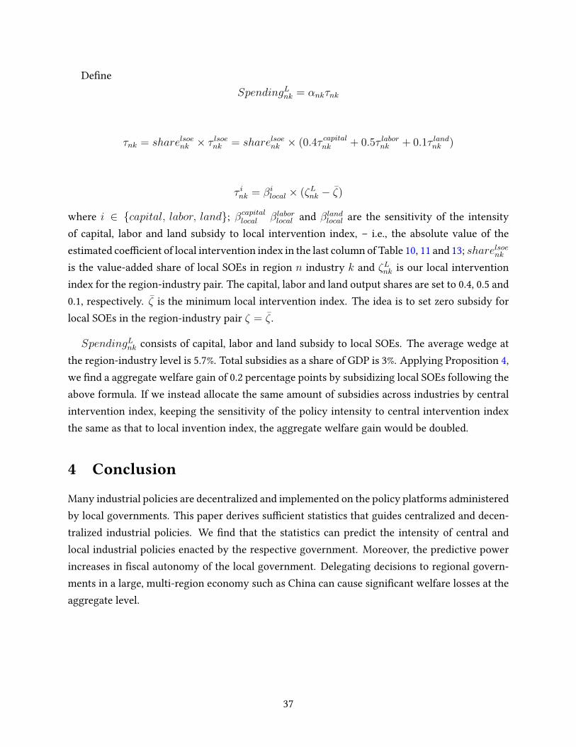
where i ∈ capital, labor, land; βcapitallocal βlaborlocal and βlandlocal are the sensitivity of the intensityof capital, labor and land subsidy to local intervention index, – i.e., the absolute value of theestimated coecient of local intervention index in the last column of Table 10, 11 and 13; sharelsoenk

is the value-added share of local SOEs in region n industry k and ζLnk is our local interventionindex for the region-industry pair. The capital, labor and land output shares are set to 0.4, 0.5 and0.1, respectively. ζ is the minimum local intervention index. The idea is to set zero subsidy forlocal SOEs in the region-industry pair ζ = ζ .

SpendingLnk consists of capital, labor and land subsidy to local SOEs. The average wedge atthe region-industry level is 5.7%. Total subsidies as a share of GDP is 3%. Applying Proposition 4,we nd a aggregate welfare gain of 0.2 percentage points by subsidizing local SOEs following theabove formula. If we instead allocate the same amount of subsidies across industries by centralintervention index, keeping the sensitivity of the policy intensity to central intervention indexthe same as that to local invention index, the aggregate welfare gain would be doubled.

4 Conclusion

Many industrial policies are decentralized and implemented on the policy platforms administeredby local governments. This paper derives sucient statistics that guides centralized and decen-tralized industrial policies. We nd that the statistics can predict the intensity of central andlocal industrial policies enacted by the respective government. Moreover, the predictive powerincreases in scal autonomy of the local government. Delegating decisions to regional govern-ments in a large, multi-region economy such as China can cause signicant welfare losses at theaggregate level.

37

ReferencesAcemoglu, Daron and Pablo D Azar (2020) “Endogenous Production Networks,” Econometrica, 88

(1), 33–82. 1

Bai, Chong-En, Chang-Tai Hsieh, and Zheng Song (2016) “The Long Shadow of China’s FiscalExpansion,” Brookings Papers on Economic Activity, 2016 (2), 129–181. 3.2

(2020a) “Special Deals with Chinese Characteristics,” NBER Macroeconomics Annual, 34(1), 341–379. 1, 3.2, 5, 3.3.3

Bai, Chong-En, Chang-Tai Hsieh, Zheng Song, and Xin Wang (2020b) “Special Deals from SpecialInvestors: The Rise of State-Connected Private Owners in China,” Working paper. 3.2, 3.2.2

Baqaee, David Rezza (2018) “Cascading Failures in Production Networks,” Econometrica, 86 (5),1819–1838. 1

Baqaee, David Rezza and Emmanuel Farhi (2020) “Productivity and Misallocation in General Equi-librium,” The Quarterly Journal of Economics, 135 (1), 105–163. 1, 2.4

Bigio, Saki and Jennifer La’o (2020) “Distortions in Production Networks,” The Quarterly Journalof Economics, 135 (4), 2187–2253. 1

Brandt, Loren, Trevor Tombe, and Xiaodong Zhu (2013) “Factor Market Distortions across Time,Space and Sectors in China,” Review of Economic Dynamics, 16 (1), 39–58. 1

Caliendo, Lorenzo and Fernando Parro (2015) “Estimates of the Trade and Welfare Eects ofNAFTA,” The Review of Economic Studies, 82 (1), 1–44. 1, 2.1, 2.1, 2.2

Dollar, David and Shang-Jin Wei (2007) “Das (Wasted) Kapital: Firm Ownership and InvestmentEciency in China,”Technical report, National Bureau of Economic Research. 1

Hsieh, Chang-Tai and Peter J Klenow (2009) “Misallocation and Manufacturing TFP in China andIndia,” The Quarterly Journal of Economics, 124 (4), 1403–1448. 1, 3.3

Hsieh, Chang-Tai and Zheng Song (2015) “Grasp the Large, Let Go of the Small: The Transforma-tion of the State Sector in China,” Brookings Papers on Economic Activity, 2015 (Spring), 295–346.1, 3.2, 3.3, 3.3.1, 3.3.2

Jones, Charles I (2011) “Intermediate Goods and Weak Links in the Theory of Economic Devel-opment,” American Economic Journal: Macroeconomics, 3 (2), 1–28. 1

38

(2013) “Misallocation, Economic Growth, and Input-Output Economics,” in Advances inEconomics and Econometrics: Tenth World Congress, 2, 419, Cambridge University Press. 1

Kleinman, B., E. Liu, and S. J. Redding (2020) “International Friends and Enemies,” NBER WorkingPaper No. 27587. 2.4

König, Michael, Zheng Song, Kjetil Storesletten, and Fabrizio Zilibotti (2020) “From Imitationto Innovation: Where Is All that Chinese R&D Going?”Technical report, National Bureau ofEconomic Research. 3.2

Li, Hongbin and Li-An Zhou (2005) “Political Turnover and Economic Performance: the IncentiveRole of Personnel Control in China,” Journal of Public Economics, 89 (9-10), 1743–1762. 3.2

Liu, Ernest (2019) “Industrial Policies in Production Networks,” The Quarterly Journal of Eco-nomics, 134 (4), 1883–1948. (document), 1, 2.1, 2.1, 2.4, 3.1, 3.2

Liu, Weidong, Zhipeng Tang, Mengyao Han et al. (2018) “The 2012 China Multi-Regional Input-Output Table of 31 Provincial Units,” The State Council of the People’s Republic of China. 3

Rodrik, Dani (2004) “Industrial Policy for the Twenty-First Century.” 1

Song, Zheng, Kjetil Storesletten, and Fabrizio Zilibotti (2011) “Growing Like China,” AmericanEconomic Review, 101 (1), 196–233. 1, 3.3.1

Song, Zheng and Wei Xiong (2018) “Risks in China’s Financial System,” Annual review of nancialeconomics, 10, 261–286. 3.2

Wang, Yikai (2019) “The Politico-Economic Dynamics of China’s Growth,” Journal of the EuropeanEconomic Association. 1

Wu, Yiyun, Xiwei Zhu, and Nicolaas Groenewold (2019) “The Determinants and Eectivenessof Industrial Policy in China: A Study Based on Five-Year Plans,” China Economic Review, 53,225–242. 1

Xiong, Wei (2018) “The Mandarin Model of Growth,”Technical report, National Bureau of Eco-nomic Research. 1

Xu, Chenggang (2011) “The Fundamental Institutions of China’s Reforms and Development,”Journal of Economic Literature, 49 (4), 1076–1151. 5

39

A Intervention Index

Table A.1: Industry Classication in Input-Output Table: Agriculture and Secondary Sectors

Classication Code 2-Digit Codein IO Table (2011 version)

Farming, Forestry, Animal Production and Fishery 1 1-5Mining and Washing of Coal 2 6Extraction of Crude Petroleum and Natural Gas 3 7Mining of Metal Ores 4 8-9Mining and Quarrying of Nonmetallic Mineral and Other Mineral 5 10-12Manufacture of Food and Tobacco 6 13-16Manufacture of Textiles 7 17Manufacture of Textile Wearing Apparel, Footwear, Leather, Fur, Feather and ItsProducts 8 18-19

Processing of Timbers and Manufacture of Furniture 9 20-21Papermaking, Printing and Manufacture of Articles for Culture, Education andSports Activities 10 22-24

Manufacture of Rened Petroleum, Coke Products, Processing of Nuclear Fuel 11 25Manufacture of Chemicals and Chemical Products 12 26-29Manufacture of Nonmetallic Mineral Products 13 30Manufacture and Processing of Metals 14 31-32Manufacture of Fabricated Metal Products, Except Machinery and Equipment 15 33Manufacture of General-Purpose Machinery 16 34Manufacture of Special-Purpose Machinery 17 35Manufacture of Transport Equipment 18 36-37Manufacture of Electrical Machinery and Apparatus 19 38Manufacture of Communication Equipment, Computer and Other ElectronicEquipment 20 39

Manufacture of Measuring Instruments 21 40Other Manufacture 22 41Scrap and Waste 23 42Repair of Fabricated Metal Products, Machinery and Equipment 24 43Production and Supply of Electricity and Steam 25 44Production and Distribution of Gas 26 45Production and Distribution of Water 27 46Construction 28 47-50

40

Table A.2: Industry Classication in Input-Output Table: Service Sector

Classication Code 2-Digit Codein IO Table (2011 version)

Wholesale and Retail Trade 29 51-52Transport, Storage and Post 30 53-60Accommodation, Food and Beverage Services 31 61-62Information Transmission, Software and Information Technology Services 32 63-65Finance 33 66-69Real Estate 34 70Renting and Leasing, Business Services 35 71-72Scientic Research and Development, Technical Services 36 73-75Management of Water Conservancy, Environment and Public Facilities 37 76-78Services to Households, Repair and Other Services 38 79-81Education 39 82Health Care and Social Work Activities 40 83-84Culture, Sports and Entertainment 41 85-89Public Management, Social Security and Social Organization 42 90-95

Table A.3: Central Intervention Index

(1) (2) (3) (4) (5) (6) (7) (8)

share of sales as local input 0.303∗∗∗ 0.134∗∗∗ 0.282∗∗∗ 0.264∗∗∗ 0.207∗∗∗ 0.227∗∗∗ 0.202∗∗∗ 0.228∗∗∗(0.00863) (0.0122) (0.00776) (0.0130) (0.00599) (0.0108) (0.00582) (0.0108)

share of sales as non-local input 0.397∗∗∗ 0.235∗∗∗ 0.249∗∗∗ 0.199∗∗∗ 0.227∗∗∗ 0.199∗∗∗(0.0235) (0.0168) (0.0128) (0.0122) (0.0115) (0.0122)

index_central 0.832∗∗∗ 0.469∗∗∗ 0.632∗∗∗ 0.471∗∗∗(0.0353) (0.0411) (0.0487) (0.0409)

index_central_nonlocal 0.345∗∗∗ 0.0744(0.0518) (0.0912)

Province Dummy YES YES YES YES YES YES YES YESIndustry Dummy NO YES NO YES NO YES NO YESN 1273 1273 1273 1273 1273 1273 1273 1273R-squared 0.610 0.953 0.820 0.967 0.935 0.981 0.942 0.981Standard errors in parentheses∗ p < 0.1, ∗∗ p < 0.05, ∗∗∗ p < 0.01

Notes: Dependent variables in all the columns are central intervention indices.

41

B State Share: Trimmed Sample

Table B.1: State Share and Intervention Index (trim)

log(central state share) log(local state share)

(1) (2) (3) (4) (5) (6)

central intervention index 2.230∗∗∗ 2.128∗∗∗ 0.885 0.613(0.597) (0.610) (0.539) (0.542)

local intervention index 0.843 0.427 1.210∗∗ 1.084∗∗(0.672) (0.678) (0.501) (0.486)

Province Dummy YES YES YES YES YES YESIndustry Dummy NO NO NO NO NO NON 1048 1048 1048 1111 1111 1111R-squared 0.272 0.253 0.273 0.130 0.137 0.140Standard errors in parentheses∗ p < 0.1, ∗∗ p < 0.05, ∗∗∗ p < 0.01

42

Table B.2: State Share and Intervention Index: Regional Results (trim)

log(central state share) log(local state share)

(1) (2) (3) (4) (5) (6)

Panel A: East

central intervention index 1.313 0.0367 -0.0498 -1.209(0.989) (1.118) (0.903) (0.957)

local intervention index 2.986∗∗ 2.972∗∗ 2.424∗∗ 2.895∗∗∗(1.209) (1.368) (0.956) (0.995)

N 351 351 351 364 364 364R-squared 0.323 0.355 0.355 0.0488 0.0878 0.0958

Panel B: Central

central intervention index 2.884∗∗∗ 3.135∗∗∗ 1.779∗∗ 1.805∗∗(1.080) (1.040) (0.881) (0.864)

local intervention index -0.759 -1.161 -0.0167 -0.169(0.822) (0.720) (0.648) (0.572)

N 214 214 214 218 218 218R-squared 0.161 0.122 0.173 0.219 0.194 0.219

Panel C: West & Northeast

central intervention index 3.282∗∗∗ 3.240∗∗∗ 1.923∗∗∗ 1.895∗∗∗(0.774) (0.787) (0.586) (0.592)

local intervention index -0.969 -0.822 0.564 0.474(0.651) (0.663) (0.527) (0.506)

N 483 483 483 529 529 529R-squared 0.142 0.0764 0.148 0.189 0.153 0.192

Province Dummy YES YES YES YES YES YESIndustry Dummy NO NO NO NO NO NOStandard errors in parentheses∗ p < 0.1, ∗∗ p < 0.05, ∗∗∗ p < 0.01

Notes: East area covers 10 provinces: 4 provinces (Beijing, Tianjin, Hebei and Shandong) in Circum-Bohai-Sea, 3provinces (Shanghai, Jiangsu and Zhejiang) in Yangtze River Delta, and another 3 provinces (Fujian, Guangdong andHainan) in southeastern costal region; Central area includes 6 provinces: Shanxi, Anhui, Jiangxi, Henan, Hubei andHunan; the remaining 15 provinces are in West & Northeast area.

43

Figure B.1: State Share Sensitivity to Intervention Index: Provincial Variation (trim)

44

Figure B.2: Local State Share Sensitivity to Intervention Index: Provincial Variation (trim)

45

C Capital Productivity: Robustness Check

Table C.1: Capital Productivity and Intervention Index 2

(1) (2) (3)

soe_central 0.318∗∗∗ 0.306∗∗∗ 0.322∗∗∗(0.0328) (0.0334) (0.0327)

private 0.667∗∗∗ 0.671∗∗∗ 0.673∗∗∗(0.0262) (0.0260) (0.0259)

central intervention index -0.202 0.0294(0.301) (0.305)

soe_central×central intervention index 0.105 -0.0628(0.365) (0.376)

private×central intervention index 1.156∗∗∗ 0.940∗∗∗(0.219) (0.224)

local intervention index -1.115∗∗∗ -0.999∗∗∗(0.169) (0.176)

soe_central×local intervention index 0.725∗∗∗ 0.757∗∗∗(0.235) (0.247)

private×local intervention index 1.051∗∗∗ 0.918∗∗∗(0.179) (0.187)

Province Dummy YES YES YESIndustry Dummy YES YES YESYear Dummy YES YES YESN 15221 15221 15221R-squared 0.911 0.910 0.911Standard errors in parentheses∗ p < 0.1, ∗∗ p < 0.05, ∗∗∗ p < 0.01

Notes: Dependent variable is log of sales-capital ratio at region-industry-ownership level which is the median valueamong all the rms in each region-industry-ownership group between the year 2011 and 2015; reference group islocal SOEs whose central state share is lower than local state share; dummy variable soe_central equals 1 if it is theregion-industry level sales-capital ratio for SOEs whose central state share is larger than or equal to local state share,otherwise it is 0; dummy variable private equals 1 if it is the region-industry level sales-captial ratio for private rms,otherwise it is 0.

46

D Labor Productivity

D.1 Benchmark Method: No Controls

Table D.1: Labor Productivity and Intervention Index

(1) (2) (3)

soe_central 0.401∗∗∗ 0.385∗∗∗ 0.385∗∗∗(0.0601) (0.0606) (0.0597)

private -0.278∗∗∗ -0.303∗∗∗ -0.302∗∗∗(0.0392) (0.0388) (0.0386)

central intervention index -0.599 -0.420(0.500) (0.480)

soe_central×central intervention index 0.932∗∗ 0.873∗(0.440) (0.453)

private×central intervention index 1.016∗∗∗ 0.883∗∗(0.354) (0.353)

local intervention index -0.932∗∗∗ -0.810∗∗∗(0.208) (0.206)

soe_central×local intervention index 0.433 0.293(0.351) (0.360)

private×local intervention index 0.649∗∗∗ 0.519∗∗(0.223) (0.225)

Province Dummy YES YES YESIndustry Dummy YES YES YESN 3299 3299 3299R-squared 0.888 0.889 0.889Standard errors in parentheses∗ p < 0.1, ∗∗ p < 0.05, ∗∗∗ p < 0.01

Notes: Dependent variable is log of sales-labor ratio at region-industry-ownership level which is the median valueamong all the rms in each region-industry-ownership group between the year 2011 and 2015; reference group islocal SOEs whose central state share is lower than local state share; dummy variable soe_central equals 1 if it is theregion-industry level sales-capital ratio for SOEs whose central state share is larger than or equal to local state share,otherwise it is 0; dummy variable private equals 1 if it is the region-industry level sales-captial ratio for private rms,otherwise it is 0.

47

D.2 Robustness Check

Table D.2: Labor Productivity and Intervention Index: Add Controls 2

(1) (2) (3)

soe_central 0.343∗∗∗ 0.339∗∗∗ 0.345∗∗∗(0.0282) (0.0284) (0.0280)

private 0.109∗∗∗ 0.110∗∗∗ 0.113∗∗∗(0.0272) (0.0270) (0.0270)

central intervention index -0.428 -0.210(0.271) (0.270)

soe_central×central intervention index 0.600∗∗ 0.472∗(0.237) (0.241)

private×central intervention index 1.035∗∗∗ 0.848∗∗∗(0.180) (0.182)

local intervention index -1.072∗∗∗ -0.960∗∗∗(0.119) (0.123)

soe_central×local intervention index 0.657∗∗∗ 0.590∗∗∗(0.184) (0.191)

private×local intervention index 0.892∗∗∗ 0.770∗∗∗(0.138) (0.143)

log(capital intensity) 0.430∗∗∗ 0.428∗∗∗ 0.429∗∗∗(0.0228) (0.0226) (0.0227)

Province Dummy YES YES YESIndustry Dummy YES YES YESYear Dummy YES YES YESN 15221 15221 15221R-squared 0.848 0.848 0.849Standard errors in parentheses∗ p < 0.1, ∗∗ p < 0.05, ∗∗∗ p < 0.01

Notes: Dependent variable is log of sales-labor ratio at region-industry-ownership level which is the median valueamong all the rms in each region-industry-ownership group between the year 2011 and 2015; reference group islocal SOEs whose central state share is lower than local state share; dummy variable soe_central equals 1 if it is theregion-industry level sales-capital ratio for SOEs whose central state share is larger than or equal to local state share,otherwise it is 0; dummy variable private equals 1 if it is the region-industry level sales-captial ratio for private rms,otherwise it is 0; log(capital intensity) is the log of capital-labor ratio at region-industry-ownership level which is themedian value among all the rms in each region-industry-ownership group between the year 2011 and 2015.

48

Table D.3: Labor Productivity and Intervention Index 2

(1) (2) (3)

soe_central 0.417∗∗∗ 0.414∗∗∗ 0.415∗∗∗(0.0303) (0.0306) (0.0304)

private -0.283∗∗∗ -0.283∗∗∗ -0.281∗∗∗(0.0214) (0.0213) (0.0213)

central intervention index -0.546 -0.372(0.333) (0.328)

soe_central×central intervention index 0.852∗∗∗ 0.796∗∗∗(0.234) (0.241)

private×central intervention index 0.971∗∗∗ 0.842∗∗∗(0.188) (0.188)

local intervention index -0.896∗∗∗ -0.780∗∗∗(0.117) (0.119)

soe_central×local intervention index 0.409∗∗ 0.282(0.194) (0.200)

private×local intervention index 0.632∗∗∗ 0.508∗∗∗(0.147) (0.150)

Province Dummy YES YES YESIndustry Dummy YES YES YESYear Dummy YES YES YESN 15221 15221 15221R-squared 0.800 0.801 0.801Standard errors in parentheses∗ p < 0.1, ∗∗ p < 0.05, ∗∗∗ p < 0.01

Notes: Dependent variable is log of sales-labor ratio at region-industry-ownership level which is the median valueamong all the rms in each region-industry-ownership group between the year 2011 and 2015; reference group islocal SOEs whose central state share is lower than local state share; dummy variable soe_central equals 1 if it is theregion-industry level sales-capital ratio for SOEs whose central state share is larger than or equal to local state share,otherwise it is 0; dummy variable private equals 1 if it is the region-industry level sales-captial ratio for private rms,otherwise it is 0.

49

E Land Productivity

E.1 Benchmark Method: No Controls

Table E.1: Land Productivity and Intervention Index

(1) (2) (3)

soe_central 0.400∗∗∗ 0.389∗∗∗ 0.374∗∗∗(0.0764) (0.0746) (0.0741)

private 0.252∗∗∗ 0.218∗∗∗ 0.216∗∗∗(0.0543) (0.0518) (0.0520)

central intervention index 0.734 0.933(0.579) (0.588)

soe_central×central intervention index 1.277∗∗ 1.158∗(0.619) (0.642)

private×central intervention index 0.762∗ 0.559(0.429) (0.430)

local intervention index -1.108∗∗∗ -1.040∗∗∗(0.348) (0.365)

soe_central×local intervention index 0.713 0.527(0.571) (0.587)

private×local intervention index 0.873∗∗ 0.811∗∗(0.354) (0.373)

Province Dummy YES YES YESIndustry Dummy YES YES YESN 3116 3116 3116R-squared 0.894 0.893 0.894Standard errors in parentheses∗ p < 0.1, ∗∗ p < 0.05, ∗∗∗ p < 0.01

Notes: Dependent variable is log of sales-land ratio at region-industry-ownership level which is the median valueamong all the rms in each region-industry-ownership group between the year 2011 and 2015; reference group islocal SOEs whose central state share is lower than local state share; reference group is local SOEs whose centralstate share is lower than local state share; dummy variable soe_central equals 1 if it is the region-industry level sales-capital ratio for SOEs whose central state share is larger than or equal to local state share, otherwise it is 0; dummyvariable private equals 1 if it is the region-industry level sales-captial ratio for private rms, otherwise it is 0.

50

E.2 Robustness Check

Table E.2: Land Productivity and Intervention Index: Add Controls 2

(1) (2) (3)

soe_central 0.446∗∗∗ 0.460∗∗∗ 0.445∗∗∗(0.0386) (0.0389) (0.0388)

private 0.177∗∗∗ 0.183∗∗∗ 0.181∗∗∗(0.0289) (0.0285) (0.0286)

central intervention index 0.803∗∗ 1.006∗∗∗(0.315) (0.319)

soe_central×central intervention index 1.388∗∗∗ 1.282∗∗∗(0.311) (0.322)

private×central intervention index 0.820∗∗∗ 0.613∗∗∗(0.230) (0.230)

local intervention index -1.121∗∗∗ -1.047∗∗∗(0.194) (0.201)

soe_central×local intervention index 0.700∗∗ 0.493(0.304) (0.311)

private×local intervention index 0.900∗∗∗ 0.833∗∗∗(0.197) (0.206)

log(capital intensity) -0.126∗∗∗ -0.122∗∗∗ -0.126∗∗∗(0.0216) (0.0216) (0.0216)

Province Dummy YES YES YESIndustry Dummy YES YES YESYear Dummy YES YES YESN 13927 13927 13927R-squared 0.850 0.849 0.851Standard errors in parentheses∗ p < 0.1, ∗∗ p < 0.05, ∗∗∗ p < 0.01

Notes: Dependent variable is log of sales-land ratio at region-industry-ownership level which is the median valueamong all the rms in each region-industry-ownership group between the year 2011 and 2015; reference group islocal SOEs whose central state share is lower than local state share; dummy variable soe_central equals 1 if it is theregion-industry level sales-capital ratio for SOEs whose central state share is larger than or equal to local state share,otherwise it is 0; dummy variable private equals 1 if it is the region-industry level sales-captial ratio for private rms,otherwise it is 0; log(capital intensity) is the log of capital-labor ratio at region-industry-ownership level which is themedian value among all the rms in each region-industry-ownership group between the year 2011 and 2015.

51

Table E.3: Land Productivity and Intervention Index 2

(1) (2) (3)

soe_central 0.429∗∗∗ 0.442∗∗∗ 0.429∗∗∗(0.0385) (0.0388) (0.0387)

private 0.229∗∗∗ 0.232∗∗∗ 0.233∗∗∗(0.0284) (0.0281) (0.0281)

central intervention index 0.720∗∗ 0.912∗∗∗(0.316) (0.320)

soe_central×central intervention index 1.312∗∗∗ 1.196∗∗∗(0.324) (0.336)

private×central intervention index 0.840∗∗∗ 0.643∗∗∗(0.229) (0.230)

local intervention index -1.088∗∗∗ -1.009∗∗∗(0.191) (0.199)

soe_central×local intervention index 0.703∗∗ 0.511(0.303) (0.312)

private×local intervention index 0.857∗∗∗ 0.784∗∗∗(0.195) (0.204)

Province Dummy YES YES YESIndustry Dummy YES YES YESYear Dummy YES YES YESN 13927 13927 13927R-squared 0.848 0.848 0.849Standard errors in parentheses∗ p < 0.1, ∗∗ p < 0.05, ∗∗∗ p < 0.01

Notes: Dependent variable is log of sales-land ratio at region-industry-ownership level which is the median valueamong all the rms in each region-industry-ownership group between the year 2011 and 2015; reference group islocal SOEs whose central state share is lower than local state share; dummy variable soe_central equals 1 if it is theregion-industry level sales-capital ratio for SOEs whose central state share is larger than or equal to local state share,otherwise it is 0; dummy variable private equals 1 if it is the region-industry level sales-captial ratio for private rms,otherwise it is 0.

52