Int. J. Production Economics 146 (2013) 269–280

Contents lists available at ScienceDirect

Int. J. Production Economics

0925-52http://d

n CorrE-m

journal homepage: www.elsevier.com/locate/ijpe

Decision analysis on CDM project investments

Jing Li n, Navid SabbaghiIllinois Institute of Technology, Stuart School of Business, Chicago, IL 60661, United States

a r t i c l e i n f o

Article history:Received 21 January 2013Accepted 11 July 2013Available online 24 July 2013

Keywords:Clean Development Mechanism (CDM)Project financeCDM contractsKyoto Protocol

73/$ - see front matter & 2013 Elsevier B.V. Ax.doi.org/10.1016/j.ijpe.2013.07.010

esponding author. Tel.: +1 3128235680.ail addresses: jli64@iit.edu (J. Li), nsabbagh@s

a b s t r a c t

The Clean Development Mechanism (CDM) is a mechanism defined in the Kyoto protocol thatincentivizes parties to the protocol to fund sustainable development projects in countries that are notparty to the protocol. We analyze a target contract financing structure for different CDM projects in orderto see under what conditions the financing structure is efficient and to explore the contract's allocation ofprofit among the firms. In the two broad categories of CDM projects we consider, we find the optimalinvestment decision for the investor and for the overall system. We also analyze how the residual valueof technology would affect the financing, target contract's efficiency and allocation of profit.

& 2013 Elsevier B.V. All rights reserved.

1. Introduction

The United Nations Framework Convention on Climate Changepromotes the Clean Development Mechanism (CDM) as a meansfor firms in developed nations that are regulated under a cap andtrade program to obtain greenhouse gas (GHG) certified emissionreduction (CER) credits for the program by financing GHG reduc-tion projects in developing nations. There are a number of waysthese CDM projects are financed. For example, a financier couldprovide project finance to a hydro electricity generation CDMproject in Central America and receive CERs as repayment for afixed proportion of the interest on the loan. Then, the financiercould sell CERs to firms in Europe that are regulated under the EUemissions trading scheme. Alternatively, an investor could financea CDM project using equity and ask for a share in the CERsgenerated by the CDM project. Technology swaps are also usedto finance CDM projects. As an example, a Spanish companyprovides new renewable energy technology to a CDM project inChina, which would otherwise incur significant licensing fees, inexchange for the CERs that the project generates. An importantquestion in this context is: how efficient are these financingarrangements? And which financing arrangement is moreefficient?

In this paper we focus on target contracts in which the projectrepays the investor with a target number of CER credits, if they aregenerated. Due to the uncertainty in the number of CER creditsgenerated, the investor receives an uncertain repayment for theguaranteed investment amount. We assume the investor andproject are risk neutral and assess the efficiency for these

ll rights reserved.

tuart.iit.edu (N. Sabbaghi).

contracts. Furthermore, we analyze the profit allocation betweenthe firms when utilizing such contracts.

The UNFCCC has distinguished more than ten categories ofCDM project based on the nature of the project. More than half ofCDM projects are in renewable energy sector, such as wind, hydro,biomass, solar, and produce energy, in addition to CER credits.However, significant amount of CERs are generated in the sectorthat projects reduce HFC and PFC gases and produce no particulargood. Therefore, we classify CDM projects into two categoriesaccording to whether or not CERs are the only output.

The next section reviews the related literature. Section 3describes the model in greater detail. Section 4 provides theanalysis and Section 5 discusses the conclusions.

2. Literature review

UNEP (2004) provides the background on CDM projects, rolesof key participants, the legal steps in developing a CDM project,key legal requirements for a qualified CDM project, and introducesto features of CERs. It also briefly introduces the financing,structuring, and management of CDM projects. UNEP (2007)focuses on the financing and structuring of CDM projects. Severalsuccessful CDM cases are studied and many details are providedabout different financing structures. The examples in this bookmotivate the model and analysis in our paper, which can representboth HFC projects and wind farm projects. There is no academicliterature addressing CDM project financing, and the efficiency oftarget contracts. Also, World Bank (Alexandre and Guigon, 2012)provides yearly updates and trends on CDM projects.

Esty (2002, 2003, 2007) define, analyze and summarize proper-ties of project finance through a series papers. Esty (2002)demonstrates how project finance creates value and the motivates

J. Li, N. Sabbaghi / Int. J. Production Economics 146 (2013) 269–280270

when it should be used rather than other financing methods. Esty(2003) shows how project financing out-performed corporatefinancing through reducing both agency conflicts and under-investment. Esty (2007) gives a more precise definition and thelatest trend of project finance.

Esty (2003) illustrates the main structural components ofproject finance: organizational structure, capital structure, owner-ship structure, board structure, and contract structure. However,existing research for project finance concentrates in the areas ofcapital structure and ownership structure. For example, in the areaof capital structure, Shah and Thakor (1987) provide a model toexplain higher leverage in project financing. John and John (1991)provide related results. In the area of ownership structure, themain focus is on the syndicated bank loan and its nonrecoursecharacter. Berkovitch and HanKim (1990), Flannery et al. (1993),Marco and Gadanecz (2008), and Benjamin and Megginson (2003)study how project finance outperforms corporate finance throughnonrecourse debt.

There is very little literature in the area of contract structure forproject finance, which is the topic of this paper. Sometimes projectfinance is referred to as contract finance because the contractualstructure of a project is an important project component accordingto Esty's definition. Jensen and Meckling (1976) view a firm as acombination of contracting relationships. Brealey et al. (1996)explain in detail how the complex combination of contracts andfinancing arrangements in project finance distributes risk amongthe parties. Furthermore, Francesco et al. (2010) empirically studyhow the network of contracts affects the loan spread and capitalstructure.

Our study is motivated by the scant attention paid to the CDMproject and project finance. Current research in CDM projects ismainly through perspectives of law and policy, not from econom-ics and finance. Our paper attempts to contribute in the followingways. First, despite the rapid growth in CDM projects as reportedby the World Bank, to the best of our knowledge, this is the onlypaper that studies CDM project financing. Second, our paper is anapplication of project finance to a new area rather than to oil, gas,and infrastructure projects. In addition, project finance involves anetwork of contracts among participants as mentioned in previouspapers. We provide a detailed analysis of the contracts between aninvestor and the project company. Working through models underdifferent conditions, we demonstrate how the design of thecontract would eventually affect the efficiency, profits, and socialwelfare of both parties.

3. Model

The main participants in project finance include the projectcompany, supplier(s), project sponsor(s), lenders and other inves-tors, customer(s), government, and contractor(s) (Brealey et al.,1996).1 We provide a stylized model that considers two of themain participants: the project company and the investor.

Consider a two period model with one investor i that considersfinancing a CDM project s. In the first period, the investor invests xin the CDM project, for example, enabling the project to purchasetechnology that generates CER credits. As a result, the technologyinvestment x generates a random yield Q(x) of emission reductioncredits in the second period. We suppose the random variable Q(x)has a cumulative distribution function (c.d.f.) F parameterized bythe investment level x and probability distribution function (p.d.f.)f. We assume that every realization of the random function Q(x) is

1 CDM projects have additional participants such as the Designated NationalAuthority and CDM Executive Board that monitor the project.

concave in the investment level x. In the second period, we assumethe market price for credits is known to be p per unit credit andthe technology purchased retains a fraction α of its original value x.The CDM project faces a cost c to produce one emission reductioncredit, for example, because of the raw materials needed toproduce each credit and for verifying or registering the creditswith the governing body of the CDM. The technology α decidesthe residual revenue that CDM project could take. In particular, thetechnology is assumed to be useful for a finite time horizonafter which the technology can be sold for α fraction of it'soriginal value.

In this paper, we study a negotiation setting, not a StackelbergGame. In particular, we do not specify which parties chose thedecision variables, instead we want determine which decisions areefficient. For simplicity, we do not consider the details of theinvestment, such as the debt-to-equity ratio or the syndication ofthe loan.

As mentioned in Section 1, based on the characteristics of CDMprojects, there are two main categories depending on whether ornot there are other underlying outputs other than the CERs.Within each of these main categories, there may or may not bedemand uncertainty for the CERs, depending on whether or not aCER buyer has already been found. Therefore, we initially assumethe investor can sell any amount of CERs at the market price p. Thisassumption is relaxed later to let the investor face a marketdemand for CERs. Based on these observations and assumptions,we create and analyze four models in the following sections.

3.1. Projects without underlying products and without demanduncertainty for CERs

If we consider the investor and the CDM project to be one firm,then the overall system's problem is to choose the non-negativeinvestment level x that maximizes the overall expected profit

ΠðxÞ ¼ ðp�cÞE½Q ðxÞ��ð1�αÞx: ð1ÞThe investor's problem in the first period is to choose the

investment level x given a target number of credits q and promiseddelivery of minðq;Q ðxÞÞ credits in the second period in order tomaximize the expected profit

πiðq; xÞ ¼ pE½minðq;Q ðxÞÞ��x: ð2ÞGiven a target number of credits q the project aims to deliver

to the investor and given investment level x, the CDM project'sprofit is

πsðq; xÞ ¼ αxþ ðp�cÞE½Q ðxÞ��pE½minðq;Q ðxÞÞ�: ð3ÞIn this case, we assume that the only output of the developer is

CER, which is corresponding to the HFC decomposition sector.

3.2. Projects without underlying products and with demanduncertainty for CERs

In this setting we no longer assume that investor can sell all Q(x) credits, rather investor have an uncertain demand D foremission reduction credits that can be sold at price p. Supposethe random variable D has c.d.f. FD and p.d.f. fD. We assume thatthe demand for credits D is independent of the yield Q(x).Generalizing Eq. (1), the overall system's problem is to choosethe investment level x that maximizes the overall expected profit

ΠðxÞ ¼ pE½minðQ ðxÞ;DÞ��cE½Q ðxÞ��ð1�αÞx: ð4ÞIn the first period, given a target quantity of credits q to be

delivered to the investor, uncertain demand D for emissionreduction credits, and promised delivery of minðq;Q ðxÞÞ creditsin the second period, the investor chooses the investment level x

J. Li, N. Sabbaghi / Int. J. Production Economics 146 (2013) 269–280 271

in order to maximize the profit

πiðq; xÞ ¼ pE½minðq;Q ðxÞ;DÞ��x: ð5ÞTherefore, given a target quantity of credits q that the project

aims to deliver to the investor and given investment level x, theCDM project's profit becomes

πsðq; xÞ ¼ αxþ pE½minðQ ðxÞ;DÞ��pE½minðq;Q ðxÞ;DÞ��cE½Q ðxÞ�: ð6Þ

3.3. Projects with underlying products and without demanduncertainty for CERs

In this model, as a result of the underlying technology invest-ment x, there is an additional underlying product produced inaddition to the CERs generated. For example, if the technologyinvestment finances a clean energy project there is also electricityproduced in addition to the CERs generated. We assume that thequantity of underlying product U(x) is a function of the investmentlevel x and linearly related to the emission reduction credits.Namely, for some constant λ, suppose UðxÞ ¼ λQ ðxÞ. Furthermore,we assume that the underlying product can be sold in the marketat price m per unit. Therefore, generalizing Eq. (1), the system'sproblem is to choose the investment level x that maximizes theoverall expected profit

ΠðxÞ ¼ ðpþmλ�cÞE½Q ðxÞ��ð1�αÞx: ð7ÞAs in the previous model, the investor chooses the investment

level x in order to maximize the profit

πiðq; xÞ ¼ pE½minðq;Q ðxÞÞ��x: ð8ÞThe CDM project's profit becomes

πsðq; xÞ ¼ αxþ ðpþmλ�cÞE½Q ðxÞ��pE½minðq;Q ðxÞÞ�: ð9Þ

3.4. Projects with underlying products and with demand uncertaintyfor CERs

Now we combine the assumptions in the previous two modelsand assume that at price p we have an uncertain demand D foremission reduction credits and we have a quantity λQ ðxÞ of anunderlying product that we can sell at price m. Generalizing Eq.(7), the system's problem is to choose the investment level x thatmaximizes the overall expected profit

ΠðxÞ ¼ pE½minQ ðxÞ;D� þ ðmλ�cÞE½Q ðxÞ��ð1�αÞx: ð10ÞThe investor chooses the investment level x in order to

maximize the profit

πiðq; xÞ ¼ pE½minðq;Q ðxÞ;DÞ��x: ð11ÞAnd the CDM project's profit is

πsðq; xÞ ¼ αxþ pE½minðQ ðxÞ;DÞ� þ ðmλ�cÞE½Q ðxÞ��pE½minðq;Q ðxÞ;DÞ�: ð12Þ

3.5. Efficiency and profit allocation

For each model, we denote the optimal investment amount forthe overall system by

xo ¼ arg maxx

ΠðxÞ: ð13Þ

Furthermore, for a given target q we denote the investor'soptimal investment by

xnðqÞ ¼ arg maxx

πiðq; xÞ: ð14Þ

The CDM financing contract is efficient when the investor hasan incentive to invest the system optimal amount, i.e., xnðqÞ ¼ xo.

We are only interested in target contracts q that allow both theproject and the investor to make a non-negative profit. As a result,

the only target contracts of interest are the contracts q in the set

I ¼ fqjπiðq; xnðqÞÞ≥0; πsðq; xnðqÞÞ≥0g ð15Þbecause they are incentive compatible for both the project andinvestor.

For a target contract q∈I , we define the efficiency EffðqÞ of thecontract as the fraction of system optimal profit that the contract qinduces, i.e.,

Eff qð Þ ¼ ΠðxnðqÞÞΠðxoÞ : ð16Þ

In the following analysis, in addition to considering the efficiencyof a target contract q, we also analyze the fraction of profitallocated to the investor

πiðq; xnðqÞÞΠðxnðqÞÞ ð17Þ

and similarly to the project.For any contract q to which the parties agree, Eq. (16) provides

a measure of the social welfare. If the efficiency is 1, the contractcaptures the largest possible profit for the two parties. Otherwise,the profit for the participants as a whole can be increased. Also in acompetitive setting, incentives are aligned so that the efficientcontract is not chosen, in which case the efficiency is less than 1. Inaddition, the contract setting will decide how the profit isallocated between the parties, as defined through Eq. (17).

4. Analysis

4.1. Projects without underlying products and without demanduncertainty for CERs

Our first result describes the set of targets contracts q thatmotivate the investor to invest the system optimal amount.

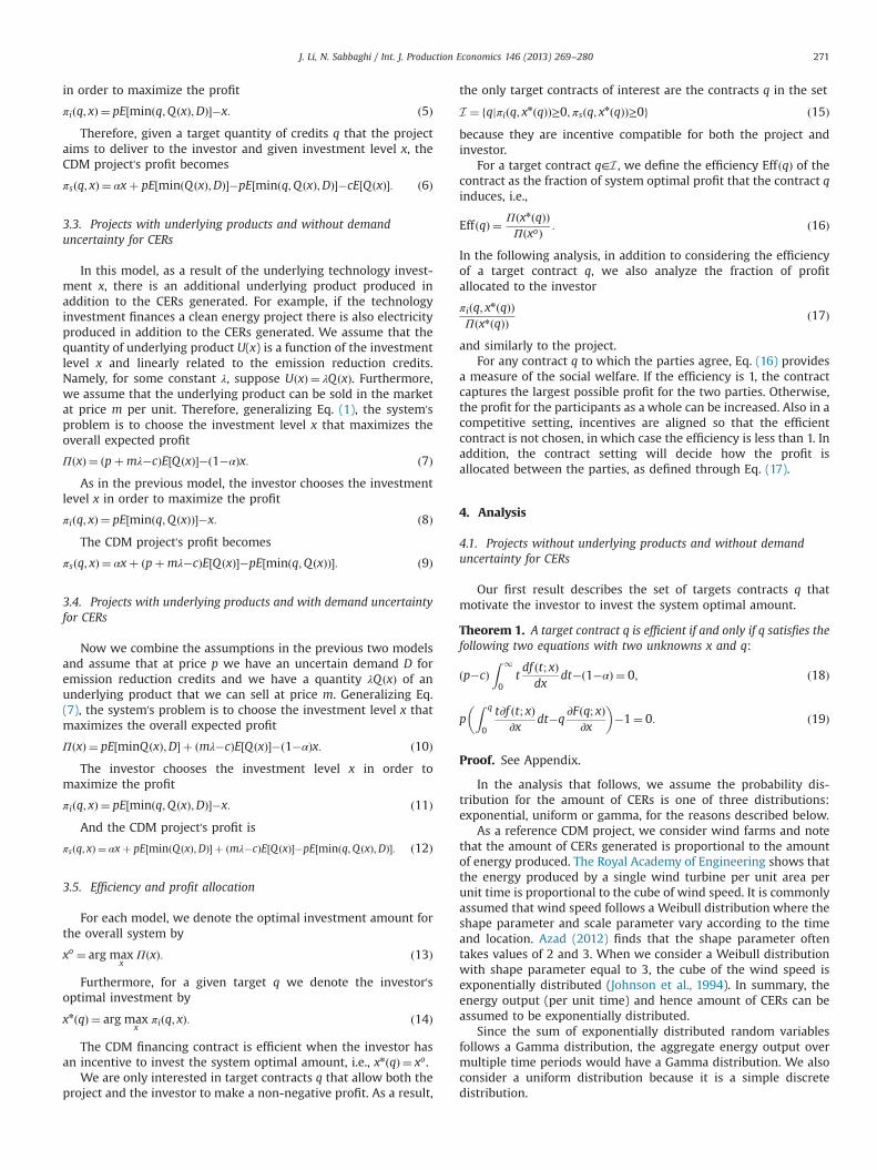
Theorem 1. A target contract q is efficient if and only if q satisfies thefollowing two equations with two unknowns x and q:

p�cð ÞZ 1

0tdf ðt; xÞdx

dt� 1�αð Þ ¼ 0; ð18Þ

pZ q

0

t∂f ðt; xÞ∂x

dt�q∂Fðq; xÞ

∂x

� ��1¼ 0: ð19Þ

Proof. See Appendix.

In the analysis that follows, we assume the probability dis-tribution for the amount of CERs is one of three distributions:exponential, uniform or gamma, for the reasons described below.

As a reference CDM project, we consider wind farms and notethat the amount of CERs generated is proportional to the amountof energy produced. The Royal Academy of Engineering shows thatthe energy produced by a single wind turbine per unit area perunit time is proportional to the cube of wind speed. It is commonlyassumed that wind speed follows a Weibull distribution where theshape parameter and scale parameter vary according to the timeand location. Azad (2012) finds that the shape parameter oftentakes values of 2 and 3. When we consider a Weibull distributionwith shape parameter equal to 3, the cube of the wind speed isexponentially distributed (Johnson et al., 1994). In summary, theenergy output (per unit time) and hence amount of CERs can beassumed to be exponentially distributed.

Since the sum of exponentially distributed random variablesfollows a Gamma distribution, the aggregate energy output overmultiple time periods would have a Gamma distribution. We alsoconsider a uniform distribution because it is a simple discretedistribution.

J. Li, N. Sabbaghi / Int. J. Production Economics 146 (2013) 269–280272

4.1.1. Exponential distributionSuppose that for a fixed investment x the random variable Q(x)

has an exponential distribution with meanffiffiffix

p. In particular, the c.

d.f. for Q(x) is Fðt; xÞ ¼ 1�eð�1=ffiffix

p Þt when t≥0 and Fðt; xÞ ¼ 0 other-wise. And the p.d.f. is f ðt; xÞ ¼ 1=

ffiffiffix

peð�1=

ffiffix

p Þt when t≥0 andf ðt; xÞ ¼ 0 otherwise.

Solving the equation dΠðxoÞ=dx¼ 0 for the socially optimalinvestment xo, we have from Eq. (18) that

xo ¼ p�c2ð1�αÞ

� �2

: ð20Þ

Observe that as the remaining fractional value α or the margin p�cincreases, we have that the optimal investment also increases. Forexample, if the residual value of technology at the end of timehorizon increases or if the developer's cost decreases, then theoptimal social investment increases.

Furthermore, from Eq. (19), we have that for any target contractq, the investor's optimal investment xn (under exponential dis-tribution) satisfies the equation

p � �12

�1þ e�q=ffiffiffiffixn

pþ qffiffiffiffiffi

xnp e�q=

ffiffiffiffixn

p

ffiffiffiffiffixn

p

0B@

1CA�1¼ 0 ð21Þ

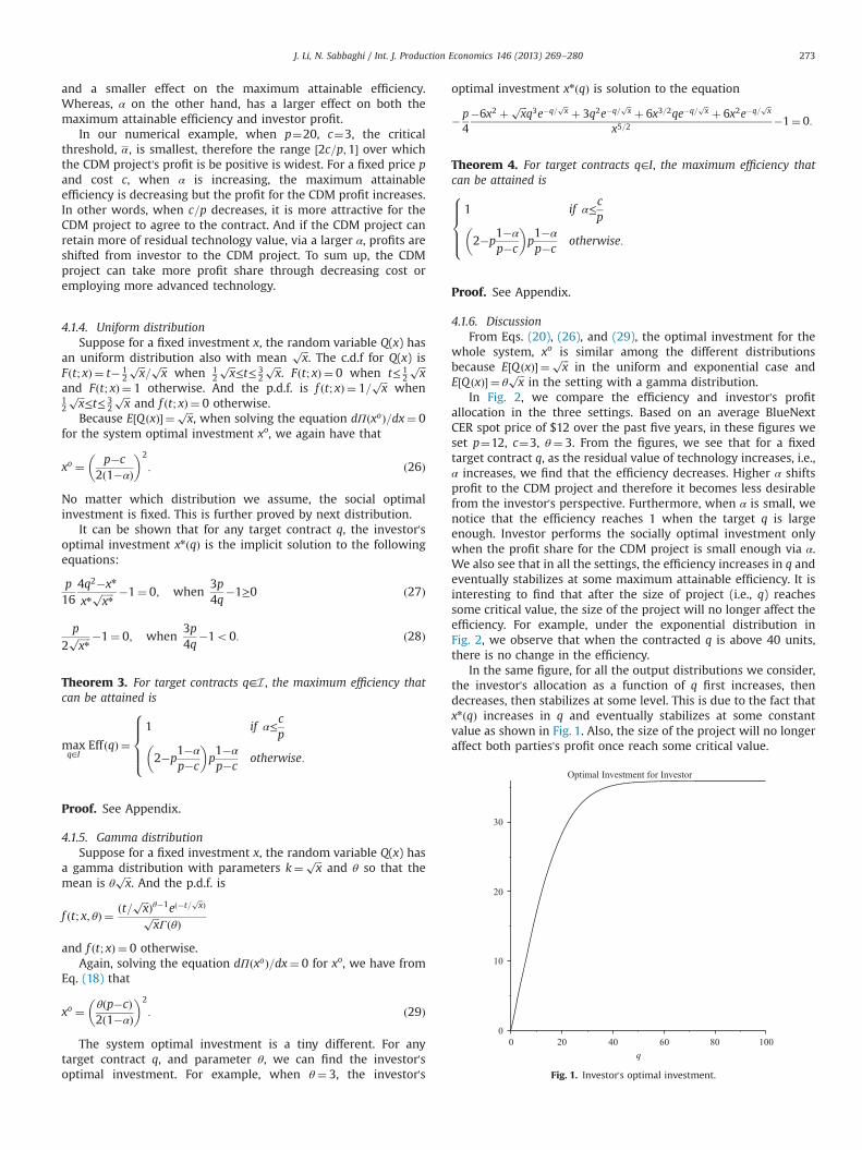
Although the explicit form of xn is difficult to write down, Fig. 1shows the relationship of xn with intended amount q. We chosethe price p¼12 based on an average BlueNext CER spot price of$12 over the past five years.

According to the definition of efficiency in Eq. (16), the contractwould be efficient when xo found in Eq. (20) satisfies the investor'sfirst order condition in Eq. (21), which leads to the followingequation.

p � �12

�1þ e�q=ffiffiffiffixo

pþ qffiffiffiffiffi

xop e�q=

ffiffiffiffixo

p

ffiffiffiffiffixo

p

0B@

1CA�1¼ 0: ð22Þ

4.1.2. Efficiency

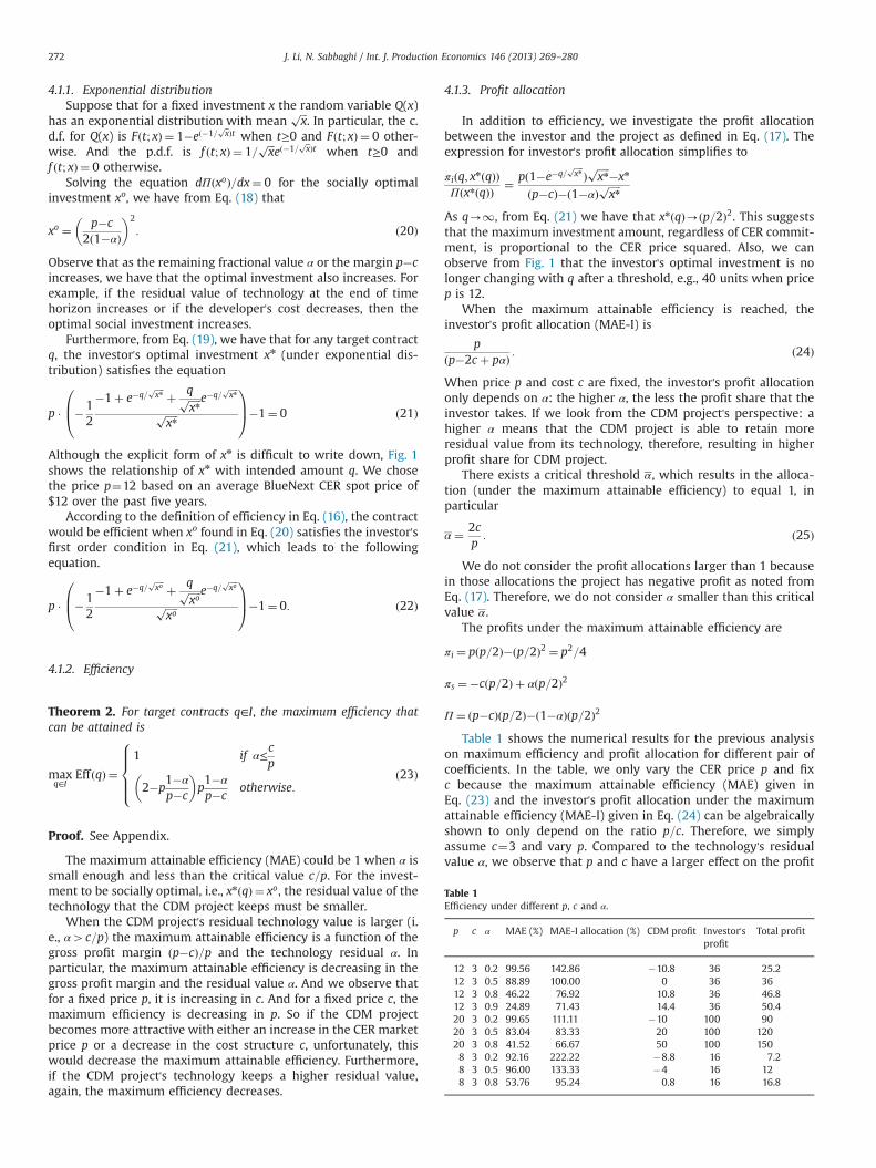
Table 1Efficiency under different p, c and α.

p c α MAE (%) MAE-I allocation (%) CDM profit Investor'sprofit

Total profit

12 3 0.2 99.56 142.86 �10.8 36 25.212 3 0.5 88.89 100.00 0 36 3612 3 0.8 46.22 76.92 10.8 36 46.812 3 0.9 24.89 71.43 14.4 36 50.420 3 0.2 99.65 111.11 �10 100 9020 3 0.5 83.04 83.33 20 100 12020 3 0.8 41.52 66.67 50 100 1508 3 0.2 92.16 222.22 �8.8 16 7.28 3 0.5 96.00 133.33 �4 16 128 3 0.8 53.76 95.24 0.8 16 16.8

Theorem 2. For target contracts q∈I, the maximum efficiency thatcan be attained is

maxq∈I

Eff qð Þ ¼1 if α≤

cp

2�p1�α

p�c

� �p1�α

p�cotherwise:

8>>><>>>:

ð23Þ

Proof. See Appendix.

The maximum attainable efficiency (MAE) could be 1 when α issmall enough and less than the critical value c=p. For the invest-ment to be socially optimal, i.e., xnðqÞ ¼ xo, the residual value of thetechnology that the CDM project keeps must be smaller.

When the CDM project's residual technology value is larger (i.e., α4c=p) the maximum attainable efficiency is a function of thegross profit margin ðp�cÞ=p and the technology residual α. Inparticular, the maximum attainable efficiency is decreasing in thegross profit margin and the residual value α. And we observe thatfor a fixed price p, it is increasing in c. And for a fixed price c, themaximum efficiency is decreasing in p. So if the CDM projectbecomes more attractive with either an increase in the CER marketprice p or a decrease in the cost structure c, unfortunately, thiswould decrease the maximum attainable efficiency. Furthermore,if the CDM project's technology keeps a higher residual value,again, the maximum efficiency decreases.

4.1.3. Profit allocation

In addition to efficiency, we investigate the profit allocationbetween the investor and the project as defined in Eq. (17). Theexpression for investor's profit allocation simplifies to

πiðq; xnðqÞÞΠðxnðqÞÞ ¼ pð1�e�q=

ffiffiffiffixn

pÞffiffiffiffiffixn

p�xn

ðp�cÞ�ð1�αÞffiffiffiffiffixn

p

As q-1, from Eq. (21) we have that xnðqÞ-ðp=2Þ2. This suggeststhat the maximum investment amount, regardless of CER commit-ment, is proportional to the CER price squared. Also, we canobserve from Fig. 1 that the investor's optimal investment is nolonger changing with q after a threshold, e.g., 40 units when pricep is 12.

When the maximum attainable efficiency is reached, theinvestor's profit allocation (MAE-I) is

pðp�2c þ pαÞ : ð24Þ

When price p and cost c are fixed, the investor's profit allocationonly depends on α: the higher α, the less the profit share that theinvestor takes. If we look from the CDM project's perspective: ahigher α means that the CDM project is able to retain moreresidual value from its technology, therefore, resulting in higherprofit share for CDM project.

There exists a critical threshold α , which results in the alloca-tion (under the maximum attainable efficiency) to equal 1, inparticular

α ¼ 2cp: ð25Þ

We do not consider the profit allocations larger than 1 becausein those allocations the project has negative profit as noted fromEq. (17). Therefore, we do not consider α smaller than this criticalvalue α .

The profits under the maximum attainable efficiency are

πi ¼ pðp=2Þ�ðp=2Þ2 ¼ p2=4

πs ¼�cðp=2Þ þ αðp=2Þ2

Π ¼ ðp�cÞðp=2Þ�ð1�αÞðp=2Þ2

Table 1 shows the numerical results for the previous analysison maximum efficiency and profit allocation for different pair ofcoefficients. In the table, we only vary the CER price p and fixc because the maximum attainable efficiency (MAE) given inEq. (23) and the investor's profit allocation under the maximumattainable efficiency (MAE-I) given in Eq. (24) can be algebraicallyshown to only depend on the ratio p=c. Therefore, we simplyassume c¼3 and vary p. Compared to the technology's residualvalue α, we observe that p and c have a larger effect on the profit

J. Li, N. Sabbaghi / Int. J. Production Economics 146 (2013) 269–280 273

and a smaller effect on the maximum attainable efficiency.Whereas, α on the other hand, has a larger effect on both themaximum attainable efficiency and investor profit.

In our numerical example, when p¼20, c¼3, the criticalthreshold, α , is smallest, therefore the range ½2c=p;1� over whichthe CDM project's profit is be positive is widest. For a fixed price pand cost c, when α is increasing, the maximum attainableefficiency is decreasing but the profit for the CDM profit increases.In other words, when c=p decreases, it is more attractive for theCDM project to agree to the contract. And if the CDM project canretain more of residual technology value, via a larger α, profits areshifted from investor to the CDM project. To sum up, the CDMproject can take more profit share through decreasing cost oremploying more advanced technology.

Fig. 1. Investor's optimal investment.

4.1.4. Uniform distributionSuppose for a fixed investment x, the random variable Q(x) has

an uniform distribution also with meanffiffiffix

p. The c.d.f for Q(x) is

F t; xð Þ ¼ t� 12

ffiffiffix

p=ffiffiffix

pwhen 1

2

ffiffiffix

p≤t≤ 3

2

ffiffiffix

p. Fðt; xÞ ¼ 0 when t≤ 1

2

ffiffiffix

p

and Fðt; xÞ ¼ 1 otherwise. And the p.d.f. is f ðt; xÞ ¼ 1=ffiffiffix

pwhen

12

ffiffiffix

p≤t≤ 3

2

ffiffiffix

pand f ðt; xÞ ¼ 0 otherwise.

Because E½Q ðxÞ� ¼ ffiffiffix

p, when solving the equation dΠðxoÞ=dx¼ 0

for the system optimal investment xo, we again have that

xo ¼ p�c2ð1�αÞ

� �2

: ð26Þ

No matter which distribution we assume, the social optimalinvestment is fixed. This is further proved by next distribution.

It can be shown that for any target contract q, the investor'soptimal investment xnðqÞ is the implicit solution to the followingequations:

p16

4q2�xn

xnffiffiffiffiffixn

p �1¼ 0; when3p4q

�1≥0 ð27Þ

p2ffiffiffiffiffixn

p �1¼ 0; when3p4q

�1o0: ð28Þ

Theorem 3. For target contracts q∈I , the maximum efficiency thatcan be attained is

maxq∈I

Eff qð Þ ¼1 if α≤

cp

2�p1�α

p�c

� �p1�α

p�cotherwise:

8>>><>>>:

Proof. See Appendix.

4.1.5. Gamma distributionSuppose for a fixed investment x, the random variable Q(x) has

a gamma distribution with parameters k¼ ffiffiffix

pand θ so that the

mean is θffiffiffix

p. And the p.d.f. is

f t; x; θð Þ ¼ ðt= ffiffiffix

p Þθ�1eð�t=ffiffix

p Þffiffiffix

pΓðθÞ

and f ðt; xÞ ¼ 0 otherwise.Again, solving the equation dΠðxoÞ=dx¼ 0 for xo, we have from

Eq. (18) that

xo ¼ θðp�cÞ2ð1�αÞ

� �2

: ð29Þ

The system optimal investment is a tiny different. For anytarget contract q, and parameter θ, we can find the investor'soptimal investment. For example, when θ¼ 3, the investor's

optimal investment xnðqÞ is solution to the equation

� p4�6x2 þ ffiffiffi

xp

q3e�q=ffiffix

pþ 3q2e�q=

ffiffix

pþ 6x3=2qe�q=

ffiffix

pþ 6x2e�q=

ffiffix

p

x5=2�1¼ 0:

Theorem 4. For target contracts q∈I, the maximum efficiency thatcan be attained is

1 if α≤cp

2�p1�α

p�c

� �p1�α

p�cotherwise:

8>>><>>>:

Proof. See Appendix.

4.1.6. DiscussionFrom Eqs. (20), (26), and (29), the optimal investment for the

whole system, xo is similar among the different distributionsbecause E½Q ðxÞ� ¼ ffiffiffi

xp

in the uniform and exponential case andE½Q ðxÞ� ¼ θ

ffiffiffix

pin the setting with a gamma distribution.

In Fig. 2, we compare the efficiency and investor's profitallocation in the three settings. Based on an average BlueNextCER spot price of $12 over the past five years, in these figures weset p¼12, c¼3, θ¼ 3. From the figures, we see that for a fixedtarget contract q, as the residual value of technology increases, i.e.,α increases, we find that the efficiency decreases. Higher α shiftsprofit to the CDM project and therefore it becomes less desirablefrom the investor's perspective. Furthermore, when α is small, wenotice that the efficiency reaches 1 when the target q is largeenough. Investor performs the socially optimal investment onlywhen the profit share for the CDM project is small enough via α.We also see that in all the settings, the efficiency increases in q andeventually stabilizes at some maximum attainable efficiency. It isinteresting to find that after the size of project (i.e., q) reachessome critical value, the size of the project will no longer affect theefficiency. For example, under the exponential distribution inFig. 2, we observe that when the contracted q is above 40 units,there is no change in the efficiency.

In the same figure, for all the output distributions we consider,the investor's allocation as a function of q first increases, thendecreases, then stabilizes at some level. This is due to the fact thatxnðqÞ increases in q and eventually stabilizes at some constantvalue as shown in Fig. 1. Also, the size of the project will no longeraffect both parties's profit once reach some critical value.

Table 2Efficiency under different p, c and α.

p c α x xo MAE (%) MAE-I allocation (%)

12 3 0.2 11.30 7.52 100 15812 3 0.5 11.30 12.55 99.77 13112 3 0.8 11.30 28.15 89.00 10612 3 0.9 11.30 44.20 80.55 99.5620 3 0.2 21.68 18.20 100 12820 3 0.5 21.68 29.33 98.42 10820 3 0.8 21.68 63.60 86.84 92.548 3 0.2 6.46 3.06 100 2108 3 0.5 6.46 5.26 100 1798 3 0.8 6.46 12.18 93.66 134

J. Li, N. Sabbaghi / Int. J. Production Economics 146 (2013) 269–280274

In addition, the investor's profit allocation is larger than 1 whenthe retention value α is small and target q is large. This is becausethose values of q are not in the set I . In particular, for those valuesof q, the CDM project s makes a negative profit. However, as αincreases, the CDM project's profit increases. In fact, the CDMproject's profit is positive for all the output distributions weconsider when α¼ 0:8.

For uniform, exponential, and gamma probability output dis-tribution families when modeling the uncertain CER credit supply,we find the maximum efficiency can be attained by choosing theappropriate target contract. Furthermore, from the theorems wehave that the maximum attainable efficiency is the same acrossthe output distributions we consider. In particular, it is interestingto note that the maximum attainable efficiency is a function of aratio ð1�αÞ=ðp�cÞ=p, i.e., a ratio of the fixed cost (technology valuelost) to the gross margin. Also, when the residual value remainingfor the technology is small enough, i.e., α≤c=p, target contracts aredesirable because we can attain the maximum possible efficiency.However, these contracts need to be carefully designed to makesure that the CDM project's profit is positive. Efficiency is attainedby sacrificing the CDM project's profit share. Therefore, there is atradeoff between efficiency and the CDM's profit.

4.2. Project without underlying production, with demanduncertainty

In the previous section, we assumed that the investor can sellthe minðq;Q ðxÞÞ credits received. Now suppose the investor facesan uncertain demand D and can only sell minðq;Q ðxÞ;DÞ number ofcredits. Our next result describes the set of targets contracts q thatmotivate the investor to invest the system optimal amount in thissetting.

Theorem 5. A target contract q is efficient if and only if q satisfies thefollowing two equations with two unknowns x and q:

pZ 1

0t � 1�FD tð Þð Þ � ∂f ðt; xÞ

∂x�f t; xð Þf D tð Þ

� �dt�c

Z 1

0tdf ðt; xÞdx

dt� 1�αð Þ ¼ 0;

ð30Þ

pZ q

0t � 1�FD tð Þð Þ � ∂f ðt; xÞ

∂x�f t; xð Þf D tð Þ

� �dt�q

∂Fðq; xÞ∂x

1�FD qð Þð Þ� �

�1¼ 0:

ð31Þ

Proof. See Appendix.

4.2.1. Exponential distributionFor simplicity, we assume that the demand also follows a

exponential distribution with mean u. Similarly, the c.d.f for D isFDðt; xÞ ¼ 1�e�1=ut when t≥0 and FDðt; xÞ ¼ 0 otherwise. And the p.d.f. is f Dðt; xÞ ¼ 1=

ffiffiffix

pe�ð1= ffiffixp Þt when t≥0 and f Dðt; xÞ ¼ 0 otherwise.

Solving the equation dΠðxoÞ=dx¼ 0 for xo, the following equa-tion implicitly defines xo:

p2

u2ffiffiffiffiffixo

pðuþ

ffiffiffiffiffixo

pÞ2� c2ffiffiffiffiffixo

p � 1�αð Þ ¼ 0

Similar to Eq. (20), the social optimal investment, xo, does notdepend on q, but exogenous variables, p, c, u and α.

Furthermore, for any target contract q, the investor's optimalinvestment xnðqÞ satisfies the equation

p � �12�1þ e�Uq þ Uqe�Uq

ðxnÞ3=2U2 �1¼ 0

!ð32Þ

where U ¼ 1=ffiffiffix

p n þ 1=u.

Theorem 6. Consider the investor's optimal investment x when thetarget number of CERs tends to infinity, defined implicitly by the

equation

12

p

xffiffiffix

p 1x

þ 1u

� ��1¼ 0: ð33Þ

We have that for contracts q∈I, the maximum (stable) efficiency thatcan be attained is

maxq∈I

Eff qð Þ ¼ΠðxÞΠðxoÞ if x≤xo

1 otherwise:

8<:

Proof. See Appendix.

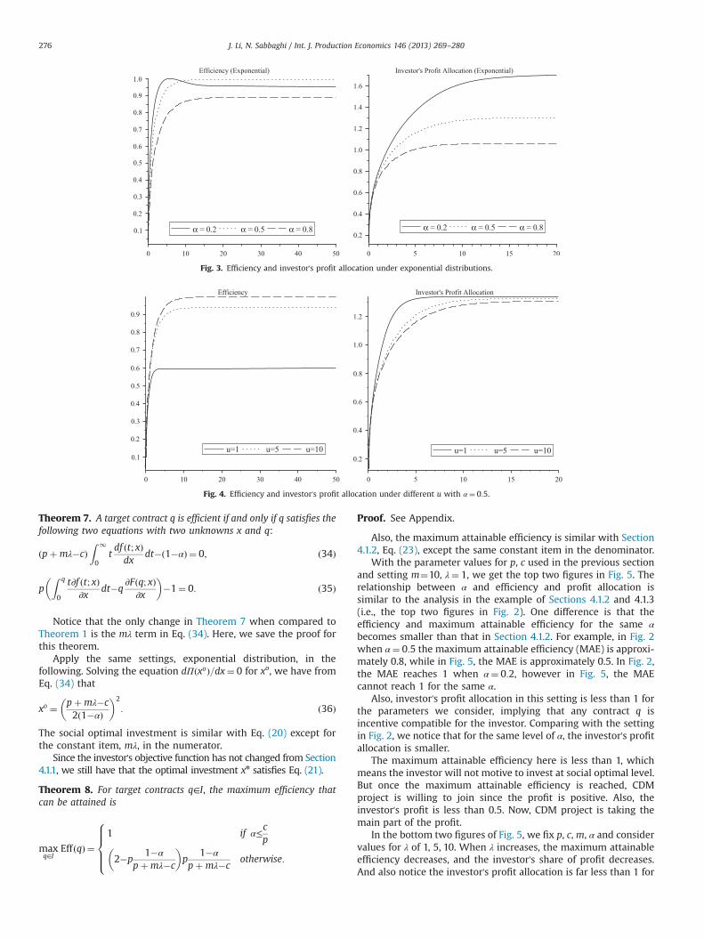
As in the previous section, we consider the parameters p¼12,c¼3 and u¼10 and in Fig. 3 obtain the efficiency and investor'sprofit allocation under demand uncertainty. We observe thatwhen α decreases, the maximum attainable efficiency increases.And when α is very small, e.g., 0.2 in the figure, the maximumefficiency reaches the largest possible value of 1. Again, there issome critical threshold for q in efficiency beyond which the size ofthe contract is not affect investor's efficiency.

Investor's profit allocation also has similar relationship with αas in the previous section, i.e., as α increases, the investor's profitshare decreases. Also, the profit allocation which is greater thanone, negative CDM project's profit, is not considered. There iscritical threshold for q in profit allocation beyond which it is notincentive compatible for the CDM project.

As q goes to infinity, xn reduces to x, and the maximumattainable efficiency (MAE) is

Πðminðx; xoÞÞΠðxoÞ ¼

puffiffiffix

p

uþffiffiffix

p �cffiffiffix

p� 1�αð Þx

puffiffiffiffiffixo

p

uþffiffiffiffiffixo

p �cffiffiffiffiffixo

p� 1�αð Þxo

while the investor's allocation (MAE-I) simplifies to

πiðminðx; xoÞÞΠðminðx; xoÞÞ ¼

p1

1ffiffiffix

p þ 1u

0BB@

1CCA�x

puffiffiffix

p

uþffiffiffix

p �cffiffiffix

p� 1�αð Þx

:

Table 2 shows the numerical examples for the previous analysisabout maximum efficiency and profit allocation for different pairof coefficients.

Similar to Table 1, we see that variables p, c have a relativelysmall effect on the maximum attainable efficiency and a largeeffect on the profit allocation. Variable α affects both maximumattainable efficiency and profit allocation. Also, we observe that forthe same parameter settings, the maximum attainable efficiency isgreater compared with Table 1.

Fig. 2. Efficiency and investor's profit allocation among different distributions.

J. Li, N. Sabbaghi / Int. J. Production Economics 146 (2013) 269–280 275

In addition, it is relatively more difficult for CDM project to beincentivized to agree to the investor once the investor facesdemand uncertainty. This can be observed in our numericalexample in Table 2 since the profit allocation is less than 1 onlyunder two settings (there are five in Table 1) when α is higher andthe margin p�c is greater. Although the requirements for CDMproject to agree to the investor are the same with Section 4.1.1,large margin and fraction of technology value retention, investornow takes the larger fraction of the profit.

After fixing non-market variables (p, c, α), we find the effect ofthe market demand u on efficiency and profit allocation in Fig. 4.For a fixed contract q, a higher u results in a higher maximum

efficiency, which means higher expectation for market demand wouldimprove efficiency. In the same figure, considering only the contracts qfor which the investor's profit allocation is less than 1, for a fixedcontract q, a higher u also results in a lower profit share for theinvestor. Therefore, a larger expected demand has the benefit ofimproved efficiency but results in less of a profit share for the investor.

4.3. Projects with underlying products and without demanduncertainty for CERs

Theorem 7 describes the targets contracts q that motivate theinvestor to invest the system optimal amount under model 3.3.

Fig. 4. Efficiency and investor's profit allocation under different u with α¼ 0:5.

Fig. 3. Efficiency and investor's profit allocation under exponential distributions.

J. Li, N. Sabbaghi / Int. J. Production Economics 146 (2013) 269–280276

Theorem 7. A target contract q is efficient if and only if q satisfies thefollowing two equations with two unknowns x and q:

pþmλ�cð ÞZ 1

0tdf ðt; xÞdx

dt� 1�αð Þ ¼ 0; ð34Þ

pZ q

0

t∂f ðt; xÞ∂x

dt�q∂Fðq; xÞ

∂x

� ��1¼ 0: ð35Þ

Notice that the only change in Theorem 7 when compared toTheorem 1 is the mλ term in Eq. (34). Here, we save the proof forthis theorem.

Apply the same settings, exponential distribution, in thefollowing. Solving the equation dΠðxoÞ=dx¼ 0 for xo, we have fromEq. (34) that

xo ¼ pþmλ�c2ð1�αÞ

� �2

: ð36Þ

The social optimal investment is similar with Eq. (20) except forthe constant item, mλ, in the numerator.

Since the investor's objective function has not changed from Section4.1.1, we still have that the optimal investment xn satisfies Eq. (21).

Theorem 8. For target contracts q∈I, the maximum efficiency thatcan be attained is

maxq∈I

Eff qð Þ ¼1 if α≤

cp

2�p1�α

pþmλ�c

� �p

1�α

pþmλ�cotherwise:

8>>><>>>:

Proof. See Appendix.

Also, the maximum attainable efficiency is similar with Section4.1.2, Eq. (23), except the same constant item in the denominator.

With the parameter values for p, c used in the previous sectionand setting m¼10, λ¼ 1, we get the top two figures in Fig. 5. Therelationship between α and efficiency and profit allocation issimilar to the analysis in the example of Sections 4.1.2 and 4.1.3(i.e., the top two figures in Fig. 2). One difference is that theefficiency and maximum attainable efficiency for the same αbecomes smaller than that in Section 4.1.2. For example, in Fig. 2when α¼ 0:5 the maximum attainable efficiency (MAE) is approxi-mately 0.8, while in Fig. 5, the MAE is approximately 0.5. In Fig. 2,the MAE reaches 1 when α¼ 0:2, however in Fig. 5, the MAEcannot reach 1 for the same α.

Also, investor's profit allocation in this setting is less than 1 forthe parameters we consider, implying that any contract q isincentive compatible for the investor. Comparing with the settingin Fig. 2, we notice that for the same level of α, the investor's profitallocation is smaller.

The maximum attainable efficiency here is less than 1, whichmeans the investor will not motive to invest at social optimal level.But once the maximum attainable efficiency is reached, CDMproject is willing to join since the profit is positive. Also, theinvestor's profit is less than 0.5. Now, CDM project is taking themain part of the profit.

In the bottom two figures of Fig. 5, we fix p, c,m, α and considervalues for λ of 1, 5, 10. When λ increases, the maximum attainableefficiency decreases, and the investor's share of profit decreases.And also notice the investor's profit allocation is far less than 1 for

Fig. 5. Efficiency and investor's profit allocation among different settings.

Fig. 6. Efficiency and investor's profit allocation with/without underlying production.

J. Li, N. Sabbaghi / Int. J. Production Economics 146 (2013) 269–280 277

these values of λ. Since m and λ have a similar effect on theobjective functions, increasing m will have the same effect.In other words, the larger the underlying output or the largerthe underlying profit margin, the lower the maximum attainableefficiency and the lower the investor's profit share (which is betterfor the CDM project).

In Fig. 6, we check the difference in results with the setting inSection 4.1.1 once add an underlying product. The values of p, c, m,λ and α are 12, 3, 10, 1, 0.5, respectively. From the figure, weobserve that the underlying production results in a lower

maximum attainable efficiency, and shift the profits allocationaway from investor to the CDM project. Therefore, an underlyingproduct benefits the CDM project.

4.4. Projects with underlying products and with demand uncertaintyfor CERs

The following theorem, parallels Theorem 5, however we alsohave underlying products produced.

J. Li, N. Sabbaghi / Int. J. Production Economics 146 (2013) 269–280278

Theorem 9. A target contract q is efficient if and only if q satisfies thefollowing two equations with two unknowns x and q:

pZ 1

0t � 1�FD tð Þð Þ � ∂f ðt; xÞ

∂x�f t; xð Þf D tð Þ

� �dt þ mλ�cð Þ

Z 1

0tdf ðt; xÞdx

dt� 1�αð Þ ¼ 0;

ð37Þ

pZ q

0t � 1�FD tð Þð Þ � ∂f ðt; xÞ

∂x�f t; xð Þf D tð Þ

� �dt�q

∂Fðq; xÞ∂x

1�FD qð Þð Þ� �

�1¼ 0: ð38Þ

The proof is the same with proof of Theorem 5 after replacecoefficient -c with mλ-c in Eq. (30).

Follow the same settings, exponential distribution, in Section4.2. Solving the equation dΠðxoÞ=dx¼ 0 for xo, the followingequation implicitly defines xo:

p2

u2ffiffiffiffiffixo

pðuþ

ffiffiffiffiffixo

pÞ2

þmλ�c2ffiffiffiffiffixo

p � 1�αð Þ ¼ 0

Furthermore, for any target contract q, the investor's optimalinvestment xnðqÞ satisfies Eq. (32).

Theorem 10. Suppose the value xo, x are defined implicitly by theequations

pu2

uþffiffiffiffiffixo

p� �2 þ mλ�cð Þ�2 1�αð Þffiffiffiffiffixo

p¼ 0

12

p

xffiffiffix

p 1x

þ 1u

� ��1¼ 0:

we have that for contracts q∈I, the maximum efficiency that can beattained is

maxq∈I

Eff qð Þ ¼ΠðxÞΠðxoÞ if x≤xo

1 otherwise:

8<:

Proof. See Appendix.

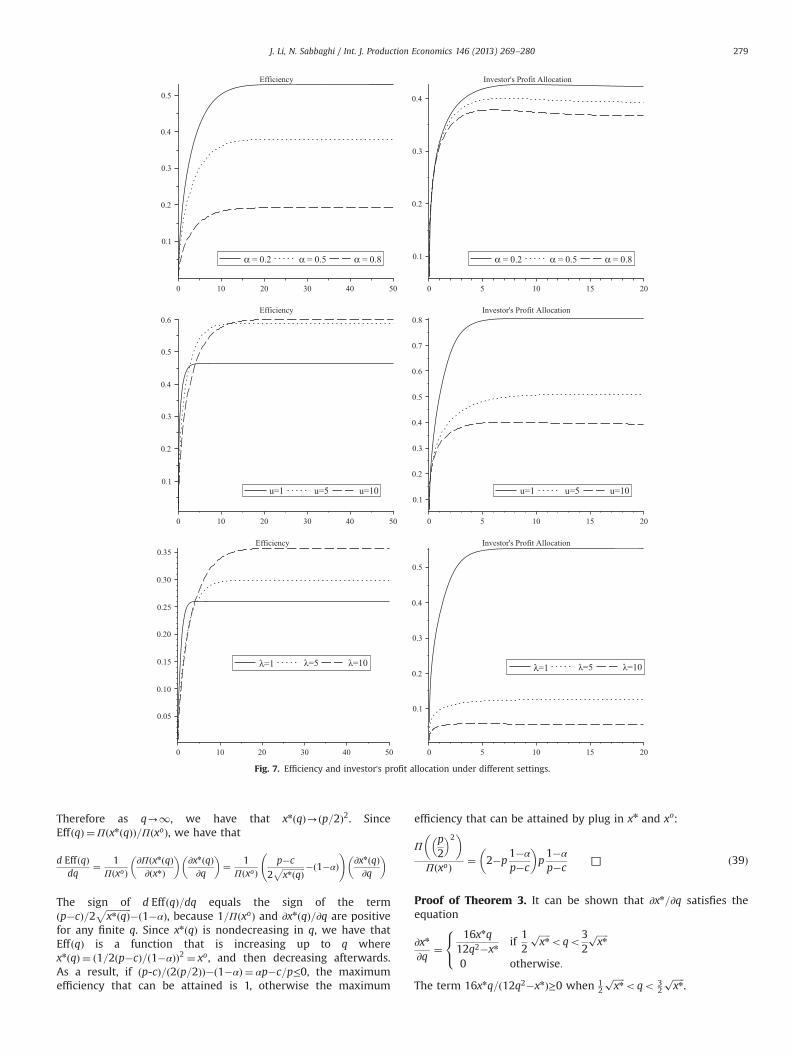
The top two figures in Fig. 7 show the efficiency and investor'sprofit allocation as defined in Eqs. (16) and (17) with parametersp¼12, c¼3, m¼10, λ¼ 1 and u¼10. When α increases, bothefficiency and investor's profit allocation decrease, same as thetrends in Section 4.2 (Fig. 3) for the same parameters. However, themaximum attainable efficiency is lower for each α when comparingwith Section 4.2. And for each α, the investor's profit allocation islower too. Also, the investor's profit allocation is less than 1 demon-strating the CDM project is incentive compatible for the investorand furthermore, it is less than 0.5 so that the CDM project's profitis larger than the investor's profit. Therefore, with underlyingproducts, both the CDM project and investor are motivated toparticipate, even though the investor faces demand uncertainty.

The middle two figures show the relationships of expecteddemand u with efficiency and investor's profit allocation (α¼ 0:5).These relationships are similar with those in Fig. 4, where therewas no underlying product. In particular, for a higher expectedmarket demand, the investor will take less profit share and thecontract attains higher efficiency.

The bottom two figures show the underlying production'seffect. The relationship we observe is similar to the middle twofigures. A higher output of underlying product (or a higher profitmargin for underlying product) will improve contract efficiencyand the CDM project's profit allocation increases.

Also, from the figures we observe, that there is a critical valuefor q beyond which the profits and thus efficiency remains thesame. Thus, the size of contract would no longer have an effectbeyond that critical value. From the analysis, this follows because

as q becomes larger, xnðqÞ reaches a limit, i.e., x, and all of theprofits depend only on q and x.

5. Conclusions

We consider two broad categories of CDM projects, those thathave an underlying product generated in addition to the CERcredits and those projects that do not. Within each category, weconsider CDM projects that have demand uncertainty for the CERcredits generated and those that do not. For these CDM projects,we consider two firms, a project and a potential investor, and findthe optimal investment decision for an investor faced with a targetcontract for CER credits from the project. We also find the optimalinvestment decision for the overall system, thinking of theinvestor and project being one single firm. Then, we analyze theefficiency of the target contract and explore the allocation of profitbetween the firms.

We find that it is not always possible for target contracts toinduce the investor to invest the system optimal amount. How-ever, we find the maximum efficiency that can be attained bychoosing the appropriate target contract. Furthermore, when theresidual value of the technology investment is small, the investorcan attain a higher efficiency and a higher percentage of thesystem profits. Although the categories of CDM projects that weconsider are different, we find that the maximum attainableefficiency is a function of a ratio of the fixed cost (technologyvalue lost) to the gross margin. In addition, for all the settings weconsider, when the residual value remaining for the technology issmall enough target contracts are desirable in that they can attainthe maximum possible efficiency. Furthermore, when there is ademand uncertainty, a higher expected market demand results inthe investor taking less profit share and the contract attaininghigher efficiency. And when there is an underlying product, ahigher output (or a higher profit margin for underlying product)will improve contract efficiency and increase the CDM project'sprofit allocation.

Appendix A

Proof for Theorem 1. Under our assumptions, any realization ofthe random function Q(x) is concave in x, therefore we have thatthe realization of the random function minðq;Q ðxÞÞ is concave in x.As a result, the investor's profit πiðq; xÞ ¼ pE½minðq;Q ðxÞÞ��x isalso concave in x. Furthermore, observe that the system's profitΠðxÞ ¼ ðp�cÞE½Q ðxÞ��ð1�αÞx is also concave in x. Therefore, it isboth necessary and sufficient that at the system optimal invest-ment xo the equation dΠðxoÞ=dx¼ 0 holds and that at the investoroptimal investment xn the equation ∂πiðq; xnÞ=∂x¼ 0 holds for anychoice of q. Therefore, we have that xnðqÞ ¼ xo if and only if there isan investment amount x and target contract q that satisfies theequations dΠðxÞ=dx¼ 0 and ∂πiðq; xÞ=∂x¼ 0 resulting in Eqs. (18)and (19), respectively. □

Proof for Theorem 2. It can be shown that dxn=dq satisfies theequation

dxn

dq¼

2e�q=ffiffiffiffixn

p qffiffiffiffiffixn

p p

2þ e�q=ffiffiffiffixn

p qffiffiffix

p� �2 pffiffiffi

xp

We have that dxn=dq40, when xnðqÞ40. The investor's first ordercondition (Eq. (19)) can be reexpressed as

p �12

� 1ffiffiffix

p þ e�q=ffiffix

p 1ffiffiffix

p þ e�q=ffiffix

p� q � 1

x

� �� �¼ 1

Fig. 7. Efficiency and investor's profit allocation under different settings.

J. Li, N. Sabbaghi / Int. J. Production Economics 146 (2013) 269–280 279

Therefore as q-1, we have that xnðqÞ-ðp=2Þ2. SinceEffðqÞ ¼ΠðxnðqÞÞ=ΠðxoÞ, we have that

d EffðqÞdq

¼ 1ΠðxoÞ

∂ΠðxnðqÞ∂ðxnÞ

� �∂xnðqÞ∂q

� �¼ 1

ΠðxoÞp�c

2ffiffiffiffiffiffiffiffiffiffiffixnðqÞ

p � 1�αð Þ !

∂xnðqÞ∂q

� �

The sign of d Eff ðqÞ=dq equals the sign of the termðp�cÞ=2

ffiffiffiffiffiffiffiffiffiffiffixnðqÞ

p�ð1�αÞ, because 1=ΠðxoÞ and ∂xnðqÞ=∂q are positive

for any finite q. Since xnðqÞ is nondecreasing in q, we have thatEffðqÞ is a function that is increasing up to q wherexnðqÞ ¼ ð1=2ðp�cÞ=ð1�αÞÞ2 ¼ xo, and then decreasing afterwards.As a result, if ðp-cÞ=ð2ðp=2ÞÞ�ð1�αÞ ¼ αp�c=p≤0, the maximumefficiency that can be attained is 1, otherwise the maximum

efficiency that can be attained by plug in xn and xo:

Πp2

� �2� �ΠðxoÞ ¼ 2�p

1�α

p�c

� �p1�α

p�c□ ð39Þ

Proof of Theorem 3. It can be shown that ∂xn=∂q satisfies theequation

∂xn

∂q¼

16xnq12q2�xn

if12

ffiffiffiffiffixn

poqo3

2ffiffiffiffiffixn

p

0 otherwise:

8<:

The term 16xnq=ð12q2�xnÞ≥0 when 12

ffiffiffiffiffixn

poqo 3

2

ffiffiffiffiffixn

p.

J. Li, N. Sabbaghi / Int. J. Production Economics 146 (2013) 269–280280

From Eqs. (27) and (28) we have that as q-1, xnðqÞ-ðp=2Þ2.Since EffðqÞ ¼ΠðxnðqÞÞ=ΠðxoÞ, we have that

d Eff ðqÞdq

¼ 1ΠðxoÞ

∂ΠðxnðqÞ∂ðxnÞ

� �∂xnðqÞ∂q

� �¼ 1

ΠðxoÞp�c

2ffiffiffiffiffiffiffiffiffiffiffixnðqÞ

p � 1�αð Þ !

∂xnðqÞ∂q

� �

When 12

ffiffiffiffiffixn

poqo 3

2

ffiffiffiffiffixn

p, the sign of d Eff ðqÞ=dq equals the sign of

the term ðp�cÞ=2ffiffiffiffiffiffiffiffiffiffiffixnðqÞ

p�ð1�αÞ, because 1=ΠðxoÞ and ∂xnðqÞ=∂q are

positive for any finite q. Since xnðqÞ is nondecreasing in q, we havethat EffðqÞ is a function that is increasing up to q wherexnðqÞ ¼ ð1=2ðp�cÞ=ð1�αÞÞ2 ¼ xo, and then decreasing afterwards.As a result, if ðp-cÞ=ð2ðp=2ÞÞ�ð1�αÞ ¼ ðαp�cÞ=p≤0, the maximumefficiency that can be attained is 1, otherwise the maximumefficiency that can be attained is

Πp2

� �2� �ΠðxoÞ ¼ 2�p

1�α

p�c

� �p1�α

p�c□

Proof of Theorem 4. It can be shown that dxn=dq≥0 and further-more, as q-1, it can be shown that xnðqÞ-ðpθ=2Þ2. SinceEffðqÞ ¼ΠðxnðqÞÞ=ΠðxoÞ, we have that

d Eff ðqÞdq

¼ 1ΠðxoÞ

∂ΠðxnðqÞ∂ðxnÞ

� �∂xnðqÞ∂q

� �¼ 1

ΠðxoÞðp�cÞθ2

ffiffiffiffiffiffiffiffiffiffiffixnðqÞ

p � 1�αð Þ !

∂xnðqÞ∂q

� �

The sign of d Eff ðqÞ=dq equals the sign of the termðp�cÞθ=2

ffiffiffiffiffiffiffiffiffiffiffixnðqÞ

p�ð1�αÞ, because 1=ΠðxoÞ and ∂xnðqÞ=∂q are positive

for any finite q. Since xnðqÞ is nondecreasing in q, we havethat EffðqÞ is a function that is increasing up to q wherexnðqÞ ¼ ðθðp-cÞ=ð2ð1�αÞÞÞ2 ¼ xo, and then decreasing afterwards.As a result, if ðp-cÞθ=ð2ðp=2ÞθÞ�ð1�αÞ ¼ ðαp�cÞ=p≤0, the maximumefficiency that can be attained is 1, otherwise the maximumefficiency that can be attained is

Π

p2

� �θ

� �2�

ΠðxoÞ ¼ 2�p1�α

p�c

� �p1�α

p�c: □

Proof of Theorem 5. Under our assumptions, any realization ofthe random function Q(x) is concave in x, therefore we have thatthe realization of the random function minðq;Q ðxÞ;DÞ is concave inx. As a result, the investor's profit πiðq; xÞ ¼ pE½minðq;Q ðxÞ;DÞ��x isalso concave in x. Furthermore, observe that the system's profitΠðxÞ ¼ ðp�cÞE½minðQ ðxÞ;DÞ��ð1�αÞx is also concave in x. Therefore,it is both necessary and sufficient that at the system optimalinvestment xo the equation dΠðxoÞ=dx¼ 0 holds and that at theinvestor optimal investment xn the equation ∂πiðq; xnÞ=∂x¼ 0 holdsfor any choice of q. As a result, we have that xnðqÞ ¼ xo if and only ifthere is an investment amount x and target contract q that satisfiesthe equations dΠðxÞ=dx¼ 0 and ∂πiðq; xÞ=∂x¼ 0 resulting in Eqs.(18) and (19), respectively. □

Proof of Theorem 6. It can be shown that ΠðxÞ is concave in x andis increasing up to xo and decreasing for all values that are largerthan xo. Furthermore the following equation implicitly defines theinvestor's investment level xnðqÞ:

�12

p �1þ e�ð1=ffiffiffiffixn

pþ1=uÞq þ qe�ð1=

ffiffiffiffixn

pþ1=uÞq 1ffiffiffiffiffi

xnp þ 1

u

� �� �

x3=21ffiffiffiffiffixn

p þ 1u

� � �1¼ 0: ð40Þ

From Eq. (32), we observe that xnðqÞ is increasing in q and it can beshown that as q tends to infinity, we have that xnðqÞ equals thesolution x that satisfies Eq. (33). As a result, if x4xo, we have that themaximum attainable efficiency is 1, otherwise it is ΠðxÞ=ΠðxoÞ. □

Proof of Theorem 8. Since the investor's objective function is thesame as in Section 4.1.1, we have that dxn=dq≥0 and as q-1, wehave that xnðqÞ-ðp=2Þ2. Since EffðqÞ ¼ΠðxnðqÞÞ=ΠðxoÞ, we have that

d Eff ðqÞdq

¼ 1ΠðxoÞ

∂ΠðxnðqÞ∂ðxnÞ

� �∂xnðqÞ∂q

� �¼ 1

ΠðxoÞpþmλ�c

2ffiffiffiffiffiffiffiffiffiffiffixnðqÞ

p � 1�αð Þ !

∂xnðqÞ∂q

� �

The sign of d EffðqÞ=dq equals the sign of the term ðpþmλ�cÞ=2

ffiffiffiffiffiffiffiffiffiffiffixnðqÞ

p�ð1�αÞ, because 1=ΠðxoÞ and ∂xnðqÞ=∂q are positive for any

finite q. Since xnðqÞ is nondecreasing in q, we have that EffðqÞ is afunction that is increasing up to q where xn qð Þ ¼ ð12 p�cð Þ= 1�αð ÞÞ2,and then decreasing afterwards. As a result, if ðp�cÞ=ð2ðp=2ÞÞ�ð1�αÞ ¼ ðαp�cÞ=p≤0, the maximum efficiency that can be attainedis 1, otherwise the maximum efficiency that can be attained is

Πp2

� �2� �ΠðxoÞ ¼ 2�p

1�α

pþmλ�c

� �p

1�α

pþmλ�c□

Proof of Theorem 10. The proof is similar to the proof of Theorem6 since the investor has the same objective function in bothsettings and the total profit still is concave in the investment levelx. As a result, if x≥xo then the maximum attainable efficiency is 1,otherwise it is ΠðxÞ=ΠðxoÞ. □

References

Alexandre Kossoy, Guigon Pierre. 2012. State and Trends of the Carbon Market2012. World Bank.

Azad, A.K., 2012. Statistical weibull's distribution analysis for wind power of thetwo dimensional ridge areas. International Journal of Advanced RenewableEnergy Research 1, 8–13.

Benjamin, C. Esty, Megginson, William L., 2003. Creditor's rights enforcement anddebt ownership structure: evidence from the global syndicated loans market.Journal of Financial and Quantitative Analysis 38, 37–60.

Berkovitch, Elazar, HanKim, E., 1990. Financial contracting and leverage inducedover- and under- investments incentives. The Journal of Finance 45, 765–794.

Brealey, Richard A., Cooper, Ian A., Habib, Michel A., 1996. Using project finance tofund infrastructure investments. Journal of Applied Corporate Finance 9, 25–39.

Esty, Benjamin C., 2002. Returns on project-financed investments: evolution andmanagerial implications. Journal of Applied Corporate Finance 15, 71–86.

Esty, Benjamin C., 2003. The economic motivations for using project finance.Working Paper. Harvard Business School, Boston.

Esty, Benjamin C., 2007. An overview of project finance and infrastructure finance-2006 update. Case study 9-207-107. Harvard Business School, Boston.

Flannery, Mark J., Venkataraman, Subramanyam, Houston, Joel F., 1993. Financingmultiple investment projects. Financial Management 22, 161–172.

Francesco, Corielli, Steffanoni, Alessandro, Gatti, Stefano, 2010. Risk shiftingthrough nonfinancial contracts: effects on loan spreads and capital structureof project finance deals. Journal of Money, Credit and Banking 42, 1295–1320.

Jensen, Michael C., Meckling, William H., 1976. Theory of the firm: managerial behavior,agency costs, and ownership structure. Journal of Financial Economics 3, 305–360.

John, Teresa A., John, Kose, 1991. Optimality of project financing: theory andempirical implications in finance and accounting. Review of QuantitativeFinance and Accounting 1, 51–74.

Johnson, Norman L., Balakrishnan, N., Kotz, Samuel, 1994. Continuous UnivariateDistributions, vol. 12. Wiley Interscience.

Marco, Sorge, Gadanecz, Blaise, 2008. The term structure of credit spreads inproject finance. International Journal of Finance and Economics 13, 68–81.

Shah, Salman, Thakor, Anjan V., 1987. Optimal capital structure and projectfinancing. Journal of Economics Theory 42, 209–243.

The Royal Academy of Engineering, RWE NPOWER. n.d. Wind turbine powercalculations.

UNEP, 2004. Legal Issues Guidebook to the Clean Development Mechanism.UNEP, EcoSecurities, 2007. Guidebook to Financing CDM Projects.