Decision Making in Robotsand Autonomous Agents

Learning in Repeated Interactions

Stefano V. Albrecht

School of Informatics

27 February 2015

Learning in Repeated Interactions

I How can agent learn to interact with other agents?

I What kind of behaviour do we want to learn?

I Learn individually or together?

I Many different methods...

I In this lecture: reinforcement learning

Recap

Markov Decision Process:

I states S , actions A

I stochastic transition P(s ′|s, a)

I utility/reward u(s, a) (can be random variable)

Reinforcement Learning:

I “reinforce” good actions

I learn optimal action policy π∗

I e.g. value iteration, policy iteration, ...

→ require knowledge of model, e.g. P/u

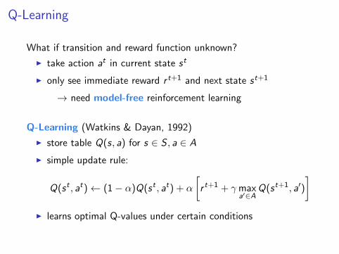
Q-Learning

What if transition and reward function unknown?

I take action at in current state st

I only see immediate reward r t+1 and next state st+1

→ need model-free reinforcement learning

Q-Learning (Watkins & Dayan, 1992)

I store table Q(s, a) for s ∈ S , a ∈ A

I simple update rule:

Q(st , at)← (1− α)Q(st , at) + α

[r t+1 + γmax

a′∈AQ(st+1, a′)

]

I learns optimal Q-values under certain conditions

Q-Learning in Stochastic Games

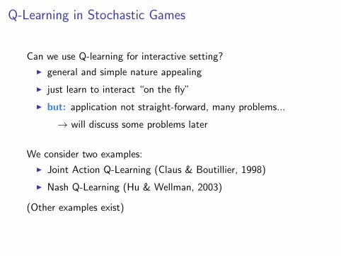
Can we use Q-learning for interactive setting?

I general and simple nature appealing

I just learn to interact “on the fly”

I but: application not straight-forward, many problems...

→ will discuss some problems later

We consider two examples:

I Joint Action Q-Learning (Claus & Boutillier, 1998)

I Nash Q-Learning (Hu & Wellman, 2003)

(Other examples exist)

Joint Action Q-Learning (JAL) (Claus & Boutillier, 1998)

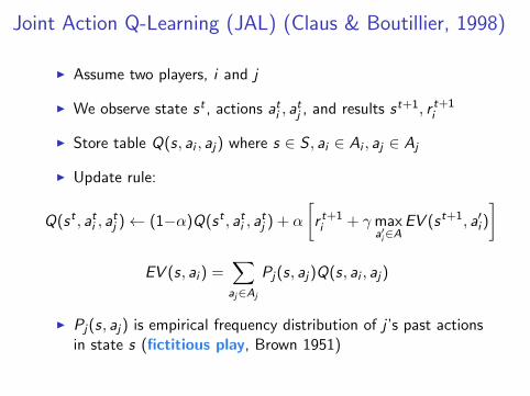
I Assume two players, i and j

I We observe state st , actions ati , atj , and results st+1, r t+1

i

I Store table Q(s, ai , aj) where s ∈ S , ai ∈ Ai , aj ∈ Aj

I Update rule:

Q(st , ati , atj )← (1−α)Q(st , ati , a

tj ) + α

[r t+1i + γmax

a′i∈AEV (st+1, a′i )

]

EV (s, ai ) =∑

aj∈Aj

Pj(s, aj)Q(s, ai , aj)

I Pj(s, aj) is empirical frequency distribution of j ’s past actionsin state s (fictitious play, Brown 1951)

JAL and Nash Equilibrium

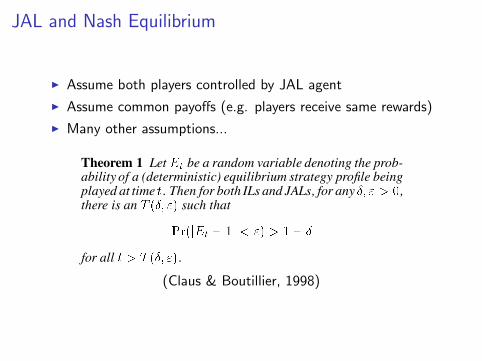
I Assume both players controlled by JAL agent

I Assume common payoffs (e.g. players receive same rewards)

I Many other assumptions...

0

0.2

0.4

0.6

0.8

1

0 500 1000 1500 2000 2500

Prob

. of a

ctio

ns

Number of Interactions

Strategy of agent A

Prob. of a0Prob. of a1Prob. of a2

Figure 3: ’s strategy in climbing game

0

0.2

0.4

0.6

0.8

1

0 500 1000 1500 2000 2500

Prob

. of a

ctio

ns

Number of Interactions

Strategy of agent B

Prob. of b0Prob. of b1Prob. of b2

Figure 4: ’s strategy in climbing game

Initially, the two learners are almost certainly going to beginto play the nonequilibrium strategy profile . This isseen clearly in Figures 3, 4 and 5. However, once they “set-tle” at this point, as long as exploration continues, agentwill soon find to be more attractive—so long as contin-ues to primarily choose . Once the nonequilibrium point

is attained, agent tracks ’s move and begins toperform action . Once this equilibrium is reached, theagents remain there.This phenomenon will obtain in general, allowing one to

conclude that the multiagent Q-learning schemes we haveproposed will converge to equilibria almost surely. The con-ditions that are required in both cases are:

The learning rate decreases over time such thatand .

Each agent samples each of its actions infinitely often.

Parameter settings for these figures: initial temperature 10000is decayed at rate .

0

0.2

0.4

0.6

0.8

1

0 500 1000 1500 2000 2500

perfo

rmed

join

t act

ions

(per

)

Number of Interactions

Joint actions

joint action a0b0joint action a0b1joint action a0b2joint action a1b0joint action a1b1joint action a1b2joint action a2b0joint action a2b1joint action a2b2

Figure 5: Joint actions in climbing game

The probability of agent choosing action isnonzero.

Each agent’s exploration strategy is exploitive. That is,, where is a random variable de-

noting the event that some nonoptimal action was takenbased on ’s estimated values at time .

The first two conditions are required of Q-learning, and thethird, if implemented appropriately (e.g., with appropriatelydecayed temperature), will ensure the second. Furthermore,it ensures that agents cannot adopt deterministic explorationstrategies and become strictly correlated. Finally, the lastcondition ensures that agents exploit their knowledge. In thecontext of ficticious play and its variants, this explorationstrategy would be asymptotically myopic [5]. This is nec-essary to ensure that an equilibrium will be reached. Underthese conditions we have:Theorem 1 Let be a random variable denoting the prob-ability of a (deterministic) equilibrium strategy profile beingplayed at time . Then for both ILs and JALs, for any ,there is an such that

for all .Intuitively (and somewhat informally), the dynamics of

the learning process behaves as follows. If the agents are inequilibrium, there is a nonzero probability of moving out ofequilibrium; but this generally requires a (rather dense) se-ries of exploratorymoves by one or more agents. The proba-bility of this occurring decreases over time, making the like-lihood of leaving an equilibrium just obtained vanish overtime (both for JALs and ILs). If at some point the agents’estimated Q-values are such that a nonequilibrium is mostlikely, the likelihood of this state of affairs remaining alsovanishes over time. As an example, consider the climbinggame above. Once agents begin to play regularly,agent is still required to explore. After a sufficient sam-pling of action —without agent simultaneously explor-ing and moving away from — will look more attractivethan and this best replywill be adopted. Decreasing explo-ration ensures that the odds of simultaneous exploration de-

(Claus & Boutillier, 1998)

Nash Q-Learning (NashQ) (Hu & Wellman, 2003)

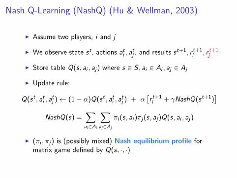
I Assume two players, i and j

I We observe state st , actions ati , atj , and results st+1, r t+1

i , r t+1j

I Store table Q(s, ai , aj) where s ∈ S , ai ∈ Ai , aj ∈ Aj

I Update rule:

Q(st , ati , atj )← (1− α)Q(st , ati , a

tj ) + α

[r t+1i + γNashQ(st+1)

]

NashQ(s) =∑

ai∈Ai

∑

aj∈Aj

πi (s, ai )πj(s, aj)Q(s, ai , aj)

I (πi , πj) is (possibly mixed) Nash equilibrium profile formatrix game defined by Q(s, ·, ·)

NashQ and Nash Equilibrium

I Assume both players controlled by NashQ agent

I Assume several other restrictions ... including:HU AND WELLMAN

Assumption 3 One of the following conditions holds during learning.3Condition A. Every stage game (Q1t (s), . . . ,Qn

t (s)), for all t and s, has a global optimal point,and agents’ payoffs in this equilibrium are used to update their Q-functions.Condition B. Every stage game (Q1t (s), . . . ,Qn

t (s)), for all t and s, has a saddle point, andagents’ payoffs in this equilibrium are used to update their Q-functions.

We further define the distance between two Q-functions.

Definition 15 For Q, Q 2Q, define

k Q� Q k ⌘ maxjmaxsk Qj(s)� Q j(s) k( j,s)

⌘ maxjmaxsmaxa1,...,an

|Qj(s,a1, . . . ,an)� Q j(s,a1, . . . ,an)|.

Given Assumption 3, we can establish that Pt is a contraction mapping operator.

Lemma 16 k PtQ�PtQ k β k Q� Q k for all Q, Q 2Q.

Proof.

k PtQ�PtQ k = maxjk PtQj�PtQ j k( j)

= maxjmaxs

| βπ1(s) · · ·πn(s)Qj(s)�βπ1(s) · · · πn(s)Q j(s) |

= maxjβ | π1(s) · · ·πn(s)Qj(s)� π1(s) · · · πn(s)Q j(s) |

We proceed to prove that

|π1(s) · · ·πn(s)Qj(s)� π1(s) · · · πn(s)Q j(s)|k Qj(s)� Q j(s) k .

To simplify notation, we use σ j to represent π j(s), and σ j to represent π j(s). The proposition wewant to prove is

|σ jσ� jQ j(s)� σ jσ� jQ j(s)|k Qj(s)� Q j(s) k .

Case 1: Suppose both (σ1, . . . ,σn) and (σ1, . . . , σn) satisfy Condition A in Assumption 3, whichmeans they are global optimal points.

If σ jσ� jQ j(s)� σ jσ� jQ j(s), we have

σ jσ� jQ j(s)� σ jσ� jQ j(s) σ jσ� jQ j(s)�σ jσ� jQ j(s)= ∑

a1,...,anσ1(a1) · · ·σn(an)

�Qj(s,a1, . . . ,an)� Q j(s,a1, . . . ,an)

�

∑a1,...,an

σ1(a1) · · ·σn(an) k Qj(s)� Q j(s) k (15)

= k Qj(s)� Q j(s) k,3. In our statement of this assumption in previous writings (Hu and Wellman, 1998, Hu, 1999), we neglected to includethe qualification that the same condition be satisfied by all stage games. We have made the qualification more explicitsubsequently (Hu and Wellman, 2000). As Bowling (2000) has observed, the distinction is essential.

1050

(Hu & Wellman, 2003)

I Then the learning converges to a Nash equilibrium

Assumptions in Learning Methods

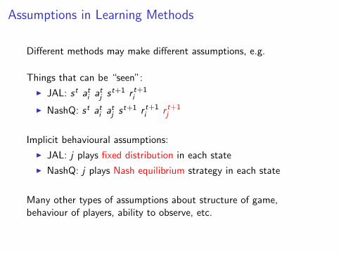
Different methods may make different assumptions, e.g.

Things that can be “seen”:

I JAL: st ati atj st+1 r t+1i

I NashQ: st ati atj st+1 r t+1i r t+1

j

Implicit behavioural assumptions:

I JAL: j plays fixed distribution in each state

I NashQ: j plays Nash equilibrium strategy in each state

Many other types of assumptions about structure of game,behaviour of players, ability to observe, etc.

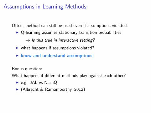
Assumptions in Learning Methods

Often, method can still be used even if assumptions violated:

I Q-learning assumes stationary transition probabilities

→ Is this true in interactive setting?

I what happens if assumptions violated?

I know and understand assumptions!

Bonus question:

What happens if different methods play against each other?

I e.g. JAL vs NashQ

I (Albrecht & Ramamoorthy, 2012)

Excursion:

Ad Hoc Coordination in Multiagent Systems

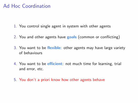
Ad Hoc Coordination

1. You control single agent in system with other agents

2. You and other agents have goals (common or conflicting)

3. You want to be flexible: other agents may have large varietyof behaviours

4. You want to be efficient: not much time for learning, trialand error, etc.

5. You don’t a priori know how other agents behave

Ad Hoc Coordination

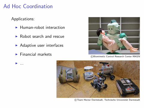
Applications:

I Human-robot interaction

I Robot search and rescue

I Adaptive user interfaces

I Financial markets

I ...

c©Biomimetic Control Research Center RIKEN

c©Team Hector Darmstadt, Technische Universitat Darmstadt

Ad Hoc Coordination

Human-robot interaction:

I Humans can exhibit large variety of behaviours for given task

→ need flexibility!

I Humans expect machines to learn and react quickly

→ need efficiency!

I Machine does not know ahead of time how human behaves

→ no prior coordination of behaviours!

Ad Hoc Coordination

Hard problem:

I Agents may have large variety of behaviours

I Behaviours initially unknown

General learning algorithms not suitable:

I Require long learning periods (e.g. RL)

I Often designed for homogeneous setting

I Many restrictive assumptions (discussed earlier)

Idea

Reduce complexity of problem by assuming that:

1. Agents draw their latent policy from some set

2. Policy assignment governed by unknown distribution

If policy set known:

I Learn distribution, play best-response

If policy set unknown:

I “Guess” policy set, find closest policy, play best-response

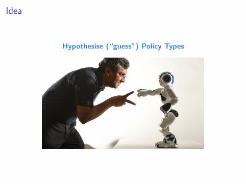
Idea

Hypothesise (“guess”) Policy Types

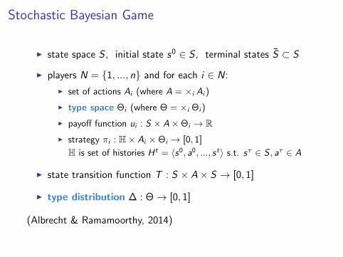
Stochastic Bayesian Game

I state space S , initial state s0 ∈ S , terminal states S ⊂ S

I players N = {1, ..., n} and for each i ∈ N:

I set of actions Ai (where A = ×i Ai )

I type space Θi (where Θ = ×i Θi )

I payoff function ui : S × A×Θi → RI strategy πi : H× Ai ×Θi → [0, 1]

H is set of histories H t = 〈s0, a0, ..., st〉 s.t. sτ ∈ S , aτ ∈ A

I state transition function T : S × A× S → [0, 1]

I type distribution ∆ : Θ→ [0, 1]

(Albrecht & Ramamoorthy, 2014)

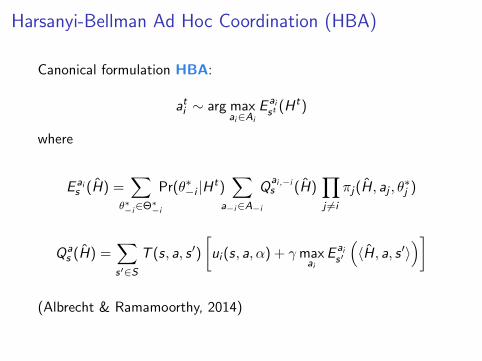
Harsanyi-Bellman Ad Hoc Coordination (HBA)

Canonical formulation HBA:

ati ∼ arg maxai∈Ai

E aist (Ht)

where

E ais (H) =

∑

θ∗−i∈Θ∗−i

Pr(θ∗−i |Ht)∑

a−i∈A−i

Qai,−is (H)

∏

j 6=i

πj(H, aj , θ∗j )

Qas (H) =

∑

s′∈ST (s, a, s ′)

[ui (s, a, α) + γmax

aiE ais′

(〈H, a, s ′〉

)]

(Albrecht & Ramamoorthy, 2014)

References (Reading List)

In order of appearance:

C. Watkins, P. Dayan: Q-Learning. MLJ, 1992

C. Claus, C. Boutilier: The Dynamics of Reinforcement Learning inCooperative Multiagent Systems. AAAI, 1998

J. Hu, M. Wellman: Nash Q-Learning for General-Sum StochasticGames. JMLR, 2003

G. Brown: Iterative Solutions of Games by Fictitious Play. ActivityAnalysis of Production and Allocation, 1951

S. Albrecht, S. Ramamoorthy: Comparative Evaluation of MALAlgorithms in a Diverse Set of Ad Hoc Team Problems. AAMAS, 2012

S. Albrecht, S. Ramamoorthy: On Convergence and Optimality ofBest-Response Learning with Policy Types in Multiagent Systems. UAI,2014