Decision-support tool for assessing future nuclear

reactor generation portfolios.

Shashi Jain ∗ Ferry Roelofs † Cornelis W. Oosterlee ‡

September 9, 2013

Abstract

Capital costs, fuel, operation and maintenance (O&M) costs, and elec-tricity prices play a key role in the economics of nuclear power plants,where especially capital costs are known to be highly uncertain. Differ-ent nuclear reactor types compete economically by having either lowerand less uncertain construction costs, increased efficiencies, lower and lessuncertain fuel cycles and O&M costs etc. The decision making processrelated to nuclear power plants requires a holistic approach that takes intoaccount the key economic factors and their uncertainties. We here presenta decision-support tool, that satisfactorily takes into account the majoruncertainties in the cost elements of a nuclear power plant, to providean optimal portfolio of nuclear reactors. The portfolio so obtained, un-der our model assumptions and the constraints considered, maximizes thecombined returns for a given level of risk or uncertainty. These decisionsare made using a combination of real option theory and mean-varianceportfolio optimization.

1 Introduction

The global electricity demand is expected to double to over 30,000 TWh annu-ally by the year 2030 and meeting this demand without substantially exacer-bating the risks of climate change requires a solution comprised of a variety oftechnologies on both the supply and demand side of the energy system (Pacalaand Socolow (2004), Holdren (2006) and European Commission (2007)). Nu-clear power can play a key role in meeting the projected large absolute increasein energy demand while mitigating the risks of serious climate disruption. Thefact that countries seem keen on building nuclear power stations suggests thattheir relative costs compared to low-carbon alternatives seem attractive to atleast potential investors (Kessides, 2010). However, there are some concernsrelated to uncertainties underlying the various costs elements of nuclear power

∗TU Delft, Delft Institute of Applied Mathematics, Delft, the Netherlands, email:s.jain@cwi.nl, Nuclear Research Group, Petten, and thanks to CWI–Centrum Wiskunde &Informatica, Amsterdam.

†Nuclear Research Group, Petten, email: roelofs@nrg.eu‡CWI–Centrum Wiskunde & Informatica, Amsterdam, the Netherlands, email:

c.w.oosterlee@cwi.nl, and TU Delft, Delft Institute of Applied Mathematics

1

that are reflected in the wide range of cost estimates, cost overruns and sched-ule delays, for example of Finland’s Olkiluoto and France’s Flamanville nuclearpower plants.

There have been numerous studies on the economics of nuclear power in re-cent years which use levelized cost 1 of electricity to compare the economics ofdifferent generation technologies. The levelized cost methodology used in thesestudies however does not address the role of risks and uncertainties involved.Methodologies that take into account the large and diverse set of risks character-izing investment in nuclear power are required. This paper concentrates on theeffect of risks and uncertainties on investment decisions related to the nuclearindustry and the use of diversification to mitigate some of these risks. FollowingRoques et al. (2008) and Fortin et al. (2007) we use a two-step approach, wherefirst real options optimal investment decisions are taken at the plant level, andthen mean-variance portfolio (MVP here after) theory is used to minimize theuncertainties of returns for a portfolio of nuclear reactors.

The seminal literature using MVP techniques in the power sector concen-trated on fuel price risk, and focussed on minimizing generation cost, which,under ideal regulations of a vertically integrated franchise monopoly, shouldmaximise social welfare. Awerbuch and Berger (2003) use MVP to identify theoptimal European energy technology mix, considering not only fuel price riskbut also Operation and Maintenance (O&M), as well as construction periodrisks, while Jansen et al. (2006) use MVP to explore different scenarios of theelectricity system development in the Netherlands. Roques et al. (2008) appliedthe portfolio theory from a private investor perspective to identify optimal port-folios for electricity generators in the UK electricity market, concentrating onprofit risk rather than production costs risk. Fortin et al. (2007) suggest theuse of Conditional Value-at-Risk (CVaR) for portfolio optimization rather thanmean-variance portfolio and provide a detailed review of the literature in thisarea.

Real options analysis (ROA) has been applied to the energy sector planningfor years, since the special features of the electricity sector, such as uncertainty,irreversibility and flexibility to postpone investments, make standard investmentrules solely relying on the net present value (NPV) not advisable as they ignorethe options involved in a sequence of decisions. The real options approach formaking investment decisions in projects with uncertainties was pioneered byArrow and Fisher (1974).Using real options it’s possible to value the option todelay, expand or abandon a project with uncertainties, when such decisions aremade following an optimal policy.

Pindyck (1993) employs real options to analyse the decisions to start, con-tinue or abandon the construction of nuclear power plants. There, uncertaincosts of a reactor rather than expected cash flows are considered for making theoptimal decisions. Rothwell (2006) uses ROA to compute the critical electric-ity price at which a new advanced boiling water reactor should be ordered inTexas. Naito et al. (2010) apply real options theory to determine the optimaltiming for decommissioning of existing nuclear power plants and construction oftheir replacements. Zhu (2012) uses real options to evaluate the Sanmen nuclear

1The levelized cost of a project is equivalent to the constant euro price of electricity thatwould be required over the life of the plant to cover all operating expenses, interest andrepayment obligations on project debt, and taxes plus an acceptable return to equity investorsover the economic life of the project.

2

power plant in the Zhejiang province, China, taking into account factors suchas uncertain construction and electricity costs. Gollier et al. (2005) evaluateprojects where a firm needs to make a choice between a single high capacityreactor (1200 MWe) or a flexible sequence of modular SMRs (4× 300 MWe) us-ing real options. The authors in Jain et al. (2012) and Jain et al. (2013) studythe value of modularity in nuclear power plants when decisions are to be madein finite time horizon. They show that the value of a modular project can besignificantly affected by changing decision horizons, while taking into accountfactors such as learning, probabilistic lifetime extensions, and rare events canaffect the operation of the power plant.

In this paper we concentrate on investment in nuclear power plants in aliberalized electricity market, where the energy utility diversifies into differentnuclear reactor types as a strategy for reducing exposure to construction costs,fuel and electricity price risks. Mean-variance portfolio (MVP) theory is usedto identify the portfolios that maximize the returns for given risk levels. Thereturn distribution of individual nuclear generation types depends on the uncer-tainties in the costs and revenues of the plant. It is, however, also affected bydecisions to continue or abandon a project, that may be taken based on evolu-tion of construction costs and electricity prices. For example, if the constructioncosts become too high in the future, the management may decide to abandon aproject. Using real options we compute the return distribution for each plantassuming the management makes optimal decisions in the future. The returndistribution for each plant is then used to compute the mean-variance portfolio.

Real options in discrete finite time horizon can be priced using methods forpricing financial options with early exercise features. This paper uses a simu-lation based algorithm, called the Stochastic Grid Bundling Method (SGBM)(Jain and Oosterlee, 2012), for computing the return distribution for individ-ual reactors. The simulation also computes the optimal policy to continue orabandon the project in order to maximize its expected cashflows.

The rest of the paper is structured as follows: Section 2 will be concernedwith defining the portfolio optimization problem. Section 3 gives detailed ac-count of the real options layer used for making optimal decisions at the individ-ual plant level. In section 4 we validate our model against the results reported in(Pindyck, 1993). Section 5 illustrates the two steps involved when determiningthe optimal reactor order fractions through various numerical examples . Underour model assumptions, the sensitivity of reactor order fractions to a differentchoices of parameter values and constraints on the portfolio are also studiedin this section. The final section will conclude the findings and interpret thegeneral implications.

2 Mean Variance Portfolio

While selecting the generating technology, policy makers need to consider notonly the cost of the generating technology but also uncertainties in the costsinvolved. Furthermore, in liberalized energy markets uncertainties are not onlylimited to the costs of the generating technology but also affect the revenuesstream, as utilities are no longer able to pass on their prudently incurred invest-ments costs to consumers. In order to systematically deal with uncertaintiesin the costs and revenues, we, like Awerbuch and Berger (2003), Roques et al.

3

(2008), employ the MVP theory 2 to find an optimal mix of generating technolo-gies, that results in the highest expected return for a given level of uncertainty(or standard deviation) of the returns3.

To compute the optimal reactor order fraction using MVP, the expectedreturn distribution for individual reactors is required. One way of obtainingthe return distribution is by simulating several samples of costs (like the fuelprices) and revenues (electricity prices) and then computing the return for eachsample. This approach however does not address the effect of possible futuredecisions related to operation of the power plant (for example, abandoning theplant if the expected costs exceed expected revenues at a later date) on thereturn distribution. In order to include the effect of optimal decisions in thereturn distribution, first an optimal investment policy for each reactor type iscomputed. This policy is then applied to simulated paths to determine whetherfor a particular path there should be an early abandonment. Based on thesedecisions the costs and revenues for each sample path are computed, which thengives the optimal return distribution. The details for computing an optimalinvestment policy and the associated return distribution for individual plantsare given in section 3.

Suppose an investor has a certain wealth to invest in a set of J reactors. Letthe return from operation of reactor i be denoted by random variable Ri, andlet wi represent the proportion of the total investment to allocate in the i-threactor. The expected return of this portfolio is given by:

E[Rp] = w1E[R1] + . . .+ wJE[RJ ]. (1)

The portfolio variance, in turn, is calculated by

V ar(Rp) = E

(

J∑

i=1

wiRi − E

(

J∑

i=1

wiRi

))2

. (2)

So,

V ar(Rp) =

J∑

i=1

J∑

j=1

E [(Ri − E[Ri])(Rj − E[Rj ])]wiwj . (3)

Representing each entry i, j of the covariance matrix Q by

qij = E [(Ri − E[Ri])(Rj − E[Rj ])] , (4)

one hasV ar(Rp) = w⊤Qw,

where w = (w1, . . . , wJ )⊤.

As wi represents the weight of reactor i, the weights are required to satisfyan additional constraint:

2MVP is one of the possible ways for portfolio optimization, based on how the risk isexpressed, which in the case of MVP is the standard deviation of the returns. Others likeSzolgova et al. (2011) , Fuss et al. (2012) use Conditional Value at Risk (CVar) for portfoliooptimization.

3See Awerbuch and Berger (2003) and Jansen et al. (2006) for a discussion of the assump-tions and limitations affecting the application of MVP theory to power generation assets.

4

I∑

i=1

wi = 1.

As we deal with a portfolio of nuclear reactors additional conditions onthe weights, like that they cannot be negative, need to be applied. Addition-ally, weights of individual reactors might be constrained by an upper and lowerbound, for example, if the utility decides that the new portfolio should notexcessively deviate from the existing one. In general, we can state that:

Li ≤ wi ≤ Ui, i = 1, . . . , J,

for given lower Li and upper Ui bounds on the weights.MVP theory does not prescribe a single optimal portfolio combination, but

rather a range of efficient choices for each level of return, which form a Paretoefficient frontier composed of non dominated points. This means that a rationalinvestor should use an external criterion to choose a portfolio out of the set athand. Investors will choose a risk-return combination based on their preferencesand risk aversion. By solving the mean-variance optimization problem we iden-tify a portfolio for given risk tolerance, λ, of the investor, of minimum varianceamongst all that provide a return equal to Rmin, or, in other words, minimizethe risk for a given level of return. The formulation can be written as:

minw

1

λw⊤Qw,

subject to: E[Rp] = Rmin,

J∑

i=1

wi = 1, (5)

Li ≤ wi ≤ Ui, i = 1, . . . , J.

Equation (5) is a convex quadratic programming problem for which the first-order necessary conditions are sufficient for optimality. The classical Markowitzmean-variance model can be seen as a way of solving the bi-objective problem,which consists of simultaneously minimizing the portfolio risk (variance) andmaximizing the portfolio return (profit), i.e.

minw

1

λw⊤Qw,

maxw

E[Rp],

subject to:

J∑

i=1

wi = 1, (6)

Li ≤ wi ≤ Ui, i = 1, . . . , J.

The solution of equation (6) is non-dominated, efficient or Pareto optimalfor equation (5). Efficient portfolios are thus the ones which have the minimumvariance among all that provide a certain expected return or, in other words,those that have maximal expected return among all upto a certain variance.

5

3 Plant level optimization using real options

The real option valuation of nuclear power plants should take into accountthe major uncertainties that affect the decision making process associated withthem. Of the several risks involved in the life cycle of nuclear power plants (seeKessides (2010) for a comprehensive review), the following have been identifiedas significant from the perspective of economic risks and are taken into accountin our model.

• The construction or capital costs, and the speed to build: The length ofthe pre-construction period and the time it takes to construct the plantare highly uncertain as there are several factors that make forecasting nu-clear plant construction costs difficult. As pointed out by Kessides (2010)one of the reasons for this is that new nuclear plants require a signifi-cant amount of on-site engineering, which accounts for a major portionof the total construction cost (Thomas, 2005). It is generally difficult tomanage and control the costs of large projects involving complex on-siteengineering. While major equipment items (turbine generators, the steamgenerators, and the reactor vessel) can be purchased on turnkey terms,it would difficult for the entire nuclear plant to be sold on turnkey termsprecisely because of the lack of confidence on the part of vendors that theycan control all aspects of the total construction costs. Additionally, gov-ernmental licensing and certification procedures can add up significantlyto construction costs and delays.

• The O&M and fuel costs: The O&M component includes expenses relatedto health and environmental protection and accumulation of funds forspent-fuel management and for eventual plant decommissioning. It alsoincludes the cost for insurance coverage against accidents. Thus, severalpotential externalities are internalized in O&M costs.

• The price of electricity: Electricity prices are highly uncertain and varysignificantly not just between different seasons but also during a singleday. Thus, the revenues generated by a power plant are uncertain and animportant parameter for making optimal decisions.

3.1 Modelling uncertain construction costs

Construction or capital costs constitute almost 60% of the total costs associatedwith nuclear power plants and are the major source of uncertainty when itcomes to a comprehensive cost-benefit analysis of nuclear power. An economicassessment that reflects on the uncertainty in construction costs by employingprobabilistic scenario analysis can help making economic decisions related toNPPs. To capture the uncertainties associated with the construction costs andtheir effect on the decision making process we follow the model proposed byPindyck (1993) for irreversible investment decisions when projects take time tocomplete and are subject to uncertainties over the cost of completion.

Expenditure of nuclear power plants are sunk costs that cannot be recov-ered should the investment turn out, ex post, to have been an unfavourable one,i.e. the firm cannot disinvest and recover the money spent. Cost uncertain-ties have implications for irreversible investment decisions. The uncertainties

6

in construction costs of nuclear power plants can be classified into two differenttypes. The first, as Pindyck (1993) states, is technical uncertainty, that relatesto the technical difficulties associated with the completion of the nuclear powerplant, i.e. if the cost of raw materials, labour etc. are fixed then the uncer-tainty reflects how much time, effort and material will ultimately be required.Technical uncertainties involved in the construction of the plant can be resolvedonly by undertaking the project which unfolds the actual costs and constructiontime as the project proceeds.

The second type of uncertainty that affects the construction costs is externalor independent of what the firm does and is called input cost uncertainty. Inputcost uncertainty arises when the prices of labour, land, materials needed tobuild the plant fluctuate unpredictably, or when there are unpredictable changesin government regulations (for example a change in the required quantities ofconstruction inputs or certification time). As prices and government regulationschange irrespective of whether or not the construction of a plant has alreadybegun, input costs uncertainties affect the expected plant costs.

Consider the expected cost of completion of a nuclear power plant to be arandom variable K, then, following Pindyck (1993), the stochastic differentialequation (SDE) governing the dynamics of Kt can be written as:

dKt = −Idt+ β(IKt)12 dWβ + γKtdWγ , (7)

where I is the rate of investment. When the construction of a nuclear powerplant has begun the expected change in Kt over an interval dt is −Idt, but therealized change can be greater or less than this due to the random fluctuationsin the cost to completion of the project. The term β(IKt)

12 dWβ constitutes

a part of the fluctuation in the project cost due to the technical uncertainty,where the noise is introduced by the Wiener process Wβ and the amplitude ofthe noise depends on the remaining expected costs of the project and the rateof investment I, and β. When the firm is not investing, i.e., I is zero the projectcost is not influenced by technical uncertainties. The term γKtdWγ constitutesthe part of the fluctuation in the project costs due to input cost uncertainty. Asdiscussed before, this uncertainty affects the cost of the plant irrespective of I,i.e. whether the firm is investing or not. Higher values of parameters β and γ,

result in greater uncertainties in realized construction costs of the power plant.The time for completion of the power plant is a stochastic variable T and isthe time when Kt falls to zero. Wβ and Wγ are uncorrelated Wiener processes,with Wβ being also uncorrelated to the economy and the stock market, whileWγ may be correlated with the market.

We assume that the firm invests in the project at a constant rate (i.e. I isconstant), also observed in practice as shown in Table 1, where the fraction ofthe overnight costs4 for the construction of a power plant in different countriesincurred each year is almost equal.

3.2 Modelling uncertain O&M , fuel and electricity prices

During a nuclear power operation period, the generating costs consist of opera-tional and maintenance cost, back-end and front-end fuel cycle costs. Following

4Overnight cost is the cost of a construction project if no interest was incurred duringconstruction, as if the project was completed ”overnight.”

7

Year CAN USA FIN NLD CHE JPN ROU-8 16.5-7 12.5-6 10 3 5 12.5-5 8 20 10 20 19 15 12.5-4 22 20 22 20 19.5 20 12.5-3 29 20 28 20 19.5 20 16.5-2 21 20 20 20 19.5 18.5 12.5-1 12.5 10 20 20 19.5 21.5 4.51 7.5

Table 1: Expense schedule for nuclear power plant construction from country to countryexpressed as percentage of total overnight construction cost per year. Source: OECD (2005),CAN: Canada, FIN: Finland, NLD: The Netherlands, CHE: Switzerland, ROU: Roumania.Year stands for number of years before the plant becomes operational.

Rothwell (2006) and Zhu (2012) we model the uncertain generation costs byGeometric Brownian Motion (GBM). The dynamics of the generation costs aredescribed by the following SDE:

dCt = µ∗

cCtdt+ σcCtdWC , (8)

where Ct is the instantaneous cost of generation in e per kWh, µ∗

c is a riskadjusted drift5 of the generation costs and σc is the volatility of the generationcosts. WC is a Wiener process which may be correlated to the market.

Modelling electricity spot prices is difficult primarily due to factors like:

• Lack of effective storage, which implies that electricity needs to be con-tinuously generated and consumed.

• The consumption of electricity is often localized due to constraints of thegrid connectivity.

• The prices show other features like daily, weekly and seasonal effects, thatvary from place to place.

Models for electricity spot prices have been proposed by Pilipovic (1997), Lu-cia and Schwartz (2002) and Barlow (2002), where the latter develops a stochas-tic model for electricity prices starting from a basic supply/demand model forelectricity. These models are focused on short term fluctuations of electricityprices which helps better pricing of electricity derivatives.

As decisions for setting up power plants look at long term evolution of elec-tricity prices, we, like Gollier et al. (2005), use the GBM as the electricity priceprocess. However, it should be noted that within our modelling approach wecan easily include other price processes. The dynamics of electricity prices inour model are now described by

5if µc is the true drift of generation cost then the risk adjusted drift is µ∗c = µc − η,

assuming that the Intertemporal Capital Asset Pricing model of Merton (1973) holds, therisk premium η is equal to the β∗ of the successful project times the risk premium of marketportfolio: η = β∗(rm − rf ).

8

dPt = µ∗

pPtdt+ σpPtdWP , (9)

where Pt is the instantaneous cost of electricity in e per kWh, µ∗

p is the riskadjusted drift of electricity price process and σp gives the volatility of electricityprices.

3.3 Value of the power plant after it becomes operational

When the construction of a power plant is finished, i.e. Kt = 0, the value of theproject depends only on the net cashflow to be generated from the operation ofthe power plant. Let ht(Pt, Ct) be the value of the power plant, once it becomesoperational, at time t when the instantaneous cost of electricity is Pt e perkWh and the combined O&M and fuel cycle costs are Ct e per kWh. Let tSdenote the time when the plant starts its operation, i.e. tS is the first instancewhen Kt = 0. Then, the time when it will be decommissioned, tf , is equal to,

tf = L+ tS ,

where L is the designed lifetime of operation for the power plant and tS ≤t ≤ tf . The expected discounted stream of future differences in cash flows attime t, under the risk neutral measure P, from the remaining operation of thepower plant, assuming the plant is decommissioned only after completing itsdesigned lifetime, is then a function of its current state, Pt, Ct, and is equal to:

ht(Pt, Ct) = E

[

∫ max(tf ,t)

t

e−rfτ (Pτ − Cτ ) dτ |Pt, Ct

]

= e−(rf−µ∗

p)tPt

1− e−(rf−µ∗

p)(tf−t)+

rf − µ∗p

−e−(rf−µ∗

c)tCt

1− e−(rf−µ∗

c )(tf−t)+

rf − µ∗c

, (10)

where rf is the risk free discount rate and (tf−t)+ is used to denote max(tf−t, 0).

3.4 Real option value of the power plant

The option value of the power plant before it becomes operational depends onthe electricity price, Pt, combined fuel cycle and O&M costs, Ct, that would beincurred if the plant becomes operational and on the expected cost of comple-tion, Kt of the power plant. The option value, Vt(Pt, Ct,Kt), of the plant canbe computed using Ito’s lemma to obtain the differential equation for dV :

dV =∂V

∂tdt+

∂V

∂PdP +

∂V

∂CdC +

∂V

∂KdK

+1

2

∂2V

∂2PdP 2 +

1

2

∂2V

∂2CdC2 +

1

2

∂2V

∂2KdK2

1

2

∂2V

∂P∂CdPdC +

1

2

∂2V

∂P∂KdPdK +

1

2

∂2V

∂K∂CdKdC,

9

and substituting equations (7), (8), (9) into the corresponding Bellman equa-tion for optimality (see Pindyck (1993)) with the final condition :

VtS(PtS

, CtS,KtS

) = max(htS(PtS

, CtS), 0). (11)

Here htS(PtS

, CtS) is given by equation (10).

Solving the partial differential equation so obtained can be cumbersome dueto the free boundary condition, as the date at which the power plant startsits operation, tS , is a random variable. The problem we consider has a di-mensionality of three, but in practice it can be even higher, which makes theuse of finite difference based methods for solving the above PDE cumbersome.We, like Schwartz (2004), use a simulation-based approach to solve the optimalinvestment decision problem.

3.5 Computing the real option value using simulation

We assume a complete probability space (Ω,F ,P) and finite time horizon [0, T ],with Ω the set of all possible realizations of a stochastic economy between 0 andT . The information structure in this economy is represented by an augmentedfiltration Ft : t ∈ [0, T ], and P is the probability measure on elements of F . Weassume that the state of economy is represented by an Ft-adapted Markovianprocess (Pt, Ct,Kt), i.e. the electricity price rate, the generation cost rate andthe expected cost of completion of the power plant, respectively, at time t. Thestate space is generated at discrete time steps and for simplicity the time horizonis divided into M equal parts, with t ∈ [t0 = 0, . . . , tm, . . . , tM = T ]. The lengthof each time step is equal to

∆t =T

M.

The simulation begins by generating N stochastic paths for the remainingexpected construction cost Kt, generation cost Ct and electricity price rate Pt.

The vector Ptm(n), Ctm(n),Ktm(n), where n ∈ [1, . . . , N ] and m ∈ [0, . . . ,M ],defines a unique state at time step tm. We simulate the random cost of comple-tion paths using the following discrete approximation to equation (7).

Ktm+1(n) = Ktm(n)− I∆t+ β(IKtm(n))

12 (∆t)

12Xβ + γKtm(n)(∆t)

12Xγ , (12)

where Xβ , Xγ are uncorrelated standard normal variates. Time point tS(n)is the first time step at whichKt(n) reaches a value less than or equal to zero andKt(n) is set to zero for all t ≥ tS(n). Figure 1 shows a few of the scenario pathsobtained using equation (12), and Figure 2 gives an example of the distributionof the total construction time. The generation cost rate Ct and the electricityprice rate Pt paths are simulated as:

Ctm+1(n) = Ctm(n)e(µ

∗

c−12σ2c)∆t+σc

√(∆t)XC , (13)

Ptm+1(n) = Ptm(n)e(µ

∗

p−12σ2p)∆t+σp

√(∆t)XP , (14)

where Xγ , XC and XP are standard normal variates that can be correlated.

10

0 2 4 6 8 10 12 140

300

600

900

1200

1500

1800

Time(year)

Exp

ecte

d co

st (

$ p

er k

ilow

att)

Figure 1: Sample paths for expected cost of completion at different time steps

0 5 10 15 20 25 30 350

0.05

0.1

Time(years)

Fra

ctio

n of

pat

hs

Figure 2: Distribution of construction time when construction costs are uncertain.

11

Time horizon T is taken sufficiently long, so that the construction of theplant is almost surely finalized before T, i.e. tS < T with very high probability.

The real option value problem, like its financial counterpart the Bermudanoption, is solved backwards in time, starting from the final time step, tM = T.

For those paths where the construction of the plant is finalized the option valueat any time step is given by equation (10). Particularly, the option value at thetime point at which the plant becomes operational is given by:

VtS(PtS

(n), CtS(n), 0) = e−(rf−µ∗

p)tSPtS(n)

1 − e−(rf−µ∗

p)L

rf − µ∗p

(15)

−e−(rf−µ∗

c)tSCtS(n)

1− e−(rf−µ∗

c )L

rf − µ∗c

, (16)

where n ∈ [1, . . . , N ] and L is the designed lifetime of the plant.For those paths where investment is still ongoing the optimal decision to

continue the investment is based on the continuation value Qtm(Ptm , Ctm ,Ktm),which is given by:

Qtm := e−rf∆tE[

Vtm+1|Ptm , Ctm ,Ktm

]

, (17)

where the simplified notations Qtm and Vtm+1are used for

Qtm(Ptm , Ctm ,Ktm), and Vtm+1(Ptm+1

, Ctm+1,Ktm+1

), respectively. It is optimalfor the firm to continue with the investment, when the construction is not yetfinalized, i.e. if Qtm(n) ≥ I∆t, and abandon it otherwise. More intuitively,irrespective of how much the firm has already spent on the construction of thepower plant, the optimal decision at a given state point is just based on whetherthe net future expected revenues are greater than zero. The option value at astate described by path n, at time step tm, is then:

Vtm(n) = max(Qtm(n)− I∆t, 0). (18)

Once the option value has been computed for all paths at tm, the aboveprocess (17,18) is followed recursively moving backwards in time until we reachthe starting time t0. The main challenge here is to efficiently compute the con-tinuation value given by equation (17), for which we use the Stochastic GridBundling Method (SGBM), details of which are discussed in Jain and Oosterlee(2012) .

The policy for continuing or abandoning the construction of the plant ob-tained above is used to compute the real option value, i.e. the expected dis-counted cashflow, and the distribution of the net cashflow obtained followingthe optimal policy. The mean and the distribution of the optimal cashflow arerequired as inputs for the portfolio optimization step described in section 2. Tocompute them we generate another set of Nl paths

6 and apply the policy com-puted above to continue or abandon the construction of the plant. If the n-thpath enters the critical zone, i.e. reaches a state (Pt(n), Ct(n),Kt(n)) where itis optimal to abandon, the plant is abandoned for that path and revenues for

6Fresh paths are generated as using the same set of paths that were used to obtain theoptimal policy may result in an option value which is biased high, due to perfect foresight (orover-fitting).

12

the path are set to zero, i.e. Revenue(n) = 0. The costs incurred until the plantwas abandoned are discounted to time t0 to :

Cost(n) =

ta(n)∑

t=t0

e−rf tI∆t,

where ta is the first time the path enters the abandonment region. For thosepaths whose construction is successfully completed (i.e. the paths which neverenter the abandonment region), the revenues as seen at time t0 are:

Revenue(n) = e−rf tSVtS(PtS

(n), CtS(n), 0), (19)

and the costs of construction of the plant, discounted to time t0, are:

Cost(n) =

tS∑

t=t0

e−rf tI∆t, (20)

where tS(n) is the time when the plant starts its operation along the n-thscenario path. The real option price or the net expected cash-flow following theoptimal policy of the power plant is then given by

Vt0(Pt0 , Ct0 ,Kt0) =1

Nl

Nl∑

n=1

(Revenue(n)− Cost(n)) . (21)

The option price so obtained is a lower bound7 of the true price as the policyused is generally sub-optimal due to numerical errors involved.

4 Validation: A Case from Pindyck

Pindyck (1993) examined the decision to start or continue building of a nuclearpower plant. To apply the model the estimates of the expectation and varianceof the cost of building a kilowatt of nuclear generating capacity are used. Thevariance is decomposed into two parts to obtain estimates for technical uncer-tainty and input cost uncertainty. The survey of individual nuclear power plantcosts published by the Tennessee Valley Authority (1977 to 1985) was used,which provided data on expected cost of a kilowatt of generating capacity on aplant-by-plant basis. A cross-section regression analysis over time was employedto estimate the expected costs and variance of a power plant. The variance ofthe costs and their decomposition were estimated from time-series and cross-sectional variations of the data, using the fact that the variance of cost due totechnical uncertainty is independent of time, whereas the variance due to inputcost fluctuations grows with time. Based on these estimates the technical uncer-tainty parameter β in (Pindyck (1993)) is found to vary from 0.24 to 0.59, whileγ in (Pindyck (1993)) varies between 0.07 to 0.2. In this analysis an instantrevenue as soon as the construction is finalized was considered.

As a first validation experiment, like Pindyck (1993) we use the parameterset given in Table 2.8 Table 3 compares the values reported by Pindyck with

7Lower bound implies that if the same Monte Carlo simulation is performed several times,with different initial seeds, the mean of Vt0 so obtained would be lower than Vt0 .

8Note that prices are in USD here in accordance to the reference values from the literature.

13

Initial expected cost K0 $ 1435 per kilowattInvestment rate I $ 144 per annumDiscount factor r 0.045

Life Time of reactor 40 yearsRevenue $ 2000 per kilowatt or 1.23 cents per kWh

Table 2: Parameter set used for validation case

Pindyck SGBM LSMβ Vt0 K∗

0 Vt0 K∗0 Vt0 K∗

0

0 121 1550 120.64 1550.5 120.64 1550.50.24 131 1609 128.89 1582 128.75 16120.59 215 1881 211.46 1798 210.36 1887

Table 3: The real option value and critical expected construction cost for different levels oftechnical uncertainties. K∗

0, is the critical expected construction cost at time t0, above which

the project should not be undertaken.

those obtained using the simulation method SGBM as well as the least squaresmethod (LSM) (see Longstaff and Schwartz (2002), Schwartz (2005) for detailson LSM), for different levels of technical uncertainty. It can be seen that with-out uncertainties in the construction costs the closed-form solution and resultsfrom simulations are almost identical, where a minor difference is due to thediscretization of equation (7). When technical uncertainty, β, is non-zero thereal option values from simulation are slightly lower than the closed form valuesfrom (Pindyck, 1993), as simulation results are biased low. The option valuesobtained using SGBM are slightly higher than those obtained using the leastsquares method for the same set of paths, which implies that in the discretetime version the critical costs for abandonment, K∗

0 , obtained using SGBM aremore accurate.

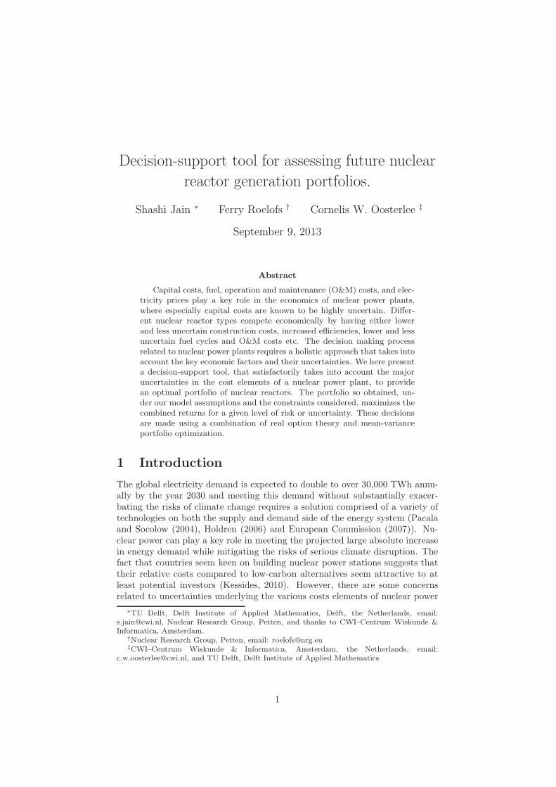
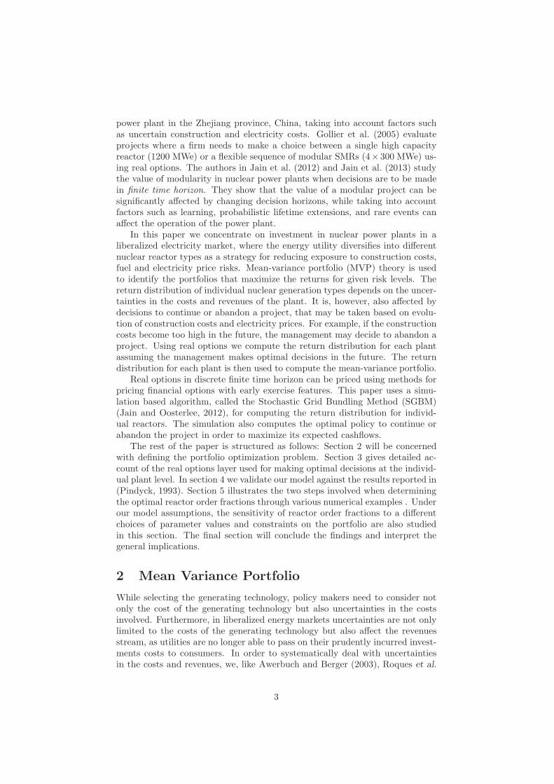
We would like to emphasize the role of real options in computing the netexpected cashflow and its distribution when a firm is flexible to take decisionsduring the course of construction and operation of the reactor. If the underlyingstochastic factors like expected cost of completion turn unfavourable in thefuture the firm uses its discretion to abandon the project9 in such a way that thenet expected cashflow is maximized. Figure 3 compares the cashflow distributionwhen (a) the firm doesn’t have the flexibility to change its decision in the futureand continues with the construction of the reactor irrespective of whether thescenario is favourable or not, (b) the firm has the flexibility to change its decisionand continues or abandons the project following the policy computed usingSGBM. It can be seen that the option to abandon the project under unfavourableprice scenarios reduces the possibility of extreme losses. Table 4 compares theexpectation and standard deviation of the net cashflow for the above two cases.

9It is assumed that the firm behaves rationally throughout the life cycle of constructionand operation of a nuclear power plant, although there is some empirical evidence whichsuggests that management might act otherwise when sunk costs are involved, for examplesee “Throwing good money after bad ? : Nuclear power plant investment decisions and therelevance of sunk costs”by Bondt and Makhija (1988) .

14

−2000−1500

−1000−500

0500

1000

0

0.01

0.02

0.03

0.04

0.05

0.06

0.07

0.08

Cashflow

Fre

quen

cy

FlexibleInFlexible

Figure 3: Distribution of net cashflow when the firm has flexible and inflexible decision toabandon the project in future. The policy, when early abandonment is possible, is computedusing SGBM. Same set of scenario paths are used for the two cases.

Inflexible Flexible caseCase (SGBM)

Expectednet cashflow ($/kWe) 186 221

Standarddeviation 600 500

Table 4: The expected value and standard deviation of the net cashflow corresponding tothe distribution in Figure 3. The reactor parameters are taken from Table 2 and [β, γ] valuesare [0.59 0.07], respectively.

15

2 4 6 8 10 12 14 16 18 20 220

0.005

0.01

0.015

0.02

0.025

0.03

0.035

0.04

0.045

Time(years)

Fra

ctio

n of

Pat

hs

Figure 4: Fraction of paths abandoned at different time steps, when the policy from SGBMis followed, corresponding to the case considered in Table 4.

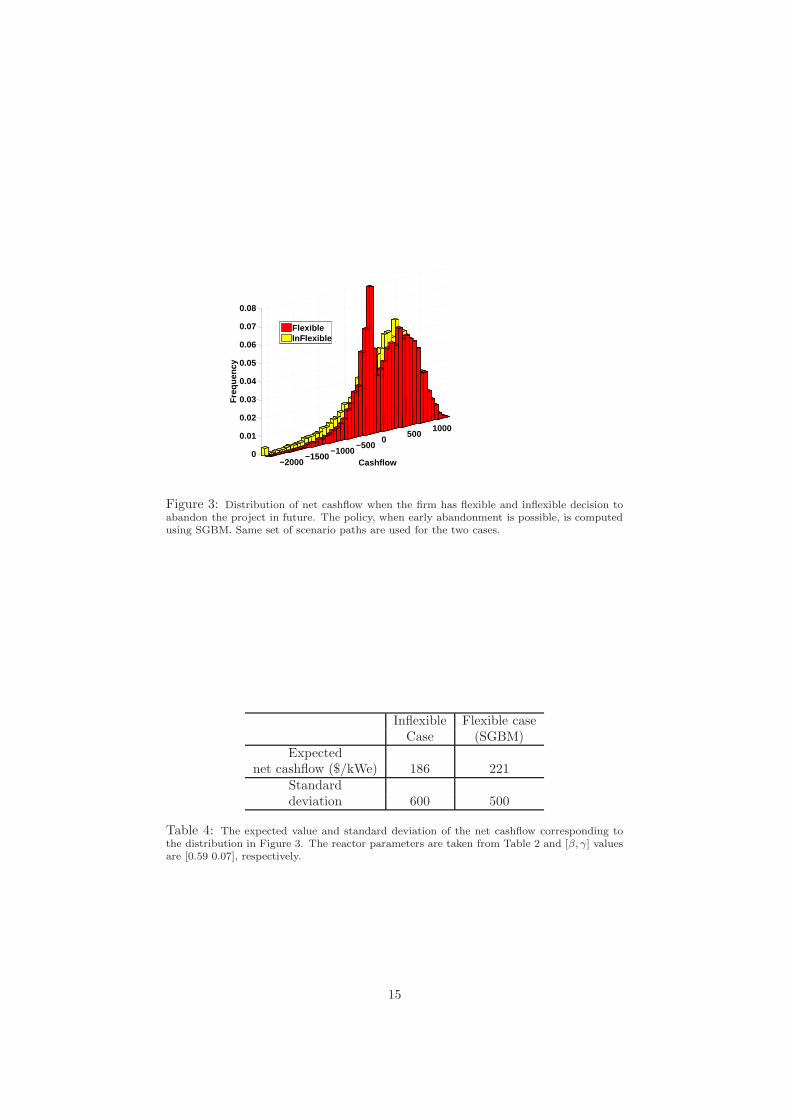
Figure 4 shows the fraction of scenario paths for which the project is aban-doned at different time steps when the policy from SGBM is followed for theabove case. It’s more likely for a project to be abandoned in its early phases thanin later stages. As the project commences the remaining expected constructioncosts (due to the ongoing investment) and also the remaining expected time tofinish the construction reduce while the anticipated revenues increase (as therevenues are expected to start flowing in relatively sooner, which implies theyare discounted less), which reduces the chance of the project being abandoned.

5 Numerical Examples

In this section we illustrate by various examples the two steps involved in de-ciding the optimal mix of NPPs for a power utility (or country or otherwise).We consider a more realistic case, where not only the costs are uncertain butalso the market price of electricity. We analyze the real option value, optimaldecision rules to start, continue or abandon the construction of a reactor, distri-bution of costs and cashflows obtained following the optimal policy for differentreactors. Finally, based on the expected net cashflow and its distribution, wefind the optimal reactor order fraction for the different reactors considered.

5.1 Choice of nuclear power plants

In this section we discuss the economics of different nuclear reactors we considerfor determining an optimal portfolio in energy generation planning. Here, notonly the expected costs of completion of the reactors are uncertain, but alsothe source of revenues, i.e. the electricity prices. The optimal decisions do notonly depend upon the expected costs of the reactor but also on the presentmarket price of electricity. Under our model assumption, the construction ofan unfinished reactor continues as long as the expected cost of completion isbelow some critical value and the electricity prices are above the correspondingthreshold electricity price. For a given expected construction cost if the presentelectricity price (per annum) falls below a threshold the expected net cashflow

16

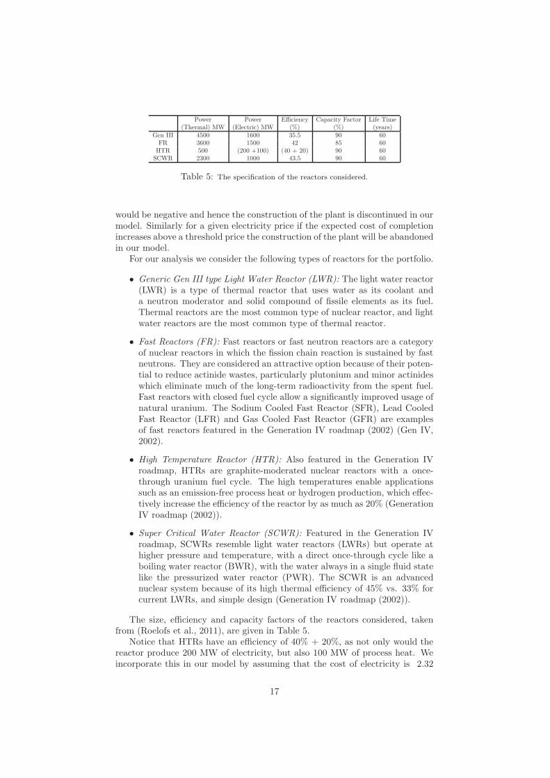
Power Power Efficiency Capacity Factor Life Time(Thermal) MW (Electric) MW (%) (%) (years)

Gen III 4500 1600 35.5 90 60FR 3600 1500 42 85 60HTR 500 (200 +100) (40 + 20) 90 60SCWR 2300 1000 43.5 90 60

Table 5: The specification of the reactors considered.

would be negative and hence the construction of the plant is discontinued in ourmodel. Similarly for a given electricity price if the expected cost of completionincreases above a threshold price the construction of the plant will be abandonedin our model.

For our analysis we consider the following types of reactors for the portfolio.

• Generic Gen III type Light Water Reactor (LWR): The light water reactor(LWR) is a type of thermal reactor that uses water as its coolant anda neutron moderator and solid compound of fissile elements as its fuel.Thermal reactors are the most common type of nuclear reactor, and lightwater reactors are the most common type of thermal reactor.

• Fast Reactors (FR): Fast reactors or fast neutron reactors are a categoryof nuclear reactors in which the fission chain reaction is sustained by fastneutrons. They are considered an attractive option because of their poten-tial to reduce actinide wastes, particularly plutonium and minor actinideswhich eliminate much of the long-term radioactivity from the spent fuel.Fast reactors with closed fuel cycle allow a significantly improved usage ofnatural uranium. The Sodium Cooled Fast Reactor (SFR), Lead CooledFast Reactor (LFR) and Gas Cooled Fast Reactor (GFR) are examplesof fast reactors featured in the Generation IV roadmap (2002) (Gen IV,2002).

• High Temperature Reactor (HTR): Also featured in the Generation IVroadmap, HTRs are graphite-moderated nuclear reactors with a once-through uranium fuel cycle. The high temperatures enable applicationssuch as an emission-free process heat or hydrogen production, which effec-tively increase the efficiency of the reactor by as much as 20% (GenerationIV roadmap (2002)).

• Super Critical Water Reactor (SCWR): Featured in the Generation IVroadmap, SCWRs resemble light water reactors (LWRs) but operate athigher pressure and temperature, with a direct once-through cycle like aboiling water reactor (BWR), with the water always in a single fluid statelike the pressurized water reactor (PWR). The SCWR is an advancednuclear system because of its high thermal efficiency of 45% vs. 33% forcurrent LWRs, and simple design (Generation IV roadmap (2002)).

The size, efficiency and capacity factors of the reactors considered, takenfrom (Roelofs et al., 2011), are given in Table 5.

Notice that HTRs have an efficiency of 40% + 20%, as not only would thereactor produce 200 MW of electricity, but also 100 MW of process heat. Weincorporate this in our model by assuming that the cost of electricity is 2.32

17

200 400 600 800 1000 1200 1400 1600

55%

60%

65%

70%

75%

80%

85%

90%

95%

100%

Size MWe

Mod

ular

Con

stru

ctio

n F

acto

r

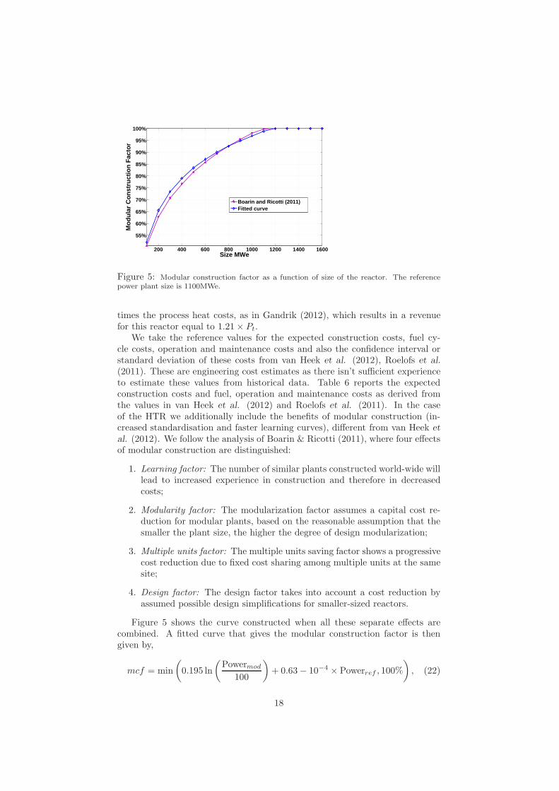
Boarin and Ricotti (2011)Fitted curve

Figure 5: Modular construction factor as a function of size of the reactor. The referencepower plant size is 1100MWe.

times the process heat costs, as in Gandrik (2012), which results in a revenuefor this reactor equal to 1.21× Pt.

We take the reference values for the expected construction costs, fuel cy-cle costs, operation and maintenance costs and also the confidence interval orstandard deviation of these costs from van Heek et al. (2012), Roelofs et al.

(2011). These are engineering cost estimates as there isn’t sufficient experienceto estimate these values from historical data. Table 6 reports the expectedconstruction costs and fuel, operation and maintenance costs as derived fromthe values in van Heek et al. (2012) and Roelofs et al. (2011). In the caseof the HTR we additionally include the benefits of modular construction (in-creased standardisation and faster learning curves), different from van Heek et

al. (2012). We follow the analysis of Boarin & Ricotti (2011), where four effectsof modular construction are distinguished:

1. Learning factor: The number of similar plants constructed world-wide willlead to increased experience in construction and therefore in decreasedcosts;

2. Modularity factor: The modularization factor assumes a capital cost re-duction for modular plants, based on the reasonable assumption that thesmaller the plant size, the higher the degree of design modularization;

3. Multiple units factor: The multiple units saving factor shows a progressivecost reduction due to fixed cost sharing among multiple units at the samesite;

4. Design factor: The design factor takes into account a cost reduction byassumed possible design simplifications for smaller-sized reactors.

Figure 5 shows the curve constructed when all these separate effects arecombined. A fitted curve that gives the modular construction factor is thengiven by,

mcf = min

(

0.195 ln

(

Powermod

100

)

+ 0.63− 10−4 × Powerref , 100%

)

, (22)

18

Expected ExpectedReactor construction cost Fuel and O&M cost

e/kWe e/kWe/aGeneric 2900 140

Gen III LWR (320) (35)FR 4600 185

(580) (35)HTR 3600 165

(750) (35)SCWR 3400 140

(400) (33)

Table 6: Expected construction, fuel and O&M costs for different reactors considered. Thevalues in brackets are standard deviations of these costs.

where Powerref is 1100 MWe and Powermod is on the x-axis of figure 5. Fol-lowing equation (22) based on the assessment of Boarin and Ricotti (2011), themodularity construction factor would be 65.5% for a Powermod = 200 MWeHTR, which brings down the expected costs of construction of HTRs from 6100to 3600 e/kWe.

As the values reported in Table 6 are “engineering estimates ”the uncertaintyin these values can primarily be attributed to technical uncertainty. Whenonly technical uncertainties are involved the variance of the expected cost ofconstruction is given by (see Pindyck (1993)) :

Var(K) =

(

β2

2− β2

)

K2;

a relation we use to compute the corresponding value of β for different reactorsin the portfolio. The Brownian motions driving the input cost uncertainties(see section 3.1) for different reactors can be correlated to each other (and theeconomy), as raw material required and government regulations are similar fordifferent reactors, while technical uncertainties for different reactors are assumedto be uncorrelated. Table 7 summarizes the parameter choices related to Table6.

The real option value of the reactors and the distribution of the net cashflowunder optimal policy for construction and operation of the reactors, depends on,amongst others, the expected growth rate for electricity prices (µ∗

p), uncertaintyin electricity prices (σp), and the discount rate used (r)10. Table 8 gives valuesconsidered for these parameters. For the base case, values corresponding to therow ’Medium’ in Table 8 are taken, and the initial price of electricity Pt0 is setto 8.5 cents/kWh.

10As the Brownian motions dWγ , dWC , dWP may be correlated with the market, we cannotuse the risk-free interest rate for discounting, especially if spanning is not possible. We insteadconsider different discount rates which represent different levels of risk premiums added to therisk-free rate.

19

K0 = 2900 (e/kWe),γ=0.07,

Generic β = 0.15,GenIII expected construction time = 5 years,

C0 = 1.36 (cents/kWh),σC = 0.25;

K0 = 4600 (e/kWe),γ =0.07,

Generic β = 0.18,Fast Reactor expected construction time = 7 years,

C0 = 1.95 (cents/kWh),σC = 0.19;

K0 = 3600 (e/kWe),γ=0.07,

HTR β = 0.17,expected construction time = 4 years,

C0 = 1.70 (cents/kWh),σC = 0.22;

K0 = 3400 (e/kWe),γ = 0.07,

SCWR β = 0.16,expected construction time = 5 years,

C0 = 1.43 (cents/kWh),σC = 0.24;

Table 7: Initial expected cost of completion, input cost uncertainty parameter γ, technicaluncertainty parameter β, expected construction time, present value of combined O&M andfuel charges C0 and the corresponding volatility for different reactors. For all cases consideredwe assume the correlation coefficient ρ between WP and WC to be 0.5 and the growth ratein O&M costs, µ∗

C to be 0. The rate of investment I for each reactor is taken as their initialexpected construction costs divided by their expected construction times.

Growth rate Uncertainty Discount rateµ∗

p (% per annum) σp (% per annum) r (% per annum)

Low 0 10 6Medium 3 20 8High 5 30 10

Table 8: Values of electricity price growth rate µ∗p, uncertainty in electricity prices, σp and

discount rate r considered in various examples.

20

3600 3800 4000 4200 4400 4600 4800 5000 5200 5400150

200

250

300

350

400

450

500

550

Kt ($/kWe)

(Pt−C

t) ($

/kW

h/a)

ContinueAbandon

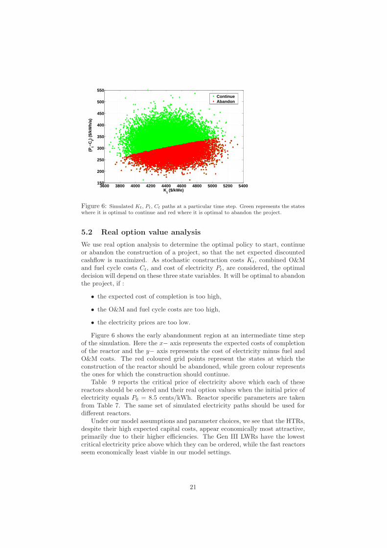
Figure 6: Simulated Kt, Pt, Ct paths at a particular time step. Green represents the stateswhere it is optimal to continue and red where it is optimal to abandon the project.

5.2 Real option value analysis

We use real option analysis to determine the optimal policy to start, continueor abandon the construction of a project, so that the net expected discountedcashflow is maximized. As stochastic construction costs Kt, combined O&Mand fuel cycle costs Ct, and cost of electricity Pt, are considered, the optimaldecision will depend on these three state variables. It will be optimal to abandonthe project, if :

• the expected cost of completion is too high,

• the O&M and fuel cycle costs are too high,

• the electricity prices are too low.

Figure 6 shows the early abandonment region at an intermediate time stepof the simulation. Here the x− axis represents the expected costs of completionof the reactor and the y− axis represents the cost of electricity minus fuel andO&M costs. The red coloured grid points represent the states at which theconstruction of the reactor should be abandoned, while green colour representsthe ones for which the construction should continue.

Table 9 reports the critical price of electricity above which each of thesereactors should be ordered and their real option values when the initial price ofelectricity equals P0 = 8.5 cents/kWh. Reactor specific parameters are takenfrom Table 7. The same set of simulated electricity paths should be used fordifferent reactors.

Under our model assumptions and parameter choices, we see that the HTRs,despite their high expected capital costs, appear economically most attractive,primarily due to their higher efficiencies. The Gen III LWRs have the lowestcritical electricity price above which they can be ordered, while the fast reactorsseem economically least viable in our model settings.

21

Type Critical electricity Option valueprice P ∗

0 P0 = 8.5 cents/kWhGen III LWR 4.0 3100

FR 6.25 875HTR 4.5 3500SCWR 4.7 2650

Table 9: Critical price of electricity P ∗t0

in (euro cents/kWh) above which the reactorsshould be ordered and their option values (in e/kWe) when the initial price of electricity is8.5 euro-cents/kWh. The reactor parameters are taken from Tables 7 and 8.

5.3 Optimal portfolio analysis

If a firm has to choose amongst the above reactors, solely based on their capitalcosts (Table 7), then their portfolio would contain only Generic Gen III typeLWRs, something also observed in practice. However, such a portfolio excludesthe role of uncertainties of cashflows for these reactors. Application of MVP the-ory takes into account not only the expected returns but also the uncertaintiesor risks associated with these returns.

An efficient frontier gives the optimal reactor order fraction for a portfoliodesigned to meet a given expected return while minimizing the uncertainties ofthese returns. In order to determine the efficient frontier the expected returnsand the covariance matrix of the returns from the reactors considered are re-quired. The distribution of returns for each reactor optimally constructed issampled by computing the returns along each simulated path.

The following constraints on the portfolio are considered:

• Budget constraint: Under a budget constraint, the optimal reactor orderfraction for every euro spent is computed. Returns corresponding to aeuro spent on a reactor are given by,

Ri(n) =Revenuei(n)− Costi(n)

Costi(n), (23)

and the constraint for the portfolio optimization problem is then:

J∑

i=1

wi = 1,

n = 1, . . . , N being the path index and i = 1, . . . , J indicate the differentreactors considered. The weights correspond to the fraction of moneyinvested in different reactors, which is then used to compute the reactororder fraction (per kWe) by taking into account the expected constructioncosts as reported in Table 7.

• Capacity constraint: Under a capacity constraint, the optimal reactororder fraction for every kWe of capacity ordered is computed. Returnscorresponding to a kWe ordered are given by,

Ri(n) = Revenuei(n)− Costi(n),

22

Gen III FR HTR SCWRExpected Return 1.3376 0.1863 1.0645 0.9744Stdev Return 1.2356 0.9046 0.9926 1.0527

Table 10: The expected return and its standard deviation per euro spent for the base case.

and the constraint for the portfolio optimization problem is:

J∑

i=1

wi = 1,

n = 1, . . . , N being the path index, and i = 1, . . . , J indicate the differ-ent reactors considered. The constraint implies here that reactor orderfractions should add up to a kWe.

For both constraints, the weights are additionally bounded as,

0 ≤ wi ≤ 1, i = 1, . . . , J,

which comes naturally from the fact that short selling is not possible here,and thus the weights cannot be negative.

The quadratic programming problem expressed by equation (5) is solvedusing the optimization toolbox of MATLAB, which solves general problems ofthe kind:

minw

1

2w⊤Qw + f ′w,

such that: Aw ≤ a,

Bw = b, (24)

L ≤ w ≤ U,

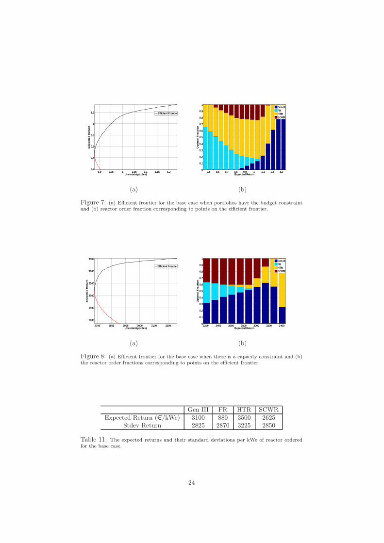
using the command w = quadprog(Q,f,A,a,B,b,L,U).Figure 7 displays the efficient frontier and the corresponding optimal reactor

order fraction when the portfolio has the budget constraint. The mean and stan-dard deviation of the simulated returns for the individual reactors are reportedin Table 10. Under our model assumptions and choice of parameter values, theGenIII LWRs have the highest expected returns (based on equation (23), whilethe FRs have the lowest returns per euro spent. However, the uncertainty ofreturns for FRs is lower than that for GenIII LWRs. An investor who wantsto minimize the uncertainty of returns and is willing to take a lower expectedreturn in order to do so, will choose a portfolio with more Gen IV type reactors.An investor who wants higher returns and is indifferent to the uncertainty ofreturns, will hold a portfolio with more Gen III type reactors.

Figure 8 shows the efficient frontier and optimal reactor order fraction corre-sponding to points on the optimal frontier, when the portfolios have the capacityconstraint. Expected returns and their standard deviations per kWe of reactorordered are reported in Table 11. We see that unlike the case with the budgetconstraint, where portfolios with high returns were dominated by Gen III LWRs,here portfolios with higher expected returns are dominated by both HTR andGenIII LWRs. This difference can be explained as the returns in equation (23)are scaled by the individual reactor costs.

23

0.9 0.95 1 1.05 1.1 1.15 1.20.2

0.4

0.6

0.8

1

1.2

Uncertainty(stdev)

Exp

ect

ed

Re

turn

Efficient Frontier

(a)

0.5 0.6 0.7 0.8 0.9 1 1.1 1.2 1.30

0.1

0.2

0.3

0.4

0.5

0.6

0.7

0.8

0.9

1

Expected Return

Op

tima

l Fra

ctio

n

Gen IIIFRHTRSCWR

(b)

Figure 7: (a) Efficient frontier for the base case when portfolios have the budget constraintand (b) reactor order fraction corresponding to points on the efficient frontier.

2700 2800 2900 3000 3100 3200

1000

1500

2000

2500

3000

3500

Uncertainty(stdev)

Exp

ect

ed

Re

turn

Efficient Frontier

(a)

2200 2400 2600 2800 3000 3200 34000

0.1

0.2

0.3

0.4

0.5

0.6

0.7

0.8

0.9

1

Expected Return

Op

tima

l Fra

ctio

n

Gen IIIFRHTRSCWR

(b)

Figure 8: (a) Efficient frontier for the base case when there is a capacity constraint and (b)the reactor order fractions corresponding to points on the efficient frontier.

Gen III FR HTR SCWRExpected Return (e/kWe) 3100 880 3500 2625

Stdev Return 2825 2870 3225 2850

Table 11: The expected returns and their standard deviations per kWe of reactor orderedfor the base case.

24

1000 1500 2000 2500 3000 3500 4000 4500 50000

1000

2000

3000

4000

5000

6000

7000

Uncertainty(stdev)

Exp

ecte

d R

etur

n (p

er k

We)

r=10%r=8%r=6%

Figure 9: Efficient frontiers for varying discount rates. Parameter values are taken fromTables 7 and 8.

5.4 Portfolio sensitivity

In addition to the constraints on the portfolio, the choice of parameter valuesaffects the structure of the optimal portfolio. We study the optimal portfoliofor varying parameter values, which gives an intuition about the portfolio’ssensitivity with respect to these parameters. In particular, we consider thefollowing cases:

• Different discount rates r, with other parameters constant.

• Varying electricity price growth rates µ∗p, with other parameters constant.

• Varying uncertainties in electricity prices σp, with other parameters con-stant.

From here on, we only consider portfolios that have capacity constraints.

Varying discount rates

For our reference case, we considered a discount rate of 8% per annum. We ex-amine the portfolios sensitivity to varying discount rates. A change in discountrate affects the expected revenues, costs and the optimal investment strategy,which in turn affects the returns. This makes the discount rate an importantparameter while computing the efficient frontier and corresponding optimal re-actor order fractions.

Figure 9 shows the efficient frontier for low, medium and high discount rates,with corresponding values taken from Table 8. Lowering the discount rate canhelp realize higher expected returns, although at increased uncertainty (vari-ance) in returns. Although both the expected returns and the variance of returnsincreases, however, the increase in the expected returns is more significant thanincrease in the variance of returns. Therefore, reactors with higher expectedreturns would then be more favoured in the mean-variance portfolio.

The optimal reactor order fractions corresponding to the points on the effi-cient frontier are shown in Figure 10. Under our model assumptions and param-eter choices, we see that lowering discount rates results in a portfolio dominatedby reactors having greater expected returns, while higher discount rates resultin a portfolio where reactors with lower uncertainties dominate.

25

200 400 600 800 1000 1200 1400 1600 18000

0.2

0.4

0.6

0.8

1

Expected Return

Op

tim

al F

ractio

n

Gen IIIFRHTRSCWR

(a)

2400 2600 2800 3000 3200 34000

0.1

0.2

0.3

0.4

0.5

0.6

0.7

0.8

0.9

1

Expected Return

Op

tima

l Fra

ctio

n

Gen IIIFRHTRSCWR

(b)

5200 5400 5600 5800 6000 62000

0.2

0.4

0.6

0.8

1

Expected Return

Op

tim

al F

ractio

n

Gen IIIFRHTRSCWR

(c)

Figure 10: Optimal reactor order fractions when (a) r = 10%, (b) r = 8%, and (c) r = 6%.

Parameter values are taken from Tables 7 and 8.

1600 1800 2000 2200 2400 2600 2800 3000 3200 3400 36000

500

1000

1500

2000

2500

3000

3500

4000

4500

Uncertainty(stdev)

Exp

ecte

d R

etur

n

µ∗

p= 5%

µ∗

p= 3%

µ∗

p= 0%

Figure 11: Efficient frontier for varying electricity price growth rate, where the reactorspecific parameters are taken from Table 7, and economic parameters from Table 8.

Varying electricity price growth rates

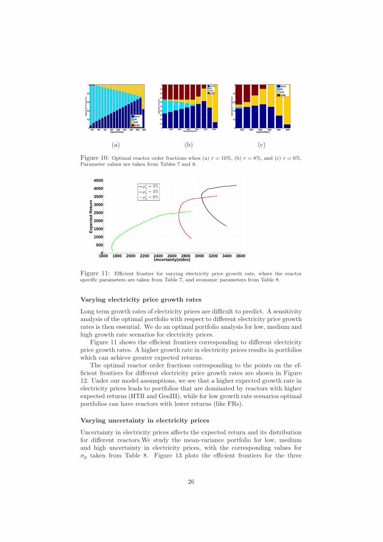
Long term growth rates of electricity prices are difficult to predict. A sensitivityanalysis of the optimal portfolio with respect to different electricity price growthrates is then essential. We do an optimal portfolio analysis for low, medium andhigh growth rate scenarios for electricity prices.

Figure 11 shows the efficient frontiers corresponding to different electricityprice growth rates. A higher growth rate in electricity prices results in portfolioswhich can achieve greater expected returns.

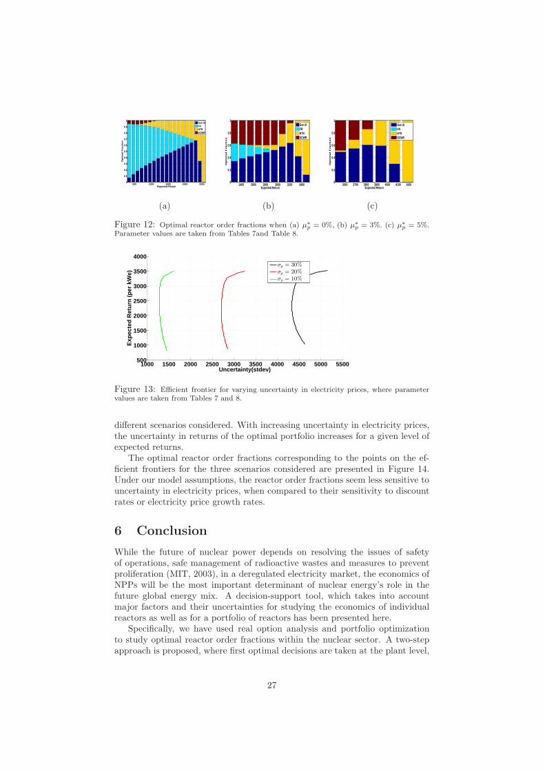
The optimal reactor order fractions corresponding to the points on the ef-ficient frontiers for different electricity price growth rates are shown in Figure12. Under our model assumptions, we see that a higher expected growth rate inelectricity prices leads to portfolios that are dominated by reactors with higherexpected returns (HTR and GenIII), while for low growth rate scenarios optimalportfolios can have reactors with lower returns (like FRs).

Varying uncertainty in electricity prices

Uncertainty in electricity prices affects the expected return and its distributionfor different reactors.We study the mean-variance portfolio for low, mediumand high uncertainty in electricity prices, with the corresponding values forσp taken from Table 8. Figure 13 plots the efficient frontiers for the three

26

500 1000 1500 2000 25000

0.1

0.2

0.3

0.4

0.5

0.6

0.7

0.8

0.9

1

Expected Return

Op

tima

l Fra

ctio

n

Gen IIIFRHTRSCWR

(a)

2400 2600 2800 3000 3200 34000

0.2

0.4

0.6

0.8

1

Expected Return

Op

tim

al F

ractio

n

Gen IIIFRHTRSCWR

(b)

3600 3700 3800 3900 4000 4100 42000

0.2

0.4

0.6

0.8

1

Expected Return

Op

tim

al F

ractio

n

Gen IIIFRHTRSCWR

(c)

Figure 12: Optimal reactor order fractions when (a) µ∗p = 0%, (b) µ∗

p = 3%. (c) µ∗p = 5%.

Parameter values are taken from Tables 7and Table 8.

1000 1500 2000 2500 3000 3500 4000 4500 5000 5500500

1000

1500

2000

2500

3000

3500

4000

Uncertainty(stdev)

Exp

ecte

d R

etur

n (p

er k

We)

σp = 30%

σp = 20%

σp = 10%

Figure 13: Efficient frontier for varying uncertainty in electricity prices, where parametervalues are taken from Tables 7 and 8.

different scenarios considered. With increasing uncertainty in electricity prices,the uncertainty in returns of the optimal portfolio increases for a given level ofexpected returns.

The optimal reactor order fractions corresponding to the points on the ef-ficient frontiers for the three scenarios considered are presented in Figure 14.Under our model assumptions, the reactor order fractions seem less sensitive touncertainty in electricity prices, when compared to their sensitivity to discountrates or electricity price growth rates.

6 Conclusion

While the future of nuclear power depends on resolving the issues of safetyof operations, safe management of radioactive wastes and measures to preventproliferation (MIT, 2003), in a deregulated electricity market, the economics ofNPPs will be the most important determinant of nuclear energy’s role in thefuture global energy mix. A decision-support tool, which takes into accountmajor factors and their uncertainties for studying the economics of individualreactors as well as for a portfolio of reactors has been presented here.

Specifically, we have used real option analysis and portfolio optimizationto study optimal reactor order fractions within the nuclear sector. A two-stepapproach is proposed, where first optimal decisions are taken at the plant level,

27

2500 2600 2700 2800 2900 3000 3100 3200 3300 34000

0.1

0.2

0.3

0.4

0.5

0.6

0.7

0.8

0.9

1

Expected Return

Op

tima

l Fra

ctio

n

Gen IIIFRHTRSCWR

(a)

2200 2400 2600 2800 3000 3200 34000

0.1

0.2

0.3

0.4

0.5

0.6

0.7

0.8

0.9

1

Expected Return

Op

tima

l Fra

ctio

n

Gen IIIFRHTRSCWR

(b)

2400 2600 2800 3000 3200 34000

0.1

0.2

0.3

0.4

0.5

0.6

0.7

0.8

0.9

1

Expected Return

Op

tima

l Fra

ctio

n

Gen IIIFRHTRSCWR

(c)

Figure 14: Optimal reactor order fractions when (a) σp = 10%, (b) σp = 20%, and (c)σp = 30%. Parameter values are taken from Tables 7 and 8.

and then the resulting distribution of returns for each reactor-type are used asinputs to a portfolio optimization problem solved using MVP theory. The maincontribution on the methodological side can be stated as:

• The method adequately accounts for uncertain reactor construction costsand schedule, and reflects their effect on the return distribution for differ-ent reactors.

• An optimal policy for continuing the construction or abandoning theproject is computed taking into account the uncertainties in constructioncosts, electricity prices and O&M and fuel cycle costs involved.

• A detailed study on optimal portfolios based on MVP theory is conducted.

• The effect of different constraints on portfolio diversification is studied.

• The sensitivity of the optimal portfolio with respect to electricity pricegrowth rates, uncertainty in electricity prices and discount rates is studied.

It should be emphasized here that, although careful attention has been paidto choose realistic parameter values for the reactors considered, however, themain focus of the paper is to illustrate a methodology that accounts for the var-ious economic uncertainties related to nuclear power plants. Under our modelassumptions, it has been shown that certain scenarios lead to portfolios that aredominated by Generation IV type reactors, while others result in conventionalGen III type LWRs being the dominant ones. Following the methodology de-scribed here can be useful when decisions related to reactor order fraction needto be made.

As possible future direction of research, the portfolio optimization stepshould in addition to the variance of the returns also consider other risk mea-sures, such as, value at risk and conditional value at risk. The resulting portfolioswill not only minimize the variance of the returns but will also avoid reactorswhich are likely to be abandoned in the future.

References

K. J. Arrow and A. C. Fisher. Environmental preservation, uncertainty, andirreversibility. The Quarterly Journal of Economics, 88(2):312–319, 1974.

28

S. Awerbuch and M. Berger. Energy security and diversity in the EU: A mean-variance portfolio approach. IEA Research Paper, 2003.

M. T. Barlow. A diffusion model for electricity prices. Mathematical Finance,12(4):287–298, 2002.

S. Boarin, G. Locatelli, M. Mancini, and M. E. Ricotti. Financial case studies onsmall-and medium-size modular reactors. Nuclear technology, 178(2):218–232,2012.

E. Commission. The sustainable nuclear energy technology platform. SpecialReport, 2007.

W. F. De Bondt and A. K. Makhija. Throwing good money after bad?: Nuclearpower plant investment decisions and the relevance of sunk costs. Journal ofEconomic Behavior & Organization, 10(2):173–199, 1988.

J. Deutch, E. Moniz, S. Ansolabehere, M. Driscoll, P. Gray, J. Holdren,P. Joskow, R. Lester, and N. Todreas. The future of nuclear power. anMIT Interdisciplinary Study, http://web. mit. edu/nuclearpower, 2003.

I. Fortin, S. Fuss, J. Hlouskova, N. Khabarov, M. Obersteiner, and J. Szolgayova.An integrated CVaR and real options approach to investments in the energysector. Technical report, Institute for Advanced Studies, 2007.

S. Fuss, J. Szolgayova, N. Khabarov, and M. Obersteiner. Renewables andclimate change mitigation: Irreversible energy investment under uncertaintyand portfolio effects. Energy Policy, 40(0):59 – 68, 2012.

A. M. Gandrik. HTGR application economic model users manual. Technicalreport, Idaho National Laboratory (INL), 2012.

R. Gen IV. US DOE Nuclear energy research advisory committee and thegeneration IV international forum. A technology roadmap for generation IVnuclear energy systems. gif002-00, december 2002, 2002.

C. Gollier, D. Proult, F. Thais, and G. Walgenwitz. Choice of nuclear powerinvestments under price uncertainty: valuing modularity. Energy Economics,27(4):667–685, 2005.

J. P. Holdren. The energy innovation imperative: Addressing oil dependence,climate change, and other 21st century energy challenges. Innovations, 1(2):3–23, 2006.

S. Jain and C. W. Oosterlee. The Stochastic Grid Bundling Method: Efficientpricing of Bermudan options and the Greeks. Available at SSRN 2293942,2012.

S. Jain, F. Roelofs, and C. W. Oosterlee. Valuing modular nuclear power plantsin finite time decision horizon. Energy Economics, 2012.

S. Jain, C. W. Oosterlee, and F. Roelofs. Construction strategies and lifetimeuncertainties for nuclear projects: A real option analysis. Nuclear Engineeringand Design, 2013. accepted.

29

J. Jansen, L. Beurskens, and X. Van Tilburg. Application of portfolio analysis tothe Dutch generating mix. Energy research Center at the Netherlands (ECN)report C-05-100, 2006.

I. N. Kessides. Nuclear power: Understanding the economic risks and uncer-tainties. Energy Policy, 38(8):3849 – 3864, 2010.

J. J. Lucia and E. S. Schwartz. Electricity prices and power derivatives: Evi-dence from the nordic power exchange. Review of Derivatives Research, 5(1):5–50, 2002.

H. Markowitz. Portfolio selection*. The Journal of Finance, 7(1):77–91, 1952.

R. C. Merton. An intertemporal capital asset pricing model. Econometrica:Journal of the Econometric Society, pages 867–887, 1973.

Y. Naito, R. Takashima, H. Kimura, and H. Madarame. Evaluating replacementproject of nuclear power plants under uncertainty. Energy Policy, 38(3):1321–1329, 2010.

OECD. Projected costs of generating electricity. Technical report, OECD, 2005.

S. Pacala and R. Socolow. Stabilization wedges: Solving the climate problemfor the next 50 years with current technologies. Science, 305(5686):968–972,2004.

D. Pilipovic. Energy risk: Valuing and managing energy derivatives, volume300. McGraw-Hill New York, 1998.

R. S. Pindyck. Investments of uncertain cost. Journal of Financial Economics,34(1):53–76, 1993.

F. Roelofs, J. Hart, and A. Van Heek. European new build and fuel cycles inthe 21st century. Nuclear Engineering and Design, 241(6):2307–2317, 2011.

F. A. Roques, D. M. Newbery, and W. J. Nuttall. Fuel mix diversificationincentives in liberalized electricity markets: A mean-variance portfolio theoryapproach. Energy Economics, 30(4):1831–1849, 2008.

G. Rothwell. A real options approach to evaluating new nuclear power plants.The Energy Journal, 0(1):87–54, 2006.

E. S. Schwartz. Patents and R&D as real options. Economic Notes, 33(1):23–54,2004.

J. Szolgayova, S. Fuss, N. Khabarov, and M. Obersteiner. A dynamic CVaR-portfolio approach using real options: an application to energy investments.European Transactions on Electrical Power, 21(6):1825–1841, 2011.

S. Thomas. The economics of nuclear power: analysis of recent studies. Availableat: www.psiru.org/reports/2005-09-E-Nuclear.pdf, 2005.

A. van Heek, F. Roelofs, and A. Ehlert. Cost estimation with G4-Econs forgeneration IV reactor designs. In GIF Symposium Proceedings, page 29, 2012.

L. Zhu. A simulation based real options approach for the investment evaluationof nuclear power. Comput. Ind. Eng., 63(3):585–593, 2012.

30