22
DECISION THEORY GOOD CAUSALITY BAD Philip Dawid University College London
| Date post: | 21-Dec-2015 |
| Category: |
Documents |
| View: | 218 times |
| Download: | 0 times |

DECISION THEORY GOOD
CAUSALITY BAD
DECISION THEORY GOOD
CAUSALITY BAD
Philip DawidUniversity College London

A SIMPLE PROBLEMA SIMPLE PROBLEM
• Randomised experiment
• Binary (0/1) treatment decision variable T
• Response variable Y
Define/measure “the effect of treatment”

Statistical ModelStatistical Model
• Measure effect of treatment by appropriate
comparison of distributions P0 and P1
– e.g. difference of expected responses01
)],(..[ 2tN~ge
• Specify/estimate conditional distributions
Pt for Y given T = t (t = 0, 1)
{ ( )}tY PE L Y:
• This is sufficient for optimal choice topt of T – choose to minimise expected loss
(Fisher)

T
Decision TreeDecision Tree
0
1
y
y
Y
Y
Y~P0
Y~P1
L(y)
L(y)
Influence DiagramInfluence Diagram
T YY~Ptt
LL(y)

• Split Y in two:
Y0 : response to T = 0
Y1 : response to T = 1
Potential Response ModelPotential Response Model
– necessarily unobservable!Y1 Y0
counterfactual/complementary
• Consider (for any unit) the pair Y = (Y0 , Y1)– with simultaneous existence and joint distribution
• Unit-level (individual) [random] causal effect
• Treatment “uncovers” pre-existing response: Y = YT (deterministic)

Potential Responses: ProblemsPotential Responses: Problems
NB: does not enter! – can never identify – does this matter??
• Corresponding statistical model:
• PR model:

Potential Responses: ProblemsPotential Responses: Problems
201 )1(2)var( YY
Under PR model:
)()1()|( 0111101 yyYYYE
We can not identify the variance of the ICE
We can not identify the (counterfactual) ICE after observing response to treatment
1 0( / )E Y Y depends on We can not estimate a “ratio” ICE

OBSERVATIONAL STUDYOBSERVATIONAL STUDY
• Treatment decision taken may be associated with patient’s state of health
• What assumptions are required to make causal inferences?
• When/how can such assumptions be justified?

TY Y=
1 2( , )Y Y=Y
Potential Response ModelPotential Response Model
– treatment independent of potential responses
Y
Y
T~ TT P
?
),(
~
T Y
“Ignorable treatment assignment”
(determined)(observational distribution)
(e.g., bivariate normal)
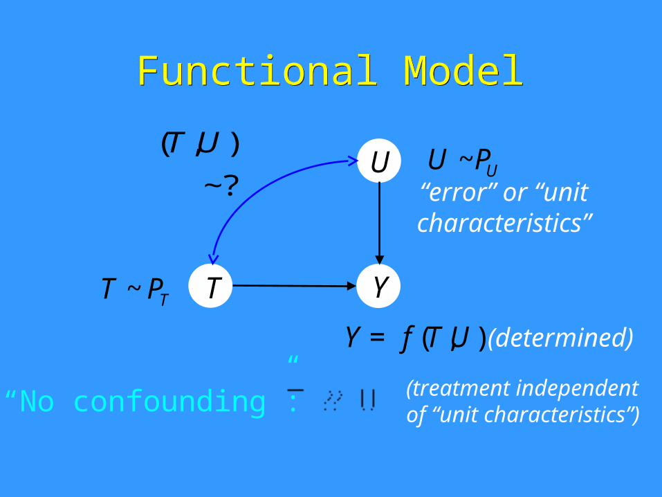
T Y
U
( , )Y f T U=
Functional ModelFunctional Model
TPT ~
~ UU P( , )
?
T U
~
“No confounding”: (treatment independent of “unit characteristics”)
(determined)
“error” or “unit characteristics”

CommentsComments
• Value of Y = (Y0, Y1) on any unit implicitly supposed the same in observational and experimental regimes (as well as for both choices of T )
• How are we to judge independence of T from Y ?

• Introduce explicit “treatment regime indicator” variable FT
• Values:FT = 0 : Assign treatment 0 ( T = 0)
FT = 1 : Assign treatment 1 ( T = 1)
FT = : Just observe
• “Ignorable treatment assignment”: – identity of observational and experimental
distributions for Y | T :
Statistical Decision ModelStatistical Decision Model

FT T
Influence DiagramInfluence Diagram
Y/1/01/0
),(| TFTY
b
TT PFT ~)(|
),(),(|.. 2 tT N~FtTYge
Absence of arrow b expresses
(probabilistic, not functional, relationships)

FT T
Cannot reverse arrow!Cannot reverse arrow!
Y
now expresses
rather than

DYNAMIC TREATMENT REGIMES
DYNAMIC TREATMENT REGIMES
YL1L0 A0 A1
time
observe observe observeact act
Distribution of Y under ?
Consider (deterministic) treatment regime :

PR ApproachPR Approach
“Consistency”:
For each regime have potential intermediate and response variables:
– if history to date consistent with , so is next observable

“Sequential Ignorability”“Sequential Ignorability”
– actions independent of future potential observables, given current (consistent) history
For each regime and all possible (l0, l1):
– when valid, allows estimation of distribution of any from observational data
– by “G-computation” formula

• Values include various (now possibly randomised) experimental regimes and observational regime
Decision ApproachDecision Approach
• Introduce explicit “dynamic regime indicator” variable G

Sequential IgnorabilitySequential Ignorability
Conditional distribution of each observable, given history, is the same under all regimes:

L1
G
Influence DiagramInfluence Diagram
L0 A0 A1 Y

CONCLUSIONSCONCLUSIONS
• Causal models based on potential responses incorporate untestable assumptions
• At best we are carrying dead wood
• At worst we can get different inferences for observationally equivalent models
• Standard probabilistic/ statistical/ decision-theoretic methods are clearer, more straightforward, and less prone to error

Further ReadingFurther Reading• Dawid, A. P. (2000). Causal inference without counterfactuals (with
Discussion). J. Amer. Statist. Ass. 95, 407– 448.
• Dawid, A. P. (2002). Influence diagrams for causal modelling and inference. Intern. Statist. Rev. 70, 161– 189. Corrigenda, ibid., 437.
• Dawid, A. P. (2003). Causal inference using influence diagrams: The problem of partial compliance (with Discussion). In Highly Structured Stochastic Systems, edited by Peter J. Green, Nils L. Hjort and Sylvia Richardson. Oxford University Press, 45 – 81.
• Dawid, A. P. (2004). Probability, causality and the empirical world: A Bayes–de Finetti–Popper–Borel synthesis. Statistical Science 19, 44 – 57.
• Dawid, A. P. and Didelez, V. (2005). Identifying the consequences of dynamic treatment strategies. Research Report 262, Department of Statistical Science, University College London.


