50
Decision Tree Learning - ID3
| Date post: | 14-Dec-2015 |
| Category: |
Documents |
| Upload: | micaela-beanland |
| View: | 273 times |
| Download: | 4 times |

Decision Tree Learning - ID3
Decision tree examples
ID3 algorithm Occam Razor Top-Down Induction in Decision Trees Information Theory gain from property P
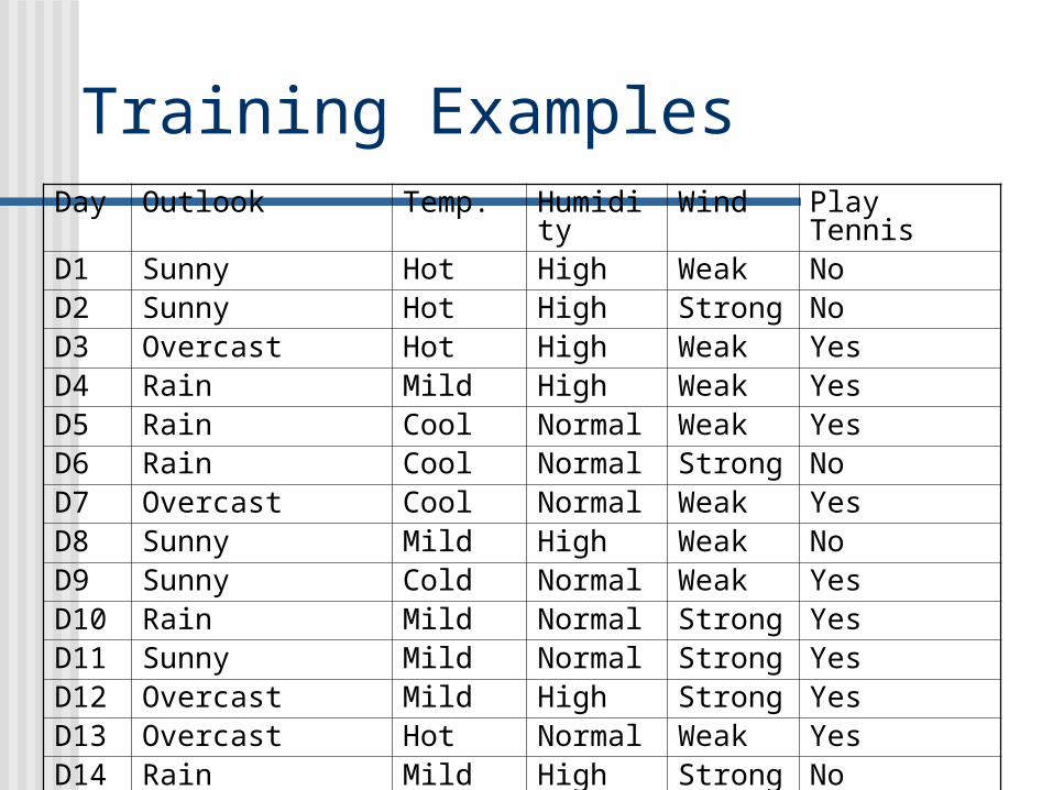
Training ExamplesDay Outlook Temp. Humidity Wind Play TennisD1 Sunny Hot High Weak NoD2 Sunny Hot High Strong NoD3 Overcast Hot High Weak YesD4 Rain Mild High Weak YesD5 Rain Cool Normal Weak YesD6 Rain Cool Normal Strong NoD7 Overcast Cool Normal Weak YesD8 Sunny Mild High Weak NoD9 Sunny Cold Normal Weak YesD10 Rain Mild Normal Strong YesD11 Sunny Mild Normal Strong YesD12 Overcast Mild High Strong YesD13 Overcast Hot Normal Weak YesD14 Rain Mild High Strong No

Decision Tree for PlayTennisOutlook
Sunny Overcast Rain
Humidity
High Normal
Wind
Strong Weak
No Yes
Yes
YesNo
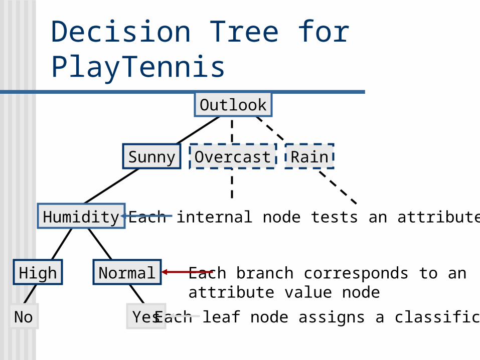
Decision Tree for PlayTennisOutlook
Sunny Overcast Rain
Humidity
High Normal
No Yes
Each internal node tests an attribute
Each branch corresponds to anattribute value node
Each leaf node assigns a classification
No
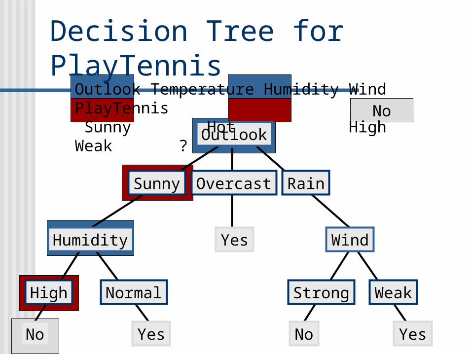
Decision Tree for PlayTennis
Outlook
Sunny Overcast Rain
Humidity
High Normal
Wind
Strong Weak
No Yes
Yes
YesNo
Outlook Temperature Humidity Wind PlayTennis Sunny Hot High Weak ?
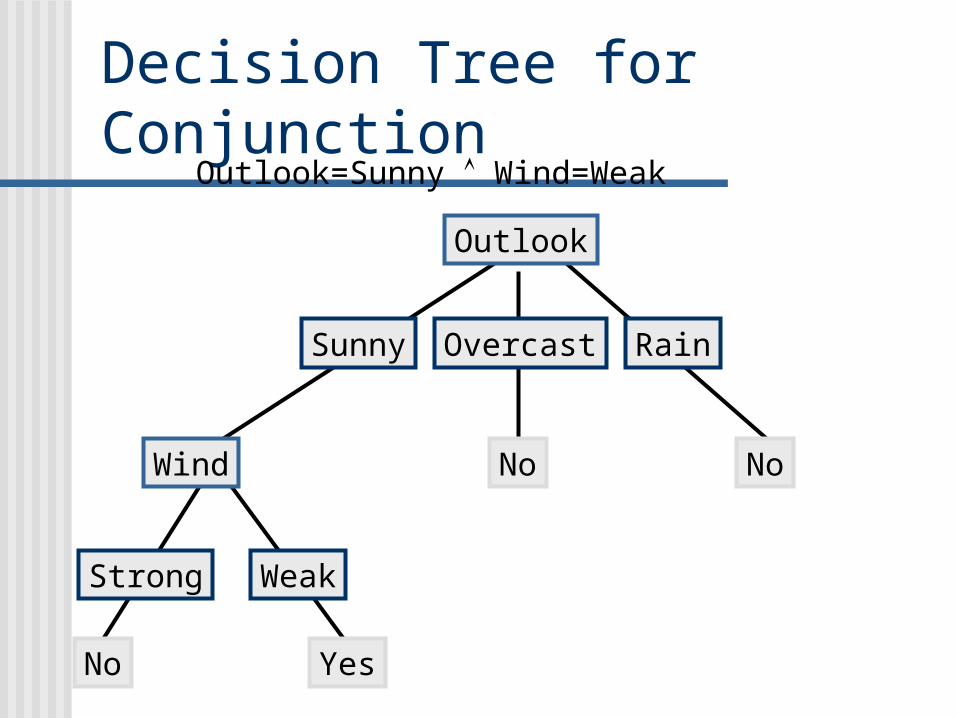
Decision Tree for Conjunction
Outlook
Sunny Overcast Rain
Wind
Strong Weak
No Yes
No
Outlook=Sunny Wind=Weak
No
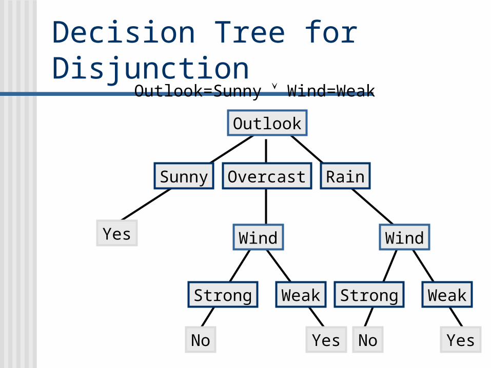
Decision Tree for Disjunction
Outlook
Sunny Overcast Rain
Yes
Outlook=Sunny Wind=Weak
Wind
Strong Weak
No Yes
Wind
Strong Weak
No Yes
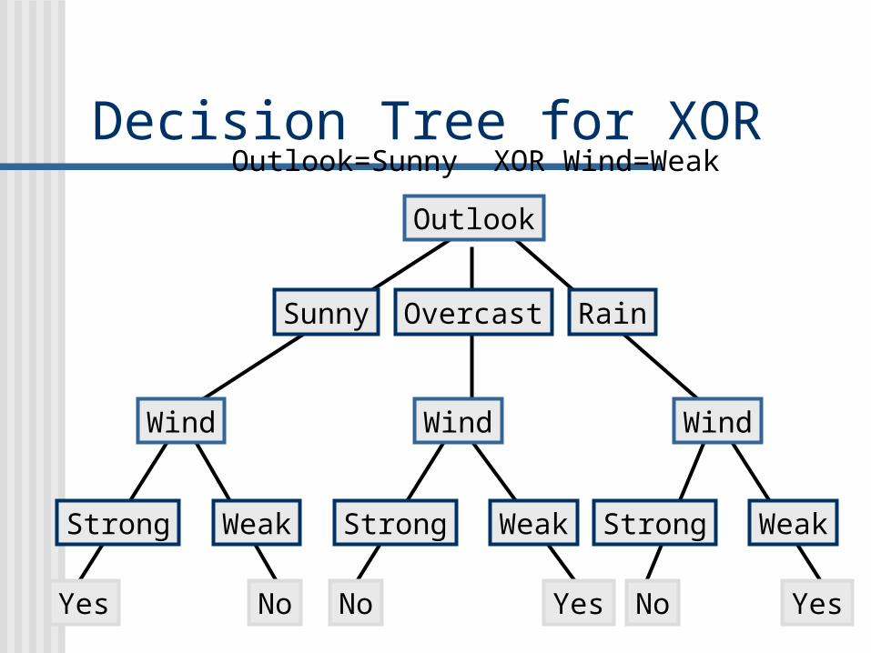
Decision Tree for XOR
Outlook
Sunny Overcast Rain
Wind
Strong Weak
Yes No
Outlook=Sunny XOR Wind=Weak
Wind
Strong Weak
No Yes
Wind
Strong Weak
No Yes
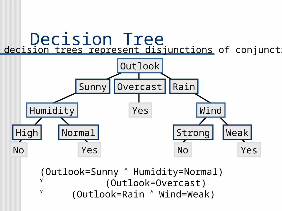
Decision Tree
Outlook
Sunny Overcast Rain
Humidity
High Normal
Wind
Strong Weak
No Yes
Yes
YesNo
• decision trees represent disjunctions of conjunctions
(Outlook=Sunny Humidity=Normal) (Outlook=Overcast) (Outlook=Rain Wind=Weak)
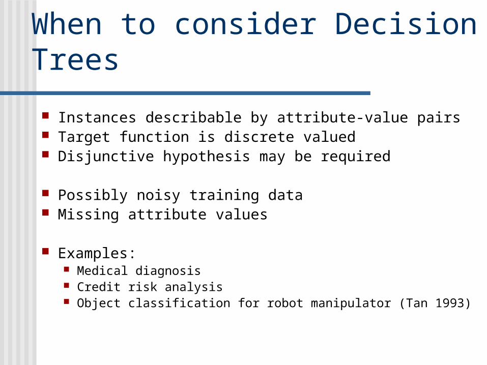
When to consider Decision Trees
Instances describable by attribute-value pairs Target function is discrete valued Disjunctive hypothesis may be required
Possibly noisy training data Missing attribute values
Examples: Medical diagnosis Credit risk analysis Object classification for robot manipulator (Tan 1993)

Zur Anzeige wird der QuickTime™ Dekompressor „TIFF (LZW)“
benötigt.

Zur Anzeige wird der QuickTime™ Dekompressor „TIFF (LZW)“
benötigt.

Zur Anzeige wird der QuickTime™ Dekompressor „TIFF (LZW)“
benötigt.

Zur Anzeige wird der QuickTime™ Dekompressor „TIFF (LZW)“
benötigt.

Decision tree for credit risk assessment
Zur Anzeige wird der QuickTime™ Dekompressor „TIFF (LZW)“
benötigt.
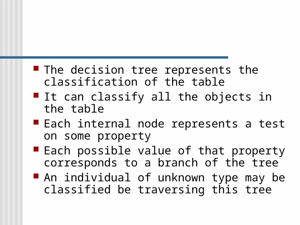
The decision tree represents the classification of the table
It can classify all the objects in the table Each internal node represents a test on some
property Each possible value of that property
corresponds to a branch of the tree An individual of unknown type may be classified
be traversing this tree
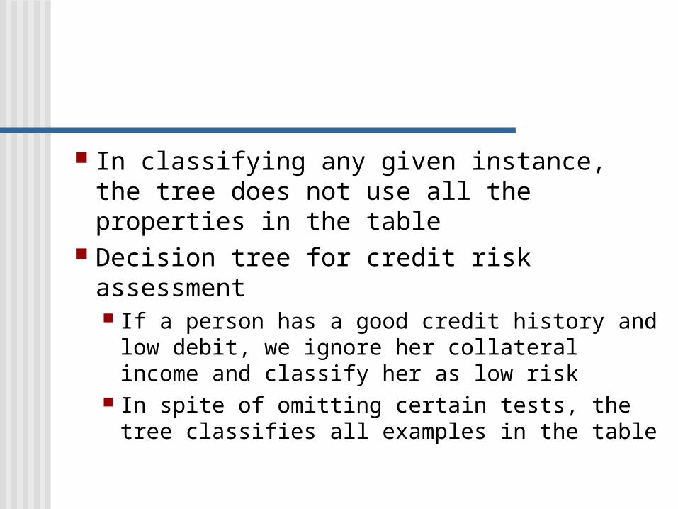
In classifying any given instance, the tree does not use all the properties in the table
Decision tree for credit risk assessment If a person has a good credit history and low
debit, we ignore her collateral income and classify her as low risk
In spite of omitting certain tests, the tree classifies all examples in the table

In general, the size of a tree necessary to classify a given set of examples varies according to the order with which properties (=attributes) are tested
Given a set of training instances and a number of different decision trees that correctly classify the, we may ask which tree has the greatest likelihood of correctly classifying using instances of the population?

This is a simplified decision tree for credit risk assessment It classifies all examples of the table correctly
Zur Anzeige wird der QuickTime™ Dekompressor „TIFF (LZW)“
benötigt.
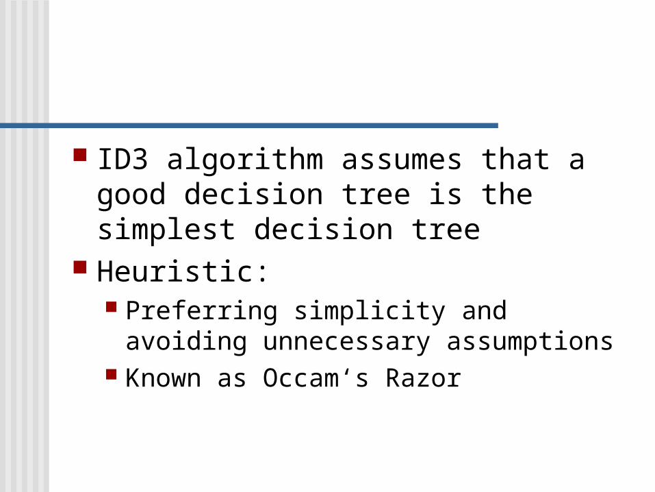
ID3 algorithm assumes that a good decision tree is the simplest decision tree
Heuristic: Preferring simplicity and avoiding
unnecessary assumptions Known as Occam‘s Razor
Occam Razor was first articulated by the medieval logician William of Occam in 1324
• born in the village of Ockham in Surrey (England) about 1285, believed that he died in a convent in Munich in 1349, a victim of the Black Death
• It is vain do with more what can be done with less..
We should always accept the simplest answer that correctly fits our data
The smallest decision tree that correctly classifies all given examples
Zur Anzeige wird der QuickTime™ Dekompressor „TIFF (Unkomprimiert)“ benötigt.

The simplest decision tree that covers all examples should be the least likely to include unnecessary constraints
ID3 selects a property to test at the current node of the tree and uses this test to partition the set of examples
The algorithm then recursively constructs a sub tree for each partition
This continuous until all members of the partition are in the same class
• That class becomes a leaf node of the tree

Because the order of tests is critical to constructing a simple tree, ID3 relies heavily on its criteria for selecting the test at the root of each sub tree

Top-Down Induction of Decision Trees ID3
1. A the “best” decision attribute for next node
2. Assign A as decision attribute (=property) for node
3. For each value of A create new descendant
4. Sort training examples to leaf node according to
the attribute value of the branch5. If all training examples are perfectly
classified (same value of target attribute) stop, else iterate over new leaf nodes

Zur Anzeige wird der QuickTime™ Dekompressor „TIFF (LZW)“
benötigt.

ID3 constructs the tree for credit rist assessment Beginning with the full table of examples, ID3 selects income as the root property using function selecting “best” property (attribute)
The examples are divided, listed by their number in the list
Zur Anzeige wird der QuickTime™ Dekompressor „TIFF (LZW)“
benötigt.

ID3 applies the method recursively for each partition The partition {1,4,7,11} consists entirely of high-risk
individuals, a node is created ID3 selects credit history property as the root of the
subtree for the partition {2,3,12,14} Credit history further divides this partition into {2,3},
{14} and {12} ID3 implements a form of hill climbing in the
space of all possible trees

Zur Anzeige wird der QuickTime™ Dekompressor „TIFF (LZW)“
benötigt.

Hypothesis Space Search ID3two classes: +,-
+ - +
+ - +
A1
- - ++ - +
A2
+ - -
+ - +
A2
-
A4+ -
A2
-
A3- +

Two classes: +,-
Zur Anzeige wird der QuickTime™ Dekompressor „TIFF (LZW)“
benötigt.
Information Theory Information theory (Shannon 1948) provides the
information content of a message We may think of a message as an instance in a
universe of possible messages The act of transmitting a message is the same
as selecting one of these possible messages Define information content of a message as
depending upon both the size of this universe and the frequency with which each possible message occurs

The importance of the number of possible messages is evident in an example from gambling: compare a message correctly predicting the outcome the spin of the roulette wheel with one predicting the outcome of toss of an honest coin
Message concerning roulette is more valuable to us

Shannon formalized these intuitions Given a universe of messages
M={m1,m2,...,mn} and a probability p(mi) for the occurrence of each message, the information content (also called entropy)of a message M is given
€
I(M) = −p(mii=1
n
∑ )log2(p(mi))
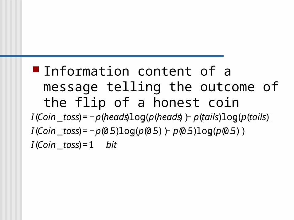
Information content of a message telling the outcome of the flip of a honest coin
€
I(Coin _ toss) = −p(heads)log2(p(heads)) − p(tails)log2(p(tails))
I(Coin _ toss) = −p(0.5)log2(p(0.5)) − p(0.5)log2(p(0.5))
I(Coin _ toss) =1 bit
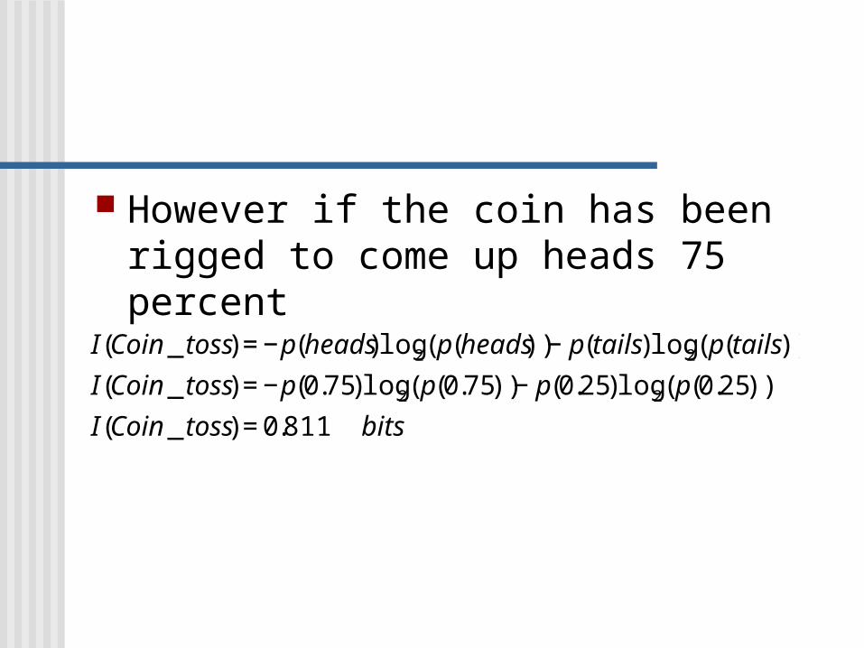
However if the coin has been rigged to come up heads 75 percent
€
I(Coin _ toss) = −p(heads)log2(p(heads)) − p(tails)log2(p(tails))
I(Coin _ toss) = −p(0.75)log2(p(0.75)) − p(0.25)log2(p(0.25))
I(Coin _ toss) = 0.811 bits
We may think of a decision tree as conveying information about the classification of examples in the decision table
The information content of the tree is computed from the probabilities of different classifications
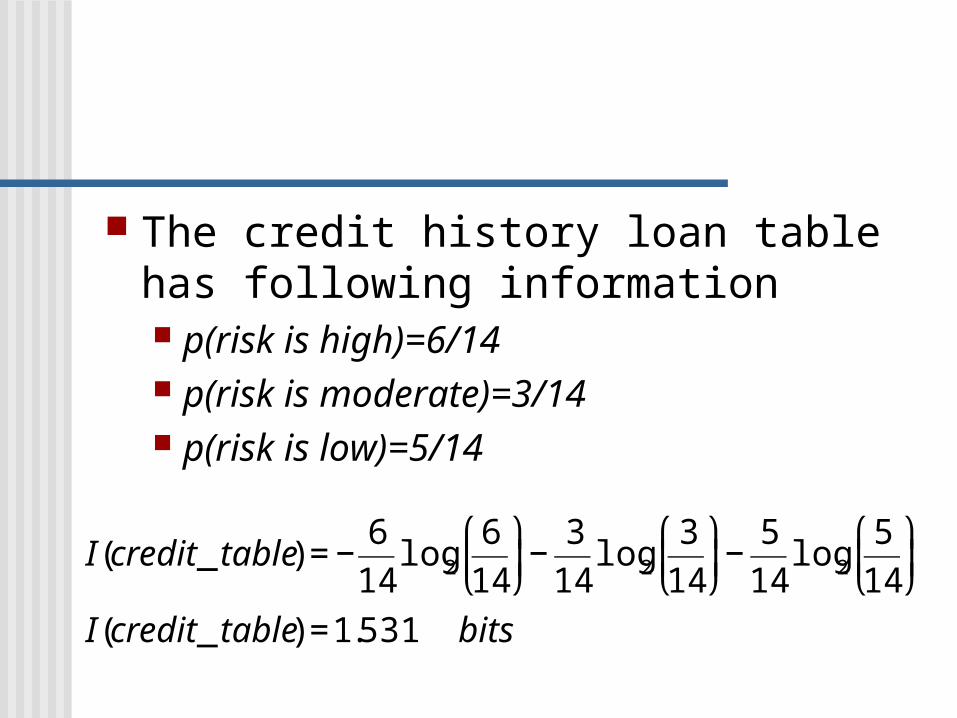
The credit history loan table has following information p(risk is high)=6/14 p(risk is moderate)=3/14 p(risk is low)=5/14
€
I(credit _ table) = −6
14log2
6
14
⎛
⎝ ⎜
⎞
⎠ ⎟−
3
14log2
3
14
⎛
⎝ ⎜
⎞
⎠ ⎟−
5
14log2
5
14
⎛
⎝ ⎜
⎞
⎠ ⎟
I(credit _ table) =1.531 bits

For a given test, the information gain provided by making that test at the root of the current tree is equal to Total information of the table - the amount of
information needed to complete the classification after performing the test
The amount of information needed to complete the tree is defined as weighted average of the information content of each sub tree
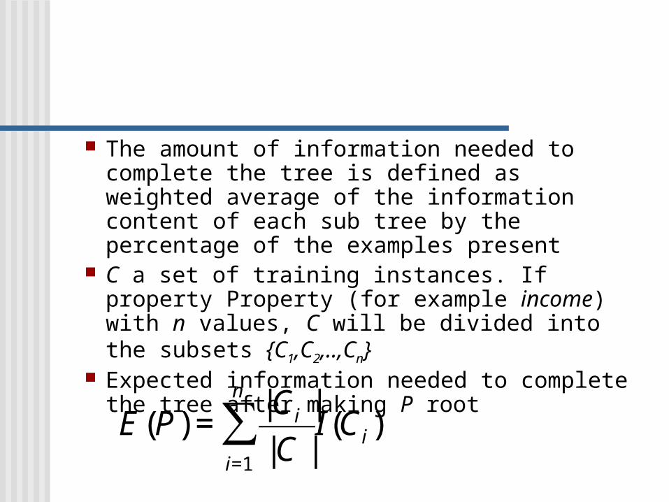
The amount of information needed to complete the tree is defined as weighted average of the information content of each sub tree by the percentage of the examples present
C a set of training instances. If property Property (for example income) with n values, C will be divided into the subsets {C1,C2,..,Cn}
Expected information needed to complete the tree after making P root
€
E(P) =|Ci |
|C |i=1
n
∑ I(Ci)

The gain from the property P is computed by subtracting the expected information to complete E(P) fro the total information€
E(P) =|Ci |
|C |i=1
n
∑ I(Ci)
€
gain(P) = I(C) − E(P)
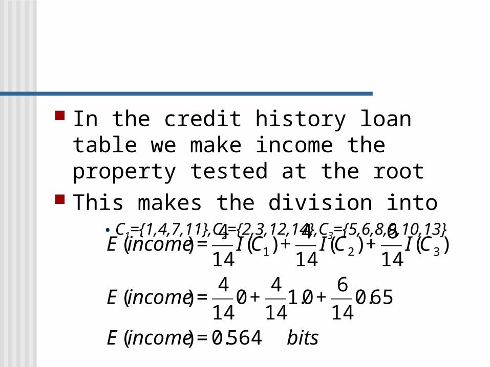
In the credit history loan table we make income the property tested at the root
This makes the division into• C1={1,4,7,11},C2={2,3,12,14},C3={5,6,8,9,10,13}
€
E(income) =4
14I(C1) +
4
14I(C2) +
6
14I(C3)
E(income) =4
140 +
4
141.0 +
6
140.65
E(income) = 0.564 bits
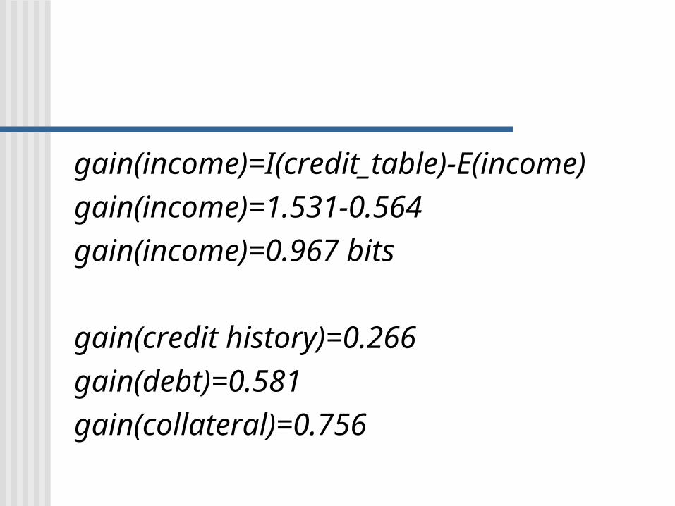
gain(income)=I(credit_table)-E(income)
gain(income)=1.531-0.564
gain(income)=0.967 bits
gain(credit history)=0.266
gain(debt)=0.581
gain(collateral)=0.756
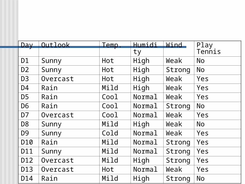
Day Outlook Temp. Humidity Wind Play TennisD1 Sunny Hot High Weak NoD2 Sunny Hot High Strong NoD3 Overcast Hot High Weak YesD4 Rain Mild High Weak YesD5 Rain Cool Normal Weak YesD6 Rain Cool Normal Strong NoD7 Overcast Cool Normal Weak YesD8 Sunny Mild High Weak NoD9 Sunny Cold Normal Weak YesD10 Rain Mild Normal Strong YesD11 Sunny Mild Normal Strong YesD12 Overcast Mild High Strong YesD13 Overcast Hot Normal Weak YesD14 Rain Mild High Strong No

Zur Anzeige wird der QuickTime™ Dekompressor „TIFF (LZW)“
benötigt.

Zur Anzeige wird der QuickTime™ Dekompressor „TIFF (LZW)“
benötigt.

Decision tree examples
ID3 algorithm Occam Razor Top-Down Induction in Decision Trees Information Theory gain from property P
Enhancements to basic decision tree induction
C4.5, CART algorithm


![Decision Trees - Penn Engineering · 2019-01-22 · Basic Algorithm for Top-Down Induction of Decision Trees [ID3, C4.5 by Quinlan] node = root of decision tree Main loop: 1. Aßthe](https://static.documents.pub/doc/80x56/5f5860fa1af89f4c3b659662/decision-trees-penn-engineering-2019-01-22-basic-algorithm-for-top-down-induction.jpg)


