BearWorks BearWorks

MSU Graduate Theses

Spring 2019

Decision Trees and Their Application for Classification and Decision Trees and Their Application for Classification and

Regression Problems Regression Problems

Obinna Chilezie Njoku Missouri State University, Obinna15@live.missouristate.edu

As with any intellectual project, the content and views expressed in this thesis may be

considered objectionable by some readers. However, this student-scholar’s work has been

judged to have academic value by the student’s thesis committee members trained in the

discipline. The content and views expressed in this thesis are those of the student-scholar and

are not endorsed by Missouri State University, its Graduate College, or its employees.

Follow this and additional works at: https://bearworks.missouristate.edu/theses

Part of the Statistical Models Commons

Recommended Citation Recommended Citation Njoku, Obinna Chilezie, "Decision Trees and Their Application for Classification and Regression Problems" (2019). MSU Graduate Theses. 3406. https://bearworks.missouristate.edu/theses/3406

This article or document was made available through BearWorks, the institutional repository of Missouri State University. The work contained in it may be protected by copyright and require permission of the copyright holder for reuse or redistribution. For more information, please contact BearWorks@library.missouristate.edu.

DECISION TREES AND THEIR APPLICATION FOR CLASSIFICATION AND

REGRESSION PROBLEMS

A Master’s Thesis

Presented to

The Graduate College of

Missouri State University

TEMPLATE

In Partial Fulfillment

Of the Requirements for the Degree

Master of Science, Mathematics

By

Obinna Chilezie Njoku

May 2019

ii

DECISION TREES AND THEIR APPLICATION FOR CLASSIFICATION AND

REGRESSION PROBLEMS

Mathematics

Missouri State University, May 2019

Master of Science

Obinna Chilezie Njoku

ABSTRACT

Tree methods are some of the best and most commonly used methods in the field of statistical

learning. They are widely used in classification and regression modeling. This thesis introduces

the concept and focuses more on decision trees such as Classification and Regression Trees

(CART) used for classification and regression predictive modeling problems. We also introduced

some ensemble methods such as bagging, random forest and boosting. These methods were

introduced to improve the performance and accuracy of the models constructed by classification

and regression tree models. This work also provides an in-depth understanding of how the CART

models are constructed, the algorithm behind the construction and also using cost-complexity

approaching in tree pruning for regression trees and classification error rate approach used for

pruning classification trees. We took two real-life examples, which we used to solve

classification problem such as classifying the type of cancer based on tumor type, size and other

parameters present in the dataset and regression problem such as predicting the first year GPA of

a college student based on high school GPA, SAT scores and other parameters present in the

dataset.

KEYWORDS: decision trees, classification trees, regression trees, bagging, random forest,

boosting

iii

DECISION TREES AND THEIR APPLICATION FOR CLASSIFICATION AND

REGRESSION PROBLEMS

By

Obinna Chilezie Njoku

A Master’s Thesis

Submitted to the Graduate College

Of Missouri State University

In Partial Fulfillment of the Requirements

For the Degree of Master of Science, Mathematics

May 2019

Approved:

George Mathew, Ph.D., Thesis Committee Chair

Yingcai Su, Ph.D., Committee Member

Songfeng Zheng, Ph.D., Committee Member

Julie Masterson, Ph.D., Dean, Graduate College

In the interest of academic freedom and the principle of free speech, approval of this thesis

indicates the format is acceptable and meets the academic criteria for the discipline as

determined by the faculty that constitute the thesis committee. The content and views expressed

in this thesis are those of the student-scholar and are not endorsed by Missouri State University,

its Graduate College, or its employees.

iv

TABLE OF CONTENTS

Introduction Page 1

Classification and Regression Trees Page 5

Regression Trees Page 5

Classification Trees Page 10

Bagging, Random Forest and Boosting Page 12

Application of Classification and Regression Tree to Real World

Data

Page 20

Application of Classification Tree to Real World Data Page 20

Application of Regression Tree to Real World Data Page 26

References Page 37

v

LIST OF TABLES

Table 1. Breast tumor biopsy up 1992 (Partial) Page 20

Table 2. Summary of the model for biopsy data Page 22

Table 3. Confusion matrix of the biopsy base model Page 23

Table 4. Confusion matrix of the pruned model for biopsy data Page 26

Table 5. Information of 219 first year student at a college in 1996 Page 27

Table 6. Summary of the model for first year GPA data Page 28

Table 7. Summary of the importance of each variable in the

random forest model

Page 33

vi

LIST OF FIGURES

Figure 1.1 An example of a decision tree Page 3

Figure 2.1 Partitions and classification and regression trees (CART) Page 7

Figure 3.1 Tree structure of the base model for biopsy data Page 23

Figure 3.2 A plot of the cross-validation errors against the size of

terminal nodes and the value of the cost complexity parameter k

Page 24

Figure 3.3 Tree structure of the pruned model for biopsy data Page 25

Figure 3.4 Tree structure of the base model for the first-year GPA Page 29

Figure 3.5 A plot of the cross-validation errors against the size of the

terminal node

Page 30

Figure 3.6 Tree structure of the pruned model for first-year GPA data Page 30

Figure 3.7 Plot of the first-year GPA test data over the predictions from

the base model

Page 31

Figure 3.8 Plot of the first-year GPA test data over the predictions from

the bagging model

Page 32

Figure 3.9 Plot of the importance measure of each variable Page 34

Figure 3.10 Plot of the summary of the boosted tree Page 35

Figure 3.11 Partial dependence plot for HSGPA variable Page 35

Figure 3.12 Partial dependence plot for SATV variable Page 36

1

INTRODUCTION

The Concept of Statistical learning has been in existence since the late 1960’s, but the

theory didn’t receive any recognition until in the 1990s. The theory was only known for

theoretical analysis of the problems of estimation from a given data set before the 90’s. In the

mid 90’s, new learning algorithms were developed and proposed, this changed the face of

statistical learning theory and made the theory not only for theoretical analysis of dataset but also

a tool for creating practical algorithms for estimating multidimensional functions. As seen from

Sidhu and Caffo (2014), statistical learning theory deals with the problem involving estimation

of predictive functions based on data. This has led to successful applications in fields such

as computer vision, speech recognition, bioinformatics, baseball and several other fields. This

work focuses on the various tree based methods for classification and regression. The models

employed by the tree based methods are known for their simplicity and efficiency when dealing

with large datasets. Work on tree based methods can be traced back to Morgan and Sonquist and

their Automatic Interaction Detection (AID) program developed in 1963. However, this field of

research has its major reference from the seminal book on classification and regression trees by

Breiman, Friedman, Olshen and Stone (1984). Some of the models employed by the tree based

methods divide the predictor space into a number of simpler regions which can be summarized

into trees using the set of rules used in splitting the predictor space into the simpler regions, and

these approaches are known as the decision tree methods. This method is instable despite its

various advantages because any small change in the set of training dataset will likely lead to

changes in the tree structure.

2

Decision tree methods are one of the best and mostly used supervised learning algorithm

in prediction of the accuracy of a model, but performs better with ensemble methods. This work

will include bagging, boosting and random forest approaches, these approaches are also known as

the ensemble methods and they utilize more than a single decision tree for predictive purposes. It

combines several decision trees in a bid to produce a better predictive performance. As seen from

Shubham (2018), the main concept behind the ensemble model is that a group of weak learners

come together to form a strong learner thereby increasing the accuracy of the model. In

predicting the target variable using statistical methods or algorithms, we usually will experience

a difference between the predicted value and the actual values and this difference is caused by

variance and bias. However, ensemble methods such as boosting and bagging help to reduce

these errors. The idea behind the algorithms used by ensemble methods will be discussed

extensively in the next chapter.

According to Teli and Kanikar (2015) decision tree method is a technique in statistical

learning that can be applied to both regression and classification problems. The science and

technology behind the review of large and complex datasets in bid to discover valuable patterns

is very important for modeling and knowledge extraction from the data which are available.

Researchers (theoreticians and practitioners) in this field have continually made great progress

and are still making progress in acquiring methods to make the process more efficient, cost-

effective and accurate. Decision trees, were originally implemented in decision theory and

statistics. The benefits of decision tree are in its ability to handle a variety of input data such as

nominal, numeric and textual, its processing of dataset that containing errors and missing values,

and its availability in various packages of data mining and number of platforms.

3

A decision tree is a graphical representation of specific decision situations that are used

when complex branching occurs in a structured decision. Decision trees are used to extract

knowledge by making decision rules from the large amount of available information. A decision

tree classifier has a simple form which can be compactly stored and that efficiently classifies

new data. In this thesis, we investigate different algorithms to classify and predict the data using

decision tree. Figure 1.1 illustrates a working example of decision tree algorithm as seen from

Shikha (2013) publication on decision trees.

Figure 1.1 An example of a decision

The decision tree from the figure above classifies a case of playing tennis in

correspondence to the weather. For instance, if the Outlook is raining and wind is weak the tree

predicts play tennis to be “No”.

4

From the Figure 1, we see that decision trees are classifiers in the form of a tree structure

where each node is either a leaf node, a decision node and a root node.

• Leaf node: This is also known as the terminal node, and it is any node that doesn’t

have a child node. This node specifies the value of the target attribute.

• Decision node: This is a node that has a child node. This node specifies that some

test is to be carried out on an attribute. Also known as the internal node.

• Root node: This is the first node in a tree structure, usually located at the top or

bottom of the tree depending on how the tree is structured. Other nodes in the tree

structure originate from the root node.

In the field of statistical learning today, decision tree techniques are frequently used to

create models that best predict the value of desired input using several inputs. Breiman et al

(1984), came up with the Classification and Regression Trees (CART) methodology as an

umbrella term to refer to the following types of decision trees:

• Classification Trees: where the target variable is categorical and the tree is used to

identify the "class" within which a target variable would likely fall into.

• Regression Trees: where the target variable is continuous and tree is used to predict its

value.

In the subsequent chapters, we will see a breakdown and illustrations of the concept of

CART and other predictive tree algorithms. This work will also utilize some dataset and R

programming language in the other to create a better insight of the subject matter.

5

CLASSIFICATION AND REGRESSION TREES

In the previous chapter, we stated that decision trees are classified into classification and

regression tress which are statistical learning methods used to construct prediction models from

datasets. Loh (2011) claims that the classification and regression tree methods obtain their

models through the recursive partitioning of the datasets and fitting a simple model within each

partition. These partitions can be represented graphically as decision trees.

Regression Trees

Regression tree can be referred to as a variant of decision tree which was developed to

estimate real-valued functions, see Loh (2011). They are designed for dependent variables that

take continuous or ordered discrete values, where the sum of the squared difference between the

predicted and observed values is used to measure the prediction error. The datasets for the

operation of regression trees consists a single output variable with one or more input variables.

The output and input variables are also known as response and predictor variables, respectively,

and the output variable is numerical. Generally, the methodology employed in the construction

of regression trees allows the input variables to be a combination of continuous and categorical

variables. Whenever each decision node in the regression tree contains a test on the values of

some input variables, a decision tree is developed and the terminal node of the tree contains the

values of the predicted output variable.

James, Witten, Hastie and Tibshirani (2013) introduces the process of building a

regression tree as the application of a method known as binary recursive partitioning. Before this

process is applied, we first split the dataset set into two portions, the training set and testing sets.

6

The model is developed and trained using the training set while the testing data set is

used to test the model to view its accuracy in prediction. The binary recursive partitioning

process is an iterative process which splits the dataset into simple partitions and then continues to

split every partition into smaller partitions or groups at each stage of the process.

Let 𝑦1, 𝑦2, … , 𝑦𝑁 be a collection of observation of the response variable 𝑦𝑖. Each observed

value 𝑦𝑖 , 𝑖 = 1, 2, … , 𝑁, depends on the explanatory variable 𝑋1, 𝑋2, … , 𝑋𝑝. This implies that we

divide the predictor space which is the set of possible values for 𝑋1, 𝑋2, … , 𝑋𝑝 into 𝐽- distinct and

non-overlapping regions, 𝑅1, 𝑅2. . . , 𝑅𝑗. Then for every observation that falls into the region Rj,

we make the same prediction, which is simply the mean of the response values for the training

observations in 𝑅𝑗. The regions can have any shape depending on the user. Nevertheless, we can

decide to split the predictor space into j-high-dimensional rectangles or boxes because of the ease

and effortlessness in the interpretation of the resulting predictive model. Then we consider all the

predictors 𝑋1, 𝑋2, … , 𝑋𝑝, and all the possible values of the split for each of the predictors. We

choose the predictor and split point that will result into a tree that has the lowest Residual Sum

Square (RSS).

In essence, the goal is to find boxes 𝑅1, 𝑅2. . . , 𝑅𝑗 that minimizes the Residual Sum Square

which is given by

𝑅𝑆𝑆 = ∑ ∑ (𝑦𝑖 − �̂�𝑅𝑗)2

𝑖∈𝑅𝑗 (2.1)𝐽

𝑗=1

where �̂�𝑅𝑗 is the mean response for the training data set within the 𝑗𝑡ℎ box.

Regrettably, considering each possible partitions of the feature space into J boxes

constitutes a huge challenge computationally. Therefore, we are forced to take a top-down

greedy approach called recursive binary splitting. The process is known as at top-down process

since it starts at the top of the tree, that is, the point where all the observations belong to one

7

region and then splits the predictor space. Each split is specified through two new branches

further down the tree.

From James et al. (2013) we understood that in performing the recursive binary splitting,

we first select a predictor and a split point such that splitting the predictor space into two regions

results to the greatest possible reduction in RSS. This process is repeated, with the aim of finding

the best predictor and best split point in order to split the data further and minimize the RSS

within each of the regions. However, instead of splitting the entire predictor space this time, we

split one of the previously identified regions. This process is continued until a certain criterion is

reached. As shown in Figure 2.1, we was taken from James et al. (2013).

Figure 2.1 Partitions and classification and regression trees (CART)

8

From Figure 2.1, we can see a combination of various partitioning used in CART. Top

left describes a partition of two-dimensional space that could not result from a recursive binary

splitting. Top right shows the output of recursive binary splitting on a two-dimensional space.

While bottom left is a tree corresponding to the partition in the top right panel. The bottom right

represents a perspective plot of the prediction surface corresponding to that tree.

James et al. (2013) claimed that the recursive binary splitting process may produce good

predictions on the training data set but will most likely overfit the data, which yields a poor

performance on the testing data set because the tree produced might be too complicated. A

smaller tree with less split might produce better interpretation and lower variance of the data.

Another alternative to the method above is to construct the tree continuously as long as the

decrease in the RSS ascribable to each split surpasses a threshold, this approach will result into

smaller trees.

Nevertheless, a problem arises since a worthless spilt early on in the tree might be

followed by a very good split later on, that is, a split that leads to a large reduction in RSS later

on. Hence the best approach is called the tree pruning approach. This approach grows a very

large tree 𝑇0 and then prunes it down to acquire a subtree that gives rise to the lowest test error

rate possible. Using the cross-validation approach, we can estimate a given subtree’s test error,

estimating the cross-validation error for every subtree will be too clumsy since there exist a very

large number of subtrees. Hence, we use a cost complexity pruning approach also known as

weakest link pruning method which enables us to select a small set of subtrees for consideration

rather than considering every subtree. Therefore, we consider only the subtrees indexed by a

nonnegative tuning parameter .

9

In this section, we will investigate in detail the algorithm for building a regression tree,

that is, the step by step procedure or set of rules followed in constructing regression trees, as in

James et al. (2013).

i. Use recursive binary splitting to grow a large tree on the training data, stopping only

when each terminal node has fewer than some minimum number of observations.

ii. Apply cost complexity pruning to the large tree in order to obtain a sequence of best

subtrees, as a function of α.

iii. Use K-fold cross-validation to choose α. That is, divide the training observations into K

folds. For each k = 1, . . ., K:

a. Repeat Steps i and ii on all but the kth fold of the training data.

b. Evaluate the mean squared prediction error on the data in the left-out kth fold, as a

function of α. Average the results for each value of α, and pick α to minimize the

average error.

iv. Return the subtree from Step ii that corresponds to the chosen value of α.

James et al (2013), further explained the algorithm by defining some terminology to be

used in the mathematical formula of the algorithm equation;

• |𝑇| indicates the number of terminal nodes of the tree 𝑇.

• 𝑅𝑗 is the rectangle or box corresponding to the 𝑗𝑡ℎ terminal node.

• �̂�𝑅𝑗is the predicted response associated with 𝑅𝑗.

• α controls a trade-off between the subtree’s complexity and its fit to the training data.

For each value of α, there is a corresponding subtree 𝑇 ∈ 𝑇0 such that

∑ ∑ (𝑦𝑖 − �̂�𝑅𝑗)2 + 𝛼|𝑇|

𝑥𝑖∈𝑅𝑛

(2.2)

|𝑇|

𝑛=1

is as small as possible. This is equivalent to constraining the value of |𝑇 |, that is,

min {∑ (𝑦𝑖 – �̂�𝑅𝑗)

2} 𝑠𝑢𝑏𝑗𝑒𝑐𝑡 𝑡𝑜 |𝑇| ≤ 𝑐𝛼

𝑖

.

10

Using Lagrange multipliers, we find that

Δ𝑔 = ∑(𝑦𝑖 − �̂�𝑅𝑗)2 + 𝜆(|𝑇| − 𝑐𝛼)

𝑖

(2.3)

We wish to find this 𝑚𝑖𝑛𝑇,λ,Δ𝑔, which is a discrete optimization problem. However, since

we’re minimizing over T and λ this implies the location of the minimizing T doesn’t depend on

cα. But each cα will imply an optimal value of λ. As far as finding the best tree is concerned, we

might as well, just pick a value of λ, and minimize.

Δ𝑔′ = ∑ (𝑦𝑖 − �̂�𝑅𝑗)2 + 𝜆(|𝑇| )𝑖 (2.4)

If λ = α, then, we get equation (2.2).

According to James et al (2013), when 𝛼 = 0, then the subtree 𝑇 will simply equal 𝑇𝑜,

because equation (2.2) measures the training error. However, as = 0 increases from 0, there is a

price to pay for having a tree with many terminal nodes, and so (2.2) will be minimized for a

smaller sub-tree. As α = 0 increases from 0 in (2.2), branches are pruned from the tree in a nested

and predictable way (resulting in the whole sequence of subtrees as a function of α = 0 is easy).

We can select an α using a validation set of using cross-validation. This process is summarized in

the algorithm earlier.

Classification Trees

James et al. (2013) claims classification trees are very similar to regression trees, only

that classification trees are used to predict a discrete category (qualitative response) rather than a

numeric value (quantitative values). The input variables used for classification can be numerical

or categorical variables. For regression trees, the predicted response for an observation is given

by the mean response of the training observations that belong to the same terminal node.

11

In the case of classification, we predict that each observation belongs to the most

commonly occurring class of training observations in the region to which it belongs to. The

process of building a classification tree is quite similar to that of a regression tree. James et al.

(2013) claims that the recursive binary approach is used in growing the classification tree

likewise regression tree but, in the classification tree setting, the Residual Sum of Square (RSS)

cannot be used as a standard for making splits. A better option to RSS approach is the

classification error rate and this is simply the fraction of the training observations in that region

that do not belong to the most common class. The classification error is given by;

𝐸 = 1 − max �̂�𝑚𝑘 (1)

where �̂�𝑚𝑘 represents the proportion of training observations in the region m that are from class

k.

There are other measures for making splits as can be seen from James et al (2013). These

two measures are Cross entropy and Gini index and are preferred since the classification error is

insufficiently sensitive for tree growth.

The Gini Index, see James et al. (2013) is given by

𝐺 = ∑ �̂�𝑚𝑘(1 − �̂�𝑚𝑘) (2)𝐾𝑘=1

which is a measure of the total variance across k classes, where �̂�𝑚𝑘 represents the proportion of

training observations in the region m that are from class k.

Gini Index is also called a measure of node purity because if all of the values of �̂�𝑚𝑘 , the

proportion of training observations in the region m that are from class k are close to 0 or 1 then

the Gini index has a small value which can be verified from (1). This implies that a node

contains mostly training observations from a single class.

Cross entropy, James et al. (2013) is an alternative to the Gini Index and its given by

12

𝐶 = − ∑ �̂�𝑚𝑘 log(�̂�𝑚𝑘)

𝐾

𝑘=1

(3)

Since;

0 ≤ �̂�𝑚𝑘 ≤ 1

we have

0 ≤ −�̂�𝑚𝑘 log (�̂�𝑚𝑘)

The cross entropy will take a value near 0 if the �̂�𝑚𝑘′𝑠 are all near 0 or 1.

In building a classification tree, we use either Cross entropy or Gini index to evaluate the

quality of a particular split, because these two approaches are more sensitive to node purity than

the classification error rate. However, when pruning the tree any of the three approaches can be

used but the classification error rate is preferable if the prediction accuracy of the final pruned

tree is the goal. In the case of classification trees, the deviance is given by the summary function

and it can be calculated by

−2 ∑ ∑ 𝑛𝑚𝑘 log(�̂�𝑚𝑘)

𝑘𝑚

(4)

𝑛𝑚𝑘 is the number of observations in the 𝑚𝑡ℎ terminal node that belongs to class k.

A tree gives a good fit to the training data if the deviance is small. The residual mean

deviance is simply the deviance divided by 𝑛 − |𝑇0|.

Bagging, Random Forest and Boosting

According to Rokach (2010) bagging, random forest and boosting are machine learning

ensembles designed to improve the accuracy of machine learning algorithms for statistical

classification and regression. They are most commonly applied to decision tree methods as

building blocks in the creation of very powerful predictive models.

13

Bagging. Breiman (1994) in his technical report proposed bagging (bootstrap

aggregation) as a method to enhance classification by combining classifications of randomly

generated training sets. According to Breiman (1996) “bagging leads to improvements for

unstable procedures” which includes classification and regression trees, subset selection in linear

regression and artificial neural networks. His technical report in 1994 featured an interesting

application of the concept of bagging showing improvement in preimage learning. However, in

the case of K-Nearest neighbor’s procedure, bagging can softly reduce the performance of the

method and stable methods like it Breiman (1996). Bagging is also known as bootstrap

aggregation and it’s a special case of the model averaging approach. It also helps to reduce

overfitting of the model.

According to James et al. (2013) the bootstrap approach is simply a fundamental

resampling tool in statistics. The basic idea underlying the bootstrap is that we can estimate the

true 𝐹 by calling the empirical distribution �̂�. Given a set of training data (𝑥𝑖 , 𝑦𝑖), 𝑖 = 1, . . . , 𝑛 is

the empirical distribution function �̂� is simply

𝑃�̂� {(𝑋, 𝑌) = (𝑥, 𝑦)} = {1

𝑛, 𝑖𝑓 (𝑥, 𝑦) = (𝑥𝑖 , 𝑦𝑖) 𝑓𝑜𝑟 𝑠𝑜𝑚𝑒 𝑖

0 𝑜𝑡ℎ𝑒𝑟𝑤𝑖𝑠𝑒

This is just a discrete probability distribution, putting equal weight (1

𝑛) on each of the observed

training points.

According to Hastie, Tibshirani and Friedman (2008) given a set of training observations

𝑊 = {(𝑥1, 𝑦1), (𝑥2, 𝑦2), . . . . , (𝑥𝑛, 𝑦𝑛)} obtaining the predictions at 𝑓(𝑥) at input 𝑥 with variance

𝜎2, the variance of the mean of the set of training observations is given by 𝜎2/𝑛 which implies

that boosting aggregation or bagging averages the prediction over a collection of bootstrap

observations, thereby reducing its variance.

14

However, from the above we can say that a more natural way of reducing the variance

and increase prediction accuracy using bagging is to obtain many training observation sets and

average the resulting predictions. For each bootstrapped training observation 𝑊∗𝑏, 𝑏 =

1, 2, 3, … … … , 𝐵, we fit the model giving prediction 𝑓∗𝑏(𝑥) the bagging estimate is given by

𝑓𝑏𝑎𝑔(𝑥) =1

𝐵∑ 𝑓∗𝑏(𝑥)

𝐵

𝑏=1

We can denote the empirical distribution function putting equal probability 1

𝑛 on each of

the data points (𝑥𝑖 , 𝑦𝑖) by �̂�. Literally the real bagging estimate is given by 𝐸𝑃 ̂𝑓∗(𝑥)

where 𝑊∗ = {(𝑥1∗, 𝑦1

∗), (𝑥2∗ , 𝑦2

∗), . . . . , (𝑥𝑛∗ , 𝑦𝑛

∗)}

and (𝑥𝑖∗, 𝑦𝑖

∗) ~ �̂� 𝑓𝑏𝑎𝑔(𝑥) =1

𝐵∑ 𝑓∗𝑏(𝑥)𝐵

𝑏=1 is a Monte Carlo estimate of the true bagging

estimate, approaching it as B → ∞.

According to James et al. (2013), bagging is very useful for decision trees and can also

improve predictions for regression methods. In order to apply bagging to regression trees, we just

simply build B deep grown trees without pruning them using B bootstrapped training

observations, and we take average of the emerging predictions. Each of the resulting regression

tree will have a large variance but a low bias and when the constructed B trees are averaged, it

will lead to a reduction in the variance. However, applying bagging to a classification problem in

order to predict a qualitative output say Y is more involved and has a few possible approaches.

The most common and simplest approach is by taking majority vote of all the class predicted by

each of the B trees. The class occurring the most in the B predictions is selected as the predicted

class.

15

It appears that every bagged model has a very simple approach of estimating its test error

without the need of carrying out the cross-validation or the validation set approach more details

can be found in James et al. (2013). That method is the known as the Out-of-Bag (OOB) error

estimation which is simply a method of measuring the prediction error of statistical learning

model using bootstrap aggregation to sub-sample data samples used for training. OOB is the

mean prediction error on each training sample 𝑥ᵢ, using only the trees that did not have 𝑥ᵢ in their

bootstrap sample. Recollect that in bagging method, trees are continuously fit to bootstrapped

subset observations. On the average, each bagged tree is obtained from about (2 3⁄ ) of the

observations. The (1 3⁄ ) left is referred to as the Out-of-bag observations, we predict the

response for the 𝑖𝑡ℎ observation with every tree where that observation was OOB. This will give

(𝐵/3) predictions for the 𝑖𝑡ℎ observation, to obtain a single prediction for the 𝑖𝑡ℎ observation,

we take average of the (𝐵/3) observations if it is a regression problem and take majority vote if

it’s a classification problem. Using this approach an OOB prediction can be derived for each on

the n observations and an overall OOB MSE in the case of regression and classification error in

the case of classification can be obtained. The resulting OOB error becomes a valid estimate of

the test error for the bagged models since each error was derived from observations that was not

used to fit the tree.

Random Forest. Breiman (2001) proposed random forest as combinations of tree

predictors in such a way that each tree relies on the value of random vector sampled

independently and has the same distribution for all trees in the forest. Random forest is also a

notable improvement of bagging and it constructs a large collection of de-correlated trees, and

then averages them. On many problems, the performance of random forests is very similar to

boosting, and they are simpler to train and tune. As a consequence, random forests are popular,

16

and are implemented in a variety of packages. As the number of trees in the forest becomes

larger, the generalization error for forest converges to a limit, the generalization error of a forest

of tree classifiers depends on the strength of the individual trees in the forest and the correlation

between them. Breiman (2001) defined random forest simply as a classifier consisting of a

collection of tree-structured classifiers {h(x, Θn), n = 1,2, 3, . . . } where {Θn}, are independent

identically distributed random vectors and each tree casts a unit vote for the most popular class at

input x.

According to Hastie et al. (2008) here are step by step process of applying random forest

to classification or regression trees;

1. For b = 1,2, 3, …, B

(a) Draw a bootstrap sample 𝑊∗ = {(𝑥1∗, 𝑦1

∗), (𝑥2∗ , 𝑦2

∗), . . . . , (𝑥𝑛∗ , 𝑦𝑛

∗)} of size

n from the training data.

(b) Grow a random-forest tree 𝑇𝑏 to the bootstrapped data, by recursively

repeating the following steps for each terminal node of the tree, until the

minimum node size 𝑛𝑚𝑖𝑛 is reached.

i. Select 𝑚 variables at random from the 𝑝 variables.

ii. Pick the best variable or split-point among the 𝑚.

iii. Split the node into two daughter nodes.

2. Output the ensemble of trees {𝑇𝑏}1𝐵

To make a prediction at a new point x:

For Regression: 𝑓𝑟𝑓𝐵 (𝑥) =

1

𝐵∑ 𝑇𝑏(𝑥)𝐵

𝑏=1

For Classification: Let �̂�𝑏(𝑥) be the class prediction of the 𝑏𝑡ℎ random-forest tree.

Then �̂�𝑟𝑓𝐵 (𝑥) = 𝑚𝑎𝑗𝑜𝑟𝑖𝑡𝑦 𝑣𝑜𝑡𝑒 {�̂�𝑏(𝑥)}1

𝐵

According to Hastie et al. (2008) when constructing a tree using a bootstrapped dataset,

before each split it’s best to select 𝑚 ≤ 𝑝 of the input variables randomly to be used for splitting.

A common choice for 𝑚 𝑖𝑠 √𝑝 or even as low as 1. After 𝐵 such trees {𝑇 (𝑥; 𝛩𝑏 )}1𝐵

are grown,

17

the random forest (regression) predictor is

𝑓 𝑟𝑓𝐵 (𝑥) =

1

𝐵∑ 𝑇

𝐵

𝑏=1

(𝑥; 𝛩𝑏)

where Θ𝑏 is the b𝑡ℎ random forest tree in terms of split variables, cut-points at each node,

and terminal-node values. Consequently, reducing 𝑚 will decrease the correlation between any

pair of trees in the ensemble, and hence by decrease the variance of the average. In previous

paragraphs, we have been able to highlight the difference between random forest for

classification and regression.

However, when used for regression random forest averages the predictions from each tree

at a target point𝑥. When used for classification, random forest gets a class vote from each tree

and then classifies using majority votes.

Additionally, James et al. (2013) recommends that;

i. For classification, the default value for 𝑚 𝑖𝑠 √𝑝 and the minimum node size is one.

ii. For regression, the default value for 𝑚 𝑖𝑠 𝑝/3 and the minimum node size is five.

Practically, the best values for these parameters should solely depend on the specific

problem, and the parameters should be treated as tuning parameters.

Random forest uses the Out-of-bag (OOB) samples for the estimation of classification

and prediction errors. An important feature of random forest is that it doesn’t require cross-

validation or a different kind of test set to obtain an unbiased estimate of the test set error.

Random forest estimates internally while processing, and each tree is built with a separate

bootstrap sample and about (1/3) of the observations are left out in the construction of the 𝑖𝑡ℎ

tree. The portion of observations left out are called the out-of-bag samples. Each observation left

18

out in the construction of the 𝑖𝑡ℎtree used to obtain a classification. Therefore, in about (1/3) of

the tree a test set classification is obtained for each observation. Once the process of construction

is completed, let 𝑘 be the class that got most of the votes every time for 𝑚 out of bag samples.

The OOB error estimate is the average of all the cases where the 𝑘 does not equal the true class

of 𝑚. Over time, this process has been proven to be unbiased in many tests.

Boosting. According to James et al. (2013) boosting is similar to the bagging method, it

is another approach used to improve the predictions from decision trees (classification &

regression trees).

However, boosting is a general method that can be applied to many other statistical

learning concepts with the sole aim of improving results of predictions. We will be limiting the

discussion of boosting in this chapter to its application with decision trees. In boosting the trees

are grown sequentially and each tree is grown with data from previously grown tree. It has been

observed by James et al. (2013) that boosting doesn’t use bootstrap samples like bagging, each

tree is fit on a modified version of the original data set. In applying boosting approach to

classification trees, we adopt similar method to that of regression tree. However, for

classification tree it is more involved and there are three major tuning parameters;

i. The number of trees 𝐵. Unlike other statistical learning ensembles (Random forest and

bagging), if 𝐵 is too large boosting can overfit. However, overfitting tends to occur

slowly if at all it occurs. We use cross-validation to select 𝐵.

ii. A small positive number known as the shrinkage parameter (λ). This controls boosting’s

learning rate. The common values are 0.01 or 0.001, and the right choice depends on the

problem. In order to achieve a good performance, a very small λ can require using a very

large value of 𝐵.

iii. The number 𝑑 of splits in each tree, controls the difficulty of the boosted ensemble.

Oftentimes 𝑑 = 1 works perfectly, making each tree a stump, consisting of a single split.

However, the boosted ensemble is fitting an additive model, since each term involves

only a single variable. Generally, the number of splits in each tree (𝑑) is the interaction

depth, and controls.

19

According to James et al. (2013) here are the step by step procedure of applying boosting

to regression trees.

1. Set 𝑓(𝑥) = 0 and 𝑟𝑖 = 𝑦𝑖 for all 𝑖 in the training set.

2. For 𝑏 = 1,2, . . . , 𝐵, repeat:

a) Fit a tree 𝑓𝑏 with 𝑑 splits (𝑑 + 1 terminal nodes) to the training data (𝑋, 𝑟).

b) Update 𝑓 by adding in a shrunken version of the new tree:

𝑓(𝑥) ⟵ 𝑓(𝑥) + 𝜆𝑓𝑏(𝑥)

c) Update the residuals,

𝑟𝑖 ⟵ 𝑟𝑖 − 𝜆𝑓𝑏(𝑥𝑖)

3. Output the boost model

𝑓(𝑥) = ∑ 𝜆𝑓𝑏(𝑥)

𝐵

𝑏=1

The main idea behind this process is that boosting method learns slowly unlike bagging

and random forest which fits a single large decision tree to the data and has a possibility of

overfitting. From the current model, a decision tree is fitted to the residuals from the model. That

is, we fit a tree using the current residuals as the response. Then the new decision tree is included

into the fitted function in order to update the residuals. Each of these trees can be rather small,

with just a few terminal nodes, determined by the parameter 𝑑 in the algorithm. We slowly

improve �̂� in areas of poor performance by fitting smaller trees to the residuals. The shrinkage

parameter λ slows the process furthermore, allowing more and different shaped trees to strike the

residuals. Generally, statistical learning methods that learn slowly tend to perform well.

20

APPLICATION OF CLASSIFICATION AND REGRESSION TREE TO REAL WORLD

DATA

This chapter will discuss the application of the techniques of classification and regression

trees to solve real world classification and regression problems. Our goal is to find the best

model used to obtain the target data from the datasets.

Application of Classification Tree to Real World Data

The data “biopsy” used for building a classification tree is a breast cancer data which was

obtained from the University of Wisconsin Hospitals, Madison from Dr. William H. Wolberg.

This data is available at https://vincentarelbundock.github.io/Rdatasets/datasets.html. It contains

biopsies of breast tumors for 699 patients up to 15 July 1992; scored on a scale of 1 to 10, and

the outcome is also known as shown on Table 1. There are 699 rows and 11 columns.

Table 1. Breast tumor biopsy up 1992 (partial)

Observations ID V1 V2 V3 V4 V5 V6 V7 V8 V9 Class

1 1000025 5 1 1 1 2 1 3 1 1 benign

2 1002945 5 4 4 5 7 10 3 2 1 benign

3 1015425 3 1 1 1 2 2 3 1 1 benign

4 1016277 6 8 8 1 3 4 3 7 1 benign

5 1017023 4 1 1 3 2 1 3 1 1 benign

6 1017122 8 10 10 8 7 10 9 7 1 malignant

7 1018099 1 1 1 1 2 10 3 1 1 benign

8 1018561 2 1 2 1 2 1 3 1 1 benign

9 1033078 2 1 1 1 2 1 1 1 5 benign

21

From Table 1, we define the columns mentioned in the data frame as:

ID: sample code number (not unique)

V1: clump thickness.

V2: uniformity of cell size.

V3: uniformity of cell shape.

V4: marginal adhesion.

V5: single epithelial cell size.

V6: bare nuclei (16 values are missing).

V7: bland chromatin.

V8: normal nucleoli.

V9: mitoses.

Class: "benign" or "malignant".

We are using the ‘tree’ method alongside with other methods from the R package to help

us construct classification models and predict. We are going to separate our dataset into training

and testing data. Since our task is to build a classification trees, we now use the tree () function

on the total dataset to fit a classification tree model to predict the class of tumors using all the

variables. We then obtain the list of variables that were used as internal nodes, terminal nodes

and the misclassification error rate using the summary function.

From the summary table (Table 2) below, we see that the misclassification error rate is

3%. The Residual mean deviance is given by

−2 ∑ ∑ 𝑛𝑚𝑘𝑙𝑜𝑔�̂�𝑚𝑘

𝑘𝑚

𝑛𝑚𝑘 represents the number of observations in the 𝑚𝑡ℎ terminal node that belongs to the

𝑘𝑡ℎ class.

22

Table 2. Summary of the base model for biopsy data

Classification tree:

tree (formula = class~., data = biopsy)

Variables actually used in tree construction: "V2" "V6" "V5" "V1" "V8"

Number of terminal nodes: 9

Residual mean deviance: 0.1603 = 108 / 674

Misclassification error rate: 0.03221 = 22 / 683

The residual mean deviance recorded is the deviance divided by 𝑛 − |𝑇0| and a small

deviance shows that the tree constructed provides a good fit to the training data sets. Plotting the

tree structure constructed, we have the figure below.

For us to properly evaluate the performance of the tree constructed as shown in Figure

3.1, we have to estimate the test error. Hereby splitting the observations into training and testing

data sets and then building the tree with the training set while we evaluate the performance using

the test data. In order to visualize our accuracy, we construct the confusion matrix as shown in

Table 3 below. The confusion matrix in Table 3 shows the true positive, true negative, false

positive and false negative predictions of the base model using the test data sets. We then

calculate the accuracy of the model by dividing the sum of true positives and true negative by n.

After performing cross-validation using the cost complexity, we discover that the trees with 6

and 4 terminal nodes results in the lowest cross-validation error rate with an error of 17. Hence,

we plot the error rate function of both size and k as seen in Figure 3.2.

23

Figure 3.1 Tree structure of the base model for biopsy data

From Table 3 below, we can see that this approach yields an accuracy of about 95.31%.

Next, we consider whether pruning the tree will lead to an improved accuracy of the model by

performing cross-validation to determine optimal level of tree complexity.

Table 3. Confusion matrix for the biopsy base model

n = 299 Predicted: No Predicted: Yes

Actual: No 203 4

Actual: Yes 10 82

We now prune the tree in Figure 3.1 above using the prune mis-class function in R to

obtain a 6-terminal node tree which has the lowest cross-validation error rate. Figure 3.3 shows a

pruned version of the tree constructed earlier. The pruning processes has produced a more

interpretable tree but might not necessarily improve the model. Then we predicted results using

24

our testing data set on the constructed model. In other for us to determine the performance of the

model, we also constructed the confusion matrix as seen below.

The pruning processes has produced a more interpretable tree as seen in Figure 3.3 but

might not necessarily improve the model. Then we predicted results using our testing data set on

the constructed model. In other for us to determine the performance of the model, we also

constructed the confusion matrix as shown in Table 4 below. Table 4, depicts the number of true

positive, true negative, false positive and true positive predicted by the model based on the

testing data set. With the predictions obtained, we proceed to calculate the accuracy as described

below.

Figure 3.2 A plot of the cross-validation errors against the size of terminal nodes and the value of

the cost complexity parameter k.

2 4 6 8 10

20

40

60

80

10

012

014

01

60

cv.biopsy$size

cv.b

iop

sy$

de

v

0 20 40 60 80 100 120

20

40

60

80

10

012

014

01

60

cv.biopsy$k

cv.b

iop

sy$

de

v

25

From Table 4, we can calculate the accuracy of the model by dividing the sum of true

positives and true negative by n. This approach yields an accuracy of about 95%, which didn’t

result in an improvement of the model since the previous model had about the same accuracy.

However, this approach produced a more interpretable tree structure as seen in Figure 3.3. We

can now clearly explain the tree structure constructed by the model, for instance, if uniformity

cell size and bare nuclei is less than 2.5 then the model predicts benign. i.e. V2 < 2.5 and V6 <

2.5 yields benign.

Table 4 above, which depicts the confusion matrix of the pruned model and contains the

true positive, true negative, false positive and false negative predictions of the pruned model

using the test data sets. We then calculate the accuracy of the model by dividing the sum of true

positives and true negative by n.

Figure 3.3 Tree structure of the pruned model for biopsy data

|V2 < 2.5

V6 < 2.5

V1 < 3.5

V2 < 3.5

V6 < 1.5benignbenign malignant

benign malignant

malignant

26

Table 4. Confusion matrix of the pruned model for biopsy data

n = 299 Predicted: No Predicted: Yes

Actual: No 203 4

Actual: Yes 10 82

Application of Regression Tree to Real World Data

In this section, we make use of the data “FirstYearGPA”, which is available from

https://vincentarelbundock.github.io/Rdatasets/datasets.html. The dataset which contains

information from a sample of 219 first year students at a Midwestern college, a sample from a

larger set of data collected in 1996 by a professor at this college. Our goal is to predict their first

year GPA. Table 5 below, depicts a partial representation of the total data sets for the captured

information of first year students.

Table 5 depicts a data frame with 219 observations on the following 10 variables. We

define the columns mentioned in the data frame as:

GPA: First-year college GPA on a 0.0 to 4.0 scale

HSGPA: High school GPA on a 0.0 to 4.0 scale

SATV: Verbal/critical reading SAT score

SATM: Math SAT score

Male: 1= male, 0= female

HU: Number of credit hours earned in humanities courses in high school

SS: Number of credit hours earned in social science courses in high school

FirstGen: 1=student is the first in her or his family to attend college, 0=otherwise

White: 1= white students, 0= others

CollegeBound: 1= attended a high school where >=50% students intended to go on to

college, 0 = otherwise.

27

Table 5. Information of 219 first year at a college collected in 1996 (partial)

GPA HSGPA SATV SATM Male HU SS FirstGen White CollegeBound

3.06 3.83 680 770 1 3 9 1 1 1

4.15 4 740 720 0 9 3 0 1 1

3.41 3.7 640 570 0 16 13 0 0 1

3.21 3.51 740 700 0 22 0 0 1 1

3.48 3.83 610 610 0 30.5 1.5 0 1 1

2.95 3.25 600 570 0 18 3 0 1 1

3.6 3.79 710 630 0 5 19 0 1 1

2.87 3.6 390 570 0 10 0 0 0 0

3.67 3.36 630 560 0 8.5 15.5 0 1 1

3.49 3.7 680 670 0 16 12 0 1 1

3.25 3.53 380 470 0 18 7 0 0 1

3.18 3.48 630 670 0 26.5 1.5 0 0 1

3.85 3.81 680 740 1 34 0 0 1 1

2.58 3.38 710 750 1 8 3 0 1 1

3.5 3.8 670 650 0 20 3 0 1 1

We are using the ‘tree’ method alongside with other methods from the R package to help

in the construction of the regression models and predictions. Here we fit a regression tree to the

dataset. First, we create a training set, and fit the tree to the training data. We now use the tree ()

function on the total dataset to fit a regression tree model to predict the GPA of students using all

the variables. We then obtain the list of variables that were used as internal nodes and terminal

nodes using the summary function. From Table 6 which shows the summary of the base model,

we see that only five of the variables have been used in the construction of the tree. The residual

28

mean deviance in this case, is simply the sum of squared errors for the tree. Plotting the tree

structure constructed, we have the figure below.

Table 6. Summary of the model for first year GPA data

Regression tree:

tree (formula = GPA ~ ., data = FirstYearGPA, subset = train)

Variables actually used in tree construction: "HSGPA" "SATV" "HU" "Male” “SATM"

Number of terminal nodes: 12

Residual mean deviance: 0.08679 = 8.418 / 97

From Table 6 which shows the summary of the base model, we see that only five of the

variables have been used in the construction of the tree. The residual mean deviance in this case,

is simply the sum of squared errors for the tree. We then plot the tree structure constructed by the

model, to obtain Figure 3.4.

The tree structure of the base model as seen in Figure 3.4 predicts a GPA of 2.160 for

students whose HSGPA < 2.835 and SATV < 515 where the variable HSGPA measures the

students High School GPA and SATV measures the Verbal SAT scores. We then consider if

pruning the tree will lead to an improvement of the model by performing a cross-validation.

After performing cross-validation we discover that the tree with 7 terminal nodes results in the

lowest cross-validation error rate. Hence, we plot the error rate as a function of size. Figure 3.5

depicts this plot and in this case, the most complex tree by cross-validation is selected and we

make use of the prune tree method in R to prune the tree obtained by the base model if we wish

to. Pruning the tree helps with solving interpretation problems as we obtain a clearer tree that is

easier to interpret as shown in Figure 3.6 below.

29

Figure 3.4 Tree structure of the base model for first-year GPA data

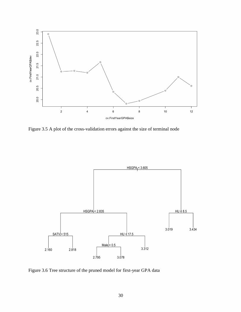
Figure 3.6 below, presents a clearer version of the tree structure of the base model with

fewer terminal nodes making interpretation of the structure easier. For instance, the tree structure

of the base model predicts a 2.160 GPA for students whose HSGPA < 3.605 and SATV < 515.

In keeping with the cross-validation results, we then use the unpruned tree to make

predictions on the test dataset and plot the predictions over the test data as shown below in

Figure 3.7. Figure 3.7 below depicts a plot of the prediction obtained from the pruned model

over the response variable in the test data set. From the predictions obtained as shown in Figure

3.7, we then calculate the test set Mean squared error (MSE) by squaring the mean of the

difference between predicted points and predictor points in the test data set. The MSE helps us to

identify the model which is performing better. We usually prefer models with lower MSE

because it implies that the variation between the predicted value and original value is minimal.

30

Figure 3.5 A plot of the cross-validation errors against the size of terminal node

Figure 3.6 Tree structure of the pruned model for first-year GPA data

31

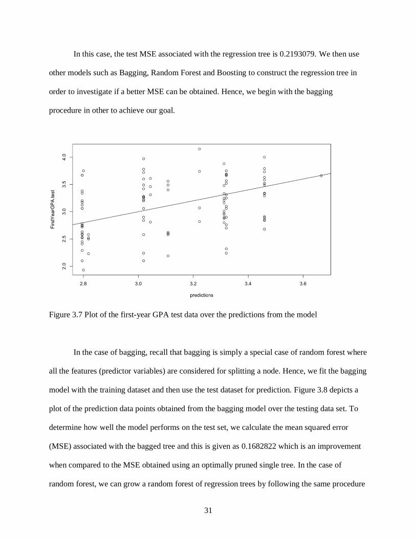
In this case, the test MSE associated with the regression tree is 0.2193079. We then use

other models such as Bagging, Random Forest and Boosting to construct the regression tree in

order to investigate if a better MSE can be obtained. Hence, we begin with the bagging

procedure in other to achieve our goal.

Figure 3.7 Plot of the first-year GPA test data over the predictions from the model

In the case of bagging, recall that bagging is simply a special case of random forest where

all the features (predictor variables) are considered for splitting a node. Hence, we fit the bagging

model with the training dataset and then use the test dataset for prediction. Figure 3.8 depicts a

plot of the prediction data points obtained from the bagging model over the testing data set. To

determine how well the model performs on the test set, we calculate the mean squared error

(MSE) associated with the bagged tree and this is given as 0.1682822 which is an improvement

when compared to the MSE obtained using an optimally pruned single tree. In the case of

random forest, we can grow a random forest of regression trees by following the same procedure

32

as that of bagging except that we don’t use all the predictor variables. In random forest

procedure, the number of predictor variables to be used in building the model can be selected by

the user or by default.

Figure 3.8 Plot of the test data over the predictions from the bagging model

By default, random forest method in R uses 𝑝

3 when building a random forest of

regression trees, where 𝑝 is the number of predictor variables and √𝑝 when building random

forest of classification trees. The calculated value of the mean squared error (MSE) associated

with the random forest tree and this is given as 0.1737903. This indicates that in this case,

bagging yields a better performance than random forest and a single pruned tree.

Table 7 consist of all the predictor variables and their importance in the construction of

the tree structure. Two measures of variable importance are reported in this case, the first

measures the mean decrease of accuracy in predictions on the out of bag samples when a given

33

variable is excluded from the model, while the second measures the total decrease in node

impurity that results from splits over that variable, averaged over all trees as shown by Table 7

below. These measures assist in helping us to make decision of what the key predictors of the

model are.

Table 7. Summary of the Importance of Each Variable in the Random Forest Model

Variable %IncMSE IncNodePurity

HSGPA 19.66344709 5.9598267

SATV 10.50733701 3.7062134

SATM 1.26831957 2.32553

Male 3.87413135 0.4391962

HU 14.71841457 4.2273432

SS 0.03233334 1.4789888

FirstGen 0.06258386 0.048022

White 6.62228033 0.8293439

CollegeBound 2.3176541 0.2203012

As seen from Figure 3.9 below, the two most important variables across all the tree

considered in the random forest are High School GPA (HSGPA) and Number of credit hours

earned in humanities courses in high school (HU). Then, we use the gbm () package in R to fit

boosted regression trees to the FirstYearGPA data set. The summary of the model created

outputs the variables in other of their importance as seen in Figure 3.10 below. We can now

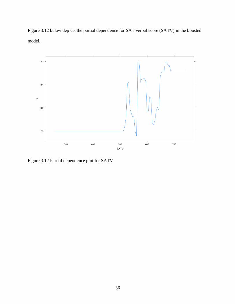
produce a partial dependence plot for the two most important variables. As seen in Figure 3.11

and Figure 3.12 below, these plots show the marginal effect of the selected variables on the

response after integrating out the other variables. In this case, as we might expect, GPA of first

34

year college students are increasing as HSGPA and SATV is increasing. We then used the

boosted model to predict the GPA on the test set. We obtained the value of MSE to be 0.2136224

which is similar to test MSE for the base model but inferior to that of bagging and random forest.

Figure 3.9 Plot of the importance measures of each variable

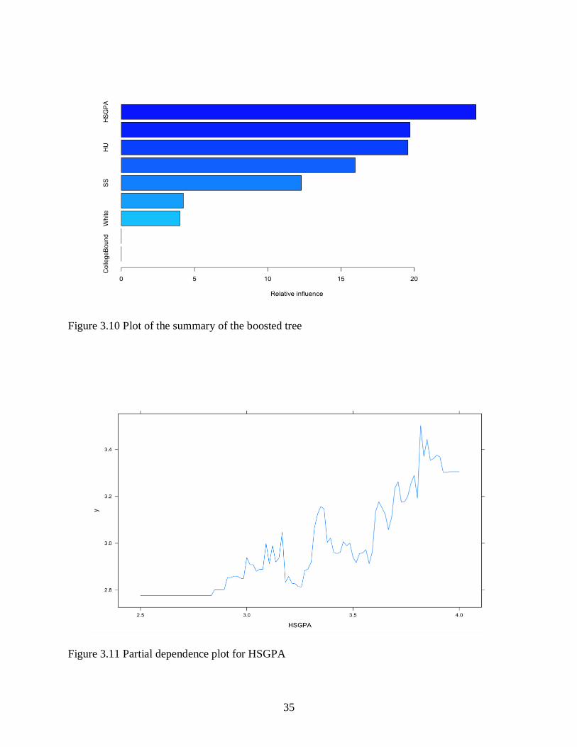
As stated earlier, Figure 3.10 below depicts the summary of the boosted model for the

data set which contains the various predictor variables used in constructing the boosting model

and the relative influence of each the of variables.

On the other hand, Figure 3.11 depicts the partial dependence of the most important

variable which is HSPGA.

35

Figure 3.10 Plot of the summary of the boosted tree

Figure 3.11 Partial dependence plot for HSGPA

36

Figure 3.12 below depicts the partial dependence for SAT verbal score (SATV) in the boosted

model.

Figure 3.12 Partial dependence plot for SATV

37

REFERENCES

Breiman, L. (1994). Heuristics of instability in model selection. Annals of Applied Statistics

Breiman, L (1996). Bagging. Machine Learning. 45 (1): 5 – 32

Breiman, L (2001). Random forests. Machine Learning. 45 (1): 123 – 140

Breiman, L., J. Friedman, R. Olshen, R., and Stone, C. (1984). Classification and regression trees.

Wadsworth Books, 358.

Hastie, T., Tibshirani, R., and Friedman, J. (2008). The elements of statistical learning (2nd

edition). New York: Springer. 587-596

James, G., Witten, D., Hastie, T., and Tibshirani, R. (2013). An introduction to statistical learning.

New York: Springer. 303-332

Loh, W. (2011). Classification and regression trees. WIREs Data Mining Knowledge Discovery

Rokach, L. (2010). Ensemble-based classifiers. Artificial intelligence review. 1-39.

Teli, S., Kanikar, P. (2015). A survey on decision tree based approaches in data mining.

International Journal of Advanced Researches in Computer Science and Software

Engineering, Volume 5, Issue 4. 613.

Shikha, C. (2013). Survey paper on improved methods of ID3 decision tree classification.

International Journal of Scientific and Research Publications 1-4.

Shubham, J. (2018). Reprinted from https://becominghuman.ai/ensemble-learning-bagging-and-

boosting-d20f38be9b1e

Sidhu, G., Caffo, B. (2014). Exploiting pitcher decision-making using reinforcement

learning. Annals of Applied Statistics.