DECLARATION OF THESIS ... -...

DECLARATION OF THESIS / UNDERGRADUATE PROJECT REPORT AND COPYRIGHT

Author’s full name : Mohammed Ameen Abbas AL-Zuraiqi

Date of Birth : 01/01/1989

Title : Modeling and controller design of an industrial pneumatic actuator

system

Academic Session : 2013/2014

I declare that this thesis is classified as:

CONFIDENTIAL (Contains confidential information under the Official Secret Act

1972)*

RESTRICTED (Contains restricted information as specified by the

organization where research was done)*

OPEN ACCESS I agree that my thesis to be published as online open access

(full text)

I acknowledged that Universiti Teknologi Malaysia reserves the right as follows:

1. The thesis is the property of Universiti Teknologi Malaysia

2. The Library of Universiti Teknologi Malaysia has the right to make copies for the

purpose of research only.

3. The Library has the right to make copies of the thesis for academic exchange.

Certified by:

SIGNATURE SIGNATURE OF SUPERVISOR

(NEW IC NO/PASSPORT) NAME OF SUPERVISOR

Date: JULY 2014 Date: JULY 2014

PSZ 19:16 (Pind. 1/07)

NOTES: * If the thesis is CONFIDENTAL or RESTRICTED, please attach with the letter from

the organization with period and reasons for confidentiality or restriction.

UNIVERSITI TEKNOLOGI MALAYSIA

متلب سایت

MatlabSite.com

MatlabSite.com متلب سایت

ii

I declare that I have read this thesis and in my opinion this thesis is sufficient

in terms of scope and quality for the award of the degree of “Bachelor of

Engineering (Electrical - Control and Instrumentation)"

Signature: . . . . . . . . . . . . . . . . . . . . . . . . . . . . . . . . . . . .

Name of Supervisor: Professor Dr Mohd Fua’ad Rahmat.

Date: . . . . . . . . . . . . . . . . . . . . . . . . . . . . . . . . . . . . . . . . . .

متلب سایت

MatlabSite.com


iii

MODELING AND CONTROLLER DESIGN OF AN INDUSTRIAL PNEUMATIC

ACTUATOR SYSTEM

MOHAMMED AMEEN ABBAS AL-ZURAIQI

A project report submitted in partial fulfillment of the requirements for the award of

the degree of Bachelor of Engineering (Electrical - Control and Instrumentation)

Faculty of Electrical Engineering

Universiti Teknologi Malaysia

JULY 2014

متلب سایت

MatlabSite.com


ii

I declare that this thesis entitled “Modeling and controller design of an industrial

pneumatic actuator system” is the result of my own research except as cited in the

references. The thesis has not been accepted for any degree and is not concurrently

submitted in candidature of any other degree.

Signature : ....................................................

Name : MOHAMMED AMEEN ABBAS AL-ZURAIQI

Date : July 2014

متلب سایت

MatlabSite.com


iii

Specially dedicated to my parents

I really miss both of you.

And also to all my family members

متلب سایت

MatlabSite.com


iv

ACKNOWLEDGEMENT

Writing this thesis is a long and difficult journey that requires patients and

dedication. During the entire project, I am glad to receive tons of support from my

family and friends that I really appreciate. The journey would have become harder

and lonely if without their help and encouragement. Second and foremost, I wish to

express my sincere appreciation to my supervisor, Prof Dr Mohd Fua’ad bin Rahmat,

for encouragement, guidance and help.

Besides, I would like to thank my parents and family members for their

support and understanding. Then, I would like to thank my friends who never give

up on me. Thanks to all for continuous support and motivation. I wouldn’t have been

able to complete my project without guidance and consultancy from you all. Thanks

to you all.

متلب سایت

MatlabSite.com


v

ABSTRACT

A pneumatic actuator is a mechanical device which converts the compressed

air energy into mechanical motion. The motion can be rotary or linear, depending on

the type of actuator. Many industries nowadays use pneumatic actuators in

positioning, clamping, gripping, drilling, and conveying operations in the process of

manufacturing and automation. This is due to the advantages pneumatic actuators

offer over other types of force actuators such as electromechanical and hydraulic

actuators. Although pneumatic actuators have many good attributes, achieving

precise and high-speed control of their systems is a challenge. This difficulty is due

to the high-order, time-variant actuator dynamics, and system nonlinearities like air

compressibility, static and coulomb friction, and pressure supply variations. This

project presents the process of modeling a pneumatic actuator system followed by

designing controllers to improve the system performance. To model the system input

and output data are collected from the pneumatic actuator plant using Simulink file.

System Identification Toolbox is used in order to estimate the mathematical model.

Two model structures are selected which are Auto Regressive Exogenous (ARX) and

Auto Regressive Moving Average Exogenous (ARMAX). Model estimation and

validation are done by analyzing residual correlation and best fit percentage. To

improve the system performance conventional PID and Self tuning fuzzy-PID

controllers are designed. The coefficients of the PID controller are tuned using trial

and error method and Ziegler- Nichols method. The system response of the

pneumatic system is improved significantly when applying conversional PID and

self-tuning Fuzzy-PID controllers. Self-tuning fuzzy-PID controller outperformed

the conversional PID controller with 2.22% overshoot only and faster response.

متلب سایت

MatlabSite.com


vi

ABSTRAK

Penggerak pneumatik adalah satu alat mekanikal yang menukarkan tenaga

udara termampat kepada gerakan mekanikal. Ia boleh menjadi sama ada gerakan

putaran atau gerakan linear, bergantung kepada jenis penggerak yang digunakan.

penggerak pneumatik banyak digunakan dalam industri pada hari ini untuk meletak,

pengapit, menggenggam, penggerudian, dan operasi penghantaran dalam proses

pembuatan dan automasi. Hal ini disebabkan oleh kelebihan penggerak pneumatik

yang menawarkan kelebihan berbanding penggerak jenis lain seperti penggerak

elektromekanik dan hidraulik. Walaupun penggerak pneumatik mempunyai banyak

sifat-sifat yang baik, untuk mencapai kawalan yang tepat dalam kelajuan yang tinggi

didalam sistem mereka merupakan suatu cabaran. Kesukaran ini adalah disebabkan

oleh susunan tinggi, kebergantungan pada masa ciri dinamik penggerak dinamik, dan

sistem yang tidak linear seperti kebolehmampatan udara, geseran statik dan

coulomb, dan variasi bekalan tekanan. Projek ini membentangkan proses pemodelan

sistem penggerak pneumatik diikuti dengan proses mereka bentuk pengawal untuk

meningkatkan prestasi sistem. Untuk membuat model, masukan sistem dan

maklumat keluaran dikumpulkan dari sistem penggerak pneumatik menggunakan

fail Simulink. System Identification Toolbox digunakan untuk menganggarkan

model matematik. Dua struktur model dipilih iaitu Auto Regressevie

Exogenous(ARX) dan Auto Regressive Moving Average Exogenous (ARMAX).

Anggaran Model dan pengesahan dilakukan dengan menganalisis hubungan lebihan

dan peratusan terbaik yang sesuai. Untuk meningkatkan prestasi system, PID

konvensional dan pengawal fuzzy-PID talaan sendiri direka. Pekali pengawal PID

ditala menggunakan kaedah heuristik dan kaedah Ziegler-Nichols. Sambutan sistem

sistem pneumatik bertambah baik apabila pengawal Fuzzy-PID talaan sendiri dan

PID konvensional digunakan. Pengawal Fuzzy-PID talaan sendiri mengatasi

pengawal PID konvensional dengan hanya 2.22% lajakan sahaja dan tindak balas

yang lebih cepat.

متلب سایت

MatlabSite.com


vii

TABLE OF CONTENTS

CHAPTER

TITLE PAGE

ACKNOWLEDGEMENT

iv

ABSTRACT

v

ABSTRAK

vi

TABLE OF CONTENTS

vii

LIST OF TABLES

x

LIST OF FIGURES

xi

LIST OF ABBREVIATION

xiii

1 INTRODUCTION

1

1.1 Project background 1

1.2 Problem statement 3

1.3 Objectives 3

1.4 Project scope and limitation 3

1.5 Methodology 4

1.6 Report organization

4

2 LITERATURE REVIEW 6

متلب سایت

MatlabSite.com


viii

3 METHODOLOGY

13

3.1 Introduction 13

3.2 Hardware implementation 16

3.2.1 Experimental setup 16

3.2.2 Components list 17

3.2.2.1 Pneumatic actuator 18

3.2.2.2 Electro pneumatic regulator 18

3.2.2.2.1 Working principle of EPR 19

3.2.2.3 Linear position sensor 20

3.2.2.4 Air compressor 21

3.2.2.5 Data acquisition (DAQ) 22

3.2.2.6 Peripheral PCI 23

3.2.3 Hardware configuration 24

3.3 Software Implementation 25

3.3.1 MATLAB System Identification 25

3.3.2 Simulink block diagram 26

3.4 Modeling and controller design approach 27

3.4.1 Model structure 27

3.4.2 Model Estimation and Validation 28

3.4.2.1 Final Prediction Error 28

3.4.2.2 Loss Function 29

3.4.2.3 Best fitting criteria 29

3.4.3 Controller Design 30

3.4.3.1 PID controller Design 30

3.4.3.2 Self-tuning fuzzy PID

31

4 RESULTS AND DISCUSSION

33

4.1 Model estimation 33

4.2 Modeling with multi-sine input 34

متلب سایت

MatlabSite.com


ix

4.3 Modeling with single sine input with 0.01s

....... ... sampling time

36

4.4 Modeling with single sine input with 0.03s

.......... sampling time

40

4.5 Controller design 43

4.5.1 Conventional PID controller design 43

4.5.1 Self tuning Fuzzy-PID controller

................. ...design

47

5 CONCLUSION

53

5.1 Conclusion 53

5.2 Recommendations

55

6 PROJECT MANAGEMENT 56

6.1 Introduction 56

6.2 Project Schedule 56

6.3 Cost Estimation

58

REFERENCES

60

Appendices A&B 62 -68

متلب سایت

MatlabSite.com


x

LIST OF TABLES

TABLE NO.

TITLE PAGE

3.1 Components list for hardware implementation 17

3.2 Characteristic of Kp, Ki and Kd 31

4.1 Percentage fit result of multi-sine input signal

modeling

35

4.2 Percentage fit result of single sine input signal

modeling (0.01s)

37

4.3 Percentage fit result of single sine input signal

modeling (0.03s)

40

4.4 Ziegler Nichols’ PID controller parameters table 45

4.5 Simulation and experimental results of the

controllers’ performance specifications

52

6.1 Project Gantt chart (Semester 1) 57

6.2 Project Gantt chart (Semester 2) 58

6.3 Main system components prices 59

متلب سایت

MatlabSite.com


xi

LIST OF FIGURES

FIGURE

NO.

TITLE PAGE

3.1 The flow of the main four steps of the project 14

3.2 Flow chart of the project execution 15

3.3 Pneumatic Actuator plant setup 16

3.4 Double acting pneumatic cylinder (300mm) 18

3.5 Physical structure of EPR and the schematic diagram

for EPR

19

3.6 Block diagram for EPR operation 20

3.7 linear position sensor (potentiometer KTC 300mm) 21

3.8 ORIMAS 2HP 24L air compressor 21

3.9 EPRs and position sensor connections to the DAQ 22

3.10 Peripheral Component Interconnect (PCI) card 23

3.11 Wiring connections for physical experiment 24

3.12 System Identification toolbox 25

3.13 Simulink block diagram for data collection 26

3.14 Block diagram for ARX model structure 27

3.15 Block diagram for PID controller structure 30

3.16 Fuzzy logic controller block diagram 32

متلب سایت

MatlabSite.com


xii

3.17 Structure of the self tuning fuzzy PID controller 32

4.1 Multi-sine input signal 34

4.2 Measured and simulated data output comparison 35

4.3 Poles and zeros unit cycle when offset value -0.07 36

4.4 Single sine input signal with sampling time (0.01s) 36

4.5 Measured and simulated data output comparison 37


4.7 Single sine input signal with sampling time (0.03s) 40

4.8 Measured and simulated data output comparison with

sampling time (0.03s)

41


4.10 Conventional PID controller Simulink block diagram 44

4.11 Simulation result of PID controller step reponse 45

4.12 Experimental step response result of PID controller 46

4.13 Fuzzy inference block diagram 47

4.14 Membership function of e(t) 48

4.15 Membership function of de(t) 48

4.16 Membership functions of K’p, K’I, K’d 48

4.17 Simulink block diagram of fuzzy PID regulator 50

4.18 Simulink block diagram of the system controllers 50

4.19 Simulation of self-tuning fuzzy PID controller step

response result

51

4.20 Simulation of self-tuning fuzzy PID controller step

response result

51

متلب سایت

MatlabSite.com


xiii

LIST OF ABBREVIATION

ARX - Auto-Regressive Exogenous

ARMAX - Auto-Regressive Moving Average Exogenous

BJ - Box-Jenkin

OE - Box-Jenkin

PID - Proportional –Integral-Derivative

EPR - Electro pneumatic regulator

FPE - Final Prediction Error

V - Voltage

DAQ - Data Acquisition

NI - National Instrument

LVDT - Linear Variable Differential Transformer

I/O - Input and Output

% - Percentage

SISO - Single Input single Output

MIMO - Multi Input Multi Output

GUI - Graphic User Interface

متلب سایت

MatlabSite.com


1

CHAPTER 1

INTRODUCTION

1.1 Project background

An actuator is a mechanical device that is used for controlling or moving

mechanism. Particularly, it is a device that transforms an input signal represented in the

form of fluid, air, or electrical signal into a useful motion and it’s mostly used in

applications and equipments which require circular or linear motion. The usual

mechanisms of actuators are used to apply motion, clamp an object, or prevent motion.

They are divided into four board categories: hydraulic actuators, pneumatic actuators,

eclectic actuators, and mechanical actuators. In this project, a pneumatic actuator is used

to achieve the required objectives of the study.

A pneumatic actuator converts the compressed air energy into a useful

mechanical motion. The motion can be linear or rotary depending on the actuator type.

Many industries nowadays use pneumatic actuator as positioning, clamping, gripping,

drilling, and conveying operations in the process of manufacturing and automation. This

is due to the advantages of pneumatic actuators that offer over other type of force

actuator such as electromechanical and hydraulic actuator. Pneumatic actuators have

many attributes which make them very attractive to be used in the industry of robotics

and automation. Some of their attributes are: simple and low cost technology, good

متلب سایت

MatlabSite.com


2

power density, fast acting with high acceleration, safe and clean technology, self cooling

properties, easy maintenance and handling, and compressed air is available in almost all

industry plants.

Although pneumatic actuators have many good attributes, achieving precise and

high-speed position control of their systems is a challenge. This difficulty is due to the

actuator’s static and coulomb friction, the high-order, time-variant actuator dynamics

and system nonlinearities like air compressibility, and pressure supply variations. Other

bad characteristics of pneumatic systems are: dead band and dead time [1].

Many researchers investigated pneumatic actuators characteristics to enable

getting the advantages of pneumatic actuators’ attributes and to enable compensating

their disadvantage like position control difficulty. several approaches in control and

modeling of pneumatic actuators have been proposed by many researches around the

world. Many advanced control algorithm were proposed like modified PID, fuzzy logic,

neural networks, adaptive controllers, and genetic algorithms.

The range and operating performance of pneumatic actuators has expanded

considerably in recent years, keeping consistent growth in the field of robotics and

automation systems. An actuator or a combination of actuators has the possibility to

meet the needs of almost every application. Performance and efficiencies can be

improved and overall costs be decreased when applying pneumatic actuation in the right

application. The applications can be: end effectors integration, wash-down actuator,

multiple position control, and extremely accurate and high speed control.

In designing robots’ end effectors for some applications like mechanical gripper

or vacuum suction cups, pneumatic actuation can provide better yet cheaper solutions

than other actuation methods. Suction cups are ideal for handling work-pieces of

different shapes, sizes and surface finishes. This technique can be applied when high

متلب سایت

MatlabSite.com


3

positioning accuracy is not required. An application of Suction cups is picking and

placing delicate items, like glass and fresh produce [1].

1.2 Problem statement

Precise and high-speed position control of pneumatic systems is a challenge due

to the high-order, time-variant actuator dynamics, and system nonlinearities like air

compressibility, static and coulomb friction, and pressure supply variations.

1.3 Objectives

The objectives of the project are:

1. To model the pneumatic actuator system using system identification and

estimation approach.

2. To design PID and self-tuning fuzzy-PID controllers to improve the

pneumatic actuator performance.

3. To implement and validate the model and the controller design on the

pneumatic actuator experimental set-up.

1.4 Project scope and limitations

In this project, a pneumatic actuator plant is used to achieve the above objectives.

This project does not consider other types of actuators like hydraulic or

متلب سایت

MatlabSite.com


4

electromechanical actuators. The pneumatic actuator used is a double acting cylinder.

System Identification approach is use as a tool to estimate the mathematical model of the

pneumatic actuator plant. Two modeling structures: Auto-Regressive Exogenous (ARX)

and Auto-Regressive Moving Average (ARMAX) are used to estimate the mathematical

model. There is no involvement of modeling using theoretical and physical formulas and

laws. The controller design development is based on conventional PID controller and

self tuning fuzzy PID controller. The major limitation of the project is that the pneumatic

experimental set-up does not have a load holder. As a result, the adaptive performance

of the controllers cannot be tested.

1.5 Methodology

The pneumatic actuator experimental set-up was used as a tool to achieve the

above three objectives. The pneumatic actuator system was modeled using system

identification toolbox. Input and output data were collected from the experimental

pneumatic actuator. Two model structures were selected which are Auto Regressive

Exogenous and Auto Regressive Moving Average Exogenous Model estimation and

validation were done by analyzing residual correlation and best fit percentage. To

improve the system performance conventional PID and self tuning fuzzy-PID controllers

are designed by using Matlab software. The coefficients of the PID controller are tuned

using trial and error method and Ziegler- Nichols method. Finally, the model and

controllers were applied and validated on the experimental set-up.

1.6 Report organization

This report consists of six chapters: introduction, literature review, methodology,

results and discussion, conclusion, and project management. Introduction chapter

متلب سایت

MatlabSite.com


5

presents the project proposal. Literature review chapter summaries the work of previous

researchers who work in a similar projects to this project. In the third chapter, the

hardware and software implantations are explained as well as the steps taken to make

this project a great success. In the following chapter, the results obtained in this project

were introduced and analyzed. The conclusion chapter summarizes the important points

and findings of this project and gives some recommendations for future works. The last

chapter shows the Gantt chart and cost estimation of the project.

متلب سایت

MatlabSite.com


6

CHAPTER 2

LITERATURE REVIEW

Although Pneumatic actuators have many good attributes which make them very

attractive in the industry, Precise and high-speed position control of pneumatic systems

is a challenge. As a result, several approaches in control and modeling of pneumatic

actuators have been proposed by many researches around the world. Many advanced

control algorithm were proposed like modified PID, fuzzy logic, neural networks,

adaptive controllers, and genetic algorithms. This chapter introduced various theoretical

and experimental modeling approaches as well as control strategies applied to pneumatic

actuators.

A review of pneumatic actuators’ modeling and controller design technique was

presented in the literature surveyed. The author presented a detailed a review of

literature that related of the pneumatic actuator systems. He reviewed particularly the

innovations in different modeling and control strategies implemented to pneumatic

systems. He reviewed controlling and simulation techniques proposed for different

applications of pneumatic systems. The author also concentrated on the analysis,

investigation, performance, practical constraints, nonlinearities, uncertainties and the

new applications of the pneumatic actuators [1].

متلب سایت

MatlabSite.com


7

A practical control technique applied on pneumatic actuator system was

introduced in the literature. The stability of the pneumatic cylinder system was improved

by developing control strategy using acceleration feedback instead of pressure difference

feedback. The problems of time delay and dead zone caused by the air compressibility

and friction were addressed by introducing time-delay minimization and optimized null

offset compensation [2].

In the literature, a system identification strategy which was implemented to get a

linear time-invariant model was present. The author discussed the effects of different

parameters on the identification results. The parameters handled were: sampling time,

model order, amplitude of test signal, shift-register number of the PRBS signal, and

pressure supply. Finally a PID controller was designed according to the ITAE optimal

control criterion [3].

Pressure observer-controller designed for pneumatic systems was investigated in

the literature. The chamber pressure variables in pneumatic cylinder actuator were

estimated by designing suitable observers. A continuous gain observer was proposed in

which the pressure on one side is measured and the other is estimated. This is to

compensate for the cylinder natural dynamics where the pressure cannot be observed at

the two champers simultaneously. Finally a sliding-mode controller is proposed to

observer both pressures using numerically estimated acceleration [4].

Nonlinear modeling and control strategy of pneumatic systems was proposed in

the literature. Combinations of mechanistic and empirical methods were used to develop

a nonlinear model of the system. A more accurate solution than prior approaches was

produced by using novel bi-polynomial functions to model the valve flow rates. The

researcher used the back-stepping methodology to design a novel multiple-input single-

output nonlinear position control law. The author also investigated effects of friction

modeling error and valve modeling error to obtain a more stable system [5].

متلب سایت

MatlabSite.com


8

In the literature, a technique for identification of pneumatic cylinder friction

parameters using genetic algorithms was explained. The author studied different

evaluation functions. He found two evaluation functions to have the expected rate of

convergence precision. The algorithm is initially developed and tested using the

benchmark data generated by simulations. Those algorithms are used for parameters

identification using the data obtained from the real system measurement [6].

In the literature, an identification approach of a pneumatic actuator using non-

linear black-box model was proposed. The author presented an accurate non-linear back-

box model (NBBM) for identifying the dynamic behavior of pneumatic actuators.

Generation of an effective solution for designing a position controller becomes feasible

after finding the optimized NBBM of the pneumatic actuator. The author designed a

multi-player perceptron neural network (MLPNN), whose parameters were optimized by

using the Lervenberg-Marquardt Back Propagation (LMBP) algorithm [7].

Modeling and controller design of a pneumatic system inverted pendulum was

done in the literature. The author derived a linearized model based on a nonlinear model

of the overall pendulum system, which also includes notable friction effects. The

linearized model was used to design State feedback controller based on Linear Quadratic

and Linear Quadratic Gaussian optimization procedures was designed. The linear state

feedback controllers are augmented by a compensator of nonlinear friction effects whose

design is based on the results of experimental identification of an appropriate static

friction model [8].

Identification of a nonlinear pneumatic servo system using modular neural

networks was proposed in the literature. Due to the difficulty of modeling and control of

pneumatic actuators using traditional method, the author thinks neural networks are

good alternative. A modular neural network for the identification of a pneumatic servo

system was proposed. This approach is based on the partitioning of static characteristic

متلب سایت

MatlabSite.com


9

of the pneumatic system. The neural modules are implemented with multilayer neural

networks [9].

A servo controlled pneumatic system for small application to an adaptive gripper

was suggested in the literature. The author presented a new servo controlled pneumatic

actuator that is composed of a low friction cylinder using metallic bellows and a PWM

pneumatic servomechanism. The author established an equivalent mass flow rate model

to consider the opening and closing delays characters. The model obtained is then used

to design a nonlinear control method to compensate the nonlinear and dissymmetric

problems of the pneumatic actuator [10].

In the literature, a robust identification technique for pneumatic systems in real

situations was proposed. He considered a new mathematical model for pneumatic

system. The change of parameters of the model is described by random walk. It is

assumed that the cylinder is described by means of the output error model, where the

measurement noise is non-Gaussian. Masreliez-Martin filter was the natural frame for

identification. Heuristic modifications of the mentioned filter which considerably

increase its practical values were performed [11].

In the literature, a robust adaptive fuzzy control of uncertain nonlinear time-

delay systems with an unknown dead-zone was suggested. The author presented a

robust adaptive fuzzy control strategy without considering the dead-zone inverse. Fuzzy

logic system based on some adaptive laws was used to estimate the unknown nonlinear

functions of the system. The proposed robust adaptive fuzzy control scheme can

guarantee the robust stability of the whole closed-loop nonlinear time-delay system with

an unknown dead-zone. At the end, the author provided examples and simulation result

to show the efficiency of the proposed control strategy [12].

متلب سایت

MatlabSite.com


10

An experimental comparison between several pneumatic position control

methods was done in the literature. The author presented an experimental comparison

between six different techniques to control the position of a pneumatic actuator. Six

different reference signals have been tested on each control technique. The methods

considered were: PID, Fuzzy, and PID with pressure feedback, Fuzzy with pressure

feedback, E) Sliding mode, and F) Neuro-Fuzzy control. In the last method, proposed by

the authors, the differential pressure sensor has been replaced by a neural network based

estimator [13].

In the literature, an intelligent control strategy for state dependent nonlinear

pneumatic actuator and its application to pneumatic actuators was proposed. The

researcher proposed an intelligent controller based on predictive fuzzy control using a

control rule and a forward model. The current state and the input-output characteristics

of the actuator were used to design the model. A pneumatic servo system was used to

confirm the effectiveness of the proposed intelligent controller experimentally [14].

In the literature, an identification and self-tuning control of electro-pneumatic

actuator system with control valve was introduced. To compensate for the system time

varying parameters, the author proposed a self-tuning controller based on the pole-

assignment controller. An online Recursive Least Squares algorithm updates the

parameter estimation at every sample interval. The pole-assignment control parameter is

then updated accordingly to the change of system parameters. Self-tuning controller

achieved a very good performance with almost Zero steady state error and less than 1%

overshoot [15].

Non-linear modeling and cascade control of an industrial pneumatic actuator

system was introduced in the literature. Physical fundamentals of mass flow rate,

motion equations and pressure dynamics were used to derive the nonlinear model of the

system. Cascade controller based on P and PID controller was designed using

SIMULINK simulation where the parameters were obtained through PID with

متلب سایت

MatlabSite.com


11

optimization toolbox. Step and sinusoidal responses results showed that cascade

controller method consistently outperformed the classical PID method [16].

In the literature, an identification and non-linear control strategy for industrial

pneumatic actuator was presented. The trajectory tracking of a pneumatic positioning

system was controlled by a combination of nonlinear gain and proportional integral

derivative (NPID). An auto-regressive moving average with exogenous (ARMAX)

model was used as a model structure of the system. The results showed that nonlinear

gain and proportional integral derivative (NPID) controller is better than conventional

PID controller in terms of robust performance as well as show an improvement in its

accuracy [17].

Modeling and controller design of pneumatic actuator was presented in the

literature. The Modeling structure used was Auto-Regressive Exogenous model

structure. Different control algorithms like PID and LQR were implemented for

controller design. The results obtained in the experiment confirmed that the output

signals which with the controller are almost the same for both simulation and

experimental modes [18].

An Application of optimization technique for PID controller tuning in position

tracking of pneumatic actuator system was proposed in the literature. The optimal PID

control parameters were obtained by using two optimization techniques of Particle

Swarm Optimization and Firefly Algorithm. To represent the model of the system,

system identification with ARX model structure is developed. The results are

determined by analysis the step response characteristic of the system. The performances

of PID controller with PSO optimized parameters achieved a good position tracking of

the pneumatic actuator system [19].

متلب سایت

MatlabSite.com


12

Application of self-tuning fuzzy PID controller on industrial hydraulic actuator

using system identification approached was introduced in the literature. The controllers

were designed based on the model obtained using system identification toolbox. To

tuning the PID parameters, the author used fuzzy logic. The fuzzy rules were selected

appropriately to tune the PID controller. The performance of the hydraulic system has

improved significantly compared to performance conventional PID controller has

achieved [20].

متلب سایت

MatlabSite.com


13

CHAPTER 3

METHODOLOGY

3.1 Introduction

To achieve the three objectives effectively, the project must go through four

main steps as shown in Figure 3.1: performing experimental data collection to obtain the

input and output signals for modeling, obtaining the model using system Identification

tool box, designing controllers, and validating the model and the controller design on

real time.

The data collection process was performed by using an experimental pneumatic

actuator plant setup shown in Figure 3.3. The data was taken by applying a sinusoidal

input to the pneumatic plant and observing the output of the plant. The model which

meets the selection criteria was obtained by using system Identification tool box and

applying two model structures: ARX and ARMAX. After that, controller design was

taken place by using MATLAB software. Two controllers were designed: conventional

PID controller and self tuning fuzzy PID controller. Finally, the model and controllers

were implemented and validated in real time.

متلب سایت

MatlabSite.com


14

Figure 3.1: The flow of the main four steps of the project

This chapter discusses the hardware and software implantation of the project and

it explains the modeling and controller design approaches. It explains about all the

hardware components needed in this project and the software tools used in the modeling

and controller design process. It also discusses the modeling technique and approach

used in this project as well as the controllers implemented in this project.

Figure 3.2 shows the general flow of the project execution from the very

beginning until the very end. It illustrates the main tasks that must be done in a particular

sequence. It indicates the main tasks that cannot be done unless another task has been

finished previously.

متلب سایت

MatlabSite.com


15

Figure 3.2: Flow chart of the project execution

Start

Searching for Background Information

Identifying project’s problem statement, objectives, and

scope

Identifying project objectives and problem statement

Select a project

Literature review on previous works

Select and a pneumatic plant to work on

Collecting data from the process plant

Estimate and validate the system's model

Obtained Model is

appropriate?

Yes

No

Design controllers based on self-tuning controller and self-

adaptation fuzzy controller

Simulate the designed controllers

Implement and validate the designed controllers on real time

Thesis writing

End

Yes

Design specifications

are met?

No

متلب سایت

MatlabSite.com


16

3.2 Hardware implementation

In the section the pneumatic actuator experimental set-up is introduced. It also

lists down all the hardware components used in the experimental set-up. The

components are discussed for functionality and specification.

3.2.1 Experimental set-up

The experimental setup consists mainly of a double acting pneumatic cylinder.

The experimental setup is shown if Figure 3.3. The pneumatic actuator is energized by

compressed air from the air compressor. The flow of the compressed air is controlled by

to electro-pneumatic regulators (EPR). The EPRs control the flow of the compressed air

depending on an eclectic signal sent from the system’s computer as an input. The

position of the pneumatic cylinder rod is sensed by linear position sensor called

potentiometer.

Figure 3.3: Pneumatic Actuator plant setup

متلب سایت

MatlabSite.com


17

The potentiometer data are sent to the system computer as an output. The input to

the EPRs is sent through data acquisition card (DAQ) and the output is red also by the

DAQ. The DAQ data are interfaced by Peripheral Component Interconnect (PCI) card

with MATLAB software to collect data from experimental hardware. This card capable

to acquire, analyze and process present data without programming. MATLAB software

is used to collect data for modeling. The controller design is also implemented by using

MATLAB. The model and controller design is validated using the plant setup shown

below.

3.2.2 Components List

Table 3.1 list down the hardware components used in the experimental set-up

shown in Figure 3.3

Table 3.1: Components list for hardware implementation.

No. Items Quantity Specifications

1 Pneumatic cylinder 1 RC2A12300A

Stroke length: 300mm

Pressure: 1.0Mpa 2 Electro pneumatic

regulator(EPR)

2 SMC ITV1000

3 Linear Displacement sensor 1 KTC 300mm

4 Peripheral Component Interconnect

(PCI) card 1 NI SCB-68

5 Compressor 1 ORIMAS 2HP 24L

6 NI DAQ card 1 NI CB-68

متلب سایت

MatlabSite.com


18

3.2.2.1 Pneumatic Actuator

Pneumatic actuator is class of devices and mechanism that convert pneumatic

power into useful mechanical work or motion. The mechanical motion produced can be

rotary or linear depending on the actuator type used. Figure 3.4 shows a pneumatic

actuator with 300mm stroke has been used in the experimental setup. A double acting

cylinder rod which can be extended and retracted by pressurized air that acts on either

side of the rod. A directional valve controls the flow direction of the pressurized air

which goes in and out the cylinder. The valve used in this project is an electro

pneumatic regulator. The advantage of using a double acting cylinder is the ability of

enabling pressurized air to create a pushing and pulling force on the cylinder.

Figure 3.4: Double acting pneumatic cylinder (300mm)

3.2.2.2 Electro pneumatic regulator (EPR)

Electro pneumatic regulator is used to control pressure intake in the actuator

champers. It acts as a pressure controller at discrete level. The pressure can be changed

by varying the input voltage. The pressure is proportional to the electrical input applied.

Figure 3.5(a) and (b) show the electro pneumatic regulator physical structure and

متلب سایت

MatlabSite.com


19

schematic diagram for ITV1000 series. Appendix A shows the standard specifications of

the electro-pneumatic regulators.

Figure 3.5: (a) Physical structure of EPR, (b) schematic diagram for EPR

3.2.2.2.1 Working Principle of EPR

The air supply solenoid valve (1) switch ON when the input signal rises, and the

exhaust solenoid valve (2) switch OFF. As a result, the air supply goes through solenoid

valve (1) and is applied to the pilot chamber (3). The pressure in the pilot chamber (3)

rises and applies on the upper surface of the diaphragm (4). Therefore, the air supply

valve (5) linked to the diaphragm (4) opens, and a specific amount of the air supply

becomes output pressure. This pressure feeds back to the control circuit (8) via the

pressure sensor (7). The operation continues until the air pressure supply is proportional

to the electrical input signal.

متلب سایت

MatlabSite.com


20

Figure 3.6: Block diagram for EPR operation

Each voltage given will present the pressure that need to be released. In this

project, two EPRs were used because the system used a double acting actuator. EPR

operation can be representing in block diagram as shown in Figure 3.6

3.2.2.3 Linear Position sensor

To read the position of the cylinder’s rod linear position sensor is used. Figure

3.7 shows a linear position sensor is resistive type sensor called a potentiometer. In this

experimental setup, KTC-300 linear position transducer selected. KTC-300 is a

potentiometer sensor with linear resistance that tracks for precise measurement and

control of mechanical movement. The sensor is connected as a voltage divider and gives

a clean and noise-free DC-output signal. The stroke length is 300mm. Input voltage

range is between 12V to 40V. KTC-300 position sensor shown in Figure 3.7 and its

standard specifications and features are shown in Appendix B.

متلب سایت

MatlabSite.com


21

Potentiometer variable resistance can be used for linear displacement

measurements. Conductive wiper slider across a fixed resistive element is used to

connect the sensor as a voltage divider. A voltage source is needed to be applied across

the resistance. As a result, a voltage divider circuit is created to measure the output

voltage which is proportional to the linear displacement. The type of potentiometer used

in this project is a linear potentiometer.

Figure 3.7: Linear position sensor (potentiometer KTC 300mm)

3.2.2.4 Air Compressor

The air compressor shown in Figure 3.8 is the mian powr source in the system to

drive the pneumatic actuator.

Figure 3.8: ORIMAS 2HP 24L air compressor

متلب سایت

MatlabSite.com


22

Air supply is generated by ORIMAS air compressor. It is two horse powers

(2HP) with 24 liter tank. The weight is 30 kg and the dimension in mm is 600 X290 X

645. Figure 3.8 shows the air compressor used. The compressor will stop pumping the

air into the tank when the pressure reaches 150 psi.

3.2.2.5 Data acquisition (DAQ card)

Since the pneumatic actuator system is analog and the computer is digital system,

using a tool to do the analog and digital conversions is necessity. As a result, the data

acquisition card shown in Figure 3.6 is used.

Figure 3.9: EPRs and position sensor connections to the DAQ

This card is used to get the reading of position sensor and to send the input signal

to the EPRs. DAQ is interfaced with MATLAB software in order to get sampling data

from the experiment. The NI SCB-68 is a shielded input and output connector block for

متلب سایت

MatlabSite.com


23

interfacing input and output signals to plug-in data acquisition devices with 68-pin

connectors. It is compatible with single- and dual-connector NI X Series and M Series

devices with 68-pin connectors. The pin connections to the plant input and output is

shown in Figure 3.9

3.2.2.6 Peripheral Component Interconnect (PCI) card for NI SCB-68

The National Instrument PCI-6221 is shown in Figure 3.10. This PCI card is

interfaced with MATLAB software to collect data from experimental hardware. This

card capable to acquire, analyze and process present data without programming.

Figure 3.10: Peripheral Component Interconnect (PCI) card for NI SCB-68

The Peripheral Component Interconnect (PCI) bus is one of the most commonly

used internal computer buses. With a shared bandwidth of 132 MB/s, PCI offers high-

speed data streaming and deterministic data transfer for single-point control applications.

The data acquisition hardware has multifunction I/O boards up to 10 MS/s, up to 80

channels, and up to 18-bit resolution.

متلب سایت

MatlabSite.com


24

3.2.3 Hardware Configuration

The following figure shows the schematic diagram of the physical connections

between electro-pneumatic regulators (ERPs) and the data acquisition card (DAQ).

Figure 3.11 Wiring connections for physical experiment

The connections of EPRs and position sensor to the DAQ are shown in Figure

3.11. This connection is also used to test the position sensor and the EPRs. The

potentiometer is sourced by positive source of +12V and -12V. The voltage of the

potentiometer is proportional to position of the rod (slider). EPR1 and EPR2 are

powered 12-15 VDC source; the voltage of the applied input signal is between 0-5V.

متلب سایت

MatlabSite.com


25

3.3 Software Implementation

In this section, the software programs used are explained. The main software

used is Matlab software. Three main Matlab toolboxes are used in this project which are:

system identification, Simulink, and fuzzy logic.

3.3.1 MATLAB System Identification Toolbox

System Identification (SI) toolbox as shown in Figure 3.12 is a graphical user

interface used for estimating and analyzing linear and non linear models in the System

Identification. System Identification Toolbox™ software lets you estimate linear and

nonlinear mathematical models of dynamic systems from measured data. Use the

resulting models for analyzing system dynamics, simulating the output of a system for a

given input, predicting future outputs based on previous observations of inputs and

outputs, or for control design. SI is particularly helpful for modeling systems that you

cannot be modeled easily theoretical formulas and laws like engine subsystems, thermo

fluid processes, and electromechanical systems.

Figure 3.12: System Identification toolbox

متلب سایت

MatlabSite.com


26

The toolbox shown in Figure 3.12 uses input and output data to estimate the

mathematical model. The input and output data can be in time domain or frequency

domain. It can be used to estimate a variety of model structures. It also enables the user

to investigate the model using the model frequency response, time response, residues,

zeros and poles, and so on.

3.3.2 Simulink Block Diagram for Data collection

Figure 3.13 shows the Simulink file which was used for data collection. This file

sends input signals to the two EPRs to control the pressure in the cylinder champers. The

file also takes the output data from the position sensor.

Figure 3.13: Simulink block diagram for data collection

In the figure above, there are two analog outputs representing the systems two

EPRs. There is also one analog input representing the position sensor. The input signal

to the system is a sine wave which be changed to be a multi sine signal or a unit step

signal depending on the need of the user.

متلب سایت

MatlabSite.com


27

3.4 Modeling and controller design approach

System identification approach is used with ARX and ARMAX as the model

structures. The model criterion is based on the Akaike’s Final Prediction error (FPE),

loss function, and best fitting criteria. The controller design is based on conventional

PID controller and self tuning fuzzy PID controller.

3.4.1 Model structure

Data is imported into identification toolbox for various data processing, model

estimation, and model analysis. The input and output data can be in time domain or

frequency domain. Time domain plot is chosen for the pneumatic actuator analysis

because the output signal is time variant. After that, model structure is selected for

model estimating purpose. The model structure selection is based on prior knowledge or

understanding of the system being modeled. In this project, ARX is the main model

structured used due to its simplicity and efficiency. Compared to ARMAX, Box-Junkin

(BJ) and Output Error (OE) model structures, it is able to solve the linear regression

equation in analytic form. Besides, its solution fulfils the global minimum of loss

function. Figure 3.14 shows the block diagram for ARX model structure. After that,

model order is determined based on experimental analysis or pervious knowledge.

Figure 3.14: Block diagram for ARX model structure

متلب سایت

MatlabSite.com


28

The ARX model is the simplest model incorporating the stimulus signal.

However, the ARX model captures some stochastic dynamics as a part of the system

dynamics.

3.4.2 Model Estimation and Validation

System Identification toolbox offers parametric and non paramedic approaches to

perform model estimation. To use system identification toolbox, input and output data

must be imported. After that, half of the data is used for model estimation and the other

half is used for model validation. Model estimation describes system behavior through

mathematical models which include distribution function, statistical probability,

parametric dynamic models and data-based Simulink model. Once the estimation

process completed, the selected model is validated in order to determine the

reproducibility of system behavior within acceptable bounds. Model estimation and

validation are iterated to find the simplest model that best captures the system dynamics.

Model estimation and validation can be done by observing the final prediction error

(FPE), loss function and best fit percentage of system dynamics.

3.4.2.1 Akaike’s Final Prediction Error (FPE)

Akaike’s Final Prediction error (FPE) provides a measure to model quality by

simulating the situation where the model is tested on a different data set. If the same data

set is used for model validation and estimation, the fit always improve as model order

increased. According to Akaike’s terminology, the most precise model has the minimum

FPE.

متلب سایت

MatlabSite.com


29

3.4.2.2 Loss Function

Loss function is considered as a function that maps an event into real number

intuitively representing some “cost” related to the event. It is typically used form

parameter estimation as well as the difference between estimated and actual values for

the instance of data. The value of the loss function itself is a random quantity which

associated to the difference between measured and true values. Model estimation and

validation are based in the expected value of the loss function, basically model with

lowest average loss is chosen.

3.4.2.3 Best fitting criteria

Best fitting criteria is defined as similarity between measured and true value in

the unit of percentage. Typically, it indicates the performance and the behavior of

system dynamic in responding the change of input signal. Certainly, model structure

with the highest percentage will be chosen. Equation (3.1) describes the calculation in

obtaining the best fit percentage.

(3.1)

Where,

y= true value

= approximate value

= mean value

متلب سایت

MatlabSite.com


30

3.4.3 Controller Design

This section explains the two controller design approaches utilized in this

project. The control strategies are conventional PID controller and self tuning fuzzy PID

controller.

3.4.3.1 PID controller Design

PID controller is commonly used in industrial control as generic control loop

feedback mechanism. System error is calculated by observing and comparing the

difference between the measured control variable and desired set point. PID controller

can be adjusted to tune coefficient of proportional, integral and derivative gain with the

purpose to compensate the feedback error [20].

Figure 3.15 shows the basic block diagram of PID controller. It is be summation

of proportional, integral and derivative gain constant before the controller signal enter

the process plant.

Figure 3.15: Block diagram for PID controller structure

متلب سایت

MatlabSite.com


31

It’s mathematically represented by the following equation:

Y(t)= Kp [e(t) + Td

]

Y(t)= Kp [e(t) + Kd

] (3.2)

where: Ki = Kp / Ti ; and Kd = Kp . Td

Table 3.2 demonstrates and summarizes the behaviors of proportional, integral and

derivative action individually.

Table 3.2 Characteristic of Kp, Ki and Kd

Response Rise time Overshoot Settling time S.S Error

Kp Decrease Increase NT* Decrease

Ki Decrease Increase Increase Eliminate

Kd NT Decrease Decrease NT*

*NT: No defined trend. Minor change

The performance specifications of the systems such as rise time, overshoot,

settling time and error steady state can be improved by tuning value of parameters Kp, Ki

and Kd of the PID controller, because each component has its own special purposes.

3.4.3.2 Self-tuning fuzzy PID controller design

Fuzzy logic controller as shown in Figure 3.17 consists of main four parts

fuzzification, rule base, inference engine and defuzzification.

متلب سایت

MatlabSite.com


32

Figure 3.17: Fuzzy logic controller block diagram

Self-tuning fuzzy PID controller means that the three parameters Kp, Ki, and Kd

of PID controller are tuned by using fuzzy tuner. The coefficients of the conventional

PID controller are not often properly tuned for the nonlinear plant with unpredictable

parameter variations. Hence, it is necessary to automatically tune the PID parameters.

The structure of the self-tuning fuzzy PID controller is shown in Figure 3.17 where e(t)

is the error between desired position set point and the output, de(t) is the derivation of

error. The PID parameters are tuned by using fuzzy inference, which provide a nonlinear

mapping from the error and derivation of error to PID parameters [20].

Figure 3.17: structure of the self tuning fuzzy PID controller

Figure 3.17 shows a closed loop with an electro-pneumatic plant. The plant

receives it manipulated variable from the PID controller. The PID parameters are tuned

using the fuzzy inference regulator. The regulator takes the error signal and its

derivative as its inputs.

متلب سایت

MatlabSite.com


33

CHAPTER 4

RESULTS AND DISCUSSION

4.1 Model estimation

Model estimation of the pneumatic system was achieved by general method of

system identification in which input and output data were used. The pneumatic system

was operated to obtain good data for the modeling process. Figure 3.13 shows the

Simulink file used to collect the input and output data. In the data collection process,

sine and multi-sine input singles were tried with different sampling time and different

operation time. The sampling times used were 0.01s, 0.03s, and 0.05s. The system was

operated for 50s, 80s, or 100s to get a good data that represent the system dynamic

behavior well. ARX and ARMX model structures were selected to produce the model.

Model Validation was done by comparing the estimated model input and the real

experimental output.

This chapter discusses the results obtained for multi sine modeling and single

sine modeling. After that, conventional PID controller and self-tuning Fuzzy-PID

controller results were discussed and compared.

متلب سایت

MatlabSite.com


34

4.2 Modeling with multi-sine input

The multi-sine input signal in equation (4.1) is applied to the system shown in

Figure 3.13 and the output signal was observed. Three different sampling time period

were used: 0.01s, 0.03s, and 0.05s with operation time of 80s. The input and output

signals were then used for system estimation and validation process. Figure 4.1 shows

the multi-sine input for model identification.

U (t) = 0.8(0.5sin (2*pi*0.5t) +1.5sin (2*pi*0.8t) + 0.8sin (2*pi*1.6t) (4.1)

Figure 4.1: Multi-sine input signal

Figure 4.2 shows the comparison of the estimated data and the validation data.

Table 4.1 shows some of the percentage fit results obtained when applying multi-sine

input to the system. The model structure used is ARX structure. Three sampling times

were used: 0.01s, 0.03s, and 0.05s. By observing the data obtained in Table 4.1, it’s clear

that the percentage fit is very low and don’t represent the system well. As a result, they

are not adequate for controller design application. Besides the low percentage fit results

متلب سایت

MatlabSite.com


35

obtained, the models were not stable due to the existence of one pole outside the unit

cycle. Figure 4.3 shows the poles and zero graph at -0.07 offset value, model structure

ARX331, and the sampling value is 0.05s. It is clear that the system is not stable.

Table 4.1: percentage fit result of multi-sine input signal modeling

Offset Best fit (%)

ARX331(0.01s) ARX331(0.03s) ARX331(0.05s)

-0.05 78.66 75.54 78.22

-0.07 69.29 72.46 78.48

-0.1 64.43 66.02 73.65

-0.11 56.27 62.58 74.51

-0.12 61.31 65.81 66.98

-0.13 60.63 59.70 69.21

-0.14 66.73 60.33 65.23

-0.15 58.76 62.02 6.10

-0.16 58.45 59.09 55.71

Figure 4.2: Measured and simulated data output comparison

متلب سایت

MatlabSite.com


36

Figure 4.3: Poles and zeros unit cycle when offset value -0.07

4.3 Modeling with single sine input with 0.01s sampling time

The single sine input signal in equation (4.2) is applied to the system shown in

Figure 3.13 and the output signal was observed. The sampling time period is 0.01s and

operation time is 50s. The input and output signals were used for system estimation and

validation process. Figure 4.4 shows the single sine input for model identification.

U (t) = 3sin (2*pi*2 t) (4.2)

Figure 4.4: Single sine input signal with sampling time (0.01s)

متلب سایت

MatlabSite.com


37

Table 4.2: Percentage fit result of single sine input signal modeling (0.01s)

Offset

Best fit (%)

ARX331 ARX441 AMX2221 AMX3331

-0.10 86.72 86.61 86.61 87.02

-0.11 85.88 85.90 85.86 85.97

-0.1033 91.25 91.29 91.25 91.25

-0.115 85.50 84.47 85.49 85.49

-0.12 83.83 83.79 83.82 83.83

-0.13 84.55 84.23 84.20 84.22

-0.14 81.58 81.51 81.38 81.56

-0.15 77.67 77.70 77.69 77.69

-0.16 81.88 81.89 81.89 81.90

-0.17 86.70 86.73 87.91 87.91

-0.18 85.74 85.78 85.95 85.97

Figure 4.5: Measured and simulated data output comparison

متلب سایت

MatlabSite.com


38

Table 4.2 shows the percentage fit results of the single sine input modeling with

a sampling time of 0.01s. Four model structures were used which are: ARX331,

ARX441, ARM2221, and ARM3331. The offset value was changed from -0.1 to -0.185.

By observing the data in the table, it’s clear that the ARM structures percentage fit is

better than ARX structures because ARM structure includes the stochastic part in its

model. Table 4.2 suggests that when the offset value is increased the general percentage

fit value decreases.

Figure 4.5 shows the measured and simulated data comparison when the offset

value is -0.1033. Table 4.2 shows that the best percentage fit was achieved when the

offset value is equal to -0.1033. Since ARX331 and ARX441 have almost the same

percentage fit, ARX331 was chosen for further analysis because it has a lower order.

Figure 4.6: Poles and zeros unit cycle when offset value -0.1033 (ARX331)

Since ARX331 has a good percentage fit of 91.25%, further analysis is done to

ensure the model adequacy for controller design. The model loss function value equals

متلب سایت

MatlabSite.com


39

to 0.00429832 and final prediction error (FPE) equals to 0.00431911. Percentage fit, loss

function, and FPE suggest that this model is good enough to be used for controller

design.

Figure 4.6 shows the zeros and poles positions of the ARX331 model in the unit

cycle. This figure shows clearly that all the poles are in the unit cycle. As a result, the

system is stable which also support the adequacy of the model to be used for controller

design.

(4.3)

Equation 4.3 is the transfer function for the selected ARX331 model. It’s clear

that the system is a third order system. The equation indicates that system exhibits a very

high gain. The amount of the gain is ten to the power of nine. When this model was used

to design the conventional PID controller, the PID parameters values found to be very

small since the model exhibits very high gain. As a result, when applying this controller

to the experimental system, it did not work properly because the manipulated variable

value is very small which can’t drive the actuator.

Due to the above matter, modeling the system again is necessary. The new model

must introduce new approach to compensate for the matter mentioned above. As a result,

the system was modeled by using single sine input with a higher sampling time. The

new sampling time is 0.03s.

متلب سایت

MatlabSite.com


40

4.4 Modeling with single sine input with 0.03s sampling time

The single sine input signal as shown in equation (4.4) was applied to the system

shown if Figure 3.13 and the output signal were observed. The sampling time period is

0.03s and operation time is 80s. The input and output signals were used for system

estimation and validation process. Figure 4.7 shows the single sine input for model

identification.

U (t) = 3sin (2*pi*2 t) (4.4)

Figure 4.7: Single sine input signal with sampling time (0.03s)

Table 4.3: Percentage fit result of single sine input signal modeling (0.03s)

Offset Best fit %

ARX331 ARX441 AMX3331

-0.1 85.27 85.30 86.96

-0.115 83.48 83.49 86.68

متلب سایت

MatlabSite.com


41

-0.11 82.07 82.10 84.18

-0.12 81.20 81.23 83.95

-0.13 81.2 81.35 84.63

-0.14 77.90 78.00 78.15

-0.15 86.82 86.75 86.73

-0.16 81.04 81.11 84.70

-0.17 79.66 79.69 82.26

-0.18 87.93 87.87 88.12

Figure 4.8: Measured and simulated data output comparison with sampling time (0.03s)

Table 4.3 shows the percentage fit results of the single sine input modeling with

a sampling time of 0.03s. The table shows that most of the percentage fit is greater than

85%. The best percentage fit of 87.93% was found at -0.18 offset value. Figure 4.8

متلب سایت

MatlabSite.com


42

shows the measured and simulation data outputs comparison and it show the resultant fit

percentage.

The ARX331 model structure with 87.93% was used for further analysis. The

model’s loss function is 0.0104816 and the final predication error is 0.0105776. The fit

percentage, loss function, and FPE support the model design criterion. As a result, this

model can be used for controller design purposes. Figure 4.9 shows the poles and zeros

positions of the model. All three poles of the system are inside the unit cycle which

suggests that the model in equation 4.5 is stable.

Figure 4.9: Poles and zeros unit cycle when offset value -0.18 (ARX331)

(4.5)

It’s clear that transfer function in equation (4.5) has reasonably small gain

compared to the transfer function shown in equation (4.3) which has a very big gain

value. By observing the gain values, it’s clear that transfer function in equation (4.5)

compensates for the disadvantage of transfer function shown in equation (4.3)

متلب سایت

MatlabSite.com


43

consequently, transfer function in equation (4.5) was utilized for developing controllers

to improve the overall system performance.

4.5 Controller design

To improve the system performance in equation (4.5), conventional PID

controller and self tuning fuzzy PID controller were designed. The approaches taken to

design these controllers are discussed in the following section.

4.5.1 Conventional PID controller design

PID controller is very popular in the industry of pneumatic actuation because it’s

easy to use and very robust. PID controller is commonly used in industrial control as a

generic control loop feedback mechanism. System error is calculated by observing and

comparing the difference between the measured control variable and the desired set

point. PID controller can be adjusted to tune the coefficients of proportional and integral

gain with the purpose to compensate the feedback error.

Based on the ARX331 model in equation 4.5, conventional PID controller was

designed to improve the system performance. The system performance characteristics

such as rise time, overshoot, settling time, and steady state error can be improved by

tuning Kp, Ki, and Kd parameters. The following equation shows the PID mathematical

representation:

Y(t)= Kp [e(t) + Td

]

Y(t)= Kp [e(t) + Kd

] (4.6)

where: Ki = Kp / Ti ; and Kd = Kp . Td

متلب سایت

MatlabSite.com


44

Figure 4.10: Conventional PID controller Simulink block diagram

Figure 4.10 shows the conventional PID controller Simulink block diagram. PID

coefficient tuning was done by using Ziegler Nichols oscillation method. This procedure

is only valid for open loop stable plant. It was carried out by using the following steps.

1. Set the true plant under proportional control with small gain.

2. Increase the gain until loop start oscillation. Linear oscillation is required

and it should be detected at the controller output.

3. Record the controller critical gain Ku to achieve constant oscillation and

the oscillation period of controller output pu.

4. Tune the PID parameters using Ziegler Nichols table shown in Table 4.4

Using the block diagram in Figure 4.10, step 1 to step 3 were followed. As a

result, Ku= 0.28 and pu= 0.02. After that, step 4 was followed. As a result, Kp = 0.168, Ki

= 1.68, and Kd = 0.0042. The resultant PID parameters after fine tuning to get a better

performance are as follows: Kp = 0.168, Ki = 1.5, and Kd = 0.0001. After that, the

متلب سایت

MatlabSite.com


45

designed PID controller was applied on the experimental setup to validate the controller.

The step response of the controller was observed in simulation and real time.

Table 4.4: Ziegler Nichols’ PID controller parameters table

Controller Kp Ki Kd

P 0.5Ku - -

PI 0.45Ku 1.2 Kp/Pu -

PID 0.6Ku 2 Kp/Pu Kp Pu/8

Figure 4.11: Simulation result of PID controller step reponse.

متلب سایت

MatlabSite.com


46

Figure 4.12: Experimental step response result of PID controller.

Figure 4.11 shows the simulation result of PID controller step reponse. By

analyzing the graph, the system exhabits fast respose with rise time of 0.39s and stelling

time of 1.29s. zero steady-state error was achieved with only 4.5% overshoot.

Figure 4.12 shows the experimental step response result of PID controller. From

the response graph, it was obseved that the system has fast response with 0.12s rise time

and 0.7s settling time. There is a small steady-state error of 5%, however, the system

exhibits a relatively large overshoot percentage of 27.27% The system has this big

overshoot because of the fast response dynamics the pneumatic actuator and due to the

fast input singal applied. As a result, a more adnvaced controller algothim should be

introduces to properly compensate for this errors.

متلب سایت

MatlabSite.com


47

4.5.1 Self tuning Fuzzy-PID controller design

Fuzzy logic controller block diagram and self tuning fuzzy PID controller

structure were discussed at the end of chapter 3 in controller design topic. In this topic

the application of a self tuning fuzzy PID controller will be discussed.

The self tuning fuzzy PID controller rules are designed based on the pneumatic

actuator system characteristics. Therefore, the fuzzy reasoning of fuzzy sets of outputs is

gained by aggregation operation of fuzzy sets inputs and the designed fuzzy rules. The

aggregation and defuzzification method are used respectively max-min and centroid

method.

Figure 4.13 shows that in this controller system there are two inputs: error e(t)

and derivative of the error de(t) and there are three outputs of the PID controller which

are : K’p, K’i and K’d. Figure 4.13 shows Fuzzy inference block of the controller design.

Mamdani model is applied as structure of fuzzy inference with some modification to

obtain the best value for Kp, Ki and Kd.

Figure 4.13: fuzzy inference block diagram.

متلب سایت

MatlabSite.com


48

Figure 4.14: Membership function of e(t)

Figure 4.15: Membership function of de(t)

Figure 4.16: Membership functions of K’p, K’I, K’d

متلب سایت

MatlabSite.com


49

The membership functions of these inputs fuzzy sets are shown in Figure 4.14

and 4.15. The linguistic variable levels are assigned as NB: negative big; NS: negative

small; ZE: zero; PS: positive small; PB: positive big. These levels are chosen from the

characteristics and specification of the pneumatic actuator. The ranges of these inputs

are from -0.1 to 0.1, which are obtained from the absolute value of the system error and

its derivative through the gains, Whereas the membership functions of outputs K’p, K’i

and K’d, are shown in Figure 4.16. The linguistic levels of these outputs are assigned as

S: small; MS: medium small; M: medium; MB: medium big; B: big, where the ranges

from 0 to 1. The fuzzy rules are performed using the general rule table. Since there are 5

input variables and five output variables, the total designed fuzzy rules are 25 [20].

The PID parameters were using Ziegler-Nichols method as follows: Kp = 0.168,

Ki = 1.5, and Kd = 0.0001. Experimentally, the PID parameters vary in following ranges:

Kp∈ [0.12 0.18], Ki ∈ [1.1 1.9], Kd∈ [0.00001 0.0001].

PID parameters can be calibrated over the interval of [0 1] to get the following

equations.

=

=

=

(4.7)

Hence, = 0.06K’p+0.12; = 0.8 + 1.1; =9e-5

+0.00001 (4.8)

Using the fuzzy rule inferences in the equations 4.8, self tuning fuzzy PID

regulator subsystem block diagram was constructed as shown in Figure 4.17.

متلب سایت

MatlabSite.com


50

Figure 4.17: Simulink block diagram of fuzzy PID regulator

Figure 4.18: Simulink block diagram of the system controllers.

In case of using self tuning fuzzy PID controller, The value of parameter Kp, Ki

and Kd are tuned by using signals from fuzzy logic block based on the changes in the

error between reference signals and output signals. Lastly, the simulation and

experimental results of step response were obtained and discussed.

متلب سایت

MatlabSite.com


51

Figure 4.19: Simulation of self-tuning fuzzy PID controller step response result

Figure 4.20: Simulation of self-tuning fuzzy PID controller step response result

Figure 4.19 shows simulation of self-tuning fuzzy PID controller step response

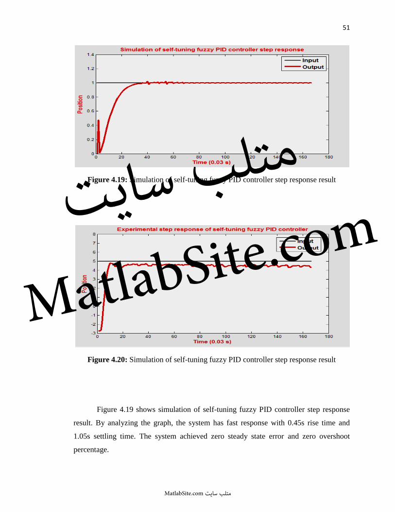
result. By analyzing the graph, the system has fast response with 0.45s rise time and

1.05s settling time. The system achieved zero steady state error and zero overshoot

percentage.

متلب سایت

MatlabSite.com


52

Figure 4.20 shows experimental step response result of self tuning fuzzy PID

controller. From the graph obtained, it’s clear that the system has fast response with 0.1s

rise time and 0.36s settling time. The system exhibits some steady state error of 6.25%

and it has a very small overshoot percentage of 2.22%.

Table 4.5: Simulation and experimental results of the controllers’ performance

specifications

Controller Rise

time Tr

Settling

time Ts

Overshoot

%OS

Steady

state

error %

Simulation PID 0.39s 1.29s 4.5% 0%

Fuzzy-PID 0.45s 1.05s 0% 0%

Experimental PID 0.12s 0.70s 27.27% 5%

Fuzzy-PID 0.10s 0.36s 2.22% 6.25%

From Table 4.4, it can be concluded that the system response of the pneumatic

system was improved significantly when applying conversional PID and self-tuning

Fuzzy-PID controllers. Self-tuning fuzzy-PID controller outperformed the conversional

PID controller with 2.22% overshoot only and faster response.

متلب سایت

MatlabSite.com


53

CHAPTER 5

CONCLUSION AND RECOMMENDATIONS

5.1 Conclusion

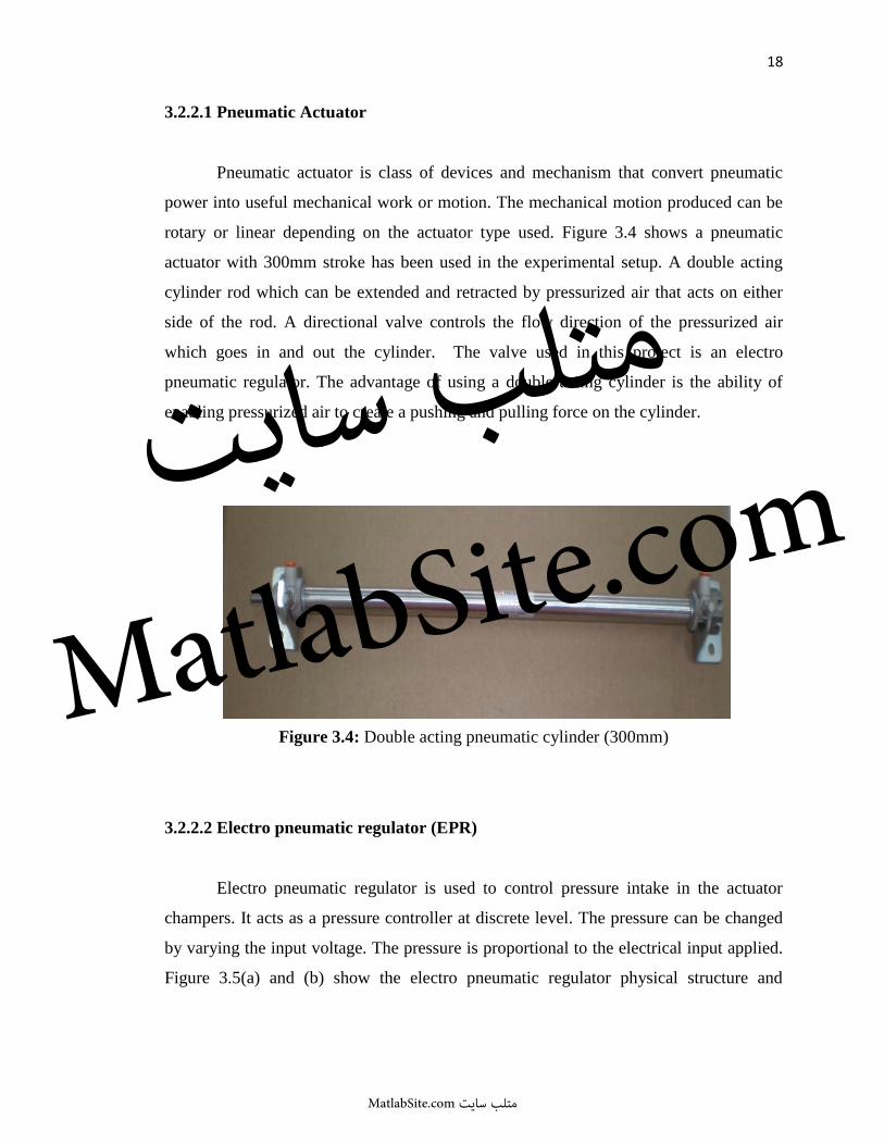
A pneumatic actuator is a mechanical device which converts the compressed air

energy into mechanical motion. The motion can be rotary or linear, depending on the

type of actuator. Many industries nowadays use pneumatic actuators in positioning,

clamping, gripping, drilling, and conveying operations in the process of manufacturing

and automation. This is due to the advantages pneumatic actuators offer over other types

of force actuators such as electromechanical and hydraulic actuators.

Although pneumatic actuators have many good attributes, achieving precise and

high-speed control of their systems is a challenge. This difficulty is due to the high-

order, time-variant actuator dynamics, and system nonlinearities like air compressibility,

static and coulomb friction, and pressure supply variations. This project presents the

process of modeling a pneumatic actuator system followed by designing controllers to

improve the system performance.

In this project, the pneumatic actuator system was modeled using system

identification toolbox. Input and output data were collected from the experimental

pneumatic actuator. The multi sine and single sine inputs where used with different

متلب سایت

MatlabSite.com


54

sampling times. Two model structures were selected which are Auto Regressive

Exogenous (ARX) and Auto Regressive Moving Average Exogenous (ARMAX). Model

estimation and validation were done by analyzing residual correlation and best fit

percentage.

From the analysis of the modeling results, multi sine models were unstable

because they have one of their poles outside the unit cycle. Besides, the percentage fit is

very low and not adequate for controller design purposes. For single sine models, very

good percentage fit was achieved when the sampling time is 0.01s; however, these

models fail to be adequate for controller design due to the very high gain in the

numerator of the transfer function. The models obtained when the sampling time was

0.03s are the best to be utilized in controller design because they have good percentage

fit and are stable too. Moreover, the numerator gain is acceptable.

To improve the system performance conventional PID and self tuning fuzzy-PID

controllers are designed. The coefficients of the PID controller are tuned using trial and

error method and Ziegler- Nichols method. Conventional PID controller achieved very

good performance in simulation, where the steady-state error is zero and the transient

response is fast with small overshoot percentage. When the conventional PID controller

was applied to the experimental set-up, a big overshoot percentage was observed. As a

result, the need to compensate for this error was important by using self tuning fuzzy

PID controller.

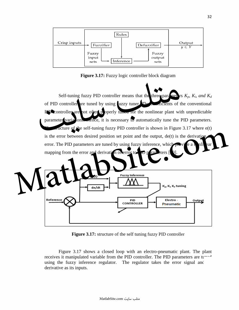
Self-tuning fuzzy PID controller means that the three parameters Kp, Ki and Kp of

PID controller are tuned by using fuzzy tuner. The controller used the error and the

derivative of the error as input to the fuzzy logic tuner. Both simulation and

experimental results of the self tuning fuzzy PID controller performed well in terms of

steady-state response and transient response.

متلب سایت

MatlabSite.com


55

The system response of the pneumatic system is improved significantly when

applying conversional PID and self-tuning Fuzzy-PID controllers. Self-tuning fuzzy-PID

controller outperformed the conversional PID controller with 2.22% overshoot only and

faster response.

5.2 Recommendations

Upon the completion of this project, there are some spaces for further

improvement. The effectiveness and accuracy of pneumatic actuator can be improved by

following the following suggestion are:

1. Optimize error of electro pneumatic regulator by controlling pressure of

the regulator valve.

2. Use neural network black box modeling.

3. Model the pneumatic actuator system with another model structure such

as Nonlinear Auto Regressive Exogenous (NLARX), Box- Jenkin, or

Output Error (OE).

4. Design a controller by using other controller such as LQR, neural

network controller or auto tuning PID controller.

متلب سایت

MatlabSite.com


56

CHAPTER 6

PROJECT MANAGEMENT

6.1 Introduction

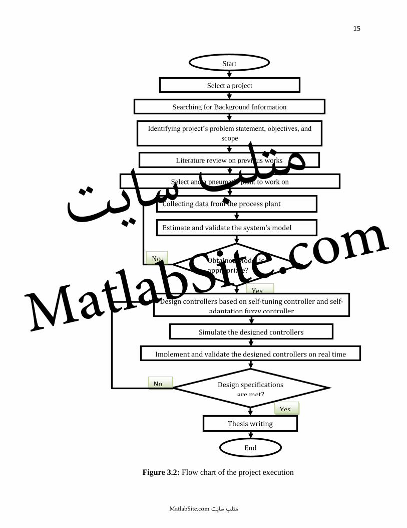
The objective of project management is to achieve all project goals with effective

project planning, organization and controlling resources within a specified time period.

The primary constrains in this project are the research scope, research time, research

budget and human resources to perform the required activity. Based on the stated

constrains, project schedule had been tabulated on a Gantt chart which gives a clear

guideline in time management of this project.

Next, cost estimation on the components is performed to insure minimal project

cost while keep working efficiently on the project to achieve the requirements. In this

process, market survey on different electronics suppliers is carried out; component

prices are then tabulated to compute the final cost.

6.2 Project Schedule

Table 6.1 shows the project Gantt chart for semester one. This table shows that

the FYP1 activity started from the very first week by choosing the project specialization

متلب سایت

MatlabSite.com


57

area. The following four weeks were utilized to produce the project proposal. Table 6.1

shows that the literature review activity occupies a period of five weeks. After that, the

experimental setup was connected and checked to ensure that all the hardware

components are working properly. In the last four weeks, the FYP1 presentation and

report documentation took place.

Table 6.1: Project Gantt chart (Semester 1)

N

o Activity

week

1 2 3 4 5 6 7 8 9 1

0

1

1

1

2

1

3

1

4

1

5

1 FYP area specialization

selection

2 FYP title discussion with

the supervisor

3 Project's objectives and

scope definitions

4 Literature review on

Pneumatic systems

5 Literature review

6 Connecting and checking

the pneumatic plant

7 Understanding all the plant

components

8 Methodology definition

9 Pneumatic plant data

acquisition and collection

10 Preparation of FYP1

presentation

11 FYP1 presentation

12 Documentation and report

writing

متلب سایت

MatlabSite.com


58

Table 6.2 shows the project Gantt chart for semester two. The table shows that

the FYP2 activity was started from the second week by doing the functionality testing of

the pneumatic actuator setup. In the following five weeks, the major activities were I/O

data collection and system modeling with some work on controller design.

Table 6.2 indicates clearly that controller design activity took the longest period

where it was performed starting from week five and ending in week eleven. After that,

experimental validation on the model and controller design was done to check if they

meet the design criteria. The Results were analyzed and discussed in the following three

week. Finally, the FYP2 seminar was held on the 13th

week and the thesis writing was

finished on the 18th

week.

Table 6.2: Project Gantt chart (Semester 2)

No. Activity

week

1 2 3 4 5 6 7 8 9 10 11 12 13 14 15-

18

1 Functionality test

2 Data Collection

3 Model estimation

4 Controller design

5

Experimental

Validation

6

Analysis and

discussion

7

Seminar

preparation

8 FYP seminar

9 Thesis writing

متلب سایت

MatlabSite.com


59

6.3 Cost Estimation

The pneumatic actuator system setup shown in Figure 3.3 is placed in process

control lab (P10) in faculty of electrical engineering. I did not design or fabricate the

experimental setup to do my project; however, it had already been in the lab and many

previous researchers used it in their projects. Table 6.3 shows the overall estimated cost

of the experimental setup.

Table 6.3: Main system components prices

Hardware component Cost per Piece (RM) Quantity Total (RM)

Electro-Pneumatic Regulator 909 2 1818

Communication Cable 135 3 405

LVDT (Position Sensor) 289 1 289

Pneumatic Actuator 98 1 98

Voltage Supply 12V 25 1 25

Test Table 100 1 100

Air Compressor 249 1 249

Air Tubing 50 1 50

Air Tubing 50 1 50

NI DAQ card (NI SCB-68) 350 1 350

(PCI) card (NI SCB-68) 500 1 500

Computer system 1000 1 1000

Shielded cables 300 2 600

Other Electronic Component 50

Total 5584

متلب سایت

MatlabSite.com


60

REFERENCES

1. Ali, Hazem I., Et Al. "A Review of Pneumatic Actuators (Modeling and

Control)."Australian Journal of Basic and Applied Sciences 3.2 (2009): 440-454.

2. Wang, J., J. Pu, Et Al. (1999). "A Practical Control Strategy for Servo-Pneumatic

Actuator Systems." Control Engineering Practice 7(12): 1483-1488.

3. Shih, M.-C. And S.-I. Tseng (1995). "Identification and Position Control of a Servo

Pneumatic Cylinder." Control Engineering Practice 3(9): 1285-1290.

4. Pandian, Shunmugham R., Et Al. "Pressure Observer-Controller Design for

Pneumatic Cylinder Actuators." Mechatronics, IEEE/ASME Transactions on 7.4

(2002): 490-499.

5. Zhihong, R. And G. M. Bone (2008). "Nonlinear Modeling and Control of Servo

Pneumatic Actuators." Control Systems Technology, IEEE Transactions on 16(3):

562-569.

6. Wang, J., J. D. Wang, Et Al. (2004). "Identification of Pneumatic Cylinder Friction

Parameters Using Genetic Algorithms." Mechatronics, Ieee/Asme Transactions on

9(1): 100-107.

7. Nguyen Thanh, T., T. Dinh Quang, Et Al. (2011). Identification of a Pneumatic

Actuator Using Non-Linear Black-Box Model. Control, Automation and Systems

(Iccas), 2011 11th International Conference.

8. Žilić, T., D. Pavković, Et Al. (2009). "Modeling And Control Of A Pneumatically

Actuated Inverted Pendulum." Isa Transactions 48(3): 327-335.

9. Bogdan, Codres, Et Al. "Identification of A Nonlinear Pneumatic Servo System

Using Modular Neural Networks."

10. Ning, Y., M. Betemps, Et Al. (1991). A Servocontrolled Pneumatic Actuator for

Small Movement-Application to an Adaptive Gripper. Advanced Robotics, 1991.

'Robots In Unstructured Environments', 91 Icar., Fifth International Conference.

11. Filipovic, V., N. Nedic, Et Al. (2011). "Robust Identification Of Pneumatic

ServoActuators In The Real Situations." Forschung Im Ingenieurwesen 75(4): 183-

196.

متلب سایت

MatlabSite.com


61

12. Chiang, Chiang-Cheng, and Mon-Han Chen. "Robust Adaptive Fuzzy Control of

Uncertain Nonlinear Time-Delay Systems with an Unknown Dead-Zone." Fuzzy

Systems, 2008. Fuzz-Ieee 2008. (IEEE World Congress on Computational

Intelligence). Ieee International Conference On. IEEE, 2008.

13. Chillari, S., S. Guccione, And G. Muscato. "An Experimental Comparison between

Several Pneumatic Position Control Methods." Decision and Control, 2001.

Proceedings of the 40th IEEE Conference On. Vol. 2. IEEE, 2001.

14. Yamazaki, M. And S. Yasunobu (2007). An Intelligent Control for State-Dependent

Nonlinear Actuator and Its Application to Pneumatic Servo System. Sice, 2007

Annual Conference.

15. Sunar, N. H., M. F. Rahmat, Et Al. (2013). Identification and Self-Tuning Control of

Electro-Pneumatic Actuator System with Control Valve. System Engineering and

Technology (ICSET), 2013 IEEE 3rd International Conference.

16. Malaysia, Melaka. "Non-Linear Modeling and Cascade Control of an Industrial

Pneumatic Actuator System." Australian Journal of Basic and Applied Sciences 5.8

(2011): 465-477.

17. Rahmat, M. F., Et Al. "Identification and Non-Linear Control Strategy for Industrial

Pneumatic Actuator." International Journal of Physical Sciences 7.17 (2012): 2565-

2579.

18. Lai, W. K., M. F. Rahmat, and N. Abdul Wahab. "Modeling and Controller Design

of Pneumatic Actuator System with Control Valve." International Journal on Smart

Sensing and Intelligent System 5.3 (2012): 624-644.

19. Sunar, N. H., M. F. Rahmat, Et Al. (2013). Application of Optimization Technique

for PID Controller Tuning In Position Tracking Of Pneumatic Actuator System.

Signal Processing and Its Applications (CSPA), 2013 IEEE 9th International

Colloquium.

20. Zulfatman and M.F. Rahmat, “Application of Self-tuning Fuzzy PID Controller on

Industrial Hydraulic Actuator Using System Identification Approach”, International

Journal on Smart Sensing and Intelligent System. Vol.2. No 2, 2009.

متلب سایت

MatlabSite.com


62

APPENDIX A

Electro-pneumatic Regulator

ITV1000/2000/3000

Standard Specifications

Straight type Right angle type

JIS Symbol Rated pressure

(MP

a)

Out

put p

ress

ure

This range is outside of the control (output).

0.005 MPa 0

0 100 Input signal (%F.S.)

Graph (1) Input/output characteristics chart

متلب سایت

MatlabSite.com


63

ITV101_ ITV103_ ITV105_

Model ITV201_ ITV203_ ITV205_

ITV301_ ITV303_ ITV305_

Minimum supply pressure Set pressure +0.1 MPa

Maximum supply pressure 0.2 MPa 1.0 MPa

Set pressure range Note 1) 0.005 to 0.1 MPa 0.005 to 0.5 MPa 0.005 to 0.9 MPa

Voltage 24 VDC 10%, 12 to 15 VDC

Power supply Current Power supply voltage 24 VDC type: 0.12 A or less

consumption Power supply voltage 12 to 15 VDC type: 0.18 A or less

Current type Note 2) 4 to 20 mA, 0 to 20 mA (Sink type)

Input signal Voltage type 0 to 5 VDC, 0 to 10 VDC

Preset input 4 points

Input Current type 250 Ω or less

Voltage type Approx. 6.5 kΩ

impedance

Preset input

Approx. 2.7 kΩ

Note 3) Analog output

1 to 5 VDC (Load impedance: 1 kΩ or more)

Output signal 4 to 20 mA (Sink type) (Load impedance: 250 Ω or less)

(monitor

NPN open collector output: Max. 30 V, 30 mA

output) Switch output

PNP open collector output: Max. 30 mA

Linearity Within 1% (full span)

Hysteresis Within 0.5% (full span)

Repeatability Within 0.5% (full span)

Sensitivity Within 0.2% (full span)

Temperature characteristics Within 0.12% (full span)/C

Output pressure Accuracy 3% (full span)

display Minimum unit MPa: 0.01, kgf/cm2: 0.01, bar: 0.01, PSI: 0.1 Note 4), kPa: 1

Ambient and fluid temperature 0 to 50C (with no condensation)

Enclosure IP65

ITV10__ Approx. 250 g (without options)

Weight ITV20__ Approx. 350 g (without options)

ITV30__ Approx. 645 g (without options)

Note 1) Please refer to “Graph (1)”, relation to the differences between the set pressure and input. Additionally, refer to page 14-8-29 for the set pressure range by units of standard measured pressure. Additionally, refer to page 14-8-29 as maximum set pressure differs on unit of standard measure.

Note 2) 2-wire type 4 to 20 mA is not available. Power supply voltage (24 VDC or 12 to 15 VDC) is required. Note 3) Select either analog output or switch output. Further, when switch output is selected, select either

NPN output or PNP output. Note 4) The minimum unit for ITV205_ is 1PSI. Note 5) The above characteristics are confined to the static state. When air is consumed on the output side, the pressure may fluctuate.

3 ∗ Switch output/PNP output T ∗ NPTF 2 1/4 (1000, 2000, 3000 type) B ∗ Flat bracket

4 ∗ Analog output 4 to 20 mA (Sink type) F ∗ G 3 3/8 (2000, 3000 type) C ∗ L-bracket

∗ Option ∗ Option 4 1/2 (3000 type) ∗ Option

14-8-14

متلب سایت

MatlabSite.com


64

Electro-pneumatic Regulator Series ITV1000/2000/3000

rSpacer SMC REGULATOR

ITV20__

ITV2000

App

rox.

189

Ap

prox

. 133

eL-bracket

178

qAF30 wAFM30

REGU LAT OR ITV30__

ITV3000

App

rox.

243

Appr

ox. 1

72

234

qAF40 wAFM40

Combinations Standard Combination Combination

specifications possible not possible

∗ ITV10__ models are not applicable.

Sym

bol Applicable model

Specifications ITV20__

ITV30__

Set pressure max. 0.1 MPa 1

Stan

dards

pecif

ica

tions



Connection Rc 1/4 02



Acces- Bracket B

sories Bracket C

Optio

nalsp

ecific

ation

s

Connection NPT1/4 N02



Connection G 1/4 F02



Modular Products and Accessory Combinations

∗ ITV10__ models are not applicable.

Applicable products and accessories Applicable model

ITV20__

ITV30__

q Air filter AF30 AF40

w Mist separator AFM30 AFM40

e L-bracket B310L B410L

r Spacer Y30 Y40

t Spacer with L-bracket (e + r) Y30L Y40L

F.R.L. AV AU AF AR IR VEX AMR ITV IC VBA VE_ VY1 G

Accessory (Option)/Part No.

Description Part no. Dimensions

ITV10__ ITV20__ ITV30__ Flat bracket

Flat bracket P3020114 100

(Mounting thread is not included.)

L-bracket INI-398-0-6

(Mounting thread is not included.)

5 2 4 0 2 2

Cable

conn

ector Straight TM-4DSX3HG4

type 3 m

PPA

AL

L-bracket

7

25

1 5 4

x

R

30 3 2.3

.

5

36

50

Right angle TM-4DLX3HG4 22

type 3 m

4 x ø7

_36

40

84

60

12

1.6

20

8 x ø4.5 50

4 x ø5.5

40

36

22

14

7 5

70

22

36

4 0

8 x ø4.5 4 x ø5.5

متلب سایت

MatlabSite.com


65

Series ITV1000/2000/3000

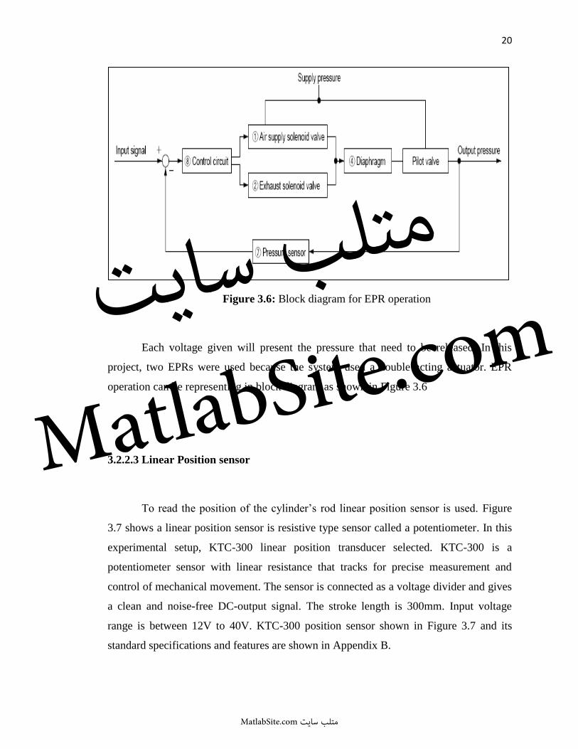
Working Principle When the input signal rises, the air supply solenoid valve q turns ON, and the exhaust solenoid valve w turns OFF. Therefore, supply pressure passes through the air supply solenoid valve q and is applied to the pilot chamber e. The pressure in the pilot chamber e increases and operates on the upper surface of the diaphragm r. As a result, the air supply valve t linked to the diaphragm r opens, and a portion of the supply pressure becomes output pressure. This output pressure feeds back to the control circuit i via the pressure sensor u. Here, a correct operation functions until the output pressure is proportional to the input signal, making it possible to always obtain output pressure proportional to the input signal.

Working Principle Diagram Pressure display

Power supply i Control Output signal

Input signal circuit

Pressure display

Power supply

q Air supply w Exhaust

i Control Output signal solenoid solenoid

Input signal circuit valve

valve

EXH

q Air supply w Exhaust

solenoid

solenoid u Pressure

valve

valve

r Diaphragm sensor

EXH e Pilot

y Exhaust chamber

valve

u Pressure sensor

r Diaphragm e Pilot chamber t Supply EXH

valve

t Supply valve

SUP OUT SUP OUT

EXH

ITV1000 ITV2000, 3000

Block diagram Input signal

i Control circuit

Supply pressure q Air supply solenoid valve

Output pressure r Diaphragm Pilot valve

w Exhaust solenoid valve u Pressure sensor

متلب سایت

MatlabSite.com


66

Electro-pneumatic Regulator Series ITV1000/2000/3000 Series ITV101_

Linearity Hysteresis Repeatability

1.0 1.0

0.10

Out

put d

evia

tion

fact

or

(%F.

S.)

Out

Out

put d

evia

tion

fact

or

(%F.

S.)

0.5 0.5

Set

pre

ssur

e (M

Pa)

0.08

0.06 0.0 Return

0.0

0.04

–0.5 –0.5

0.02

0.00 25 50 75 100

–1.0 25 50 75 100

–1.0 2 4 6 8 10

0 0 0

Input signal (%F.S.) Input signal (%F.S.) Repetition

Pressure Characteristics

Set pressure: Flow Characteristics

Supply pressure: Relief Flow Characteristics

Supply pressure:

0.05 MPa 0.2 MPa 0.2 MPa

Out

put d

evia

tion

fact

or (%

F.S

.)

1.0 0.15 0.25

0.5

Set

pre

ssur

e (M

Pa)

0.20

Set

pre

ssur

e (M

Pa)

Set point 0.10

0.15

0.0

0.05 0.10

–0.5 0.05

–1.0

0.3

0 20 40 60 80 100

0.000

0.0 0.1 0.2 20 40 60 80

Supply pressure (MPa) Flow rate ( /min (ANR)) Flow rate ( /min (ANR))

F.R.L. AV AU AF AR IR VEX AMR ITV IC

Series ITV201_

Linearity Hysteresis Repeatability

0.10 1.0 1.0

0.09

Out

put d

evia

tion

fact

or

(%F.

S.)

Out

put d

evia

tion

fact

or

(%F.

S.)

0.08 0.5 Out 0.5

Set

pre

ssur

e (M

Pa)

0.07

0.06 0.0

0.0

0.05

0.04 Return

0.03

–0.5 –0.5

0.02

0.01

0.00 25 50 75 100

–1.0 25 50 75 100

–1.0 2 4 6 8 10

0 0 0

Input signal (%F.S.) Input signal (%F.S.) Repetition

VBA VE_ VY1 G PPA AL

Pressure Characteristics

Set pressure:

0.05 MPa

(%F.

S.) 1.0

0.5

fact

or Set point

0.0

devi

atio

n

–0.5

Out

put

–1.0

0.0 0.1 0.2 0.3

Supply pressure (MPa)

Flow Characteristics Supply pressure:

0.2 MPa

0.15

(MPa

)

0.10

pres

sure

0.05

Set

0 200 400 600

Flow rate ( /min (ANR))

Relief Flow Characteristics Supply pressure:

0.2 MPa

0.25

(MP

a) 0.20

0.15

Set p

ress

ure

0.10

0.05

0.000 200 400 600 800

Flow rate ( /min (ANR))

متلب سایت

MatlabSite.com


67

Electro-pneumatic Regulator Series ITV1000/2000/3000

Dimensions ITV10__ Flat bracket Note) Do not attempt to rotate, as the cable connector does not turn.

Cable connector (4-wire) Cable connector (4-wire)

Right angle type Straight type

_50 4 x ø7

Mounting hole ( 3 1 )

SMCE

P REGULATOR SMC E

P RE GULAT OR

RESET

52

SET

UNLOCK LOCK ITV1000 ITV1000

Setting part

84

100

12.5 M12 x 1

Cable connection threads

( 1 1 )

SMCE

P REGULATOR

MPa

ITV10

INPUT 0~10VDC

Rc1/8

OUTPUT 0.005~0.5MPa

M3 x 0.5 MADE IN JAPAN GY

7 1

Exhaust port

Solenoid valve

EXH Solenoid valve EXH

G 2 OUT

SUP (1) OUT (2)

19.5 EXH (3)

1 1

1 2

40 Flat bracket 2 x Rc1/8, 1/4

P3020114

Port size

(Optional)

4 x M4 x 0.7 thread depth 6 mm through Mounting hole

L-bracket

F.R.L. AV AU AF AR IR VEX AMR ITV IC VBA VE_ VY1 G PPA AL

G

15 .5

R3

2 5 7

(10) 30

(7) 36 L-bracket

INI-398-0-6

(Optional)

2 OUT

22 2.3

45 2 x Rc1/8, 1/4 SUP port, OUT port

متلب سایت

MatlabSite.com


68

APPENDIX B

KTC / KTF Linear sensor 75-1000 mm Potentiometric transducer with conductive track suitable for measurment, monitoring and control of mechanical strokes. Critical in providing a smooth output, mechanically dependent on the stable glide of the shaft and wiper on the element’s surface. Applications such as industrial controls, robotics, process systems or replacement of a linear voltage differential transformer (LVDT) are ideal uses for this versatile, reliable model.

Features:

Case ... Brushes ... Resistance track ... Control rod ... Resolution ... Repeatability ... Life time ...

Electrical connections ...

Temperature range ...

.Anodised aluminium ..Noble metal

.. Conductive plastic on polymer base ..Stainless steel

.. Infinitie .within 0,013 mm

..>25x106 meters or >100x106 cycles ...4-pole connector to DIN

..43650 ISO 4400 . -55ºC- +125ºC

Output options

Contact Standard 4-20 mA 1 - supply - supply 2 Signal 0-V+- 4-20 mA 3 + supply + 15-35 V

Mechanical dimensions KTC

Max supply voltage at 70°C .................................................... .40 VDC Recommended cursor current ... .......................................... .. <1mMechanical dimensions KTF Rod end bearing (KTC-01)

Coupling join

KTC KTC7 100 150 225 300 375 450 525 600 750 900 KTF100

Total el. travel (T.E) mm 76 102 150 229 305 381 457 533 610 762 914 1016 -

Active el. travel (A.E) mm 75 100 150 226 302 378 455 531 607 759 912 1013

Resistance (±20%) k 2,5 3,4 5,0 2,4 3,2 4,0 4,8 5,6 6,4 8,0 9,6 10,7

Independent linearity ±% 0,07 0,07 0,07 0,07 0,07 0,07 0,05 0,05 0,05 0,05 0,05 0,05

Mechanical travel (M.T) mm Dimensions KTC (A) mm

79 104 155 231 307 384 139 164 215 291 367 444

460 536 612 765 917 1019 520 596 672 825 977

متلب سایت

MatlabSite.com


Date post:	02-May-2018
Category:	Documents
Upload:	lamnhu
View:	218 times
Download:	2 times

DECLARATION OF THESIS ... -...

Documents