HAL Id: tel-01056746 https://tel.archives-ouvertes.fr/tel-01056746 Submitted on 20 Aug 2014 HAL is a multi-disciplinary open access archive for the deposit and dissemination of sci- entific research documents, whether they are pub- lished or not. The documents may come from teaching and research institutions in France or abroad, or from public or private research centers. L’archive ouverte pluridisciplinaire HAL, est destinée au dépôt et à la diffusion de documents scientifiques de niveau recherche, publiés ou non, émanant des établissements d’enseignement et de recherche français ou étrangers, des laboratoires publics ou privés. Decoding of block and convolutional codes in rank metric Antonia Wachter-Zeh To cite this version: Antonia Wachter-Zeh. Decoding of block and convolutional codes in rank metric. General Mathemat- ics [math.GM]. Université Rennes 1, 2013. English. NNT : 2013REN1S126. tel-01056746
Transcript
HAL Id: tel-01056746https://tel.archives-ouvertes.fr/tel-01056746
Submitted on 20 Aug 2014
HAL is a multi-disciplinary open accessarchive for the deposit and dissemination of sci-entific research documents, whether they are pub-lished or not. The documents may come fromteaching and research institutions in France orabroad, or from public or private research centers.
L’archive ouverte pluridisciplinaire HAL, estdestinée au dépôt et à la diffusion de documentsscientifiques de niveau recherche, publiés ou non,émanant des établissements d’enseignement et derecherche français ou étrangers, des laboratoirespublics ou privés.
Decoding of block and convolutional codes in rankmetric
Antonia Wachter-Zeh
To cite this version:Antonia Wachter-Zeh. Decoding of block and convolutional codes in rank metric. General Mathemat-ics [math.GM]. Université Rennes 1, 2013. English. NNT : 2013REN1S126. tel-01056746
Silva, Kschischang et Kötter [SKK08] ont montré que les codes de Gabidulin relevés (lifted) résultaienten des codes de sous-espaces presque optimaux pour le codage réseau linéaire aléatoire. Les codes deGabidulin sont les analogues en métrique rang des codes de Reed–Solomon et ils ont été introduits parDelsarte, Gabidulin et Roth [Del78, Gab85, Rot91]. Un code en métrique rang de longueur n ≤ m peutêtre considéré comme un ensemble de matricesm×n dans un corps Vni Fq ou, de manière équivalente,comme un ensemble de vecteurs de longueur n dans l’extension de corps Fqm . Le poids rang d’un tel«mot» est simplement le rang de sa représentation matricielle et la distance rang entre deux mots estle rang de leur diUérence. Ces déVnitions s’appuient sur le fait que la distance rang est une métrique.
v
Plusieurs constructions de codes et des propriétés de base de la métrique rang possèdent de fortes
similarités avec les codes en métrique de Hamming.
SuperVciellement, un code de Gabidulin relevé est un code de sous-espaces spécial où chaque mot de
code est l’espace des lignes d’une matrice[I CT
], où I désigne la matrice identité et C est un mot de
code (en représentation matricielle) d’un code de Gabidulin Vxé.
Cette thèse traite des codes en bloc et des codes convolutifs en métrique rang avec l’objectif de
développer et d’étudier des algorithmes de décodage eXcaces pour ces deux classes de codes. Cette
thèse est structurée comme suit.
Le chapitre 1 donne une brève motivation pour l’utilisation des codes en métriques rang dans le
cadre de l’application au codage réseau linéaire aléatoire et présente un aperçu de cette thèse.
Le chapitre 2 fournit une introduction rapide aux codes en métrique rang et leurs propriétés. Après
avoir introduit des notations pour les corps Vnis et les bases normales, nous indiquons les déVnitions
des codes en bloc et codes convolutifs en général. On donne quelques propriétés élémentaires et le
principe de base du décodage des codes en bloc. Les codes de Gabidulin peuvent être déVnis comme
des codes d’évaluation de polynômes linéarisés, pour cette raison, nous déVnissons cette classe des
polynômes et montrons comment on peut eUectuer les opérations mathématiques de base sur ces
polynômes.
La dernière section du chapitre 2 couvre les codes en métriques rang. On déVnit d’abord la métrique
rang et on donne des propriétés de base pour les codes en métrique rang (par exemple, les équivalents
des bornes de Singleton et de Gilbert–Varshamov). Ensuite, on déVnit les codes de Gabidulin, on montre
qu’ils atteignent la borne supérieure de Singleton pour la cardinalité et on donne leur matrices généra-
trice et de contrôle. Nous généralisons par la suite leur déVnition aux codes de Gabidulin entrelacés
et on montre explicitement comment les codes de Gabidulin relevés constituent un code de sous-espaces.
Dans le chapitre 3, on considère des approches eXcaces pour décoder les codes de Gabidulin. La
première partie de ce chapitre traite des algorithmes rapides pour les opérations sur les polynômes
linéarisés. Dans ce contexte, on analyse la complexité des approches connues pour les opérations
dans un corps Vnis avec des bases normales ainsi que pour les opérations mathématiques avec des
polynômes linéarisés. Ensuite, nous présentons de nouveaux algorithmes en temps sous-quadratique
pour accomplir eXcacement la composition linéarisé et l’algorithme d’Euclide linéarisé.
La deuxième partie de ce chapitre résume tout d’abord les techniques connues pour le décodage
jusqu’à la moitié de la distance rang minimale (bounded minimum distance decoding) des codes de
Gabidulin, qui sont basées sur les syndromes et sur la résolution d’une équation clé. Ensuite, nous
présentons et nous prouvons un nouvel algorithme eXcace pour le décodage jusqu’à la moitié de la
distance minimale des codes de Gabidulin. Cet algorithme peut être considéré comme un équivalent
de l’algorithme de Gao pour le décodage des codes de Reed–Solomon. Nous montrons comment
l’algorithme d’Euclide linéarisé peut être utilisé dans ce contexte pour obtenir directement le polynôme
de degré restreint d’évaluation du mot de code estimé. De plus, nous étendons cet algorithme de
décodage aVn de corriger non seulement des erreurs, mais aussi deux types d’eUacements en métrique
rang: eUacements de lignes et de colonnes.
vi
Le codage réseau linéaire aléatoire peut directement proVter d’un tel algorithme de décodage eXcace
pour les codes Gabidulin, car il accélère immédiatement la reconstruction des paquets transmis et donc
il réduit le délai nécessaire. L’extension de notre algorithme de décodage aux combinaisons d’erreurs et
d’eUacements est cruciale pour gérer les pertes de paquets dans le codage réseau linéaire aléatoire.
Le chapitre 4 est consacré aux codes de Gabidulin entrelacés et à leur décodage au-delà de la moitié
de la distance rang minimale. Un mot de code d’un code de Gabidulin entrelacé peut être considérécomme s mots de code parallèles de s codes de Gabidulin normaux (pas nécessairement diUérents). Cessmots de code sont corrompus par smatrices d’erreur. Lorsque ces smatrices d’erreur additives ont unespace de lignes ou de colonnes en commun, il est possible de décoder les codes de Gabidulin entrelacésau-delà de la moitié de la distance rang minimale avec une grande probabilité. Jusqu’à présent, deuxapproches probabilistes pour le décodage unique sont connues pour ces codes.
Dans ce chapitre, nous décrivons d’abord les deux approches connues pour le décodage uniqueet nous tirons une relation entre eux et leurs probabilités de défaillance. Ensuite, nous présentonsun nouvel algorithme de décodage des codes de Gabidulin entrelacés basé sur l’interpolation despolynômes linéarisés. Nous prouvons la justesse de ses deux étapes principales — l’interpolation et larecherche des racines — et montrons que chacune d’elles peut être eUectuée en résolvant un systèmed’équations linéaires.
On peut utiliser l’algorithme comme algorithme de décodage en liste des codes de Gabidulin en-trelacés, qui garantit de trouver tous les mots de code dans un certain rayon. Cependant, la taille de laliste, et donc aussi au pire la complexité d’algorithme du décodage en liste, peut devenir exponentielleen la longueur du code. On peut également utiliser notre décodeur comme un décodeur probabilisteunique, en temps quadratique, avec le même rayon de décodage et la même borne supérieure de laprobabilité de défaillance que les décodeurs connus. En clair, pour n’importe quel décodeur unique,au-delà de la moitié de la distance rang minimale il y aura toujours une probabilité de défaillance car iln’existe pas toujours une solution unique. Nous généralisons notre décodeur pour décoder en mêmetemps des erreurs et des eUacements de lignes et de colonnes.
Dans le codage réseau linéaire aléatoire, un code de Gabidulin relevé entrelacé contient les espacesdes lignes de
[I C(0)T C(1)T . . . C(s)T
], où les C(i), pour tout i ∈ [1, s], sont des mots de code des
codes de Gabidulin sous-jacents. Ainsi, par rapport aux codes de Gabidulin relevés, le relèvement(lifting) des codes entrelacés de Gabidulin réduit relativement les frais généraux, qui sont causés par lamatrice d’identité jointe.
Jusqu’à présent, aucun algorithme de décodage en liste en temps polynomial pour les codes deGabidulin n’est connu et en fait il n’est même pas clair que cela soit possible. Cela nous a motivé àétudier, dans le chapitre 5, les possibilités du décodage en liste en temps polynomial des codes enmétrique rang. Cette analyse est eUectuée par le calcul de bornes sur la taille de la liste des codes enmétriques rang en général et des codes de Gabidulin en particulier.
On rappelle d’abord les bornes connues sur le décodage en liste des codes en métrique de Hamming,puis on déduit des bornes sur la taille de la liste des codes en métrique rang. Nous considérons en fait lenombre maximal de mots de code dans une boule en métrique rang de rayon τ , qui est appelé la taille(maximale) de la liste. Étonnamment, ces trois nouvelles bornes révèlent toutes un comportement descodes en métrique rang qui est complètement diUérent de celui des codes en métrique de Hamming.
vii
La première borne montre que la taille de la liste pour un code de Gabidulin de longueur n et
de distance rang minimale d peut devenir exponentielle quand τ est au moins le rayon de Johnson
n−√
n(n− d). Cela implique qu’il ne peut pas exister un algorithme de décodage en liste en temps
polynomial pour les codes de Gabidulin au-delà du rayon de Johnson. Il est intéressant de noter qu’on
ne sait pas ce qui se passe pour les codes de Reed–Solomon si τ est légèrement supérieur au rayon de
Johnson.
Notre deuxième borne est une borne supérieure sur la taille de la liste de tous les code en métrique
rang, qui est prouvé par des liens entre les codes de rang constant (constant-rank codes) et les codes de
dimension constante (constant-dimension codes).
Ce sont précisément ces liens qui nous permettent de dériver la troisième borne. Avec cette borne,
nous pouvons prouver qu’il existe un code en métrique rang dans Fqm de longueur n ≤ m tel que
la taille de la liste peut devenir exponentielle pour tout τ supérieur à la moitié de la distance rang
minimale. Cela implique d’une part qu’il n’y a pas de borne supérieure polynômiale, semblable à la
borne de Johnson en métrique de Hamming, et d’autre part que notre borne supérieure est presque
optimale.
La pertinence d’une algorithme de décodage en liste pour le codage réseau linéaire aléatoire est
évidente, car un tel décodeur pourrait tolérer plus de paquets erronés qu’un décodeur de distance
minimale bornée pour les codes de Gabidulin relevés.
EnVn, dans le chapitre 6, on introduit des codes convolutifs en métrique rang. Ce qui nous motive à
considérer ces codes est le codage réseau linéaire aléatoire multi-shot, où le réseau inconnu varie avec
le temps et est utilisé plusieurs fois. Les codes convolutifs créent des dépendances entre les utilisations
diUérentes du réseau aVn de se adapter aux canaux diXciles.
Nous proposons des mesures de la distance pour les codes convolutifs en métrique rang par analogie
avec la métrique de Hamming, à savoir la distance rang libre (free rank distance), la distance rang active
des lignes (active row rank distance) et la pente (slope) de la distance rang active des lignes, et on prouve
des bornes supérieures pour ces mesures. Basé sur des codes en bloc en métrique rang (en particulier
les codes de Gabidulin), nous donnons deux constructions explicites des codes convolutifs en métrique
rang : une construction à haut taux basée sur la matrice de contrôle et une construction à faible taux
basée sur la matrice génératrice. Les deux déVnissent des codes (partial) unit memory et atteignent la
borne supérieure de la distance rang libre.
Les codes en bloc sous-jacents nous permettent de développer un algorithme de décodage des erreurs
et des eUacements eXcace pour la deuxième construction, qui garantit de corriger toutes les séquences
d’erreurs de poids rang jusqu’à la moitié de la distance rang active des lignes. La complexité de
l’algorithme de décodage est cubique en la longueur de la séquence transmise. Nous prouvons sa
justesse et décrivons explicitement comment nos codes convolutifs en métrique rang peuvent être
appliqués au codage réseau linéaire aléatoire multi-shot.
Un résumé et un aperçu des problèmes futurs de recherche sont donnés à la Vn de chaque chapitre.Finalement, le chapitre 7 conclut cette thèse.
Fq Finite Veld of order qFqm Extension Veld of Fq of degree mFs×nq Set of all s× n matrices over Fq
Fnqm = F1×n
qm Set of all row vectors of length n over Fqm
B = β0, β1, . . . , βm−1 Basis of Fqm over Fq
B⊥ = β⊥0 , β
⊥1 , . . . , β
⊥m−1 Dual basis (to B) of Fqm over Fq
BN = β[0], β[1], . . . , β[m−1] Normal basis of Fqm over Fq with normal element β
B⊥N = β⊥[0], β⊥[1], . . . , β⊥[m−1] Dual normal basis (to BN ) with dual normal element β⊥
β = (β0 β1 . . . βm−1) Ordered basis of Fqm over Fq
Tr(a) =∑m−1
i=0 a[i] Trace function of a ∈ Fqm
Tm ∈ Fm×mq Multiplication table for a given normal basis
comp(Tm) Number of non-zero elements of Tm
Sets and Vector Spaces
[i, j] Short form for i, i+ 1, . . . , jdim(V) Dimension of a vector space VPq(n) Projective space = set of all subspaces of Fn
q
Gq(n, r) Grassmannian = set of all subspaces of Fnq of dimension r[
nr
]q-binomial = cardinality of Gq(n, r)
Matrices
A =(Ai,j
)i∈[0,m−1]
j∈[0,n−1]m× n matrix
a = (a0 a1 . . . an−1) (Row) vector of length n(aT )↑i, (aT )↓i Cyclic up/down shift of a column vector aT
rk(A) Rank of matrix Aker(A) Right kernel (= nullspace) of matrix Aim(A) = Cq (A) Image ofA = column space of A (over Fq)
Rq (A) Row space of A (over Fq)
B(e)R (a) = B(e)R (A) Ball of radius e in rank metric around a ∈ Fnqm
S(e)R (a) = S(e)R (A) Sphere of radius e in rank metric around a ∈ Fnqm
Is s× s identity matrix
qvans((a0 a1 . . . an−1)) s× n q-Vandermonde matrix for vector (a0 a1 . . . an−1)
xi
Contents
Linearized Polynomials
Lqm [x] Linearized polynomial ring in Fqm with indeterminate xLqm [x, y1, . . . , ys] Multivariate linearized polynomial ring in Fqm with indeter-
minates x, y1, . . . , ys
degq a(x) q-degree of linearized polynomial a(x)
a(x) Full q-reciprocal of a(x), deVned by ai = a[i]−i = a
[i]m−i
a(x) q-transform of a(x)a(b) = (a(b0) a(b1) . . . a(bn−1)) Evaluation of linearized polynomial a(x) at a vector b
Mu0,u1,...,udim(U)−1(x) Minimal subspace polynomial of a subspace U , where
u0, u1, . . . , udim(U)−1 is a basis of U
Block Codes
(n,M, d) Code (not necessarily linear) of length n, cardinality M and
minimum distance d (in some given metric)
[n, k, d] Linear code of length n, dimension k and minimum distance
d (in some given metric)
(n,M, d)R Code in rank metric (not necessarily linear) of length n,cardinality M and minimum rank distance d
[n, k, d]R Linear code in rank metric of length n, dimension k and
minimum rank distance d
MRD(n,M) Maximum rank distance code (not necessarily linear) of
length n and cardinality M
MRD[n, k] Linear maximum rank distance code of length n and dimen-
sion k
Gab[n, k] Gabidulin code of length n and dimension k
IGab[s;n, k(1), . . . , k(s)] Interleaved Gabidulin code of length n, elementary dimen-
sions k(i) and interleaving order s
CRqm(n,M, d, r) Constant-rank code (not necessarily linear) of length n, car-dinalityM , minimum rank distance d and rank r over Fqm
CDq(n,M, ds, r) Constant-dimension code of cardinality M , minimum sub-
space distance ds and dimension r (= subset of Gq(n, r))ARqm (n, d) Maximum cardinality of a code over Fqm of length n and
minimum rank distance d
ARqm (n, d, r) Maximum cardinality of a constant-rank code of length n,
minimum rank distance d and rank r over Fqm
ASq (n, ds, r) Maximum cardinality of a constant-dimension code in
Gq(n, r) with minimum subspace distance ds
xii
Contents
Convolutional Codes
Fq[D] Polynomial ring in Fq with indeterminate D
µ Memory of a convolutional generator matrix
νi, ν i-th and overall constraint length of a convolutional genera-
tor matrix
UM(n, k) Unit memory code of code rate R = k/n and ν = k
PUM(n, k|k(1)) Partial unit memory of code rate R = k/n and ν = k(1)
Acronyms
BMD bounded minimum distanceBRD bounded row distanceLEEA linearized extended Euclidean algorithmML maximum likelihoodMRD maximum rank distancePUM (partial) unit memoryRLNC random linear network coding
xiii
xiv
CHAPTER1Motivation and Overview
Error-correcting codes have their origin in Shannon’s seminal publication from 1948 [Sha48],
where he proved that nearly error-free discrete data transmission is possible over any noisy
channel when the code rate is less than the channel capacity. This statement is nowadays
called the (noisy) channel coding theorem. The channel capacity depends on the physical properties of
the channel and it is an active research area to determine the capacity of non-trivial communication
channels. However, the proof of the channel coding theorem is non-constructive and therefore it is
not clear how to construct error-correcting codes which actually achieve the Shannon limit. A steady
stream of publications and textbooks about code constructions, their properties and decoding methods
has emerged with Hamming’s class of codes [Ham50] and has not yet come to an end. For most data
transmission and data storage systems, the Hamming metric is the “proper” metric and codes deVned in
this metric practically perform quite well.
Quite recently, random linear network coding (RLNC) attracts a lot of attention. It is a powerful means
for spreading information in networks from sources to sinks (see e.g., [ACLY00, HKM+03, HMK+06]).
The operator channel was introduced by Kötter and Kschischang [KK08] as an abstraction of non-
coherent RLNC. In this model, the packets are assumed to be vectors over a Vnite Veld while the
internal structure of the network is unknown. Each node of the network forwards random linear
combinations of all packets received so far. Due to these linear combinations, one single erroneous
packet can propagate widely throughout the whole network and can render the whole transmission
useless. This strong error propagation makes error-correcting codes in RLNC essential in order to
reconstruct transmitted packets.
When the transmitted packets are considered as rows of a matrix, then the linear combinations of
the nodes are nothing but elementary row operations on this matrix. During an error- and erasure-free
transmission over the operator channel, the row space of the transmitted matrix is therefore preserved.
Based on this observation, Kötter and Kschischang [KK08] used subspace codes for error control in
RLNC. A subspace code is a non-empty set of subspaces of the vector space of dimension n over a
Vnite Veld and each codeword is a subspace itself. The so-called subspace distance is used as a distance
Silva, Kschischang and Kötter [SKK08] showed that lifted Gabidulin codes result in almost optimalsubspace codes for RLNC. Gabidulin codes are the rank-metric analogs of Reed–Solomon codes andwere introduced by Delsarte, Gabidulin and Roth [Del78, Gab85, Rot91]. Codes in rank metric, inparticular Gabidulin codes, can be seen as a set of matrices over a Vnite Veld. The rank of the diUerenceof two matrices is called their rank distance, which is induces a metric for matrix codes, the rank metric.
Informally speaken, a lifted Gabidulin code is a special subspace code, where each codeword isthe row space of a matrix
[I CT
], I denotes the identity matrix and C is a codeword (in matrix
representation) of a Vxed Gabidulin code.
1
1 Motivation and Overview
For this reason, codes in rank metric are an active research area in the context of RLNC. Apart
from RLNC [SKK08, Sil09, Gad09], the application of codes in rank metric ranges from cryptogra-
LK04, ALR13] and distributed storage systems [SRV12, RSKV13, SRKV13].
This dissertation deals with decoding approaches for block and convolutional codes in rank
metric. In the following overview of the thesis, we motivate our results with their application to
RLNC, but all of them are independently valid in a wider context of coding theory. Hence, we do
not explicitly explain the application of our results to RLNC or other possible applications within the
chapters (except for Chapter 6). This dissertation is structured as follows.
Chapter 2 provides a brief introduction to codes in rank metric and their properties. After giving
basic notations for Vnite Velds and normal bases, we state the deVnitions of block and convolutional
codes in general. We give some elementary properties and basic decoding principles for block codes.
Since Gabidulin codes can be deVned by evaluating linearized polynomials, we deVne this class of
polynomials and show how basic mathematical operations are performed on them. Finally, the last
section of Chapter 2 covers codes in rank metric. We Vrst deVne the rank metric and give basic
properties and bounds on the cardinality of codes in rank metric (namely, equivalents of the Singleton
and the Gilbert–Varshamov bound). Then, we deVne Gabidulin codes, show that they attain the
Singleton-like upper bound on the cardinality and give their generator and parity-check matrices. We
generalize this deVnition to interleaved Gabidulin codes and describe explicitly how lifted Gabidulin
codes constitute a class of subspace codes.
Within Chapter 3, eXcient approaches for decoding Gabidulin codes are considered. The Vrst part
of this chapter deals with fast algorithms for operations with linearized polynomials. In this context, we
analyze the complexity of known approaches and present new algorithms to accomplish the linearized
composition and the linearized extended Euclidean algorithm (LEEA) eXciently. The second part of this
chapter describes known syndrome-based decoding techniques and presents a new eXcient bounded
minimum distance (BMD) decoding algorithm for Gabidulin codes. Our algorithm uses the (fast) LEEA
in order to output directly the linearized evaluation polynomial of the estimated codeword. Further,
we show how our algorithm can be used for error-erasure decoding of Gabidulin codes. RLNC can
directly take advantage of such an eXcient decoding algorithm for Gabidulin codes, since it accelerates
immediately the reconstruction of the transmitted packets and reduces therefore the involved delay.
Chapter 4 is devoted to approaches for decoding interleaved Gabidulin codes. A codeword of an
interleaved Gabidulin code can be considered as s parallel codewords of usual Gabidulin codes. When
the s additive error matrices have one common row or column space, we can decode beyond half the
minimum rank distance with high probability. We Vrst describe two known approaches for unique
decoding of interleaved Gabidulin codes and derive a relation between them. Then, we present a new
interpolation-based decoding algorithm for interleaved Gabidulin codes. We prove the correctness
of its two main steps—interpolation and root-Vnding—and show that both can be carried out by
solving a linear system of equations. We outline how our decoder can be used as a (not necessarily
polynomial-time) list decoder as well as a quadratic-time probabilistic unique decoder. In this context,
we upper bound the failure probability of the unique decoder. In RLNC, a lifted interleaved Gabidulin
code consists of the row spaces of[I C(0)T C(1)T . . . C(s)T
], where the C(i), for all i ∈ [1, s], are
codewords of the underlying Gabidulin codes. Hence, compared to lifted Gabidulin codes, the lifting of
interleaved Gabidulin codes relatively reduces the overhead, which is caused by the appended identity
matrix.
2
So far, no polynomial-time list decoding algorithm for Gabidulin codes is known and it is not even
clear if it is possible at all. Therefore, Chapter 5 deals with bounds on list decoding block codes in
rank metric in general and Gabidulin codes in particular. We Vrst recall known bounds on list decoding
of codes in Hamming metric and then derive three bounds on list decoding codes in rank metric.
Surprisingly, the rank-metric bounds are all signiVcantly diUerent from the known bounds in Hamming
metric. In particular, we prove that in rank metric there exists no polynomial upper bound on the
list size similar to the Johnson bound in Hamming metric. Further, one of our bounds shows that the
list size can become exponential directly beyond the Johnson radius when decoding Gabidulin codes.
Remarkably, it is not known if this property holds for Reed–Solomon codes. The relevance of a list
decoding algorithm for RLNC is obvious, since such a decoder could tolerate more erroneous packets
than a BMD decoder for the (lifted) Gabidulin code.
Finally, Chapter 6 introduces convolutional codes in rank metric. The motivation of considering
such codes lies in multi-shot RLNC, where the unknown and time variant network is used several
times. Convolutional network codes create dependencies between the diUerent shots in order to cope
with diXcult channels. First, we deVne distance measures for convolutional codes in rank metric
and prove upper bounds on them. Then, we construct a special class of convolutional codes—partial
unit memory (PUM) codes—based on rank metric block codes in two diUerent ways. We presentan algorithm which eXciently decodes these PUM codes when both, errors and erasures occur andprove its correctness. The decoding complexity of this decoding algorithm is cubic in the length of atransmitted block. Further, it is explicitly described how lifting of these codes can be applied for errorcorrection in multi-shot RLNC.
Chapter 7 concludes this dissertation.
3
1 Motivation and Overview
4
CHAPTER2Introduction to Codes in Rank Metric
Codes in rank metric of length n ≤ m can be considered as a set ofm×nmatrices over a Vnite
Veld Fq or equivalently as a set of vectors of length n over the extension Veld Fqm . The rank
weight of such a “word” is simply the rank of its matrix representation and the rank distance
between two words is the rank of their diUerence. These deVnitions rely on the fact that the rank
metric is indeed a metric. Several code constructions and basic properties of the rank metric show
strong similarities to codes in Hamming metric.
Error-correcting codes in rank metric were Vrst considered by Delsarte in 1978 [Del78], who proved
a Singleton-like upper bound on the cardinality and constructed a class of codes achieving this bound.
This class of codes was reintroduced in 1985 by Gabidulin in his fundamental paper [Gab85], where in
addition several properties of codes in rank metric and an eXcient decoding algorithm were shown.
Since Gabidulin’s publication contributed signiVcantly to the development of error-correcting codes in
rank metric, the most famous class of codes in rank metric—the equivalents of Reed–Solomon codes—are
nowadays called Gabidulin codes. These codes can be deVned by evaluating non-commutative linearized
polynomials, proposed by Ore [Ore33a, Ore33b]. Independently of the previous work, Roth discovered
in 1991 codes in rank metric in order to apply them for correcting crisscross error patterns [Rot91].
This chapter gives a brief introduction to the theory of error-correcting codes in rank metric.
Section 2.1 provides deVnitions and notations used in this thesis for codes in Vnite Velds. Section 2.2
introduces linearized polynomials and their main properties. Finally, Section 2.3 deals with general
properties and explicit constructions of codes in the rank metric.
2.1 Codes over Finite Fields
Throughout this thesis, we consider algebraic codes over Vnite Velds and hence, this section introduces
notations and basic properties of Vnite Velds (Subsection 2.1.1) and codes over them. In Subsection 2.1.2,
we show properties of normal bases since they enable us to accomplish calculations in Vnite Velds
quite eXciently. We clarify our notations for block codes and explain well-known decoding principles
for block codes in Subsection 2.1.3: bounded minimum distance decoding, nearest codeword decoding
and list decoding. Further, we introduce notations and basic properties of convolutional codes in
Subsection 2.1.4.
2.1.1 Notations for Finite Fields
This subsection provides notations concerning Vnite Velds, without going into detail about their
theory. An extensive study of Vnite Velds, their properties and applications can be found in standard
literature about Vnite Velds, e.g., [LN96, MBG+93], and also in books about coding theory, e.g.,
[Ber84, Bla03, Rot06, HP10].
Let p be a prime, then Fp = 0, 1, . . . , p− 1 denotes the prime Veld of order p. Let q be a power of
5
2 Introduction to Codes in Rank Metric
the prime p, then we denote by Fq the Vnite Veld of order q. This Vnite Veld Fq contains q elements and
p is called its characteristic. An extension Veld (of extension degreem) of Fq is denoted by Fqm . This
extension Veld Fqm can be constructed from Fq and a polynomial p(x) of degreem, which is irreducible
in Fq and whose coeXcients are in Fq . For anym there is at least one such irreducible polynomial of
degree m [LN96, Corollary 2.11]. Since all Velds of the same size are isomorphic [LN96, Theorem 1.78],
the Veld Fqm does not depend on the explicit choice of p(x) and is isomorphic to the polynomial ring
over Fq modulo p(x):Fqm∼= Fq/〈p(x)〉.
Thus, diUerent irreducible polynomials give diUerent representations of the same extension Veld Fqm
over Fq . The construction of Fqm can be done by using a root of p(x) in Fqm .
A primitive element α of Fqm is an element such that it generates the multiplicative group F∗qm by its
powers, i.e.,
F∗qm
def= Fqm \ 0 =
αi, ∀i ∈ [0, qm − 2]
,
and αqm−1 = 1. A primitive element exists in any Vnite Veld [LN96, p. 51]. If the irreducible polynomial
p(x) has a primitive element as root, i.e., if p(α) = 0, then p(x) is called a primitive polynomial. If we
use a primitive polynomial for the construction of the extension Veld, we can take advantage of the
fact that F∗qm is a cyclic group [MS88, Chapter 4, Theorem 1].
The extension Veld Fqm can be represented as a vector space over Fq , using a basis B = β0, β1, . . . ,βm−1 of Fqm over Fq . If the order of the basis elements is important, we denote the ordered basis by
β = (β0 β1 . . . βm−1). In Section 2.1.2, we will explain a type of basis which is of special interest for
eXcient computations in Vnite Velds, the so-called normal basis.
Remark 2.1 (Properties).The following further properties/notations concerning Vnite Velds are used in this thesis:
• For any integer i, we denote the q-power by [i]def= qi.
• For any a ∈ Fqm : a[m] = a and for any a ∈ Fqm and integer i, the q-power is calculated modulo m:
a[i] = a[i mod m].
• For any A ∈ Fq and any integer i: A[i] = A.
• For any a, b in Fqm and any integer i: (a+ b)[i] = a[i] + b[i] [LN96, Theorem 1.46].
The set of all subspaces of Fnq is called the projective space and denoted by Pq(n). A Grassmannian of
dimension r is the set of all subspaces of Fnq of dimension r ≤ n and denoted by Gq(n, r). Clearly, the
projective space is Pq(n) =⋃n
r=0 Gq(n, r). The cardinality of Gq(n, r) is given by the q-binomial (also
called Gaussian binomial coeXcient) as follows.
Lemma 2.1 (Number of Subspaces [Ber84, Theorem 11.52]).The number of r-dimensional subspaces of Fn
q over Fq is
[n
r
]def= |Gq(n, r)| =
r−1∏
i=0
qn − qi
qr − qi.
The q-binomial has the following upper and lower bounds (see e.g., [KK08, Lemma 4]):
qr(n−r) ≤[n
r
]≤ 4qr(n−r). (2.1)
In this thesis, we use Fs×nq to denote the set of all s×n matrices over Fq and F
nqm = F1×n
qm for the set
6
2.1 Codes over Finite Fields
of all row vectors of length n over Fqm . For a given basis B of Fqm over Fq , there exists a one-to-one
mapping for each vector a ∈ Fnqm on a matrix A ∈ Fm×n
q . This mapping is formally deVned as follows.
DeVnition 2.1 (Mapping to Ground Field).Let B = β0, β1, . . . , βm−1 denote a basis of Fqm over Fq . Fix an order of this basis β =(β0 β1 . . . βm−1) and let a be a vector in Fn
qm . The extension of a over the ground Veld is given
by the following bijective map:
extβ : Fnqm → Fm×n
q
a = (a0 a1 . . . an−1) 7→ A =
A0,0 A0,1 . . . A0,n−1
A1,0 A1,1 . . . A1,n−1...
.... . .
...
Am−1,0 Am−1,1 . . . Am−1,n−1
,
where A ∈ Fm×nq is deVned such that
aj =
m−1∑
i=0
Ai,jβi, ∀j ∈ [0, n− 1].
Therefore, a = β ·A. If we apply extβ to a single element a ∈ Fqm , it is mapped to a column vector
extβ (a) ∈ Fm×1q . Throughout this thesis, we will therefore use the following notations to switch
between the two representations:
A = extβ (a) , a = ext−1β (A) .
Further, let rk(a) denote the (usual) rank ofA = extβ (a) over Fq and letRq (A) and Cq (A) denotethe row and column space of A in Fn
q and Fmq , respectively. The right kernel of a matrix is denoted by
ker(A) and as a notation, ker(a) = ker(extβ(a)) = ker(A).
For any m × n matrix, the rank nullity theorem states that dimker(a) + rk(a) = n. We use the
notation as a vector a ∈ Fnqm or matrix A ∈ Fm×n
q equivalently, whatever is more convenient.
2.1.2 Normal Bases
Normal bases facilitate calculations in Vnite Velds and can therefore be used to reduce the compu-
tational complexity. This fact is crucial for our eXcient decoding algorithm for Gabidulin codes in
Subsection 3.2.4. We shortly sum up the main properties of normal bases here; however, for further
theory, the interested reader is referred to the literature, e.g., [Gao93, LN96, MBG+93].
A basis B = β0, β1, . . . , βm−1 of Fqm over Fq is a normal basis if βi = β[i] for all i and we denote
it by BN = β[0], β[1], . . . , β[m−1] in the following. We call β ∈ Fqm a normal element. Lemma 2.2
shows that choosing a normal basis is not restricted to certain extension Velds.
Lemma 2.2 (Existence of Normal Basis [LN96, Theorem 2.35]).There is a normal basis for any Vnite extension Veld Fqm over Fq , i.e., for any prime power q and any
positive integer m.
The following lemma about the existence of normal bases is even stronger.
7
2 Introduction to Codes in Rank Metric
Lemma 2.3 (Existence of Normal Basis [BJ86]).
In a Vnite extension Veld Fqm over Fq , there is a normal basis of Fqs over Fq for every positive divisor s of
m. For the normal element of this basis β[s] = β holds.
The so-called dual basis B⊥ of a basis B is needed in order to switch between a polynomial and its
q-transform (compare DeVnition 2.12). To deVne the dual basis for a given basis B, we need the trace
function of Fqm over Fq for an element a ∈ Fqm :
Tr : Fqm → Fq
a 7→ Tr(a)def=
m−1∑
i=0
a[i].
The trace function is an Fq-linear map from Fqm to Fq and hence, Tr(a) ∈ Fq [LN96, Chapter 2.3]. A
basis B⊥ = β⊥0 , β
⊥1 , . . . , β
⊥m−1 of Fqm over Fq is called a dual basis to B = β0, β1, . . . , βm−1 if:
Tr(βiβ⊥j ) =
1 for i = j,
0 else.(2.2)
Lemma 2.4 (Dual of a (Normal) Basis [MBG+93, Theorem 1.1 and Corollary 1.4]).
For any given basis B of Fqm over Fq , there exists a unique dual basis B⊥. The dual basis of a normal basis
is also a normal basis.
If a basis is dual to itself, i.e., if B = B⊥, we call it a self-dual basis and if it is additionally normal, we
call it a self-dual normal basis BN = B⊥N . A self-dual basis of Fqm over Fq exists if and only if either qis even or both q and m are odd [MBG+93, Theorem 1.9]. Self-dual normal bases of Fqm over Fq exist
ifm is odd or if q is even andm ≡ 2 mod 4 [MBG+93, Theorem 1.14].
We explain now basic mathematical operations on two elements a, b ∈ Fqm using a normal basis
BN = β[0], β[1], . . . , β[m−1] of Fqm over Fq . Apply the mapping extβ from DeVnition 2.1 in order to
represent these two elements as vectors in Fq :
(A0 A1 . . . Am−1)T def
= extβ (a) ∈ Fm×1q ,
(B0 B1 . . . Bm−1)T def
= extβ (b) ∈ Fm×1q .
An important observation is that in a normal basis representation, the q-power of an element a in
Fqm corresponds to a cyclic shift of the corresponding vector extβ (a) over Fq :
where the down arrow denotes a cyclic shift of the vector by j positions to the bottom. The eXciency of
calculations with normal bases stems exactly from this property and from the application of a so-called
multiplication table (compare [Gao93, MBG+93]).
DeVnition 2.2 (Multiplication Table).
Let BN = β[0], β[1], . . . , β[m−1] be a normal basis of Fqm over Fq . The multiplication table of BN is a
matrix Tm ∈ Fm×mq such that:
β[0] ·(β[0] β[1] . . . β[m−1]
)T= Tm ·
(β[0] β[1] . . . β[m−1]
)T.
8
2.1 Codes over Finite Fields
The number of non-zero entries inTm is called the complexity ofTm of BN and is denoted by comp(Tm).
The addition a+ b in Fqm can be done component-wise by the addition extβ (a) + extβ (b) ∈ Fm×1q
and is therefore easy to implement. By means of the multiplication table, the product of a · b ∈ Fqm
can be calculated over the ground Veld Fq :
For a, b ∈ Fqm : extβ (a · b) =m−1∑
i=0
Bi
(TT
m · extβ (a)↑i)↓i∈ Fm×1
q , (2.4)
where the up/down arrows denote cyclic shifts of the vector by i positions to the top/bottom.
If one of the elements is a basis element, i.e., b = β[j], then the vector extβ (b) is non-zero only in
the j-th row and (2.4) becomes
For a, β ∈ Fqm , β ∈ BN : extβ(a · β[j]
)=(TT
m · extβ (a)↑j)↓j∈ Fm×1
q . (2.5)
It becomes clear from (2.4) and (2.5) that the number of operations in Fq in order to determine extβ (a · b)directly depends on the number on non-zero entries ofTm, i.e., on its complexity comp(Tm). Therefore,it is desirable that Tm is sparse.
This complexity is lower bounded by comp(Tm) ≥ 2m−1 [MBG+93, Theorem 5.1]. A normal basis
with comp(Tm) = 2m− 1 is an optimal normal basis. We call normal bases with complexity in the
order of O(m) low-complexity normal bases. Optimal normal bases exist for several values1, but for our
applications low-complexity (but not necessarily optimal) normal bases are suXcient. Low-complexity
normal bases with O(comp(Tm)) = O(m) of Fqm over Fq exist in many cases, e.g. for q = 2s ifgcd(m, s) = 1 and 8 ∤ m. For q = 2s and oddm, all these low-complexity normal bases are self-dual
(see also [Gao93, Chapter 5]).
The complexity of the mentioned operations will be analyzed in detail in Subsection 3.1.1.
2.1.3 Basics of Block Codes and Decoding Principles
This subsection gives basic notations and properties of block codes. A deeper investigation of code
classes, constructions and properties can be found in books on algebraic coding theory, e.g., [PW72,
Bla83, Ber84, MS88, vL98, Bos98, JH04, Rot06]. In the following, we show the deVnition of a metric,
give the notations of a (linear) block code and explain encoding and decoding principles.
DeVnition and Basic Properties of Block Codes
Assume, a set A (e.g., of vectors or matrices) is given. In order to deVne error-correcting codes, we
need a measurement of distance between the elements in this set. A distance measure on this set A is
called a metric if it fulVlls the following conditions.
DeVnition 2.3 (Metric).
Let A be a set (e.g., of vectors or matrices). A distance measure dA(a,b) on any two elements a,b in this
set A is a metric if it satisVes for all a,b, c ∈ A:• positive deVniteness: dA(a,b) ≥ 0, where dA(a,b) = 0 if and only if a = b,
• symmetry: dA(a,b) = dA(a,b),
• triangle inequality: dA(a,b) + dA(b, c) ≥ dA(a, c).
1See [MBG+93, Table 5.1] for all values of m ≤ 2000 with an optimal normal basis of Fqm over Fq .
9
2 Introduction to Codes in Rank Metric
Classical error-correcting codes are deVned in Hamming metric and they have been subject of a large
number of publications. Among codes in Hamming metric, the well-known classes of Hamming
called BCH codes) [Hoc59, BR60] and many others can be found. In this thesis, we consider codes in
rank metric. This metric will be given in Subsection 2.3, DeVnition 2.13, for block codes in Fqm .
From a practical point of view, a block code of length n is a code, where each “block” of length n can
be decoded independently from the other blocks. Based on a given metric, a block code can be deVned
as follows.
DeVnition 2.4 (Block Code).
Let a metric in Fnq be given, fulVlling the requirements of DeVnition 2.3.
An (n,M, d) block code C over Fq is a set of vectors in Fnq of cardinality M , where the minimum
distance (in the given metric) between any two vectors of this code is d.
A block code C over Fq is called linear if it is a k-dimensional subspace of Fnq over Fq and its parameters
are denoted by [n, k, d]. The parameter k is called the dimension of C.
The fraction Rdef= (logq M)/n is called the code rate of C. If C is linear, then R = k/n.
We call all vectors in Fkq information words. The vectors in Fn
q in an (n,M, d) code are called
codewords. The cardinality of a linear [n, k, d] block code C over Fq is therefore M = qk and since C is
a subspace of Fnq , for any codewords c(1), c(2) ∈ C and any elements a, b ∈ Fq , the linear combination
ac(1) + bc(2) is also a codeword of C.
A linear code can be deVned by its generator matrix using a basis of the k-dimensional subspace.
DeVnition 2.5 (Generator Matrix).
Let C be a linear [n, k, d] code over Fq , i.e., it is a k-dimensional subspace of Fnq over Fq . A k×n generator
matrixG of C is a matrix whose rows are a basis of this k-dimensional vector space over Fq .
The generator matrix can be used to encode the information words in Fkq into codewords in Fn
q . Thus, a
codeword of an [n, k, d] code is any vector in Fnq which can be obtained by u ·G, for some u ∈ Fk
q .
Encoding deVnes the bijective map of the information vectors in Fkq to the codewords in Fn
q :
enc : Fkq → Fn
q
u = (u0 u1 . . . uk−1) 7→ c = (c0 c1 . . . cn−1).
Notice that there is more than one generator matrix for a given [n, k, d] code C, since we can use any
basis of the k-dimensional subspace C over Fq in an arbitrary order.
DeVnition 2.6 (Dual Code).
For two vectors a,b ∈ Fnq , let 〈a,b〉
def=∑n−1
i=0 aibi deVne the inner product and let C be a linear [n, k, d]code over Fq . Then, the set of vectors
C⊥ def
=c⊥ ∈ Fn
q : 〈c⊥, c〉 = 0, ∀ c ∈ C
is called the dual code to C.
The dual code of an [n, k, d] code over Fq is also a linear code over Fq and has dimension k⊥ = n− kand length n. Its minimum distance is denoted by d⊥, but its value is not necessarily determined by
10
2.1 Codes over Finite Fields
the parameters of the [n, k, d] code2. Therefore, the dual code C⊥ is an [n, n − k, d⊥] code, i.e., an(n− k)-dimensional subspace of Fn
q , which can be used to deVne the parity-check matrix of C.
DeVnition 2.7 (Parity-Check Matrix).
An (n− k)× n matrixH over Fq is called a parity-check matrix of an [n, k, d] code C over Fq if and only
if it is a generator matrix of the [n, n− k, d⊥] dual code C⊥ over Fq .
Thus, for any c ∈ C, the multiplication with the parity-check matrix gives c ·HT = 0 andG ·HT = 0.A parity-check matrix is therefore a matrix whose right kernel is the code C.
DeVnition 2.8 (Syndrome).
For any a ∈ Fnq and a parity-check matrix H of an [n, k, d] code C, the vector s = a ·HT ∈ Fn−k
q is
called the syndrome of a.
If and only if a ∈ C, then the syndrome is s = 0.
Decoding Principles of Block Codes
After introducing these basic notations, let us now proceed to basic decoding principles.
Lemma 2.5 (Unique Decoding Capability [MS88]).
Let C be an (n,M, d) block code over Fq with minimum distance d in a given metric dA(·, ·) (see
DeVnition 2.3) and let r be a word in Fnq .
Then, there is at most one codeword c ∈ C such that dA(r, c) ≤ τ0def= ⌊(d−1)/2⌋. Further, if there is a
codeword c ∈ C such that 0 < dA(r, c) ≤ d− 1, then r /∈ C.
The process of reconstructing the codeword from a received word is called decoding and we use
the expression “number of errors” throughout this thesis for dA(r, c) (in the corresponding metric).
Lemma 2.5 shows that we can always decode uniquely up to τ0 = ⌊(d−1)/2⌋ errors and detect up to d− 1errors.
In this dissertation, we distinguish three decoding principles for an (n,M, d) code C over Fq , which
are illustrated in Figure 2.1 and explained in the following. For each of them, we assume that a received
word r ∈ Fnq is given and denote by B(e)(r) a ball in the given metric around r of radius e.
Nearest codeword decoding (see Figure 2.1a). A nearest codeword decoder maps the received word
r to the closest codeword, i.e., the codeword with the smallest distance to r. If there is more than one
codeword in smallest distance to r, we can either output all of them or choose one randomly. For a
given metric dA(·, ·), the decoding result is hence3:
c′ = arg
(minc∈C
dA(r, c)
)⊆ C.
The output of a nearest codeword decoder is therefore always at least one codeword; a decoding
failure is never declared. If we assume that a smaller error weight (in the corresponding metric) is
more likely than a greater error weight, then nearest codeword decoding is equivalent to maximum
likelihood (ML) decoding. For codes in Hamming metric, ML decoding of general linear block codes
2However, for some classes of codes, there is a direct connection, e.g. for maximum distance separable and maximum rank
distance (MRD) codes.3We have to deVne argminx f(x) either such that it returns the set of all values for which f(x) attains its minimum or
such that it chooses one randomly.
11
2 Introduction to Codes in Rank Metric
r
c(2)
c(1)
c(3)⌊d−12
⌋
(a) Nearest codeword decoding
r
c(2)
c(1)
c(3)⌊d−12
⌋
r
c(1)
(b) BMD decoding
r
c(2)
c(1)
c(3)⌊d−12
⌋
rc(1)
(c) List decoding
Figure 2.1. Illustration of explained decoding principles, where the arrows show on which codeword(s) thereceived word is mapped. The dashed balls have radius ⌊(d−1)/2⌋ and the gray balls have radius τ0and τ , respectively.
is NP complete [BMVT78], and for codes in rank metric this is also conjectured. In any case, nearest
codeword and ML decoders are hardly feasible due to their high computational complexity.
Bounded minimum distance decoding (see Figure 2.1b). A bounded minimum distance (BMD)
decoder guarantees to Vnd all codewords in radius at most τ0 = ⌊(d−1)/2⌋ from the received word. Due
to Lemma 2.5, there is at most one such codeword and the decoding result is
c′ =
(
C ∩ B(τ0)(r))
∈(
C ∪ )
.
Therefore, we obtain either a unique codeword or the empty set, in which case we can declare a
decoding failure. For several algebraic code classes as Reed–Solomon or Gabidulin codes, there are
eXcient BMD decoding algorithms in the corresponding metric.
List decoding (see Figure 2.1c). The concept of list decoding can be seen as a generalization of BMD
decoding and was introduced by Elias [Eli57] and Wozencraft [Woz58]. A list decoder guarantees to
Vnd all codewords around r up to a certain radius τ . Hence, the decoder outputs a list of codewords:
L =
c(1), c(2), . . . , c(ℓ)
=(
C ∩ B(τ)(r))
⊆(
C ∪ )
.
If the output is the empty set, a decoding failure is declared. Such a list decoder makes sense from a
practical point of view, if either the probability that the list size is greater than one is very small or
if we can use the whole list in the further decoding process, e.g. in concatenated coding schemes or
in iterative decoding. The design of eXcient list decoding algorithms (with τ > ⌊(d−1)/2⌋) is a widelyinvestigated topic for some classes of codes and the existence of such a polynomial-time algorithm for
codes in rank metric is investigated in Chapter 5.
For explicit decoding algorithms there are two important properties: its performance and its complex-
ity. The performance measures the fraction of correctable errors and directly depends on the minimum
distance of the code. The complexity measures the feasibility of an algorithm by counting the number
of calculations in the corresponding Vnite Veld.
12
2.1 Codes over Finite Fields
2.1.4 Basics of Convolutional Codes
In contrast to block codes, convolutional codes create a dependency between the diUerent transmitted
blocks of length n. For certain channels (e.g., when the number of errors in diUerent blocks Wuctuates
a lot), their use might be superior to using block codes. In this subsection, we will shortly give basic
notations of convolutional codes, mostly based on [Pir88, McE98, Bos98, JZ99]. We also introduce
notations for (partial) unit memory ((P)UM) codes and prove rate restrictions on them. Distancemeasures, constructions and decoding of convolutional codes in rank metric are established in Chapter 6.
DeVnition and Basic Properties of Convolutional Codes
The algebraic theory and description of convolutional codes was investigated by Forney [For70, For73],showing that a q-ary convolutional code of rate R = k/n is a k-dimensional subspace of the n-dimensional vector space Fq[D]k over the Veld of q-ary causal Laurent series (see McEliece’s chapter inthe handbook of coding theory [McE98] for a detailed description of Laurent series), where D is alsocalled the delay operator. Thus, encoding of convolutional codes is given by the following map:
how to encode the semi-inVnite information sequence u(D) into a semi-inVnite code sequence c(D).
We call the vectors u(i) and c(i) of lengths k and n, respectively, information and code blocks. Theimportant observation is that c(i) is a function of not only u(i), but also of u(i−1),u(i−2), . . . , wherethe length of this inWuence is determined by the memory of the convolutional encoder. Further, weconsider only causal sequences, i.e., u(i) = 0 and c(i) = 0 for all i < 0. For short-hand notation, wealso denote the semi-inVnite sequences by u = (u(0) u(1) u(2) . . . ) and c = (c(0) c(1) c(2) . . . ).
The matrix G(D) ∈ Fq[D]k×n is called generator matrix and deVnes a convolutional code as follows.
DeVnition 2.9 (Convolutional Code).
A linear convolutional code C over Fq of rate R = k/n is deVned by its k × n generator matrix of rank k:
G(D) =(gi,j(D)
)i∈[0,k−1]
j∈[0,n−1],
where gi,j(D) = g(0)i,j +g
(1)i,j D+· · ·+g
(µ)i,j D
µ and g(l)i,j ∈ Fq , ∀l ∈ [0, µ], ∀i ∈ [0, k−1] and ∀j ∈ [0, n−1].
The parameter µ denotes the memory of G(D) (see DeVnition 2.10).
In general, gi,j(D) is a rational function, ∀i ∈ [0, k − 1], j ∈ [0, n− 1]. If gi,j(D) is a polynomial inD,for all i, j, thenG(D) is called polynomial generator matrix and it can be realized by a Vnite impulseresponse Vlter, see [JZ99, Bos98]. We restrict ourselves to such generator matrices in the following.
We strictly distinguish the terms “convolutional code”, “generator matrix” and “convolutionalencoder”. A convolutional code is a set of inVnite cardinality, which contains all sequences, deVnedby the mapping enc-conv (2.6). The generator matrixG(D) explicitly deVnes the mapping betweeninformation and code sequences and therefore, there are several generator matricesG(D) for one code.The encoder is a linear sequential circuit, which realizes G(D), and for one generator matrix, there areseveral encoders.
The memory and constraint length are properties of the generator matrix. In the literature, there arediUerent notations for them; we follow Forney’s notations [For70].
13
2 Introduction to Codes in Rank Metric
DeVnition 2.10 (Constraint Length and Memory).
The i-th constraint length of a polynomial generator matrix G(D) is
νidef= max
j∈[0,n−1]
deg gi,j(D)
, ∀i ∈ [0, k − 1].
The memory is µdef= maxi∈[0,k−1]νi, and the overall constraint length is ν
def=∑k−1
i=0 νi.
The following remark shows several further properties of the generator matrix, most of them are
due to Forney [For70] and Johannesson and Zigangirov [JZ99].
Remark 2.2 (Further DeVnitions and Properties).
• Two convolutional generator matrices are called equivalent, if they generate the same code.
• A convolutional generator matrix is catastrophic if there is an information sequence u(D) withinVnitely many non-zero elements that results in a code sequence with Vnitely many non-zero
elements.
• A convolutional generator matrix is delay-free if at least one of its entries g(0)i,j is non-zero.
• A convolutional generator matrix G(D) is called basic if it is polynomial and has a polynomial
right inverse G−1(D) such that Ik = G(D) ·G−1(D), where Ik is the k × k identity matrix.
• A convolutional generator matrixG(D) is an encoding matrix ifG(0) has full rank. An encodingmatrix is delay-free. A basic encoding matrix is non-catastrophic.
• A convolutional encoder is called obvious realization ofG(D) if it has k shift registers and the
length of the i-th register is νi.
• A basic convolutional generator matrixG(D) is calledminimal if its overall constraint length ν in
the obvious realization is equal to the maximum degree of its k × k subdeterminants.
A polynomial parity-check matrix H(D) ∈ Fq[D](n−k)×n of C has full rank and is deVned such that
for every codeword c(D) ∈ C:
c(D) ·HT (D) = 0.
We denote the entries of the parity-check matrix byH(D) =(hi,j(D)
)i∈[0,n−k−1]
j∈[0,n−1], where hi,j(D) =
h(0)i,j +h
(1)i,j D+h
(2)i,j D
2+· · ·+h(µH)i,j DµH and h
(l)i,j ∈ Fq , ∀l ∈ [0, µH ] and i ∈ [0, n−k−1], j ∈ [0, n−1].
The value µH denotes the memory of the dual code, shortly called dual memory.
We can rewrite G(D) = G(0) +G(1)D +G(2)D2 + · · ·+G(µ)Dµ and H(D) = H(0) +H(1)D +H(2)D2 + · · ·+H(µH)DµH and represent both as semi-inVnite matrices over Fq :
G =
G(0) G(1) . . . G(µ)
G(0) G(1) . . . G(µ)
. . .. . .
. . .. . .
, H =
H(0)
H(1) H(0)
... H(1) . . .
H(µH)...
. . .
H(µH) . . .. . .
, (2.7)
where G(i) ∈ Fk×nq and H(j) ∈ F
(n−k)×nq , ∀i ∈ [0, µ], j ∈ [0, µH ]. These matrices are deVned such
that c = (c(0) c(1) c(2) . . . ) = u ·G = (u(0) u(1) u(2) . . . ) ·G and c ·HT = (0 0 . . . ). In general,
the memories are not equal, i.e., µ 6= µH . If both G and H are in minimal basic encoding form, the
overall constraint length ν is the same in both representations [For70, Theorem 7].
14
2.1 Codes over Finite Fields
In practical realizations, it does not make sense to consider (semi-)inVnite sequences and therefore,
throughout this thesis, we consider only linear zero-forced terminated convolutional codes. Such a code
C is deVned by the following Nk × (n(N + µ)) terminated generator matrix Gterm over Fq , for some
integer N :
Gterm =
G(0) G(1) . . . G(µ)
G(0) G(1) . . . G(µ)
. . .. . .
. . .. . .
G(0) G(1) . . . G(µ)
, (2.8)
i.e., we cut the matrixG from (2.7) after N rows. Each codeword of C is a sequence of N + µ blocks of
length n over Fq , i.e., c = (c(0) c(1) . . . c(N+µ−1)).
Convolutional codes can be described by a (minimal) code trellis and ML decoding is possible
with the Viterbi algorithm [Vit67]. However, we do not explain this here and refer to the literature
[McE98, Bos98, JZ99].
(Partial) Unit Memory Codes
(P)UM codes are a special class of convolutional codes of memory µ = 1, introduced by Lee andLauer [Lee76, Lau79]. The semi-inVnite generator matrix consists therefore of two k × n submatricesG(0) andG(1). These matrices both have full rank k if we construct a UM(n, k) unit memory code.
For a PUM(n, k|k(1)) partial unit memory code over Fq , rk(G(0)) = k and rk(G(1)) = k(1) < k hasto hold. W.l.o.g., for PUM codes, we assume that the lowermost k − k(1) rows of G(1) are zero and wedenote:
G(0) =
(G(00)
G(01)
), G(1) =
(G(10)
0
), (2.9)
whereG(00) andG(10) are k(1)×nmatrices andG(01) is a (k−k(1))×n-matrix over Fq . The encodingrule for each code block of a (P)UM code is given by
where u(i) and u(i−1) ∈ Fkq for all i. The memory of (P)UM codes is µ = 1, the overall constraint
length of UM codes is ν = k and of PUM codes ν = k(1) due to DeVnition 2.10.
In the following, we derive restrictions on the code rate of (P)UM codes when a certain numberof full-rank submatrices of H, denoted by H(i) as in (2.7), should exist. This full-rank condition,rk(H(i)) = n− k, ∀i ∈ [0, µH ], is used in one of our constructions of PUM codes based on Gabidulincodes (see Subsection 6.2.1).
Lemma 2.6 (Rate Restriction for Unit Memory Codes).
Let the parity-check matrix H of a UM(n, k) code be in minimal basic encoding form and let it consist of
µH + 1 full-rank submatrices H(i), see (2.7), for µH ≥ 1. Then, the UM(n, k) unit memory code with
overall constraint length ν = k has code rate
R =µH
µH + 1.
Proof. The overall constraint length ν is the same for the generator matrix G and the parity-check matrix H if both are in minimal basic encoding form [For70]. Since rk(H(i)) = n − k,∀i ∈ [1, µH ], we obtain ν = µH · (n − k). On the other hand, the UM code is deVned by agenerator matrix G with ν = k, hence, k = µH · (n− k) and the statement follows.
15
2 Introduction to Codes in Rank Metric
In a similar way, we can establish a rate restriction for PUM codes.
Lemma 2.7 (Rate Restriction for Partial Unit Memory Codes).
Let the parity-check matrix H of a PUM(n, k|k(1)) code be in minimal basic encoding form and let it
consist of µH + 1 full-rank submatricesH(i), see (2.7), for µH ≥ 1. Then, the partial unit memory code
PUM(n, k|k(1)) with ν = k(1) < k has code rate
R =k
n>
µH
µH + 1.
Proof. As before, ν is the same for G and H in minimal basic encoding form, [For70]. Sincerk(H(i)) = n − k for all i, we have ν = µH · (n − k). For a PUM code ν = k(1) < k, hence,µH · (n− k) < k.
The following theorem guarantees that for any parity-check matrix of certain rate, there is always acorresponding generator matrix having memory µ = 1 and thus, deVnes a (P)UM code. This fact isuseful in order to construct (P)UM codes based on a parity-check matrix.
Theorem 2.1 ((P)UM Code from Parity-Check Matrix).
Let H be a semi-inVnite parity-check matrix as in (2.7) in minimal basic encoding form of a convolutional
code C, where H(i) ∈ F(n−k)×nq has full rank, ∀i ∈ [0, µH ], and let R = k/n ≥ µH/(µH + 1) with
µH ≥ 1.
Then, there is a generator matrix G of C such that C is a (partial) unit memory code.
Proof. The constraint length of H is ν = µH(n− k). Since n ≤ k(µH + 1)/µH , we obtain:
ν = µH(n− k) ≤ k(µH + 1)− kµH = k.
Due to [For70], the overall constraint length ν of dual minimal encoders is equal and thus, ofGand H if both are in minimal form. We choose G to be in minimal basic encoding form (which isalways possible). Since it is in encoding form, rk(G(0)) = k.Since ν > 0, the memory is µ ≥ 1. Corollary 2 and the corresponding remark in [For73] implythatG can be chosen such that µ is equal to ⌈ν/k⌉ ≤ ⌈k/k⌉ = 1 (in [For73, Corollary 2] the rolesofG andH are interchanged). Hence, we can choose G such that µ = 1.Since rk(G(0)) = k and µ = 1, the generator matrix G deVnes a (partial) unit memory code.
2.2 Linearized Polynomials
Linearized polynomials constitute a non-commutative ring and will later provide the deVnition ofGabidulin codes. Apart from their application to coding theory, linearized polynomials are used e.g. inroot-Vnding of usual polynomials and as permutation polynomials in cryptography.
They are also called q-polynomials and were introduced in 1933 by Ore [Ore33a] as a special caseof skew polynomials [Ore33b]. The theory of skew polynomials is quite rich and widely investigated[Ore33b, Jac43, Gie98, Jac10] and it is even possible to construct error-correcting codes based on skewpolynomials [BGU07, BU09b, BU09a, CLU09, BU12]. Skew polynomials become linearized polynomialswhen the derivation is zero and the Frobenius automorphism is used, i.e., when we consider only Fq-linear maps. Gabidulin codes are based on linearized polynomials and therefore, we restrict ourselvesto their description without going into detail about the theory of skew polynomials.
16
2.2 Linearized Polynomials
After basic deVnitions and properties (Subsection 2.2.1), we brieWy show how operations with
linearized polynomials work (Subsection 2.2.2), give their connection to linear maps (Subsection 2.2.3)
and deVne the q-transform and its inverse (Subsection 2.2.4). In Chapter 3, the q-transform turns out to
be a useful tool when establishing an eXcient decoding algorithm for Gabidulin codes.
2.2.1 DeVnition and Properties
DeVnition 2.11 (Linearized Polynomial).
A polynomial a(x) is a linearized polynomial if it has the form
a(x) =
da∑
i=0
aix[i], ai ∈ Fqm , ∀i ∈ [0, da].
The non-commutative univariate linearized polynomial ring with indeterminate x, consisting of all suchpolynomials over Fqm , is denoted by Lqm [x].
If the coeXcient ada is non-zero, we call degq a(x)def= da the q-degree of a(x).
Recall that for any B ∈ Fq , B[i] = B holds for any integer i. This provides the following lemma
about evaluating linearized polynomials.
Lemma 2.8 (Evaluation of a Linearized Polynomial [Ber84, Theorem 11.12]).
Let B = β0, β1, . . . , βm−1 be a basis of Fqm over Fq , let a(x) be a linearized polynomial as in
DeVnition 2.11 and let b ∈ Fqm . Denote extβ (b) = (B0 B1 . . . Bm−1)T ∈ Fm×1
q as in DeVnition 2.1.
Then,
a(b) =m−1∑
i=0
Bia(βi).
Lemma 2.8 establishes the origin of the name linearized polynomials: for all A1, A2 ∈ Fq and all
b1, b2 ∈ Fqm and a(x) ∈ Lqm [x], the following holds:
a(A1b1 +A2b2
)= A1a
(b1)+A2a
(b2).
Hence, any Fq-linear combination of roots of a linearized polynomial a(x) is also a root of a(x).
Theorem 2.2 (Roots of a Linearized Polynomial [Ber84, Theorem 11.31]).
Let a(x) ∈ Lqm [x] be a linearized polynomial and let the extension Veld Fqs of Fqm contain all roots of
a(x). Then, its roots form a linear space over Fq (a subspace of Fqs) and each root has the same multiplicity,
which is a power of q.
The roots of a(x) form a linear space of dimension dr ≤ da. Let β0, β1, . . . , βdr−1 be a basis of thisdr-dimensional root space. Then, each distinct root r ∈ Fqs of a(x) can be expressed uniquely as
r =∑dr−1
i=0 Riβi, where Ri ∈ Fq, ∀i. Conversely, the following lemma shows that the unique minimal
subspace polynomial is always a linearized polynomial.
Let U be a linear subspace of Fmq , considered as a vector space over Fq . Let u0, u1, . . . , udim(U)−1 ∈ Fqm
be a basis of this subspace. Then, the minimal subspace polynomial
Mu0,u1,...,udim(U)−1(x)
def=∏
u∈U
(x− ext−1
β (u)),
17
2 Introduction to Codes in Rank Metric
is a linearized polynomial over Fqm of q-degree dim(U).The q-Vandermonde matrix was introduced by Moore in [Moo96] and plays an important role in
linearized interpolation, evaluation and the q-transform. For a vector a = (a0 a1 . . . an−1) ∈ Fnqm , we
obtain the s× n q-Vandermonde matrix by the following map:
qvans : Fnqm → Fs×n
qm
a = (a0 a1 . . . an−1) 7→ qvans(a)def=
a0 a1 . . . an−1
a[1]0 a
[1]1 . . . a
[1]n−1
......
. . ....
a[s−1]0 a
[s−1]1 . . . a
[s−1]n−1
. (2.11)
Lemma 2.10 (Determinant of q-Vandermonde Matrix [LN96, Lemma 3.15]).Let a = (a0 a1 . . . an−1) ∈ Fn
qm . Then, the determinant of the square n × n q-Vandermonde matrix,
deVned as in (2.11), is
det(qvann(a)
)= a0
n−2∏
j=0
∏
B0,...,Bj∈Fq
(aj+1 −
j∑
h=0
Bhah
).
Hence, det (qvann(a)) 6= 0 if and only if a0, a1, . . . , an−1 are linearly independent over Fq . If a0,a1, . . . , an−1 are linearly independent over Fq , then qvans(a) has rank mins, n.
2.2.2 Basic Operations
The usual multiplication of two linearized polynomials a(x) and b(x) is not necessarily a linearized
polynomial. However, the (usual) addition and the composition a(b(x)) convert the set of linearizedpolynomials into a non-commutative ring with identity element x[0] = x. The linearized composition
is often called symbolic product and will be denoted by a(x) b(x) = a(b(x)). It is associative anddistributive, but in general for a(x), b(x) ∈ Lqm [x], it is non-commutative4, i.e., a(b(x)) 6= b(a(x)).
Let da and db denote the q-degrees of a(x) and b(x), respectively. Then, the linearized composition
c(x) =∑da+db
j=0 cjx[j] = a(b(x)) has q-degree at most da + db and its coeXcients are:
cj =[a(b(x))
]j=
j∑
i=0
aib[i]j−i, ∀j ∈ [0, da + db], (2.12)
with ai = 0 for i > da and bi = 0 for i > db. When we consider the linearized composition modulo
(x[m] − x), i.e., c(x) =∑m−1
j=0 cjx[j] = a(b(x)) mod (x[m] − x) for da, db < m, then its coeXcients
can be calculated by:
cj =[a(b(x)) mod (x[m] − x)
]j=
m−1∑
i=0
aib[i]j−i =
m−1∑
h=0
aj−hb[j−h]h , ∀j ∈ [0,m− 1], (2.13)
with ai = 0 for i > da and bi = 0 for i > db and all indices are calculated modulo m.
In Subsection 3.1.3, we will show that the composition of two linearized polynomials modulo
(x[m] − x) is equivalent to multiplying their associated evaluation matrices, which provides an eXcient
algorithm for calculating the linearized composition.
4When all coeXcients of a(x) and b(x) lie in the ground Veld Fq , the linearized composition is commutative.
18
2.2 Linearized Polynomials
Ore showed in [Ore33a, Theorem 1] that for any two linearized polynomials a(x) and b(x) in Lqm [x]with da ≥ db, there exist unique polynomials qR(x), rR(x) and qL(x), rL(x) such that
a(x) = qR(b(x)
)+ rR(x) and a(x) = b
(qL(x)
)+ rL(x), (2.14)
where degq rR(x), degq rL(x) < db. Determining qR(x) and rR(x) is called right linearized (or sym-
bolic) division, where qR(x) is the right (linearized) quotient and rR(x) the right (linearized) remainder.
Equivalently, Vnding qL(x) and rL(x) is called left linearized division. The right/left linearized division
can be done by a recursive procedure (compare [Ore33a, p. 561]). Throughout this thesis, we denote
the algorithmic calculation of this right/left linearized division by
qR(x); rR(x)← RightDiv(a(x); b(x)
)and qL(x); rL(x)← LeftDiv
(a(x); b(x)
).
The right and left divisions are shown in the following two algorithms (compare [Ore33a, p. 561]),
where the subscripts “R” and “L” for “right” and “left” are omitted.
Both algorithms terminate such that degq r(x) < degq b(x).
Since unique right/left linearized quotients and remainders always exist in Fqm such that (2.14) holds
(compare [Ore33a, Theorem 1]), there is a right and left linearized extended Euclidean algorithm (LEEA)
in the non-commutative ring of linearized polynomials Lqm [x]. Throughout this thesis, we consideronly the right LEEA, which is given in Algorithm 2.3. The subscript “R” for quotients and remainders
is omitted when there is no ambiguity.
Let r(−1)(x) = a(x) and r(0)(x) = b(x) be two linearized polynomials with degq a(x) ≥ degq b(x).
The right LEEA with a stopping degree dstop > 0 calculates a linearized quotient q(i)(x) and linearized
remainder r(i)(x) in each step i > 0 such that
r(i)(x) = r(i−2)(x)− q(i)(r(i−1)(x)
), (2.15)
while degq r(i−1)(x) ≥ dstop. In each of its steps, the q-degree of the remainders decreases, i.e.,
degq r(i)(x) < degq r
(i−1)(x). If dstop = 1, the last non-zero remainder r(i−1)(x) 6= 0 is the right
19
2 Introduction to Codes in Rank Metric
linearized greatest common divisor of a(x) and b(x). The polynomials r(i)(x) and q(i)(x) are uniquein each step of Algorithm 2.3 due to [Ore33a, Theorem 1]. The algorithm returns, amongst others, the
Vrst remainder rout(x) such that degq rout(x) < dstop.
The matrix-matrix multiplication for two matrices A =(ai,j(x)
)i∈[0,m−1]
j∈[0,n−1]∈ Lqm [x]
m×n and
B =(bi,j(x)
)i∈[0,n−1]
j∈[0,l−1]∈ Lqm [x]
n×l is a matrix C = A B =(ci,j(x)
)i∈[0,m−1]
j∈[0,l−1]∈ Lqm [x]
m×l with
elements:
ci,j(x) =
n−1∑
h=0
ai,h(bh,j(x)
), ∀i ∈ [0,m− 1], j ∈ [0, l − 1].
In order to use matrix-matrix multiplication in the description of the LEEA, deVne the following
matrices:
Q(i) def=
(0 x[0]
x[0] −q(i)(x)
), Q(i,j) def
= Q(i) Q(i−1) · · · Q(j), ∀i ≥ j ≥ 1. (2.16)
Hence, Q(i,i) = Q(i). The recursion (2.15) of the LEEA can then be rewritten by:
(r(i−1)(x)
r(i)(x)
)= Q(i)
(r(i−2)(x)
r(i−1)(x)
)= Q(i,j)
(r(j−2)(x)
r(j−1)(x)
)= Q(i,1)
(r(−1)(x)
r(0)(x)
). (2.17)
Further, we introduce auxiliary polynomials, needed for decoding Gabidulin codes. Let u(−1)(x) = 0,u(0)(x) = x[0] and v(−1)(x) = x[0], v(0)(x) = 0 (see also Algorithm 2.3). Then, we calculate u(i)(x)and v(i)(x), for i > 0, recursively, similar to the remainders:
(u(i−1)(x)
u(i)(x)
)= Q(i)
(u(i−2)(x)
u(i−1)(x)
),
(v(i−1)(x)
v(i)(x)
)= Q(i)
(v(i−2)(x)
v(i−1)(x)
).
By means of these auxiliary polynomials u(i)(x), v(i)(x), each remainder can be rewritten as follows
[Gab85, Equation (28)]:
r(i)(x) = v(i)(a(x)
)+ u(i)
(b(x)
), ∀i ≥ 0. (2.18)
20
2.2 Linearized Polynomials
Similar to (2.17), we obtain
(u(i−1)(x)
u(i)(x)
)= Q(i,1)
(0
x[0]
),
(v(i−1)(x)
v(i)(x)
)= Q(i,1)
(x[0]
0
). (2.19)
Thus, it is suXcient to calculateQ(j,1) if we want to determine r(j)(x), u(j)(x) and v(j)(x).
2.2.3 Connection to Linear Maps
Recall that Lemma 2.8 implies for any a(x) ∈ Lqm [x] that a(A1b1+A2b2) = A1a(b1)+A2a(b2) holdsfor all A1, A2 ∈ Fq and for all b1, b2 ∈ Fqm . Hence, the linearized polynomial a(x) ∈ Lqm [x] ofq-degree da < m induces an Fq-linear map a from Fqm to itself. The kernel of this map a is equivalent
to the root space of a(x), i.e.,ker(a) = b ∈ Fqm : a(b) = 0,
and can also be seen as the right kernel of an associated matrix A. This associated matrix can be
obtained by evaluating a(x) at a basis B = β0, β1, . . . , βm−1 of Fqm over Fq and representing the
result over Fq , i.e.:
Adef= extβ
((a(β0) a(β1) . . . a(βm−1))
)∈ Fm×m
q .
We call this matrix associated evaluation matrix in the following. The kernel of the map a, denoted by
ker(a), is equivalent to the right kernel of A, denoted by ker(A). The rank nullity theorem relates the
dimensions of the (right) kernel and the image (column space) of this matrix, respectively of this map:
dim(ker(a)) + dim(im(a)) = m.
Moreover,
dim(im(a)) = rk(A).
The following lemma shows the connection between roots of a(x) and the rank of the associated
matrix.
Lemma 2.11 (Root Space and Rank).
Let a(x) ∈ Lqm [x] be a non-zero linearized polynomial of q-degree da < m. Then, the rank of the
associated evaluation matrix is rk(A) ≥ m− da.
Proof. Since degq a(x) = da, it has at most qda roots in Fqm and the dimension of the root space
is at most da. This root space is equivalent to the right kernel ofA, hence, dimker(A) ≤ da. Dueto the rank nullity theorem and since dim im(a) = rk(A), the statement follows.
The kernel of the map a is therefore the root space of a(x), represented as a vector space over Fq .
Consider now a second linearized polynomial b(x), then the composition b(a(x)) mod (x[m] − x) is alinear map b(a), whose kernel includes the kernel of a. This is formally stated in the following lemma,
which we use when decoding (interleaved) Gabidulin codes.
Lemma 2.12 (Row Space of Composition).
Let a(x) and b(x) denote two linearized polynomials in Lqm [x] with degq a(x), degq b(x) < m. Let
c(x) = b(a(x)) and let B = β0, β1, . . . , βm−1 be a basis of Fqm over Fq . Let
A = extβ((a(β0) a(β1) . . . a(βm−1))
), C = extβ
((c(β0) c(β1) . . . c(βm−1))
).
21
2 Introduction to Codes in Rank Metric
Then, for the row spaces the following holds:
Rq (C) ⊆ Rq (A) .
Proof. Consider the linearized polynomials as linear maps over Fqm . Then, the kernel of the map
a is equivalent to the roots of a(x) in Fqm , considered as a vector space over Fq . Since the roots of
a(x) are also roots of c(x) = b(a(x)), the kernels are connected by ker(a) ⊆ ker(c). Hence, forthe right kernels ker(A) ⊆ ker(C) holds, and the row spaces are related byRq (C) ⊆ Rq (A).
2.2.4 The (Inverse) q-Transform
Gabidulin codes can be deVned either by means of evaluation and interpolation of linearized poly-
nomials or by means of the q-transform. This subsection shows basic properties of the (inverse)
q-transform.
Lemma 2.3 guarantees that for any s dividing m, there is a normal basis in Fqm of Fqs over Fq .
For such a normal basis BN , the q-transform of a linearized polynomial a(x) is deVned as follows.
DeVnition 2.12 (q-Transform).
Let a linearized polynomial a(x) =∑s−1
i=0 aix[i] ∈ Lqm [x] (or a vector a = (a0 a1 . . . as−1) ∈ Fs
qm) be
given, where s | m, and let BN = β[0], β[1], . . . , β[s−1], for β ∈ Fqm , be a normal basis of Fqs over Fq .
Then, the q-transform of a(x) with respect to BN is the linearized polynomial a(x) =∑s−1
j=0 ajx[j] (or
the vector (a0 a1 . . . as−1) ∈ Fsqm), given by
aj = a(β[j])=
s−1∑
i=0
aiβ[i+j], ∀j ∈ [0, s− 1]. (2.20)
Let extβ(aj)def= (A0,j A1,j . . . Am−1,j)
T , with Ai,j ∈ Fq for i ∈ [0,m − 1], denote the vector
representation of aj ∈ Fqm over Fq according to DeVnition 2.1 using a basis of Fqm over Fq . As
done in Subsection 2.1.2 for the multiplication of two elements, we can use the multiplication table
Tm ∈ Fm×mq (compare DeVnition 2.2) to calculate the elements of the q-transform over the ground
Veld Fq .
extβ (aj) = extβ
(a(β[j])
)=
da∑
i=0
extβ
(aiβ
[i+j])
=
da∑
i=0
(TT
m · extβ (ai)↑i+j
)↓i+j, (2.21)
where da = degq a(x) < s, i.e., ai = 0 for i > da and aj can then be obtained by ext−1β (extβ (aj)).
In order to switch between the polynomial and its transformed polynomial, we need an inverse
mapping, called the inverse q-transform. The following theorem shows that we actually retrieve
the original polynomial from its transform. In [SK09a] this was proved for the special case s = m.
Theorem 2.3 (Inverse q-Transform).
Let a(x) =∑s−1
j=0 ajx[j] ∈ Lqm [x] denote the q-transform of a(x) =
∑s−1i=0 aix
[i] ∈ Lqm [x] as in
DeVnition 2.12, where s divides m, and BN = β[0], β[1], . . . , β[s−1] is a normal basis in Fqm of Fqs
22
2.3 Codes in Rank Metric
over Fq . Further, let B⊥N = β⊥[0], β⊥[1]
, . . . , β⊥[s−1] be a normal basis, which is dual to BN .
Then,
ai = a(β⊥[i]
)=
m−1∑
j=0
ajβ⊥[j+i]
, ∀i ∈ [0, s− 1]. (2.22)
We call this the inverse q-transform of a(x) with respect to B⊥N .
Proof. The condition s | m guarantees that there exists a dual normal basis B⊥N (see Lemma 2.3).
Let us denote the following two matrices:
B =
β[0] β[1] . . . β[s−1]
β[1] β[2] . . . β[0]
......
. . ....
β[s−1] β[0] . . . β[s−2]
, B⊥ =
β⊥[0]β⊥[1]
. . . β⊥[s−1]
β⊥[1]β⊥[2]
. . . β⊥[0]
......
. . ....
β⊥[s−1]β⊥[0]
. . . β⊥[s−2]
. (2.23)
By deVnition, (a0 a1 . . . as−1) = (a0 a1 . . . an−1) · B, see (2.20). Now, if we calculate a′ by
a′i = a(β⊥[i]) for i ∈ [0, s− 1] as in (2.22), we obtain:
Recalling Subsection 2.2.3 shows that the q-transform and its inverse transform provide an eXcient
tool for switching between the map and its associated evaluated matrix. In terms of interpolation and
evaluation, the inverse q-transform can be seen as the evaluation of a(x) at the dual normal basis.
Equivalently, the determination of a(x) out of a(x) can be seen as the unique linearized univariate
interpolation polynomial of q-degree less than s. In Subsection 3.2.2, we explain how to calculate this
unique interpolation polynomial based on linearized Lagrange basis polynomials.
2.3 Codes in Rank Metric
Gabidulin codes, introduced by Delsarte [Del78], Gabidulin [Gab85] and Roth [Rot91], are so-called
maximum rank distance (MRD) codes since they attain the Singleton-like upper bound with equality.
Further, they are also maximum distance separable codes when considered as codes in Hamming metric.
In Subsection 2.3.1, we introduce the rank metric and show fundamental bounds as the Singleton-like
and the Gilbert–Varshamov-like bound. We introduce the notation of MRD codes, deVne Gabidulin
codes as the evaluation of degree-restricted linearized polynomials in Subsection 2.3.2, derive their
minimum rank distance and show how generator and parity-check matrices can be constructed.
Interleaved Gabidulin codes are deVned in Subsection 2.3.3 and their minimum rank distance is
proven. Finally, we brieWy give basic notations of lifted Gabidulin codes, which constitute a special
class of constant-dimension codes (Subsection 2.3.4).
23
2 Introduction to Codes in Rank Metric
2.3.1 Rank Metric and its Properties
The mapping from DeVnition 2.1 plays a fundamental role in the context of rank-metric codes. It shows
that for a given basis B of Fqm over Fq , there exists a bijective mapping for each vector a ∈ Fnqm on a
matrix A ∈ Fm×nq . Based on this mapping, the rank weight and rank distance are deVned as follows.
DeVnition 2.13 (Rank Weight and Rank Distance).
Let a = (a0 a1 . . . an−1), b = (b0 b1 . . . bn−1) ∈ Fnqm and let A = extβ (a) ,B = extβ (b) ∈ Fm×n
q
denote the matrix representations with respect to a basis B of Fqm over Fq according to DeVnition 2.1. The
rank weight of a is the rank of its matrix representation over Fq , i.e.,
wtR(a)def= rk(a) = rk(A).
The rank distance between a and b is the rank of the diUerence of the two matrix representations:
dR(a,b)def= rk(a− b) = rk(A−B).
Lemma 2.13 (Rank Distance is a Metric).
The rank distance as given in DeVnition 2.13 is a metric, fulVlling the requirements from DeVnition 2.3.
Proof. For any matrices A, B, C ∈ Fm×nq :
• rk(A−B) ≥ 0 with equality if and only if A = B, proving positive deVniteness;
• rk(A−B) = rk(B−A), proving symmetry;
• the known fact rk(A+B) ≤ rk(A) + (B) shows that the triangle inequality is fulVlled, since
rk(A−C) = rk(A−B+B−C) ≤ rk(A−B) + rk(B−C).
A sphere in rank metric of radius τ around a word a ∈ Fnqm is the set of all words in rank distance
exactly τ from a and a ball is the set of all words in rank distance at most τ from a. Such a sphere will
be denoted by S(τ)R (a) = S(τ)R (A) and such a ball by B(τ)R (a) = B(τ)R (A). The cardinality of B(τ)R (a)can obviously be obtained by summing up the cardinalities of the spheres around a of radius from zero
up to τ . The number of matrices of a certain rank is given for example in [MMO04]. Therefore,
|S(τ)R (a)| =[m
τ
] τ−1∏
j=0
(qn − qj),
|B(τ)R (a)| =τ∑
i=0
|S(i)R (a)| =τ∑
i=0
[m
i
] i−1∏
j=0
(qn − qj).
Note that the cardinalities of B(τ)R (a) and S(τ)R (a) are independent of the choice of their center.
Recall from DeVnition 2.4 that a block code over Fqm of length n is a set of vectors in Fnqm . The
size of this set is the cardinality of the block code. A linear block code can be seen as a k-dimensional
subspace of Fnqm and its cardinality is M = qmk , where k denotes the dimension of the code. Analog to
DeVnition 2.4, we denote a code in rank metric (not necessarily linear) over Fqm of length n, cardinalityM and minimum rank distance d by (n,M, d)R. A linear code in rank metric of length n, dimension kand minimum rank distance d is a special case of the aforementioned and is denoted by [n, k, d]R. Thecodewords of both can be seen as vectors in Fn
qm or equivalently as matrices in Fm×nq . The minimum
rank distance of a block code is deVned as follows.
24
2.3 Codes in Rank Metric
DeVnition 2.14 (Minimum Rank Distance).
For a given (n,M, d)R block code C over Fqm , the minimum rank distance is deVned by
ddef= min
c(1),c(2)∈Cc(1) 6=c(2)
dR(c
(1), c(2)) = rk(c(1) − c(2)).
Corollary 2.1 (Minimum Rank Distance of a Linear Code).
For a linear [n, k, d]R block code C, the minimum rank distance is the minimum rank weight:
d = minc∈Cc 6=0
wtR(c) = rk(c)
.
The following theorem shows how the minimum rank distance of a linear block code can be
Let the (n− k)× n matrix H over Fqm denote the parity-check matrix of a linear [n, k, d]R block code C
over Fqm . If and only if for any matrix A ∈ F(δ−1)×nq of rank δ − 1 the following holds:
rk(AHT ) = δ − 1,
and if there exists a matrix B ∈ Fδ×nq of rank δ such that
rk(BHT ) < δ,
then C has minimum rank distance d = δ.
The maximum cardinality of a code of length n and minimum rank distance d over Fqm is denoted
by ARqm (n, d). On the one hand, AR
qm (n, d) is an upper bound on the cardinality of any (n,M, d)Rcode over Fqm , i.e., M ≤ AR
qm (n, d). On the other hand, the deVnition of the maximum cardinality
ARqm (n, d) implies that an (n,M, d)R code of cardinality M = AR
qm (n, d) exists.
The following theorem states analogs of the sphere packing (Hamming) and Gilbert–Varshamov
bound in rank metric, which can be proved similar to Hamming metric [GY06, Loi08, GY08b, Loi12].
Theorem 2.5 (Sphere Packing and Gilbert–Varshamov Bound in Rank Metric [GY06]).Let AR
qm (n, d) denote the maximum cardinality of an (n,M, d)R block code over Fqm of length n and
minimum rank distance d and let τ0 = ⌊(d−1)/2⌋. Then,
qmn
|B(d−1)R (0)|
≤ ARqm (n, d) ≤ qmn
|B(τ0)R (0)|. (2.24)
The LHS of (2.24) is the Gilbert–Varshamov bound in rank metric and the RHS of (2.24) is the sphere
packing bound in rank metric. The rank-metric Gilbert–Varshamov bound from [Loi08, Proposition 3]
is slightly diUerent from the one stated in [GY06] and in Theorem 2.5. Note moreover that |B(τ0)R (0)|and |B(d−1)
R (0)| are independent of their centers.A code is called perfect in rank metric if it fulVlls the RHS of (2.24) with equality. For a perfect code,
the balls of radius τ0 = ⌊(d−1)/2⌋ around all codewords cover the whole space. However, in contrast to
25
2 Introduction to Codes in Rank Metric
Hamming metric, there are no perfect codes in rank metric [Loi08, Proposition 2].
The Singleton bound in rank metric is given in the following theorem.
Theorem 2.6 (Singleton Bound in Rank Metric [Del78, Theorem 5.4]).
Let C be an (n,M, d)R code over Fqm of length n, cardinality M and minimum rank distance d. Thecardinality M of C is restricted by:
M ≤ qminn(m−d+1), m(n−d+1) = qmaxn,m(minn,m−d+1). (2.25)
If the cardinality of a code fulVlls (2.25) with equality, the code is called maximum rank distance
(MRD) code. We denote an MRD (not necessarily linear) code over Fqm of length n, cardinalityM = qmaxn,m(minn,m−d+1) and minimum rank distance d byMRD(n,M).
For linear codes of length n ≤ m and dimension k, Theorem 2.6 implies that d ≤ n − k + 1, seealso [Gab85, Corollary, p. 2]. A linearMRD code over Fqm of length n ≤ m, dimension k and minimum
rank distance d = n − k + 1 is therefore denoted by MRD[n, k] and has cardinality M = qmk. If
n > m, we simply transpose all matrices and apply the previous considerations. The complete (rank)
weight distribution of MRD codes was derived in [Del78, Theorem 5.6] and [Gab85, Section 3].
A special class of rank-metric codes are q-cyclic codes, which can be seen as the analogs to cyclic
codes in Hamming metric.
DeVnition 2.15 (q-Cyclic Code).Let C be an (n,M, d)R code over Fqm of length n, cardinality M and minimum rank distance d. Then,this code is called q-cyclic if
(c[j]n−j c
[j]n−j+1 . . . c
[j]0 c
[j]1 . . . c
[j]n−j−1) ∈ C,
for any integer j and any codeword (c0 c1 . . . cn−1) ∈ C.
As we will see later, q-cyclic Gabidulin codes are a subclass of Gabidulin codes.
In order to introduce the notation, we also mention shortly constant-rank codes. A constant-rank
code is a rank-metric code, where all codewords have the same rank. Such a constant-rank code over
Fqm of length n, minimum rank distance d, cardinality M and rank r is denoted by CRqm(n,M, d, r).
2.3.2 Gabidulin Codes
Gabidulin codes [Del78, Gab85, Rot91] are a special class of linear MRD codes and are often considered
as the analogs of Reed–Solomon codes in rank metric. They are the main class of block codes in rank
metric considered in this thesis.
In the following, we deVne Gabidulin codes as evaluation codes of degree-restricted linearized
polynomials, prove that they are MRD codes and give their generator and parity-check matrices.
DeVnition 2.16 (Linear Gabidulin Code).
A linear Gabidulin code Gab[n, k] over Fqm of length n ≤ m and dimension k ≤ n is the set of all words,
which are the evaluation of a q-degree-restricted linearized polynomial f(x) ∈ Lqm [x]:
where the Vxed elements g0, g1, . . . , gn−1 ∈ Fqm are linearly independent over Fq .
26
2.3 Codes in Rank Metric
Alternatively, we can deVne the codewords of Gab[n, k] as the inverse q-transform (see Theorem 2.3)
of the evaluation polynomials f(x) of q-degree less than k. In order to do so, we need a normal basis5
B⊥N = β⊥[0], β⊥[1]
, . . . , β⊥[n−1] of Fqn over Fq . Recall from Lemma 2.3 that such a normal basis
exists in Fqm if n dividesm and clearly for n = m. The coeXcients of the codewords can then be given
by the inverse q-transform of f(x) as in Theorem 2.3:
ci = f(β⊥[i])
=n−1∑
j=0
fjβ⊥[j+i]
, ∀i ∈ [0, n− 1]. (2.26)
DeVnition 2.16 and Equation (2.26) agree if we choose gi = β⊥[i]. However, the calculation of (2.26) is
only possible if there is a normal basis in Fqm of Fqn over Fq , which imposes a restriction on the length
of the code. On the other hand, DeVnition 2.16—and also the deVnitions based on generator/parity-check
matrix, see (2.27) and (2.28)—is valid for any n ≤ m.
Clearly, a more general deVnition of the (inverse) q-transform by using an arbitrary basis and its
dual is the same as the evaluation/interpolation of a linearized polynomial. However, we use the name
“q-transform” only together with a normal basis in order to indicate that this transform can be done
with low complexity (see Subection 3.1.1).
Theorem 2.7 (Minimum Rank Distance of a Gabidulin Code).
The minimum rank distance of a Gab[n, k] Gabidulin code over Fqm with n ≤ m is d = n− k + 1.
Proof. The evaluation polynomials f(x) have q-degree less than k and therefore the dimension
of their root spaces over Fqm is at most k − 1.Let C = extβ (c) ∈ Fm×n
q denote the representation of c ∈ Gab[n, k] as in DeVnition 2.1. Since
the evaluation of a linearized polynomial at a basis is an Fq-linear map, it follows with Lemma 2.11
that the dimension of the right kernel of C ∈ Fm×nq is equal to the dimension of the root space of
the corresponding evaluation polynomial f(x). Therefore,
dimker(c) ≤ k − 1, ∀c ∈ Gab[n, k].
There is a codeword c in Gab[n, k] of rank d and due to the rank nullity theorem, for this codeword
dimker(c) = n− d holds. Hence,
dimker(c) = n− d ≤ k − 1 ⇐⇒ d ≥ n− k + 1.
However, the Singleton-like bound (2.25) implies that d ≤ n− k + 1 and hence, d = n− k + 1.
Thus, Gabidulin codes are MRD codes.
Based on DeVnition 2.16, we can give the generator matrix of a Gabidulin code using the elements
g0, g1, . . . , gn−1 ∈ Fqm , which are linearly independent over Fq .
G = qvank((g0 g1 . . . gn−1)) =
g[0]0 g
[0]1 . . . g
[0]n−1
g[1]0 g
[1]1 . . . g
[1]n−1
......
. . ....
g[k−1]0 g
[k−1]1 . . . g
[k−1]n−1
, (2.27)
since the evaluation of a linearized polynomial of q-degree less than k is the same as multiplying its
coeXcients with the aforementioned q-Vandermonde matrix.
5For consistency with Theorem 2.3, we denote this normal basis by B⊥
N as dual basis to BN .
27
2 Introduction to Codes in Rank Metric
Lemma 2.14 (Parity-Check Matrix of Gabidulin Code).
Let G be a generator matrix of a Gab[n, k] code as in (2.27), where g0, g1, . . . , gn−1 ∈ Fqm are linearly
independent over Fq . Let h0, h1, . . . , hn−1 be a non-zero solution for the following n− 1 linear equations:
n−1∑
i=0
g[j]i hi = 0, ∀j ∈ [−n+ k + 1, k − 1]. (2.28)
Then, the (n− k)× n matrix
H = qvann−k((h0 h1 . . . hn−1)) =
h[0]0 h
[0]1 . . . h
[0]n−1
h[1]0 h
[1]1 . . . h
[1]n−1
......
. . ....
h[n−k−1]0 h
[n−k−1]1 . . . h
[n−k−1]n−1
,
is a parity-check matrix of the Gab[n, k] code.
Proof. Since the dual of a Gab[n, k] code is a Gab[n, n− k] code [Gab85, Theorem 3], we have
to prove that H is a generator matrix of this dual code, i.e., G ·HT = 0 has to hold, which is
equivalent to the following n− 1 linear equations:
n−1∑
i=0
g[l]i h
[j]i = 0, ∀l ∈ [0, k − 1], j ∈ [0, n− k − 1],
⇐⇒n−1∑
i=0
g[j]i hi = 0, ∀j ∈ [−n+ k + 1, k − 1].
Therefore, if h0, h1, . . . , hn−1 are linearly independent over Fq , H is a generator matrix of the
dual code Gab[n, n− k]. To prove this, denote g = (g[−n+k+1]0 g
[−n+k+1]1 . . . g
[−n+k+1]n−1 ). Then,
(2.28) is equivalent to
qvann−1(g) · (h0 h1 . . . hn−1)T = 0. (2.29)
The matrix qvann−1(g) is a parity-check matrix of a Gab[n, 1] code, since g[−n+k+1]0 , g
[−n+k+1]1 ,
. . . , g[−n+k+1]n−1 ∈ Fqm are linearly independent over Fq . Hence, the vector (h0 h1 . . . hn−1) is a
codeword of the Gab[n, 1] code. This Gab[n, 1] code has minimum rank distance d = n−1+1 = nand therefore rk((h0 h1 . . . hn−1)) = n. Thus, H is a generator matrix of the dual Gab[n, n− k]code and therefore a parity-check matrix of the Gab[n, k] code.
The following lemma investigates q-cyclic Gabidulin codes.
Lemma 2.15 (q-cyclic Gabidulin Code).
Let g = (g0 g1 . . . gn−1) = (β⊥[0] β⊥[1] . . . β⊥[n−1]) be an ordered normal basis of Fqn over Fq and let
Gab[n, k] be a Gabidulin code over Fqm as in DeVnition 2.16.
Then, Gab[n, k] is q-cyclic as in DeVnition 2.15.
Proof. We have to show that for any integer j and any codeword c = (c0 c1 . . . cn−1) ∈Gab[n, k], the q-cyclic shift
c = (c0 c1 . . . cn−1)def= (c
[j]n−j c
[j]n−j+1 . . . c
[j]0 c
[j]1 . . . c
[j]n−j−1)
28
2.3 Codes in Rank Metric
is also a codeword of Gab[n, k]. The coeXcients of c (indices calculated modulo n) are given by:
Vertically interleaved Gabidulin codes were introduced by Loidreau and Overbeck in [LO06, Ove07]
and rediscovered by Silva, Kschischang and Kötter [SKK08, Sil09] as the Cartesian product of s trans-posed codewords of Gabidulin codes. Later, Sidorenko and Bossert introduced horizontally interleaved
Gabidulin codes [SB10, SJB11].
We consider vertically interleaved Gabidulin codes in this thesis. However, if an application requires
matrices with the dimensions of a horizontally interleaved Gabidulin code, we can simply transpose
the codewords of the vertically interleaved code. Known decoding approaches and a new interpolation-
based decoding approach for interleaved Gabidulin codes are considered in Chapter 4.
DeVnition 2.17 (Interleaved Gabidulin Code).
Let g = (g0 g1 . . . gn−1), where g0, g1, . . . , gn−1 ∈ Fqm are linearly independent over Fq . A linear
(vertically) interleaved Gabidulin code IGab[s;n, k(1), . . . , k(s)] over Fqm of length n ≤ m, elementary
dimensions k(1), . . . , k(s) ≤ n and interleaving order s is deVned by
IGab[s;n, k(1), . . . , k(s)]def=
c(1)
c(2)
...
c(s)
=
f (1)(g)
f (2)(g)...
f (s)(g)
: degq f
(i)(x) < k(i) ≤ n, ∀i ∈ [1, s]
.
For s = 1, this deVnes a usual Gabidulin code Gab[n, k] = IGab[1;n, k]. Using the map extβ fromDeVnition 2.1, we can either represent the codewords of the interleaved code as a vector in Fn
qms , a
matrix in Fs×nqm or over the ground Veld as a matrix in Fsm×n
q . Throughout this thesis, we will use anyrepresentation, whatever is more convenient and indicate which one is meant if there are ambiguities.This is illustrated in Figure 2.2.
Analog to interleaved Reed–Solomon codes, we call an interleaved Gabidulin code homogeneous if allelementary dimensions are equal, i.e., if k(i) = k, ∀i ∈ [1, s].
Lemma 2.17 (Homogeneous Interleaved Gabidulin Codes are MRD).
Let IGab[s;n, k, . . . , k] be a linear interleaved Gabidulin code over Fqm as in DeVnition 2.17 with k(i) = k,∀i ∈ [1, s]. Its minimum distance is d = n− k + 1 and it is an MRD code.
Proof. On the one hand, any non-zero codeword of IGab[s;n, k, . . . , k] contains at least onenon-zero codeword of a Gabidulin code Gab[n, k] and therefore, d ≥ n − k + 1. On the otherhand,
c(1)
0...0
∈ IGab[s;n, k, . . . , k].
We can choose c(1) ∈ Gab[n, k] such that rk(c(1)) = n − k + 1 and therefore the minimumdistance of IGab[s;n, k, . . . , k] is exactly d = n− k + 1 and it is an MRD code.
For arbitrary elementary dimensions, we can use the same reasoning and the minimum distance ofIGab[s;n, k(1), . . . , k(s)] is d = n−maxik(i)+ 1. Notice that this is no MRD code.
Known decoding approaches and a new interpolation-based decoding approach for interleavedGabidulin codes is described in Chapter 4.
30
2.3 Codes in Rank Metric
c ∈ Fnqms 7→
c(1)
c(2)...
c(s)
∈ Fs×nqm 7→
C(2)
C(1)
...
C(s)
∈ Fsm×nq
Figure 2.2. Representations of codewords of an interleaved Gabidulin code of length n and interleaving order s.
2.3.4 Lifted Gabidulin Codes
This subsection will give a brief deVnition of a special class of constant-dimension codes, constructed by
lifted Gabidulin codes. These constant-dimension codes are used in Chapter 5 to establish bounds on list
decoding block rank-metric codes. Constant-dimension codes and, more general, codes in the projective
space were thoroughly investigated e.g. in [WXS03, KK08, XF09, ES09, Ska10, EV11, Sil11, BVP13, ES13].
As deVned in Subsection 2.1.1, let Fnq denote the vector space of dimension n over the Vnite Veld Fq ,
Pq(n) the projective space and Gq(n, r) the Grassmannian of dimension r.
A distance measure for codes in the projective space is the so-called subspace distance. For twosubspaces U ,V in Pq(n), we denote by U + V the smallest subspace containing the union of U and V .The subspace distance between U ,V in Pq(n) is deVned by
It can be shown that the subspace distance is indeed a metric (see e.g., [KK08, Lemma 1]) and it isconnected to the so-called injection distance di as follows (see [SK09b, Equation (28)]):
di(U ,V) =1
2ds(U ,V) +
1
2
∣∣ dim(U)− dim(V)∣∣. (2.31)
Throughout this thesis, we will use the subspace distance as a distance measure between subspaces.
A code in the projective space (also called subspace code) is a non-empty collection of subspaces ofPq(n), i.e., each codeword is a subspace. A constant-dimension code (also called Grassmannian code) isa special subspace code, where each codeword has the same dimension. Let CDq(n,M, ds, r) denotea constant-dimension code in Gq(n, r) with cardinalityM and minimum subspace distance ds. Thiscode is therefore a subset of the Grassmannian Gq(n, r).
For constant-dimension codes, (2.31) shows that the minimum injection distance is half the minimumsubspace distance. Further details can be found e.g., in [KSK09], which provides a survey (up to theyear 2009) on codes in the projective space and constant-dimension codes.
The lifting of a block code deVnes a constant-dimension code as follows.
31
2 Introduction to Codes in Rank Metric
DeVnition 2.18 (Lifting of a Matrix or a Code).
Consider the mapping
lift : Fr×(n−r)q → Gq(n, r)
X 7→ Rq ([Ir X]) ,
where Ir denotes the r × r identity matrix. The subspace lift(X) = Rq ([Ir X]) is called lifting of the
matrix X. If we apply this map on all codewords (in matrix representation) of a block code C, then the
constant-dimension code lift(C) is called lifting of C.
The following lemma shows the properties of a lifted linear MRD code.
Lemma 2.18 (Lifted MRD Code).
Let a linear MRD[r, k] code C over Fqn−r of length r ≤ n − r, minimum rank distance d = r − k + 1
and cardinality MR = q(n−r)k be given.
Then, the lifting of the transposed codewords, i.e.
lift(CT )def=lift(CT ) = Rq
([Ir C
T ]): C ∈ C
is a CDq(n,Ms, ds, r) constant-dimension code of cardinality Ms = MR = q(n−r)k , minimum subspace
distance ds = 2d and lies in the Grassmannian Gq(n, r).
Proof. Let Ci ∈ F(n−r)×rq , ∀i ∈ [1,MR], denote the codewords of C in matrix representation.
The dimension of each subspace lift(CTi ) is r since rk([Ir CT
i ]) = r, for all i ∈ [1,MR]. Thecardinality of this constant-dimension code is the same as the cardinality of the MRD code, which
is MR = q(n−r)k. The subspace distance of the constant-dimension code is two times the rank
distance of the MRD code (see [SKK08, Proposition 4]) since for any two C1,C2 ∈ C with (2.30):
ds(lift(CT1 ), lift(C
T2 )) = 2 dim
(lift(CT
1 ) + lift(CT2 ))− dim
(lift(CT
1 ))− dim
(lift(CT
2 ))
= 2 rk
(Ir CT
1
Ir CT2
)− 2r = 2 rk
(Ir CT
1
0 CT2 −CT
1
)− 2r
= 2[rk(Ir) + rk(CT
2 −CT1 )]− 2r = 2 rk(C2 −C1) = 2dR(C1,C2).
32
CHAPTER3Decoding Approaches for Gabidulin Codes
Decoding principles for Gabidulin codes mostly rely on the similarities to Reed–Solomon
codes and are therefore equivalents of well-known decoding algorithms in Hamming metric.
The Vrst bounded minimum distance (BMD) decoding algorithm by Gabidulin [Gab85] is based
on solving a key equation with the linearized extended Euclidean algorithm (LEEA) and can be seen as
an equivalent of the Sugiyama–Kasahara–Hirasawa–Namekawa decoding algorithm for Reed–Solomon
and Goppa codes [SKHN75]. The oldest decoding principle for Reed–Solomon codes is the Peterson–
Gorenstein–Zierler approach [Pet60, GZ61]. A similar algorithm for Gabidulin codes was introduced
in 1991 by Roth [Rot91] and independently also by Gabidulin in 1992 [Gab92]. In this approach, the
solution to the key equation is found by solving a linear system of equations based on the syndrome
coeXcients.
Due to its eXcient use of shift-register synthesis, the Berlekamp–Massey algorithm [Ber68, Mas69]
is probably the most established decoding algorithm for Reed–Solomon and cyclic codes. A linearized
equivalent of it was given by Paramonov and Tretjakov [PT91] and Richter and Plass [RP04a, RP04b].
The proof of this algorithm was given later by Sidorenko, Richter and Bossert in [SRB11].
While the previously mentioned approaches solve a key equation and return an error-span poly-
nomial, interpolation-based decoders directly output the evaluation polynomial of a codeword. A
Welch–Berlekamp-like decoder [WB86] for interpolation-based BMD decoding of Gabidulin codes was
presented by Loidreau in 2006 [Loi06, Loi07].
Apart from increasing the decoding radius of Gabidulin codes (which is considered in some sense in
Chapters 4 and 5), the research interest lies in accelerating BMD decoding algorithms [SK09a, HS10,
SB12, WAS13, SWC12] and in error-erasure decoding [SKK08, Sil09, GP08, LSC13].
This chapter deals with eXcient decoding of Gabidulin codes. First, in Section 3.1, we present
new methods to accomplish eXcient calculations with linearized polynomials. Second, Section 3.2
brieWy explains known decoding approaches for Gabidulin codes and presents a new BMD decoding
algorithm, which is based on solving a transformed key equation with the LEEA and directly outputs
the evaluation polynomial of the estimated codeword. Finally, we establish how this algorithm can be
accelerated and generalize it for error-erasure decoding.
The results of Subsections 3.1.2 and 3.1.4 were partly published in [WSB10] and the results from
Subsections 3.1.3, 3.2.2 and 3.2.4 in [WAS11, WAS13].
3.1 Fast Algorithms for Linearized Polynomials
EXcient implementations of operations with linearized polynomials are essential in order to develop
fast decoding algorithms for codes in rank metric, in particular for (interleaved) Gabidulin codes.
Throughout this thesis, the computational complexity is considered as operations (multiplications and
additions) in Fqm or in Fq , where the corresponding Veld will be indicated.
33
3 Decoding Approaches for Gabidulin Codes
Subsection 3.1.1 explains the complexity of known approaches and states some problems, which are
treated in the subsequent subsections. In Subsections 3.1.2 and 3.1.3, we present fast algorithms for
calculating the linearized composition and in Subsection 3.1.4, we give a fast equivalent of the LEEA
based on the Divide & Conquer strategy.
3.1.1 Complexity of Known Approaches and Overview of New Approaches
A summary of eXcient calculations in Vnite Velds using normal bases is given in Table 3.1. Further,
Table 3.2 provides an overview of the complexity of standard implementations for operations with
linearized polynomials. As a last part of this subsection, we state some problems concerning eXcient
operations of linearized polynomials, which are picked up in the following subsections.
Operations with Normal Bases
Throughout this thesis, we assume that we can switch between the representation of a vector in Fqm
and a matrix in Fq (i.e., the map from DeVnition 2.1) without any cost. Recall Section 2.1.2 about normal
bases, where we showed in (2.3) that a q-power of an element a ∈ Fqm corresponds to a cyclic shift
of extβ (a) ∈ Fm×1q , when a normal basis is used. Hence, the complexity of q-powers is negligible
whenever we consider a normal basis representation.
The addition a + b of a, b ∈ Fqm can be implemented by extβ (a) + extβ (b) ∈ Fm×1q in O(m)
operations over Fq .
The product a · b of any two elements a, b ∈ Fqm can be calculated as in (2.4), showing that
extβ (a · b) ∈ Fm×1q can be obtained by m multiplications of a vector in Fm×1
q with the multiplication
table Tm and summing thesem resulting vectors up (times a scalar in Fq). Since Tm has comp(Tm)non-zero entries, the multiplication of Tm with a vector costs comp(Tm) operations over Fq and the
whole calculation of extβ (a · b) costs O(m comp(Tm)) ≥ O(m2) operations in the ground Veld Fq .
If one of the two multiplied elements is a basis element, e.g. b = β[j], and we want to compute
a · β[j], then (2.5) shows that the summation step from (2.4) disappears and the complexity is reduced
to O(comp(Tm)) operations over Fq .
For the calculation of the (inverse) q-transform of a linearized polynomial a(x) ∈ Lqm [x] of q-degree
Table 3.1. Complexity of operations in Vnite Velds using normal bases.
Operation Notation Method Complexity
q-power of a ∈ Fqm a[i] Eq. (2.3), p. 8 negligible
Addition of a, b ∈ Fqm a+ b extβ (a) + extβ (b) O(m) in Fq
Multiplication of a, b ∈ Fqm a · b Eq. (2.4), p. 9 O(m comp(Tm)) in Fq
Multiplication of a, β[j] ∈ Fqm ,
where β[j] ∈ BNa · β[j] Eq. (2.5), p. 9 O(comp(Tm)) in Fq
q-transform of a(x) ∈ Lqm [x]with degq a(x) = da < s, s | m
a(x) Eq. (2.21), p. 22 O(dada comp(Tm))≤ O(s2 comp(Tm)) in Fq
Inv. q-transform of a(x) ∈ Lqm [x]with degq a(x) = da < s, s | m
a(x) analog to
Eq. (2.21), p. 22
O(dada comp(Tm))≤ O(s2 comp(Tm)) in Fq
34
3.1 Fast Algorithms for Linearized Polynomials
da < s (see DeVnition 2.12 and Theorem 2.3) recall (2.21), which shows how to obtain the coeXcients
of the transformed polynomial a(x) =∑da
j=0 ajx[i], represented as vectors over Fq . For each coeXcient
aj , we calculate da + 1 ≤ s times the product of an element ai ∈ Fqm and a basis element β[i+j] as
in (2.5). Hence, the calculation aj for j ∈ [0, da] requires O(dada comp(Tm)) ≤ O(s2 comp(Tm))operations over Fq . The calculation of the inverse q-transform can be done analogously to (2.21). To
our knowledge, this eXcient calculation of the (inverse) q-transform was Vrst observed in [SK09a].
Table 3.1 summarizes the complexity of the mentioned operations using normal bases.
Operations with Linearized Polynomials
LetM(da, db) denote the complexity of calculating the composition of two linearized polynomials, i.e.,
a(b(x)) ∈ Lqm [x] with da = degq a(x) and db = degq b(x). The straight-forward calculation of the
coeXcients of a(b(x)) can be done as in (2.12), where the calculation of all coeXcients requires
da+db∑
j=0
(j + 1) =
da+db+1∑
j=1
j =(da + db + 1)(da + db + 2)
2∼ O
((da + db)
2)
additions and multiplications over Fqm , when we assume again that q-powers are negligible.
The complexity of calculating the linearized composition modulo (x[m] − x) as in (2.13) requires
therefore at most O(m2) operations in Fqm and is denoted byMm(m) = O(m2) over Fqm .
The right/left linearized division can be calculated as in Algorithm 2.1 and 2.2, respectively, and its
complexity for two linearized polynomials a(x), b(x) ∈ Lqm [x] is denoted by D(da, db). The standardimplementations from Algorithm 2.1 and 2.2, for da ≥ db, terminate after at most da− db+1 iterations.The complexity of each iteration is dominated by the linearized composition in Line 3. Since q(i)(x) hasonly one non-zero coeXcient, Line 3 can be computed with db + 1 multiplications of elements in Fqm .
Hence, the complexity of the linearized division is D(da, db) = O((da − db)db) operations in Fqm .
The standard implementation of the LEEA from Algorithm 2.3 for two input polynomials a(x), b(x) ∈Lqm [x] with da ≥ db requires O(d2a) operations over Fqm (see [GY08a]). In detail, this complexity
also depends on the stopping degree dstop, but the order of the complexity is independent of dstop, andtherefore we do not analyze this dependency in detail here.
Table 3.2 shows an overview of these standard implementations for linearized polynomials.
Table 3.2. Complexity of standard implementations for linearized polynomials.
Operation Notation Method Complexity
Linearized composition
of a(x), b(x) ∈ Lqm [x]a(b(x)) Eq. (2.12), p. 18 M(da, db) =
O((da + db)2) in Fqm
Linearized composition
modulo (x[m] − x)a(b(x)) mod (x[m] − x) Eq. (2.13), p. 18 Mm(m) = O(m2)
in Fqm
Linearized division of
a(x), b(x) ∈ Lqm [x]with da ≥ db
RightDiv(a(x); b(x)
)
LeftDiv(a(x); b(x)
) Algo. 2.1, p. 19
Algo. 2.2, p. 19
D(da, db) =O((da − db)db)in Fqm
LEEA of a(x), b(x) ∈Lqm [x] with da ≥ db
RightLEEA(a(x); b(x); dstop
)Algo. 2.3, p. 20 OEA(da, db) = O(d2a)
in Fqm
35
3 Decoding Approaches for Gabidulin Codes
Problem Statement and Overview of New Approaches
The following subproblems provide the starting point of the remainder of this section.
Problem 3.1 (Fast Linearized Operations).
Let a(x), b(x) ∈ Lqm [x] with da = degq a(x) and db = degq b(x) be given.
(a) Fast Linearized Composition.
Let n = maxda, db+ 1. Find a linearized polynomial
c(x) = a(x) b(x) = a(b(x)),
see also (2.12), with complexityM(da, db) < O(n2) operations in Fqm .
(b) Fast Linearized Composition modulo (x[m] − x).Let da < m, db < m. Find a linearized polynomial
c(x) ≡ a(x) b(x) = a(b(x)) mod (x[m] − x),
see also (2.13), with complexityMm(m) < O(m2) operations in Fqm .
(c) Fast Linearized Multi-Point Evaluation.
Let da < m and let the s points b0, b1, . . . , bs−1 ∈ Fqm , where s | m, be given. Find the s evaluationvalues
a(b0), a(b1), . . . , a(bs−1)
with complexity less than O(m2) operations in Fqm .
(d) Fast Linearized Euclidean Algorithm.
Let da ≥ db. Find the output of RightLEEA(a(x); b(x); dstop
), Algorithm 2.3, for some da >
dstop ≥ da/2, with complexity OEA(da, db) < O(d2a) operations in Fqm .
As a preview, Table 3.3 provides an overview of our new algorithms which give solutions to the
aforementioned problems and are explained and proven in detail in the following subsections.
In order to compare the diUerent algorithms, recall Table 3.1 to compare operations in Fqm with
operations in Fq . An addition of two elements in Fqm costsO(m) operations in Fq and a multiplication
of two elements in Fqm can be realized with O(m comp(Tm)) operations in Fq . If there exists a
low-complexity normal basis of Fqm over Fq , this multiplication can be done with O(m2) operationsin Fq and therefore, any operation in Fqm can be implemented with at most O(m2) operations in Fq .
Hence, Algorithm 3.1 for calculating a(b(x)) mod (x[m] − x) costs at most O(m1.69) operationsover Fqm and can be realized in O(m3.69) operations over Fq .
If we want to compare Algorithm 3.1 and Algorithm 3.3 for calculating the linearized composition,
we Vrst have to remark that Algorithm 3.1 can also calculate the linearized composition withoutmodulo.
However, when we use low-complexity normal bases, Algorithm 3.3 is more eXcient for calculating the
linearized composition modulo (x[m] − x). Moreover, the complexity improvement is achieved also for
small polynomials whereas the complexity of Algorithm 3.1 is only valid for large polynomials since
the fast matrix multiplication (by the Coppersmith–Winograd algorithm) is only eXcient for large
matrices.
Notice that there are also asymptotically faster algorithms for realizing one operation over Fqm
in Fq and therefore, it depends on the concrete implementation, which algorithm for the linearized
composition is faster.
36
3.1 Fast Algorithms for Linearized Polynomials
Table 3.3. Complexity of new algorithms for operations with linearized polynomials.
Operation Notation Method Complexity
Linearized composition
of a(x), b(x) ∈ Lqm [x]a(b(x)) Algo. 3.1, p. 39,
Subsec. 3.1.2
M(da, db) =O((maxda, db)1.69) in Fqm
Linearized composition
of a(x), b(x) ∈ Lqm [x]modulo (x[m] − x)
a(b(x))mod (x[m] − x)
Algo. 3.1, p. 39,
Subsec. 3.1.2
Mm(m) =O(m · (maxda, db)0.69)≤ O(m1.69) in Fqm
Algo. 3.3, p. 42,
Subsec. 3.1.3
Mm(m) =O(maxda, sm comp(Tm))≤ O(m2 comp(Tm)) in Fq
Linearized multi-point
evaluation of a(x) ∈Lqm [x] at b0, b1, . . . , bs−1
∈ Fqm , where s | m
a(b0), . . . , a(bs−1) Algo. 3.2, p. 41,
Subsec. 3.1.3
O(maxda, sm comp(Tm))≤ O(m2 comp(Tm)) in Fq
First half of LEEA of a(x),b(x) ∈ Lqm [x] withda > db
FastHalfLEEA(a(x); b(x); dstop
) Algo. 3.4, p. 45,
Subsec. 3.1.4
OEA(da, db) =O(maxD(da, db),M(da, db) log da
)in Fqm
3.1.2 Fast Linearized Composition Using Fragmented Polynomials
In this subsection, we present a fast algorithm that calculates the linearized composition a(b(x))with complexityM(da, db) = O(maxda, db1.69) operations in Fqm instead of O((da + db)
2) asin (2.12). The approach is based on splitting a(x) into smaller linearized polynomials and on fast
matrix multiplication. A similar fragmentation was used in [BK78, Algorithm 2.1] for calculating the
composition of power series. We explain the idea of the fast composition in the following, summarize
it in Algorithm 3.1 and prove its complexity. Our algorithm provides a solution to Problem 3.1 (a) of
calculating the linearized composition eXciently. A solution to Problem 3.1 (b) follows directly and is
stated in Corollary 3.1.
Let the assumptions of Problem 3.1 (a) be satisVed and let n∗ def= ⌈√n ⌉ =
⌈√maxda, db+ 1
⌉.
We fragment a(x) =∑da
j=0 ajx[j] into n∗ smaller polynomials a(i)(x) of q-degree less than n∗:
a(i)(x) =n∗−1∑
j=0
ain∗+j x[in∗+j], ∀i ∈ [0, n∗ − 1], (3.1)
with ah = 0 if h > da. Therefore,
a(x) =
n∗−1∑
i=0
a(i)(x) =
n∗−1∑
i=0
n∗−1∑
j=0
ain∗+j x[in∗+j].
The following lemma shows how a(b(x)) can be calculated by one (fast) matrix multiplication.
37
3 Decoding Approaches for Gabidulin Codes
Lemma 3.1 (Calculation by Matrix Multiplication).
Let two linearized polynomials a(x) =∑da
i=0 aix[i], b(x) =
∑dbi=0 bix
[i] ∈ Lqm [x] be given and let
n∗ =⌈√
maxda, db+ 1⌉. Denote c(x) = a(b(x)) and let a(i)(x) be deVned as in (3.1). Let c(i)(x) =
a(i)(b(x)), for all i ∈ [0, n∗ − 1], and denote the coeXcients of c(i)(x) by
c(i)(x) =
db+n∗−1∑
j=0
c(i)j x[in
∗+j].
Then, c(x) =∑n∗−1
i=0 c(i)(x) and the coeXcients of (c(i)(x))[−in∗], for all i ∈ [0, n∗ − 1], are given by the
following matrix multiplication:
c(0)0 c
(0)1 . . . c
(0)db+n∗
−1
c(1)[−n∗]0 c
(1)[−n∗]1 . . . c
(1)[−n∗]db+n∗
−1...
.... . .
...
c(n∗)[−(n∗
−1)n∗]0 c
(n∗)[−(n∗
−1)n∗]1 . . . c
(n∗)[−(n∗
−1)n∗]db+n∗
−1
= A ·B def= (3.2)
a0 a1 . . . an∗−1
a[−n∗]n∗ a
[−n∗]n∗+1 . . . a
[−n∗]2n∗
−1...
.... . .
...
a[−n∗(n∗
−1)](n∗
−1)n∗a[−n∗(n∗
−1)](n∗
−1)n∗+1 . . . a[−n∗(n∗
−1)]n∗n∗
−1
·
b[0]0 b
[0]1 . . . b
[0]db
b[1]0 b
[1]1 . . . b
[1]db
. . .. . .
. . .
b[n∗
−1]0 . . . b
[n∗
−1]db
.
Proof. Since a(x) =∑n∗−1
i=0 a(i)(x), we immediately obtain c(x) =∑n∗−1
i=0 c(i)(x) and it remains
to prove the calculation of the coeXcients of c(x) as in (3.2).
Note that (a(x))[h] = a[h](x) =∑da
i=0 a[h]i x[h+i] for any a(x) ∈ Lqm [x] and any integer h. Hence,
with (3.1), we obtain ∀i ∈ [0, n∗ − 1]:
(c(i)(x)
)[−in∗]= a(i)[−in∗](b(x)) =
n∗−1∑
j=0
a[−in∗]in∗+j ·b[in
∗+j−in∗](x) =n∗−1∑
j=0
a[−in∗]in∗+j ·
( db∑
h=0
b[j]h x[j+h]
).
The important observation is that the expression in the sum over h does not depend on i. ThecoeXcients of (c(i)(x))[−in∗] are therefore:
(c(i)[−in∗]0 c
(i)[−in∗]1 . . . c
(i)[−in∗]db+n∗−1) = (a
[−in∗]in∗ a
[−in∗]in∗+1 . . . a
[−in∗]in∗+n∗−1) ·B, ∀i ∈ [0, n∗ − 1],
where the n∗× (db +n∗) matrixB is deVned as in (3.2). SinceB is independent of i, we can write
the calculations for all i as matrix multiplication and the statement follows.
Hence, we obtain the coeXcients of (c(i)(x))[−in∗] by the matrix multiplication from (3.2) and the
coeXcients of c(i)(x) from (c(i)(x))[−in∗] by a simple q-power. Finally, we sum up over i to obtain the
linearized composition c(x) = a(b(x)) =∑n∗−1
i=0 c(i)(x).
This principle is summarized in Algorithm 3.1 and the complexity is analyzed in Theorem 3.1.
Theorem 3.1 (Linearized Composition with Algorithm 3.1).
Let two linearized polynomials a(x) =∑da
i=0 aix[i], b(x) =
∑dbi=0 bix
[i] ∈ Lqm [x] be given. Then,
Algorithm 3.1 calculates c(x) = a(b(x)) with complexityM(da, db) = O((maxda, db)1.69) operationsin Fqm and is therefore a solution to Problem 3.1 (a).
38
3.1 Fast Algorithms for Linearized Polynomials
Proof. Lemma 3.1 proves that Algorithm 3.1 correctly calculates c(x) = a(b(x)). The complexity
of Algorithm 3.1 is analyzed in the following, where we denote again n = maxda, db+ 1.
• Line 1: The complexity of this step is negligible since it only splits the polynomial a(x).
• Line 2: The complexity of q-powers is negligible (see Section 3.1.1).
• Line 3: This step dominates the overall complexity of Algorithm 3.1 and can be accomplished
by a fast matrix multiplication as follows.
We split the n∗ × (db + n∗) matrix B into ⌈(db + n∗)/n∗⌉ ≤ ⌈√n + 1⌉ ≤ √n + 2 ≤maxda, db+ 3 matrices of size n∗ × n∗ and multiply each of these matrices from the left by
A. CalculatingA ·B is then equivalent to multiplying at most√n+ 2 times a n∗ × n∗ matrix.
LetN (n) denote the complexity of multiplying two n×nmatrices. The Coppersmith–Winograd
algorithm has complexity N (n) = O(n2.376), see e.g. [GG03]. Thus, Line 3 can be computed
with O(√n N (n∗)) = O(√n N (√n)) = O(n0.5(n0.5)2.376) = O(n1.69) operations in Fqm .
• Line 4: The q-powers are again negligible.
• Line 5: Since consecutive c(i)(x) overlap at most in db coeXcients, the overall sum requires at
most n∗ · db ≤ n∗ · n = n1.5 additions over Fqm , i.e., this step has complexity O(n1.5) in Fqm .
The overall complexity of Algorithm 3.1 is therefore dominated by the matrix multiplication and
isM(n) = O(n1.69) = O((maxda, db)1.69) operations in Fqm .
Algorithm 3.1.
c(x)← FastLinComp(a(x); b(x)
)
Input: a(x); b(x) ∈ Lqm [x] with degq a(x) = da, degq b(x) = db
Initialize: n∗ ←⌈√
maxda, db+ 1⌉
1 Fragmentation (see (3.1)): a(i)(x)←∑n∗−1j=0 ain∗+j x
[in∗+j], for all
i ∈ [0, n∗ − 1]
2 Calculate q-powers: a[−n∗i]j , for all j ∈ [0, da] and i ∈ [1, n∗ − 1]
b[i]j , for all j ∈ [0, db] and i ∈ [0, n∗ − 1]
3 Set up matrices A and B as in (3.2) and calculate A ·B4 Calculate q-powers: obtain c(i)(x) out of (c(i)(x))[−in∗], for all i ∈ [0, n∗ − 1]
5 Summation: c(x) =∑n∗−1
i=0 c(i)(x)
Output: c(x) = a(b(x)) ∈ Lqm [x] with degq c(x) = da + db
In order to apply Algorithm 3.1 to Problem 3.1 (b), we replaceB by a q-circulant matrix.
given. Replace the n∗ × (db + n∗) matrix B in Line 3 of Algorithm 3.1 by the following n∗ ×m matrix
Bm =
b[0]0 b
[0]1 b
[0]2 . . . b
[0]m−1
b[1]m−1 b
[1]0 b
[1]1 . . . b
[1]m−2
......
.... . .
...
b[n∗−1]m−n∗+1 b
[n∗−1]m−n∗+2 b
[n∗−1]m−n∗+3 . . . b
[n∗−1]m−n∗
,
with bidef= 0 for i > db.
39
3 Decoding Approaches for Gabidulin Codes
Then, Algorithm 3.1 calculates c(x) = a(b(x)) mod (x[m]] − x) with complexity Mm(m) =O(m(maxda, db)0.69) ≤ O(m1.69) operations in Fqm and is therefore a solution to Problem 3.1 (b).
The complexity of Algorithm 3.1 might be further reduced when we use a fast matrix multiplication
algorithm which takes advantage of the fact that B and Bm are highly structured matrices.
3.1.3 Fast Linearized Composition Using Fast Multi-Point Evaluation
This subsection provides an algorithm for eXciently calculating the linearized multi-point evaluation
as well as an algorithm for fast linearized composition modulo (x[m] − x). The complexity of both
algorithms is in the order of O(m3) over the ground Veld Fq .
The following theorem provides the basis of the algorithms presented in this subsection and can be
seen as an equivalent of the convolutional theorem for linearized polynomials1.
Theorem 3.2 (Transformed Values of Composition).Let two linearized polynomials a(x) =
∑dai=0 aix
[i], b(x) =∑db
i=0 bix[i] ∈ Lqm [x] be given. If possible,
let s be an integer such that da + db < s and s divides m. If such an integer does not exist, let s = m.
Let b(x) =∑s−1
i=0 bix[i] denote the q-transform of b(x) with respect to an ordered normal basis β =
(β[0] β[1] . . . β[s−1]) in Fqm of Fqs over Fq according to DeVnition 2.12. Moreover, let
c(x) ≡ a(b(x)) mod (x[m] − x),
and let c(x) =∑s−1
i=0 cix[i] denote its q-transform with respect to β. Then,
ci = a(bi), ∀i ∈ [0, s− 1].
Proof. If an integer s exists which divides m and additionally, da + db < s, we obtain c(x) =a(b(x)) mod (x[m] − x) = a(b(x)) mod (x[s] − x). Clearly, this holds also if s = m.
Since s | m, there is a normal basis in Fqm of Fqs over Fq (Lemma 2.3). Due to DeVnition 2.12, the
transformed coeXcients are ci = c(β[i]) and bi = b(β[i]) for all i ∈ [0, s − 1]. For da + db < s,the modulo operation is useless and for s = m, we know that β[m] = β holds and the modulo
operation is implicitly included. Hence, ci = c(β[i]) = a(b(β[i])) = a(bi).
Theorem 3.2 indicates that a fast linearized composition can be realized by fast linearized multi-point
evaluation. Hence, Vnding a solution to Problem 3.1 (c) is considered as the Vrst task on the way to fast
linearized composition. An algorithm for fast linearized multi-point evaluation is of general interest,
e.g. for encoding Gabidulin codes with gi 6= β[i]. The following lemma shows how we can use a matrix
multiplication over the ground Veld Fq to accomplish this multi-point evaluation.
Lemma 3.2 (Multi-Point Evaluation with Matrices).Let a linearized polynomial a(x) ∈ Lqm [x] with da = degq a(x) < m and s points b0, b1, . . . , bs−1 ∈Fqm be given, for some s dividingm. Let a(x) =
∑m−1i=0 aix
[i] denote the q-transform of a(x) with respect
to an ordered normal basis β = (β[0] β[1] . . . β[m−1]) of Fqm over Fq . Denote
1The convolutional theorem for (usual) polynomials over Vnite Velds states that polynomial multiplication modulo (xn − 1)is equivalent to element-wise multiplication of the coeXcients in the transform domain, see e.g. [Bla03, Theorem 6.1.3],
[Bos98, Theorem 3.6].
40
3.1 Fast Algorithms for Linearized Polynomials
Then, for A ∈ Fm×mq and B ∈ Fm×s
q , the extension of the multi-point evaluation is given by:
extβ
((a(b0) a(b1) . . . a(bs−1))
)= A · B def
=
A0,0 A0,1 . . . A0,m−1
A1,0 A1,1 . . . A1,m−1...
.... . .
...
Am−1,0 Am−1,1 . . . Am−1,m−1
·
B0,0 B0,1 . . . B0,s−1
B1,0 B1,1 . . . B1,s−1...
.... . .
...
Bm−1,0 Bm−1,1 . . . Bm−1,s−1
. (3.3)
Proof. Since B[i] = B for any B ∈ Fq and all i, we can rewrite the evaluation values by:
a(bi) = a
(m−1∑
j=0
Bj,i · β[j]
)=
m−1∑
j=0
Bj,i · a(β[j]), ∀i ∈ [0, s− 1].
Hence, all s evaluation values can be calculated by the following vector-matrix multiplication:
(a(b0) a(b1) . . . a(bs−1)
)=(a(β[0]) a(β[1]) . . . a(β[m−1])
)· B.
Due to the deVnition of the q-transform,
a(β[i]) = ai =
m−1∑
j=0
Aj,i · β[j], ∀i ∈ [0,m− 1].
Therefore, the evaluation values are (a(b0) a(b1) . . . a(bs−1)) = β · A · B.
When the number of evaluation points s does not divide m, we pad with zeros until the number
of points divides m. Lemma 3.2 is connected to considering a(x) as an Fq-linear map as in Subec-
tion 2.2.3 and looking at its associated matrix. Similar transform-based ideas were used in [GA86].
Thus, Problem 3.1 (c) of linearized multi-point-evaluation can be solved eXciently by the following
Algorithm 3.2.
It is important to remark that the q-transform in Line 1 of Algorithm 3.2 is done with regard to a
basis of Fqm over Fq (and not of Fqs over Fq), even if da < s, since this is required by the proof of
normal basis β = (β[0] β[1] . . . β[m−1]) of Fqm over Fq
1 Calculate q-transform of a(x) w.r.t. to β: obtain ai = a(β[i]), i = [0,m− 1] as in (2.21)
2 Calculate extβ (ai) and extβ (bj) for all i ∈ [0,m− 1], j ∈ [0, s− 1]
3 Set up matrices A and B as in (3.3) and calculate a← β · A · BOutput: a = (a(b0) a(b1) . . . a(bs−1)) ∈ Fs
qm
41
3 Decoding Approaches for Gabidulin Codes
Lemma 3.3 (Linearized Multi-Point Evaluation with Algorithm 3.2).
Let a linearized polynomial a(x) ∈ Lqm [x] with da = degq a(x) < m and the s points b0, b1, . . . , bs−1 ∈Fqm , where s | m, be given. Then, Algorithm 3.2 Vnds the s evaluation values
a(b0), a(b1), . . . , a(bs−1)
with complexity O(maxda, sm comp(Tm)) ≤ O(m2 comp(Tm)) operations in Fq and is therefore a
solution to Problem 3.1 (c).
Proof. Due to Theorem 3.2 and Lemma 3.2, Algorithm 3.2 returns the correct result. For the
complexity, let us analyze the steps of Algorithm 3.2 in detail.
• Line 1: The q-transform of length m for a polynomial of q-degree da costs O(mda comp(Tm))operations in Fq (compare Table 3.1).
• Line 2: The mapping extβ (DeVnition 2.1) requires no cost.
• Line 3: A is anm×m matrix and B is anm× s matrix over Fq and therefore with straight-
forward matrix multiplication, this step costs O(sm2) operations in Fq .
Thus, Algorithm 3.2 requires overall complexity O(maxda, sm comp(Tm)) in Fq .
Based on Theorem 3.2 and Algorithm 3.2, we can calculate the linearized composition eXciently.
This is shown in Algorithm 3.3, which computes the composition c(x) = a(b(x)) mod (x[m] − x) inthree main steps. It relies on the fact that ci = a(bi) as proven in Theorem 3.2.
Algorithm 3.3.
c(x)← FastLinCompTrans(a(x); b(x);β
)
Input: a(x); b(x) ∈ Lqm [x] with degq a(x) = da, degq b(x) = db;
normal basis β = (β[0] β[1] . . . β[m−1]) of Fqm over Fq
Initialize: DeVne transform length:if ∃i : i | m and da + db < i then
s← i
elses← m
Find normal basis βs = (β[0]s β
[1]s . . . β
[s−1]s ) of Fqs over Fq and its dual basis β⊥
s
1 Calculate the q-transform of b(x) w.r.t. to βs: obtain bi = b(β[i]), for all i ∈ [0, s− 1], as in(2.21)
[i] with da, db < m be given. If existing, let s be an integer
such that da + db < s and s divides m. If such an integer does not exist, let s = m.
42
3.1 Fast Algorithms for Linearized Polynomials
Then, Algorithm 3.3 calculates
c(x) = a(b(x)) mod (x[m] − x)
with complexityMm(m) = O(maxda, sm comp(Tm)) ≤ O(m2 comp(Tm)) operations in Fq and
is therefore a solution to Problem 3.1 (b).
Proof. The correctness of the result of Algorithm 3.3 follows from Theorem 3.2 and Lemma 3.2.
For the complexity, we analyze the steps of Algorithm 3.3 in the following.
• Line 1: The Vrst step is a q-transform of length s and requires therefore O(sdb comp(Tm))operations in Fq (compare Table 3.1).
• Line 2: The call of Algorithm 3.2 costsO(maxda, sm comp(Tm)) operations in Fq (Lemma 3.3).
• Line 3: This step has negligible complexity.
• Line 4: The last step is an inverse q-transform of length s and costs at most O(s2 comp(Tm))operations in Fq , since degq c(x) < s (compare Table 3.1).
Hence, the overall complexity of Algorithm 3.3 is in the order of O(maxda, sm comp(Tm)) ≤O(m2 comp(Tm)) operations in Fq .
Algorithm 3.3 establishes a connection between the linearized composition and matrix multiplication.
This relation can also be used vice versa: assume, two matrices A,B ∈ Fm×mq are given; represent
them as vectors in Fnqm , calculate their inverse q-transforms and compute the composition of the
corresponding linearized polynomials. The q-transform of this result is the matrix multiplication
A ·B. Thus, provided that (inverse) q-transforms are eXcient, matrix multiplication and the linearized
composition are equivalent. Linearized composition faster than matrix multiplication would imply a
major breakthrough in matrix multiplication. Therefore, it is quite unlikely to Vnd an algorithm for the
linearized composition faster than Algorithm 3.3 (up to using a faster matrix multiplication algorithm).
3.1.4 Fast Linearized (Extended) Euclidean Algorithm
In the following, we derive an eXcient LEEA (see Algorithm 2.3 for the standard algorithm), which is a
generalization of the fast extended Euclidean algorithm for usual polynomials by Aho and Hopcroft
[AH74] and Blahut [Bla85]. Our fast LEEA is based on the so-called Divide & Conquer strategy, which
splits a problem of “size” n into two halves, each of “size” n/2. The structure of these halves should be
the same as the original problem. The calculation can be accelerated if there exist fast solutions for the
halved problems and if they can be combined with low complexity [AH74, Bla85, GG03].
In order to break the LEEA into two halves, recall from (2.16) that we can write
Q(i,1) = Q(i,h+1) Q(h,1),
for any integer 1 ≤ h ≤ i− 1. Calculating Q(i,i) = Q(i) is equivalent to one step of the LEEA as in
(2.15). The Vrst half of the splitted LEEA hence consists of the Vrst h iterations and outputs Q(h,1).
The second uses Q(h,1) as input and considers the problem of calculating Q(i,h+1). To reduce the
complexity, Q(i,h+1) and Q(h,1) have to be calculated eXciently. For that purpose, we use the fact that
the Vrst calculations of the LEEA only depend on some leading coeXcients of the input polynomials.
Theorem 3.3 (Upper CoeXcients of the Input Polynomials of the LEEA).
Let a(x), b(x) ∈ Lqm [x], with q-degrees da ≥ db be given. Split these polynomials into two parts:
a(x) = a′(x[h])+ a′′(x), b(x) = b′
(x[h])+ b′′(x), (3.4)
43
3 Decoding Approaches for Gabidulin Codes
for some h, satisfying 0 ≤ h ≤ 2db − da. Let q(x), r(x) and q′(x), r′(x) ∈ Lqm [x] with degq r(x) < db
and degq r′(x) < degq b
′(x) be deVned such that
a(x) = q(b(x)
)+ r(x), a′(x) = q′
(b′(x)
)+ r′(x). (3.5)
Then,
q(x) = q′(x), r(x) = r′(x[h])+ r′′(x),
for some r′′(x) ∈ Lqm [x] with degq r′′(x) < h+ da − db.
Proof. The proof can be found in Appendix A.1.
Therefore, Theorem 3.3 shows that if h ≤ 2db − da, the quotient polynomial q(x) does not dependon the h lower coeXcients of a(x) and b(x). Further, these h lower coeXcients inWuence only the
h+ da − db lowest coeXcients of the remainder r(x). The following lemma shows that about half of
the iterations of the LEEA can be calculated correctly without knowing r′′(x).
Lemma 3.5 (Quotients in the Iterations of the LEEA).
Let a(x), b(x) ∈ Lqm [x], with q-degrees da ≥ db be given and let them be fragmented into smaller
polynomials as in (3.4) with 0 ≤ h ≤ 2db − da. Let Q(i) and Q′(i) denote the matrices as in (2.16) in step
i of RightLEEA(a(x); b(x); dstop
)and RightLEEA
(a′(x); b′(x); d′stop
), respectively. Then,
Q(i) = Q′(i) (3.6)
for each i where degq r′(i)(x) ≥ (da − h)/2 and r′(i)(x) is the remainder in step i of
RightLEEA(a′(x); b′(x); d′stop
).
Proof. The proof is similar to the proof of [Bla85, Theorem 10.7.3].
A fast realization of the whole LEEA can be given based on Lemma 3.5 and consists of two parts as
in [Bla85]. However, for decoding, we only need the Vrst steps of the LEEA—sometimes even less than
half of the iterations. The acceleration of the Vrst steps of the LEEA is given in Algorithm 3.4, called
FastHalfLEEA. If we choose dstop = da/2, then Algorithm 3.4 is the linearized equivalent of Blahut’s
HalfEucAlg [Bla85, Figure 10.8].
Recall from (2.17) and (2.19) that when we knowQ(h,1), we can immediately calculate r(h)(x), u(h)(x)and v(h)(x). For this reason, Algorithm 3.4 outputs only Q(h,1).
As typical for Divide & Conquer algorithms, Algorithm 3.4 consists of two halves (Lines 1–9 and
Lines 10–21). Each of these two halves implies a recursive call. The Vrst recursive call is done in Line 8
with truncated polynomials. Then in Line 11, one linearized division is done, which is necessary to
obtain the quotients in the recursions. In Lines 17–18, the polynomials are again truncated and the
second recursive call follows in Line 20.
Assume, Q is the output of Algorithm 3.4, then we can calculate as in (2.17):
(r(j−1)(x)
r(j)(x)
)= Q
(a(x)b(x)
). (3.7)
These polynomials r(j−1)(x), r(j)(x) satisfy the following lemma.
44
3.1 Fast Algorithms for Linearized Polynomials
Lemma 3.6 (Degree of Output of Algorithm 3.4).
Let Q← FastHalfLEEA(a(x); b(x); dstop
)be the output of Algorithm 3.4 for some da > dstop ≥ da/2,
where da = degq a(x) ≥ degq b(x). Let r(j−1)(x) and r(j)(x) ∈ Lqm [x] be as in (3.7). Then,
degq r(j−1)(x) ≥ dstop and degq r
(j)(x) ≤ dstop. (3.8)
Proof. The proof can be found in Appendix A.1.
Algorithm 3.4.
Q← FastHalfLEEA(a(x); b(x); dstop
)
Input: a(x); b(x) ∈ Lqm [x] with da = degq a(x) ≥ db = degq b(x);stopping degree dstop, where da > dstop ≥ da/2
1 if db ≤ dstop then
2 Q←(
x 00 x
)
3 else
4 h← ⌊da/2⌋5 a(1)(x)←
(a(x)− (a(x) mod x[h])
)⊗ x[−h]
6 b(1)(x)←(b(x)− (b(x) mod x[h])
)⊗ x[−h]
7 d(1)stop ←
⌊dstopda· degq a(1)(x)
⌋
8 Recursive Call: Q(1) ← FastHalfLEEA(a(1)(x); b(1)(x); d
(1)stop
)
9
(a(x)b(x)
)← Q(1) ⊗
(a(x)b(x)
)
10 if degq b(x) >dstopda· degq a(x) then
11 q(x); r(x)← RightDiv(a(x); b(x)
)with Algorithm 2.1
12 Q←(0 xx −q(x)
)
13
(a(x)b(x)
)← Q⊗
(a(x)b(x)
)
14 Q← Q⊗Q(1)
15 if degq b(x) >dstopda· degq a(x) then
16 h←⌊dstop(da−degq a(x))
da−dstop
⌋
17 a(1)(x)← (a(x)− (a(x) mod x[h]))⊗ x[−h]
18 b(1)(x)← (b(x)− (b(x) mod x[h]))⊗ x[−h]
19 d(1)stop ←
⌊dstopda· degq a(1)(x)
⌋
20 Recursive Call: Q(1) ← FastHalfLEEA(a(1)(x); b(1)(x); d
(1)stop
)
21 Q← Q(1) ⊗Q
Output: Q ∈ Lqm [x]2×2
Hence, Algorithm 3.4 outputs the matrixQ, which provides the last remainder of q-degree at leastthe stopping degree dstop. The degree constraints in Lines 10 and 15 of Algorithm 3.4 correspond
45
3 Decoding Approaches for Gabidulin Codes
to improvements from [GY79, BGY80]. They remarked that without these degree constraints, the
algorithms by Aho and Hopcroft [AH74] and Blahut [Bla85] do not work properly. Our Algorithm 3.4 is
a generalization of the algorithms by [AH74, Bla85], considering the improvements from [GY79, BGY80].
It is equivalent to their algorithms if the stopping degree is dstop = da/2 and if m = 1, i.e., if weconsider the Veld Fq , since then A[i] = A for all elements A ∈ Fq .
Proof. The complexity of the splitting operations in Lines 5, 6, 17, 18 and the value assignments
are negligible. The linearized compositions from Lines 9, 13, 14, 21 cost in the order ofM(da, db)operations. The linearized division in Line 11 requires in the order of D(da, db) operations. Recallfrom the proof of Lemma 3.6 that both recursive calls are done with polynomials of degree at most
da/2. Hence, OEA(da, db) is upper bounded by:
OEA(da, db) ≤ 2 · OEA(da/2, db/2) +M(da, db) +D(da, db).It is known from the master theorem for linear recurrence relations (see e.g. [GG03]) that this
inequality implies OEA(da, db) ≤ O(maxM(da, db),D(da, db) log da).Using fast linearized composition, this results in the following corollary.
Corollary 3.2 (Fast LEEA Using Fast Composition).
If we use Algorithm 3.1 from Subsection 3.1.2 for the linearized composition, then Algorithm 3.4 has
complexity O(maxD(da, db),maxda, db1.69 log da) operations in Fqm .
If da, db < m and we use Algorithm 3.3 (Subsection 3.1.3) for the linearized composition, then Algo-
rithm 3.4 has complexity O(maxD(da, db), dam comp(Tm) log da) operations in Fq .
Corollary 3.2 shows therefore that a fast linearized division would immediately provide a fast LEEA.
3.2 Decoding of Gabidulin Codes
Decoding of Gabidulin codes can generally be accomplished by two diUerent principles: syndrome-based decoding (which relies on solving a key equation) as in [Gab85, Rot91, PT91, Gab92, RP04a] andinterpolation-based decoding as in [Loi06].
In the course of this section, we Vrst describe a known syndrome-based decoding principle ofGabidulin codes (Subsection 3.2.1) and second, we derive a new decoding algorithm in Subsection 3.2.2,which can be seen as the rank-metric equivalent of Gao’s algorithm for decoding Reed–Solomoncodes [Gao03]. Further, we show in Subsection 3.2.3 how this algorithm can be extended to error-erasuredecoding of Gabidulin codes and how it can be accelerated based on the q-transform (Subsection 3.2.4).The results of Subsections 3.2.2 and 3.2.4 were partly published in [WAS11, WAS13].
3.2.1 Known Syndrome-Based Decoding Approaches
Following the descriptions of [Gab85, Rot91, Gab92], we explain the idea of syndrome-based BMDdecoding (as deVned in Section 2.1.3), without going into detail about the diUerent algorithmic possibil-ities.
Let r = c + e ∈ Fnqm be the received word, where c ∈ Gab[n, k]. The goal of decoding is now to
reconstruct c, given only r and the code parameters. Clearly, this is possible only if the rank of the
46
3.2 Decoding of Gabidulin Codes
error e is not too big. Syndrome-based BMD decoding of Gabidulin codes follows similar steps as
syndrome-based BMD decoding of Reed–Solomon codes. For Reed–Solomon codes, the two main steps
are determining the “error locations” and Vnding the “error values”, where the second step is considered
to be much easier. Algebraic BMD decoding of Gabidulin codes also consists of two steps; however,
the second one is not necessarily the easier one. The starting point of decoding Gabidulin codes is to
decompose the error, based on the well-known rank decomposition of a matrix.
Lemma 3.8 (Rank Decomposition [MS74, Theorem 1]).
For any matrix X ∈ Fm×nq of rank r there exist full rank matrices Y ∈ Fm×r
q and Z ∈ Fr×nq such
that X = YZ. Moreover, the column space of X is Cq (X) = Cq (Y) ∈ Gq(m, r) and the row space is
Rq (X) = Rq (Z) ∈ Gq(n, r).
Therefore, we can rewrite the matrix representation of e with rk(e) = t by:
E = extβ (e) = A ·B, withA ∈ Fm×tq , B ∈ Ft×n
q ,
and if we deVne adef= ext−1
β (A) ∈ Ftqm :
e = ext−1β (E) = ext−1
β (A) ·B = a ·B = (a0 a1 . . . at−1) ·B. (3.9)
This decomposition is clearly not unique, but any of them is good for decoding. The two main steps
of decoding Gabidulin codes are therefore: Vrst, determine “a basis of the column space” of the error,
i.e., Vnd the vector a of a possible decomposition, and second, Vnd the corresponding matrix B, which
Vxes the row space2. Both steps are based on the syndrome, which can be calculated out of the received
word (see DeVnition 2.8) by
s = (s0 s1 . . . sn−k−1) = r ·HT = e ·HT , (3.10)
whereH is a parity-check matrix of the Gab[n, k] code (see (2.14)). We denote the associated syndrome
polynomial by s(x) =∑n−k−1
i=0 six[i] ∈ Lqm [x]. Its coeXcients are:
si =n−1∑
j=0
ejh[i]j =
n−1∑
j=0
t−1∑
l=0
alBl,jh[i]j
def=
t−1∑
l=0
ald[i]l , ∀i ∈ [0, n− k − 1], (3.11)
with
dldef=
n−1∑
j=0
Bl,jhj . (3.12)
We deVne the error span polynomial as the minimal subspace polynomial of the vector a:
Λ(x)def= Ma0,a1,...,at−1(x) =
q−1∏
B0=0
· · ·q−1∏
Bt−1=0
(x−
t−1∑
i=0
Biai
). (3.13)
Hence, due to Lemma 2.9, the error span polynomial Λ(x) is a linearized polynomial of q-degree t andany Fq-linear combination of roots of Λ(x) is also a root of Λ(x).
The Vrst part of the decoding process is to determine Λ(x), given the syndrome polynomial s(x),and it is strongly based on the following theorem, the key equation for decoding Gabidulin codes.
2Note that it is possible to change the order of these two steps and search for a basis of the row space Vrst and then Vnd a
corresponding matrixA. This is a big diUerence to Reed–Solomon codes, where we cannot interchange the two main
Let r = c + e ∈ Fnqm be given, where c ∈ Gab[n, k] over Fqm and rk(e) = t < n − k. Denote by
s = (s0 s1 . . . sn−k−1) = r ·HT ∈ Fn−kqm the syndrome as in (3.10) and by s(x) =
∑n−k−1i=0 six
[i] its
associated polynomial.
Let the error span polynomial Λ(x) with degq Λ(x) = t be deVned as in (3.13), where a =(a0 a1 . . . at−1) is a basis of the column space of e. Then,
Ω(x) ≡ Λ(s(x)) = Λ(x) s(x) mod x[n−k], (3.14)
for some Ω(x) ∈ Lqm [x] with degq Ω(x) < t.
Proof. With (2.12) and (3.11), the i-th coeXcient of Λ(s(x)) can be calculated by
Ωidef=[Λ(s(x))
]i=
i∑
j=0
Λjs[j]i−j =
i∑
j=0
Λj
(t−1∑
l=0
ald[i−j]l
)[j]
=t−1∑
l=0
d[i]l
i∑
j=0
Λj · a[j]l . (3.15)
For any i ≥ t this gives:
Ωi =t−1∑
l=0
d[i]l Λ(al)= 0, ∀i ∈ [t, n− k − 1− 1], (3.16)
since Λ(x) has ai, ∀i ∈ [0, t− 1], as roots, see (3.13), and therefore degq Ω(x) < degq Λ(x) = t.
Alternatively, we can derive a key equation for the row space of the error word (compare e.g. [SK09a]).
Theorem 3.5 (Row Space Key Equation for Decoding Gabidulin Codes).
Let r = c + e ∈ Fnqm be given, where c ∈ Gab[n, k] over Fqm and rk(e) = t < n − k. Denote by
s = (s0 s1 . . . sn−k−1) = r ·HT ∈ Fn−kqm the syndrome as in (3.10) and by s(x) =
∑n−k−1i=0 six
[i] its
associated polynomial.
Let the row error span polynomial be Γ(x) = Md0,d1,...,dt−1(x) with degq Γ(x) = t, where di is deVnedas in (3.12), ∀i ∈ [0, t− 1]. Further, let
si = s[i−n+k+1]n−k−1−i , ∀i ∈ [0, n− k − 1] (3.17)
and s(x) =∑n−k−1
i=0 six[i]. Then,
Φ(x) ≡ Γ(s(x)) mod x[n−k], (3.18)
for some Φ(x) ∈ Lqm [x] with degq Φ(x) < t.
Proof. From (2.12) and (3.12), we obtain
si =t−1∑
l=0
a[i−n+k+1]l dl. (3.19)
The i-th coeXcient of the linearized composition Γ(s(x)) can then be calculated by
Φidef=[Γ(s(x))
]i=
i∑
j=0
Γj s[j]i−j =
i∑
j=0
Γj
(t−1∑
l=0
a[i−j−n+k+1]l dl
)[j]
=t−1∑
l=0
a[i−n+k+1]l
i∑
j=0
Γj ·d[j]l .
48
3.2 Decoding of Gabidulin Codes
For any i ≥ t this gives:
Φi =t−1∑
l=0
a[i−n+k+1]l Γ
(dl)= 0, ∀i[t, n− k − 1− 1],
since Γ(x) has all di, ∀i ∈ [0, t− 1], as roots and therefore degq Φ(x) < degq Γ(x) = t.
Based on the key equation from Theorem 3.4, we explain the diUerent steps of the standard decoding
process of Gabidulin codes in the following and summarize them in Algorithm 3.5. Similar steps have to
be accomplished when we solve the row space key equation instead of the column space key equation.
Syndrome Calculation
As mentioned before, the Vrst step of decoding Gabidulin codes is calculating the syndrome based on a
parity-check matrix H ∈ F(n−k)×nqm and the received word r ∈ Fn
qm :
s = (s0 s1 . . . sn−k−1) = r ·HT = e ·HT ∈ F(n−k)qm .
Solving the Key Equation
The direct way to Vnd Λ(x) is to solve a linear system of equations based on the key equation (3.14).
Due to (3.15) and (3.16):
Ωi =
i∑
j=0
Λjs[j]i−j =
t∑
j=0
Λjs[j]i−j = 0, ∀i[t, n− k − 1− 1].
This is equivalent to the following homogeneous linear system of equations:
Ωt
Ωt+1...
Ωn−k−1
=
s[0]t s
[1]t−1 . . . s
[t]0
s[0]t+1 s
[1]t . . . s
[t]1
......
. . ....
s[0]n−k−1 s
[1]n−k−2 . . . s
[t]n−k−1−t
·
Λ0
Λ1...
Λt
= 0. (3.20)
If the dimension of the solution space of (3.20) is one, then any solution of (3.20) provides the coeXcients
of the error span polynomial Λ(x), deVned as in (3.13), except for a scalar factor. This scalar factor
does not pose a problem, since it does not change the root space. The following lemma provides a
criterion to obtain the actual number of errors out of the syndrome matrix, see [Gab92, Lemma, p. 132].
Lemma 3.9 (Rank of Syndrome Matrix).
Let r = c+e ∈ Fnqm , where c ∈ Gab[n, k] and rk(e) = t ≤ ⌊(n−k)/2⌋ and let (s0 s1 . . . sn−k−1) ∈ Fn−k
qm
denote the corresponding syndrome. Then, for any u ≥ t, the u× (u+ 1) matrix
S(u) def=
s[0]u s
[1]u−1 . . . s
[u]0
s[0]u+1 s
[1]u . . . s
[u]1
......
. . ....
s[0]2u−1 s
[1]2u−2 . . . s
[u]u−1
(3.21)
49
3 Decoding Approaches for Gabidulin Codes
has full rank u if and only if u = t, where the i-th row of S(u) is deVned to be all-zero if i+u > n−k−1,∀i = [0, u− 1].
Proof. Since there are n − k non-zero syndrome coeXcients, we can provide only n − k − unon-zero rows of S(u). Therefore, for u > ⌊(n−k)/2⌋, the matrix S(u) has only n − k − u < unon-zero rows and therefore rank less than u.Let ai, di = 0 for i ≥ t. For u ≤ ⌊(n−k)/2⌋, we can decompose S(u) with (3.11) as follows:
S(u) =
d[u]0 d
[u]1 . . . d
[u]u−1
d[u+1]0 d
[u+1]1 . . . d
[u+1]u−1
......
. . ....
d[2u−1]0 d
[2u−1]1 . . . d
[2u−1]u−1
·
a[0]0 a
[1]0 . . . a
[u]0
a[0]1 a
[1]1 . . . a
[u]1
......
. . ....
a[0]u−1 a
[1]u−1 . . . a
[u]u−1
.
Both matrices are q-Vandermonde matrices and due to Lemma 2.10, they both have full rank if and
only if d0, d1, . . . , du−1 and a0, a1, . . . , au−1 are sets of elements which are linearly independent
over Fq . If u > t, this is not true, since ai, di = 0 for i ≥ t. If u = t this is true and the left matrix
is a square matrix of rank u and the right is a u × (u + 1) matrix of rank u. Since the Vrst ucolumns of the right matrix constitute a matrix of rank u, the statement follows.
Thus, Lemma 3.9 proves that for t ≤ ⌊(d−1)/2⌋ = ⌊(n−k)/2⌋, S(t) has full rank and the dimension of
the solution space of (3.20) is one. For the algorithmic realization, we can set up S(u) for u = ⌊(d−1)/2⌋and check its rank. If the rank is not full, we decrease u by one, control the rank, and so on, until we
Vnd u such that the rank is full. Since we have to solve several linear systems of equations over Fqm ,
the complexity of this step is in the order of at least O(t3) ≤ O(n3) operations in Fqm with Gaussian
elimination (see [Rot91, Gab92]).
However, the matrix S(u) is highly structured, it is a q-circulant matrix. The algorithm based on the
LEEA from [Gab85] and the Berlekamp–Massey-like algorithms from [PT91, RP04a, RP04b, SRB11] take
advantage of this structure and can therefore solve the key equation with complexity O(n2) operationsin Fqm .
Finding the Root Space of Λ(x)
After solving the key equation (3.20) for the coeXcients of Λ(x), we have to Vnd a basis of the root
space of Λ(x). This basis corresponds to one possible a = (a0 a1 . . . at−1) in the decomposition of
(3.9). Finding a basis of the root space of a linearized polynomial is relatively easy due to the structure
of their roots. Recall Subsection 2.2.3, where it is shown that we can Vnd the root space of Λ(x) byVnding the right kernel of its associated evaluated matrix, i.e., for some basis B = β0, β1, . . . , βm−1of Fqm over Fq , we have to determine:
ker(extβ
((Λ(β0) Λ(β1) . . . Λ(βm−1))
)).
The kernel of this matrix is equivalent to extβ (a) of one possible a. Thus, Vnding the root space of
Λ(x) involves solving a linear system of equations of size m over Fq , which has complexity at most
O(m3) over Fq . This root-Vnding procedure was explained in detail in [LN96, Ber84].
Determining the Error
Knowing a possible vector a ∈ Ftqm , we have to Vnd the corresponding matrix B ∈ Ft×n
q such that
e = a ·B as in (3.9). This is basically done in two substeps. Based on (3.11), we can set up the following
50
3.2 Decoding of Gabidulin Codes
system of equations,3 which we have to solve for d = (d0 d1 . . . dt−1):
a[0]0 a
[0]1 . . . a
[0]t−1
a[−1]0 a
[−1]1 . . . a
[−1]t−1
......
. . ....
a[−(n−k−1)]0 a
[−(n−k−1)]1 . . . a
[−(n−k−1)]t−1
·
d0d1...
dt−1
=
s[0]0
s[−1]1...
s[−(n−k−1)]n−k−1
. (3.22)
Solving this system of equations with Gaussian elimination requires complexity O(n3) operations overFqm , whereas the recursive algorithm from [Gab85] requires complexity O(n2) over Fqm by using the
q-Vandermonde structure of the involved matrix.
After having found d, we determine the matrix B out of dl =∑n−1
i=0 Bl,ihi for all l ∈ [0, t− 1]. Thecomplexity of this calculation is negligible, since (h0 h1 . . . hn−1) has rank n and we are looking for
the representation of d over Fq using these linearly independent elements.
Finally, we calculate e = a ·B and can reconstruct c = r−e. A summary of this decoding procedure
is given in Algorithm 3.5. Notice that the decoding procedure most probably fails when t > ⌊(d−1)/2⌋.
Algorithm 3.5.
c or “decoding failure”←DecodeGabidulin(r;H
)
Input: r = (r0 r1 . . . rn−1) ∈ Fnqm with n ≤ m;
parity-check matrix H = qvann−k((h0 h1 . . . hn−1)) of Gab[n, k]
1 Syndrome calculation: s← r ·HT ∈ Fn−kqm
2 if s = 0 then
3 Estimated codeword: c← r
4 else
5 Set up S(t) as in (3.21) for t = ⌊(n− k)/2⌋while rk(S(t)) < t do
9 Find basis (a0 a1 . . . aε−1) ∈ Fεqm of the root space of Λ(x) =
∑ti=0 Λix
[i] over
Fqm
10 if ε = t then11 Find d = (d0 d1 . . . dt−1) ∈ Ft
qm by solving (3.22)
12 Find B =(Bi,j
)i∈[0,t−1]
j∈[0,n−1]∈ Ft×n
q such that di =∑n−1
j=0 Bi,jhj
13 Estimated codeword: c← r− a ·B14 else
15 Declare decoding failure
Output: Estimated codeword c ∈ Fnqm or “decoding failure”
We can use the fast LEEA from Subsection 3.1.4 in order to reduce the complexity of the algorithm
from [Gab85]. However, this only accelerates the step of solving the key equation, whereas the overall
3Notice that this system of equations from (3.22) can be used for row-erasure-only correction, i.e., when a is known in
advance due to the channel (compare Subsection 3.2.3).
51
3 Decoding Approaches for Gabidulin Codes
complexity remains in the order of O(n2) over Fqm . Algorithm 3.6 in the next subsection shows how
we can directly obtain the q-degree-restricted evaluation polynomial of the codeword by the LEEA and
therefore, we do not have to solve (3.22).
3.2.2 A Gao-like Decoding Algorithm
In contrast to the two-step procedure of the previous subsection, Loidreau’s Welch–Berlekamp-like
interpolation based decoding algorithm [Loi06] directly outputs the evaluation polynomial of the
estimated codeword and therefore, the second step of Vnding d and B is not necessary.
In this subsection, we present a new approach, where the LEEA directly provides the q-degreerestricted evaluation polynomial of the estimated codeword. This algorithm is an equivalent of Gao’s
algorithm for decoding Reed–Solomon codes [Gao03, Fed05]. The advantage compared to [Loi06] is
that we can accelerate our decoding algorithm based on the fast LEEA from Subsection 3.1.4 for q-cyclicGabidulin codes. Compared to solving directly the key equation from Theorem 3.4 with the LEEA as
in [Gab85], our advantage is that we do not need the (computationally intensive) step of Vnding B.
Let r = c+e, where c ∈ Gab[n, k] and t = rk(e), denote the received word and r(x) =∑n−1
i=0 rix[i]
its associated linearized polynomial. Let G = g0, g1, . . . , gn−1 consist of n elements from Fqm , which
are linearly independent over Fq and which are used as evaluation points of the Gab[n, k] code as inDeVnition 2.16. Let r(x) ∈ Lqm [x] denote the unique linearized polynomial of q-degree less than nsuch that r(gi) = ri, ∀i ∈ [0, n− 1], holds. This polynomial can be calculated as follows:
r(x) =n−1∑
i=0
ri ·Li(x)
Li(gi), (3.23)
where Li(x) denotes the i-th linearized Lagrange basis polynomial of q-degree n− 1, see also [SK07],
which is deVned as the minimal subspace polynomial of G \ gi = g0, . . . , gi−1, gi+1, . . . , gn−1, i.e.:
Li(x) = MG\gi(x) =
q−1∏
B0=0
· · ·q−1∏
Bi−1=0
·q−1∏
Bi+1=0
· · ·q−1∏
Bn−1=0
(x−
n−1∑
j=0,j 6=i
Bjgj
). (3.24)
Therefore,
Li(gj)
Li(gi)=
1 if i = j,
0 else.
It is important to remark that for the case of n | m and when G is a normal basis of Fqn over Fq , then
r(x) is the q-transform of r(x) as in DeVnition 2.12. This fact is used in Subsection 3.2.4 to accelerate
our decoding algorithm for q-cyclic Gabidulin codes. Here, we describe the decoding algorithm in
general for any Gab[n, k] code by using linearized Lagrange interpolation and a transformed key
equation.
Theorem 3.6 (Transformed Key Equation).
Let r = (r0 r1 . . . rn−1) be given and let r(x) be deVned as in (3.23), where G = g0, g1, . . . , gn−1 is aset of n elements, which are linearly independent over Fq . Let a = (a0 a1 . . . at−1) denote a basis of thecolumn space of r− (f(g0) f(g1) . . . f(gn−1)), for some f(x) ∈ Lqm [x] with degq f(x) < k.
Then, the linearized error span polynomial Λ(x), deVned as in (3.13), satisVes the transformed key
equation:
Λ(r(x)− f(x)
)≡ 0 mod MG(x). (3.25)
52
3.2 Decoding of Gabidulin Codes
Proof. Due to the deVnition of Λ(x) in (3.13) and the deVnition of the linearized Lagrange basis
polynomial (3.24):
Λ(r(gi)− f(gi)
)= Λ
(ri − ci
)=
t−1∑
j=0
Bj,iΛ(aj)= 0, ∀i ∈ [0, n− 1],
where Bi,j ∈ Fq for all i, j and c = (c0 c1 . . . cn−1) ∈ Gab[n, k].
Hence, for any G0, G1, . . . , Gn−1 ∈ Fq :
Λ(r(x)− f(x)
) ∣∣∣x=
n−1∑i=0
Gigi
=
n−1∑
i=0
GiΛ(ri − ci
)= 0, ∀G0, G1, . . . , Gn−1 ∈ Fq.
Therefore,(x−∑n−1
i=0 Gigi)divides (in the usual sense) Λ
(r(x)−f(x)
)for anyG0, G1, . . . , Gn−1
∈ Fq . This implies that
Λ(r(x)− f(x)
)≡ 0 mod MG(x).
For n = m, the minimal subspace polynomial is MG(x) = (x[m] − x) and due to Theorem 3.6,
Λ(r(x) − f(x)
)≡ 0 mod (x[m] − x). This special case was also proven by Silva and Kschischang
in [SK09a, Sil09, Theorem 5] using properties of the q-transform. Moreover, for n | m, we can choose
G = g0, g1, . . . , gn−1 such that it is a basis in Fqm of Fqn over Fq and then, MG(x) = (x[n] − x),since then the unique subVeld Fqn of Fqm consists precisely of the roots of (x[n] − x) [LN96, p. 50].
The problem of solving the transformed key equation can be stated as follows.
Problem 3.2 (Solving Transformed Key Equation).
Let r(x) ∈ Lqm [x] as in (3.23) for G = g0, g1, . . . , gn−1 with rk(g0 g1 . . . gn−1) = n be given,
where r ∈ Fnqm denotes the received word. Let dR(r, c) = rk(r − c) ≤ ⌊(n−k)/2⌋ for some codeword
c = f(g) ∈ Gab[n, k].
Find Λ(x) ∈ Lqm [x] of q-degree t ≤ ⌊(n−k)/2⌋ and f(x) of q-degree less than k such that Λ(x) =MA(x) for some set A = a0, a1, . . . , at−1 with rk(a0 a1 . . . at−1) = t and such that
Λ(r(x)− f(x)
)≡ 0 mod MG(x). (3.26)
We solve Problem 3.2 with a generalization of Gao’s algorithm [Gao03] for linearized polynomials,
given in Algorithm 3.6. The transformed key equation (3.25), Theorem 3.6, can be rewritten with a
Proof. First, we show that, given r(x) and MG(x), the transformed key equation (3.26) has a
unique solution for Λ(x) of minimal q-degree and f(x) of q-degree less than k. Second, we showthat Algorithm 3.6 Vnds this solution. Third, we prove if the rank distance of r to any codeword
c is greater than ⌊(n−k)/2⌋, there is no f(x) of degree less than k, fulVlling the transformed key
equation.
1.) We assume that there is a codeword c ∈ Gab[n, k] such that t = rk(r− c) ≤ ⌊(n−k)/2⌋ and we
prove that there is a unique solution of (3.26) (except for a constant factor), where degq f(x) < kand degq Λ(x) = t. This follows either from reducing the transformed key equation (3.26) to
the “classical” key equation (3.14) (which has a unique solution due to Lemma 3.9) or directly
from [Loi06, Proposition 2].
2.) Now, we show that the result of the LEEA is a solution of the transformed key equation. Due
to (3.28), the RightLEEA(MG(x); r(x); dstop = ⌊(n+k)/2⌋
)outputs unique polynomials such that:
rout(x) = uout(r(x)
)mod MG(x). (3.29)
54
3.2 Decoding of Gabidulin Codes
On the one hand, rout(x) = r(i−1)(x) is the Vrst remainder in the iterations of the LEEA of q-degree less than ⌊(n+k)/2⌋ and uout(x) is such that degq uout(x) = degq a(x)− degq r
(i−2)(x) ≤⌊(n−k)/2⌋. On the other hand, the transformed key equation can be rewritten as
Λ(f(x)
)≡ Λ
(r(x)
)mod MG(x), (3.30)
with degq Λ(x) = t ≤ ⌊(n−k)/2⌋ and degq f(x) < k. In [Loi06, Propositions 1 and 2] it was shown
that for t ≤ ⌊(n−k)/2⌋, the polynomials Λ(x) and f(x) provide a solution to (3.30) if and only if
Λ(x) and some Φ(x) of q-degree less than ⌊(n+k)/2⌋ provide a solution to
Φ(x) ≡ Λ(r(x)
)mod MG(x). (3.31)
If we compare (3.29) and (3.31), it becomes clear that the output of the LEEA is such a solution,
including the degree constraints. [Loi06, Proposition 2] shows that there exists only one pair of
polynomials Φ(x),Λ(x) such that (3.31) is fulVlled with the required degree constraints. Hence,
there is also only one pair of polynomials Λ(x), f(x) such that (3.30) and its degree constraints
are fulVlled and we Vnd exactly this solution by the LEEA.
3.) Let t > ⌊(n−k)/2⌋, and assume nonetheless that Algorithm 3.6 returns f ′(x) with degq f′(x) <
k. The following holds for the output of the LEEA:
uout(r(x)
)≡ uout
(f ′(x)
)mod MG(x),
and hence also
uout(r(gj)− f ′(gj)
)= uout
(rj − c′j
)= 0, ∀j ∈ [0, n− 1].
Due to the stopping condition, degq uout(x) ≤ ⌊(n−k)/2⌋ and hence, the dimension of the root
space of uout(x) is at most ⌊(n−k)/2⌋. Therefore, for j ∈ [0, n − 1], there exists a c′ such that
there are at most ⌊(n−k)/2⌋ linearly independent rj − c′j and thus, rk(r − c′) ≤ ⌊(n−k)/2⌋. Thisis a contradiction to the assumption and thus, Algorithm 3.6 fails when the rank distance of r isgreater than ⌊(n−k)/2⌋ to any codeword.
With straight-forward implementation, Algorithm 3.6 has complexity O(n2) operations in Fqm .
3.2.3 Error-Erasure Decoding
Applications like random linear network coding might provide additional information about the
occurred error. Such information can be used to declare erasures and thus, to increase decoding
performance. In comparison to classical erasure decoders in Hamming metric, we distinguish two types
of erasures in rank metric: row erasures and column erasures.
We thereby consider the most general form of such row and column erasures as in [SKK08, GP08]
and show how the additional information can be incorporated into our decoding algorithm from
Subsection 3.2.2. We consider only the case n = m in this subsection. On the one hand this helps to
simplify the notations, but on the other hand this is since Lemma 3.10 only holds for n = m and it is
not clear how to extend it for arbitrary n < m.
We apply the q-transform in this subsection, but all considerations except Lemma 3.10 hold straight-
forward for linearized Lagrange interpolation polynomials as in the previous section. The presented
error-erasure decoder is able to reconstruct a codeword of a Gab[n, k] code over Fqm for n = m with
asymptotic complexity O(n2) operations over Fqm if
2t+ + γ ≤ d− 1 = n− k, (3.32)
55
3 Decoding Approaches for Gabidulin Codes
where t denotes the rank of the error, the rank of the row erasures and γ the rank of the column
erasures. Compared to the approaches from [GP08, SKK08, LSC13], again the advantage of our approach
is that the acceleration of the LEEA (Algorithm 3.4) can be used.
In the following, we explain our notations of row/column erasures, derive a generalization of the
transformed key equation and show how our decoder can be modiVed to incorporate also erasures.
Row and Column Erasures and Generalized Transformed Key Equation
Consider a Gab[n, k] code over Fqm with n = m, deVned in its q-cyclic form as in Lemma 2.15 with
g = (g0 g1 . . . gn−1) = (β⊥[0]β⊥[1]
. . . β⊥[n−1]) and the corresponding parity-check matrix with
h = (β[k] β[k+1] . . . β[k+n−1]) from Lemma 2.16.
The additional side information of the channel is assumed to be given in form of:
• row erasures (in [SKK08] called “deviations”) and
• γ column erasures (in [SKK08] called “erasures”),
such that the received matrix can be rewritten in accordance to (3.9) by
extβ (r) = extβ (c) +A(R)B(R) +A(C)B(C) +A(E)B(E)
︸ ︷︷ ︸def=E
∈ Fm×nq , (3.33)
where A(R) ∈ Fm×q , B(R) ∈ F×n
q , A(C) ∈ Fm×γq , B(C) ∈ Fγ×n
q , A(E) ∈ Fm×tq , B(E) ∈ Ft×n
q ,
and A(R) and B(C) are known to the receiver. Further, t denotes the number of errors without side
information. This decomposition is also shown in Figure 3.1.
Em
n
= A(R)m
· B(R)
n
+ A(C)m
γ
· B(C) γ
n
+ A(E)m
t
· B(E) t
n
Figure 3.1. Illustration of row erasures, column erasures and (full) errors in rank metric. The known matrices(given by the channel) are Vlled with gray.
Similar to (3.9), we can represent the error word as a vector as follows:
e = r− c = a(R)B(R) + a(C)B(C) + a(E)B(E) def= e(R) + e(C) + e(E) ∈ Fn
qm , (3.34)
where a(R) ∈ Fqm , a(C) ∈ Fγ
qm and a(E) ∈ Ftqm and let e(R)(x), e(C)(x) and e(E)(x) ∈ Lqm [x] denote
the linearized polynomials associated to e(R), e(C) and e(E).
Figure 3.2 illustrates the simplest case of row erasures, where the known matrix A(R) has only non-zero elements. This case was considered in earlier publications as [GPT91b, GP03, RP04b], but
in the general model (introduced in [GP08, SKK08]),A(R) can be any arbitrary matrix of rank over
Fq . The notation of (generalized) row erasures and codes correcting such erasures were also shown
in [RS96] using a diUerent terminology.
Similar to Subsection 3.2.1, we use the known matrix B(C) in order to calculate:
d(C)i =
n−1∑
j=0
B(C)i,j g⊥j =
n−1∑
j=0
B(C)i,j β[j], ∀i ∈ [0, γ − 1]. (3.35)
56
3.2 Decoding of Gabidulin Codes
However, it is important to note that this deVnition diUers from (3.12) by using g⊥i = β[i] here and
hi = β[k+i] in (3.12).
B(R)1
B(R)0
m
n
=
E(R) = A(R) · B(R)
m
1
1
·B
(R)1
B(R)0
n
Figure 3.2. Illustration of the simplest case of row erasures, where = 2 and the known matrix A(R) has onlytwo non-zero entries.
As before, we deVne error span polynomials, but now three diUerent types. In particular, we deVne
Γ(C)(x), Λ(R)(x) and Λ(E)(x) as the linearized polynomials of smallest q-degree such that:
Γ(C)(d(C)i
)= 0, ∀i ∈ [0, γ − 1],
Λ(R)(a(R)i
)= 0, ∀i ∈ [0, − 1], (3.36)
Λ(E)(Λ(R)(a
(E)i )
)= 0, ∀i ∈ [0, t− 1].
Therefore, Γ(C)(x) = Md(C)0 ,d
(C)1 ,...,d
(C)γ−1
(x) and Λ(R)(x) = Ma(R)0 ,a
(R)1 ,...,a
(R)−1
(x) can be calculated at
the beginning of the decoding process since B(C) and a(R) are known.
Let p(x) =∑m−1
i=0 pix[i] denote the full q-reverse linearized polynomial of p(x) ∈ Lqm [x], deVned by
the coeXcients pi = p[i]−i mod m as in [SK09a, Sil09]. The following lemma shows that for n = m, the full
q-reverse is related to the transpose of the associated evaluated matrix of p(x) (see Subsection 2.2.3).
Lemma 3.10 (Evaluated Matrix of q-Reverse [Sil09, Lemma 6.3]).
Let p(x) ∈ Lqm [x] with degq p(x) < m and its full q-reverse p(x) with the coeXcients pi = p[i]−i mod m,
for i ∈ [0,m− 1], be given. Let A = α0, α1, . . . , αm−1 and B = β0, β1, . . . , βm−1 be bases of Fqm
Let r = c + e, for c ∈ Gab[n, k] over Fqm with n = m, be the given received word and let r(x) =
f(x) + e(x) be its q-transform as in DeVnition 2.12. Let Γ(C)(x), Λ(R)(x) and Λ(E)(x) be deVned as in(3.36).
57
3 Decoding Approaches for Gabidulin Codes
Then, these polynomials satisfy the generalized transformed key equation:
Λ(E)(Λ(R)
(e(Γ(C)(x))
))≡ 0 mod (x[m] − x). (3.37)
Proof. The proof can be found in Appendix A.2.
Error-Erasure Decoding with Gao-like Algorithm
The idea of our error-erasure decoding algorithm is to modify the transformed received word in the
beginning of the decoding process as follows:
y(x)def= Λ(R)
(r(Γ(C)(x[γ]))
)mod (x[m] − x),
which can immediately be calculated since all polynomials on the RHS are known from the channel.
This modiVed transformed received word can be rewritten as
y(x) = Λ(R)(f(Γ(C)(x[γ]))
)︸ ︷︷ ︸
degq<k+γ+
+Λ(R)(e(Γ
(C)(x[γ]))
)mod (x[m] − x), (3.38)
where f(x) with degq f(x) < k is the evaluation polynomial of the transmitted codeword such that
c = f(g) ∈ Gab[n, k].
The idea is now to pass the modiVed transformed received word y(x) from (3.38) (instead of r(x))
to Algorithm 3.6. The polynomial Λ(R)(f(Γ(C)(x[γ]))
)on the RHS of (3.38) has q-degree less than
k+ + γ and can therefore be seen as the evaluation polynomial of a Gab[n, k+ + γ] codeword. The
polynomial Λ(R)(e(Γ(C)(x[γ]))
)is called modiVed transformed error in the following and it is shown in
Lemma 3.11 that its evaluation has rank at most t. Therefore, error-erasure decoding of a Gab[n, k] isreduced to errors-only decoding of a Gab[n, k+ + γ] code. In principle, any error decoding algorithm
for Gabidulin codes can now be applied.
Lemma 3.11 (Rank of ModiVed Error Word).
Let e(RC)(x) (respectively e(RC) ∈ Fnqm) with n = m denote the inverse q-transform of the modiVed
transformed error word Λ(R)(e(Γ(C)(x[γ]))
). Further, let e(E) be deVned as in (3.34) with rk(e(E)) = t.
Then,
rk(e(RC)
)≤ rk
(e(E)
)= t.
Proof. Due to the proof of Theorem 3.8, Λ(R)((e(R)(x)+ e(C)(x))Γ(C)(x))
)≡ 0 mod (x[m]−
x) holds and therefore also Λ(R)((e(R)(x) + e(C)(x)) Γ(C)(x[γ]))
)≡ 0 mod (x[m] − x) holds
and we obtain
Λ(R)(e(Γ(C)(x[γ]))
)≡ Λ(R)
(e(E)(Γ(C)(x[γ]))
)mod (x[m] − x).
Let G =(Gi,j
)i∈[0,m−1]
j∈[0,m−1]∈ Fm×m
q be such that Γ(C)(g[γ]j ) =
∑m−1i=0 Gi,jgi and thus, ∀j ∈
[0,m− 1]:
e(RC)j = Λ(R)
(e(Γ(C)(g
[γ]j ))
)= Λ(R)
(e(E)(Γ(C)(g
[γ]j ))
)=
m−1∑
i=0
Gi,jΛ(R)(e(E)(gi)
).
Hence,
e(RC) =(Λ(R)
(e(E)(g0)
)Λ(R)
(e(E)(g1)
). . . Λ(R)
(e(E)(gm−1)
))·G.
58
3.2 Decoding of Gabidulin Codes
Due to Lemma 2.12,(Λ(R)(e(E)(g0)) Λ(R)(e(E)(g1)) . . . Λ(R)(e(E)(gm−1))
)lies in the same
row space as e(E) =(e(E)(g0) e
(E)(g1) . . . e(E)(gm−1))and hence, has rank at most t. The
multiplication with G does not increase the rank.
Since degq Λ(R)(f(Γ(C)(x[γ]))
)< k + + γ and since rk(e(RC)) ≤ t, we can call Algorithm 3.6
by DecodeGaoGabidulin(y(x);g
)and have to skip Step 1. This outputs Λ(R)
(f(Γ(C)(x[γ]))
)and
Λ(E)(x) if
rk(e(RC)
)≤ t ≤ n− degq
(Λ(R)(f(Γ(C)(x[γ])))
)+ 1
2=
n− k − − γ
2=
d− 1− − γ
2.
This follows directly from Theorem 3.7. After calling Algorithm 3.6, we have to divide the output
Λ(R)(f(Γ(C)(x[γ]))
)from the left/right by the known error span polynomials Λ(R)(x) and Γ(C)(x[γ])
in order to obtain f(x). Thus, with these modiVcations, we can use Algorithm 3.6 for error-erasure
decoding. This error-erasure decoding principle is shown in Algorithm 3.7 in the next section together
with an acceleration based on the q-transform.
3.2.4 Fast Error-Erasure Decoding of q-cyclic Gabidulin Codes
For q-cyclic Gabidulin codes, linearized Lagrange interpolation (see e.g. (3.23)) coincides with the
q-transform (see DeVnition 2.12). A q-cyclic Gab[n, k] Gabidulin code over Fqm exists for any ndividing m as shown in Corollary 2.2. In this section, we show how to accelerate the error-erasure
approach from the previous section for n = m using the q-transform. As before, the idea is based on
the comparison of the output of RightLEEA(x[m] − x; y(x); dstop
), which is:
rout(x) ≡ uout(y(x)
)mod (x[m] − x),
where y(x) = Λ(R)(r(Γ(C)(x[γ]))), and the generalized transformed key equation, shifted by γ (com-
pare Theorem 3.8):
Λ(E)(Λ(R)(f(Γ(C)(x[γ])))
)≡ Λ(E)
(Λ(R)(r(Γ(C)(x[γ])))
)= Λ(E)
(y(x)
)mod (x[m] − x),
where the q-degree of the LHS is less than t + + k + γ. Similar to Subsection 3.2.2, the decoding
algorithm follows from this comparison and is given in Algorithm 3.7.
Theorem 3.9 (Correctness and Complexity of Algorithm 3.7).
Let r ∈ Fnqm , a low-complexity normal basis β = (β[0] β[1] . . . β[m−1]) of Fqm over Fq with
comp(Tm) ∼ O(m), the vector a(R) ∈ Fqm and the matrix B(C) ∈ Fγ×n
q as in (3.34) be given.
If a codeword c = f(g)∈ Gab[n, k] and the corresponding decomposition of r− c from (3.34) satisfy
2t + + γ ≤ n − k, then Algorithm 3.7 returns f(x) of degq f(x) < k. If there is no such codeword,
Algorithm 3.7 returns “decoding failure”.
If there is a fast (right and left) linearized division such thatD(m) =Mm(m), then error-only decodingcan be accomplished with complexity O(m3 logm) operations over Fq and if, in addition, there is also
a method to calculate the minimal subspace polynomial with complexityMm(m), then error-erasure
decoding can be accomplished by Algorithm 3.7 with complexity O(m3 logm) operations over Fq .
Else, the overall complexity is O(m2) operations over Fqm .
59
3 Decoding Approaches for Gabidulin Codes
Algorithm 3.7.
f(x) or “decoding failure”← FastDecodeGaoGabidulin(r(x);a(R);B(C);β
)
Input: r(x) ∈ Lqm [x] with degq r(x) < n = m;
a(R) = (a(R)0 a
(R)1 . . . a
(R)−1) ∈ F
qm ;
B(C) =(Bi,j
)i∈[0,γ−1]
j∈[0,n−1]∈ Fγ×n
q ;
Ordered normal basis β = (β[0] β[1] . . . β[m−1]) of Fqm over Fq
8 f(x); r(x)← RightDiv(f ′(x); Γ(C)(x[γ]) mod (x[m] − x)
)with Algorithm 2.1
9 if r(x) = 0 and r′(x) = 0 then
Output: Estimated evaluation polynomial f(x) with degq f(x) < k
10 elseOutput: “Decoding failure”
Proof. The correctness follows directly from Theorem 3.7 and Theorem 3.8. The complexity can
be analyzed as follows, where the complexity of not-mentioned steps is negligible.
• Line 2: The minimal subspace polynomials can be calculated recursively with complexityO(γ2)and O(2) over Fqm with the recursive procedure described in [SKK08, pp. 3961–3962].
• Line 4: The q-transform can be accomplished with O(n2 comp(Tm)) ∼ O(n2m) operationsin Fq as shown in Table 3.1.
• Line 5: The linearized composition modulo (x[m] − x) can be done withMm(m) ≤ O(m1.69)operations in Fqm if we use Algorithm 3.1 or withMm(m) ≤ O(m2 comp(Tm)) ∼ O(m3)operations over Fq if we use Algorithm 3.3.
• Line 6: The call of the LEEA can be accomplished by using the fast LEEA from Algorithm 3.4
with complexity O(maxD(m),M(m) logm). It is important to remark that both of our
algorithms for calculating the linearized composition, Algorithms 3.1 and 3.3, depend on the
degree of the involved polynomials and not only onm. This is necessary, since the polynomials
in the recursions of the fast LEEA have degree much smaller thanm and the whole algorithm
can only be accelerated if the complexity of each step depends on this degree and not on m.
• Lines 7 and 8: The left and right division require complexity D(m).
Hence, Theorem 3.9 shows that as soon as an eXcient way to calculate the linearized division and the
minimal subspace polynomial is found, we obtain a fast error-erasure decoding algorithm for Gabidulin
codes with complexity O(m3 logm) over the ground Veld Fq . The complexity of known decoding
approaches are all in the order O(n2) over Fqm , with some improvements of sub-steps. An overview of
60
3.3 Summary and Outlook
decoding approaches is given in Table A.1 in Appendix A.3.
3.3 Summary and Outlook
The Vrst part of this chapter deals with eXcient algorithms for operations with linearized polynomials.
We have analyzed the complexity of operations in Vnite Velds using normal bases and of standard
implementations for operations with linearized polynomials. Then, we have shown two methods for
reducing the complexity of the linearized composition, one based on a fragmentation of the involved
polynomials and one using linearized multi-point evaluation in the transform domain. In this context,
also an eXcient algorithm for calculating the linearized multi-point evaluation was given. Based on the
Divide & Conquer principle, a fast linearized Euclidean algorithm was presented.
The second part of this chapter covers decoding approaches for Gabidulin codes. First, we have
brieWy summarized a well-known syndrome-based decoding approach by deriving two types of key
equations and showing how to reconstruct the transmitted codeword if the rank of the additive error is
at most half the minimum rank distance. Second, we have presented a new BMD decoding approach,
which solves a transformed key equation by means of the linearized Euclidean algorithm and directly
outputs the evaluation polynomial of the estimated codeword. This algorithm can be seen as the rank-
metric equivalent to Gao’s algorithm. Finally, we have shown how this algorithm can be extended to
correct not only errors, but also row and column erasures simultaneously and how it can be accelerated
by means of the fast linearized Euclidean algorithm.
In future, a fast linearized division and a fast calculation of the minimal subspace polynomial
should be found. This will immediately speed up our decoding algorithm. Further, polynomial-time
decoding of Gabidulin codes beyond half the minimum rank distance is a challenging open problem.
An investigation of the possibilities of list decoding Gabidulin codes will be given in Chapter 5.
61
3 Decoding Approaches for Gabidulin Codes
62
CHAPTER4Decoding Approaches for Interleaved
Gabidulin Codes
Interleaved Gabidulin codes were introduced in Subsection 2.3.3 and can be seen as s parallelcodewords of Gabidulin codes. When applied to random linear network coding, they can be
advantageous compared to usual Gabidulin codes since only one identity matrix is appended to sGabidulin codewords in order to construct constant-dimension codes. Therefore, the relative “overhead”
is reduced. Independently from this application, for certain types of errors, the decoding capability of
interleaved Gabidulin codes is higher than the usual BMD decoding capability.
This chapter is devoted to decoding interleaved Gabidulin codes. First, in Section 4.1, we explain two
known decoding approaches [LO06, SB10] and prove a connection between them. In the subsequent
sections, a new interpolation-based approach for decoding interleaved Gabidulin codes of length n,interleaving order s and elementary dimensions k(i), ∀i ∈ [1, s], is presented. Our decoding principle
relies on constructing a multi-variate linearized polynomial by interpolating the received words. We
prove that the evaluation polynomials (of q-degree less than k(i)) of any interleaved Gabidulin codewordin rank distance less than (sn−∑s
i=1 k(i) + s)/(s+ 1) are roots of this multi-variate polynomial. Our
decoding approach uses similar principles as Guruswami andWang for folded/derivative Reed–Solomon
codes [Gur11, GW13] and Mahdavifar and Vardy for folded Gabidulin codes [MV12].
Section 4.2 explains the basic principle of this decoder and shows how the two main steps—
interpolation and root-Vnding—can each be accomplished by solving a linear systems of equations.
Our decoder is Vrst interpreted as a (not necessarily polynomial-time) list decoding algorithm in
Subsection 4.3.1 and second, as a unique decoding algorithm with a certain failure probability in
Subsection 4.3.2. To our knowledge, it is the Vrst list decoding algorithm for interleaved Gabidulin
codes. For the unique decoder, we derive a connection to the known unique decoding approaches
from [LO06, SB10], which provides an upper bound on the failure probability. Finally, in Section 4.4,
we show how our algorithm can be generalized to error-erasure decoding.
Parts of the results in Sections 4.2 and 4.3 were published in [WZ13].
4.1 Known Decoding Approaches
So far, there exist two approaches for decoding interleaved Gabidulin codes: one based on solving a
system of equations constructed by the received words by Loidreau and Overbeck [LO06] and one
based on the syndromes by Sidorenko and Bossert [SB10]. Both are unique probabilistic decoding
algorithms and correct with high probability up to the radius τ = ⌊s(n−k)/(s+1)⌋ when k(i) = k for all
i ∈ [1, s].
In the following, we shortly summarize the two principles and prove a relation between them. It is
important to remark that the approach from [SB10] was originally shown for horizontally interleaved
63
4 Decoding Approaches for Interleaved Gabidulin Codes
Gabidulin codes, i.e., where an interleaved codeword is deVned by (f (1)(g) f (2)(g) . . . f (s)(g)).However, in the following, we describe it for vertically interleaved Gabidulin codes as in DeVnition 2.17.
Let r(i) = (r(i)0 r
(i)1 . . . r
(i)n−1), ∀i ∈ [1, s], denote the s elementary received words, i.e., r(i) =
c(i) + e(i) and c(i) ∈ Gab[n, k(i)] as in DeVnition 2.17. Further, let t(i) = rk(e(i)) and let tdef=
rk(e(1)T e(2)T . . . e(s)T ). We assume throughout this chapter that every interleaved error matrix
(e(1)T e(2)T . . . e(s)T )T ∈ Fs×nqm of rank t is equi-probable.
With a usual BMD decoder, we could correct up to the radius⌊(n−k(i))/2
⌋, ∀i ∈ [1, s], with each
elementary Gab[n, k(i)] code. However, if the row spaces of the error words are connected, interleaved
Gabidulin codes can correct more errors with high probability.
For the explanation of the two decoding principles, we assume that we know the actual rank of the
error t, which enables us to directly set up the corresponding system of equations in the appropriate
size. A straight-forward algorithmic realization would therefore solve this system of equations for
every t, where ⌊(d−1)/2⌋+ 1 ≤ t ≤ τ , but this principle can easily be improved.
A Decoding Approach based on the Received Word
In [LO06], Loidreau and Overbeck established an approach for unique decoding of interleaved Gabidulin
codes with k(i) = k, ∀i ∈ [1, s], up to the radius τ = ⌊s(n−k)/(s+1)⌋ with high probability. Clearly, their
algorithm also works when the k(i) are diUerent. We show the main properties of this general case in
the following; for details the reader is referred to [LO06, Ove07, Ove08]. For some t ≤ τ , the main step
of their decoding algorithm is to solve a linear system of equations
RR · λT = 0, (4.1)
for λ = (λ0 λ1 . . . λn−1), where the (n− t− 1 + s(n− t)−∑si=1 k
(i))× n matrix RR depends on
g = (g0 g1 . . . gn−1) and the received words:
RR =
GR
R(1)R
R(2)R...
R(s)R
def=
qvann−t−1(g)
qvann−k(1)−t(r(1))
qvann−k(2)−t(r(2))
...
qvann−k(s)−t(r(s))
. (4.2)
If the right kernel ofRR has dimension one, the nearest interleaved codeword can be reconstructed
since any vector λ in this right kernel has rank weight n− t and reveals the error pattern, see [LO06]
and [Ove07, Algorithm 3.2.1]. However, whenRR has rank less than n− 1, the codeword cannot be
reconstructed in most cases. Thus, the probability that rk(RR) is less than n− 1, upper bounds theprobability of a decoding failure (or equivalently, the fraction of non-correctable errors of rank t).
The Vrst k(i) rows of GR, for i ∈ [1, s], constitute the generator matrix of the Gab[n, k(i)] code,which is the i-th elementary code of the IGab[s;n, k(1), . . . , k(s)] code. This is due to the fact that
t ≤ τ ≤ n−maxik(i) − 1, and hence, k(i) ≤ n− t− 1, ∀i ∈ [1, s]. Therefore, the right kernel ofRR can also be expressed in terms of the elementary error words:
ker(RR
)= ker
qvann−t−1(g)
qvann−k(1)−t(e(1))
qvann−k(2)−t(e(2))
...
qvann−k(s)−t(e(s))
def= ker (ER) . (4.3)
64
4.1 Known Decoding Approaches
The rank of GR is n− t− 1 (compare Lemma 2.10) and the overall rank of the lower s submatrices
of ER is t ≤ τ . Hence, the overall rank is rk(RR) = rk(ER) ≤ n− 1. For s ≤ t, the probability that
rk(RR) < n− 1 was upper bounded by [LO06, Equation (6)], [Ove07, Equation (12)] as follows:
P(rk(RR) < n− 1
)≤ 1−
(1− 4
qm
)(1− qm(s−t)
)s. (4.4)
A Syndrome-Based Decoding Approach
The Sidorenko–Bossert approach [SB10, SJB11] considers unique decoding of interleaved Gabidulin
codes of arbitrary dimensions k(i) and is to some extent a generalization of the key equation-based
decoding approach for Gabidulin codes (see Subsection 3.2.1). Here, we will use the row space key
equation from Theorem 3.5, but the principle was originally described for the “usual” column space key
equation (Theorem 3.4). Denote the s syndrome vectors of length n− k(i) by:
s(i) = r(i) ·H(i)T = e(i) ·H(i)T = (s(i)0 s
(i)1 . . . s
(i)
n−k(i)−1), ∀i ∈ [1, s],
where H(i) is a parity-check matrix of Gab[n, k(i)]. Further, deVne the coeXcients of the s modiVed
syndromes as in (3.17) by:
s(i)j = s
(i)[j−n+k(i)+1]
n−k(i)−1−j, ∀i ∈ [1, s], ∀j ∈ [0, n− k(i) − 1],
and denote the s corresponding (modiVed) syndrome polynomials by s(i)(x). Then, we obtain a row
space key equation for each of the s modiVed syndromes as in (3.18):
Γ(i)(s(i)(x)
)≡ Φ(i)(x) mod x[n−k(i)], ∀i ∈ [1, s],
where degq Γ(i)(x) = t(i) = rk(e(i)) and degq Φ
(i)(x) < degq Γ(i)(x).
Since we assume that t = rk(e(1)T e(2)T . . . e(s)T
), for the row space of the elementary errors
Rq
(e(i))⊆ Rq (B) holds for some B ∈ Ft×n
q of rank t ≤ τ and i ∈ [1, s]. Hence, we can search for
one common (row) error span polynomial Γ(x) for all s key equations:
Γ(s(i)(x)
)≡ Φ(i)(x) mod x[n−k(i)], ∀i ∈ [1, s],
where Γ(x) =∑t
i=0 Γix[i] = MD(x), where D is a basis of the overall row space, i.e., ofRq
(e(1))+
Rq
(e(2))+ · · ·+Rq
(e(s)), of dimension t ≤ τ .
Setting up these s key equations as a system of equations with the coeXcients of Γ(x) as unknowns(similar to (3.14)) provides the following linear system of equations (see also [Gab92, Equation (16)]):
S · ΓT =
S(1)
S(2)
...
S(s)
· ΓT = 0, (4.5)
65
4 Decoding Approaches for Interleaved Gabidulin Codes
where Γ = (Γ0 Γ1 . . . Γt) and
S(i) =
s(i)[0]t s
(i)[1]t−1 . . . s
(i)[t]0
s(i)[0]t+1 s
(i)[1]t . . . s
(i)[t]1
......
. . ....
s(i)[0]
n−k(i)−1s(i)[1]
n−k(i)−2. . . s
(i)[t]
n−k(i)−1−t
=
s(i)[t−n+k(i)+1]
n−k(i)−1−ts(i)[t−n+k(i)+1]
n−k(i)−t. . . s
(i)[t−n+k(i)+1]
n−k(i)−1
s(i)[t−n+k(i)+2]
n−k(i)−2−ts(i)[t−n+k(i)+2]
n−k(i)−t−1. . . s
(i)[t−n+k(i)+2]
n−k(i)−2...
.... . .
...
s(i)[0]0 s
(i)[0]1 . . . s
(i)[0]t
. (4.6)
Thus, if rk(S) = t, we obtain a unique solution of Γ(x) (except for a scalar factor) and we continue
with Vnding the error vectors for each elementary Gabidulin code separately as in Subsection 3.2.1.
The matrix S from (4.5) provides at most∑s
i=1(n− k(i) − t) linearly independent equations. In order
to obtain rk(S) = t, the parameters have to satisfy
s∑
i=1
(n− k(i) − t) ≥ t.
When k(i) = k, ∀i ∈ [1, s], the maximum decoding radius, which can be achieved by solving the linear
system of equations from (4.5), is then τ = ⌊s(n−k)/(s+1)⌋.For the approach from [SB10], the probability of failure can be upper bounded by the probability
that S from (4.5) has rank less than t, which is bounded in [SB10, Theorem 5] for s ≤ τ as follows:
P(rk(S) < t
)≤ 3.5 q−m
((s+1)(τ−t)+1
)<
4
qm.
This bound improves the bound from [LO06] and in general we can use Pf < 4/qm as simpliVed upper
bound on the failure probability of both cases.
Moreover, in [SB10, SJB11] an eXcient algorithm based on linearized multi-sequence shift-register
synthesis for decoding interleaved Gabidulin codes was developed, which implicitly Vnds the real
value of t and solves (4.5). However, for analyzing the connection to [LO06] and to our approach, the
interpretation as a linear system of equations is more convenient.
Connection Between the two Known Approaches
In the following lemma, we derive a connection between the two approaches from [LO06] and
from [SB10] when decoding interleaved Gabidulin codes with k(i) = k, ∀i ∈ [1, s].
Lemma 4.1 (Relation Between Ranks of Decoding Interleaved Gabidulin Codes).
Let k(i) = k, ∀i ∈ [1, s], let t ≤ τ = ⌊s(n−k)/(s+1)⌋ and let RR and S be deVned as in (4.2) and (4.5),
(4.6). Then, rk(S) < t if and only if rk(RR) < n− 1.
Proof. First recall the matrix RR from (4.2). The submatrix GR is a generator matrix of a
Gab[n, n− t− 1] code. Let h = (h0 h1 . . . hn−1) deVne an (n− k)×n parity-check matrixH(0)
of the elementary Gab[n, k] code (which deVnes the IGab[s;n, k, . . . , k] code) as in Lemma 2.14.
66
4.2 Principle of Interpolation-Based Decoding
Then,H = qvant+1((h[n−k−t−1]0 h
[n−k−t−1]1 . . . h
[n−k−t−1]n−1 )) is a (t+1)×n parity check matrix
of a Gab[n, n− t− 1] code and is a (t+ 1)× n submatrix of H(0), consisting of the lowermost
t+ 1 rows ofH(0).
Multiplying RR by HT and comparing the result to (4.6) gives:
RR ·HT =
qvann−t−1(g)
qvann−k−t(r(1))
qvann−k−t(r(2))
...
qvann−k−t(r(s))
·HT =
qvann−t−1(g)
qvann−k−t(e(1))
qvann−k−t(e(2))
...
qvann−k−t(e(s))
·HT =
0
S(1)[n−k−t−1]
S(2)[n−k−t−1]
...
S(s)[n−k−t−1]
. (4.7)
For any integer i, rk(A) = rk(A[i]), where A[i] means that every entry is taken to the q-power i.Based on (4.7), we Vrst prove the if part. Calculate by Gaussian elimination of RR the matrix
E =
(GR
ER
)
such that rk(RR) = rk(E) = rk(GR) + rk(ER) = n− t− 1 + rk(ER) (i.e., such that the ranks
sum up). Notice that ER does not necessarily consist of the s lower submatrices of ER from (4.3).
These elementary row operations do not change the rank and we obtain from (4.7)
rk(S)= rk
(S[n−k−t−1]
)= rk
(RR ·HT
)= rk
(E ·HT
)= rk
(ER ·HT
).
Now, if rk(RR) < n−1, then rk(ER) < t since rk(GR) = n−t−1. Then, also rk(ER ·HT
)< t
and therefore rk(S) < t.Second, let us prove the only if part. Due to Sylvester’s rank inequality
rk(RR
)+ rk
(HT)− n ≤ rk
(RR ·HT
)= rk
(S[n−k−t−1]
)= rk
(S).
Clearly, rk(H) = t+ 1. Hence, if rk(S) < t, then rk(RR
)≤ n− t− 1 + rk
(S)< n− 1.
Thus, we proved that both approaches fail for exactly the same error matrices and clearly also have
the same fraction of correctable error matrices when k(i) = k, ∀i ∈ [1, s]. This means that the tighter
bound on the failure probability from [SB10] can also be used to bound the failure probability of [LO06].
However, for arbitrary k(i) = k, it is not clear if the matrix on the RHS of (4.7) has the same rank as
S since the q-powers of each submatrix diUer.
4.2 Principle of Interpolation-Based Decoding
Sudan [Sud97] and Guruswami and Sudan [GS99] introduced polynomial-time list decoding of Reed–
Solomon and Algebraic Geometry codes based on interpolating bivariate (usual) polynomials. For
linearized polynomials, however, it is not clear how to deVne mixed terms (i.e., monomials containing
more than one indeterminate) and how to design a list decoding algorithm for Gabidulin codes similar
to [Sud97, GS99]. When we deVne bivariate linearized polynomials without mixed terms, it is possible
to decode a Gab[n, k] code up to the BMD radius ⌊(n−k)/2⌋, which was done in [Loi06].
67
4 Decoding Approaches for Interleaved Gabidulin Codes
Our decoding approach for interleaved Gabidulin codes relies on interpolating a multi-variate
linearized polynomials without mixed terms. The principle consists of an interpolation and a root-
Vnding step. First, we give interpolation constraints for a multi-variate linearized interpolation
polynomialQ(x, y1, . . . , ys) = Q0(x)+∑s
i=1Qi(yi) and prove that the q-degree-restricted evaluationpolynomials f (1)(x), . . . , f (s)(x) of the interleaved Gabidulin codeword are roots of Q(x, y1, . . . , ys)up to a certain radius τ . Second, we show how the root Vnding step can be accomplished by solving a
linear system of equations.
4.2.1 Interpolation Step
The conditions on our multi-variate linearized interpolation polynomial are as follows.
Problem 4.1 (Interpolation Step for Decoding Interleaved Gabidulin Codes).
Let r(i)(x) =∑n−1
j=0 r(i)j x[j] ∈ Lqm [x], ∀i ∈ [1, s], and g0, g1, . . . , gn−1 ∈ Fqm , which are linearly
independent over Fq , be given.
Find an (s+ 1)-variate linearized polynomial of the form
There exists a non-zero Q(x, y1, . . . , ys), fulVlling the conditions of Problem 4.1 if
τ <sn−∑s
i=1 k(i) + s
s+ 1. (4.9)
Proof. The number of linearly independent equations is given by the interpolation constraints
(i.e., the number of rows ofR in (4.8)), which is is at most n and has to be less than the number
of unknowns (given by the length of q) in order to guarantee that there is a non-zero solution.
Hence:
n < n− τ +s∑
i=1
(n− τ − k(i) + 1
)⇐⇒ τ(s+ 1) < sn+ s−
s∑
i=1
k(i).
68
4.2 Principle of Interpolation-Based Decoding
For the special case k(i) = k, ∀i ∈ [1, s], this gives τ < s(n− k + 1)/(s+ 1).
The unique decoding approaches from [LO06, SB10] (see Section 4.1) have maximum decoding radius
τu = (sn−∑si=1 k
(i))/(s+ 1). A comparison to the maximum value of τ given by Lemma 4.2 provides
the following corollary, showing that our decoding radius is at least the same as τu.
Corollary 4.1 (Decoding Radii for Interpolation-Based and Joint Decoding).
Let τ be the greatest integer fulVlling (4.9) and let τu =⌊(sn−∑s
i=1 k(i))/(s+ 1)
⌋. Then, 1 ≥ τ −τu ≥
0.
The following theorem shows that the evaluation words of the interleaved Gabidulin code are a root
of any interpolation polynomial, which fulVlls Problem 4.1.
Theorem 4.1 (Roots of Interpolation Polynomial).
Let c(i) = f (i)(g), where degq f(i)(x) < k(i), and let r(i) = c(i) + e(i), ∀i ∈ [1, s]. Assume, t =
rk(e(1)T e(2)T . . . e(s)T
)≤ τ , where τ satisVes (4.9). Let a non-zeroQ(x, y1, . . . , ys) be given, fulVlling
the interpolation constraints from Problem 4.1. Then,
F (x)def= Q
(x, f (1)(x), . . . , f (s)(x)
)= 0. (4.10)
Proof. DeVne r(i)(x) and e(i)(x) such that r(i)(gj) = r(i)j and e(i)(gj) = e
(i)j = r
(i)j − c
(i)j ,
∀j ∈ [0, n− 1] and ∀i ∈ [1, s] using linearized Lagrange interpolation as in (3.23), (3.24).
Further, denote R(x)def= Q
(x, r(1)(x), . . . , r(s)(x)
). Since all polynomials are linearized,
R(x)− F (x) = Q(0, e(1)(x), . . . , e(s)(x)
)
= Q1
(e(1)(x)
)+Q2
(e(2)(x)
)+ · · ·+Qs
(e(s)(x)
).
Then,
R(g)− F
(g)=
s∑
i=1
Qi
(e(i)(g)
)=
s∑
i=1
Qi
(e(i))
=( s∑
i=1
Qi(e(i)0 )
s∑
i=1
Qi(e(i)1 ) . . .
s∑
i=1
Qi(e(i)n−1)
).
Lemma 2.12 shows that the row spaces fulVll
Rq
(s∑
i=1
Qi
(e(i)))⊆ Rq
((e(1)T e(2)T . . . e(s)T )T
).
Because of the interpolation constraints, R(g) = 0 and hence rk (F (g)) = rk(∑s
i=1Qi(e(i))) ≤
rk(e(1)T e(2)T . . . e(s)T ) = t ≤ τ .If rk(F (g)) ≤ τ , then the dimension of the root space of F (x) in Fqm has to be at least n − τ ,which is only possible if its q-degree is at least n− τ . However, degq F (x) ≤ n− τ − 1 due tothe interpolation constraints and therefore F (x) = 0.
The interpolation step can be accomplished by solving the linear system of equations based on the
matrixR from (4.8), which requires cubic complexity in Fqm when using Gaussian elimination. Instead
of this, the eXcient interpolation from [XYS11] can be used and the complexity of the interpolation stepis reduced to O(s2n(n− τ)) operations over Fqm (in their notation L = s, C = n and D = n− τ − 1and the complexity of their algorithm is O(L2CD)).
69
4 Decoding Approaches for Interleaved Gabidulin Codes
4.2.2 Root-Finding Step
Similar to Guruswami and Wang in [Gur11, GW13] for folded/derivative Reed–Solomon codes and to
Mahdavifar and Vardy in [MV12] for folded Gabidulin codes, the root-Vnding step of our approach
results in solving a linear system of equations.
Assume, Q(x, y1, . . . , ys) is given, fulVlling the interpolation constraints from Problem 4.1. Then,
the task of the root-Vnding step is to Vnd all tuples of polynomials f (1)(x), f (2)(x), . . . , f (s)(x) suchthat
F (x) = Q0(x) +Q1
(f (1)(x)
)+Q2
(f (2)(x)
)+ · · ·+Qs
(f (s)(x)
)= 0.
The important observation is that this is a linear system of equations over Fqm in the coeXcients of
f (1)(x), f (2)(x), . . . , f (s)(x). Recall for this purpose that (a+ b)[i] = a[i] + b[i] for any a, b ∈ Fqm and
any integer i and let us demonstrate the root-Vnding step with an example.
Example 4.1 (Root-Finding).
Let s = 2, n = m = 7, k(1) = k(2) = 2 and τ = 3. Find all pairs f (1)(x), f (2)(x) with degq f(1)(x) =
degq f(2)(x) < 2 such that F (x) = F0x
[0]+F1x[1]+ · · ·+Fn−τ−1x
[n−τ−1] = 0. Due to the constraintsof Problem 4.1, degq F (x) ≤ n− τ − 1 = 3. Thus,
F0 = 0 = q0,0 + q1,0f(1)0 + q2,0f
(2)0 ,
F1 = 0 = q0,1 + q1,1f(1)[1]0 + q1,0f
(1)1 + q2,1f
(2)[1]0 + q2,0f
(2)1 ,
F2 = 0 = q0,2 + q1,2f(1)[2]0 + q1,1f
(1)[1]1 + q2,2f
(2)[2]0 + q2,1f
(2)[1]1 ,
F3 = 0 = q0,3 + q1,2f(1)[2]1 + q2,2f
(2)[2]1 .
Therefore, given Q(x, y1, y2), we can calculate the coeXcients of all possible pairs f (1)(x), f (2)(x) ofq-degree less than two by the following linear system of equations:
q1,0 q2,0
q[−1]1,1 q
[−1]2,1 q
[−1]1,0 q
[−1]2,0
q[−2]1,2 q
[−2]2,2 q
[−2]1,1 q
[−2]2,1
q[−3]1,2 q
[−3]2,2
·
f(1)0
f(2)0
f(1)[−1]1
f(2)[−1]1
=
−q0,0−q[−1]
0,1
−q[−2]0,2
−q[−3]0,3
. (4.11)
In order to set up (4.11) in general, we can use more than one Q(x, y1, . . . , ys). Namely, we can use all
polynomials corresponding to diUerent basis vectors of the solution space of the interpolation step.
This also decreases the probability that the system of equations for the root-Vnding step does not have
full rank (see also Subsection 4.3.2). In order to calculate the dimension of the solution space of the
interpolation step, denoted by dI , we need the rank of the interpolation matrix.
Lemma 4.3 (Rank of Interpolation Matrix).
Let rk(e(1)T e(2)T . . . e(s)T
)= t ≤ τ , where τ satisVes (4.9). Then, for the interpolation matrix from
(4.8), rk(R) ≤ n− τ + t holds.
Proof. The Vrst k(i) columns of R contain the (transposed) generator matrices of the Gabidulin
codes Gab[n, k(i)]. Hence, for calculating the rank of R, we can subtract the codewords and their
q-powers from the s right submatrices such that these submatrices only depend on the error.
Hence, the rank ofR depends on rk(qvann−τ (g)), which is n− τ , and on the rank of the error
matrix, which is t. Hence, rk(R) ≤ n− τ + t.
70
4.2 Principle of Interpolation-Based Decoding
The dimension of the solution space of the interpolation step is therefore:
dIdef= dimker(R) ≥ (s+ 1)(n− τ)−
s∑
i=1
(k(i) − 1)− (n− τ + t)
= s(n− τ + 1)−s∑
i=1
k(i) − t, (4.12)
and for k(i) = k for all i ∈ [1, s], we obtain dI ≥ s(n− τ − k + 1)− t.
In the following, let Q(h)(x, y1, . . . , ys), ∀h ∈ [1, dI ], denote the interpolation polynomials corre-
sponding to diUerent basis vectors of the solution space of the interpolation step. Let us denote the
following matrices:
Q[i]j
def=
q(1)[i]1,j q
(1)[i]2,j . . . q
(1)[i]s,j
q(2)[i]1,j q
(2)[i]2,j . . . q
(2)[i]s,j
......
. . ....
q(dI)[i]1,j q
(dI)[i]2,j . . . q
(dI)[i]s,j
, f[i]j
def=
f(1)[i]j
f(2)[i]j...
f(s)[i]j
, q[i]0,j
def=
q(1)[i]0,j
q(2)[i]0,j...
q(dI)[i]0,j
. (4.13)
For k = maxik(i), the linear system of equations for Vnding the roots of Q(x, y1, . . . , ys) is:
Q(h)(x, f (1)(x), . . . , f (s)(x)
)= Q
(h)0 (x) +Q
(h)1 (f (1)(x)) + · · ·+Q(h)
s (f (s)(x)) = 0, ∀h ∈ [1, dI ]
⇐⇒
Q[0]0
Q[−1]1 Q
[−1]0
Q[−2]2 Q
[−2]1 Q
[−2]0
. . .. . .
. . .
. . .. . .
. . .
Q[−(n−τ−3)]n−τ−k Q
[−(n−τ−3)]n−τ−k−1 Q
[−(n−τ−3)]n−τ−k−2
Q[−(n−τ−2)]n−τ−k Q
[−(n−τ−2)]n−τ−k−1
Q[−(n−τ−1)]n−τ−k
·
f0
f[−1]1...
f[−(k−1)]k−1
=
−q0,0
−q[−1]0,1...
−q[−(n−τ−1)]0,n−τ−1
, (4.14)
︸ ︷︷ ︸ ︸ ︷︷ ︸ ︸ ︷︷ ︸Q · f = q0
where Q is a ((n − τ)dI) × sk matrix and where we assume that f(i)j = 0 if j ≥ k(i) and qi,j = 0
when j ≥ n− τ − k(i), ∀i ∈ [1, s].
Lemma 4.4 (Complexity of the Root-Finding Step).
Let Q(h)(x, y1, . . . , ys), ∀h ∈ [1, dI ], be given, satisfying the interpolation constraints from Problem 4.1.
Then, the basis of the subspace, which contains the coeXcients of all tuples f (1)(x), . . . , f (s)(x) such that
F (x) = Q(x, f (1)(x), . . . , f (s)(x)
)= Q0(x) +Q1(f
(1)(x)) + · · ·+Qs(f(s)(x)) = 0,
can be found recursively with complexity at most O(s3k2) operations over Fqm .
71
4 Decoding Approaches for Interleaved Gabidulin Codes
Proof. The complexity of calculating q-powers is negligible (compare Table 3.1). The solution
of (4.14) can be found by the following recursive procedure. First, solve the linear system of
equations Q[0]0 · f0 = −q0,0 of size dI × s for f0 with complexity at most O(s3) when using
Gaussian elimination. Afterwards, calculate Q[−1]1 · f0 with sdI ≈ s2 multiplications over Fqm
and solve the system Q[−1]1 · f0 +Q
[−1]0 · f [−1]
1 = −q[−1]0,1 for f1 with complexity at most O(s3)
operations. We continue this until we obtain all coeXcients of f (1)(x), . . . , f (s)(x), where forfj , we Vrst have to calculate (j − 1) · s · dI multiplications over Fqm and solve a dI × s linearsystem of equations. Hence, the overall complexity for the root-Vnding step is upper bounded by∑k
j=1
((j − 1) · s · dI + s3
)≤ O(s2k2 + s3k) ≤ O(s3k2) operations over Fqm .
4.3 Interpolation-Based Decoding Approaches
The decoding principle from the previous section can either be used as a list decoding algorithm, which
returns all codewords of the interleaved Gabidulin code in rank distance at most τ from the received
word, where τ satisVes (4.9) (described in Subsection 4.3.1), or as a probabilistic unique decoding
algorithm (described in Subsection 4.3.2). For the probabilistic algorithm, we derive a relation to the
known unique decoding algorithms and bound the failure probability.
4.3.1 A List Decoding Approach
Our decoding approach for interleaved Gabidulin codes can be seen as a list decoding algorithm,
consisting of solving two linear systems of equations. Except for pruning the solution space of the
root-Vnding step, we Vnd the solution(s) with complexity at mostO(s3n2) operations in Fqm . However,
our algorithm is not a polynomial-time list decoding algorithm (with respect to n) for interleavedGabidulin codes since the list size can become exponential in n as shown in the following lemma.
Lemma 4.5 (Maximum List Size).
Let r(i), ∀i ∈ [1, s], be given and let τ satisfy (4.9). Then, the list size ℓI , i.e., the number of codewords
from IGab[s;n, k(1), . . . , k(s)] in rank distance at most τ to r = (r(1)T r(2)T . . . r(s)T )T , is
Proof. The list size can be upper bounded by the maximum number of solutions for the root-
Vnding step (4.14). There exists an integer i ∈ [1, s] such thatQi(x) 6= 0, sinceQ(x, y1, . . . , ys) 6=0. Note that Q0(x) 6= 0 and Qi(x) = 0 , ∀i ∈ [1, s], is not possible since (qvann−τ (g))
T is a
full-rank matrix.
Hence, let i ∈ [1, s] be such that Qi(x) 6= 0 and let j be the smallest integer such that qi,j 6= 0.Consider the submatrix of Q, which consists of the columns corresponding to the coeXcients of
f (i)(x). For some h ∈ [1, s], this submatrix contains at least one k(i)×k(i) lower triangular matrix
with q(h)[−j]i,j , q
(h)[−(j+1)]i,j , . . . , q
(h)[−(j+k(i)−1)]i,j on the diagonal. Therefore, rk(Q) ≥ minik(i)
and the dimension of the solution space is at most (∑s
i=1 k(i) −minik(i)).
It is not clear whether the list size ℓI can really be that great. Moreover, Vnding the actual list of
codewords out of the solution space of (4.14) further reduces the list size.
72
4.3 Interpolation-Based Decoding Approaches
When ℓI > 1, the system of equations for the root-Vnding step (4.14) cannot have full rank. The
following lemma estimates the average list size. For most parameters, this value is almost one (see
Example 4.2). The proof proceeds similar to McEliece’s proof for the average list size in the Guruswami–
Sudan algorithm [McE03].
Lemma 4.6 (Average List Size).
Let c(i) = f (i)(g), ∀i ∈ [1, s], where degq f(i)(x) < k(i) and let r(i) = c(i) + e(i). Let
rk(e(1)T e(2)T . . . e(s)T ) = t ≤ τ and let τ satisfy (4.9). Then, the average list size, i.e., the aver-
age number of codewords (c(1)T c(2)T . . . c(s)T )T ∈ IGab[s;n, k(1), . . . , k(s)] such that
Proof. Let R be a random variable, uniformly distributed over all matrices in Fs×nqm and let
r be a realization of R, i.e., the s elementary received words written as rows of a matrix. Let
c ∈ IGab[s;n, k(1), . . . , k(s)] be the Vxed transmitted codeword. Then, P (rk(r − c) ≤ τ) =P (rk(r) ≤ τ), which is the probability that a random sm× n matrix over Fq has rank at most
τ . Let IGab∗[s;n, k(1), . . . , k(s)] be the code IGab[s;n, k(1), . . . , k(s)] without the transmitted
codeword.
Let us further consider another random variable X , which depends on R:
X(R) =∣∣∣IGab∗ ∩ B(τ)R (r)
∣∣∣,
where r ∈ Fs×nqm . Denote by 1(..) the indicator function, then the expectation of X is given by:
E[X] =∑
r∈Fs×nqm
P (R = r)X(R)
=∑
c∈IGab∗
∑
r∈Fs×nqm
1(rk(r− c) ≤ τ)P (R = r)
=∑
c∈IGab∗
E[1(rk(r− c) ≤ τ)
]
=∑
c∈IGab∗
P (rk(r− c) ≤ τ)
=∑
c∈IGab∗
P (rk(r) ≤ τ).
Therefore
E[X] =∣∣IGab∗
∣∣ ·∣∣R ∈ Fsm×n
q : rk(R) ≤ τ∣∣
qsmn
<((qm)
∑si=1 k
(i) − 1) 4q(sm+n)τ−τ2
qsmn.
The average list size is ℓI = E[X] + 1, since we have to add the transmitted codeword.
73
4 Decoding Approaches for Interleaved Gabidulin Codes
Unfortunately, it is not clear if it is possible that ℓI = 1 and nonetheless, the system of equations forthe root-Vnding step (4.14) does not have full rank. Thus, Lemma 4.6 does not bound the probabilitythat the rank of Q is not full; this will be done in Lemma 4.9.
Theorem 4.2 summarizes the properties of our list decoding algorithm.
Theorem 4.2 (List Decoding of Interleaved Gabidulin Codes).
Let the interleaved Gabidulin code IGab[s;n, k(1), . . . , k(s)] over Fqm consist of the elementary codewords
c(i) = f (i)(g), where degq f(i)(x) < k(i) and let the elementary received words r(i), ∀i ∈ [1, s], be given.
Then, we can Vnd a basis of the subspace, containing all tuples of polynomials f (1)(x), . . . , f (s)(x),such that their evaluation at g is in rank distance
τ <sn−∑s
i=1 k(i) + s
s+ 1
to (r(1)T r(2)T . . . r(s)T )T with overall complexity at most O(s3n2).
The complexity of Vnding the basis of the list is quadratic in n, but the worst-case complexity forVnding explicitly the whole list can be exponential in n. Therefore, this is not a polynomial-time listdecoder, although in most cases the list size is one and in then, the complexity of Vnding the uniquesolution is quadratic in the length of the code.
4.3.2 A Probabilistic Unique Decoding Approach
In this section, we consider our decoding approach as a probabilistic unique decoding algorithm. Sincethe list size might be greater than one, there is not always a unique solution. We accomplish theinterpolation step as before and declare a decoding failure as soon as the rank of the root-Vnding matrixQ (see (4.14)) is not full. We upper bound this probability and call it failure probability. Moreover, weshow a relation to the unique decoding approaches from [LO06, SB10]. The upper bound as well assimulation results show that the failure probability is quite small. Therefore, we can use our decoderas probabilistic unique decoder which basically consists of solving two structured linear systems ofequations and has overall complexity at most O(s3n2), where s≪ n is usually a small Vxed integer.
It is important to observe that we always set up the system of equations for the interpolation step(Problem 4.1) with maximum possible τ , but—in contrast to solving the systems of equations from (4.1)and (4.5) — we also Vnd the unique solution (if it exists) if t < τ without decreasing the size of thematrix, since the rank of the matrix R from (4.8) is not important.
Recall the matrix notations from (4.13) and denote additionally the dI × (s+ 1) matrix
Q0def=
q(1)0,0 q
(1)1,0 . . . q
(1)s,0
......
. . ....
q(dI)0,0 q
(dI)1,0 . . . q
(dI)s,0
. (4.15)
The rank of any matrix A ∈ Fl×nqm satisVes rk(A[i]) = rk(A) for any integer i since the q-power on
the whole matrix is a linear operation. The matrixQ of the root Vnding step (4.14) contains a lowerblock triangular matrix, providing the following lemma.
Lemma 4.7 (Rank of Root-Finding Matrix).
LetQ be deVned as in (4.14) andQ[0]0 as in (4.13). If rk(Q[0]
0 ) = s, then rk(Q) = sk.
74
4.3 Interpolation-Based Decoding Approaches
Proof. This holds since Q contains a lower block triangular matrix with Q[0]0 , . . . , Q
[k−1]0 on the
diagonal of the Vrst k blocks and since rk(Q[0]0 ) = rk(Q
[i]0 ).
The dI ×smatrixQ[0]0 can have rank s only if dI ≥ s, which is guaranteed for t = τ if (compare (4.12)):
dI = dimker(R) ≥ s(n− τ + 1)−s∑
i=1
k(i) − t ≥ s ⇐⇒ t ≤ sn−∑si=1 k
(i)
(s+ 1). (4.16)
This is equivalent to the decoding radius of joint decoding and slightly diUerent to (4.9), which is the
maximum decoding radius when we consider our algorithm as a list decoder (see Section 4.3.1).
In the following, we will show a connection between the probability that Q does not have full rank
and that the matrix RR from [LO06], see (4.2), does not have full rank.
Lemma 4.8 (Connection Between Matrices of DiUerent Approaches).
LetQ0 be deVned as in (4.15) andRR as in (4.2) for t = τ =⌊(sn−∑s
i=1 k(i))/(s+ 1)
⌋. If rk(Q0) < s,
then rk(RR) < n− 1.
Proof. If rk(Q0) < s, then by linearly combining the dI ≥ s dimensional basis of the solution
space of the interpolation step, there exists a non-zero interpolation polynomial Q(x, y1, . . . , ys),which fulVlls Problem 4.1 and has the coeXcients q0,0 = q1,0 = · · · = qs,0 = 0. Since
Q(x, y1, . . . , ys) 6= 0 (Lemma 4.2), the interpolation matrix without the Vrst column of each
submatrix (i.e., the columns corresponding to q0,0, q1,0, . . . , qs,0), denoted by R, does not have full
rank.
Moreover R[1]R = RT and hence,
rk(RR) = rk(R) <
s∑
i=0
degq Qi(x) = (s+ 1)(n− τ)−s∑
i=1
k(i) − 1.
For τ =⌊sn−
∑si=1 k
(i)
(s+1)
⌋, this gives rk(RR) < n− 1.
Combining the last two lemmas, we obtain the following theorem.
Theorem 4.3 (Connection Between Failure Probabilities of DiUerent Approaches).
Assume that r(i),∀i ∈ [1, s], consists of random elements uniformly distributed over Fqm . Let RR be as in
(4.2) and S as in (4.5) for t = τ =⌊(sn−∑s
i=1 k(i))/(s+ 1)
⌋. Then, for k = maxik(i):
P(rk(Q) < sk
)≤ P
(rk(Q0) < s
)≤ P
(rk(RR) < n− 1
). (4.17)
Therefore, for τ ≥ s:
P(rk(Q) < sk
)≤ 1−
(1− 4
qm
)(1− qm(s−τ)
)s.
If k(i) = k, ∀i ∈ [1, s], additionally P(rk(Q) < sk
)≤ P
(rk(S) < τ
)holds.
Proof. Since τ =⌊(sn−∑s
i=1 k(i))/(s+ 1)
⌋, we obtain dI = s and rk(Q0) = rk(Q
[0]0 ). The
Vrst inequality of (4.17) follows from Lemma 4.7 and the second from Lemma 4.8. Hence, we can
bound P(rk(Q) < sk) by the failure probability from [LO06]. Due to Lemma 4.1, the failure
probability from [LO06] is the same as the failure probability of [SB10] for k(i) = k, ∀i ∈ [1, s].
75
4 Decoding Approaches for Interleaved Gabidulin Codes
The assumption of random received vectors and the restriction τ ≥ s follow from [Ove07, Theo-
rem 3.11]. We conjecture that τ ≥ s is only a technical restriction and that the results hold equivalently
for τ < s.
Alternatively, we can bound the failure probability as follows. Assume, the matrixQ[0]0 consists of
random values over Fqm . This assumption seems to be reasonable, since in [LO06] and [SB10] it is
assumed that r(1), . . . , r(s) are random vectors in Fnqm . In our approach, the values ofQ
[0]0 are obtained
from a linear system of equations, where each qi,0 is multiplied with the coeXcients of a diUerent r(i).
Lemma 4.9 (Alternative Calculation of Failure Probability).
Let rk(e(1)T e(2)T . . . e(s)T
)= t ≤ τ , where τ =
⌊(sn−∑s
i=1 k(i))/(s+ 1)
⌋, let k = maxik(i),
let Q be deVned as in (4.14) and let q(j)1,0, q
(j)2,0, . . . , q
(j)s,0 for j = 1, . . . , dI be random elements uniformly
distributed over Fqm . Then,
P(rk(Q) < sk
)≤ 4
q(m(dI+1−s))= 4q−m(s(n−τ)−
∑si=1 k
(i)−t+1).
Proof. Due to dI ≥ s and Lemma 4.7, if rk(Q[0]0 ) = s, then rk(Q) = sk. Hence, P (rk(Q) < sk)
≤ P (rk(Q[0]0 ) < s). When q
(j)1,0, . . . , q
(j)s,0 for j = [1, dI ] are random elements from Fqm , we bound
P (rk(Q[0]0 ) < s) by the probability that a random (dI × s)-matrix over Fqm has rank less than s:
P(rk(Q) < sk
)≤ P
(rk(Q
[0]0 ) < s
)
≤
s−1∑j=0
j−1∏h=0
qdI−qh
qj−qh
j−1∏i=0
(qs − qi)
qmsdI
<4qm((dI+s)(s−1)−(s−1)2)
qmsdI
=4
qm(dI−s+1)= 4q−m(s(n−τ)−
∑si=1 k
(i)−t+1).
Lemma 4.9 does not have the technical restriction τ ≥ s as Theorem 4.3 and the bounds from
[LO06, SB10]. The following theorem summarizes our results.
Theorem 4.4 (Unique Decoding of Interleaved Gabidulin Codes).
Let the interleaved Gabidulin code IGab[s;n, k(1), . . . , k(s)] over Fqm consist of the elementary codewords
c(i) = f (i)(g), where degq f(i)(x) < k(i), ∀i ∈ [1, s], and let the given elementary received words r(i),
∀i ∈ [1, s], consist of random elements uniformly distributed over Fqm . Then, with probability at least
1− 4q−m(s(n−τ)−∑s
i=1 k(i)−t+1),
we can Vnd a unique solution f (1)(x), . . . , f (s)(x) such that its evaluation at g is in rank distance
t ≤ τ =⌊sn−∑s
i=1 k(i)
s+ 1
⌋
to (r(1)T r(2)T . . . r(s)T )T with overall complexity at most O(s3n2).
76
4.4 Error-Erasure Decoding
Example 4.2 (Failure Probabilities).
Consider the IGab[s = 2;n = 7, k(1) = 2, k(2) = 2] code over F27 . The maximum decoding radius for
unique as well as for list decoding according to (4.9) and (4.16) is τ = 3 whereas a BMD decoder guarantees
to correct all errors of rank at most τ0 = 2.
In order to estimate the failure probability, we simulated 107 random error matrices
(e(1)T e(2)T . . . e(s)T )T ∈ Fs×nqm , uniformly distributed over all matrices of rank t = τ = 3. The
following simulated probabilities occurred:
P(rk(Q) < sk
)= P
(rk(S) < τ
)= P
(rk(RR) < n− 1
)= 6.12 · 10−5.
As a comparison, the average list size calculated with Lemma 4.6 is ℓI < 1 + 6.104 · 10−5, the upper
bound from Theorem 4.3 (and therefore the upper bound from (4.4), [LO06]) gives
P(rk(Q) < sk
)≤ P
(rk(RR) < n− 1
)≤ 0.04632,
and the bound from Lemma 4.9 gives P(rk(Q) < sk
)≤ 4q−m(s(n−k−τ)−τ+1) = 2.44 · 10−4.
Due to the simulation results, we conjecture that if and only if rk(Q) < sk, then rk(S) < τ and
rk(RR) < n− 1. Hence, we believe that Lemma 4.8 holds in both directions.
4.4 Error-Erasure Decoding
This section is in some sense a generalization of Subsection 3.2.3 and outlines brieWy how interpolation-
based error-erasure decoding of interleaved Gabidulin codes over Fqm with n = m can be done. We
assume that γ column erasures and (i) row erasures, ∀i ∈ [1, s], occurred. This notation is based on
the following decomposition of the interleaved error, which generalizes (3.34):
e(1)
e(2)
...
e(s)
=
a(1,R) ·B(1,R)
a(2,R) ·B(2,R)
...
a(s,R) ·B(s,R)
+
a(1,C)
a(2,C)
...
a(s,C)
·B
(C) +
a(1,E)
a(2,E)
...
a(s,E)
·B
(E) ∈ Fs×nqm , (4.18)
where a(i,R) ∈ F(i)
qm , B(i,R) ∈ F(i)×nq , a(i,C) ∈ Fγ
qm , B(C) ∈ Fγ×n
q , a(i,E) ∈ Ftqm , B
(E) ∈ Ft×nq for
all i ∈ [1, s], and a(1,R),a(2,R), . . . ,a(s,R) and B(C) are known on the receiver side. Lemma 4.10
shows later why the a(i,R) and B(i,R) can be diUerent whereas B(C) has to be common for all
i ∈ [1, s]. Moreover, this model of errors and erasures is slightly more general than the one in [LSC13,
Equation (19)], since there the a(i,R) are assumed to be equal.
Based on the known matrix B(C) and as in (3.35), we can calculate the following basis of the row
space of the column erasures prior to the decoding process:
d(C)i =
n−1∑
j=0
B(C)i,j g⊥j =
n−1∑
j=0
B(C)i,j β[j], ∀i ∈ [0, γ − 1]. (4.19)
As in (3.36), we deVne Γ(C)(x) and Λ(i,R)(x), ∀i ∈ [1, s], as linearized polynomials of smallest
q-degree such that:
Γ(C)(d(C)j
)= 0, ∀j ∈ [0, γ − 1],
Λ(i,R)(a(i,R)j
)= 0, ∀j ∈ [0, (i) − 1], i ∈ [1, s]. (4.20)
77
4 Decoding Approaches for Interleaved Gabidulin Codes
Let r(i)(x) denote the q-transform of r(i)(x), ∀i ∈ [1, s], as in DeVnition 2.12, then we deVne smodiVed
transformed received words (similar to Subsection 3.2.3) by:
y(i)(x)def= Λ(i,R)
(r(i)(Γ(C)(x[γ]))
)mod (x[m] − x), ∀i ∈ [1, s],
where Γ(C)(x) is the full q-reverse of Γ(C)(x) as in Lemma A.1.
Lemma 4.10 (Rank of ModiVed Interleaved Error).
Let n = m and let e(i,RC) = Λ(i,R)(e(i)(Γ(C)(g[γ]))
)∈ Fn
qm , ∀i ∈ [1, s]. Further, let e(i,E) =
a(i,E) ·B(E), ∀i ∈ [1, s], as in (4.18) with rk(e(1,E)T e(2,E)T . . . e(s,E)T
)= t. Then,
rk
e(1,RC)
e(2,RC)
...
e(s,RC)
≤ rk
e(1,E)
e(2,E)
...
e(s,E)
= t.
Proof. The proof is a straight-forward generalization of the proof of Lemma 3.11 and we obtain:
e(1,RC)
e(2,RC)
...
e(s,RC)
=
Λ(1,R)(e(1,E)(g0)
)Λ(1,R)
(e(1,E)(g1)
). . . Λ(1,R)
(e(1,E)(gm−1)
)
Λ(2,R)(e(2,E)(g0)
)Λ(2,R)
(e(2,E)(g1)
). . . Λ(2,R)
(e(2,E)(gm−1)
)...
.... . .
...
Λ(s,R)(e(s,E)(g0)
)Λ(s,R)
(e(s,E)(g1)
). . . Λ(s,R)
(e(s,E)(gm−1)
)
·G,
where G =(Gi,j
)i∈[0,m−1]
j∈[0,m−1]∈ Fm×m
q is deVned such that Γ(C)(gj) =∑m−1
i=0 Gi,jgi and the
statement follows as in Lemma 3.11.
Lemma 4.10 requires that Γ(C)(x) is common for all i ∈ [1, s], whereas Λ(i,R)(x) can be diUerent. This
clariVes why B(C) has to be independent of i.
Hence, similar to error-erasure decoding of Gabidulin codes in Subsection 3.2.3, we use y(i)(g),∀i ∈ [1, s], as the input of interpolation-based decoding and treat y(i)(g) in the same way as the
transform of a codeword of an interleaved Gabidulin code of elementary dimensions k(i) + (i) + γ,which is corrupted by an error of overall rank t.
As in Problem 4.1, we look for an (s+ 1)-variate linearized polynomial Q(x, y1, . . . , ys) = Q0(x) +Q1(y1) + · · ·+Qs(ys), which satisVes for given integers n, τ , k(i), (i), γ, ∀i ∈ [1, s]:
Similar to Lemma 4.2, a non-zero interpolation polynomial Q(x, y1, . . . , ys), which satisVes the
above mentioned conditions, exists if
τ <sn−∑s
i=1(k(i) + (i) + γ) + s
s+ 1.
If k(i) = k, and (i) = , ∀i ∈ [1, s], we obtain τ < s(n− k + 1− − γ)/(s+ 1).
The interpolation and root-Vnding procedure is straight forward to the errors-only approach from
Section 4.2 and returns Λ(i,R)(f (i)(Γ(C)(x[γ]))
), ∀i ∈ [1, s], in rank distance at most τ . In order to
78
4.5 Summary and Outlook
obtain f (i)(x), we have to divide from the left and right by Λ(i,R)(x) and Γ(C)(x[γ]), respectively,∀i ∈ [1, s], as in Subsection 3.2.3.
With this principle, our interpolation-based decoding algorithm can be applied to (unique or list)
error-erasure decoding of interleaved Gabidulin codes.
For interpolation-based error-erasure decoding in Hamming metric it is more common to puncture
the code at the erased positions and interpolate an (interleaved) code of smaller length and same
dimension(s) as the original code, whereas we interpolate a code, which has the same length as the
original code, but higher dimension(s).
4.5 Summary and Outlook
This chapter considers decoding approaches for interleaved Gabidulin codes. First, two known decoding
principles are described and a relation between them is proven. Second, we have presented a new
approach for decoding interleaved Gabidulin codes based on interpolating a multi-variate linearized
polynomial. The procedure consists of two steps: an interpolation step and a root-Vnding step, where
both can be accomplished by solving a linear system of equations. This new decoder for interleaved
Gabidulin codes can be used as a list decoder as well as a unique decoder with a certain failure
probability. The complexity of the unique decoder as well as Vnding a basis of all solutions of the
list decoder is quadratic in the length of the code. The output of both decoders is a unique decoding
result with high probability. Further, we have derived a connection to the two known approaches for
decoding interleaved Gabidulin codes. This relation provides an upper bound on the failure probability
of our unique decoder.
For future work, the big challenge is to increase the decoding radius (for Gabidulin as well as
interleaved Gabidulin codes). Nearby goals are to apply re-encoding in order to reduce the complexity
and to use subspace evasive subsets for the elimination of the valid solutions in the list decoder as
Guruswami and Wang did in [GW13].
79
4 Decoding Approaches for Interleaved Gabidulin Codes
80
CHAPTER5Bounds on List Decoding of Block Codes
in Rank Metric
The idea of list decoding was introduced by Elias [Eli57] and Wozencraft [Woz58] stating that
a list decoder returns the list of all codewords in distance at most τ from any given word. The
Johnson bound in Hamming metric [Joh62, Bas65, Gur99] shows that for any code of length
n and minimum Hamming distance dH , the size of this list is polynomial in n for any τ less than
the Johnson radius, i.e., τ < τJ = n −√
n(n− dH). Although this fact has been known since the
1960s, a polynomial-time list decoding algorithm for Reed–Solomon codes up to the Johnson radius
was found not earlier than 1999 by Guruswami and Sudan [GS99] as a generalization of the Sudan
algorithm [Sud97]. Moreover, in Hamming metric, it can be shown that there exists a code such that
the list size becomes exponential in n beyond the Johnson radius [GRS00], [Gur99, Chapter 4]. It is
not known whether such an exponential list beyond the Johnson radius also exists for Reed–Solomon
codes. Several publications show an exponential behavior of the list size for Reed–Solomon codes only
for a radius rather greater than τJ (see e.g. Justesen and Høholdt [JH01] and Ben-Sasson, Kopparty and
Radhakrishnan [BKR10]).
However, for Gabidulin codes, so far there exists no polynomial-time list decoding algorithm (beyond
half the minimum distance) and it is not even known whether it can exist or not. The contributions
by Mahdavifar and Vardy [MV10, MV12] and by Guruswami and Xing [GX12] provide list decodingalgorithms for special classes of Gabidulin codes and subcodes of Gabidulin codes.
In this chapter, we investigate bounds on list decoding rank-metric codes in general and Gabidulincodes in particular in order to understand if polynomial-time list decoding algorithms can exist ornot. We derive three bounds on the maximum list size when decoding rank-metric codes. In spiteof the numerous similarities between Hamming metric and rank metric and even more betweenReed–Solomon and Gabidulin codes, all three bounds reveal a strongly diUerent behavior compared toHamming metric.
On the one hand, a lower bound on the maximum list size, which is exponential in the length n ofthe code, rules out the possibility of polynomial-time list decoding since already writing down the listhas exponential complexity. On the other hand, a polynomial upper bound—similar to the Johnsonbound for Hamming metric—shows that a polynomial-time list decoding algorithm might exist.
In Section 5.1, we state (partly informally) known bounds on list decoding in Hamming metric. InSection 5.2, we explain connections between constant-dimension codes, constant-rank codes and the listof codewords and state the problem. We derive a lower bound (Bound I) for Gabidulin codes of lengthn and minimum rank distance d in Section 5.3. It proves that the list size can become exponential if theradius is at least the Johnson radius τJ = n−
√n(n− d). The second bound (Bound II, Section 5.4) is
an exponential upper bound for any rank-metric code, which provides no conclusion about polynomial-time list decodability. Finally, in Section 5.5, the third bound (Bound III) shows that there exists arank-metric code over Fqm of length n ≤ m such that the list size is exponential in the length n when
81
5 Bounds on List Decoding of Block Codes in Rank Metric
the decoding radius is greater than half the minimum distance. An interpretation of our bounds and a
comparison to bounds on list decoding in Hamming metric is shown in Section 5.6.
The bound presented in Section 5.3 was published in [Wac12] and the bounds from Sections 5.4 and
5.5 in [Wac13b]. The journal paper [Wac13a] contains a detailed description of all three bounds.
5.1 Known Bounds on the List Size for Codes in Hamming Metric
Without going into depth, we want to state some of the bounds on list decoding of codes in Hamming
metric, in particular Reed–Solomon codes.
DeVnition 5.1 (Hamming Weight and Hamming Distance).
The Hamming weight of a = (a0 a1 . . . an−1) ∈ Fnq is deVned as
and the Hamming distance between a and b ∈ Fnq is the Hamming weight of the diUerence:
dH(a,b)def= wtH(a− b) = | supp(a− b)|.
In conformance with the notations for codes in rank metric, an (n,M, d)H code C over Fq is a code of
length n, cardinality M and minimum Hamming distance d.
The q-ary and the alphabet-independent Johnson bounds in Hamming metric (stated in the following)
show that from a combinatorial point of view, list decoding of any (not necessarily linear) code
in Hamming metric is feasible up to the Johnson radius. A thorough discussion of the Johnson
bound and related combinatorial aspects can be found in Guruswami’s books [Gur07, Chapter 3]
and [Gur99, Chapter 3].
Theorem 5.1 (q-ary Johnson Bound in Hamming Metric [Joh62, Joh63, Bas65]).
For any (n,M, d)H code C over Fq of length n and minimum Hamming distance d and any integer τ such
that τ2 > (1− 1/q) (2τ − d)n, the list size ℓH is upper bounded by
ℓHdef= max
r∈Fnq
∣∣C ∩ B(τ)H (r)∣∣≤ (1− 1/q)nd
τ2 − (1− 1/q) (2τ − d)n, (5.1)
where B(τ)H (r) denotes a ball around r of radius τ in Hamming metric.
The alphabet-independent (or generic) Johnson bound (5.2) follows from upper bounding (5.1) for any
q > 1. Clearly, when q is large, then (1− 1/q)→ 1 and the two bounds are equivalent. However, for
small q (especially for binary codes), it can be much better to take into account the alphabet size and to
use (5.1).
Corollary 5.1 (Johnson Bound in Hamming Metric).
For any (n,M, d)H code C over Fq of length n and minimum Hamming distance d and any integer
τ < τJdef= n−
√n(n− d), the list size ℓH is upper bounded by
ℓHdef= max
r∈Fnq
∣∣C ∩ B(τ)H (r)∣∣≤ nd
τ2 − (2τ − d)n=
nd
(n− τ)2 − n(n− d). (5.2)
82
5.1 Known Bounds on the List Size for Codes in Hamming Metric
The restriction τ < τJ holds since the denominator has to be greater than zero. An improvement of
the numerator of (5.2) from nd to n(d− τ) was shown by Cassuto and Bruck in [CB04].
Thus, the Johnson bound proves that any ball in Hamming metric of radius less than the Johnson
radius τJ = n −√
n(n− d) always contains a polynomial number of codewords of any code in
Hamming metric of length n and minimum Hamming distance d.
From a combinatorial point of view, the Johnson bound is tight as a relation between list decodability
and the minimum Hamming distance since it can be shown that there exist codes in Hamming metric
such that the list size becomes exponential in n if the radius is slightly greater than the Johnson radius.
For general (not necessarily linear) codes this was shown by Goldreich, Rubinfeld and Sudan [GRS00].
Guruswami extended this result to linear codes, stating that there exists a linear code in Hamming
metric such that the size of the list grows super-polynomially in n when the radius of the ball is at least
the Johnson radius [Gur99, Chapter 4]. However, he proved this only using a widely-accepted number
theoretic conjecture [Gur99, Theorem 4.7]. These results do not imply that the Johnson bound is tight
for any code in Hamming metric—it rather means that there are some codes for which it is tight.
In particular, it is not known whether such an exponential list slightly beyond the Johnson radius
also exists for Reed–Solomon codes. Justesen and Høholdt [JH01] and Ben-Sasson, Kopparty and
Radhakrishnan [BKR10] showed an exponential behavior of the list size for Reed–Solomon codes only
for a radius rather greater than τJ . However, Guruswami and Rudra’s limits to list recovery (which is a
more general scenario) of Reed–Solomon codes indicate that the Johnson bound might be tight also for
Reed–Solomon codes [GR06].
0 0.2 0.4 0.6 0.8 10
0.2
0.4
0.6
0.8
1
There is a code withexponential list size
poly-nomial
unique
δ = d/n
τ
n
BMD radius
Johnson radius
(a) General codes in Hamming metric
0 0.2 0.4 0.6 0.8 10
0.2
0.4
0.6
0.8
1
exponential?
poly-nomial
unique
δ = d/n ≈ 1−R
τ
n
BMD radius
Lower exponential bound
Johnson radius
(b) Reed–Solomon codes
Figure 5.1. Decoding regions of codes in Hamming metric
Figure 5.1 illustrates the asymptotic behavior of the list size depending on the relative distance
δ = d/n. The existence of a code in Hamming metric with exponential list size beyond the Johnson
radius is shown in Figure 5.1a. For Reed–Solomon (and maximum distance separable codes in general),
the relative distance is δ = d/n = 1−R+ 1/n and for large lengths, δ ≈ 1−R and therefore the list
size is displayed in dependency of the code rate in Figure 5.1b.
83
5 Bounds on List Decoding of Block Codes in Rank Metric
5.2 Codes Connected to the List of Decoding and Problem Statement
This section shows relations between constant-dimension and constant-rank codes, states the problem
and shows a connection between constant-rank codes and the resulting list when list decoding codes
in rank metric. These relations are used for our bounds in Sections 5.4 and 5.5.
5.2.1 Connection between Constant-Dimension and Constant-Rank Codes
This section recalls and generalizes some of the connections between constant-dimension and constant-
rank codes by Gadouleau and Yan [GY10]. The Vrst lemma shows a connection between the subspace
distance and the rank distance and is a special case of [GY10, Theorem 1].
Lemma 5.1 (Connection between Subspace and Rank Distance [GY10, Theorem 1]).
LetX,Y ∈ Fm×nq with rk(X) = rk(Y). Then:
1
2ds(Rq (X) ,Rq (Y)
)+
1
2ds(Cq (X) , Cq (Y)
)
≤ dR(X,Y)
≤ min
1
2ds(Rq (X) ,Rq (Y)
),1
2ds(Cq (X) , Cq (Y)
)+ rk(X).
Proof. Let us denote rdef= rk(X) = rk(Y). As in Lemma 3.8, we decompose X = CTR
and Y = DTS, where C,D ∈ Fr×mq and R,S ∈ Fr×n
q and all four matrices have full rank.
Hence, X − Y = (CT | − DT ) · (RT |ST )T . In general, it is well-known that rk(AB) ≤minrk(A), rk(B) and rk(AB) ≥ rk(A) + rk(B) − n when A has n columns and B has nrows. Therefore,
(DT)denote the smallest subspace containing both column spaces. Then,
rk(CT | −DT ) = dim(Cq(CT)+ Cq
(DT))
= dim(Cq(CT)+ Cq
(DT))− 1
2
dim(Cq
(CT)) + dim(Cq
(DT))
+1
2
dim(Cq
(CT)) + dim(Cq
(DT))
=1
2ds(Cq
(CT), Cq(DT)) + r =
1
2ds(Cq (X) , Cq (Y)) + r,
and in the same way
rk(RT |ST ) =1
2ds(Rq (X) ,Rq (Y)) + r.
Inserting this into (5.3), the statement follows.
Lemma 5.1 can equivalently be derived using [MS74, Equation (4.3)], which also results in (5.3) and
then we can use the same reformulations for the subspace distance.
For the proof of the upper bound in Theorem 5.3 (see Section 5.4), the following upper bound on the
maximum cardinality of a constant-rank code is applied. It shows a relation between the maximum
cardinalities of a (not necessarily linear) constant-rank and a constant-dimension code.
84
5.2 Codes Connected to the List of Decoding and Problem Statement
Proposition 5.1 (Maximum Cardinality [GY10]).
For all q and 1 ≤ δ ≤ r ≤ n ≤ m, the maximum cardinality of a CRqm(n,M, dR = δ + r, r) constant-rank code over Fqm is upper bounded by the maximum cardinality of a constant-dimension code as
follows:
ARqm (n, dR = δ + r, r) ≤ A
Sq (n, ds = 2δ, r) .
However, the connections between constant-dimension and constant-rank codes are even more
far-reaching. The following proposition shows explicitly how to construct constant-rank codes out of
constant-dimension codes and is a generalization of [GY10, Proposition 3] to arbitrary cardinalities.
Proposition 5.2 (Construction of a Constant-Rank Code).
Let M be a CDq(m, |M|, ds,M , r) and N be a CDq(n, |N|, ds,N , r) constant-dimension code with r ≤minn,m and cardinalities |M| and |N|. Then, there exists a CRqm(n,MR, dR, r) constant-rank codeC of cardinality MR = min|M|, |N| with Cq (C) ⊆ M and Rq (C) ⊆ N. Further, the minimum rank
spaces are min|M|, |N| codewords (which are subspaces themselves) of M and N, respectively.
Let C be a CRqm(n,MR, dR, rR) constant-rank code, deVned by the set of codewordsAi = GTi Hi,
∀i ∈ [1,min|M|, |N|]. All such codewords Ai are distinct, since the row spaces of all Gi,
respectively Hi, are diUerent. These codewords Ai are m× n matrices of rank exactly rR = rsince Gi ∈ Fr×m
q and Hi ∈ Fr×nq have rank r. The cardinality is |C| = MR = min|M|, |N| and
Cq (C) ⊆ M andRq (C) ⊆ N by Lemma 3.8.
The lower bound on the minimum rank distance follows from Lemma 5.1 for diUerent Ai,Aj :
dR ≥1
2ds(Rq (Ai) ,Rq (Aj)) +
1
2ds(Cq (Ai) , Cq (Aj)) ≥
1
2ds,N +
1
2ds,M .
If |M| = |N|, there exist two matrices Ai,Aj such that ds(Rq (Ai) ,Rq (Aj)) = ds,N . Then,
Lemma 5.1 gives dR ≤ ds,N + r. If we choose Ai and Aj such that ds(Cq (Ai) , Cq (Aj)) = ds,M ,
then dR ≤ ds,M + r and the upper bound on the rank distance follows.
5.2.2 Problem Statement
We analyze the question of polynomial-time list decodability of rank-metric codes. Thus, we want to
bound the maximum number of codewords in a ball of radius τ around a received word r. This number
will be called the maximum list size ℓ in the following. The worst-case complexity of a possible list
decoding algorithm directly depends on ℓ.
Problem 5.1 (Maximum List Size).
Let C be an (n,M, d)R code over Fqm of length n ≤ m, cardinality M and minimum rank distance
dR = d. Let τ < d. Find lower and upper bounds on the maximum number of codewords ℓ in a ball of
85
5 Bounds on List Decoding of Block Codes in Rank Metric
rank radius τ around a word r = (r0 r1 . . . rn−1) ∈ Fnqm . Hence, Vnd bounds on
ℓdef= ℓ
(m,n, d, τ
) def= max
r∈Fnqm
∣∣C ∩ B(τ)R (r)∣∣.
Whenever the parametersm,n, d, τ are clear from the context, we will use the short-hand notation ℓfor the maximum list size. For an upper bound on ℓ, we have to show that the bound holds for any
received word r, whereas for a lower bound on ℓ it is suXcient to show that there exists (at least) one rfor which this bound on the list size is valid.
W.l.o.g. we assume throughout this chapter that n ≤ m. If this is not the case, we consider the
transpose of all matrices such that also n ≤ m holds. We call n the length of such a block code in rank
metric over Fqm .
Moreover, if we restrict ourselves to Gabidulin codes rather than arbitrary rank-metric codes, the
task becomes more diXcult due to the additional imposed structure of the code.
Let us denote the list of all codewords of an (n,M, d)R code C in the ball of rank radius τ around a
given word r by:
L(C, r) def= C ∩ B(τ)R (r) =
c(1), c(2), . . . , c(|L|) : c(i) ∈ C and rk(r− c(i)) ≤ τ, ∀i
. (5.4)
Clearly, the cardinality is |L(C, r)| ≤ ℓ.
5.2.3 Connection between Constant-Rank Codes and the List of Decoding
Before proving our bounds, let us explain the connection between the list size for decoding a certain
rank-metric code and the cardinality of a certain constant-rank code. As in (5.4), denote the list of
codewords for an (n,M, dR = d)R code C and for τ < d by
L(C, r)=c(1), c(2), . . . , c(|L|)
= C ∩ B(τ)R (r) =
τ∑
i=0
(C ∩ S(i)R (r)
),
for some (received) word r ∈ Fnqm . If we consider only the codewords with rank distance exactly τ
from the received word, i.e., on the sphere S(τ)R (r):c(1), c(2), . . . , c(ℓ)
def= C ∩ S(τ)R (r),
we obtain a lower bound on the maximum list size: ℓ ≥ ℓ = |C ∩ S(τ)R (r)|.Now, consider a translate of all codewords on the sphere of radius τ as follows:
L(C, r) def=r− c(1), r− c(2), . . . , r− c(ℓ)
.
This set L(C, r)is a CRqm(n,MR, dR ≥ d, τ) constant-rank code over Fqm since rk(r − c(i)) = τ ,
∀i ∈ [1, ℓ], and its minimum rank distance is at least d, since
rk(r− c(i) − r+ c(j)) = rk(c(i) − c(j)) ≥ d, ∀i, j ∈ [1, ℓ], i 6= j.
The cardinality of this constant-rank code is MR = ℓ. For τ < d, this constant-rank code is non-linear
(or a translate of a linear code if C is linear), since the rank of its codewords is τ , but its minimum
distance is at least d.
Hence, a translate of the list of all codewords of rank distance exactly τ from the received word can
be interpreted as a constant-rank code. This interpretation makes it possible to use bounds on the
cardinality of a constant-rank codes to obtain bounds on the list size ℓ for decoding rank-metric codes.
This is also illustrated in Figure 5.2.
86
5.3 A Lower Bound on the List Size for Gabidulin Codes
r
c(5)
c(9)
c(7)
c(10)
c(8)
c(6)
c(2)
c(1)
c(4)
c(3)
τ
Figure 5.2. Interpretation of the decoding list as a constant-rank code, where all codewords (gray and black)constitute the decoding list and the black codewords constitute a constant-rank code.
5.3 A Lower Bound on the List Size for Gabidulin Codes
In this section, we provide a lower bound on the list size when decoding Gabidulin codes. The proof is
based on the evaluation of linearized polynomials and is inspired by Justesen and Høholdt’s [JH01]
and Ben-Sasson, Kopparty, and Radhakrishnan’s [BKR10] approaches for bounding the list size of
Reed–Solomon codes.
Theorem 5.2 (Bound I: Lower Bound on the List Size).
Let the linear Gabidulin code Gab[n, k] over Fqm with n ≤ m and dR = d = n − k + 1 be given. Let
τ < d. Then, there exists a word r ∈ Fnqm such that the maximum list size ℓ satisVes
ℓ = ℓ(m,n, d, τ
)≥∣∣∣Gab[n, k] ∩ S(τ)R (r)
∣∣∣ ≥[
nn−τ
]
(qm)n−τ−k
≥ qmqτ(m+n)−τ2−md, (5.5)
and for the special case of n = m:
ℓ ≥ qnq2nτ−τ2−nd.
Proof. Since we assume τ < d = n− k + 1, also k − 1 < n− τ holds. Let us consider all monic
linearized polynomials of q-degree exactly n− τ whose root spaces have dimension n− τ and all
roots lie in Fqn . There are exactly (see e.g. [Ber84, Theorem 11.52])[
nn−τ
]such polynomials.
Now, let us consider a subset of these polynomials, denoted by P : all polynomials where the
q-monomials of q-degree greater than or equal to k have the same coeXcients. Due to the
pigeonhole principle, there exist coeXcients such that the number of such polynomials is
|P| ≥[
nn−τ
]
(qm)n−τ−k,
since there are (qm)n−τ−k possibilities to choose the highest n − τ − (k − 1) coeXcients of a
monic linearized polynomial with coeXcients Fqm .
Note that the diUerence of any two polynomials in P is a linearized polynomial of q-degree strictlyless than k and therefore the evaluation polynomial of a codeword of Gab[n, k].
87
5 Bounds on List Decoding of Block Codes in Rank Metric
Let r be the evaluation of p(x) ∈ P at a basis A = α0, α1, . . . , αn−1 of Fqn over Fq :
Further, let also q(x) ∈ P , then p(x)− q(x) has q-degree less than k. Let c denote the evaluation
of p(x) − q(x) at A. Then, r − c is the evaluation of p(x) − p(x) + q(x) = q(x) ∈ P , whoseroot space has dimension n − τ and all roots lie in Fqn . Thus, dimker(r − c) = n − τ and
dim Cq (r− c) = rk(r− c) = τ .Therefore, for any q(x) ∈ P , the evaluation of p(x) − q(x) is a codeword of Gab[n, k] and has
rank distance τ from r. Hence,∣∣∣Gab[n, k] ∩ S(τ)R (r)
∣∣∣ ≥ |P|.
Using (2.1), this provides the following lower bound on the maximum list size:
ℓ ≥ |P| ≥ q(n−τ)τ
(qm)n−τ−k≥ qmqτ(m+n)−τ2−md,
and for n = m the special case follows.
This lower bound is valid for any τ < d, but we want to know, which is the smallest value for τ suchthat this expression grows exponentially in n.
For arbitrary n ≤ m, we can rewrite (5.5) by
ℓ ≥ qm(1−ǫ) · qτ(m+n)−τ2−m(d−ǫ),
where the Vrst part is exponential in n ≤ m for any 0 ≤ ǫ < 1. The second exponent is positive for
τ ≥ m+ n
2−√
(m+ n)2
4−m(d− ǫ)
def= τ∗J .
For n = m, this simpliVes to
τ ≥ n−√n(n− d+ ǫ)
def= τJ . (5.6)
Therefore, our lower bound (5.5) shows that the maximum list size is exponential in n for any τ ≥ τ∗J .For n = m, the value τJ is basically the Johnson radius for codes in Hamming metric.
Faure obtained a similar result in [Fau06, Fau09] by using probabilistic arguments.
This reveals a diUerence between the known limits to list decoding of Gabidulin and Reed–Solomoncodes. For Reed–Solomon codes, polynomial-time list decoding up to the Johnson radius can beaccomplished by the Guruswami–Sudan algorithm. However, it is not proven that the Johnson radiusis tight for Reed–Solomon codes, i.e., it is not known if the list size is polynomial in n between theJohnson radius and the known exponential lower bounds (see e.g. [JH01, BKR10]).
The result of Theorem 5.2 can also be obtained by interpreting the decoding list as a constant-rankcode as in Subsection 5.2.3. For this purpose, we can use [GY10, Lemma 2] as follows.
Let C be a Gab[n, n − d + 1] code of minimum rank distance d and B be a Gab[n, d − τ ] codeof minimum rank distance n − d + τ + 1. Let C be deVned as in DeVnition 2.16 with the ele-ments g0, g1, . . . , gn−1 ∈ Fqm , which are linearly independent over Fq , and let B be deVned with
g[n−d+1]0 , g
[n−d+1]1 , . . . , g
[n−d+1]n−1 . The corresponding generator matrices according to (2.27) are denoted
byGC and GB.
Then, the direct sum code C ⊕ B has the generator matrix (GTCGT
B)T and is a Gab[n, n − τ + 1]
code with minimum rank distance τ .
88
5.4 An Upper Bound on the List Size for Rank-Metric Codes
The rank weight distribution of MRD codes was given in [Gab85, Section 3] and therefore the numberof codewords of rank τ in C⊕ B is
Wτ (C⊕ B) =
[n
τ
](qm − 1).
The cardinality of the code B is |B| = qm(d−τ) and therefore, with the pigeonhole principle, there existsa vector b ∈ B such that the number of codewords in the translated code C⊕ b is lower bounded by
Wτ (C⊕ b) ≥[nτ
](qm − 1)
qm(d−τ). (5.7)
Hence, the number of codewords of C in rank distance τ from b isWτ (C⊕b) and (5.7) yields the samelower bound on ℓ as Theorem 5.2.
Example 5.1 (List Decoding of Gab[12, 6] Code).For the Gabidulin code Gab[12, 6] over F212 with d = 7, the BMD decoding radius is τ0 = ⌊(d−1)/2⌋ = 3.The radius from (5.6) with ǫ = 0.9 is τJ = ⌈3.58⌉ = 4. Hence, for this code of rate k/n = 1/2, nopolynomial time list-decoding beyond τ0 is possible.
5.4 An Upper Bound on the List Size for Rank-Metric Codes
In this section, we will derive an upper bound on the list size when decoding rank-metric codes. Thisupper bound holds for any rank-metric code and any received word.
Theorem 5.3 (Bound II: Upper Bound on the List Size).
Let ⌊(d−1)/2⌋ ≤ τ < d ≤ n ≤ m. Then, for any (n,M, d)R code C in rank metric, the maximum list size
is upper bounded as follows:
ℓ = ℓ(m,n, d, τ
)= max
r∈Fnqm
∣∣C ∩ B(τ)R (r)∣∣
≤ 1 +
τ∑
t=⌊ d−12 ⌋+1
[n
2t+1−d
][
t2t+1−d
]
≤ 1 + 4τ∑
t=⌊ d−12 ⌋+1
q(2t−d+1)(n−t)
≤ 1 + 4 ·(τ −
⌊d−12
⌋ )· q(2τ−d+1)(n−⌊(d−1)/2⌋−1). (5.8)
Proof. Let c(1), c(2), . . . , c(ℓ) denote the intersection of the sphere S(t)R (r) in rank metricaround r and the code C. As explained in Section 5.2.3,
L(C, r)=r− c(1), r− c(2), . . . , r− c(ℓ)
can be seen as a CRqm(n,MR, dR ≥ d, t) constant-rank code over Fqm for a word r ∈ Fnqm .
Therefore, for any word r ∈ Fnqm , the cardinality of L
(C, r)can be upper bounded by the
maximum cardinality of a constant-rank code with the corresponding parameters:
|L(C, r)| =
∣∣C ∩ S(t)R (r)∣∣ ≤ A
Rqm (n, dR ≥ d, t) ≤ A
Rqm (n, d, t) .
89
5 Bounds on List Decoding of Block Codes in Rank Metric
We can upper bound this maximum cardinality by Proposition 5.1 with δ = d− t and r = t by the
maximum cardinality of a constant-dimension code:
ARqm (n, d, t) ≤ A
Sq (n, ds = 2(d− t), t) .
For upper bounding the cardinality of such a constant-dimension code, we use the Wang–Xing–Safavi-Naini bound [WXS03] (often also called anticode bound) and obtain:
ASq (n, ds = 2(d− t), t) ≤
[n
t−(d−t)+1
][
tt−(d−t)+1
] . (5.9)
In the ball of radius ⌊(d−1)/2⌋ around r, there can be at most one codeword of C and therefore, thecontribution to the list size is at most one. For higher t, we sum up (5.9) from t = ⌊(d−1)/2⌋+ 1 toτ , use the upper bound on the q-binomial (2.1) and upper bound the sum.
In [Wac12, Theorem 2], we showed an alternative proof of Theorem 5.3 based on the intersection ofsubspaces, but implicitly it re-derives the Wang–Xing–Safavi-Naini bound [WXS03].
The bound can slightly be improved if we use better upper bounds on the maximum cardinality ofconstant-dimension codes instead of (5.9) in the derivation, for example the iterated Johnson bound forconstant-dimension codes [XF09, Corollary 3]. In this case, we obtain:
ℓ = ℓ(m,n, d, τ
)≤ 1 +
τ∑
t=⌊ d−12 ⌋+1
⌊qn − 1
qt − 1
⌊qn−1 − 1
qt−1 − 1
⌊. . .
⌊qn+d−2t − 1
qd−t − 1
⌋. . .
⌋⌋⌋.
However, the Wang–Xing–Safavi-Naini bound provides a nice closed-form expression and is asymp-totically tight. Therefore, using better upper bounds for constant-dimension codes does not change theasymptotic behavior of our upper bound. Unfortunately, our upper bound on the list size of rank-metriccodes is exponential in the length of the code and not polynomial as the Johnson bound for Hammingmetric. However, the lower bound in Section 5.5 will show that any upper bound depending only onthe length n ≤ m and the minimum rank distance d will be exponential in (τ − ⌊(d−1)/2⌋)(n − τ),since there exists a rank-metric code with such a list size.
5.5 A Lower Bound on the List Size for Rank-Metric Codes
The bound presented in this section shows the most signiVcant diUerence to bounds for codes inHamming metric. We show the existence of a rank-metric code with exponential list size for anydecoding radius greater than half the minimum distance. First, we prove the existence of a certainconstant-rank code in the following theorem.
Theorem 5.4 (Constant-Rank Code).
Let ⌊(d−1)/2⌋ + 1 ≤ τ < d ≤ n ≤ m and τ ≤ n − τ . Then, there exists a CRqm(n,MR, dR ≥ d, τ)
constant-rank code over Fqm of cardinalityMR = q(n−τ)(τ−⌊(d−1)/2⌋).
Proof. First, assume d is even. Let us construct a CDq(m, |M |, d, τ) constant-dimension code Mand a CDq(n, |N |, d, τ) code N by lifting an MRD[τ, τ − d/2 + 1] code over Fqm−τ of minimumrank distance d/2 and an MRD[τ, τ − d/2 + 1] code over Fqn−τ of minimum rank distance d/2 asin Lemma 2.18. Then, with Lemma 2.18:
|N| = q(n−τ)(τ−d/2+1) ≤ |M| = q(m−τ)(τ−d/2+1).
90
5.5 A Lower Bound on the List Size for Rank-Metric Codes
From Proposition 5.2, we know therefore there exists a CRqm(n,MR, dR, τ) code of cardinality
MR = min|N|, |M|
= q(n−τ)(τ−d/2+1) = q(n−τ)(τ−⌊(d−1)/2⌋).
For its rank distance by Proposition 5.2, the following holds:
dR ≥1
2dS,M +
1
2dS,N = d.
Second, assume d is odd. LetM be a CDq(m, |M |, d− 1, τ) code constructed by the lifting of an
MRD[τ, τ − (d−1)/2 + 1] code over Fqm−τ and let N be a CDq(n, |N |, d+ 1, τ) code, constructedby lifting an MRD[τ, τ − (d+1)/2 + 1] code over Fqn−τ code as in Lemma 2.18. Then,
From Proposition 5.2, we know that there exists a CRqm(n,MR, dR, τ) code of cardinality
MR = min|N|, |M|
= |N| = q(n−τ)(τ−(d−1)/2) = q(n−τ)(τ−⌊(d−1)/2⌋).
With Proposition 5.2, the rank distance dR is lower bounded by:
dR ≥1
2dS,M +
1
2dS,N =
1
2(d− 1) +
1
2(d+ 1) = d.
This constant-rank code can now directly be used to show the existence of a rank-metric code with
exponential list size.
Theorem 5.5 (Bound III: Lower Bound on the List Size).
Let ⌊(d−1)/2⌋+ 1 ≤ τ < d ≤ n and τ ≤ n− τ . Then, there exists an (n,M, dR ≥ d)R code C over Fqm
of length n ≤ m and minimum rank distance dR ≥ d, and a word r ∈ Fnqm such that
ℓ = ℓ(m,n, d, τ
)≥∣∣C ∩ B(τ)R (r)
∣∣ ≥ q(n−τ)(τ−⌊(d−1)/2⌋). (5.10)
Proof. Let the CRqm(n,MR, dR ≥ d, τ) constant-rank code from Theorem 5.4 consist of the
codewords: a(1),a(2), . . . ,a(|N|)
.
This code has cardinalityMR = |N| = q(n−τ)(τ−⌊(d−1)/2⌋) (see Theorem 5.4). Choose r = 0, andhence, rk(r− a(i)) = rk(a(i)) = τ , ∀i ∈ [1, |N|] since the a(i) are codewords of a constant-rankcode of rank τ . Moreover, dR(a
(i),a(i)) = rk(a(i) − a(j)) ≥ d since the constant-rank code has
minimum rank distance at least d.Therefore, a(1),a(2), . . . ,a(|N|) are codewords of an (n,M, dR ≥ d)R code C over Fqm in rank
metric, which all lie on the sphere of rank radius τ around r = 0 (which is not a codeword of C).
Hence, there exists an (n,M, dR ≥ d)R code C over Fqm of length n ≤ m such that ℓ ≥|C ∩ B(τ)R (r)| ≥ |C ∩ S(τ)R (r)| = |N| = q(n−τ)(τ−⌊(d−1)/2⌋).
Notice that this (n,M, dR ≥ d)R code in rank metric is non-linear since it has codewords of weight
τ < d, but minimum rank distance at least d.
91
5 Bounds on List Decoding of Block Codes in Rank Metric
For constant code rate R = k/n and constant relative decoding radius τ/n, where τ > ⌊(d−1)/2⌋,(5.10) gives
ℓ ≥ qn2(1−τ/n)(τ/n−(1−R)/2) = qn
2·const.
Therefore, the lower bound for this (n,M, dR ≥ d)R code is exponential in n ≤ m for any
τ > ⌊(d−1)/2⌋. Hence, Theorem 5.5 shows that there exist rank-metric codes, where the number
of codewords in a rank-metric ball around the all-zero word is exponential in n, thereby prohibiting a
polynomial-time list decoding algorithm. However, this does not mean that this holds for any rank
metric code. In particular, the theorem does not provide a conclusion if there exists a linear code or
even a Gabidulin code with this list size.
Remark 5.1 (Non-Zero Received Word).
The rank-metric code C shown in Theorem 5.5 is clearly not linear. Instead of choosing r = 0, we can
choose for example r = a(1). The codewords of the CRqm(n,MR, dR ≥ d, τ) constant-rank code from
Theorem 5.4 of cardinality MR = |N| = q(n−τ)(τ−⌊(d−1)/2⌋) are denoted by:
consists of codewords of an (n,M, dR ≥ d)R code C over Fqm since dR(c(i), c(j)) = rk(c(i) − c(j)) =
rk(a(1)−a(i)−a(1)+a(j)) = rk(a(j)−a(i)) ≥ d for i 6= j since a(i),a(j) are codewords of the constant-rank code of minimum rank distance dR. Moreover, all codewords c(i) have rank distance exactly τ from rsince rk(r− c(i)) = rk(a(i)) = τ and the same bound on the list size of C follows as in Theorem 5.5. This
(n,M, dR ≥ d)R rank-metric code over Fqm is not necessarily linear, but also not necessarily not linear.
The next corollary shows that the restriction τ ≤ n − τ does not limit the code rate for which
Theorem 5.5 shows an exponential behavior of the list size. For the special case of τ = ⌊(d−1)/2⌋+ 1,the condition τ ≤ n− τ is always fulVlled for even minimum distance since d ≤ n. For odd minimum
d− 1 ≤ n has to hold. Notice that d = n is a trivial code.
Corollary 5.2 (Special Case τ = ⌊(d−1)/2⌋ + 1).Let n ≤ m, τ = ⌊(d−1)/2⌋+ 1 and d ≤ n− 1 be odd. Then, there exists an (n,M, dR ≥ d)R code C and
a word r ∈ Fnqm such that |C ∩ B(τ)R (r)| ≥ q(n−τ).
This corollary hence shows that for any n ≤ m and any code rate there exists a rank-metric code of
rank distance at least d whose list size can be exponential in n.
For the special case when d is even, τ = d/2 and n = m, the minimum rank distance of C is exactly
d since the lower and upper bound on dR in Proposition 5.2 coincide.
Corollary 5.3 (Special Case τ = d/2).Let n = m, d be even and τ = d/2. Then, there exists an (n,M, dR = d)R code C in rank metric and a
word r ∈ Fnqm such that |C ∩ B(τ)R (r)| ≥ q(n−τ).
Corollaries 5.2 and 5.3 show that the condition τ ≤ n− τ does not restrict lists of exponential size
to a certain code rate. However, the following remark shows anyway what happens if we assume
τ > n− τ .
92
5.5 A Lower Bound on the List Size for Rank-Metric Codes
Remark 5.2 (Case τ > n − τ ).Let ⌊(d−1)/2⌋ + 1 ≤ τ < d ≤ n ≤ m and τ > n − τ . Here, we can apply the same strategy as before:
construct a constant-dimension code and show the existence of a constant-rank code of certain cardinality.
For simplicity, let us consider only the case when d is even, the case of odd minimum distance follows
straight-forward. Consider the lifting of a linearMRD[n−τ, n−τ−d/2+1] code C over Fqτ of minimum
rank distance d/2. The lifting is denoted by lift(C), i.e., we consider [Iτ Ci] with Ci ∈ Fτ×(n−τ)q for all
i = 1, . . . , |C|. In contrast to Lemma 2.18, we do not transpose the codewords of the MRD code here. The
subspaces deVned by this lifting are a CDq(n, |N |, ds = d, τ) constant-dimension code of cardinality
qτ(n−τ−d/2+1).
Then, with the same method as in Theorems 5.4 and 5.5 and a CDq(m, |M |, d, τ) code M and a
CDq(n, |N |, d, τ) code N, there exists an (n,MR, dR ≥ d)R code C in rank metric and a word r ∈ Fnqm
such that ∣∣C ∩ B(τ)R (r)∣∣ ≥ qτ(n−τ−d/2+1).
However, the interpretation of this value is not so easy, since it depends on the concrete values of τ, d and nif the exponent is positive and if this bound is exponential in n or not. Moreover, as mention before, we do
not need this investigation for polynomial-time list decodability as we recall that Theorem 5.5 shows that
the list size is lower bounded by q(n−τ) if we choose τ = ⌊(d−1)/2⌋+ 1 for codes of any rate, since then
τ ≤ n− τ is fulVlled.
The following lemma shows an improvement in the exponent of the lower bound of Theorem 5.5 for
the case τ = d/2 or when m is quite large compared to n.
Lemma 5.2 (Bound of Theorem 5.5 for τ = d/2 or Large Extension Degree m).
Let ⌊(d−1)/2⌋ < τ < d < n and τ ≤ n− τ . If either τ = d/2 orm ≥ (n− τ)(2τ − d+1)+ τ +1, thenthere exists an (n,M, dR = d)R code C over Fqm of length n ≤ m and minimum rank distance d, and aword r ∈ Fn
qm such that
ℓ = ℓ(m,n, d, τ
)≥∣∣C ∩ B(τ)R (r)
∣∣ ≥ q(n−τ)(2τ−d+1). (5.11)
Proof. We use [GY10, Theorem 2], which shows that for 2r ≤ n ≤ m and 1 ≤ δ ≤ r there existsa constant-rank code of cardinality
ARqm (n, δ + r, r) = A
Sq (n, ds = 2δ, r)
if either δ = r or m ≥ (n− r)(r − d+ 1) + r + 1.Thus, similar to the proof of Theorem 5.3, we choose r = τ and δ = d− τ . Hence, there exists aCRqm(n,MR, d, τ) constant-rank code of cardinality
where we used the cardinality of a constant-dimension code based on a lifted MRD code (see
Lemma 2.18) as lower bound. Analog to Theorem 5.5, we can use this constant-rank code to bound
the list size.
For the case τ = d/2, this results in Corollary 5.3. Hence, for the cases of Lemma 5.2, the lower bound
on the list size (5.11) and the upper bound (5.8) show the same asymptotic behavior and the upper
bound is therefore asymptotically tight.
93
5 Bounds on List Decoding of Block Codes in Rank Metric
5.6 Summary, Comparison to Hamming Metric and Outlook
Let us interpret the results from the previous sections and compare them to known bounds on list
decoding in Hamming metric (see e.g. [Gur99, Chapters 4 and 6]).
Theorem 5.5 (Bound III) shows that there is a code over Fqm of length n ≤ m of rank distance at least
d such that there is a ball of any radius τ > ⌊(d−1)/2⌋, containing a number of codewords that grows
exponentially in the length n. For this rank-metric code, no polynomial-time list decoding algorithm
beyond half the minimum distance exists. This bound is tight as a function of d and n, since belowwe can clearly always decode uniquely. It does not mean that there is no code in rank metric with a
polynomial list size for a decoding radius greater than half the minimum distance, but in order to Vnd a
polynomial upper bound, it will be necessary to use further properties of the code in the derivation of
such bounds (linearity or the explicit code structure).
In particular, for Gabidulin codes, there is still an unknown region between half the minimum distance
and the Johnson radius. With Bound I, we have proven that the list size can become exponential if the
radius is at least the Johnson radius (see Theorem 5.2). These decoding regions are shown in Figure 5.3,
depending on the relative normalized minimum rank distance δ = d/n.
0 0.2 0.4 0.6 0.8 10
0.2
0.4
0.6
0.8
1
There is a code withexponential list size
unique
δ = d/n
τ
n
BMD radius
(a) General codes in rank metric
0 0.2 0.4 0.6 0.8 10
0.2
0.4
0.6
0.8
1
exponential ?
unique
δ = d/n ≈ 1−R
τ
n
BMD radius
Johnson radius
(b) Gabidulin codes
Figure 5.3. Decoding regions of codes in rank metric
Further, our lower bound from Theorem 5.5 (Bound III) shows that there does not exist a polynomial
upper bound depending only on n and d similar to the Johnson bound for Hamming metric. Hence,
our upper bound from Theorem 5.3 is relatively tight (except for a factor of two in the exponent), since
it has the same asymptotic behavior as the lower bound from Theorem 5.5.
These results show a surprising diUerence to codes in Hamming metric. Any ball in Hamming metric
of radius less than the Johnson radius τJ = n−√
n(n− d) always contains a polynomial number of
codewords of any code of length n and minimum Hamming distance d (compare Section 5.1). Moreover,
it can be shown that there exist codes in Hamming metric with an exponential number of codewords if
the radius is at least the Johnson radius [GRS00, Gur99]. However, it is not known whether this bound
is also tight for special classes of codes, e.g. Reed–Solomon codes. This points out another diUerence
between Gabidulin and Reed–Solomon codes: For Reed–Solomon codes, the minimum radius for which
an exponential list size is proven is much higher [JH01, BKR10] than for Gabidulin codes (see Bound I,
94
5.6 Summary, Comparison to Hamming Metric and Outlook
Theorem 5.2).
Nevertheless, it is often believed that the Johnson bound is tight not only for codes in Hamming
metric in general, but also for Reed–Solomon codes. Drawing a parallel conclusion for Gabidulin codes
would mean that the maximum list size of Gabidulin codes could become exponential directly beyond
half the minimum distance—but this requires additional research.
For future research, it is challenging to Vnd a bound for the unknown region when list decoding
Gabidulin codes. However, this seems to be quite diXcult since the gap between the Johnson radius
and the known lower exponential bounds for Reed–Solomon codes seems to translate into the gap
between half the minimum distance and the Johnson radius for Gabidulin codes. Despite numerous
publications on this topic, nobody could close the gap for Reed–Solomon codes so far. As a Vrst step
towards revealing the gap for Gabidulin codes, it might be possible to prove something like Theorem 5.5
for linear codes in rank metric.
95
5 Bounds on List Decoding of Block Codes in Rank Metric
96
CHAPTER6Convolutional Codes in Rank Metric
Partial unit memory (PUM) codes are convolutional codes with memory one (compare Subsec-tion 2.1.4). All convolutional codes can be written as (P)UM codes when we join several blocks
into one block as in [Bos98, Theorem 8.28].
Further, they can be constructed based on block codes, e.g., Reed–Solomon [ZS94, PMA88, Jus93]or cyclic codes [DS93, DS92]. The underlying block codes make an algebraic description of theconvolutional code possible, enable us to estimate the distance properties and allow us to take intoaccount existing eXcient block decoders in order to decode the convolutional code.
A convolutional code in Hamming metric can be characterized by its active row distance, which inturn is basically determined by the free distance and the slope. These distance measures determine theerror-correcting capability of the convolutional code. In [Lee76, Lau79, TJ83, PMA88], upper bounds onthe free (Hamming) distance and the slope of (P)UM codes are derived.
In the context of network coding, dependencies between diUerent blocks transmitted over a networkcan be created by convolutional codes. In multi-shot network coding, the network is used several timesto transmit several blocks. In such a scenario, dependencies between the diUerent shots can help tocorrect more errors than the classical approach based on rank-metric block codes.
In this chapter, we introduce (P)UM codes in (sum) rank metric. The sum rank metric is motivatedby multi-shot network coding [NU10] and we use it to deVne the free rank distance and the activerow rank distance in Subsection 6.1.1. In Subsection 6.1.2, we derive upper bounds on the free rankdistance and the slope of the active row rank distance of (P)UM codes. Section 6.2 provides two explicitconstructions of UM and PUM codes based on Gabidulin codes. The construction in Subsection 6.2.1is based on the parity-check matrix and we give a lower bound on its distance parameters for dualmemory µH = 1. In Subsection 6.2.2, we construct PUM codes based on the generator matrix ofGabidulin codes and calculate their distance properties. Section 6.3 provides an eXcient decodingalgorithm based on rank-metric block decoders, which is able to handle errors and row/column erasures.This decoding algorithm can be seen as a generalization of the Dettmar–Sorger algorithm [DS95].Finally, in Section 6.4, we show—similar to [SKK08]—how lifted PUM codes can be applied in random
linear network coding (RLNC) and how decoding in RLNC reduces to error-erasure decoding of PUMcodes based on Gabidulin codes.
The results presented in Section 6.1 and Subsection 6.2.1 were partly published in [WSBZ11a,WSBZ11b] and the results from Subsection 6.2.2 and Sections 6.3 and 6.4 in [WS12].
6.1 Distance Measures for Convolutional Codes in Rank Metric
In this section, we deVne distance measures for convolutional codes based on a special rank metric andprove upper bounds on them. This special rank metric—the sum rank metric—was proposed by Nóbregaand Uchôa-Filho under the name “extended rank metric” in [NU10] for multi-shot transmissions in a
97
6 Convolutional Codes in Rank Metric
network. Furthermore, they modiVed the lifting construction such that it suits the sum rank metric.
6.1.1 DeVnition of Distance Parameters
In [NU10], it is shown that the sum rank distance and the subspace distance of the modiVed liftingconstruction are related in the same way as the rank distance and the subspace distance of the liftingconstruction, see [SKK08] and Lemma 2.18. Hence, the use of the sum rank metric for multi-shotnetwork coding can be seen as the analog to using the rank metric for single-shot network coding.
The sum rank weight and distance are deVned as follows.
DeVnition 6.1 (Sum Rank Weight and Sum Rank Distance).
Let two vectors a,b ∈ FnNqm be given and let them be decomposed into N subvectors of length n such that:
a = (a(0) a(1) . . . a(N−1)), b = (b(0) b(1) . . . b(N−1)),
with a(i),b(i) ∈ Fnqm , ∀i ∈ [0, N − 1]. The sum rank weight of a is the sum of the ranks of the subvectors:
wtΣ,R(a)def=
N−1∑
i=0
wtR(a(i)) =
N−1∑
i=0
rk(a(i)). (6.1)
The sum rank distance between a and b is the sum rank weight of the diUerence of the vectors:
dΣ,R(a,b)def= wtΣ,R(a− b) =
N−1∑
i=0
rk(a(i) − b(i)). (6.2)
Since the rank distance is a metric (see Lemma 2.13), the sum rank distance is also a metric.
An important measure for convolutional codes in Hamming metric is the free distance, and conse-quently, we deVne the free rank distance in a similar way in the sum rank metric.
DeVnition 6.2 (Free Rank Distance).
The free rank distance of a convolutional code C is the minimum sum rank distance (6.2) between any two
diUerent codewords a,b ∈ C:
df,Rdef= min
a,b∈C,a 6=b
dΣ,R(a,b)
= min
a,b∈C,a 6=b
∞∑
i=0
rk(a(i) − b(i))
.
For a linear convolutional code df,R = mina∈C,a 6=0
wtΣ,R(a)
holds. Throughout this chapter, we
consider only linear convolutional codes.
Any convolutional code can be described by a minimal code trellis, which has a certain number ofstates and the input/output blocks are associated to the edges of the trellis. The current state in thetrellis of a (P)UM code over Fq can be associated with the vector s(i) = u(i−1)G(1), see e.g., [Jus93],
and therefore there are qk(1)
possible states. We call the current state zero state if s(i) = 0. A codesequence of a (P)UM code with N non-zero consecutive blocks can therefore be considered as a path inthe trellis, which starts in the zero state and, after N edges (with non-zero output blocks), ends in thezero state.
The error-correcting capability of convolutional codes is determined by active distances—a factthat will become obvious in view of our decoding algorithm in Section 6.3. In the following, we
98
6.1 Distance Measures for Convolutional Codes in Rank Metric
deVne the active row/column/reverse column rank distances analog to active distances in Hamming
metric [TJ83, HJZZ99, JZ99]. In the literature, there are diUerent deVnitions of active distances in
Hamming metric. Informally stated, for a j-th order active distance of C, we simply look at all sequences
of length j, including conditions on the passed states in the minimal code trellis of C.
Let C(r)j denote the set of all codewords in a convolutional code C, corresponding to paths in the
minimal code trellis which diverge from the zero state at depth zero and return to the zero state for
the Vrst time after j branches at depth j. W.l.o.g., we assume that we start at depth zero, as we only
consider time-invariant convolutional codes. This set is illustrated in Figure 6.1.
States
Time
0 1 2 . . . j
C(r)j
Figure 6.1. Illustration of the set C(r)j : it consists of all codewords of C having paths in the minimal code trellis
which diverge from the zero state at depth 0 and return to the zero state for the Vrst time at depth j.
DeVnition 6.3 (Active Row Rank Distance).
The active row rank distance of order j of a linear convolutional code is deVned as
d(r)j,R
def= min
c∈C(r)j
wtΣ,R(c)
, ∀j ≥ 1.
Clearly, for non-catastrophic encoders, the minimum of the active row rank distances of diUerent
orders is the same as the free rank distance, see DeVnition (6.2):
df,R = minj
d(r)j,R
.
The slope of the active row rank distance is deVned as follows.
DeVnition 6.4 (Slope of Active Row Rank Distance).
The average linear increase (slope) of the active row rank distance (DeVnition 6.3) is
σRdef= lim
j→∞
d(r)j,R
j
.
As in Hamming metric [JPZ04, Theorem 1], [Jor02, Theorem 2.7], the active row rank distance of
order j can be lower bounded by a linear function d(r)j,R ≥ maxj · σR + β, df,R for some maximum
β ≤ df,R.
Similar to Hamming metric, we can introduce an active column rank distance and an active reverse
column rank distance. Let C(c)j denote the set of all codewords leaving the zero state at depth zero
and ending in any state at depth j and let C(rc)j denote the set of all codewords starting in any state at
99
6 Convolutional Codes in Rank Metric
depth zero and ending in the zero state in depth j, both without zero states in between (see Figure 6.2).
The active column rank distance and the active reverse column rank distance are then deVned by:
d(c)j,R
def= min
c∈C(c)j
wtΣ,R(c)
, d
(rc)j,R
def= min
c∈C(rc)j
wtΣ,R(c)
, ∀j ≥ 1. (6.3)
States
0 1 2 . . . j
(a) C(c)j : all codewords of C diverging from the
zero state at depth 0.
0 1 2 . . . j
(b) C(rc)j : all codewords of C ending in the zero
state at depth j.
Figure 6.2. Illustration of the sets C(c)j and C
(rc)j , where no zero states between depths 0 and j are allowed.
6.1.2 Upper Bounds on Distances of (Partial) Unit Memory Codes
In this section, we derive upper bounds on the free rank distance df,R (DeVnition 6.2) and the slope σR(DeVnition 6.4) for UM and PUM codes based on the sum rank metric (6.1), (6.2). The derivation of thebounds uses known bounds for (P)UM codes in Hamming metric [Lee76, Lau79, PMA88].
Theorem 6.1 (Connection between Distances in Hamming and Sum Rank Metric).
Let the free rank distance be deVned as in DeVnition 6.2 and the active row rank distance as in DeVnition 6.3.
The active row Hamming distance d(r)j,H and the free Hamming distance df,H are deVned by replacing the
sum rank weight/distance in DeVnitions 6.2 and 6.3 by the Hamming weight/distance. Then,
df,R ≤ df,H ,
d(r)j,R ≤ d
(r)j,H , ∀j ≥ 1.
Proof. The rank and Hamming weight of a vector a ∈ Fnqm are rk(a) ≤ wtH(a). Hence:
wtΣ,R(a) =
N−1∑
i=0
rk(a(i)) ≤ wtH(a(0) a(1) . . . a(N−1)).
and the statement follows with (6.1) and DeVnitions 6.2, 6.3.
Thus, the upper bounds for the free Hamming distance and the slope of (P)UM codes from [TJ83, PMA88]also hold for (P)UM codes in sum rank metric.
Corollary 6.1 (Upper Bounds).
For a UM(n, k) code, where ν = k, the free rank distance is upper bounded by:
df,R ≤ 2n− k + 1. (6.4)
100
6.2 Constructions of Convolutional Codes in Rank Metric
For a PUM(n, k|k(1)) code, where ν = k(1) < k, the free rank distance is upper bounded by:
df,R ≤ n− k + ν + 1. (6.5)
For both, UM and PUM codes, the average linear increase (slope) is upper bounded by:
σR ≤ n− k. (6.6)
6.2 Constructions of Convolutional Codes in Rank Metric
This section provides two constructions of (P)UM codes based on Gabidulin codes. One of them usesthe parity-check matrix (Subsection 6.2.1) and the other one the generator matrix (Subsection 6.2.2) ofthe convolutional code for the deVnition.
6.2.1 PUM Codes Based on the Parity-Check Matrix of Gabidulin Codes
The construction in this subsection is similar to the construction of (P)UM codes based on Reed–Solomon codes from [ZS94]. Theorem 6.2 shows suXcient conditions that the parity-check matrix(based on Gabidulin codes) deVnes a (P)UM code.
Theorem 6.2 ((P)UM Code Based on Gabidulin Codes).
Let µH ≥ 1 and letH be the semi-inVnite parity-check matrix of a convolutional code C over Fqm as in
(2.7) with code rate R = k/n ≥ µH/(µH + 1). Let each submatrixH(i) be the parity-check matrix of a
Gab[n, k] code, i.e.:
H(i) = qvann−k(h(i)) = qvann−k((h
(i)0 h
(i)1 . . . h
(i)n−1)), ∀i ∈ [0, µH ],
where h(i)0 , h
(i)1 , . . . , h
(i)n−1 ∈ Fqm are linearly independent over Fq . Additionally, let
H(c) def=
H(0)
H(1)
...
H(µH)
deVne a Gab[n, n− (µH + 1)(n− k)] code, (6.7)
and let H(r(i)) def=(H(i) H(i−1) . . . H(0)
)deVne a Gab[(i+ 1)n, in+ k] code, ∀i ∈ [1, µH ].
Then, H is the parity-check matrix of a rate R ≥ µH/(µH + 1) (partial) unit memory code over Fqm .
Proof. The proof follows from Theorem 2.1 (since the rate restriction is fulVlled and allH(i) havefull rank) and from Lemma 6.2, which shows that H is in minimal basic encoding form.
Hence, not only each submatrix H(i) deVnes a Gabidulin code, but also speciVed blocks of submatrices.The latter one is not necessary to guarantee that it is a (P)UM code, but it results in good distanceproperties (see Theorem 6.3). Lemma 6.1 gives an explicit construction, satisfying all requirements ofTheorem 6.2.
In order to fulVll (6.7), H(c) has to be a q-Vandermonde matrix:
H(c) = qvan(µH+1)(n−k)(h(0)) = qvan(µH+1)(n−k)((h
(0)0 h
(0)1 . . . h
(0)n−1)). (6.8)
101
6 Convolutional Codes in Rank Metric
To satisfy also the conditions on H(r(i)), ∀i ∈ [1, µH ], we have to ensure that all elements in the set
H def=h(0)0 , . . . , h
(0)n−1, h
(1)0 , . . . , h
(1)n−1, . . . , h
(µH)0 , . . . , h
(µH)n−1
=h(0)0 , . . . , h
(0)n−1, h
(0)[n−k]0 , . . . , h
(0)[n−k]n−1 , . . . , h
(0)[µH(n−k)]0 , . . . , h
(0)[µH(n−k)]n−1
(6.9)
of cardinality |H| = (µH + 1) · n, are in Fqm and are linearly independent over Fq .
Therefore, if the elements of H (6.9) are linearly independent and H(c) ∈ F(µH+1)(n−k)×nqm is a
q-Vandermonde matrix as in (6.8), all requirements of Theorem 6.2 are fulVlled.
The following lemma shows explicitly how to choose the setH using a normal basis of Fqm over Fq
(see also Subsection 2.1.2) in order to construct a (P)UM code based on Gabidulin codes.
Lemma 6.1 (Explicit Construction with Normal Basis).
Let µH ≥ 1, the code rate R = k/n ≥ µH/(µH + 1) and BN = β[0], β[1], . . . , β[m−1] be a normal
basis of Fqm over Fq , where the Veld size satisVes
Let H(c) be deVned by (6.8) using h(0). Let the semi-inVnite parity-check matrix H as in (2.7) be deVnedwith the setH from (6.9).
Then,H consists of µH + 1 submatricesH(i) and satisVes all requirements of Theorem 6.2.
Proof. To prove that H(r(i)) deVnes a Gabidulin code, ∀i ∈ [1, µH ], with the parameters as inTheorem 6.2, it is suXcient that all elements in H are linearly independent (6.9). There are atmost m linearly independent elements in Fqm . If (n− k) divides n, then h(0) can be divided intosubvectors, each of length (n− k) as in (6.11), and the Veld size has to bem ≥ (µH + 1) · n. Ingeneral, the last subvector in h(0) might be shorter than n− k and the linear independence withinH (6.9) is guaranteed if (6.10) is fulVlled.
Therefore, h(j)i = h(0)[j(n−k)]i as in (6.8) and the elements in H (6.9) are linearly independent.
Hence, H(c) andH(r(i)) deVne Gabidulin codes with the parameters required in Theorem 6.2.
The following lemma shows that the parity-check matrix constructed in such a way is in minimalbasic encoding form.
Lemma 6.2 (Construction is in Minimal Basic Encoding Form).
Let a (P)UM code based on Gabidulin codes be deVned by its parity-check matrix H as in Theorem 6.2,
explicitly written e.g. as in Lemma 6.1. Then, H is in minimal basic encoding form.
Proof. Let us denote the corresponding polynomial parity-check matrix by H(D) = H(0) +H(1)D + · · ·+H(µH)DµH and compare Remark 2.2 for the required properties.First, H is in encoding form sinceH(0) is a q-Vandermonde matrix and therefore has full rank.Second, we show that H is in basic form. According to [For70, DeVnition 4], H(D) is basic if it ispolynomial and if there exists a polynomial right inverse H−1(D), such thatH(D) ·H−1(D) =I(n−k)×(n−k). By deVnition, H(D) is polynomial. A polynomial right inverse exists if and only
102
6.2 Constructions of Convolutional Codes in Rank Metric
if H(D) is non-catastrophic and hence if the slope is σR > 0 [Det94, Theorem A.4]. We will
calculate the slope in Theorem 6.4, proving that σR > 0.Third, we show thatH(D) is in minimal form by analyzing the degree of the determinants of all
(n − k) × (n − k) submatrices of H(D). Denote these submatrices by Hℓ(D) for ℓ = 0, 1, . . . .Clearly, deg(hij(D)) = µH for all i ∈ [0, n − k − 1], j ∈ [0, n − 1]. Thus, deg[det(Hℓ(D))] ≤µH(n− k). The coeXcient of DµH(n−k) of det(Hℓ(D)) is exactly det(H
(µH)ℓ ), where H
(µH)ℓ is
a (n− k)× (n− k)-submatrix of H(µH). Since H(µH)ℓ is an (n− k)× (n− k) q-Vandermonde
matrix, det(H(µH)ℓ ) 6= 0 and deg[det(Hℓ(D))] = µH(n− k), ∀ℓ = 0, 1, . . . . This is equal to the
constraint length in obvious realization ν = µH(n − k) and hence, H(D) is in minimal basic
encoding form.
Alternatively, we could use [JZ99, Theorem 2.22, (iii)] to prove that H is in basic form. Since we
consider non-binary convolutional codes, notice that the corresponding matrix [H(D)]h (in the notationof [JZ99]) is a matrix in Fqm with the highest coeXcient of hi,j(D) at entry (i, j) and with the entry
0 if hi,j(D) = 0. For our construction, [H(D)]h = H(µH), which has full rank and therefore, due
to [JZ99, Theorem 2.22, (iii)], H is a basic encoding matrix.
Example 6.1 (Construction of PUM Code based on Parity-Check Matrix).
Let us construct a PUM(6, 4|2) code C with µH = 1 and code rate R = 2/3 ≥ µH/(µH +1) = 1/2. Due
to (6.10), the Veld size ism ≥ 12 and we deVne the code over Fqm = F212 . Let BN = β[0], β[1], . . . , β[11]be a normal basis of F212 over F2.
With (6.11) and (6.9), we obtain
h(0) =(β[0] β[1] | β[4] β[5] | β[8] β[9]
),
h(1) =(β[2] β[3] | β[6] β[7] | β[10] β[11]
).
The semi-inVnite parity-check matrix H is then given by
As required by Theorem 6.2, the matrices H(0), H(1), (H(0) H(1)) and
(H(0)
H(1)
)deVne Gabidulin codes.
Theorem 6.2 guarantees that there is a generator matrix of C with memory µ = 1, consisting of two(4× 6)-submatrices G(0) and G(1). The submatricesG(00), G(01), G(10) are all (2× 6)-matrices, since
k(1) = ν = µH(n− k) = 2. Hence, H deVnes a rate R = 2/3 PUM code based on Gabidulin codes.
Let us now calculate the active row rank distance of the construction of Theorem 6.2 with dual
memory µH = 1. Implicitly, this calculation provides the free rank distance df,R and the slope σR.Denote the minimum rank distances of the codes deVned by the parity-check matrices H(0), H(1) and(H(1) H(0)
)by d0, d1 and d10, respectively. They are d0 = d1 = d10 = n− k + 1.
103
6 Convolutional Codes in Rank Metric
Theorem 6.3 (Active Row Rank Distance of our Construction).
Let a PUM(n, k|k(1)) code of rate R ≥ 1/2 with µH = 1 be given, where the submatrices of H deVne
Gabidulin codes as in Theorem 6.2. Then, the active row rank distance d(r)j,R (DeVnition 6.3) is bounded by
d(r)1,R = 2(n− k) + 1,
d(r)j,R ≥
⌈j + 1
2
⌉· (n− k + 1), j ≥ 2.
(6.12)
Proof. The derivation of the active row rank distances for µH = 1 is similar to the analysis
by Zyablov and Sidorenko [ZS94]. In order to estimate the active row rank distance d(r)j,R from
DeVnition 6.3, consider all paths in the set C(r)j (compare Figure 6.1) for j ≥ 1.
• For the active row rank distance of order one, we have to consider only code sequences of the
form (c(0) 0 0 . . . ). Using the 2(n − k) × n parity-check matrix H = (H(0)T H(1)T )T , thecodewords have to satisfy H · c(0)T = 0. Since H deVnes a Gabidulin code of minimum rank
and therefore, d(r)4,R ≥ d0 + d10 + d1 = 3(n− k + 1).
Similarly, d(r)5,R ≥ d0 + d10 + d1 = 3(n− k + 1) and d(r)6,R ≥ d0 + d10 + d10 + d1 = 4(n− k + 1).In general, by continuing this strategy, we obtain the statement.
The following theorem shows that our construction achieves the upper bound on the free rank distancefor PUM codes (6.5) and half the optimal slope (6.6).
104
6.2 Constructions of Convolutional Codes in Rank Metric
Theorem 6.4 (Free Rank Distance and Slope of our Construction for µH = 1).For R > 1/2, the PUM(n, k|k(1)) code based on Gabidulin codes as in Theorem 6.2 with µH = 1 achieves
the upper bound on the free rank distance (6.5) and half the optimal slope (6.6):
df,R = 2(n− k) + 1 = n− k + ν + 1,
σR =n− k + 1
2.
Proof. The overall constraint length is ν = n− k. Hence,
df,R = minj
d(r)j,R
= d
(r)1,R = 2(n− k) + 1 = n− k + ν + 1.
The slope is calculated as in DeVnition 6.4:
σR = limj→∞
d(r)j,R
j
=
n− k + 1
2.
However, it is not clear what happens when µH > 1. Based on simulations, we conjecture the
following.
Conjecture 6.1 (Free Rank Distance and Slope of our Construction for Arbitrary µH ).
ForR > µH/(µH+1), the PUM(n, k|k(1)) code based on Gabidulin codes as in Theorem 6.2 with µH ≥ 1achieves
df,R = (µH + 1)(n− k) + 1 = n− k + ν + 1,
σR ≥n− k + 1
µH + 1.
The lower bound on the slope can actually be proven similar to Theorem 6.3, but for the free rank
distance it is not clear if d(r)1,R is the minimum of the active row rank distances.
This conjecture implies that the free rank distance increases with higher µH and the slope decreases.
Hence,—if the conjecture is true—a trade-oU between the free rank distance and the slope is possible. A
similar behavior was observed by Jordan, Pavlushkov and Zyablov [JPZ04] in Hamming metric, since
they showed that for general convolutional codes, the upper and lower bounds on the free distance
increase with increasing memory whereas the upper and lower bounds for the slope decrease.
6.2.2 PUM Codes Based on the Generator Matrix of Gabidulin Codes
In the previous subsection, (P)UM codes were constructed such that the submatrices of the parity-checkmatrix deVne Gabidulin codes. In this subsection, we construct such codes based on the generatormatrix. Our construction is an adaptation of the construction from [DS95] to rank metric.
DeVnition 6.5 ((P)UM Code based on Generator Matrices of Gabidulin Codes).
Let k + k(1) ≤ n ≤ m, where k(1) ≤ k, and let g0, g1, . . . , gn−1 ∈ Fqm be linearly independent over
Fq . For k(1) = k we deVne a UM(n, k) code and for k(1) < k a PUM(n, k|k(1)) code over Fqm by a
zero-forced terminated generator matrix Gterm as in (2.8) with µ = 1 and the k × n submatrices G(0)
105
6 Convolutional Codes in Rank Metric
andG(1):
G(0) =
(G(00)
G(01)
)=
g0 g1 . . . gn−1
g[1]0 g
[1]1 . . . g
[1]n−1
......
. . ....
g[k(1)−1]0 g
[k(1)−1]1 . . . g
[k(1)−1]n−1
g[k(1)]0 g
[k(1)]1 . . . g
[k(1)]n−1
g[k(1)+1]0 g
[k(1)+1]1 . . . g
[k(1)+1]n−1
......
. . ....
g[k−1]0 g
[k−1]1 . . . g
[k−1]n−1
, (6.13)
and
G(1) =
(G(10)
0
)=
g[k]0 g
[k]1 . . . g
[k]n−1
g[k+1]0 g
[k+1]1 . . . g
[k+1]n−1
......
. . ....
g[k+k(1)−1]0 g
[k+k(1)−1]1 . . . g
[k+k(1)−1]n−1
0
. (6.14)
Table 6.1 denotes the Gabidulin codes, deVned by submatrices of the generator matrix, their minimum
rank distances and their block rank-metric error-erasure bounded minimum distance (BMD) decoders—
realized e.g. by the decoder from Subsection 3.2.3. These BMD decoders decode correctly if (3.32)
is fulVlled for the corresponding minimum rank distance. If we consider unit memory codes with
k = k(1), then d00 = d10 = n− k + 1, dσ = n− 2k + 1 and d01 =∞, since G(01) does not exist.
Table 6.1. Submatrices of (P)UM code from DeVnition 6.5 and their block codes.
Lemma 6.3 (Construction is in Minimal Basic Encoding Form).
Let a (P)UM code based on Gabidulin codes be deVned by its generator matrix G as in DeVnition 6.5. Then,
G is in minimal basic encoding form.
Proof. The proof is straight-forward to the proof of Lemma 6.2.
106
6.2 Constructions of Convolutional Codes in Rank Metric
In the following, we calculate the active row rank distance (DeVnition 6.3) by cutting the semi-inVnite
generator matrix of the PUM code from DeVnition 6.5 into parts. Pay attention that each code block oflength n can be seen as a codeword of Cσ .
Theorem 6.5 (Lower Bound on Active Distances).
Let k + k(1) ≤ n ≤ m, where k(1) ≤ k. Let C be a UM(n, k), respectively PUM(n, k|k(1)), code overFqm as in DeVnition 6.5. The active row, column and reverse column rank distances d
(r)j,R, d
(c)j,R and d
(rc)j,R
(DeVnition 6.3 and Equation (6.3)) of C are lower bounded by
d(r)1,R ≥ δ
(r)1,R = d01, d
(r)j,R ≥ δ
(r)j,R = d0 + (j − 2) · dσ + d1, ∀j ≥ 2,
d(c)j,R ≥ δ
(c)j,R = d0 + (j − 1) · dσ, ∀j ≥ 1,
d(rc)j,R ≥ δ
(rc)j,R = (j − 1) · dσ + d1, ∀j ≥ 1,
where d01 = n − k + k(1) + 1 for k(1) < k and d01 = ∞ for k(1) = k; d0 = d1 = n − k + 1 and
dσ = n− k − k(1) + 1.
Proof. For the estimation of the active row rank distance, the encoder starts in the zero state
hence, u(−1) = 0. For the Vrst order active row distance d(r)1,R, we look at all code sequences of the
form (. . . 0 c(0) 0 . . . ), which is only possible if u(0) = (0 . . . 0 u(0)
k(1). . . u
(0)k−1) and u(i) = 0,
∀i ≥ 1. In this case, c(0) ∈ C01 and the encoder returns immediately to the zero state. For the UM
case, also u(0) = 0 and the only codeword in C(r)0 is the all-zero codeword and thus, d(r)1,R =∞.
For higher orders of d(r)j,R, we have to consider all code sequences, starting with c(0) ∈ C0
(since u(−1) = 0), followed by j − 2 codewords of Cσ and one Vnal code block, resulting from
u(j−1) = (0 . . . 0 u(j−1)
k(1). . . u
(j−1)k−1 ) and for the UM case u(j−1) = 0. For the UM and the PUM
case, the block u(j−2) is arbitrary, therefore c(j−1) = u(j−1) ·G(0) + u(j−2) ·G(1) ∈ C1.
For the estimation of d(c)j,R, the encoder starts in the zero state but ends in any state. Thus, c(0) ∈ C0
is followed by j − 1 arbitrary information blocks resulting in codewords from Cσ .For the active reverse column rank distances, we start in any, hence, all Vrst j − 1 blocks are fromCσ . The last block is from C1 in order to end in the zero state.
We call the lower bounds of d(r)j,R, d(c)j,R, d
(rc)j,R designed active distances δ(r)j,R, δ
(c)j,R, δ
(rc)j,R in the following.
Corollary 6.2 (Free Rank Distance and Slope of our Construction).
Let k + k(1) ≤ n ≤ m, where k(1) ≤ k. Let C be a UM(n, k), respectively PUM(n, k|k(1)), code overFqm as in DeVnition 6.5. The free rank distance df,R for k(1) = k is
df,R ≥ minj
δ(r)j,R
= d0 + d1 = 2(n− k + 1),
and for k(1) < k:
df,R = minj
δ(r)j,R
= d01 = n− k + k(1) + 1 = n− k + ν + 1.
107
6 Convolutional Codes in Rank Metric
The slope σR of C for both cases is:
σR ≥ limj→∞
δ(r)j,R
j
= dσ = n− k − k(1) + 1.
Thus, for any k(1) < k, the construction achieves the upper bound on the free rank distance of PUMcodes (6.5). When k(1) = k = 1, we meet the upper bound on the free rank distance of UM codes (6.4).For k(1) = 1 ≤ k, the upper bound on the slope is attained.
If we compare this to the construction from Subsection 6.2.1,—with free rank distance and slope asin Theorem 6.4—we see that they both attain the upper bound on the free rank distance for k < k(1). Itdepends on the concrete parameters n, k, k(1), which slope is higher.
The construction based on the parity-matrix (Theorem 6.2) requires that R = k/n ≥ µH/(µH + 1)and provides therefore a high-rate code, whereas the construction based on the generator matrix(DeVnition 6.5) results in a low-rate code since k + k(1) ≤ n has to hold.
6.3 Error-Erasure Decoding of PUM Gabidulin Codes
This section provides an eXcient error-erasure decoding algorithm for (P)UM codes as in DeVnition 6.5,using the block rank-metric decoders of the underlying Gabidulin codes of Table 6.1.
6.3.1 Bounded Row Distance Condition and Decoding Idea
We consider the terminated generator matrix of a (P)UM code as in (2.8) and therefore we look at blocks
of length N + µ = N + 1. Let the received sequence r = (r(0) r(1) . . . r(N)) ∈ Fn(N+1)qm be given and
let the matrix sequence R = (R(0) R(1) . . . R(N)) ∈ Fm×n(N+1)q denote the matrix representation of
r according to the mapping from DeVnition 2.1. Let r(i) = c(i) + e(i), for all i ∈ [0, N ]. The matrixrepresentation R(i) ∈ Fm×n
q can be decomposed as in (3.33), including t(i) errors, (i) row erasures
and γ(i) column erasures in rank metric, for all i ∈ [0, N ].
Analog to Justesen’s deVnition in Hamming metric [Jus93], we deVne a bounded (row rank) distancedecoder for convolutional codes in rank metric, incorporating additionally erasures.
DeVnition 6.6 (Bounded Row Distance Error–Erasure Decoder in Rank Metric).
Given a received sequence r = c+ e ∈ Fn(N+1)qm , a bounded row distance (BRD) error-erasure decoder in
rank metric for a convolutional code C guarantees to Vnd the code sequence c ∈ C if
i+j−1∑
h=i
(2 · t(h) + (h) + γ(h)
)< δ
(r)j,R ≤ d
(r)j,R, ∀i ∈ [0, N ], j ∈ [0, N − i+ 1], (6.15)
where t(h), (h), γ(h) denote the number of errors, row and column erasures in block e(h) ∈ Fnqm as in
(3.34).
In Algorithm 6.1, we present such a BRD rank-metric error-erasure decoder for (P)UM codes constructedas in DeVnition 6.5. It is a generalization of the Dettmar–Sorger algorithm [DS95] to rank metric and toerror-erasure correction. The generalization to error-erasure decoding can be done in a similar way inHamming metric.
In the course of this subsection, we explain the idea and the diUerent steps of Algorithm 6.1 in detail.
108
6.3 Error-Erasure Decoding of PUM Gabidulin Codes
In Subsection 6.3.2, we prove that the algorithm is actually a BRD error-erasure rank-metric decoder asin DeVnition 6.6 and we show that its complexity is cubic with the length n of a code block.
The main idea of Algorithm 6.1 is to take advantage of the algebraic structure of the underlyingblock codes and their eXcient decoders (see Table 6.1). We use the outputs of these block decodersto build a reduced trellis. As a Vnal step of our decoder, the usual Viterbi algorithm is applied to thisreduced trellis, which has only very few states and therefore the Viterbi algorithm has low complexity.
The Vrst step of Algorithm 6.1 is to decode r(i), ∀i ∈ [1, N − 1], with BMD(Cσ), since each codeblock c(i) is a codeword of Cσ , ∀i ∈ [1, N − 1]. Because of the termination, the Vrst and the last blockcan be decoded in the codes C0 and C01, respectively, which have a higher minimum rank distancethan Cσ . Let c(i)′, for all i ∈ [0, N ], denote the result of decoding r(i) if it is successful.
For all i ∈ [0, N ], we draw an edge in a reduced trellis with the following metric:
m(i) =
rk(r(i) − c(i)′), if BMD(Cσ), BMD(C0), BMD(C01)in blocks 0, [1, N − 1], N is successful,⌊
dσ + 1 + (i) + γ(i)
2
⌋, else.
∀i ∈ [0, N ]. (6.16)
The metric for the successful case is always smaller than the metric for the non-successful case since
If the block error-erasure decoder BMD(Cσ) decodes correctly, the result is c(i)′ = u(i)G(0) +
(u(i−1)0 u
(i−1)1 . . . u
(i−1)
k(1)−1) ·G(10). Since the minimum distance dσ ≥ 1, we can reconstruct the whole
information vector u(i) = (u(i)0 u
(i)1 . . . u
(i)k−1) and the mentioned part of the previous information
(u(i−1)0 u
(i−1)1 . . . u
(i−1)
k(1)−1).
Assume, we reconstructed u(i) and (u(i−1)0 u
(i−1)1 . . . u
(i−1)
k(1)−1) in Step 1, then with (2.9) and the
encoding rule (2.10), we can calculate:
r(i+1) − (u(i)0 u
(i)1 . . . u
(i)
k(1)−1) ·G(10) = u(i+1)G(0) + e(i+1) (6.17)
r(i−1)− (u(i−1)0 u
(i−1)1 . . . u
(i−1)
k(1)−1) ·G(00) = (u
(i−1)
k(1). . . u
(i−1)k−1 | u
(i−2)0 . . . u
(i−2)
k(1)−1)
(G01
G10
)+ e(i−1).
Hence, Step 2 uses the information from block i to decode ℓ(i)f blocks forward with BMD(C0) and ℓ(i)b
blocks backward with BMD(C1) from any node found in Step 1. This closes (most of) the gaps betweentwo blocks correctly decoded by BMD(Cσ) (of course, it is not known, which are decoded correctly).
The values ℓ(i)f and ℓ(i)b are deVned as follows.
ℓ(i)f = min
j
(j
j∑
h=1
(dσ −m(i+h)
)≥
δ(c)j,R −
∑jh=1
((i+h) + γ(i+h)
)
2
), (6.18)
ℓ(i)b = min
j
(j
j∑
h=1
(dσ −m(i−h)
)≥
δ(rc)j,R −
∑jh=1
((i−h) + γ(i−h)
)
2
). (6.19)
These deVnitions are chosen such that we can guarantee correct decoding if the BRD condition (6.15) isfulVlled (see Section 6.3.2).
Figure 6.3. Illustration of the diUerent steps of Algorithm 6.1: The received sequence (r(0) r(1) . . . r(N)) isgiven and the diUerent steps and their decoding results are shown. Dashed blocks/edges illustratethat they were found in a previous step.
For Step 3 and some i ∈ [0, N −1], assume we know (u(i+1)0 u
(i+1)1 . . . u
(i+1)
k(1)−1) and u(i) from Step 1
or 2, then as in (6.17), we can calculate
r(i+1) − (u(i+1)0 u
(i+1)1 . . . u
(i+1)
k(1)−1) ·G(00) − (u
(i)0 u
(i)1 . . . u
(i)
k(1)−1) ·G(10) =
(u(i+1)
k(1)u(i+1)
k(1)+1. . . u
(i+1)k−1 ) ·G(01) + e(i+1),
which shows that we can use BMD(C01) to close a remaining gap in block i+ 1.
After Step 3, assign as metric to each edge
m(i) =
rk(r(i) − c(i)′), if BMD(C0), BMD(C1)or
BMD(C01) is successful,⌊d01 + 1 + (i) + γ(i)
2
⌋, else,
∀i ∈ [0, N ], (6.20)
where c(i)′ denotes the result of a successful decoding. For one received block r(i), there can be several
decoding results c(i)′ from the diUerent BMD decoders. Thus, there can be more than one edge in the
reduced trellis at depth i. Each edge is labeled with regard to (6.20) using its corresponding code block.
Finally, we use the Viterbi algorithm to Vnd the path with the smallest sum rank weight in this
reduced trellis. As in [DS95], we use m(i), for all i ∈ [0, N ], as edge metric and the sum over diUerent
110
6.3 Error-Erasure Decoding of PUM Gabidulin Codes
edges as path metric. The diUerent steps of our decoding algorithm are roughly summarized inAlgorithm 6.1, the details can be found in the preceding description and Figure 6.3 illustrates ourdecoding algorithm.
Algorithm 6.1.
c← BoundedRowDistanceDecoderPUM(r)
Input: Received sequence r = (r(0) r(1) . . . r(N)) ∈ Fn(N+1)qm
1 Step 1: Decode block r(0) with BMD(C0)
2 Decode block r(i) with BMD(Cσ), for all i ∈ [1, N − 1]
3 Decode block r(N) with BMD(C01)
4 Assign metric m(i) as in (6.16), for all i ∈ [0, N ]
5 Step 2: For all found blocks c(i): decode ℓ(i)f steps forward with BMD(C0),
6 decode ℓ(i)b steps backward with BMD(C1)
7 Step 3: For all found blocks c(i): decode r(i+1) with BMD(C01)
8 Assign metric m(i) as in (6.20), for all i ∈ [0, N ]
9 Step 4: Find complete path with smallest sum rank metric using the Viterbi algorithm
In Section 6.3.2, we prove that if (6.15) is fulVlled, then after the three block decoders, all gaps areclosed and the Viterbi algorithm Vnds the path with the smallest sum rank weight.
6.3.2 Proof of Correctness of the Error-Erasure Decoding Algorithm
In the following, we prove that decoding with Algorithm 6.1 is successful if the BRD condition (6.15) isfulVlled. The proof follows the proof of Dettmar and Sorger [Det94, DS95]. Lemma 6.4 shows that thegaps between two correct results of Step 1 are not too big and Lemmas 6.5 and 6.6 show that the gapsize after Steps 1 and 2 is at most one if the BRD condition (6.15) is fulVlled. Theorem 6.6 shows thatthese gaps can be closed with BMD(C01) and the Viterbi algorithm Vnds the correct path.
Lemma 6.4 (Gap Between two Correct Results of Step 1).
If the BRD condition (6.15) is satisVed, then the length of any gap between two correct decisions in Step 1 of
Algorithm 6.1, denoted by c(i), c(i+j) is less than minL(i)f , L
(i)b
, where
L(i)f = min
j
(j
j∑
h=1
(dσ −m(i+h)
)≥
δ(r)j,R −
∑jh=1(
(i+h) + γ(i+h))
2
),
L(i)b = min
j
(j
j∑
h=1
(dσ −m(i−h)
)≥
δ(r)j,R −
∑jh=1(
(i−h) + γ(i−h))
2
).
Proof. Decoding of a block r(i) in Step 1 fails or outputs a wrong result if there are at least(dσ−(i)−γ(i))/2 errors in rank metric. In such a case, the metricm(i) = ⌊(dσ+1+(i)+γ(i))/2⌋is assigned.
111
6 Convolutional Codes in Rank Metric
In order to prove the statement, assume there is a gap of at least L(i)f blocks after Step 1. Then,
L(i)f∑
h=1
t(i+h) ≥L(i)f∑
h=1
dσ − (i+h) − γ(i+h)
2≥
L(i)f∑
h=1
(dσ −m(i+h)
)
≥δ(r)
L(i)f
,R−∑L
(i)f
h=1
((i+h) + γ(i+h)
)
2,
which follows from the deVnition of the metric (6.16) and from the deVnition of L(i)f . This
contradicts the BRD condition (6.15). Similarly, we can prove this for L(i+j)b and the gap size is
less than minL(i)f , L
(i)b
.
Lemma 6.5 (Correct Path for Few Errors).
Let c(i) and c(i+j) be decoded correctly in Step 1 of Algorithm 6.1. Let Step 2 of Algorithm 6.1 decode ℓ(i)f
blocks in forward direction starting in c(i) and ℓ(i+j)b blocks in backward direction starting in c(i+j) (see
also (6.18), (6.19)).
Then, the correct path is in the reduced trellis if the BRD condition (6.15) is satisVed and if in each block
less than min(d0 − (i) − γ(i))/2, (d1 − (i) − γ(i))/2
rank errors occurred.
Proof. If there are less than min(d0 − (i) − γ(i))/2, (d1 − (i) − γ(i))/2
errors in a block,
BMD(C0) and BMD(C1) always yield the correct decision. Due to the deVnition of ℓ(i)f , see (6.18),
the forward decoding with BMD(C0) terminates as soon as
ℓ(i)f∑
h=1
t(i+h) ≥ℓ(i)f∑
h=1
dσ − (i+h) − γ(i+h)
2≥
ℓ(i)f∑
h=1
(dσ −m(i+h)
)
≥δ(c)
ℓ(i)f
,R−
ℓ(i)f∑
h=1
((i+h) + γ(i+h)
)
2=
d02
+(ℓ(i)f − 1
)dσ2−∑ℓ
(i)f
h=1
((i+h) + γ(i+h)
)
2,
where the Vrst inequality holds since the decoding result could not be found in Step 1 and the
second and third hold due to the deVnition of the metric (6.16) and the deVnition of ℓ(i)f .
Similarly, the backward decoding with BMD(C1) terminates if
ℓ(i+j)b∑
h=1
t(i+j−h) ≥ d12
+(ℓ(i+j)b − 1
)dσ2−∑ℓ
(i+j)b
h=1
((i+j−h) + γ(i+j−h)
)
2.
The correct path is in the reduced trellis if ℓ(i)f + ℓ
(i+j)b ≥ j − 1, since the gap is then closed.
Assume now on the contrary that ℓ(i)f + ℓ
(i+j)b < j − 1. Since Step 1 was not successful for
the blocks in the gap, at least (dσ − (h) − γ(h))/2 rank errors occured in every block r(h),
∀h ∈ [i+ ℓ(i)f + 1, i+ j − ℓ
(i+j)b − 1], i.e, in the blocks in the gap between the forward and the
backward path.
112
6.3 Error-Erasure Decoding of PUM Gabidulin Codes
Then,
j−1∑
h=1
t(i+h) ≥ℓ(i)f∑
h=1
t(i+h) +
ℓ(i+j)b∑
h=1
t(i+j−h) +
j−1−ℓ(i+j)b∑
h=ℓ(i)f
+1
dσ − (i+h) + γ(i+h)
2
≥ d02
+(ℓ(i)f − 1
)dσ2−∑ℓ
(i)f
h=1((i+h) + γ(i+h))
2
+d12
+(ℓ(i+j)b − 1
)dσ2−∑ℓ
(i+j)b
h=1
((i+j−h) + γ(i+j−h)
)
2
+
(j − 1− ℓ
(i)f − ℓ
(i+j)b
)
2dσ −
∑j−1−ℓ(i+j)b
h=ℓ(i)f
+1
((i+h) + γ(i+h)
)
2
≥ d02
+d12
+(j − 3)
2dσ −
∑j−1h=1
((i+h) + γ(i+h)
)
2
=δ(r)j−1,R −
∑j−1h=1
((i+h) + γ(i+h)
)
2,
which is a contradiction to the bounded row distance condition (6.15) and the statement follows.
Lemma 6.6 (Gap Size is at Most One After Steps 1 and 2).
Let c(i) and c(i+j) be decoded correctly in Step 1 of Algorithm 6.1 (with no other correct decisions in
between) and let the BRD condition (6.15) be fulVlled. Let d0 = d1.
Then, there is at most one error block e(h), h ∈ [i+ 1, i+ j − 1], of rank at least (d0 − (i) − γ(i))/2.
Proof. To fail in Step 1, there have to be at least (dσ − (i) − γ(i))/2 errors in r(i), ∀i ∈[i+ 1, i+ j − 1]. If two error blocks in this gap have rank at least (d0 − (i) − γ(i))/2, then
j−1∑
h=1
t(i+h) ≥ 2 · d02
+ (j − 3) · dσ2−∑j−1
h=1
((i+h) + γ(i+h)
)
2
≥δ(r)j−1,R
2−∑j−1
h=1
((i+h) + γ(i+h)
)
2,
which contradicts (6.15).
Lemmas 6.5 and 6.6 show that if the BRD condition is satisVed, then the correct path is in the reducedtrellis after Steps 1 and 2, except for at most one block.
Theorem 6.6 (Correct Path is in Reduced Trellis after Steps 1–3).
If the BRD condition (6.15) is satisVed, then the correct path is in the reduced trellis after Steps 1–3 of
Algorithm 6.1.
Proof. Lemma 6.6 guarantees that after Step 2, at most one block is missing from the correctpath. This gap can be closed in Step 3 with BMD(C01), which is able to Vnd the correct solution
since d01 ≥ δ(r)1,R = df,R.
The complexity is determined by the complexity of the BMD rank block error-erasure decoders fromTable 6.1 (realized e.g., as in [SKK08, GPB10] and Subsection 3.2.3), which are all in the order O(n2)
113
6 Convolutional Codes in Rank Metric
operations in Fqm . Hence, the calculation of the complexity is straight-forward to [DS95, Theorem 3]
and we can give the following bound on the complexity without proof.
Theorem 6.7 (Bounded Row Distance Decoding with Algorithm 6.1).
Let k + k(1) ≤ n ≤ m, where k(1) ≤ k. Let C be a zero-forced terminated UM(n, k) or PUM(n, k|k(1))code over Fqm as in DeVnition 6.5. Let a received sequence r = (r(0) r(1) . . . r(N)) ∈ F
n(N+1)qm be given.
Then, Algorithm 6.1 Vnds the code sequence c = (c(0) c(1) . . . c(N)) ∈ Fn(N+1)qm with smallest sum
rank distance to r if the BRD condition is satisVed (6.15). The complexity of decoding one block of length nis upper bounded by
O(dσn2) ≤ O(n3).
The analysis of what happens if too many errors occur or if the BRD condition (6.15) is not fulVlled
in one or several blocks, is analog to [DS95]. We can give a condition similar to (6.15) for a single block
and see that the algorithm returns to the correct path relatively fast.
6.4 Application to Random Linear Network Coding
The motivation for considering convolutional codes in rank metric is to apply them in multi-shot
random linear network coding (RLNC). In this section, we Vrst explain the model of multi-shot network
coding and show how to deVne lifted (P)UM code in rank metric. Afterwards, we show how decodingof these lifted (P)UM codes reduces to error-erasure decoding of (P)UM codes in rank metric.
There are other contributions devoted to convolutional network codes (see e.g. [EF04, LY06, PR10,GCSM11]). However, none of these code constructions is based on rank metric and deals with thetransmission over the operator channel as ours. Our contribution can be seen as an equivalent forconvolutional codes to the block code construction from [SKK08].
6.4.1 Multi-Shot Transmission of Lifted PUM Codes
As network channel model we assume a multi-shot transmission over the so-called operator channel.The operator channel was deVned by Kötter and Kschischang in [KK08] and the concept of multi-shottransmission over the operator channel was Vrst considered by Nóbrega and Uchôa-Filho [NU10].
In this network model, a source transmits packets (which are vectors over a Vnite Veld) to a sink.The network has several directed links between the source, some internal nodes and the sink. Thesource and sink apply coding techniques for error control, but have no knowledge about the structureof the network. This means, we consider non-coherent RLNC. In a multi-shot transmission, we usethe network several times and the internal structure may change in every time instance. In detail, weassume that we use it N + 1 times. In the following, we shortly give basic notations for this networkchannel model. The notations are similar to [SKK08], but we include additionally the time dependency.
LetX(i) ∈ Fn×(n+m)q , ∀i ∈ [0, N ]. The rows represent the transmitted packetsX(i)
0 , X(i)1 , . . . , X
(i)n−1
∈ Fn+mq at time instance (shot) i. Similarly, let Y(i) ∈ F
n(i)×(n+m)q be a matrix whose n(i) rows
correspond to the received packets Y (i)0 , Y
(i)1 , . . . , Y
(i)
n(i)−1∈ Fm+n
q . Notice that n and n(i) do not haveto be equal since packets can be erased and/or additional error packets might be inserted.
The term random linear network coding originates from the behavior of the internal nodes: theycreate random linear combinations of the packets received so far in the current shot i, ∀i ∈ [0, N ].Additionally, erroneous packets might be inserted into the network and transmitted packets might be
114
6.4 Application to Random Linear Network Coding
lost or erased.
Let the links in the network be indexed from 0 to ℓ− 1, then, as in [SKK08], let the rows of a matrix
Z(i) ∈ Fℓ×(n+m)q contain the error packets Z
(i)0 , Z
(i)1 , . . . , Z
(i)ℓ−1 inserted at the links 0 to ℓ− 1 at shot i.
If Z(i)j = 0, j ∈ [0, ℓ− 1], then no corrupt packet was inserted at link j ∈ [0, ℓ− 1] and time i. Due to
the linearity of the network, the output can be written as:
Y(i) = A(i)X(i) +B(i)Z(i), (6.21)
where A(i) ∈ Fn(i)×mq and B(i) ∈ Fn(i)×ℓ
q are the (unknown) channel transfer matrices at time i.
When there are no errors or erasures in the network, the row space ofY(i) is the same as the row
space of X(i). In [KK08, SKK08] it was shown that subspace codes constructed by lifted MRD codes (as
in Lemma 2.18) provide an almost optimal solution to error control in the operator channel. Such lifted
MRD codes are a special class of constant-dimension codes (see Subsection 2.3.4). In the following, we
deVne lifted PUM codes based on Gabidulin codes in order to use these constant-dimension codes for
error correction in multi-shot network coding.
DeVnition 6.7 (Lifted (Partial) Unit Memory Code).
Let C be a zero-forced terminated PUM(n, k|k(1)) code over Fqm as in DeVnition 6.5. Represent each code
block c(i) ∈ Fnqm , ∀i ∈ [0, N ], as matrix C(i) ∈ Fm×n
q according to DeVnition 2.1.
Then, the lifting of C is deVned by the following set of subspace sequences:
lift(C) =
(Rq
([In C(0)T ]
)Rq
([In C(1)T ]
). . . Rq
([In C(N)T ]
)):
(ext−1
β (C(0)) ext−1β (C(1)) . . . ext−1
β (C(N)))∈ C
.
As in DeVnition 2.18, we denote lift(C(i)T ) = Rq
([In C(i)T ]
), ∀i ∈ [0, N ]. We transmit this sequence
of subspaces over the operator channel such that each transmitted matrix is a lifted block of a codeword
of the rank-metric PUM code, i.e., X(j) = [In C(i)T ], ∀i ∈ [0, N ]. Of course, any other basis of the rowspace can also be chosen as transmitted matrix.
By means of this lifted PUM code, we create dependencies between the diUerent shots in thenetwork. Since each code block of length n is a codeword of the block code Cσ , each transmittedsubspace is a codeword of a CDq(n+m, ds = 2dσ, n) constant-dimension code, lying in Gq(n+m,n),see [SKK08, Proposition 4] and Lemma 2.18.
However, the lifted (P)UM code contains additionally dependencies between the diUerent blocksand for decoding, we obtain therefore a better performance than simply lifting the block code Cσ as inLemma 2.18. Since the PUM code transmits k information symbols per shot, a comparison with a liftedblock code of rate k/n is much fairer than comparing it with Cσ (see Example 6.2).
6.4.2 Decoding of Lifted PUM Codes in the Operator Channel
In this section, we will show how the decoding problem in the operator channel reduces to error-erasuredecoding of PUM codes based on Gabidulin codes—analog to [SKK08], where it reduces to error-erasuredecoding of Gabidulin codes. Since each code block of length n of a PUM(n, k|k(1)) code is a codewordof the block code Cσ , we can directly use the reformulations of Silva, Kschischang and Kötter [SKK08].
Let the transmitted matrix at time instance i beX(i) = [In C(i)T ] and denote byY(i) = [A(i) Y(i)] ∈Fn(i)×(n+m)q the received matrix after the multi-shot transmission over the operator channel as in (6.21).
115
6 Convolutional Codes in Rank Metric
The channel transfer matricesA(i) and B(i) can be time-variant. Moreover, assume rk(Y(i)) = n(i),
since linearly dependent received packets are directly discarded. Then, as in [SKK08], we denote the
column and row deVciency of A(i) by:
γ(i)def= n− rk(A(i)), (i)
def= n(i) − rk(A(i)), ∀i ∈ [0, N ].
If we calculate the reduced row echelon (RRE) form ofY(i) (and Vll it up with zero rows, if necessary), we
obtain the following matrix in F(n+(i))×(n+m)q (similar to [SKK08, Proposition 7], but in our notation):
RRE0
(Y(i)
)=
(In +B(i,C)T IT
U(i) R(i)T
0 A(i,R)T
), (6.22)
for a set U (i) ⊆ 1, 2, . . . , n with |U (i)| = γ(i) such that ITU(i)R
(i)T = 0 and ITU(i)B
(i,C)T = −Iγ(i) ,
and IU(i) denotes the submatrix of In consisting of the columns indexed by U (i). Moreover, B(i,C)T ∈Fn×γ(i)
q andA(i,R)T ∈ F(i)×nq .
Furthermore, it was shown in [SKK08] that R(i) can be decomposed into
β (C(N)))∈ C and A(i,R) and B(i,C) are known to the
receiver, since the matrix from (6.22) can be calculated from the channel output. Comparing this
equation to (3.33) makes clear that the problem of decoding lifted PUM codes in the operator channelreduces to error-erasure decoding of the PUM code in rank metric. For this purpose, we can use ourdecoding algorithm from Section 6.3, which is based on rank-metric error-erasure block decoders.
Now, let the received matrix sequenceY = (Y(0) Y(1) . . . Y(N)) as output of the operator channelbe given, then we show in Algorithm 6.2 how to reconstruct the transmitted information sequence.
Algorithm 6.2.
u = (u(0) u(1) . . . ,u(N−1))← NetworkPUMDecoder(Y)
Input: Received sequence Y = (Y(0) Y(1) . . . ,Y(N)),
where Y(i) ∈ Fn(i)×(n+m)q , ∀i ∈ [0, N ]
1 γ(i) ← n− rk(A(i)), ∀i ∈ [0, N ]
2 (i) ← n(i) − rk(A(i)), ∀i ∈ [0, N ]
3 Calculate RRE0(Y(i)) and therefore R(i) as in (6.22), ∀i ∈ [0, N ]
Output: Information sequence u = (u(0) u(1) . . . ,u(N−1)) ∈ FkNqm
The asymptotic complexity of Algorithm 6.2 for decoding one matrix Y(i) of size n(i) × (n +m)scales cubic in n, since calculating the RRE is at most cubic in n if we use Gaussian elimination. Also,Algorithm 6.1 has asymptotic complexity O(n3). The reconstruction of the information sequence outof the code sequence is negligible.
116
6.5 Summary and Outlook
Example 6.2 (Lifted PUM Code for Network Coding).
Let N + 1 = 7, n = 8 ≤ m, k = 4, k(1) = 2 and therefore d0 = d1 = 5, d01 = 7 and dσ = 3 (Table 6.1).
Let C be a PUM(n, k|k(1)) code as in DeVnition 6.5. Construct the lifting of C as in DeVnition 6.7. Assume,
Y = (Y(0) Y(1) . . . Y(6)) is given as output of the operator channel and apply Algorithm 6.2.
After calculating the RRE (and Vlling the matrix up with zero rows as in (6.22)), let the number of errors,
row erasures and column erasures in each block be as in Table 6.2. The results of the diUerent decoding
steps of Algorithm 6.1 for error-erasure decoding of PUM codes are also shown. In this example the BRD
condition (6.15) is fulVlled and correct decoding is therefore guaranteed due to Theorem 6.6.
The code rate of C is 1/2 and as a comparison with the (lifted) Gabidulin codes from [SKK08], the last
line in Table 6.2 shows the decoding of a block Gabidulin code of rate 1/2 and minimum rank distance
d = 5. For fairness, the last block is also decoded with a Gab[8, 2] code. The block decoder fails in Shots 1
and 5.
However, similar to the ongoing discussion whether block or convolutional codes are better, it depends on
the distribution of the errors and erasures, i.e., on the channel, whether the construction from [SKK08] or
ours performs better.
Table 6.2. Example for error-erasure decoding of lifted (partial) unit memory codes based on Gabidulin codes.
Shot i 0 1 2 3 4 5 6
(i) + γ(i) 0 1 3 1 1 0 2
t(i) 2 2 0 1 0 3 2
PUM code Decoding with Cσ ,
block 0 with C0,
block N with C10
X
× × × X ×
X
Decoding with C0, C1 × X X ×Decoding with C01 X X
Block code Decoding with Gab[8, 4] X × X X X × X
6.5 Summary and Outlook
The topic of this chapter are convolutional codes in rank metric, their decoding and their application to
random linear network coding.
First, we have deVned general distance measures for convolutional codes based on a modiVed rank
metric—the sum rank metric—and have derived upper bounds on the free rank distance and the slope
of (P)UM codes based on the sum rank metric.
Second, we have given two explicit constructions of (partial) unit memory codes based on Gabidulincodes and have calculated their free rank distances and slopes. The Vrst (high-rate) construction isbased on the parity-check matrix and the second (low-rate) construction on the generator matrix.Both constructions achieve the upper bound on the free rank distance and it depends on the concreteparameters whose slope is higher.
Third, we have presented an eXcient error-erasure decoding algorithm for the (P)UM constructionbased on the generator matrix. The algorithm guarantees to correct up to half the active row rank
117
6 Convolutional Codes in Rank Metric
distance and its complexity is cubic in the length. Finally, we have shown how constant-dimension
codes, which were constructed by lifting the (P)UM code, can be applied for error control in randomlinear network coding.
As an outlook, it will be interesting to prove Conjecture 6.1 and, more far reaching, to Vnd newcodes for error control in network coding, e.g. low-density-parity-check codes in rank metric.
118
CHAPTER7Concluding Remarks
Within this thesis, decoding of block and convolutional codes in rank metric has been
considered. Since the invention of codes in rank metric by Delsarte, Gabidulin and Roth,
several authors have investigated the properties of such codes. A couple of eXcient decoding
algorithms for a class of maximum rank distance codes—nowadays called Gabidulin codes—were
presented within the last years, most of them similar to renown decoding algorithms for Reed–Solomon
codes.
In the course of this dissertation, we have developed a new eXcient bounded minimum distance
decoding algorithm for Gabidulin codes and an interpolation-based decoding procedure for interleaved
Gabidulin codes. Further, we have derived bounds on the list decoding radius of rank-metric codes,
and introduced and decoded a class of convolutional codes in rank metric. The main results of this
dissertation are summarized in the following.
Chapter 3 is dedicated to decoding of Gabidulin codes. First, we have shown eXcient algorithms
for calculations with linearized polynomials, including two algorithms for calculating the linearized
composition with sub-quadratic complexity. Second, we have presented a bounded minimum distance
decoding algorithm for Gabidulin codes, similar to Gao’s decoding algorithm for Reed–Solomon codes.
We have proven how the linearized Euclidean algorithm can be used in this context to output directly
the q-degree-restricted linearized evaluation polynomial of the estimated codeword. Moreover, we
have extended this decoding algorithm in order to incorporate not only errors, but also two types of
erasures in rank metric: row and column erasures.
Chapter 4 covers interleaved Gabidulin codes and their decoding beyond half the minimum distance.
So far, two probabilistic unique decoding approaches have been known for these codes, which both
fail with a certain probability since there might be more than one codeword within the decoding
radius. We have presented an interpolation-based decoding approach, which relies on solving two
linear systems of equations, one for the interpolation step and one for the root-Vnding step. It can be
used as a list decoding algorithm for interleaved Gabidulin codes and guarantees to Vnd all codewords
within a certain radius. However, the list size and therefore also the worst-case complexity of the list
decoder can become exponential in the length of the code. Alternatively, our decoder can be used as a
probabilistic unique decoder, with the same decoding radius and the same upper bound on the failure
probability as the known decoders. We have further generalized our decoder to error-erasure decoding.
Up to now, there exists no algorithm which decodes Gabidulin codes beyond half the minimumdistance. This motivated us to investigate in Chapter 5 the possibilities of polynomial-time list decodingof rank-metric codes in general and Gabidulin codes in particular. We have derived three bounds onthe list size, i.e., on the maximum number of codewords in a ball of radius τ . All three bounds reveala behavior which is completely diUerent from the one of codes in Hamming metric. The Vrst boundshows that the list size for Gabidulin codes can become exponential when τ is at least the Johnson
119
7 Concluding Remarks
radius. This implies that there cannot be a polynomial-time list decoding algorithm of Gabidulin
codes beyond the Johnson radius. Interesting enough, it is not known for Reed–Solomon codes what
happens if τ is slightly greater than the Johnson radius. Our second bound is an upper bound on the
list size of any code in rank metric, which we have proven by connections between constant-rank and
constant-dimension codes. Exactly these connections helped us to derive the third bound. This bound
proves that there exists a code in rank metric over Fqm of length n ≤ m such that the list size can
become exponential for any τ greater than half the minimum distance. This implies on the one hand
that there is no polynomial upper bound similar to the Johnson bound in Hamming metric and on the
other hand, it also shows that our upper bound is almost tight.
Finally, Chapter 6 deals with convolutional codes in rank metric. We have proposed distance
measures for convolutional codes in rank metric analog to Hamming metric, namely, the free rank
distance, the active row rank distance and the slope and we have derived upper bounds on them.
Based on rank-metric block codes (Gabidulin codes), we have given two explicit constructions of
convolutional codes in rank metric, one high-rate construction based on the parity-check and one
low-rate construction based on the generator matrix. Both deVne so-called (partial) unit memory codes
and achieve the upper bound on the free rank distance. The underlying block codes have enabled us to
design an eXcient error-erasure decoding algorithm for the second construction, which guarantees to
correct all error sequences of rank weight up to half the active row rank distance. We have proven its
correctness and have outlined how our convolutional rank-metric codes can be applied to multi-shot
random linear network coding.
Future research directions have been given in a short outlook at the end of each chapter.
120
Appendix
A.1 Proofs for the Linearized Extended Euclidean Algorithm
1.) First, consider only column erasures. Due to Lemma A.1, e(C)(Γ(C)(x)) = 0 mod (x[m] − x)
and therefore also Λ(E)(Λ(R)
(e(C)(Γ(C)(x))
))≡ 0 mod (x[m] − x).
2.) Second, consider the row erasures. Since any element in Fqm can be represented as a linear
combination of the elements gi with coeXcients from Fq , we can rewrite Γ(C)(gi) =∑m−1
j=0 Gi,jgj ,
where Gi,j ∈ Fq . Moreover, e(R)(gj) = e(R)j =
∑−1h=0B
(R)h,j a
(R)h with B
(R)h,j ∈ Fq .
Hence, for all i ∈ [0,m− 1]:
Λ(R)
(e(R)
(Γ(C)(gi)
))= Λ(R)
(e(R)
(m−1∑
j=0
Gi,jgj
))=
m−1∑
j=0
Gi,jΛ(R)(e(R)(gj)
)
=
m−1∑
j=0
Gi,jΛ(R)
( −1∑
h=0
B(R)h,j a
(R)h
)=
m−1∑
j=0
Gi,j
−1∑
h=0
B(R)h,j Λ
(R)(a(R)h
)= 0,
due to the deVnition of Λ(R)(x). Hence, Λ(E)(Λ(R)(e(R)(Γ(C)(gi)))
)= 0 for all i ∈ [0,m − 1]
and thus, Λ(E)(Λ(R)(e(R)(Γ(C)(x)))
)≡ 0 mod (x[m] − x).
3.) Third, consider the errors. We denote again Γ(C)(gi) =∑m−1
j=0 Gi,jgj , where Gi,j ∈ Fq and
e(E)(gj) =∑t−1
h=0B(E)h,j a
(E)h with B
(E)h,j ∈ Fq . Hence, for all i ∈ [0,m− 1]:
Λ(R)
(e(E)
(Γ(C)
(gi)))
= Λ(R)
(e(E)
(m−1∑
j=0
Gi,jgj))
=m−1∑
j=0
Gi,jΛ(R)(e(E)(gj)
)
=m−1∑
j=0
Gi,jΛ(R)
( t−1∑
h=0
B(E)h,j a
(E)h
)=
m−1∑
j=0
Gi,j
t−1∑
h=0
B(E)h,j Λ
(R)(a(E)h
),
and thus,
Λ(E)(Λ(R)
(e(E)(Γ(C)(gi))
))=
m−1∑
j=0
Gi,j
t−1∑
h=0
B(E)h,j Λ
(E)(Λ(R)
(a(E)h
))= 0,
due to the deVnition of Λ(E)(x) and similar to the proof of Theorem 3.6, it follows that
Λ(E)(Λ(R)
(e(E)(Γ
(C)(x))
))≡ 0 mod (x[m] − x).
The sum of the three parts gives exactly the LHS of (3.37) and the statement follows.
123
A Appendix
A.3 Comparison of Decoding Approaches for Gabidulin Codes
Let us compare the complexity of our decoding approach from Subsection 3.2.4 to the complexity of
known approaches for decoding Gabidulin codes in Table A.1, where the degree of all input polynomials
is in the order of n and we do not consider constant factors (which would result in a slight diUerence
between the decoding algorithms from [Gab85, PT91, RP04b, Loi06]).
If we assume that each operation in Fqm costs O(m2) operations over Fq (see Table 3.1), then
O(m3 logm) operations over Fq is smaller than O(n2) operations over Fq .
Table A.1. Complexity of decoding Gabidulin codes
Algorithm Overall decoding
complexity
Methods/Details
Gabidulin [Gab85] O(n2) over Fqm Solves key equation by LEEA, recursive
procedure to determine error
Gabidulin [Gab92] O(n3) over Fqm Solves key equation by Gaussian elimina-
tion
Paramonov–Tretjakov
[PT91], Richter–Plass
[RP04a, RP04b]
O(n2) over Fqm Berlekamp–Massey-like algorithm to
solve the key equation
Loidreau [Loi06] O(n2) over Fqm Welch–Berlekamp-like algorithm, out-
puts evaluation polynomial of codeword
Silva–Kschischang [SK09a] O(n2m2) over Fq Syndrome calculation with O(m3) in Fq ,
Calculating the root space of the error
span polynomial: O(m3) over Fq as in
[Ber84].
Hassan–Sidorenko [HS10] O(n2) over Fqm Solves key equation with fast Berlekamp–
Massey-like algorithm with complexity
O(Mm(m) logm)
This thesis (Section 3.2.4) O(n2) over Fqm Gao-like algorithm, solves transformed
key equation with LEEA; error-erasure
decoding
If D(m) = Mm(m) and if the calcula-
tion of a minimal subspace polynomial
costs Mm(m), then O(m3 logm) overFq .
124
Bibliography
References
[ACLY00] R. Ahlswede, N. Cai, S. Li, and R. Yeung, “Network Information Flow,” IEEE Trans.
Inform. Theory, vol. 46, no. 4, pp. 1204–1216, Aug. 2000. (Cited on pp. v and 1)
[AH74] A. V. Aho and J. E. Hopcroft, The Design and Analysis of Computer Algorithms, 1st ed.
Addison-Wesley Longman Publishing Co., Inc., 1974. (Cited on pp. 43 and 46)
[ALR13] D. Augot, P. Loidreau, and G. Robert, “Rank Metric and Gabidulin Codes in Char-
acteristic Zero,” in IEEE Int. Symp. Inf. Theory (ISIT), Jul. 2013, Istanbul, Turkey.
(Cited on pp. v and 2)
[Bas65] L. A. Bassalygo, “New Upper Bounds for Error Correcting Codes,” Probl. Inf. Transm.,vol. 1, no. 4, pp. 41–44, 1965. (Cited on pp. 81 and 82)
[Ber68] E. R. Berlekamp, “Nonbinary BCH decoding,” IEEE Trans. Inform. Theory, vol. 14, no. 2,p. 242, Mar. 1968. (Cited on p. 33)
[Ber84] E. R. Berlekamp, Algebraic Coding Theory, revised ed. Aegean Park Press, Jun. 1984.(Cited on pp. 5, 6, 9, 17, 50, 87, and 124)
[BGU07] D. Boucher, W. Geiselmann, and F. Ulmer, “Skew Cyclic Codes,” Appl. Algebra Engrg.Comm. Comput., vol. 18, no. 4, Aug. 2007. (Cited on p. 16)
[BGY80] R. P. Brent, F. G. Gustavson, and D. Y. Y. Yun, “Fast Solution of Toeplitz Systems ofEquations and Computation of Padé Approximants,” J. Algorithms, vol. 1, no. 3, pp.259–295, 1980. (Cited on p. 46)
[BJ86] D. Blessenohl and K. Johnsen, “Eine Verschärfung des Satzes von der Normalbasis,” J.Algebra, vol. 103, pp. 141–159, 1986. (Cited on p. 8)
[BK78] R. P. Brent and H. T. Kung, “Fast Algorithms for Manipulating Formal Power Series,” J.ACM, vol. 25, no. 4, pp. 581–595, Oct. 1978. (Cited on p. 37)
[BKR10] E. Ben-Sasson, S. Kopparty, and J. Radhakrishnan, “Subspace Polynomials and Limitsto List Decoding of Reed–Solomon Codes,” IEEE Trans. Inform. Theory, vol. 56, no. 1, pp.113–120, Jan. 2010. (Cited on pp. 81, 83, 87, 88, and 94)
[BKY07] D. Bleichenbacher, A. Kiayias, and M. Yung, “Decoding Interleaved Reed–SolomonCodes over Noisy Channels,” Theor. Comput. Sci., vol. 379, no. 3, pp. 348–360, Jul. 2007.(Cited on p. 29)
[BL02] T. Berger and P. Loidreau, “Security of the Niederreiter Form of the GPT Public-KeyCryptosystem,” in IEEE Int. Symp. Inf. Theory (ISIT), 2002, p. 267, Lausanne, Switzerland.(Cited on pp. v and 2)
125
Bibliography
[BL04] T. Berger and P. Loidreau, “Designing an EXcient and Secure Public-Key Cryptosystem
Based on Reducible Rank Codes,” in Indocrypt, 2004, pp. 218–229. (Cited on pp. v and 2)
[Bla83] R. E. Blahut, Theory and Practice of Error Control Codes, 1st ed. Addison-Wesley, 1983.
(Cited on p. 9)
[Bla85] R. E. Blahut, Fast Algorithms for Digital Signal Processing. Addison-Wesley, 1985.
(Cited on pp. 43, 44, and 46)
[Bla03] R. E. Blahut, Algebraic Codes for Data Transmission, 1st ed. Cambridge University Press,Mar. 2003. (Cited on pp. 5 and 40)
[BMS04] A. Brown, L. Minder, and A. Shokrollahi, “Probabilistic Decoding of Interleaved RSCodes on the q-ary Symmetric Channel,” in IEEE Int. Symp. Inf. Theory (ISIT), 2004, p.326, Chicago, Illinois, USA. (Cited on p. 29)
[BMVT78] E. R. Berlekamp, R. J. McEliece, and H. C. A. Van Tilborg, “On the Inherent Intractabilityof Certain Coding Problems,” IEEE Trans. Inform. Theory, vol. 24, no. 3, pp. 384–386,May 1978. (Cited on p. 12)
[Bos98] M. Bossert, Kanalcodierung, 2nd ed. Teubner, 1998. (Cited on pp. 9, 13, 15, 40, and 97)
[BR60] R. C. Bose and D. K. Ray-Chaudhuri, “On a Class of Error Correcting Binary GroupCodes,” Information and Control, vol. 3, no. 1, pp. 68–79, Mar. 1960. (Cited on p. 10)
[BU09a] D. Boucher and F. Ulmer, “Codes as Modules over Skew Polynomial Rings,” in Cryp-
tography and Coding, ser. Lecture Notes in Computer Science, M. Parker, Ed. Springer,2009, vol. 5921, pp. 38–55. (Cited on p. 16)
[BU09b] D. Boucher and F. Ulmer, “Coding with Skew Polynomial Rings,” J. Symbolic Comput.,vol. 44, no. 12, pp. 1644–1656, Dec. 2009. (Cited on p. 16)
[BU12] D. Boucher and F. Ulmer, “Linear Codes Using Skew Polynomials with Automorphismsand Derivations,” Des. Codes Cryptogr., pp. 1–27, Jun. 2012. (Cited on p. 16)
[BVP13] C. Bachoc, F. Vallentin, and A. Passuello, “Bounds for Projective Codes from Semidef-inite Programming,” Adv. Math. Commun., vol. 7, no. 2, pp. 127–145, May 2013.(Cited on pp. v, 1, and 31)
[CB04] Y. Cassuto and J. Bruck, “A Combinatorial Bound on the List Size,” California Instituteof Technology, Pasadena, CA, USA, Technical Report, 2004. (Cited on p. 83)
[CLU09] L. Chaussade, P. Loidreau, and F. Ulmer, “Skew Codes of Prescribed Distance or Rank,”Des. Codes Cryptogr., vol. 50, no. 3, pp. 267–284, Mar. 2009. (Cited on p. 16)
[Del78] P. Delsarte, “Bilinear Forms over a Finite Field with Applications to Coding Theory,” J.Combin. Theory Ser. A, vol. 25, no. 3, pp. 226–241, 1978. (Cited on pp. v, 1, 5, 23, and 26)
[Det94] U. Dettmar, “Partial Unit Memory Codes,” Ph.D. dissertation, University of Darmstadt,Darmstadt, Germany, Jun. 1994. (Cited on pp. 103 and 111)
[DS92] U. Dettmar and S. Shavgulidze, “New Optimal Partial Unit Memory Codes,” ElectronicLetters, vol. 28, pp. 1748–1749, Aug. 1992. (Cited on p. 97)
126
Bibliography
[DS93] U. Dettmar and U. K. Sorger, “New Optimal Partial Unit Memory Codes based onExtended BCH Codes,” Electronics Letters, vol. 29, no. 23, pp. 2024–2025, Nov. 1993.(Cited on p. 97)
[DS95] U. Dettmar and U. K. Sorger, “Bounded Minimum Distance Decoding of UnitMemory Codes,” IEEE Trans. Inform. Theory, vol. 41, no. 2, pp. 591–596, 1995.(Cited on pp. 97, 105, 108, 110, 111, and 114)
[EF04] E. Erez and M. Feder, “Convolutional Network Codes,” in IEEE Int. Symp. Inf. Theory
(ISIT), Jun. 2004, p. 146, Chicago, IL, USA. (Cited on p. 114)
[Eli57] P. Elias, “List Decoding for Noisy Channels,” Massachusetts Institute of Technology,Cambridge, MA, USA, Technical Report 335, 1957. (Cited on pp. 12 and 81)
[ES09] T. Etzion and N. Silberstein, “Error-Correcting Codes in Projective Spaces Via Rank-Metric Codes and Ferrers Diagrams,” IEEE Trans. Inform. Theory, vol. 55, no. 7, pp.2909–2919, Jul. 2009. (Cited on pp. v, 1, and 31)
[ES13] T. Etzion and N. Silberstein, “Codes and Designs Related to Lifted MRD Codes,” IEEETrans. Inform. Theory, vol. 59, pp. 1004–1017, Feb. 2013. (Cited on p. 31)
[EV11] T. Etzion and A. Vardy, “Error-Correcting Codes in Projective Space,” IEEE Trans. Inform.
Theory, vol. 57, no. 2, pp. 1165–1173, Feb. 2011. (Cited on pp. v, 1, and 31)
[Fau06] C. Faure, “Average Number of Gabidulin Codewords within a Sphere,” in Int. Work-
shop Alg. Combin. Coding Theory (ACCT), Sep. 2006, pp. 86–89, Zvenigorod, Russia.(Cited on p. 88)
[Fau09] C. Faure, “Etudes de Systèmes Cryptographiques construits à l’aide de Codes Cor-recteurs, en Métrique de Hamming et en Métrique Rang (in French),” Ph.D. dissertation,École Polytechnique, Paris, France, Mar. 2009. (Cited on p. 88)
[Fed05] S. V. Fedorenko, “A Simple Algorithm for Decoding Reed–Solomon Codes and itsRelation to the Welch-Berlekamp Algorithm,” IEEE Trans. Inform. Theory, vol. 51, no. 3,pp. 1196–1198, Mar. 2005. (Cited on p. 52)
[FL05] C. Faure and P. Loidreau, “A New Public-Key Cryptosystem Based on the Problemof Reconstructing p-Polynomials,” in Int. Workshop Coding Cryptogr. (WCC), 2005, pp.304–315. (Cited on pp. v and 2)
[For70] G. D. Forney, “Convolutional Codes I: Algebraic Structure,” IEEE Trans. Inform. Theory,vol. 16, no. 6, pp. 720–738, 1970. (Cited on pp. 13, 14, 15, 16, and 102)
[For73] G. D. Forney, “Structural Analysis of Convolutional Codes via Dual Codes,” IEEE Trans.
Inform. Theory, vol. 19, no. 4, pp. 512–518, Jul. 1973. (Cited on pp. 13 and 16)
[GA86] E. M. Gabidulin and V. B. Afanassiev, Kodirovanie v Radioelektronike (Coding in Radio
Electronics), in Russian, M. Radio, Ed., 1986. (Cited on p. 41)
[Gab85] E. M. Gabidulin, “Theory of Codes with Maximum Rank Dis-tance,” Probl. Inf. Transm., vol. 21, no. 1, pp. 3–16, 1985.(Cited on pp. v, 1, 5, 20, 23, 25, 26, 28, 33, 46, 48, 50, 51, 52, 89, and 124)
127
Bibliography
[Gab92] E. M. Gabidulin, “A Fast Matrix Decoding Algorithm for Rank-Error-Correcting Codes,”
Algebraic Coding, vol. 573, pp. 126–133, 1992. (Cited on pp. 33, 46, 49, 50, 65, and 124)
[Gad09] M. Gadouleau, “Algebraic Codes for Random Linear Network Coding,” Ph.D. disserta-
tion, Lehigh University, Bethlehem, PA, USA, Apr 2009. (Cited on pp. v and 2)
[Gao93] S. Gao, “Normal Bases over Finite Fields,” Ph.D. dissertation, University of Waterloo,Waterloo, Canada, 1993. (Cited on pp. 7, 8, and 9)
[Gao03] S. Gao, “A New Algorithm for Decoding Reed–Solomon Codes,” Commun. Inform.
Network Sec., vol. 712, pp. 55–68, 2003. (Cited on pp. 46, 52, 53, and 54)
[GBL00] E. M. Gabidulin, M. Bossert, and P. Lusina, “Space-Time Codes Based on Rank Codes,”in IEEE Int. Symp. Inf. Theory (ISIT), 2000, p. 284, Sorrento, Italy. (Cited on pp. v and 2)
[GCSM11] W. Guo, N. Cai, X. Shi, and M. Médard, “Localized Dimension Growth in RandomNetwork coding: A Convolutional Approach,” in IEEE Int. Symp. Inf. Theory (ISIT), Jul.2011, pp. 1156–1160, St. Petersburg, Russia. (Cited on p. 114)
[GG03] J. Gathen and J. Gerhard, Modern Computer Algebra. Cambridge University Press, 2003.(Cited on pp. 39, 43, and 46)
[Gib96] K. Gibson, “The Security of the Gabidulin Public Key Cryptosystem,” Advances inCryptology, vol. 1070, pp. 212–223, 1996. (Cited on pp. v and 2)
[Gie98] M. Giesbrecht, “Factoring in Skew-polynomial Rings over Finite Fields,” J. Symb. Com-
putation, vol. 26, no. 4, pp. 463–486, Oct. 1998. (Cited on p. 16)
[GP03] E. M. Gabidulin and N. I. Pilipchuk, “A New Method of Erasure Correction byRank Codes,” in IEEE Int. Symp. Inf. Theory (ISIT), 2003, p. 423, Yokohama, Japan.(Cited on p. 56)
[GP08] E. M. Gabidulin and N. I. Pilipchuk, “Error and Erasure Correcting Algorithmsfor Rank Codes,” Des. Codes Cryptogr., vol. 49, no. 1-3, pp. 105–122, 2008.(Cited on pp. 33, 55, and 56)
[GPB10] E. M. Gabidulin, N. I. Pilipchuk, and M. Bossert, “Correcting Erasures and Errorsin Random Network Coding,” in Int. Telecomm. Symp. (ITS), 2010, Amazonas, Brazil.(Cited on p. 113)
[GPT91a] E. M. Gabidulin, A. V. Paramonov, and O. V. Tretjakov, “Ideals over a Noncommuta-tive Ring and their Applications to Cryptography,” in Eurocrypt, 1991, Brighton, UK.(Cited on pp. v and 2)
[GPT91b] E. M. Gabidulin, A. V. Paramonov, and O. V. Tretjakov, “Rank Errors and Rank ErasuresCorrection,” in Int. Colloq. Coding Theory, 1991, Dilijan, Armenia. (Cited on p. 56)
[GR06] V. Guruswami and A. Rudra, “Limits to List Decoding Reed–Solomon Codes,” IEEETrans. Inform. Theory, vol. 52, no. 8, pp. 3642–3649, Aug. 2006. (Cited on p. 83)
[GRS00] O. Goldreich, R. Rubinfeld, and M. Sudan, “Learning Polynomials with Queries:the Highly Noisy Case,” SIAM J. Discrete Math., vol. 13, no. 4, 2000.(Cited on pp. 81, 83, and 94)
128
Bibliography
[GS99] V. Guruswami and M. Sudan, “Improved Decoding of Reed–Solomon and Algebraic–
[GX12] V. Guruswami and C. Xing, “List Decoding Reed–Solomon, Algebraic-Geometric, andGabidulin Subcodes up to the Singleton Bound,” Electronic Colloq. Comp. Complexity,vol. 19, no. 146, 2012. (Cited on p. 81)
[GY79] F. Gustavson and D. Yun, “Fast Algorithms for Rational Hermite Approximation andSolution of Toeplitz Systems,” IEEE Trans. Circuits Syst., vol. 26-9, pp. 750–755, Sep.1979. (Cited on p. 46)
[GY06] M. Gadouleau and Z. Yan, “Properties of Codes with the Rank Metric,” in IEEE
Global Telecomm. Conf. (GLOBECOM), Nov. 2006, pp. 1–5, San Francisco, CA, USA.(Cited on p. 25)
[GY08a] M. Gadouleau and Z. Yan, “Complexity of Decoding Gabidulin Codes,” in 42nd Annual
Conf. Inform. Sciences and Systems (CISS), Mar. 2008, pp. 1081–1085, Princeton, NJ, USA.(Cited on p. 35)
[GY08b] M. Gadouleau and Z. Yan, “Packing and Covering Properties of Rank Metric Codes,”IEEE Trans. Inform. Theory, vol. 54, no. 9, pp. 3873–3883, 2008. (Cited on p. 25)
[GY10] M. Gadouleau and Z. Yan, “Constant-Rank Codes and Their Connection to Constant-Dimension Codes,” IEEE Trans. Inform. Theory, vol. 56, no. 7, pp. 3207–3216, Jul. 2010.(Cited on pp. 84, 85, 88, and 93)
[GZ61] D. Gorenstein and N. Zierler, “A Class of Error-Correcting Codes in pm,” J. Appl. Ind.Math., vol. 9, no. 2, pp. 207–214, 1961. (Cited on p. 33)
[Ham50] R. Hamming, “Error-Detecting and Error-Correcting Codes,” The Bell Systems Technical
Journal, vol. 29, no. 2, pp. 147–160, Apr. 1950. (Cited on pp. 1 and 10)
[HJZZ99] S. Höst, R. Johannesson, K. S. Zigangirov, and V. V. Zyablov, “Active Distances forConvolutional Codes,” IEEE Trans. Inform. Theory, vol. 45, no. 2, pp. 658–669, Mar. 1999.(Cited on p. 99)
[HKM+03] T. Ho, R. Kötter, M. Médard, D. R. Karger, and M. EUros, “The BeneVts of Coding overRouting in a Randomized Setting,” in IEEE Int. Symp. Inf. Theory (ISIT), Jun. 2003, p. 442,Yokohama, Japan. (Cited on pp. v and 1)
129
Bibliography
[HMK+06] T. Ho, M. Médard, R. Kötter, D. R. Karger, M. EUros, J. Shi, and B. Leong, “A Random
Linear Network Coding Approach to Multicast,” IEEE Trans. Inform. Theory, vol. 52,
no. 10, pp. 4413–4430, Oct. 2006. (Cited on pp. v and 1)
[Hoc59] A. Hocquenghem, “Codes Correcteurs d’Erreurs,” ChiUres (Paris), vol. 2, pp. 147–156,
Sep. 1959. (Cited on p. 10)
[HP10] W. C. HuUman and V. Pless, Fundamentals of Error-Correcting Codes. Cambridge Uni-versity Press, 2010. (Cited on p. 5)
[HS10] Y. Hassan and V. R. Sidorenko, “Fast Recursive Linearized Feedback Shift RegisterSynthesis,” in Int. Workshop Alg. Combin. Coding Theory (ACCT), Sep. 2010, pp. 162–167,Novosibirsk, Russia. (Cited on pp. 33 and 124)
[Jac43] N. Jacobson, The Theory of Rings. American Mathematical Society, Dec. 1943.(Cited on p. 16)
[Jac10] N. Jacobson, Finite-Dimensional Division Algebras over Fields, 1st ed. Springer, Jan. 2010.(Cited on p. 16)
[JH01] J. Justesen and T. Høholdt, “Bounds on List Decoding of MDS Codes,” IEEE Trans. Inform.
Theory, vol. 47, no. 4, pp. 1604–1609, May 2001. (Cited on pp. 81, 83, 87, 88, and 94)
[JH04] J. Justesen and T. Høholdt, A Course in Error-Correcting Codes. European MathematicalSociety, Jan. 2004. (Cited on p. 9)
[Joh62] S. Johnson, “A new Upper Bound for Error-Correcting Codes,” IRE Trans. Inform. Theory,vol. 8, no. 3, pp. 203–207, Apr. 1962. (Cited on pp. 81 and 82)
[Joh63] S. Johnson, “Improved Asymptotic Bounds for Error-Correcting Codes,” IEEE Trans.
Inform. Theory, vol. 9, no. 3, pp. 198–205, Jul. 1963. (Cited on p. 82)
[Jor02] R. Jordan, “Design Apects of Woven Convolutional Coding,” Ph.D. dissertation, UlmUniversity, Ulm, Germany, Apr. 2002. (Cited on p. 99)
[JPZ04] R. Jordan, V. Pavlushkov, and V. V. Zyablov, “Maximum Slope ConvolutionalCodes,” IEEE Trans. Inform. Theory, vol. 50, no. 10, pp. 2511–2526, 2004.(Cited on pp. 99 and 105)
[JTH04] J. Justesen, C. Thommesen, and T. Høholdt, “Decoding of Concatenated Codes withInterleaved Outer Codes,” in IEEE Int. Symp. Inf. Theory (ISIT), 2004, p. 328, Chicago,Illinois, USA. (Cited on p. 29)
[Jus93] J. Justesen, “Bounded Distance Decoding of Unit Memory Codes,” IEEE Trans. Inform.
Theory, vol. 39, no. 5, pp. 1616–1627, 1993. (Cited on pp. 97, 98, and 108)
[JZ99] R. Johannesson and K. S. Zigangirov, Fundamentals of Convolutional Coding. Wiley-IEEEPress, 1999. (Cited on pp. 13, 14, 15, 99, and 103)
[KK08] R. Kötter and F. R. Kschischang, “Coding for Errors and Erasures in Random Net-work Coding,” IEEE Trans. Inform. Theory, vol. 54, no. 8, pp. 3579–3591, Jul. 2008.(Cited on pp. v, 1, 6, 31, 114, and 115)
130
Bibliography
[KL97] V. Y. Krachkovsky and Y. X. Lee, “Decoding for Iterative Reed-Solomon CodingSchemes,” IEEE Trans. Magnetics, vol. 33, no. 5, pp. 2740–2742, Sep. 1997. (Cited on p. 29)
[KL98] V. Y. Krachkovsky and Y. X. Lee, “Decoding of Parallel Reed–Solomon Codes withApplications to Product and Concatenated Codes,” in IEEE Int. Symp. Inf. Theory (ISIT),Aug. 1998, p. 55, Cambridge, MA, USA. (Cited on p. 29)
[Kra03] V. Y. Krachkovsky, “Reed–Solomon Codes for Correcting Phased Error Bursts,” IEEETrans. Inform. Theory, vol. 49, no. 11, pp. 2975–2984, Nov. 2003. (Cited on p. 29)
[KSK09] A. Khaleghi, D. Silva, and F. R. Kschischang, “Subspace Codes,” in Cryptography and Cod-ing, ser. Lecture Notes in Computer Science, 2009, vol. 5921, pp. 1–21. (Cited on p. 31)
[Lau79] G. S. Lauer, “Some Optimal Partial-Unit Memory Codes,” IEEE Trans. Inform. Theory,vol. 23, no. 2, pp. 240–243, Mar. 1979. (Cited on pp. 15, 97, and 100)
[Lee76] L.-N. Lee, “Short Unit-Memory Byte-Oriented Binary Convolutional Codes Hav-ing Maximal Free Distance,” IEEE Trans. Inform. Theory, pp. 349–352, May 1976.(Cited on pp. 15, 97, and 100)
[LGB03] P. Lusina, E. M. Gabidulin, and M. Bossert, “Maximum Rank Distance Codes as Space-Time Codes,” IEEE Trans. Inform. Theory, vol. 49, no. 10, pp. 2757–2760, Oct. 2003.(Cited on pp. v and 2)
[LK04] H.-F. Lu and P. V. Kumar, “Generalized UniVed Construction of Space-Time Codes withOptimal Rate-Diversity TradeoU,” in IEEE Int. Symp. Inf. Theory (ISIT), Jun. 2004, p. 95,Chicago, IL, USA. (Cited on pp. v and 2)
[LN96] R. Lidl and H. Niederreiter, Finite Fields, ser. Encyclopedia of Math-ematics and its Applications. Cambridge University Press, Oct. 1996.(Cited on pp. 5, 6, 7, 8, 17, 18, 50, and 53)
[LO06] P. Loidreau and R. Overbeck, “Decoding Rank Errors Beyond the Error CorrectingCapability,” in Int. Workshop Alg. Combin. Coding Theory (ACCT), Sep. 2006, pp. 186–190,Zvenigorod, Russia. (Cited on pp. 30, 63, 64, 65, 66, 67, 69, 74, 75, 76, and 77)
[Loi06] P. Loidreau, “A Welch–Berlekamp Like Algorithm for Decoding Gabidulin Codes,”Coding and Cryptography — Revised selected papers of WCC 2005, vol. 3969, pp. 36–45,2006. (Cited on pp. 33, 46, 52, 54, 55, 67, and 124)
[Loi07] P. Loidreau, “Métrique rang et cryptographie (in French),” Mémoire d’habilitationà diriger des recherches, Université Pierre et Marie Curie, Paris 6, Sep 2007.(Cited on p. 33)
[Loi08] P. Loidreau, “Properties of Codes in Rank Metric,” in Int. Workshop Alg. Combin. Coding
Theory (ACCT), Jun. 2008, pp. 192–198, Pamporovo, Bulgaria. (Cited on pp. 25 and 26)
[Loi10] P. Loidreau, “Designing a Rank Metric Based McEliece Cryptosystem,” in Post-Quantum
Cryptography, 2010, pp. 142–152, Darmstadt, Germany. (Cited on pp. v and 2)
[Loi12] P. Loidreau, “Asymptotic Behaviour of Codes in Rank Metric over Finite Fields,” Des.Codes Cryptogr., pp. 1–14, Jul. 2012. (Cited on p. 25)
131
Bibliography
[LSC13] W. Li, V. R. Sidorenko, and D. Chen, “On Transform-Domain Decoding of Gabidulin
[LY06] S. Y. R. Li and R. W. Yeung, “On Convolutional Network Coding,” in IEEE Int. Symp. Inf.
Theory (ISIT), Jul. 2006, pp. 1743–1747, Seattle, WA, USA. (Cited on p. 114)
[Mas69] J. Massey, “Shift-Register Synthesis and BCH Decoding,” IEEE Trans. Inform. Theory,vol. 15, no. 1, pp. 122–127, Jan. 1969. (Cited on p. 33)
[MBG+93] A. J. Menezes, I. F. Blake, X. Gao, R. C. Mullin, S. A. Vanstone, and T. Yaghoobian,Applications of Finite Fields, 1st ed. Springer, 1993. (Cited on pp. 5, 7, 8, and 9)
[McE98] R. J. McEliece, The Algebraic Theory of Convolutional Codes. Elsevier Science B.V., 1998,ch. 12, Handbook of Coding Theory. (Cited on pp. 13 and 15)
[McE03] R. J. McEliece, “On the Average List Size for the Guruswami–Sudan Decoder,” in Int.
Symp. Commun. Theory Appl. (ISCTA), 2003, Ambleside, UK. (Cited on p. 73)
[MMO04] T. Migler, K. E. Morrison, and M. Ogle, “Weight and Rank of Matrices over FiniteFields,” Mar. 2004. [Online] http://arxiv.org/abs/math/0403314 (Cited on p. 24)
[Moo96] E. H. Moore, “A two-fold Generalization of Fermat’s Theorem,” Bull. Amer. Math. Soc.,vol. 2, pp. 189–199, 1896. (Cited on p. 18)
[MS74] G. Matsaglia and G. Styan, “Equalities and Inequalities for Ranks of Matrices,” Linearand Multilinear Algebra, vol. 2, no. 3, pp. 269–292, Jan. 1974. (Cited on pp. 47 and 84)
[MS88] F. J. MacWilliams and N. J. A. Sloane, The Theory of Error-Correcting Codes. NorthHolland Publishing Co., 1988. (Cited on pp. 6, 9, and 11)
[Mul54] D. E. Muller, “Application of Boolean Algebra to Switching Circuit Design and to ErrorDetection,” IRE Trans. Electr. Computers, vol. 3, pp. 6–12, 1954. (Cited on p. 10)
[MV10] H. Mahdavifar and A. Vardy, “Algebraic List-Decoding on the Operator Channel,”in IEEE Int. Symp. Inf. Theory (ISIT), Jun. 2010, pp. 1193–1197, Austin, TX, USA.(Cited on p. 81)
[MV12] H. Mahdavifar and A. Vardy, “List-Decoding of Subspace Codes and Rank-Metric Codesup to Singleton Bound,” in IEEE Int. Symp. Inf. Theory (ISIT), Jul. 2012, pp. 1488–1492,Cambridge, MA, USA. (Cited on pp. 63, 70, and 81)
[NU10] R. W. Nóbrega and B. F. Uchôa-Filho, “Multishot Codes for Network Coding UsingRank-Metric Codes,” in IEEE Wireless Network Coding Conf. (WiNC), Jun. 2010, pp. 1–6,Boston, MA, USA. (Cited on pp. 97, 98, and 114)
[OG03] A. V. Ourivski and E. M. Gabidulin, “Column scrambler for the GPT Cryptosystem,”Discrete Appl. Math., vol. 128, no. 1, pp. 207–221, May 2003. (Cited on pp. v and 2)
[Ore33a] Ø. Ore, “On a Special Class of Polynomials,” Trans. Amer. Math. Soc., vol. 35, pp. 559–584,1933. (Cited on pp. 5, 16, 19, 20, and 121)
[Ore33b] Ø. Ore, “Theory of Non-Commutative Polynomials,” Ann. Math., vol. 34, no. 3, pp.480–508, 1933. (Cited on pp. 5 and 16)
[Ove06] R. Overbeck, “Extending Gibson’s Attacks on the GPT Cryptosystem,” Coding and
Cryptography — Revised selected papers of WCC 2005, vol. 3969, pp. 178–188, 2006.
(Cited on pp. v and 2)
[Ove07] R. Overbeck, “Public Key Cryptography based on Coding Theory,” Ph.D. dissertation,
TU Darmstadt, Darmstadt, Germany, 2007. (Cited on pp. 30, 64, 65, and 76)
[Ove08] R. Overbeck, “Structural Attacks for Public Key Cryptosystems based on GabidulinCodes,” J. Cryptology, vol. 21, no. 2, pp. 280–301, Apr. 2008. (Cited on p. 64)
[Pet60] W. Peterson, “Encoding and Error-Correction Procedures for the Bose-ChaudhuriCodes,” IEEE Trans. Inform. Theory, vol. 6, no. 4, pp. 459–470, Sep. 1960. (Cited on p. 33)
[Pir88] P. Piret, Convolutional Codes: An Algebraic Approach. MIT Press Cambridge, MA, USA,1988. (Cited on p. 13)
[PMA88] F. Pollara, R. J. McEliece, and K. A. S. Abdel-GhaUar, “Finite-State Codes,” IEEE Trans.
Inform. Theory, vol. 34, no. 5, pp. 1083–1089, 1988. (Cited on pp. 97 and 100)
[PR10] K. Prasad and B. S. Rajan, “On Network-Error Correcting Convolutional Codes Underthe BSC Edge Error Model,” in IEEE Int. Symp. Inf. Theory (ISIT), Jun. 2010, pp. 2418–2422,Austin, TX, USA. (Cited on p. 114)
[PT91] A. V. Paramonov and O. V. Tretjakov, “An Analogue of Berlekamp-Massey Algorithmfor Decoding Codes in Rank Metric,” in Moscow Inst. Physics and Technology (MIPT),1991. (Cited on pp. 33, 46, 50, and 124)
[PW72] W. W. Peterson and E. J. Weldon, Error-Correcting Codes, 2nd ed. The MIT Press, 1972.(Cited on p. 9)
[Ree54] I. S. Reed, “A Class of Multiple-Error-Correcting Codes and the Decoding Scheme,” IRETrans. Inform. Theory, vol. 4, no. 4, pp. 38–49, Sep. 1954. (Cited on p. 10)
[Rot91] R. M. Roth, “Maximum-Rank Array Codes and their Application to CrisscrossError Correction,” IEEE Trans. Inform. Theory, vol. 37, no. 2, pp. 328–336, 1991.(Cited on pp. v, 1, 5, 23, 26, 33, 46, and 50)
[Rot06] R. M. Roth, Introduction to Coding Theory. Cambridge University Press, 2006.(Cited on pp. 5 and 9)
[RP04a] G. Richter and S. Plass, “Error and Erasure Decoding of Rank-Codes with a Modi-Ved Berlekamp-Massey Algorithm,” in ITG Conf. Source Channel Coding (SCC), 2004,Erlangen, Germany. (Cited on pp. 33, 46, 50, and 124)
[RP04b] G. Richter and S. Plass, “Fast Decoding of Rank-Codes with Rank Errors and Col-umn Erasures,” in IEEE Int. Symp. Inf. Theory (ISIT), 2004, p. 398, Chicago, IL, USA.(Cited on pp. 33, 50, 56, and 124)
[RS60] I. S. Reed and G. Solomon, “Polynomial Codes Over Certain Finite Fields,” J. Appl. Ind.Math., vol. 8, no. 2, pp. 300–304, 1960. (Cited on p. 10)
[RS96] R. M. Roth and G. Seroussi, “Location-Correcting Codes,” IEEE Trans. Inform. Theory,vol. 42, no. 2, pp. 554–565, Mar. 1996. (Cited on p. 56)
133
Bibliography
[RSKV13] A. S. Rawat, N. Silberstein, O. O. Koyluoglu, and S. Vishwanath, “Optimal Locally
Repairable Codes with Local Minimum Storage Regeneration via Rank-Metric Codes,”
in Inform. Theory Applications Workshop (ITA), Feb. 2013, pp. 1–8, San Diego, CA, USA.(Cited on pp. v and 2)
[SB10] V. R. Sidorenko and M. Bossert, “Decoding Interleaved Gabidulin Codesand Multisequence Linearized Shift-Register Synthesis,” in IEEE Int.
Symp. Inf. Theory (ISIT), Jun. 2010, pp. 1148–1152, Austin, TX, USA.(Cited on pp. 30, 63, 65, 66, 67, 69, 74, 75, and 76)
[SB12] V. R. Sidorenko and M. Bossert, “Fast Skew-Feedback Shift-Register Synthesis,” acceptedfor Des. Codes Cryptogr., pp. 1–13, Apr. 2012. (Cited on p. 33)
[Sha48] C. E. Shannon, “A Mathematical Theory of Communication,” The Bell Systems Technical
Journal, vol. 27, pp. 379–423 and 623–656, Jul. 1948. (Cited on p. 1)
[Sil09] D. Silva, “Error Control for Network Coding,” Ph.D. dissertation, University of Toronto,Toronto, Canada, 2009. (Cited on pp. v, 2, 30, 33, 53, and 57)
[Sil11] N. Silberstein, “Coding Theory and Projective Spaces,” Ph.D. dissertation, Technion—Israel Institute of Technology, Haifa, Israel, Sep 2011. (Cited on pp. v, 1, and 31)
[SJB11] V. R. Sidorenko, L. Jiang, and M. Bossert, “Skew-Feedback Shift-Register Synthesis andDecoding Interleaved Gabidulin Codes,” IEEE Trans. Inform. Theory, vol. 57, no. 2, pp.621–632, Feb. 2011. (Cited on pp. 30, 65, and 66)
[SK07] D. Silva and F. R. Kschischang, “Rank-Metric Codes for Priority Encoding Transmissionwith Network Coding,” in Canadian Workshop Inform. Theory (CWIT), Jun. 2007, pp.81–84, Alberta, Canada. (Cited on p. 52)
[SK09a] D. Silva and F. R. Kschischang, “Fast Encoding and Decoding of Gabidulin Codes,”in IEEE Int. Symp. Inf. Theory (ISIT), Jun. 2009, pp. 2858–2862, Seoul, Korea.(Cited on pp. 22, 33, 35, 48, 53, 57, and 124)
[SK09b] D. Silva and F. R. Kschischang, “On Metrics for Error Correction in Network Coding,”IEEE Trans. Inform. Theory, vol. 55, no. 12, pp. 5479–5490, Dec. 2009. (Cited on p. 31)
[Ska10] V. Skachek, “Recursive Code Construction for Random Networks,” IEEE Trans. Inform.
Theory, vol. 56, no. 3, pp. 1378–1382, Mar. 2010. (Cited on pp. v, 1, and 31)
[SKHN75] Y. Sugiyama, M. Kasahara, S. Hirasawa, and T. Namekawa, “A Method for Solving KeyEquation for Decoding Goppa Codes,” Information and Control, vol. 27, no. 1, pp. 87–99,1975. (Cited on p. 33)
[SKK08] D. Silva, F. R. Kschischang, and R. Kötter, “A Rank-Metric Approach to Error Controlin Random Network Coding,” IEEE Trans. Inform. Theory, vol. 54, no. 9, pp. 3951–3967,2008. (Cited on pp. v, 1, 2, 30, 32, 33, 55, 56, 60, 97, 98, 113, 114, 115, 116, and 117)
[SRB11] V. R. Sidorenko, G. Richter, and M. Bossert, “Linearized Shift-Register Synthesis,” IEEETrans. Inform. Theory, vol. 57, no. 9, pp. 6025–6032, 2011. (Cited on pp. 33 and 50)
134
Bibliography
[SRKV13] N. Silberstein, A. S. Rawat, O. O. Koyluoglu, and S. Vishwanath, “Optimal Locally
Repairable Codes via Rank-Metric Codes,” in IEEE Int. Symp. Inf. Theory (ISIT), Jul. 2013,
Istanbul, Turkey. (Cited on p. 2)
[SRV12] N. Silberstein, A. S. Rawat, and S. Vishwanath, “Error Resilience in Distributed Storage
via Rank-Metric Codes,” in Allerton Conf. Communication, Control, Computing (Allerton),
Oct. 2012, pp. 1150–1157, Monticello, IL, USA. (Cited on pp. v and 2)
[SSB09] G. Schmidt, V. R. Sidorenko, and M. Bossert, “Collaborative Decoding of InterleavedReed–Solomon Codes and Concatenated Code Designs,” IEEE Trans. Inform. Theory,vol. 55, no. 7, pp. 2991–3012, 2009. (Cited on p. 29)
[Sud97] M. Sudan, “Decoding of Reed–Solomon Codes beyond the Error-Correction Bound,” J.Complexity, vol. 13, no. 1, pp. 180–193, Mar. 1997. (Cited on pp. 67 and 81)
[SWC12] V. R. Sidorenko, A. Wachter-Zeh, and D. Chen, “On fast Decoding of InterleavedGabidulin Codes,” in Int. Symp. Probl. Redundancy Inf. Control Systems, Sep. 2012, pp.78–83, St. Petersburg, Russia. (Cited on p. 33)
[TJ83] C. Thommesen and J. Justesen, “Bounds on Distances and Error Exponents ofUnit Memory Codes,” IEEE Trans. Inform. Theory, vol. 29, no. 5, pp. 637–649, 1983.(Cited on pp. 97, 99, and 100)
[Vit67] A. Viterbi, “Error Bounds for Convolutional Codes and an Asymptotically OptimumDecoding Algorithm,” IEEE Trans. Inform. Theory, vol. 13, no. 2, pp. 260–269, Apr. 1967.(Cited on p. 15)
[vL98] J. H. van Lint, Introduction to Coding Theory, 3rd ed. Springer, Dec. 1998. (Cited on p. 9)
[WB86] L. R. Welch and E. R. Berlekamp, “Error Correction for Algebraic Block Codes,” USAPatent 4 633 470, 1986. (Cited on p. 33)
[Woz58] J. M. Wozencraft, “List Decoding,” Massachusetts Institute of Technology, Cambridge,MA, USA, Technical Report, 1958. (Cited on pp. 12 and 81)
[WXS03] H. Wang, C. Xing, and R. Safavi-Naini, “Linear Authentication Codes: Bounds andConstructions,” IEEE Trans. Inform. Theory, vol. 49, no. 4, pp. 866–872, Apr. 2003.(Cited on pp. v, 1, 31, and 90)
[WZB12] A. Wachter-Zeh, A. Zeh, and M. Bossert, “Decoding Interleaved Reed-Solomon CodesBeyond Their Joint Error-Correcting Capability,” accepted for Des. Codes Cryptogr., 2012.(Cited on p. 29)
[XF09] S. Xia and F. Fu, “Johnson Type Counds on Constant Dimension Codes,” Des. CodesCryptogr., vol. 50, no. 2, pp. 163–172, Feb. 2009. (Cited on pp. v, 1, 31, and 90)
[XYS11] H. Xie, Z. Yan, and B. W. Suter, “General Linearized Polynomial Interpolation and ItsApplications,” in IEEE Int. Symp. Network Coding (Netcod), Jul. 2011, pp. 1–4, Beijing,China. (Cited on p. 69)
[ZS94] V. V. Zyablov and V. R. Sidorenko, On Periodic (Partial) Unit Memory Codes with
Maximum Free Distance, ser. Lecture Notes in Computer Science, 1994, vol. 829, pp.74–79. (Cited on pp. 97, 101, and 104)
135
Bibliography
Publications Containing Parts of this Thesis
[Wac12] A. Wachter-Zeh, “Bounds on List Decoding Gabidulin Codes,” in Int. Workshop
Alg. Combin. Coding Theory (ACCT), Jun. 2012, pp. 329–334, Pomorie, Bulgaria.
(Cited on pp. 82 and 90)
[Wac13a] A. Wachter-Zeh, “Bounds on List Decoding of Rank Metric Codes,” accepted for IEEE
Trans. Inform. Theory, 2013. [Online] http://arxiv.org/abs/1301.4643 (Cited on p. 82)
[Wac13b] A. Wachter-Zeh, “Bounds on Polynomial-Time List Decoding of Rank Metric Codes,” in
IEEE Int. Symp. Inf. Theory (ISIT), Jul. 2013, Istanbul, Turkey. (Cited on p. 82)
[WAS11] A. Wachter, V. B. Afanassiev, and V. R. Sidorenko, “Fast Decoding of Gabidulin
Codes,” in Int. Workshop Coding Cryptogr. (WCC), Apr. 2011, pp. 433–442, Paris, France.
(Cited on pp. 33 and 46)
[WAS13] A. Wachter-Zeh, V. B. Afanassiev, and V. R. Sidorenko, “Fast Decoding of Gabidulin
Codes,” Des. Codes Cryptogr., vol. 66, no. 1, pp. 57–73, Jan. 2013. (Cited on pp. 33 and 46)
[WS12] A. Wachter-Zeh and V. R. Sidorenko, “Rank Metric Convolutional Codes for Random
Linear Network Coding,” in IEEE Int. Symp. Network Coding (Netcod), Jul. 2012, pp. 1–6,
Boston, MA, USA. (Cited on p. 97)
[WSB10] A. Wachter, V. R. Sidorenko, and M. Bossert, “A Fast Linearized Euclidean Algorithm forDecoding Gabidulin Codes,” in Int. Workshop Alg. Combin. Coding Theory (ACCT), Sep.2010, pp. 298–303, Novosibirsk, Russia. (Cited on p. 33)
[WSBZ11a] A. Wachter, V. R. Sidorenko, M. Bossert, and V. V. Zyablov, “On (Partial) Unit MemoryCodes Based on Gabidulin Codes,” Probl. Inf. Transm., vol. 47, no. 2, pp. 38–51, Jun. 2011.(Cited on p. 97)
[WSBZ11b] A. Wachter, V. R. Sidorenko, M. Bossert, and V. V. Zyablov, “Partial Unit Memory CodesBased on Gabidulin Codes,” in IEEE Int. Symp. Inf. Theory (ISIT), Aug. 2011, pp. 2487–2491,St Petersburg, Russia. (Cited on p. 97)
[WZ13] A. Wachter-Zeh and A. Zeh, “Interpolation-Based Decoding of Interleaved GabidulinCodes,” in Int. Workshop Coding Cryptogr. (WCC), Apr. 2013, Bergen, Norway.(Cited on p. 63)


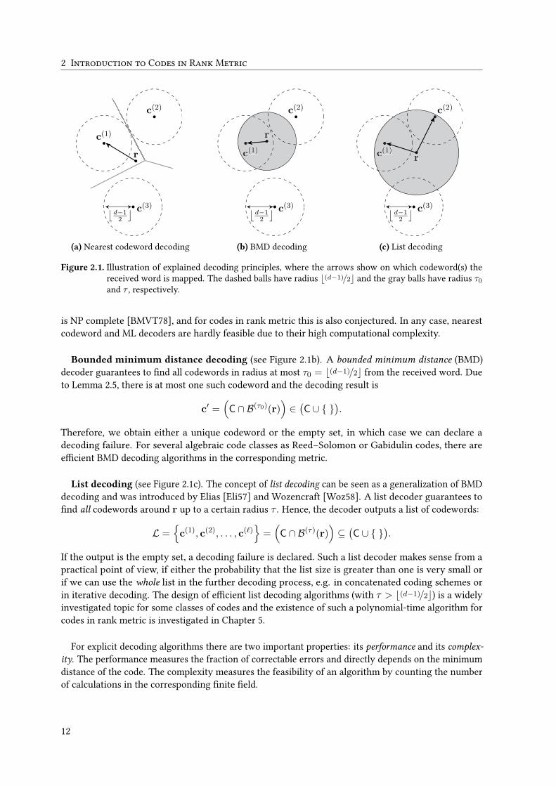


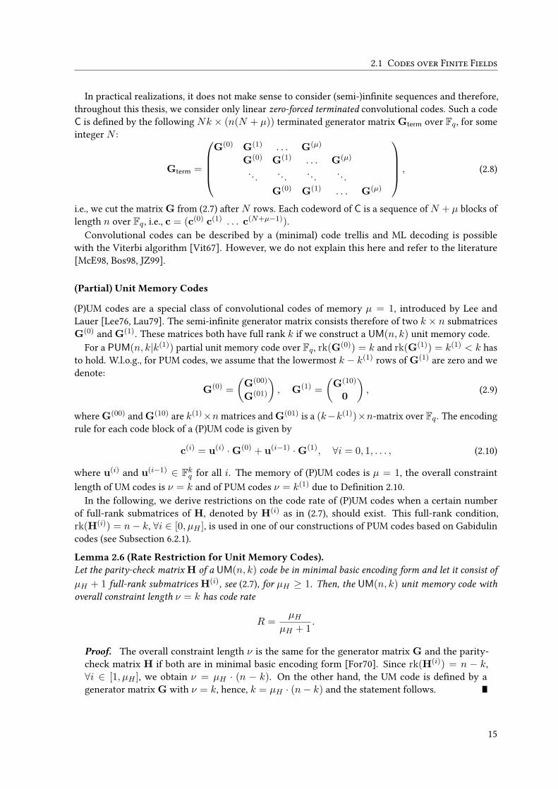

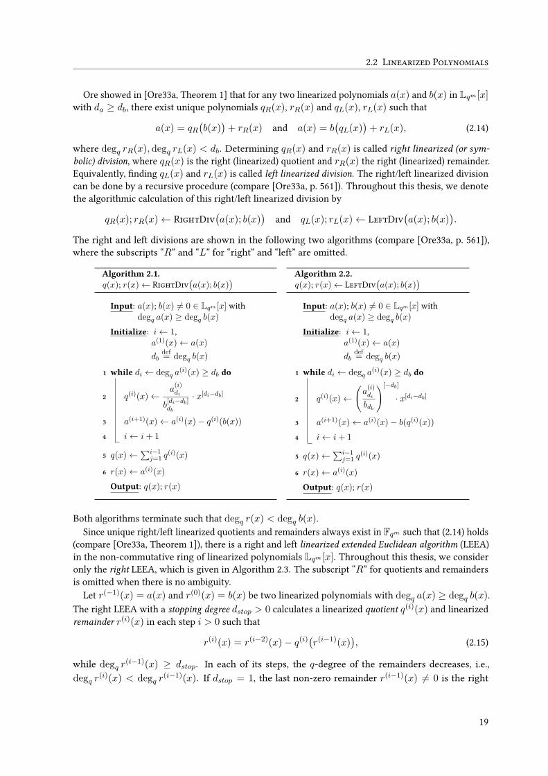
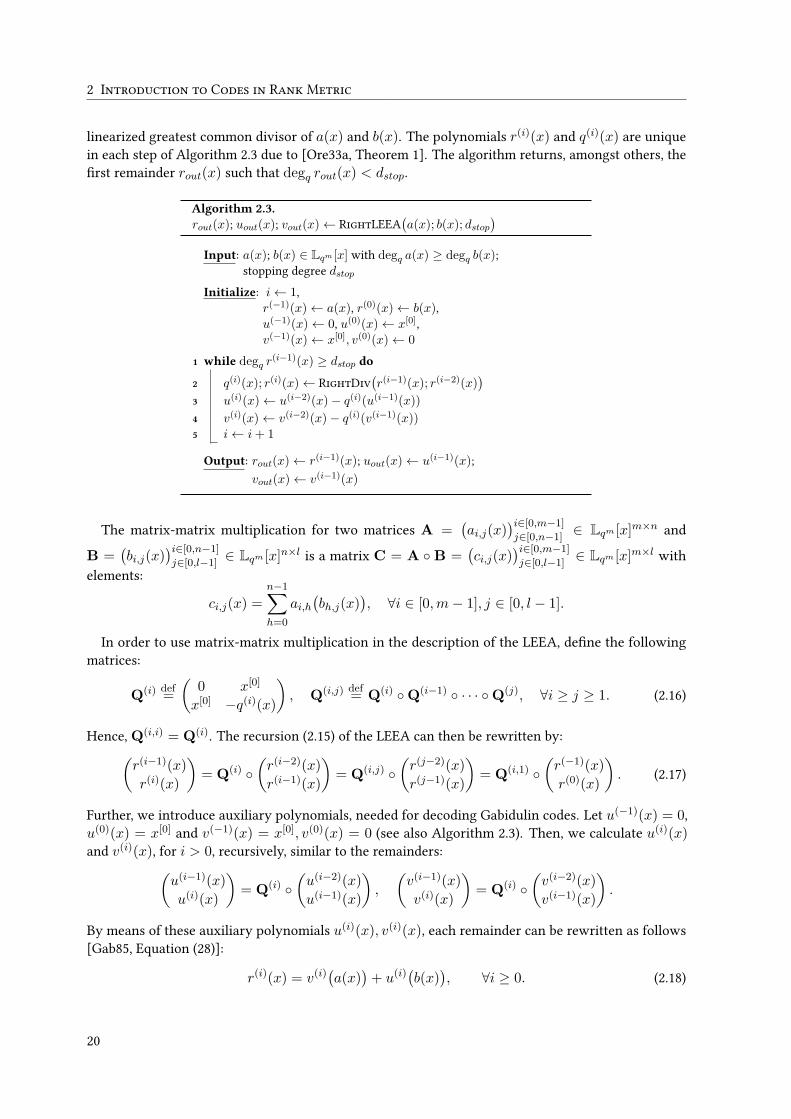


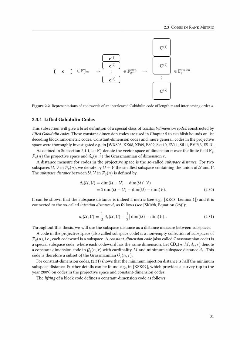

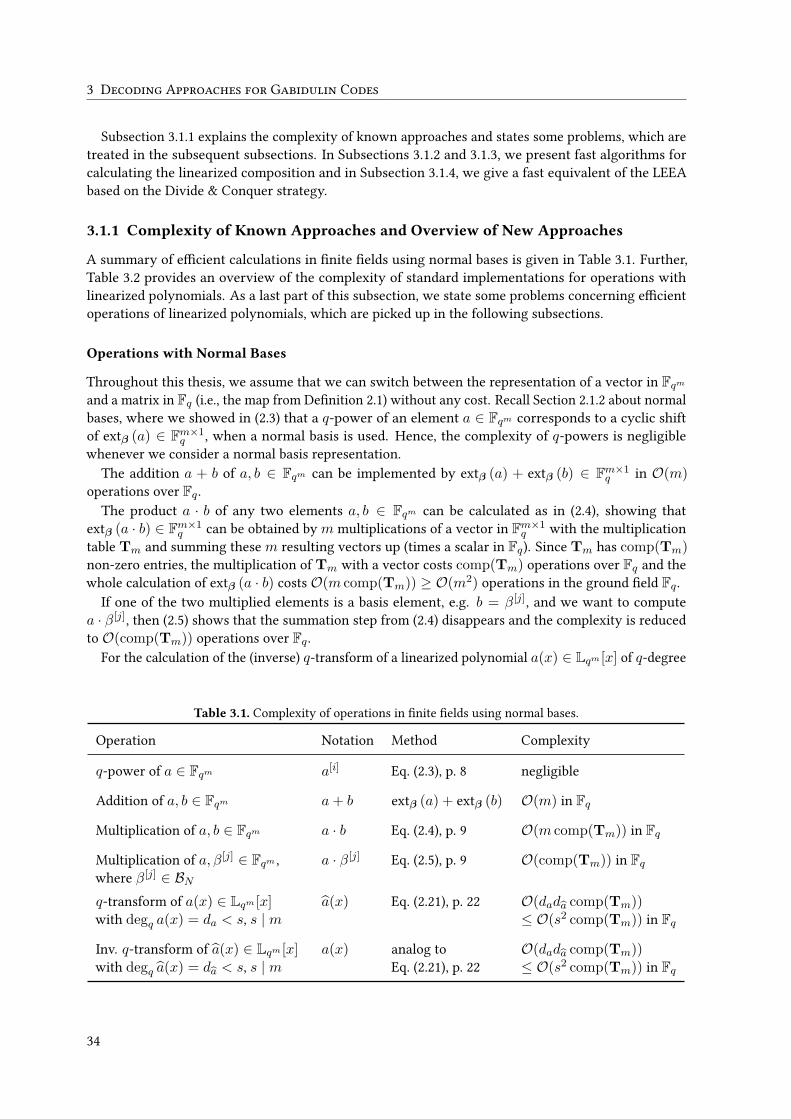
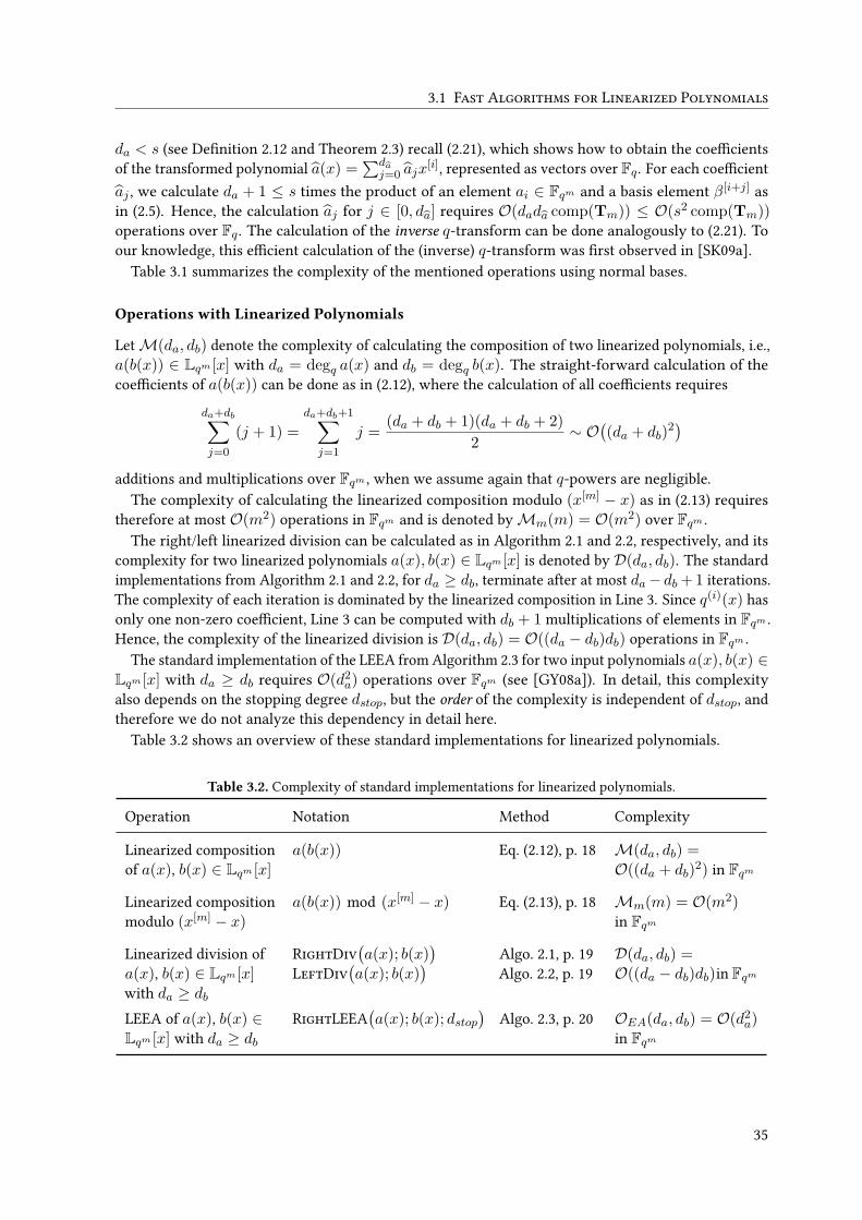
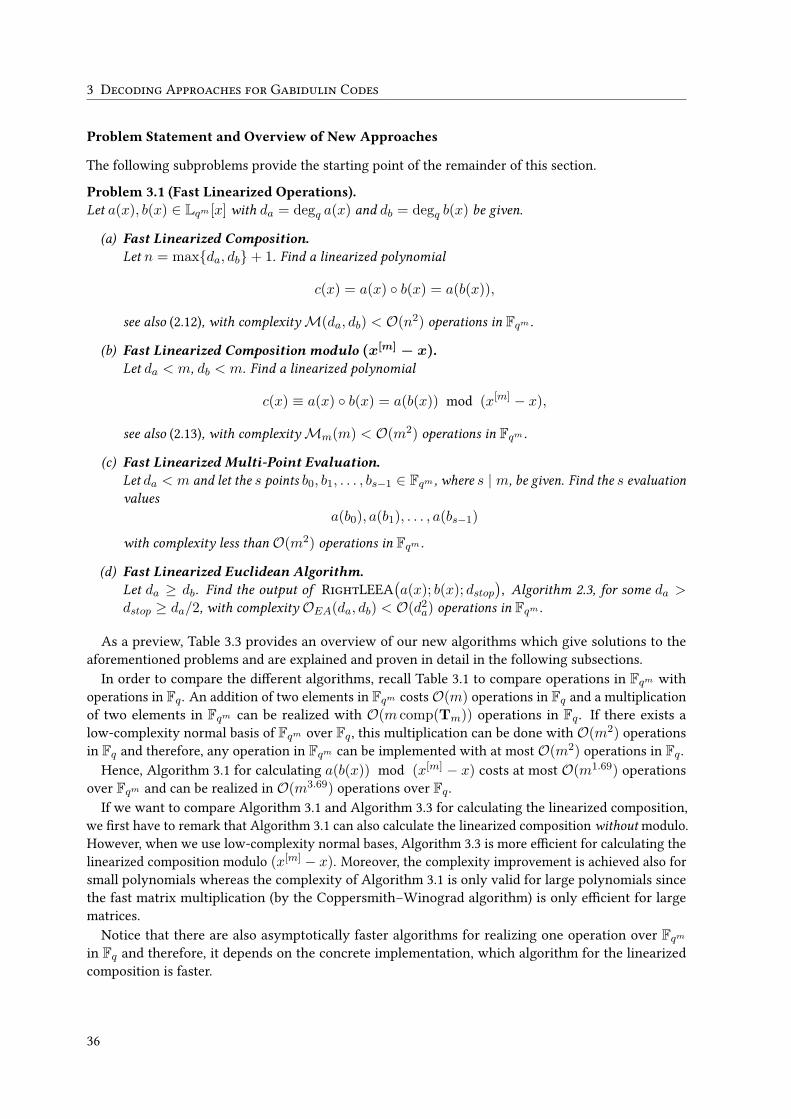
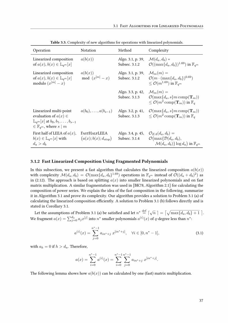


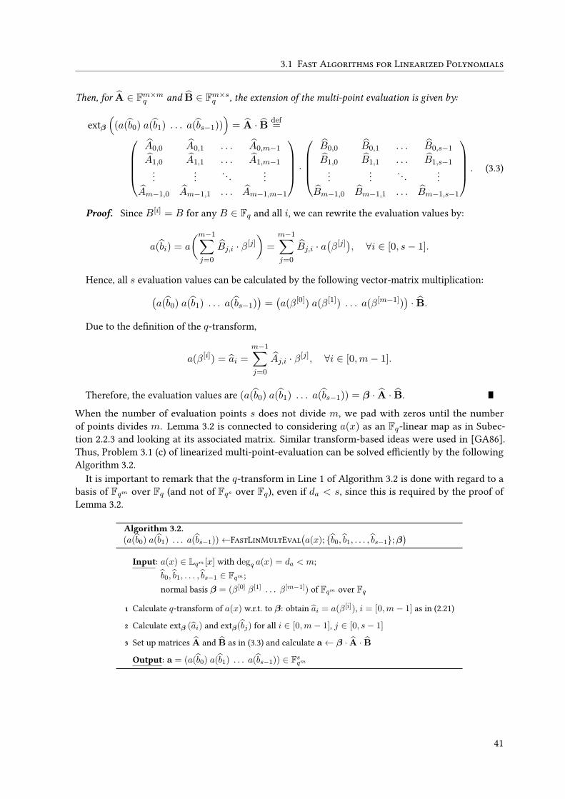


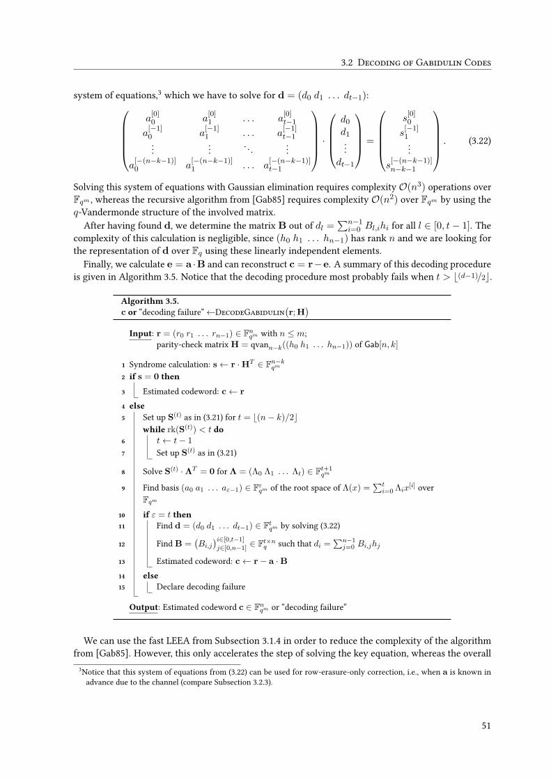
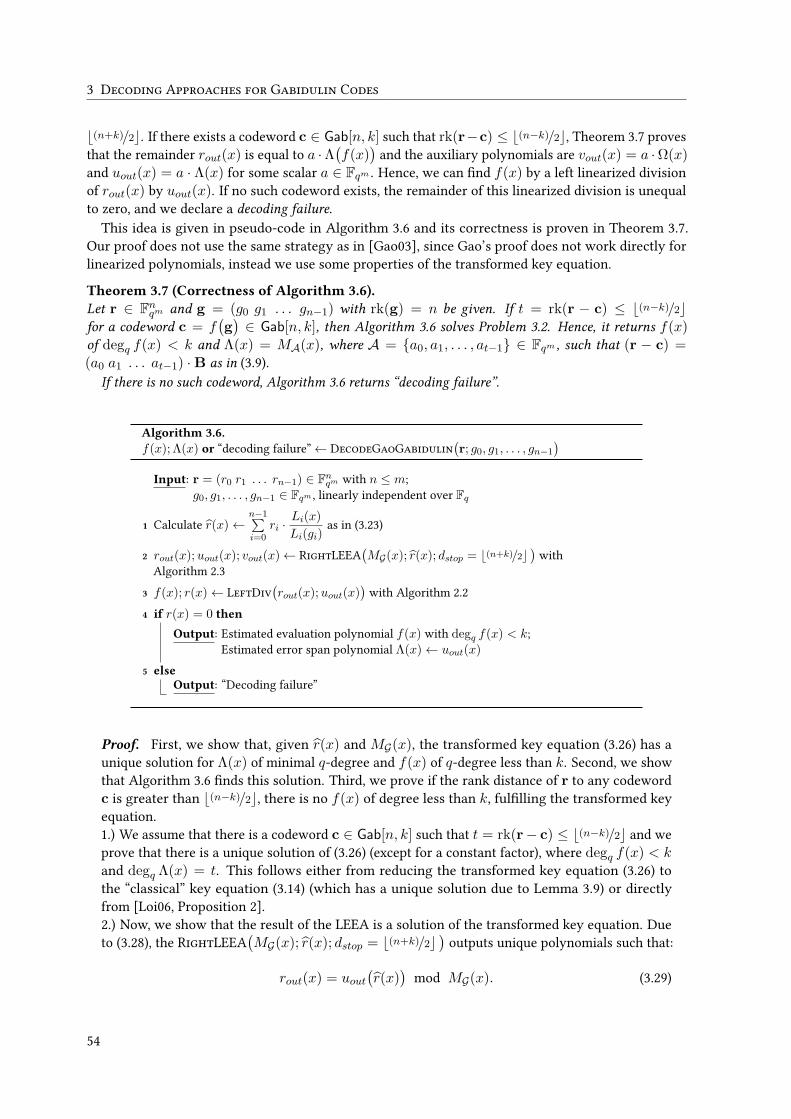


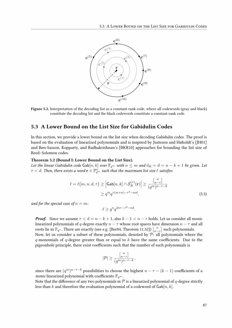

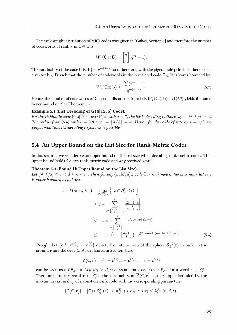


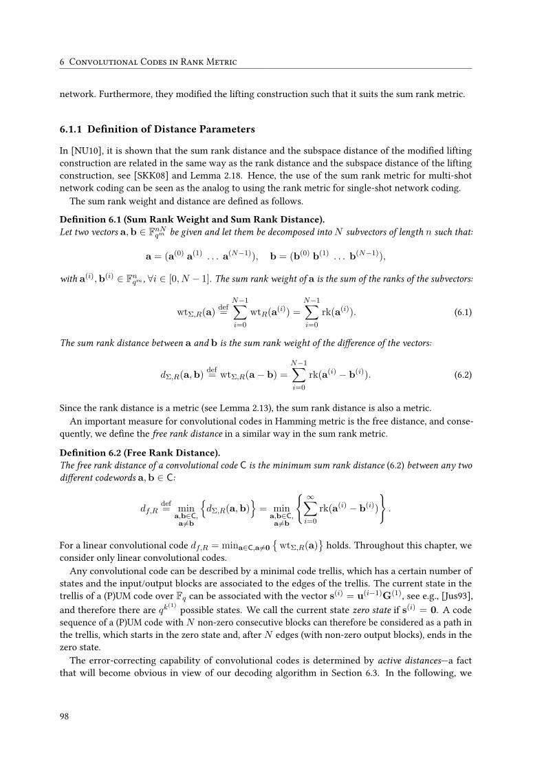
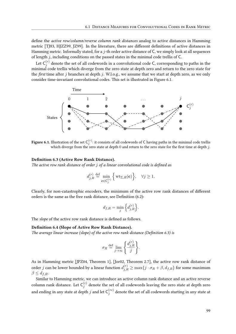
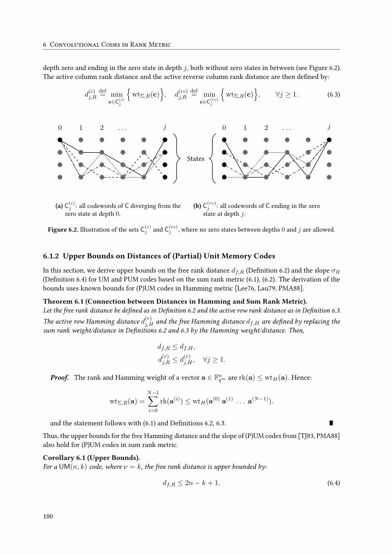


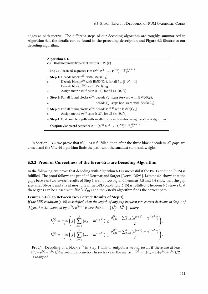


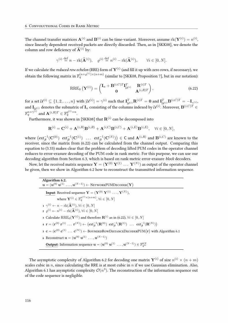
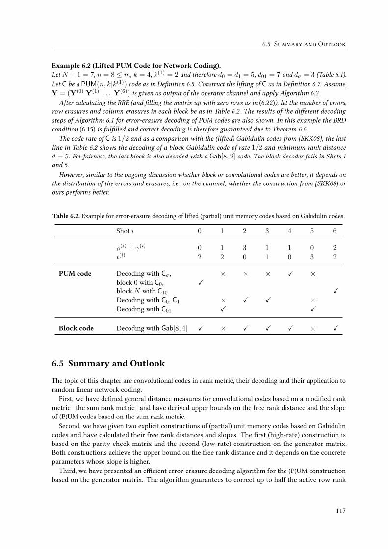


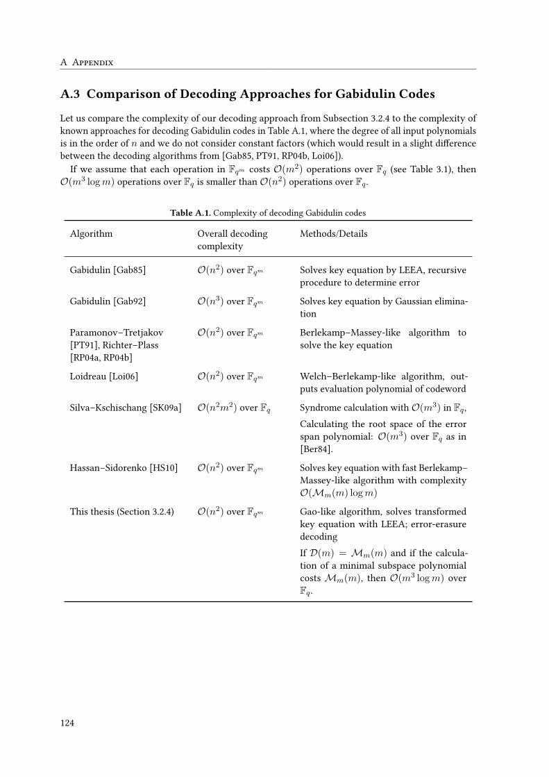


![1 Sequential Decoding of Convolutional Codes - ntpuweb.ntpu.edu.tw/~yshan/book_chapter.pdf · 2 IncontrasttothelimitationoftheViterbialgorithm,sequentialdecodingisrenowned foritscomputationalcomplexitybeingindependentofthecodeconstraintlength[1].](https://static.documents.pub/doc/80x56/5e08b7acda112278e327d004/1-sequential-decoding-of-convolutional-codes-yshanbookchapterpdf-2-incontrasttothelimitationoftheviterbialgorithmsequentialdecodingisrenowned.jpg)


