Introduction LFM Data & Instruments Results Conclusion Appendix Decomposing Local Fiscal Multipliers: Evidence from Japan Taisuke Kameda, Ryoichi Namba, and Takayuki Tsuruga Cabinet Secretariat, CRISER, and Kyoto Univ. August, 2017
Transcript
Introduction LFM Data & Instruments Results Conclusion Appendix
Decomposing Local Fiscal Multipliers:Evidence from Japan
Taisuke Kameda, Ryoichi Namba, and Takayuki Tsuruga
Cabinet Secretariat, CRISER, and Kyoto Univ.
August, 2017
Introduction LFM Data & Instruments Results Conclusion Appendix
Motivation: Fiscal multipliers
� Growing interest in the interaction btwn gov�t spending andthe economic activity
� Fiscal multipliers
� By how many % does output increase when gov�t spendingincreases by 1% of output?
� Two directions in research on �scal multiplier
1. Traditional national �scal multiplier
� Identi�ed from time-series variations
2. Local �scal multiplier (LFM)
� Identi�ed from the region�time speci�c variations
Introduction LFM Data & Instruments Results Conclusion Appendix
Motivation: Local �scal multipliers
� What is the LFM?
� Typical estimation eqn.
Yr ,t � Yr ,t�1Yr ,t�1
= βGr ,t � Gr ,t�1Yr ,t�1
+ αr + δt + εr ,t
Yr ,t : per capita output in region r , Gr ,t : per capita gov�tspending in region r , αr :entity �xed e¤ect, δt : time �xed e¤ect
� The LFM di¤ers from the national �scal multiplier
� b/c δt controls for all common e¤ects of agg. shocks andpolicy (e.g., common e¤ect of monetary policy)
� but β fails to capture common e¤ects of �scal policy
Introduction LFM Data & Instruments Results Conclusion Appendix
Motivation: Spillover
� Another important di¤erence from the national �scalmultiplier
� An interpretation
� Fiscal multiplier of gov�t spending in an economy in amonetary union (e.g., EU countries)
� Within a single country, ...
� Strong interdependence without the border e¤ect
� Gov�t spending may easily spill over into other economies
Introduction LFM Data & Instruments Results Conclusion Appendix
Research questions1. How large is the LFM in Japan?
� We provide estimates of LFM, comparable to other countries
2. How large is the spillover within the region?
� Positive if there is a leakage in demand
� Negative if production factors (e.g., labor) relocate acrossprefectures
3. How large is the LFM on expenditure components of GDP?
� Crowding-out or crowding-in?
� Spillover in expenditure components
Introduction LFM Data & Instruments Results Conclusion Appendix
This paper
1. Estimate LFM at regional level
� Separate the country into regions
� Regional �scal multiplier (RFM)
2. Decompose RFM into prefectural �scal multiplier (PFM) andregion-wide spillover
RFM ' PFM + Region-wide spillover
3. Decompose RFM into expenditure components
RFM ' RFMC + RFMI + RFMG + RFMNX
Introduction LFM Data & Instruments Results Conclusion Appendix
Regions
� De�nition of �Region�used in Prefectural Accounts Estimation
Introduction LFM Data & Instruments Results Conclusion Appendix
Why Japan?
� Prefectural accounts in JPN are constructed in a way highlycomparable to the national account
� Cabinet O¢ ce in JPN publishes C , I , G and NX at theprefectural level
� BEA in the US does not publish I , G and NX at thestate/county level
Introduction LFM Data & Instruments Results Conclusion Appendix
Main �ndings
� RFM = 1.55
Introduction LFM Data & Instruments Results Conclusion Appendix
Main �ndings
� RFM = 1.55
Introduction LFM Data & Instruments Results Conclusion Appendix
Literature on local �scal multipliers
� Most studies are based on the US state/county
� ARRA papers estimate �Jobs-multiplier� and �cost-per-job�� using state-level employment data of BLS� Chorodow-Reich et al. (2012), Conley and Dupor (2013),Wilson (2012), Dupor and McCroy (2017) among others
� Non-ARRA papers focus on output multiplier or incomemultipliers
� Nakamura and Steinsson (2014), Clemens and Miran (2012),Shoag (2016), Suárez-Serrato and Wingender (2016)
� International evidence
� Japan: Brückner and Tuladhar (2014) focus on the 1990s andrelationship with �nancial distress
� Italy: Acconcia et al. (2014), China: Guo et al. (2016)
� Our focus: spillover and expenditure components
Introduction LFM Data & Instruments Results Conclusion Appendix
Empirical strategy
Introduction LFM Data & Instruments Results Conclusion Appendix
Estimation equation used in the literature� Typical estimation eq.
Yr ,t � Yr ,t�2Yr ,t�2
= βRGr ,t � Gr ,t�2Yr ,t�2
+ αr + δt + εr ,tABCDE
� Yr ,t : per capita GDP in region r
� Gr ,t : per capita gov�t spending in region r
� βR : (two-year cumulative) RFM region
� We do not estimate this equation, but ...
Introduction LFM Data & Instruments Results Conclusion Appendix
Our estimation equation� We use the prefecture data...
yr ,p,t � yr ,p,t�2yr ,p,t�2
= γPgr ,p,t � gr ,p,t�2
yr ,p,t�2+ γS
Gr ,t � Gr ,t�2Yr ,t�2
+ηr ,p + δt + εr ,p,t
� yr ,p,t : per capita GDP in prefecture p that belongs to region r
� gr ,p,t : per capita gov�t spending in p
� ηr ,p : entity �xed e¤ect
� An interpretation
� γP : PFM
� γS : region-wide spillover
Introduction LFM Data & Instruments Results Conclusion Appendix
Our estimation equation� ... together with regional gov�t spending:
yr ,p,t � yr ,p,t�2yr ,p,t�2
= γPgr ,p,t � gr ,p,t�2
yr ,p,t�2+ γS
Gr ,t � Gr ,t�2Yr ,t�2
+ηr ,p + δt + εr ,p,t
� yr ,p,t : per capita GDP in prefecture p that belongs to region r
� gr ,p,t : per capita gov�t spending in p
� ηr ,p : entity �xed e¤ect
� An interpretation
� γP : PFM
� γS : region-wide spillover
Introduction LFM Data & Instruments Results Conclusion Appendix
Geographic decomposition� Take the weighted average of estimation eq.
) Yr ,t � Yr ,t�2Yr ,t�2
' (γP + γS )| {z }βR
Gr ,t � Gr ,t�2Yr ,t�2
+ αr + δt + εr ,t
� Weight ωr ,p : time-series mean of the GDP share of p to r
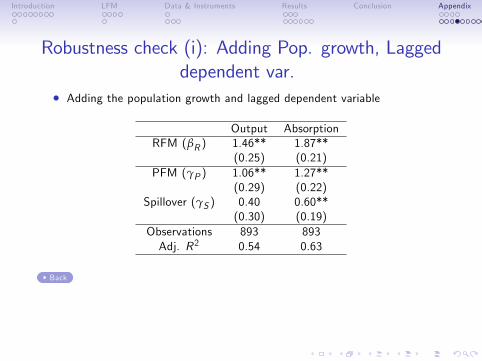
Note: *5% signi�cance level, ** 1% signi�cance level. Time FE and Prefectural FE are included. SE clustered byprefectures. Angrist-Pischke�s �rst-stage F is 17.9 for
�gr ,p,t � gr ,p,t�2
�/yr ,p,t (Adj. R2 = 0.69) and 763.4 for
(Gr ,t � Gr ,t�2 ) /Yr ,t (Adj. R2 = 0.86). We include the dummy for Great East Japan Earthquake as a control
variable.
� In 2SLS
� The estimated RFM is larger than one
� Positive spillover, but imprecisely estimated
Introduction LFM Data & Instruments Results Conclusion Appendix
Expenditure components in GDP
� RFM =1.55
� Crowding-in e¤ect must be observed
� What expenditure components?
Introduction LFM Data & Instruments Results Conclusion Appendix
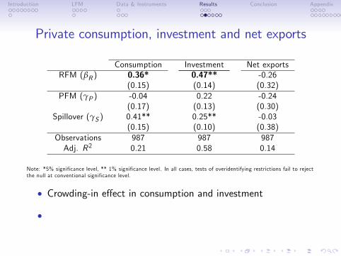
Private consumption, investment and net exports
Consumption Investment Net exportsRFM (βR ) 0.36* 0.47** -0.26
Note: *5% signi�cance level, ** 1% signi�cance level. In all cases, tests of overidentifying restrictions fail to rejectthe null at conventional signi�cance level.
� Crowding-in e¤ect in consumption and investment
� Spillover is economically and statistically signi�cant inconsumption and investment
Introduction LFM Data & Instruments Results Conclusion Appendix
Private consumption, investment and net exports
Consumption Investment Net exportsRFM (βR ) 0.36* 0.47** -0.26
Note: *5% signi�cance level, ** 1% signi�cance level. In all cases, tests of overidentifying restrictions fail to rejectthe null at conventional signi�cance level.
� Crowding-in e¤ect in consumption and investment
� Spillover is economically and statistically signi�cant inconsumption and investment More
Introduction LFM Data & Instruments Results Conclusion Appendix
� We also use regional dummies interacted with ∆Sr ,t and∆Sr ,t�1 to allow for variation in sensitivity to regional variablesacross regions (Nakamura and Steinsson 2014)
Introduction LFM Data & Instruments Results Conclusion Appendix
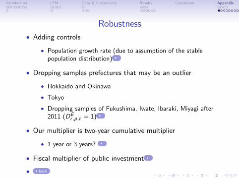
Control variables� In benchmark regression, we control for the negative impactof Great East Japan Earthquake
� Dummy DEr ,p,t that takes one if the prefecture are stronglyin�uenced by the earthquake and year t > 2011
DEr ,p,t =�1 if Fukushima, Ibaraki, Iwate, Miyagi and t > 20110 otherwise.
� Local tax rate?
� We did not control for local tax rate, b/c local tax ratesalmost fully comove over time