1

Decomposition of Complex Line Drawings withHidden Lines for 3D Planar-Faced Manifold

Object ReconstructionJianzhuang Liu, Senior Member, IEEE, Yu Chen, Student Member, IEEE, and Xiaoou Tang, Fellow, IEEE

✦

Abstract —3D object reconstruction from a single 2D line drawing isan important problem in computer vision. Many methods have beenpresented to solve this problem, but they usually fail when the geometricstructure of a 3D object becomes complex. In this paper, a novelapproach based on a divide-and-conquer strategy is proposed to handlethe 3D reconstruction of a planar-faced complex manifold object fromits 2D line drawing with hidden lines visible. The approach consistsof four steps: 1) identifying the internal faces of the line drawing, 2)decomposing the line drawing into multiple simpler ones based on theinternal faces, 3) reconstructing the 3D shapes from these simpler linedrawings, and 4) merging the 3D shapes into one complete objectrepresented by the original line drawing. A number of examples areprovided to show that our approach can handle 3D reconstruction ofmore complex objects than previous methods.

Index Terms —3D reconstruction, divide and conquer, internal face, linedrawing, manifold.

1 INTRODUCTION AND RELATED WORK

A line drawing is the 2D projection of the wireframe ofan object. Humans have no difficulty in perceiving the3D geometry from a 2D line drawing. Emulating thisability is an important research topic in both computervision and graphics. Line drawings discussed in thispaper are with hidden lines visible. These line drawingscan be generated by sketching on the screen with amouse or a tablet PC pen and on paper with a pen.Though it takes more effort for the user to draw suchline drawings, compared with line drawings withouthidden lines, they allow the reconstruction of completeand more complex objects. Much work concerning linedrawings with hidden lines has been published in thecomputer vision literature [1], [2], [3], [4], [5], [6], [7], [8],[9], [10], [11], [12], and in CAD and graphics [13], [14],[15], [16], [17], [18], [19], [20], [21]. The applications of 3Dreconstruction from this kind of line drawings include: 1)providing a flexible sketching interface in current CADsystems [14], [16], [18], 2) providing a 2D sketch queryinterface for 3D object retrieval from large databases orfrom the internet [19], [22], [23], 3) interactive generation

The authors are with the Department of Information Engineering, TheChinese University of Hong Kong, Hong Kong. Emails: {jzliu, ychen6,xtang}@ie.cuhk.edu.hk

of 3D models from images [9], [17], [20], 4) automaticconversion of existing industrial wireframe models tosolid model [13], [14], and 5) building rich databasesfor object recognition systems and reverse engineeringalgorithms for shape reasoning [13], [14].

The earliest work towards 3D reconstruction fromsingle line drawings is line labeling, which focuses onfinding a set of consistent labels from a line drawingto test the correctness and/or realizability of the linedrawing [3], [4], [5], [16], [24], [25], [26], [27], [28], [29],but it does not explicitly recover a 3D object from aline drawing. Most 3D reconstruction methods from aline drawing assume that the face topology of the linedrawing is known in advance. This information cangreatly reduce the complexity of the reconstruction. Faceidentification is not a trivial problem, and many methodshave been proposed to find faces from a line drawing [1],[6], [7], [8], [12], [13], [14], [30].

3D reconstruction from line drawings is usually for-mulated as an optimization problem. Marill proposeda criterion of minimizing the standard deviation of theangles in the reconstructed object so that a 2D linedrawing can be inflated into a 3D shape [2]. Later,more criteria, such as line parallelism, face planarity,object symmetry, and so on, were proposed to do 3Dreconstruction [1], [9], [11], [15], [18], [20], [21], [31],[32], [33]. The methods in [26], [34], and [35] use linelabeling and shading information to recover the visiblesurfaces of 3D polyhedra in images from the edgesof these polyhedra. Recently, some attempts [32], [33],[36] were made to recover a complete solid from a linedrawing with visible lines only, but these methods areonly applicable to simple objects. Almost all previouswork on 3D reconstruction from line drawings focuseson planar-faced objects.

In previous optimization-based methods, the variablesof the objective functions are the missing depths of thevertices of a line drawing. These methods work well forsimple objects with a small number N of the variables.As N grows, however, it is very difficult for them tofind expected objects. This is because with the nonlinearobjective functions in a space of large dimension N , the

2

search for optimal solutions can easily get trapped intolocal minima. To handle this problem, Liu et al. proposedto find much lower dimensional search spaces wheredesired objects can be found more easily [9]. This methodcan tackle 3D reconstruction of more complex objectsthan previous methods. From [9], we know that the size(dimension) of the search space depends on the degree ofreconstruction freedom (DRF) of a line drawing, and theDRF usually increases when the number of the internalfaces (see the next section for its definition) of the objectincreases. In a high dimensional space, the search fordesired objects become difficult [9]. Our experimentsshow that the algorithm in [9] still often fails to obtainan expected 3D object from a line drawing when thegeometry of the object becomes more complex withmany faces and internal faces.

In this paper, we propose a divide-and-conquer strat-egy to handle the 3D reconstruction of complex planar-faced manifold objects from line drawings, which isthe comprehensive version of our preliminary workpublished in [10]. In addition to the contents in [10],we discuss how to find internal faces, prove the exis-tence and uniqueness of the partition of a line drawingalong an internal face, and provide more experiments.Manifolds belong to a class of most common solids, thedefinition of which is given in the next section. Thisapproach is based on the fact that a complex object1 isin general the combination of less complex objects, eachof which is easier to recover. Fig. 1 shows an examplewhere a line drawing is decomposed into four simplerones. Obviously, the 3D reconstruction from each ofthem is an easier task than the reconstruction from theoriginal line drawing. Our approach includes four steps:1) identifying the internal faces of an input line drawing,2) decomposing the line drawing into less complex onesbased on the internal faces, 3) reconstructing the 3Dshape from each of these simpler line drawings, and 4)merging these 3D shapes into a complete object.

The rest of this paper is organized as follows. Section 2states the assumptions for the reconstruction problemand defines terms that are frequently used in the paper.In Section 3, we propose our method for the decom-position of a complex line drawing into simpler ones.Section 4 presents the reconstruction algorithm for merg-ing the 3D objects that are recovered from the simplerline drawings. Our experimental results are shown inSection 5, and finally Section 6 concludes the paper.

2 ASSUMPTIONS AND TERMINOLOGY

In this paper, we focus on a class of common solids,called manifolds, with planar faces. A line drawing, rep-resented by a single edge-vertex graph with the known xand y coordinates of the vertices, is the parallel or near-parallel projection of the edges of a manifold in a generic

1. The complexity of an object is an ambiguous term. In this paper,we say that a manifold object is complex if it has both more than 30faces and non-trihedral vertices, which causes internal faces or holes.

(a) (b)

1

2

8

7

9

6 13

5 3

15

11

16

12

14 17

10

4

*

1 f

*

2 f

*

3 f

*

4 f

7

9

6

11

Fig. 1. Decomposition of a line drawing and illustration of some terms.(a) Cycle (1, 3, 4, 1) is a real face. The four shadowed cycles f∗1−4are internal faces. Edges {10, 16} and {8, 14} are two artificial linesindicating the coplanarity of cycles (6, 7, 9, 11, 6) and (12, 13, 15, 17, 12).Edge {1, 2} is a chord of cycle (1, 5, 2, 3, 1). Two real faces (1, 3, 4, 1)and (1, 2, 5, 1) are connected. Edge {5, 4} and the real face (1, 3, 4, 1)are connected. (b) Four simpler line drawings are decomposed from thefour internal faces f∗1−4 in (a).

view where all the edges and vertices of the manifoldare visible. The generic view assumption means that thetopology of the line drawing is preserved under smallvariations of the viewpoint, which is the assumptionmade in most previous related work. We also assumethat all the faces of the manifold have been identifiedfrom its input line drawing. Face identification from linedrawings with hidden lines visible has been studiedextensively [1], [6], [7], [8], [12], [13], [14], [30], and thealgorithms developed in [7] and [30] can be used to findthe faces from a line drawing. For better understandingthe content in the following sections, we here summarizethe terms that appear in the rest of the paper. Many ofthem are illustrated with the line drawings in Fig. 1.

• Manifold. A manifold, or more rigorously 2-manifold, is a solid where every point on its surfacehas a neighborhood topologically equivalent to anopen disk in the 2D Euclidean space [37]. This paperconsiders such manifolds that are made up of flatsurfaces. A basic property of a manifold is that eachedge is shared by exactly two faces [38].

• Face (real face). A face is one of the flat surfacesthat make up a manifold. In what follows, We callit a real face to distinguish it from an internal face.

• Internal face. An internal face is an imaginary facelying entirely inside a manifold M with only itsedges visible on the surface. It is not a real face, butcan be considered as two coincident real faces ofidentical shape belonging to two manifolds or twoparts of the same manifold which have been gluedtogether to build M .

• Edge. An edge of a line drawing is the intersectionof two non-coplanar real faces. An edge e is alsodenoted by {ve1, ve2} where ve1 and ve2 are twovertices of e.

• Artificial line. An artificial line is a line used toindicate the coplanar relationship of two cycles.

3

• Cycle. A cycle is formed by a sequence of verticesv0, v1, · · · , vn, where n ≥ 3, v0 = vn, the n verticesare distinct, and there exists an edge connecting vi

and vi+1 for i = 0, 1, · · · , n − 1. A cycle is denotedby (v0, v1, · · · , vn). Since the boundary of a face is acycle, a face is denoted the same way as a cycle.

• Chord. A chord of a cycle is an edge that connectstwo nonadjacent vertices of the cycle.

• Vertex set of a cycle. The vertex set V er(C) of acycle C is the set of all the vertices of C.

• Edge set of a cycle. The edge set Edge(C) of a cycleC is the set of all the edges of C.

• Connected faces. Two faces fa and fb are calledconnected if V er(fa) ∩ V er(fb) 6= ∅.

• Connected edge and face. An edge e = {ve1, ve2} iscalled connected to a face f if {ve1, ve2}∩V er(f) 6= ∅and e /∈ Edge(f).

• Partition of a set. Given a non-empty set S, apartition PS = {S1, S2} is a set of two non-emptysubsets S1 and S2 of S such that S1 ∪ S2 = S andS1 ∩ S2 = ∅.

An internal face is where two separate manifolds (ortwo parts of one manifold) are glued together. It may benon-planar. However, we treat all the internal faces asplanar in this paper, which is true for most manifoldswith internal faces. The advantage of this treatment isthat when an object is separated along an internal face,this internal face becomes a real planar face, and thedecomposed line drawings still represent planar-facedmanifolds.

3 DECOMPOSITION OF A L INE DRAWING

There are many ways to separate the edge-vertex graphof a line drawing into multiple smaller graphs. However,these graphs are meaningless if they do not representreal objects. Obviously, it is desirable that each of theseparated line drawings still represents a manifold. Wehave this as a requirement to design our method forline drawing decomposition. By observing numerouscomplex objects, especially man-made objects, we cansee that most of them are formed by gluing two ormore smaller objects together, resulting in internal faces.Therefore, our strategy is to find the internal faces froma line drawing first and then decompose it along theinternal faces.

3.1 Classification of Internal Faces

Let an internal face f∗ be generated by gluing tworeal faces f1 and f2. Let C1 and C2 be the two cyclescorresponding to f1 and f2, respectively, in the originalline drawing. We can classify f∗ into one of the twotypes: 1) C1 and C2 have no contact, and 2) C1 and C2

have contact (partly or completely). Fig. 1(a) shows fourexamples of internal faces, in which f∗1 belongs to type 1,and f∗2 , f∗3 , and f∗4 belong to type 2. For f∗4 , C1 and C2

merge into one in the line drawing.

v

c v

a v b

v 1

f

2 f 3

f

Fig. 2. Part of a line drawing with an artificial line {v, vc}.

3.2 Decomposition along Internal Faces of Type 1

When f∗ belongs to type 1, since C1 and C2 do nottouch, additional information must be used to indicatethe coplanarity of C1 and C2 so that correct face iden-tification and reconstruction from the line drawing arepossible. Using artificial lines to indicate this coplanarityis the simplest and most straightforward way, which hasbeen used in solid modeling [7], [13]. Two artificial linesconnecting two edges of C1 to two edges of C2 are addedby the user who designs the line drawing. Note that ingeneral, one artificial line is not enough to indicate thecoplanarity because each edge is shared by two real facesin a manifold.

For an internal face of type 1, if we can detect thetwo artificial lines, then we can remove them and thusdecompose the line drawing along this internal face. Infact, the detection of artificial lines are not difficult asdescribed below.

Let {v, va}, {v, vb}, and {v, vc} be the three edgesconnected to a vertex v of degree 3, as shown in Fig. 2. If{v, va} and {v, vb} are collinear, then {v, vc} is an artificialline. This statement is easy to verify.

Assume, on the contrary, that {v, vc} is not an artificialline but an edge. Since the line drawing denotes amanifold, every edge is passed through by two real facesand hence three real faces f1, f2, and f3 pass through v(see Fig. 2). According to the assumption that the linedrawing is the projection of a manifold in a genericview, the three vertices va, v, and vb are also collinearin 3D space. Thus, the straight line vavvb and vertexvc define a plane in 3D space, implying that f2 andf3 are coplanar, which contradicts the definition that anedge is the intersection of two non-coplanar real faces.Therefore, {v, vc} is an artificial line.

After artificial lines are detected, they are removedfrom the line drawing. Note that when an artificial lineis removed, its two vertices in the original line drawingare also removed. For example, when the artificial line{10, 16} in Fig. 1(a) is removed, the two collinear edges{11, 10} and {10, 9} become one edge {11, 9}. An internalface of type 1 turns out to be a real face in the decom-posed line drawing. The face (6, 7, 9, 11, 6) in Fig. 1(b) issuch an example.

3.3 Detecting Internal Faces of Type 2

Even with the real faces known from a line drawing,detecting internal faces of type 2 is not a trivial problem.

4

a

b d

c

b

a

f e

d

c

f g

e

1 C

2 C

(a) (b)

Fig. 3. (a) A cycle C1 = (f, a, b, ..., c, d, e, ...f) with a chord{a, d} enclosed completely by C1. (b) Another cycle C2 =(f, a, b, ..., c, e, d, g, ...f) with a chord {a, d} enclosed partially by C2.

In this paper, the detection is performed through acycle-searching scheme. Since exhaustive searching iscomputationally expensive, we here develop propertiesrelated to internal faces of type 2 so that most cycles thatcannot be such an internal face can be eliminated duringthe search.

In the rest of Section 3, we only consider internalfaces of type 2. For concision, we simply use “internalface(s)” to denote “internal face(s) of type 2”. When wesay two cycles overlap, we mean that their enclosedregions overlap on the 2D line drawing plane. Thefirst two properties below come from the definition andobservation of common internal faces. They are usefulto develop other subsequent properties. The assumptionthat all internal faces are planar is also implied.

Property 1: An internal face except its boundary isinvisible from any viewpoint.

Property 2: Two coplanar internal faces do not overlap.Property 3: A self-intersecting cycle is not an internal

face.Proof: Since the projection of the boundary of a

planar face cannot form a self-intersecting cycle [7], aninternal face, which is formed by gluing the real faces oftwo planar manifolds, cannot be self-intersecting either.

Property 4: If two cycles share two or more non-collinear edges and overlap, then they cannot both beinternal faces.

Proof: Since the two cycles share two or more non-collinear edges, they must be coplanar if they are internalfaces. From Property 2, they cannot both be internalfaces.

Property 5: A cycle cannot be an internal face if thecycle has a chord that is completely or partially enclosedinside the cycle.

Proof: If this cycle is an internal face (see Fig. 3),the chord is obviously on the same plane with the cycle.An edge of a line drawing lies on the surface of themanifold and is visible from a certain viewpoint in 3Dspace. Hence, it causes an interior part of the internalface to be visible, which contradicts Property 1.

Property 6: A cycle cannot be an internal face if thiscycle and a real face share two or more non-collinearedges and they have an overlapping region.

Proof: If this cycle is an internal face and shares twoor more non-collinear edges with a real face, then the

f

C

(a) (b)

f

C f

C

f

C

(c) (d)

Fig. 4. Several cases where a cycle C and a real face f share twonon-collinear edges and they have an overlapping region in the linedrawing. (a) C and f have intersecting edges. (b)–(d) C and f havean overlapping region without intersecting edges.

C b

1 f 2

f a

C

1 f 2

f

(a) (b)

Fig. 5. A cycle C sharing two non-collinear edges with two real facesf1 and f2. (a) f1 and f2 having a common edge {a, b}. (b) f1 and f2

overlapping.

cycle and the real face lie on the same plane. If theyfurther have an overlapping region in the line drawing,then this region is visible, which contradicts Property 1.

Property 7: A cycle cannot be an internal face if this cy-cle and a real face share two or more non-collinear edgesand they have edges intersecting in the line drawing.

Proof: If this cycle is an internal face and shares twoor more non-collinear edges with a real face, then thecycle and the real face lie on the same plane. If theyfurther have intersecting edges, then part of the real facemust be enclosed by the internal face, which contradictsProperty 1.

Fig. 4 shows several cases where a cycle and a real faceshare two non-collinear edges and they have an over-lapping region in the line drawing. In fact, Property 7is a special case of Property 6. It is stated explicitly asa separate property because it can be used to reducefruitless search for internal faces before a path becomesa cycle. For other cases such as Figs. 4(b)–(d) where thecycle and the real face have no intersecting edges, thecycle can be determined not to be an internal face afterthe cycle is formed.

Property 8: A cycle cannot be an internal face if 1) thiscycle shares two or more non-collinear edges with a realface and shares another two or more non-collinear edgeswith another real face, and 2) the two real faces share anedge or they have an overlapping region.

Proof: Let the cycle, the two real faces be C, f1,and f2, respectively. Assume, on the contrary, that Cis an internal face. From the first condition, we knowthat C, f1, and f2 all lie on the same plane. If f1 andf2 share an edge, as shown in Fig. 5(a), the definitionthat an edge is the intersection of two non-coplanar realfaces is violated. In another case, f1 and f2 overlap, asshown in Fig. 5(b). However, two co-planar real faces

5

1

2

3

4 5

6

7

8

9

10

Fig. 6. An example where multiple solutions exist.

of an manifold must not overlap in the line drawing.Therefore, C cannot be an internal face.

With these properties, we can develop an algorithmto detect the internal faces of a line drawing, which issummarized in Algorithm 1. It is a depth-first searchalgorithm with the properties incorporated to guide thesearch. The properties can cut most fruitless branchesduring the search, and thus considerably speed up thealgorithm.

In the algorithm, an array Path is used to keep thevertices in the current search path; the variable indexgives the position of the last-added vertex in Pathduring the search. A binary label Label(v) is used forevery vertex v to denote whether v is in Path or not.In practical applications, we can often set the maximumlength Dmax of internal faces to avoid fruitless search.Dmax is used with a 2D array Shortest in step 8(a),which indicates the smallest number of edges in a pathbetween any two vertices.

The algorithm starts the search from every edge inthe line drawing (see step 2), and calls the proce-dure INTERNAL recursively to detect possible internalfaces. Obviously, this search does not miss any internalfaces. In addition, all our experiments show that theoutputted cycles are indeed internal faces, which sug-gests that the properties not only speed up the searchbut also effectively distinguish internal faces from othercycles. The complexity of the algorithm depends onthe structure of a line drawing and is exponential inthe worst case. However, our experiments in Section 5indicate that its computational time is acceptable evenfor complex line drawings.

For some line drawings, there exist incompatible in-ternal faces, resulting in multiple solutions from a linedrawing (see step 3 and “Output” in the algorithm). Oneexample is shown in Fig. 6, which has 15 real faces. Fromthis line drawing, Algorithm 1 finds three internal facesC1 = (1, 2, 3, 4, 5, 6, 7, 8, 1), C2 = (1, 2, 3, 4, 5, 8, 1), andC3 = (5, 8, 9, 10, 5). Since C1 and C2 are incompatibleaccording to Property 4, the algorithm finally outputstwo solutions: one is C1 and C3 and the other is C2 andC3. Note that when C1 is an internal face, C1 and thereal face (5, 6, 7, 8, 5) are on the same plane; when C2 isan internal face, C2 and this real face are on differentplanes.

The reader may wonder why C3 in Fig. 6 is also aninternal face. In fact, holes and cavities may also generate

Algorithm 1 Depth-first search of internal faces.Input: An line drawing L = (V, E ,F) where V , E , and Fare the sets of vertices, edges, and real faces, respectively,the adjacency lists AdjList(v) for every vertex v ∈ V ,a 2D array Shortest(v1, v2) indicating the length of theshortest path between any two vertices v1 and v2, andthe maximum search depth Dmax.

1) Initialization: F∗ ← ∅; Label(v) ← 0, for everyvertex v ∈ V ;

2) for every edge {u, v} ∈ E doa) index ← 1; Label(u) ← 1; Label(v) ← 1;b) Path(0) ← v; Path(1) ← u;c) for every vertex w1 ∈ AdjList(u) and w1 6= v

do INTERNAL(u,w1);d) Path(0) ← u; Path(1) ← v;e) for every vertex w2 ∈ AdjList(v) and w2 6= u

do INTERNAL(v, w2);3) Detect if there are incompatible internal faces in F∗

according to Property 4;Output: The set of internal faces in F∗ if there are noincompatible internal faces, or the sets of internal facesif there are incompatible internal faces.procedure INTERNAL(u, v)

4) index ← index + 1; Label(v) ← 1;5) Path(index) ← v;6) Check if edge {u, v} intersects any previous edges

in Path (according to Property 3). If yes, goto 9;7) With the set of real faces that shares two or more

edges with the current path in Path, check ifthis path can form an internal face according toProperties 7 and 8. If no, goto 9;

8) for every vertex w ∈ AdjList(v) and w 6= u doa) if Label(w) = 0 and index +

Shortest(Path(0), w) ≤ Dmax, then extendthe path by calling INTERNAL(v, w);

b) else if w = Path(0) (a cycle is obtained in thiscase) theni) Check if edge {v, w} intersects any pre-

vious edges in Path (according to Prop-erty 3). If yes, goto 9;

ii) With all the chords of the cycle in Path,check if this cycle can form an internal faceaccording to Property 5. If no, goto 9;

iii) With all the real faces, check if this cy-cle can form an internal face according toProperty 6. If no, goto 9;

iv) Put this cycle into F∗ if it is not a real faceand is not in F∗ yet;

9) index ← index− 1; Label(v) ← 0;end of INTERNAL.

6

1 C

(a) (b)

(c) (d)

2 C

=

=

+

Fig. 7. Union and subtraction that generate internal faces. (a) Amanifold. (b) Two manifolds whose union results in the manifold in (a).(c) Another manifold. (d) Two manifolds, with which the subtraction ofthe smaller one from the bigger one results in the manifold in (c). C1

and C2 are two internal faces.

internal faces, but the definition of internal faces needsto be extended a little. Here a hole is one that passesthrough the surface of a manifold while a cavity doesnot. The manifold in Fig. 1 has a hole while the manifoldin Fig. 6 has a cavity. Next we discuss this extension withtwo simple objects in Figs. 7(a) and (c).

In Section 2, we define an internal face as a face insidea manifold only with its edges visible on the surface,and it is formed by gluing two manifolds together. Onesuch example is shown in Fig. 7(a) where C1 (denotedby the bold cycle) is the internal face. Obviously, theobject in Fig. 7(a) can be considered as the union (gluing)of the two smaller objects in Fig. 7(b). In another case,the object shown in Fig. 7(c) can be considered as thesubtraction of the smaller object from the bigger objectshown in Fig. 7(d). Comparing the two line drawings (a)and (c), we can see that they have very similar structuresand the same topology. The region enclosed by C1 isinvisible and is the common part of the two separateobjects in Fig. 7(b). There is also such a region enclosedby C2 (the bold cycle) that is invisible since it is nota real face, and is the common part of the two objectsin Fig. 7(d). Therefore, we also call C2 an internal face.Note that Algorithm 1 also finds it as an internal facebecause Properties 1–8 do not prevent it from being so.Now we see that an internal face can be formed either bygluing two manifolds together or by cutting a manifoldfrom another. On the other hand, it is easy to know thatgluing two manifolds or cutting a manifold from anothermay not necessarily result in an internal face.

The cycle C3 = (5, 8, 9, 10, 5) in Fig. 6 is similar to thecycle C2 in Fig. 7(c). In Fig. 6, since C3 is compatiblewith both C1 and C2 while C1 and C2 are incompatible,Algorithm 1 obtains the two solutions {C1, C3} and{C2, C3}. Both of them are valid but lead to differentdecompositions of the line drawing, which is discussedin the end of the next section.

(a) (b)

b

a c

d

b

c

d

1 a

2 a

(c)

Fig. 8. An example of decomposing a line drawing along its internalfaces. (a) The line drawing with one internal face shadowed. (b) Thecorrect partition along this internal face. (c) Partitions along the fourinternal faces. The hidden edges are shown in dashed for easierobservation.

3.4 Decomposition along Internal Faces of Type 2

From an internal face, we decompose the line drawing byrecovering the two touching faces that form the internalface. Given a line drawing and its identified real andinternal faces, it is not a trivial problem to decomposethe line drawing. The main difficulties are: 1) the 3Dgeometry of the manifold is not available yet; 2) in the2D projection, the lines connecting to an internal face canbe in any direction with respect to the internal face; and3) when a line drawing is decomposed into two sidesalong an internal face, for a line that is connected tothe internal face in the original line drawing, it is notobvious to which side this line should be connected. Forexample, the correct decomposition of the line drawingalong the shadowed internal face in Fig. 8(a) is given inFig. 8(b). If the edge {a, b} is not connected to a1 but toa2, then a wrong decomposition occurs, because the realface (a, b, c, d, a) is broken after such a decomposition.

Through the observation of numerous line drawings,we find that the human decomposition of a line drawingalong an internal face f∗ always satisfies the followingtwo properties:

Property 9: All the real faces connected to f∗ are par-titioned into two sets, F0(f∗) and F1(f∗).

Property 10: Two real faces sharing a common edgeconnected to f∗ (not including any edge of f∗) bothappear in either F0(f∗) or F1(f∗).

These two properties are easy to verify based on thedefinition of an internal face. Since f∗ is formed by twoparts of one manifold or two manifolds, F0(f∗) andF1(f∗) contain the real faces connected to f∗ of thetwo parts, respectively. Besides, two real faces sharinga common edge connected to f∗ belong to one of thetwo parts instead of belonging to the both parts.

From the decompositions of the line drawings inFig. 1(a) and Fig. 8(a), it is easy to see that the resultingline drawings in Fig. 1(b) and Fig. 8(c) satisfy the twoproperties. Mathematically, we formulate such a decom-position in the following definition, and call it a partitionalong an internal face.

Definition 1: Let f∗ be an internal face, F(f∗) =

7

...

... ..

.

...

...

...

...

...

Outside Region

Inside Region

1 v 2 v

3 v

1 f

2 f

a c

d b

* f

' 1 f

2 f ' v t

Fig. 9. Part of a line drawing where the internal face f∗ is denoted by thebold solid and dashed edges, and all the neighborhoodsNvi , 1 ≤ i ≤ t,are stretched into 2D disks.

{fi}mi=1 be the set of all the m real faces connected to

f∗, and E(f∗) = {ei}ni=1 be the set of all the n edges

connected to f∗. A partition along f∗ is to find a faceset partition PF(f∗) = {F0(f∗),F1(f∗)} and an edge setpartition PE(f∗) = {E0(f∗), E1(f∗)} simultaneously suchthat for any e ∈ Es(f∗), it holds that e /∈ Edge(f),∀f ∈F1−s(f∗), where s = 0, 1. This partition along f∗ isdenoted by Pf∗ = (PF(f∗), PE(f∗)).

The following Property 11 shows that such a partitionalong an internal face is unique, and the proof of it leadsto an algorithm to find this partition.

Property 11: The partition along an internal face ofa line drawing representing a manifold exists and isunique.

Proof: Let f∗ = (v1, v2, · · · , vt, v1) be the internal facewith t vertices. Let Nvi , 1 ≤ i ≤ t, be a neighborhoodaround vi on the surface of the manifold such that Nvi

is topologically equivalent to a 2D open disk and issmall enough so that only the edges connected to vi

are contained in Nvi . According to the definition of amanifold, every Nvi can be stretched into a 2D diskwhere the real faces passing through vi are located sideby side around vi and do not overlap, as shown in Fig.9. Next, we show four properties after all the Nvi havebeen stretched into 2D disks.

1) At vi, 1 ≤ i ≤ t, the two edges of f∗ partition the realfaces passing through vi into two non-empty sets F0(vi)and F1(vi). This is because f∗ is formed by gluing twomanifolds or two parts of one manifold (or cutting onefrom another) and the real faces in F0(vi) and F1(vi)belong to the two manifolds (parts), respectively.

2) When all the Nvi , 1 ≤ i ≤ t, are stretched into 2Ddisks and drawn in the 2D plane, f∗ separates the 2Dplane into inside and outside regions (see Fig. 9). Thetwo faces both passing through edge {vi, vi+1} in thesame region are the same face where 1 ≤ i ≤ t andvt+1 = v1. Without loss of generality, consider v1 andv2 in Fig. 9. We will prove that f2 = (v2, v1, b, · · · , v2)and f ′2 = (v1, v2, d, · · · , v1) are the same face, and soare f1 = (a, v1, v2, · · · , a) and f ′1 = (c, v2, v1, · · · , c). Since

each edge is shared by exactly two real faces, f2 can onlypass through edge {v2, d} or edge {v2, c}. However, f2

cannot pass through {v2, c} because if we walk clockwiseon the surface of the object along the edges of a planarreal face, the region enclosed by these edges is alwayson our right hand side. Thus, f2 and f ′2 are the sameface, and so are f1 and f ′1.

3) If all the real faces and the edges connected to f∗ inthe outside region form two sets F0(f∗) and E0(f∗), re-spectively, and all the real faces and the edges connectedto f∗ in the inside region form another two sets F1(f∗)and E1(f∗), respectively, then Pf∗ = (PF(f∗), PE(f∗)) withPF(f∗) = {F0(f∗),F1(f∗)} and PE(f∗) = {E0(f∗), E1(f∗)}is a partition along f∗. From Fig. 9, it is easy to see thatevery edge connected to f∗ (not including the edges off∗) appears in two real faces that both belong to the sameface set, either F0(f∗) or F1(f∗). This fact and the aboveproperty 1) that indicates F0(f∗) 6= ∅ and F1(f∗) 6= ∅verify this property 3), which shows the existence of apartition Pf∗ along f∗.

4) The partition Pf∗ defined above is unique. Let usconsider whether there are other partitions along f∗. Ifone or more but not all the real faces are removed fromFs(f∗) and put into F1−s(f∗) where s = 0, 1, we cansee from Fig. 9 that at least two edges connected to f∗

will violate Property 10 that a partition along f∗ shouldsatisfy, i.e., the two faces sharing such an edge do notboth appear in either F0(f∗) or F1(f∗). If all the realfaces connected to f∗ are put in F0(f∗) or F1(f∗), thisdoes not form a partition along f∗.

After the partition along f∗, f∗ becomes a new realface in the two parts separated from f∗. It is easy tosee from Fig. 9 that every point on the edges of f∗ has aneighborhood that is topologically equivalent to an opendisk in the 2D Euclidean space. For example, for a pointin the middle of edge {v1, v2} in Fig. 9, the disk is formedby points in f2 and the new real face f∗. It is also true forevery point inside f∗. Therefore, we have the followingproperty.

Property 12: After the partition along an internal face,the line drawing (line drawings) still represents (repre-sent) a manifold (manifolds).

The proof of Property 11 with Fig. 9 already providesall the elements for developing a simple algorithm tofind the partition Pf∗ = (PF(f∗), PE(f∗)) along an internalface f∗. The outline of the algorithm is given in Algo-rithm 2.

Since there may be more than one internal face in aline drawing, the algorithm is run repeatedly until allthe internal faces have been split. For the line drawingin Fig. 8(a), four partitions along the four internal facesdecompose it into four simpler line drawings as shownin Fig. 8(c).

In Fig. 10, an example is given to show how to de-compose a line drawing of an object with a hole passingthrough an internal face. The hole passes through theobject and the internal face (1, 2, 3, 4, 1). Two artificiallines {a, b} and {c, d} indicate that two cycles (5, 6, 7, 8, 5)

8

Algorithm 2 Partition along an internal face.1) Set F0(f∗), F1(f∗), E0(f∗), and E1(f∗) to be empty

sets;2) Put all the real faces connected to f∗ into F1(f∗);3) Remove any one face from F1(f∗) and put it into

F0(f∗);4) for every f ∈ F1(f∗) do5) if f and any real face in F0(f∗) share an edge

connected to f∗ (not including the edges of f∗)then

6) Remove f from F1(f∗), put it into F0(f∗),and goto 4;

7) Put all the edges that are connected to f∗ and in thefaces in F0(f∗) and F1(f∗) into E0(f∗) and E1(f∗),respectively.

1

2

5

3

4

6

7

8 9

10

11

12

2

a b

c d

(a) (b)

Fig. 10. (a) A line drawing with a hole passing through the internal face(1, 2, 3, 4, 1). (b) The decomposition result of the line drawing.

and (9, 10, 11, 12, 9) are coplanar. Our algorithm can de-compose the line drawing into three simpler ones asshown in Fig. 10(b). Note that when the “hole object”(the right one in Fig. 10(b)) is removed from the orig-inal line drawing, there is no hole in the internal face(1, 2, 3, 4, 1).

Now let us see what decomposition results look likewhen Algorithm 1 finds multiple solutions from a linedrawing. Take the line drawing shown in Fig. 6 as an ex-ample, in which {C1, C3} and {C2, C3} are two solutionswith C1 = (1, 2, 3, 4, 5, 6, 7, 8, 1), C2 = (1, 2, 3, 4, 5, 8, 1),and C3 = (5, 8, 9, 10, 5). For convenient observation, it isre-drawn in Fig. 11(a).

Consider the first solution {C1, C3} and suppose thatAlgorithm 2 does the partition beginning with C1. Thenthe result is shown in Fig. 11(b). Note that since C3

has been broken in Fig. 11(b), a partition based on it isimpossible. Furthermore, since the two line drawings inFig. 11(b) have no internal faces, the result in Fig. 11(b)is final. Now suppose that Algorithm 2 starts with C3

instead of C1. The first partition result is shown inFig. 11(c). Again C1 has been broken after the first parti-tion and a partition based on it is impossible. However,from the bigger line drawing in Fig. 11(c), Algorithm 1can find an internal face C4 = (1, 2, 3, 4, 1). Therefore,Algorithm 2 performs the second partition along C4 andthe final result is given in Fig. 11(d).

(a) (b) (c)

(d) (f)

1

2

3

4

1

2

3

4 5

6 7

8

9

10

(e)

Fig. 11. (a) The original line drawing. (b) Partition result along C1 from(a). (c) Partition result along C3 from (a). (d) Further partition resultalong C4 from (c). (e) Partition result along C2 from (a). (f) Furtherpartition result along C3 from (e).

Consider the second solution {C2, C3} and supposethat Algorithm 2 carries out the partition along C2 first.The result is shown in Fig. 11(e). Since C3 is not brokenin the upper line drawing in Fig. 11(e), further partitionalong it is performed and the final result is generatedas shown in Fig. 11(f). If Algorithm 2 starts the partitionalong C3 first and then along C2, the same final resultas the one in Fig. 11(f) will be obtained.

From this example, we can see that even though wehave proved that the partition along any internal faceis unique, we may obtain multiple decompositions ofa line drawing when the line drawing has more thanone internal face. In this example, since the results inFigs. 11(d) and (f) are the same, there are only twodifferent decomposition results as shown in Figs. 11(b)and (d). It should be mentioned that although we havetwo different decompositions from this line drawing,after combining the manifolds reconstructed from theseseparate line drawings by our 3D reconstruction methoddescribed in the next section, the two combined 3D man-ifolds based on the two decompositions can be expectedto have similar 3D shapes.

4 3D RECONSTRUCTION

After decomposing a line drawing along its internalfaces of type 1 or 2 (see Section 3.1), we obtain severalsimpler line drawings, each representing a part of the3D manifold. Our strategy to obtain the manifold isto reconstruct the 3D shapes from these simpler linedrawings first and then merge these 3D shapes together.

As most of the previous methods for 3D reconstructionfrom a line drawing, we consider that a line drawing isa parallel or near parallel projection of the edges andvertices of a 3D manifold in a generic view. Thus the x

9

Algorithm 3 3D reconstruction from a line drawing.1) Find all the internal faces of an input line drawing;2) Decompose the line drawing along the internal

faces;3) Reconstruct the 3D objects from these decomposed

line drawings independently;4) Merge these 3D objects to form a complete object;5) Fine-tune the complete object.

and y coordinates of each vertex are already known, andonly the depth (z coordinate) needs to be derived. Sincethe cycles of the real faces are already available too, thesurface of the 3D manifold is recovered if the depths ofall the vertices are obtained.

The five steps to reconstruct a complete object from aline drawing are listed in Algorithm 3. Among previousmethods, the one in [9] can handle 3D reconstructionfrom simple line drawings most efficiently. So we use itto carry out steps 3 and 5, with five regularities used forthe 3D geometry reconstruction, which are minimizingthe standard deviation of angles in the reconstructedobject, face planarity, line parallelism, isometry, and cor-ner orthogonality [1], [2], [9], [18]. Step 5 is performedon the complete object with the merged object as theinitial shape. Our experiments show that using thisstep usually generates a better result. When there aremultiple decompositions of a line drawing, as discussedin Section 3.4, we can either do the reconstruction fromall these decompositions and output multiple completemanifolds, or just pick any one decomposition to carryout the 3D reconstruction. In the remainder of thissection, we give the details of Step 4.

When all the 3D simple manifolds are available, thenext step is to combine them in an appropriate way sothat a complete 3D object is obtained. The basic idea ofour merging process is to well match two manifolds’ realfaces that correspond to one internal face of the originalline drawing.

Suppose that two 3D manifolds Oa and Ob sharean internal face f∗ with K vertices in the origi-nal line drawing, the depths of all Oa’s vertices areza1, za2, · · · , zaNa , and the depths of all Ob’s vertices arezb1, zb2, · · · , zbNb

. Without loss of generality, also supposethat za1, za2, · · · , zaK are the depths of f∗’s vertices in Oa,and zb1, zb2, · · · , zbK are the depths of f∗’s vertices in Ob,where zai corresponds to zbi, 1 ≤ i ≤ K. Since Oa and Ob

are reconstructed independently, we usually have a largedifference between zai and zbi, 1 ≤ i ≤ K, and differentsizes of f∗ in Oa and Ob. We align them according to thedepth means (µa and µb) and the standard deviations (σa

and σb) of f∗ in Oa and Ob, where

µj =1K

K∑

i=1

zji, j = a, b, (1)

(a) (b) (c) (d)

b O

1 a O

2 a O

b O

Fig. 12. (a) A line drawing. (b) Two decomposed line drawings. (c)Incompatible objects Oa1 and Ob. (d) Compatible object Oa2 and Ob.

σj =

√√√√ 1K

K∑

i=1

(zji − µj)2, j = a, b. (2)

While fixing Ob, we modify the depths of all the verticesof Oa by

z′ai = µb +σb

σa(zai − µa), i = 1, 2, · · · , Na. (3)

Finally, Oa and Ob are merged by forcing their corre-sponding vertex depths of f∗ to be the same:

z′′ai = z′′bi =z′ai + zbi

2, i = 1, 2, · · · ,K. (4)

Our visual system can interpret a line drawing as a3D object in two ways, which is well known as theNecker cube reversal perception, and this phenomenonalso exists in 3D reconstruction from a line drawing [2].One example is shown in Fig. 12 where the lower linedrawing in Fig. 12(b) may lead to one of the two 3Dobjects Oa1 in Fig. 12(c) and Oa2 in Fig. 12(d). Incompat-ible combination of Oa1 and Ob happens. To solve thisproblem, we can turn Oa1 into Oa2 by multiplying by −1all the depths of the vertices of Oa1. Before doing this, weneed to check if two objects Oa and Ob are compatible.Let

s = sgn( K∑

i=1

(zai − µa)(zbi − µb)). (5)

If s = 1, Oa and Ob are compatible; if s = −1, Oa andOb are not. Step 4 can be easily generalized to the casein which Oa and Ob share more than one internal face.

It is not difficult to understand adding objects together.In the last section, we also talk about subtracting oneobject from another. One example is in Fig. 7(d). Infact, the subtraction and the addition of objects in 3Dreconstruction work the same way. We always mergeobjects from their common faces (internal faces). Sincewe already know the face topology from the original linedrawing, we can show the surface of the reconstructed3D object correctly. For the object in Fig. 7(c), the areaenclosed by the cycle C2 is not on the surface of theobject because it is not a face.

10

(a) (b) (c)

(d) (f) (e)

Fig. 13. (a) (b) (c) The reconstruction result based on the decompositionin Fig. 11(b), displayed in three views. (d) (e) (f) Another reconstructionresult based on the decomposition in Fig. 11(f), displayed in three views.

5 EXPERIMENTAL RESULTS

This section shows a set of examples to demonstratethe performance of our approach. The algorithms areimplemented using Visual C++, running on a PC withan Intel Core(TM)2 Quad CPU Q6600 @ 2.4GHz (onlyone CPU is used). The maximum search depth Dmax inAlgorithm 1 is set to 10.

For some line drawings, there are multiple decompo-sitions. Let us take the one in Fig. 11(a) as an example.Fig. 13 shows the two reconstruction results (each dis-played in three views) based on the two decompositionsin Figs. 11(b) and (f). Although the two decompositionsare different, the two final complete objects, as expected,do look similar.

The two objects in the views in Figs. 13(a) and (d)result in the same projection (the original line drawing),which is called the original view. Even though the twoshapes look similar, they are not exactly the same. Wemay use the following formula to measure the differencebetween them in their original view:

δ(Oa, Ob) = minε{ 1n

n∑

i=1

|zai − (zbi + ε)|}, (6)

where Oa and Ob denote the two objects, n is the numberof vertices of each object, and zai’s and zbi’s are the zcoordinates (depths) of the two objects, respectively, withzai corresponds to zbi, 1 ≤ i ≤ n. Since the correspondingx and y coordinates of the objects in their original vieware the same, we only need to compare the differencesbetween their corresponding z coordinates. Note that ifa line drawing comes from the projection of an objectO(z1, z2, ..., zn), then it is also the projection of the objectshifted along the z axis by some amount ε, i.e., O(z1 +ε, z2 + ε, ..., zn + ε). This is why the ε in (6) is used. Tocompute δ, the range of ε is easy to determine accordingto the ranges of the z coordinates of the two objects.

Fig. 15. A failed result in two views reconstructed from the line drawing(e) in Fig. 14 by the algorithm in [9].

For the two objects in Figs. 13(a) and (d), the size oftheir projections (i.e., the line drawing in Fig. 11(a)) is161×185. The average difference δ of their z coordinatesis 6.3.

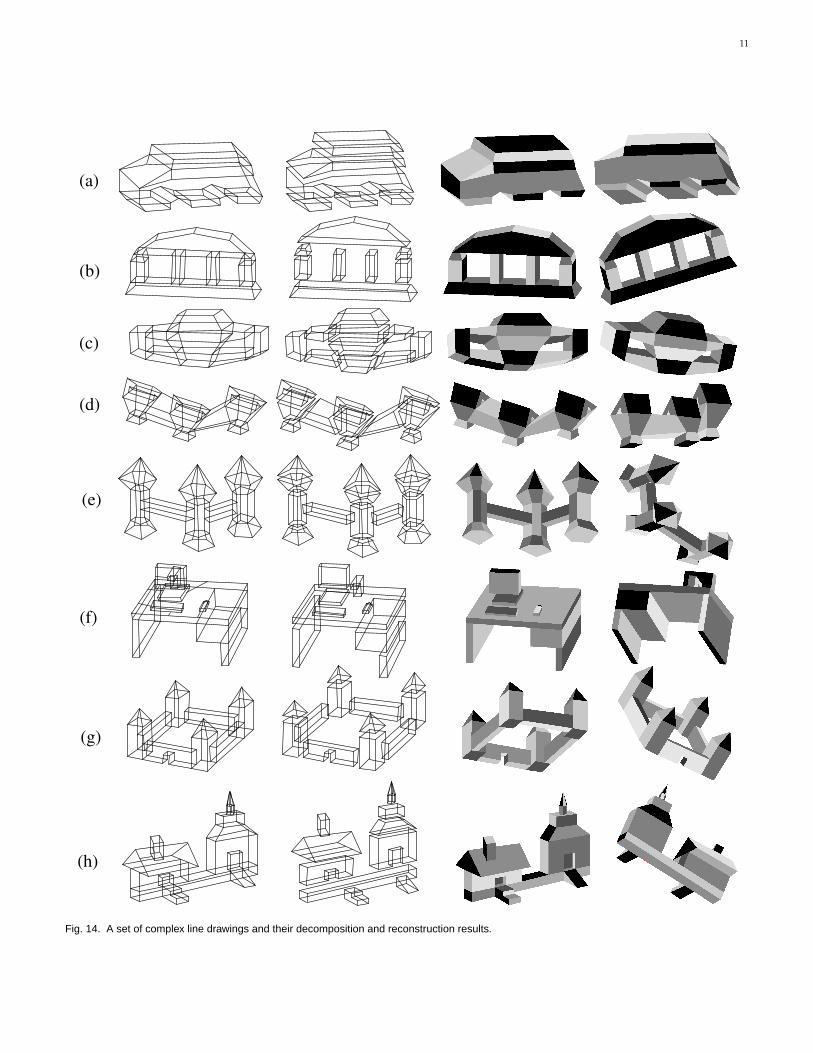
Fig. 14 shows a set of complex line drawings. Thereis only one decomposition from line drawing (a), (e), (f),or (g), but there are 8, 4, 8, and 4 decompositions fromline drawings (b), (c), (d), and (h), respectively. In Fig. 14,only one decomposition of each line drawing is given,together with the reconstructed 3D object displayed intwo views. From these results, we can see that our al-gorithm successfully decomposes the line drawings andgenerates desired 3D objects. It should be emphasizedthat the objects in Fig. 14 are more complex than theobjects given in the previous related papers, in terms ofthe numbers of real faces and internal faces.

The method in [9] can do 3D reconstruction of morecomplex objects than other previous methods. However,it is still unable to handle these complex line drawingsdue to too many real and internal faces in each object.From [9], we know that the dimension of the objectsearch space depends on the number of the internal facesof an object. A high dimensional search space renders thesearch for desired objects more difficult [9]. For example,from the line drawing (e) in Fig. 14, the algorithm in[9] generates an unexpected result as shown in Fig. 15.On the contrary, the 3D objects are easy to reconstructfrom the decomposed simple line drawings, and thecombination of them into one is also easy.

From the 3D reconstruction results in Fig. 14, we cansee that some are not perfect. For example, in the twosecond views of the results reconstructed from Figs. 14(g)and (h), the four walls of the castle are a little twisted,and the two ends of the base of the house are notof the same thickness. These imperfections come fromseveral factors: inaccurate sketches of line drawings, thesuperstrictness problem in this reconstruction problem[9], approximately optimal solutions obtained by theoptimization algorithm used in steps 3) and 5) in Algo-rithm 3, and the imperfect regularities used to constructthe objective function for 3D reconstruction [9], [18].

Common man-made objects such as those in Fig. 14are usually symmetric or regular with parallel or perpen-dicular faces. Our algorithm can also cope with irregularobjects. Fig. 16(a) shows the line drawing of such an

11

(a)

(b)

(c)

(d)

(e)

(f)

(g)

(h)

Fig. 14. A set of complex line drawings and their decomposition and reconstruction results.

12

(a) (b)

(c) (d) (e)

Fig. 16. (a) The line drawing of an irregular object. (b) Decompositionresult. (c) (d) (e) Reconstruction result displayed in three views.

TABLE 1Times (seconds) taken by searching for the internal faces (T1) andfine-tuning the complete objects (T2) for the line drawings in Fig.14.

T1

T2

a b c e f d g h

3

3

4

6

11

5

9

8

8

21

2

14

3

15

6

32

object. The decomposition and reconstruction results areshown in Figs. 16(b)–(e).

The computational time of Algorithm 3 varies withdifferent drawings, depending on their complexity. Themain computational cost comes from steps 1 and 5.Table 1 lists the times taken by these two steps for allthe line drawings in Fig. 14.

The next experiment is to show how the compu-tational time of Algorithm 1 varies for line drawingsof increasing size. In Fig. 17, seven objects O1−7 (linedrawings) are denoted by seven loops with Oi ⊂ Oi+1,1 ≤ i ≤ 6. They are shown this way to save space.The time used to find the internal faces of each object isplotted in Fig. 18. It can be seen that the time is not anexponential function of the size for these line drawings,indicating the usefulness of the proposed properties andthe efficiency of Algorithm 1 for internal face identifica-tion, even though the numbers of non-self-intersectingcycles (potential internal faces) of these line drawingsincrease exponentially. For O1−5, these numbers are 79,5310, 368465, 4479584, and 50108386, respectively.

There are two kinds of objects that Algorithm 1 cannotdecompose: objects without internal faces such as theone in Fig. 19(a) and objects whose internal faces are self-intersecting such as the one in Fig. 19(b) with the self-intersecting internal face (1, 2, 3, 4, 1). Here we explainmore about the second case. In this paper, we reconstruct3D planar-faced manifold objects from line drawings.It is reasonable to assume that internal faces are also

1 2

3

4

5

6

7

Fig. 17. Seven line drawings of increasing size denoted by seven loops.

1 0.138

4

2

6

8

12

10

14

16

20

18

22

Time (seconds)

2

1.445

3

3.642

4

7.830

5 6 7 Object

13.142

17.505

22.712

Fig. 18. The time used by Algorithm 1 to find the internal faces of theline drawings in Fig. 17.

planar and thus non-self-intersecting. If internal facesare allowed to be self-intersecting, two problems will beincurred: 1) Without the non-self-intersecting constraint,much more cycles in a complex line drawing can bethe candidates of internal faces and it is difficult todetermine the internal faces. 2) When a line drawingis decomposed, their internal faces become real faces inthe decomposed line drawings. These self-intersectingreal faces may cause previous 3D reconstruction meth-ods to fail because they are based on planar non-self-intersecting faces. In Figs. 19(c), (d), and (e), the internalfaces (1, 2, 3, 4, 1) are not self-intersecting and our algo-rithm can handle them easily. Dealing with the cases asin Figs. 19(a) and (b) is part of the future work.

13

1

2

3

4

1

2

3

4

1

2

3

4

1 2

3

4

(a) (b)

(c) (d) (e)

Fig. 19. (a) An object without internal faces. (b) An object with a self-intersecting internal face. (c) (d) (e) Objects with non-self-intersectinginternal faces.

6 CONCLUSION

In this paper, we have proposed a novel divide-and-conquer approach to complex 3D planar-faced manifoldreconstruction from single line drawings. Our strategyis to 1) identify the internal faces of an input linedrawing, 2) decompose the line drawing into simplerones along its internal faces, 3) reconstruct the 3D shapesfrom these simpler line drawings, and 4) merge theshapes into a complete object. The experiments showthat our approach can handle more complex objects thanprevious methods.

Future work includes 1) the improvement of the com-putational efficiency of the approach, 2) the beautifica-tion of the reconstructed objects, and 3) the extensionof the work to handle more general planar-faced objectsand objects with curved faces.

ACKNOWLEDGEMENTS

This work described in this paper was supported by agrant from the Research Grants Council of the HongKong SAR, China (Project No. CUHK 415408).

REFERENCES

[1] Y. Leclerc and M. Fischler, “An optimization-based approach tothe interpretation of single line drawings as 3D wire frames,” Int’lJournal of Computer Vision, vol. 9, no. 2, pp. 113–136, 1992.

[2] T. Marill, “Emulating the human interpretation of line-drawingsas three-dimensional objects,” Int’l Journal of Computer Vision,vol. 6, no. 2, pp. 147–161, 1991.

[3] K. Sugihara, “A necessary and sufficient condition for a pictureto represent a polyhedral scene,” IEEE Trans. Pattern Analysis andMachine Intelligence, vol. 6, no. 5, pp. 578–586, 1984.

[4] ——, Machine Interpretation of Line Drawings. MIT Press, 1986.[5] L. Ros and F. Thomas, “Overcoming superstrictness in line

drawing interpretation,” IEEE Trans. Pattern Analysis and MachineIntelligence, vol. 24, no. 4, pp. 456–466, 2002.

[6] J. Liu and Y. Lee, “A graph-based method for face identificationfrom a single 2D line drawing,” IEEE Trans. Pattern Analysis andMachine Intelligence, vol. 23, no. 10, pp. 1106–1119, 2001.

[7] J. Liu, Y. Lee, and W. K. Cham, “Identifying faces in a 2Dline drawing representing a manifold object,” IEEE Trans. PatternAnalysis and Machine Intelligence, vol. 24, no. 12, pp. 1579–1593,2002.

[8] J. Liu and X. Tang, “Evolutionary search for faces from linedrawings,” IEEE Trans. Pattern Analysis and Machine Intelligence,vol. 27, no. 6, pp. 861–872, 2005.

[9] J. Liu, L. Cao, Z. Li, and X. Tang, “Plane-based optimization for3D object reconstruction from single line drawings,” IEEE Trans.Pattern Analysis and Machine Intelligence, vol. 30, no. 2, pp. 315–327,2008.

[10] Y. Chen, J. Liu, and X. Tang, “A divide-and-conquer approachto 3D object reconstruction from line drawings,” IEEE Proc. Int’lConf. Computer Vision, 2007.

[11] K. Shoji, K. Kato, and F. Toyama, “3-D interpretation of single linedrawings based on entropy minimization principle,” IEEE Proc.Computer Vision and Pattern Recognition, vol. 2, pp. 90–95, 2001.

[12] M. Shpitalni and H. Lipson, “Identification of faces in a 2D linedrawing projection of a wireframe object,” IEEE Trans. PatternAnalysis and Machine Intelligence, vol. 18, no. 10, pp. 1000–1012,1996.

[13] S. C. Agarwal and J. W. N. Waggenspack, “Decomposition methodfor extracting face topologies from wireframe models,” Computer-Aided Design, vol. 24, no. 3, pp. 123–140, 1992.

[14] S. Bagali and J. Waggenspack, “A shortest path approach to wire-frame to solid model conversion,” Proc. 3rd Symp. Solid Modelingand Application, pp. 339–349, 1995.

[15] P. Company, M. Contero, J. Conesa, and A. Piquer, “Anoptimisation-based reconstruction engine for 3d modeling bysketching,” Computers & Graphics, vol. 28, pp. 955–979, 2004.

[16] P. Company, A. Piquer, M. Contero, and F. Naya, “A survey ongeometrical reconstruction as a core technology to sketch-basedmodeling,” Computer & Graphics, vol. 29, no. 6, pp. 892–904, 2005.

[17] P. Debevec, C. Yaylor, and J. Malik, “Modeling and renderingarchitecture from photograph: a hybrid geometry and image-based approach,” SIGGRAPH’96, pp. 11–20, 1996.

[18] H. Lipson and M. Shpitalni, “Optimization-based reconstructionof a 3D object from a single freehand line drawing,” Computer-Aided Design, vol. 28, no. 8, pp. 651–663, 1996.

[19] P. Min, J. Chen, and T. Funkhouser, “A 2D sketch interface fora 3D model search engine,” SIGGRAPH’02, Technical Sketches, p.138, 2002.

[20] A. Turner, D. Chapman, and A. Penn, “Sketching space,” Computerand Graphics, vol. 24, pp. 869–879, 2000.

[21] A. Piquer, R. R. Martin, and P. Company, “Using skewed mirrorsymmetry for optimisation-based 3D line-drawing recognition,”Proc. Fifth IAPR Int’l Workshop Graphics Recognition, pp. 182–193,2003.

[22] S. Ortiz, “3D searching starts to take shape,” Computer, vol. 37,no. 8, pp. 24–26, 2004.

[23] L. Cao, J. Liu, and X. Tang, “3D object retrieval using 2D linedrawing and graph based relevance feedback,” Proc. ACM Int’lConf. Multimedia, pp. 105–108, 2006.

[24] M. Clowes, “On seeing things,” Artificial Intelligence, vol. 2, pp.79–116, 1971.

[25] D. Huffman, “Impossible objects as nonsense sentences,” MachineIntelligence, vol. 6, pp. 295–323, 1971.

[26] K. Sugihara, “An algebraic approach to shape-from-image prob-lem,” Artificial Intelligence, vol. 23, pp. 59–95, 1984.

[27] M. C. Cooper, “Wireframe projections: Physical realisability ofcurved objects and unambiguous reconstruction of simple poly-hedra,” Int’l Journal of Computer Vision, vol. 64, no. 1, pp. 69–88,2005.

[28] ——, “Constraints between distant lines in the labelling of linedrawings of polyhedral scenes,” Int’l Journal of Computer Vision,vol. 73, no. 2, pp. 195–212, 2007.

[29] ——, “A rich discrete labeling scheme for line drawings of curvedobjects,” IEEE Trans. Pattern Analysis and Machine Intelligence,vol. 30, no. 4, pp. 741–745, 2008.

[30] H. Li, Q. Wang, L. Zhao, Y. Chen, and L. Huang, “nD object rep-resentation and detection from simple 2D line drawing,” LNCS,vol. 3519, pp. 363–382, 2005.

[31] P. A. C. Varley and R. R. Martin, “Estimating depth from linedrawings,” Proc. 7th ACM Symposium on Solid Modeling and Appli-cation, pp. 180–191, 2002.

14

[32] L. Cao, J. Liu, and X. Tang, “3D object reconstruction from asingle 2D line drawing without hidden lines,” IEEE Proc. Int’lConf. Computer Vision, vol. 1, pp. 272–277, 2005.

[33] ——, “What the back of the object looks like: 3D reconstructionfrom line drawings without hidden lines,” IEEE Trans. PatternAnalysis and Machine Intelligence, vol. 30, no. 3, pp. 507–517, 2008.

[34] I. Shimshoni and J. Ponce, “Recovering the shape of polyhedrausing line-drawing analysis and complex reflectance models,”Computer Vision and Image Processing, vol. 65, no. 2, pp. 296–310,1997.

[35] H. Shimodaira, “A shape-from-shading method of polyhedralobjects using prior information,” IEEE Trans. Pattern Analysis andMachine Intelligence, vol. 28, no. 4, pp. 612–624, 2006.

[36] P. A. C. Varley and R. R. Martin, “A system for constructingboundary representation solid models from a two-dimensionalsketch—topology of hidden parts,” Proc. First UK-Korea Workshopon Geometric Modeling and Computer Graphics, pp. 113–128, 2000.

[37] M. A. Armstrong, Basic Topology. Springer, 1983.[38] D. E. LaCourse, Handbook of Solid Modeling. New York: McGraw-

Hill, 1995.

Jianzhuang Liu received the B.E. degree from NanjingUniversity of Posts and Telecommunications, P. R. China,in 1983, the M.E. degree from Beijing University ofPosts and Telecommunications, P. R. China, in 1987,and the Ph.D. degree from The Chinese University ofHong Kong, Hong Kong, in 1997. From 1987 to 1994, hewas a faculty member in the Department of ElectronicEngineering, Xidian University, P. R. China. From Au-gust 1998 to August 2000, he was a research fellow atthe School of Mechanical and Production Engineering,Nanyang Technological University, Singapore. Then hewas a postdoctoral fellow in The Chinese Universityof Hong Kong for several years. He is now a researchassociate professor in the Department of InformationEngineering, The Chinese University of Hong Kong.His research interests include computer vision, imageprocessing, machine learning, and graphics.

Yu Chen received the B.E. degree from the Departmentof Electronics Engineering, Tsinghua University, P. R.China, in 2006, and the M.Phil. degree from the Depart-ment of Information Engineering, The Chinese Univer-sity of Hong Kong, Hong Kong, in 2008. He is currentlya Ph.D. candidate in the Department of Engineering,University of Cambridge, United Kingdom. His researchinterests include image processing and computer vision.

Xiaoou Tang received the B.S. degree from the Univer-sity of Science and Technology of China, Hefei, in 1990,and the M.S. degree from the University of Rochester,Rochester, NY, in 1991. He received the Ph.D. degreefrom the Massachusetts Institute of Technology, Cam-bridge, in 1996. He is a professor in the Departmentof Information Engineering, the Chinese University ofHong Kong. He worked as the group manager of theVisual Computing Group at the Microsoft Research Asiafrom 2005 to 2008. He received the Best Paper Awardat the IEEE Conference on Computer Vision and PatternRecognition (CVPR) 2009. Dr. Tang is a program chair ofthe IEEE International Conference on Computer Vision(ICCV) 2009 and an associate editor of IEEE Transactions

on Pattern Analysis and Machine Intelligence (PAMI)and International Journal of Computer Vision (IJCV). Heis a Fellow of IEEE. His research interests include com-puter vision, pattern recognition, and video processing.