DECOMPOSITIONAL SEMANTICS FOR EVENTS, PARTICIPANTS, …

DECOMPOSITIONAL SEMANTICS FOR EVENTS,

PARTICIPANTS, AND SCRIPTS IN TEXT

by

Rachel Rudinger

A dissertation submitted to The Johns Hopkins University in conformity with the

requirements for the degree of Doctor of Philosophy.

Baltimore, Maryland

October, 2019

c⃝ 2019 Rachel Rudinger

All rights reserved

Abstract

This thesis presents a sequence of practical and conceptual developments in

decompositional meaning representations for events, participants, and scripts in text

under the framework of Universal Decompositional Semantics (UDS) (White et al.,

2016a). Part I of the thesis focuses on the semantic representation of individual

events and their participants. Chapter 3 examines the feasibility of deriving semantic

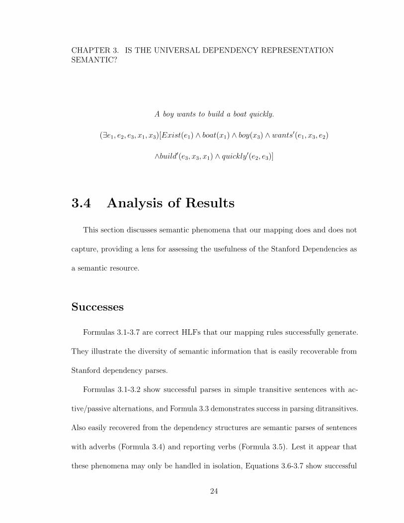
representations of events from dependency syntax; we demonstrate that predicate-

argument structure may be extracted from syntax, but other desirable semantic

attributes are not directly discernible. Accordingly, we present in Chapters 4 and 5

state of the art models for predicting these semantic attributes from text. Chapter

4 presents a model for predicting semantic proto-role labels (SPRL), attributes of

participants in events based on Dowty’s seminal theory of thematic proto-roles (Dowty,

1991). In Chapter 5 we present a model of event factuality prediction (EFP), the

task of determining whether an event mentioned in text happened (according to the

meaning of the text). Both chapters include extensive experiments on multi-task

learning for improving performance on each semantic prediction task. Taken together,

ii

ABSTRACT

Chapters 3, 4, and 5 represent the development of individual components of a UDS

parsing pipeline.

In Part II of the thesis, we shift to modeling sequences of events, or scripts

(Schank and Abelson, 1977). Chapter 7 presents a case study in script induction

using a collection of restaurant narratives from an online blog to learn the canonical

“Restaurant Script.” In Chapter 8, we introduce a simple discriminative neural

model for script induction based on narrative chains (Chambers and Jurafsky, 2008)

that outperforms prior methods. Because much existing work on narrative chains

employs semantically impoverished representations of events, Chapter 9 draws on the

contributions of Part I to learn narrative chains with semantically rich, decompositional

event representations. Finally, in Chapter 10, we observe that corpus based approaches

to script induction resemble the task of language modeling. We explore the broader

question of the relationship between language modeling and acquisition of common-

sense knowledge, and introduce an approach that combines language modeling and

light human supervision to construct datasets for common-sense inference.

Primary Reader and Advisor: Benjamin Van Durme

Secondary Reader: Kyle Rawlins, Aaron Steven White

iii

Acknowledgments

The long and, at times, arduous journey to earning a Ph.D. is one I could not

have successfully completed without the support and kindness of my many colleagues,

mentors, friends and family members. I am deeply indebted to them all, and hope to

have many opportunities in the years to come to pay these debts forward.

I am immensely grateful to my Ph.D. advisor, Ben Van Durme, from whom I have

learned not only how to conduct meaningful and high quality original research, but

also how to lead with compassion. Ben’s unwavering support and confidence in me over

many years have been invaluable. I am also thankful to my other committee members

Aaron White and Kyle Rawlins, both with whom it has been a great pleasure to

collaborate, and whose intellectual contributions have greatly influenced the direction

of this thesis.

It has been my great fortune to have many brilliant and kind colleagues while at

Johns Hopkins. Playing an important role in my graduate education have been the

many faculty (in addition to my committee) with whom I’ve had the opportunity to

work or interact frequently: Kevin Duh, Jason Eisner, Sanjeev Khudanpur, Raman

iv

ACKNOWLEDGMENTS

Arora, Mark Dredze, Matt Post, Philipp Koehn, David Yarowsky, Adam Lopez, Craig

Harman, Tom Lippincott, Jack Godfrey, and others. I have also been fortunate to

have many other excellent collaborators while at JHU: Tongfei Chen, Ryan Culkin,

Frank Ferraro, Xutai Ma, Chandler May, Arya McCarthy, Jason Naradowsky, Adam

Poliak, Pushpendre Rastogi, Dee Ann Reisinger, Keisuke Sakaguchi, Adam Teichert,

Tim Vieira, Sheng Zhang, Aparajita Haldar, Brian Leonard, Lisa Bauer, and Edward

Hu.

One of the most gratifying aspects of graduate school has been the incredible

network of peers at JHU. I cannot possibly name everyone, but, in addition to my

aforementioned collaborators, it has been a privilege getting to know and learn from:

Nick Andrews, Charley Beller, Adrian Benton, Andrew Blair-Stanek, Joshua Cape,

Annabelle Carrell, Eleanor Chodroff, Ryan Cotterell, Jeff Craley, Emory Davis, Ben

Diamond, Shuoyang Ding, Seth Ebner, Nathaniel Filardo, Matthew Francis-Landau,

Juri Ganitkevitch, Pegah Ghahremani, Mitchell Gordon, Matt Gormley, Katie Henry,

Nils Holzenberger, Ann Irvine, Jonathan Jones, Huda Khayrallah, Najoung Kim,

Chris Kirov, Rebecca Knowles, Gaurav Kumar, Keith Levin, Kunal Lillaney, Chu-

Cheng Lin, Celia Litovsky, Zachary Lubberts, Jane Lutken, Xutai Ma, Matthew

Maciejewski, Kelly Marchisio, Teodor Marinov, Rebecca Marvin, Chandler May, Tom

McCoy, Hongyuan Mei, Dan Mendat, Poorya Mianjy, Sebastian Mielke, Courtney

Napoles, Molly O’Brien, Princy Parsana, Michael Paul, Nanyun Peng, Guanghui Qin,

Desh Raj, Adithya Renduchintala, Darcey Riley, Naomi Saphra, Pamela Shapiro,

v

ACKNOWLEDGMENTS

Rachel Sherman, Ayushi Sinha, David Snyder, Sadhwi Srinivas, Elias Stengel-Eskin,

John Sylak-Glassman, Tim Vieira, Svitlana Volkova, Dingquan Wang, Felicity Wang,

Yiming Wang, Matthew Wiesner, Travis Wolfe, Zachary Wood-Doughty, Winston Wu,

Patrick Xia, Hainan Xu, Xuchen Yao, Xiaohui Zhang, Xuan Zhang, and many others.

During my Ph.D., I was fortunate to have opportunities to conduct research at

institutions outside JHU. Through the NSF PIRE program, I spent a semester as a

visiting Ph.D. student at the University of Saarland in Saarbrucken, Germany. I am

grateful to my hosts, Vera Demberg and Manfred Pinkal for their guidance early in my

Ph.D., and to the many others at Saarland University whom I had the opportunity

to work with or learn from: Fatemeh Torabi Asr, Matthew Crocker, Annemarie

Friedrich, Clayton Greenberg, Andrea Horbach, Evangelia Kiagia, Ashutosh Modi,

Alexis Palmer, Max Rabkin, Michaela Regneri, Asad Sayeed, Marc Schulder, Stefan

Thater, and many others. Through PIRE, I was also able to participate in the Fred

Jelinek Memorial Workshop at Charles University in Prague, so I am very thankful to

the workshop organizers both at Charles University and JHU. During my Ph.D., I

also had the opportunity to intern at the Allen Institute for Artificial Intelligence in

Seattle; many thanks to my host, Peter Clark, for his support.

I am also very grateful to the Center for Language and Speech Processing and the

Computer Science Department at Johns Hopkins for providing essential institutional

support. A very special thanks to Ruth Scally, Jennifer Linton, and Zack Burwell for

their help on countless occasions, and also to Carl Pupa for critical technical support.

vi

ACKNOWLEDGMENTS

I am also grateful to the Human Language Technologies Center of Excellence for the

computing and other resources they have generously allowed me over the years.

My decision to pursue a Ph.D. in Computer Science was deeply influenced by a

number of research mentors I worked with as an undergraduate who were incredibly

giving of their time and support. I am tremendously thankful to my undergraduate

research mentors at Yale, Dana Angluin, Bob Frank, and Brian Scassellati; to Lijun

Yin and Michael Lewis at Binghamton University for hosting me as an NSF REU

participant; and to my research mentors as an undergraduate participant in the JHU

CLSP summer workshop, Hal Daume III, Marine Carpuat, Alexander Fraser, and

Chris Quirk.

In the past year, many people have offered me invaluable professional advice. I

am grateful for the advice and encouragement I have received from: Ben Van Durme,

Aaron White, Kyle Rawlins, Mark Dredze, Chris Callison-Burch, Meg Mitchell, Peter

Clark, Martha Palmer, Nathan Schneider, Ed Hovy, Graham Neubig, Ellie Pavlick,

Sam Bowman, James Pustejovsky, Dan Jurafsky, Jason Eisner, Frank Ferraro, Cynthia

Matuszek, Jordan Boyd-Graber, Marine Carpuat, Hal Daume III, Naomi Feldman,

Doug Ouard, Philip Resnik, Noah Smith, Yejin Choi, Luke Zettlemoyer, Ben Zhao,

Lenhart Schubert, Dan Gildea, Dipanjan Das, and many others.

Pursuing a Ph.D. at JHU has brought me very close to a number of people through

the bond of shared challenges. I am incredibly lucky to have formed life-long friends

at JHU and in the greater Baltimore-DC area whose support and camaraderie during

vii

ACKNOWLEDGMENTS

the Ph.D. has meant the world to me: Keith Levin, Naomi Saphra, Rebecca Knowles,

Huda Khayrallah, Kate Fischl, Kira Riehm, Chandler May, Andrew Ruef, Alice

Jackson, Will Parker, Dana Craft-Parker, Casey Watts, Derek Caelin, and my dearest

friend and confidant, Mara Caelin.

I am deeply grateful for the support and love from my relatives and extended

family. Thank you to the Blazeks for providing a “home away from home” and being

a second family; your love and support mean so much to me. Thank you to Mark and

Char, the Kuhns, the Taenzers, the Glasers, and all of my extended family in Arizona;

I’m fortunate to have such loving family all across the country.

I am incredibly grateful to my loving grandmother, Florence, who has always been

an important part of my life, and from whom I have inherited a love of science, travel,

and good food. I am also thankful for the memories of my other grandparents, Leo,

Frances, George, and Ellen. Each of these individuals were remarkable in their own

way and their memories are an inspiration to me. Ellen, a Jewish medical student in

Nazi Germany, escaped to the U.S. in 1937 where she finished her training and went

on to run her own medical practice in Buffalo, New York. Though she died before

I was born, her story has given me the courage to believe that I could succeed as a

woman in the field of Computer Science, and has given me the perspective to not lose

hope or humor in politically troubled times.

Finally, I wish to thank my immediate family. Mom, Dad, and Kenny: it is an

immense privilege to have family members who are attuned to the unique challenges

viii

ACKNOWLEDGMENTS

of a Ph.D. Your understanding, care, and support mean everything to me, and I could

not have done this without you. I am blessed with a family that I not only love but

like. Thank you for everything.

The work presented in this thesis was supported by a NSF Graduate Research

Fellowship (Grant No. DGE-1232825), NSF PIRE (0530118), the Paul Allen Institute

for Artificial Intelligence, the JHU HLTCOE, DARPA AIDA, DARPA LORELEI,

and DARPA DEFT. The views and conclusions contained in this publication are

those of the author and should not be interpreted as representing official policies or

endorsements of DARPA, NSF, or the U.S. Government.

ix

Dedication

To my family.

x

Contents

Abstract ii

Acknowledgments iv

List of Tables xvi

List of Figures xix

1 Introduction 1

I Events 5

2 Background and Overview, Part I 6

3 Is the Universal Dependency Representation Semantic? 14

3.1 Introduction . . . . . . . . . . . . . . . . . . . . . . . . . . . . . . . . 16

3.2 Background . . . . . . . . . . . . . . . . . . . . . . . . . . . . . . . . 17

3.3 Mapping to HLF . . . . . . . . . . . . . . . . . . . . . . . . . . . . . 19

xi

CONTENTS

3.4 Analysis of Results . . . . . . . . . . . . . . . . . . . . . . . . . . . . 24

3.5 Conclusion . . . . . . . . . . . . . . . . . . . . . . . . . . . . . . . . . 28

4 Neural-Davidsonian Semantic Proto-Role Labeling 30

4.1 Introduction . . . . . . . . . . . . . . . . . . . . . . . . . . . . . . . . 31

4.2 Background . . . . . . . . . . . . . . . . . . . . . . . . . . . . . . . . 33

4.3 “Neural-Davidsonian” Model . . . . . . . . . . . . . . . . . . . . . . . 35

4.4 Data . . . . . . . . . . . . . . . . . . . . . . . . . . . . . . . . . . . . 39

4.5 Experiments . . . . . . . . . . . . . . . . . . . . . . . . . . . . . . . . 42

4.6 Mult-Task Investigation . . . . . . . . . . . . . . . . . . . . . . . . . 46

4.6.1 Auxiliary Tasks . . . . . . . . . . . . . . . . . . . . . . . . . . 49

4.6.2 Results . . . . . . . . . . . . . . . . . . . . . . . . . . . . . . . 52

4.7 Conclusion . . . . . . . . . . . . . . . . . . . . . . . . . . . . . . . . . 59

5 Event Factuality Prediction 60

5.1 Introduction . . . . . . . . . . . . . . . . . . . . . . . . . . . . . . . . 61

5.2 Background . . . . . . . . . . . . . . . . . . . . . . . . . . . . . . . . 63

5.2.1 Linguistic description . . . . . . . . . . . . . . . . . . . . . . . 63

5.2.2 Event factuality datasets . . . . . . . . . . . . . . . . . . . . . 66

5.2.3 Event factuality systems . . . . . . . . . . . . . . . . . . . . . 68

5.3 Data collection . . . . . . . . . . . . . . . . . . . . . . . . . . . . . . 69

5.4 Models . . . . . . . . . . . . . . . . . . . . . . . . . . . . . . . . . . . 72

xii

CONTENTS

5.4.1 Stacked bidirectional linear LSTM . . . . . . . . . . . . . . . . 73

5.4.2 Stacked bidirectional tree LSTM . . . . . . . . . . . . . . . . 73

5.4.3 Regression model . . . . . . . . . . . . . . . . . . . . . . . . . 76

5.5 Experiments . . . . . . . . . . . . . . . . . . . . . . . . . . . . . . . . 77

5.6 Results . . . . . . . . . . . . . . . . . . . . . . . . . . . . . . . . . . . 84

5.7 Analysis . . . . . . . . . . . . . . . . . . . . . . . . . . . . . . . . . . 87

5.8 Conclusion . . . . . . . . . . . . . . . . . . . . . . . . . . . . . . . . . 90

II Scripts 92

6 Background and Overview, Part II 93

6.1 Related Work on Script Induction . . . . . . . . . . . . . . . . . . . . 95

7 The Restaurant Script 100

7.1 Related Work . . . . . . . . . . . . . . . . . . . . . . . . . . . . . . . 101

7.1.1 Narrative Chains . . . . . . . . . . . . . . . . . . . . . . . . . 102

7.2 Models . . . . . . . . . . . . . . . . . . . . . . . . . . . . . . . . . . . 104

7.2.1 Count-based Methods . . . . . . . . . . . . . . . . . . . . . . 105

7.3 Dataset: Dinners From Hell . . . . . . . . . . . . . . . . . . . . . . . 108

7.3.1 Annotation . . . . . . . . . . . . . . . . . . . . . . . . . . . . 109

7.4 Evaluation . . . . . . . . . . . . . . . . . . . . . . . . . . . . . . . . . 111

7.4.1 Narrative Cloze . . . . . . . . . . . . . . . . . . . . . . . . . . 111

xiii

CONTENTS

7.4.2 Qualitative Example . . . . . . . . . . . . . . . . . . . . . . . 114

7.5 Conclusion . . . . . . . . . . . . . . . . . . . . . . . . . . . . . . . . . 115

8 A Neural Sequence Model for Script Induction 116

8.1 Data Preparation . . . . . . . . . . . . . . . . . . . . . . . . . . . . . 117

8.2 Models . . . . . . . . . . . . . . . . . . . . . . . . . . . . . . . . . . . 118

8.3 Experimental Results . . . . . . . . . . . . . . . . . . . . . . . . . . . 122

8.4 Conclusion . . . . . . . . . . . . . . . . . . . . . . . . . . . . . . . . . 123

9 Decompositional Script Induction 125

9.1 Data Preparation . . . . . . . . . . . . . . . . . . . . . . . . . . . . . 126

9.2 Decompositional Narrative Chains . . . . . . . . . . . . . . . . . . . . 127

9.3 Extraction Pipeline . . . . . . . . . . . . . . . . . . . . . . . . . . . . 128

9.4 Narrative Cloze Construction . . . . . . . . . . . . . . . . . . . . . . 131

9.5 Model . . . . . . . . . . . . . . . . . . . . . . . . . . . . . . . . . . . 131

9.6 Experiments and Discussion . . . . . . . . . . . . . . . . . . . . . . . 134

9.7 Discussion . . . . . . . . . . . . . . . . . . . . . . . . . . . . . . . . . 138

9.8 Conclusion . . . . . . . . . . . . . . . . . . . . . . . . . . . . . . . . . 139

10 Common Sense and Language Modeling 141

10.1 Common-sense Inference . . . . . . . . . . . . . . . . . . . . . . . . . 143

10.2 A Generation Strategy for Common-sense Inference . . . . . . . . . . 145

10.2.1 Inference Generation via Language Models . . . . . . . . . . . 145

xiv

CONTENTS

10.2.2 Ordinal Likelihood Annotation . . . . . . . . . . . . . . . . . 149

10.3 Discussion . . . . . . . . . . . . . . . . . . . . . . . . . . . . . . . . . 150

11 Conclusion 153

11.1 Contributions . . . . . . . . . . . . . . . . . . . . . . . . . . . . . . . 153

11.2 Future Work . . . . . . . . . . . . . . . . . . . . . . . . . . . . . . . . 155

Vita 199

xv

List of Tables

2.1 A summary comparison of different semantic representations of textfor certain salient criteria. Note that the listed criteria (rows) are non-exhaustive and not formally defined, such that their implementationmay differ across schemas. . . . . . . . . . . . . . . . . . . . . . . . . 12

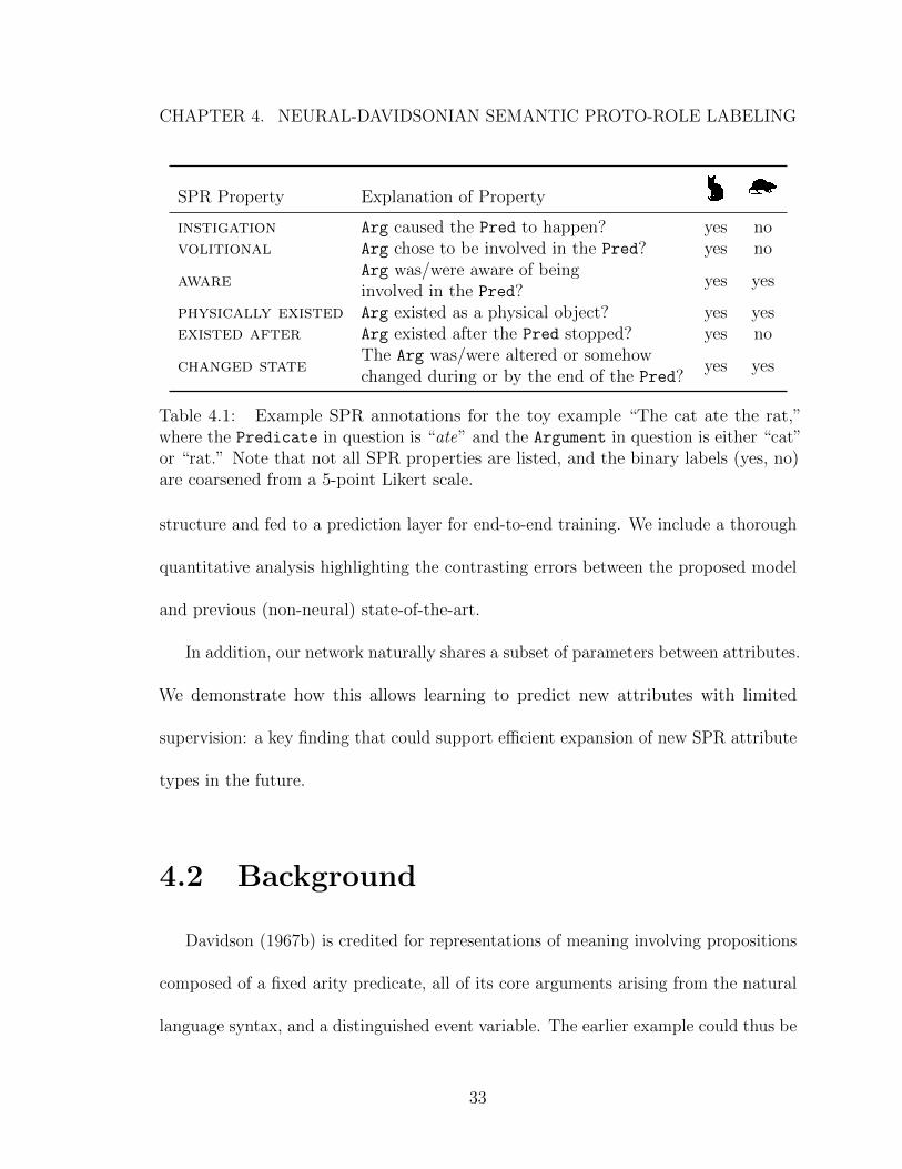
4.1 Example SPR annotations for the toy example “The cat ate the rat,”where the Predicate in question is “ate” and the Argument in questionis either “cat” or “rat.” Note that not all SPR properties are listed,and the binary labels (yes, no) are coarsened from a 5-point Likert scale. 33

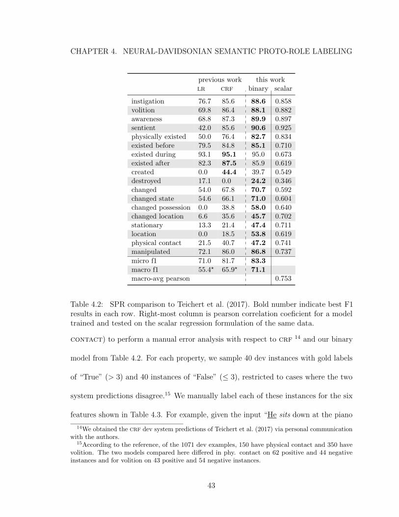
4.2 SPR comparison to Teichert et al. (2017). Bold number indicate best F1results in each row. Right-most column is pearson correlation coeficientfor a model trained and tested on the scalar regression formulation ofthe same data. . . . . . . . . . . . . . . . . . . . . . . . . . . . . . . 43

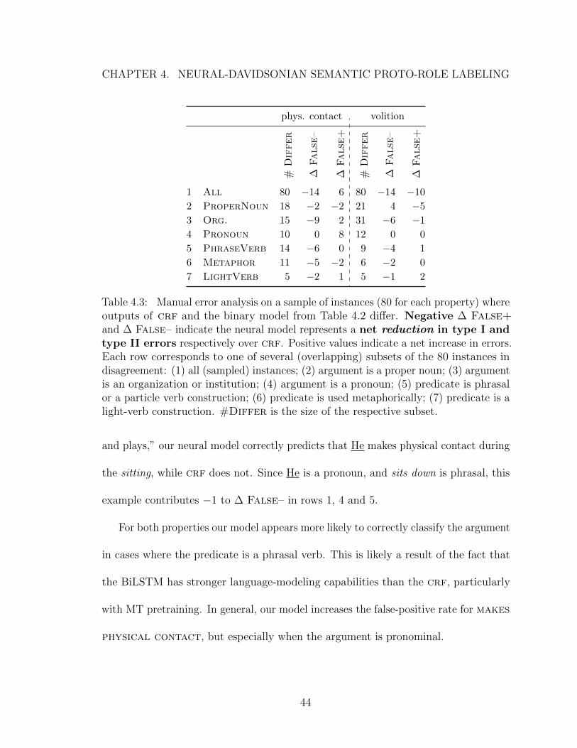
4.3 Manual error analysis on a sample of instances (80 for each property)where outputs of crf and the binary model from Table 4.2 differ. Neg-ative ∆ False+ and ∆ False– indicate the neural model represents anet reduction in type I and type II errors respectively over crf.Positive values indicate a net increase in errors. Each row corresponds toone of several (overlapping) subsets of the 80 instances in disagreement:(1) all (sampled) instances; (2) argument is a proper noun; (3) argu-ment is an organization or institution; (4) argument is a pronoun; (5)predicate is phrasal or a particle verb construction; (6) predicate is usedmetaphorically; (7) predicate is a light-verb construction. #Differ isthe size of the respective subset. . . . . . . . . . . . . . . . . . . . . 44

4.4 Name and short description of each experimental condition reported;numbering corresponds to experiment numbers reported in Section4.6.2. mt: indicates pretraining with machine translation; pb: indicatespretraining with PropBank SRL. . . . . . . . . . . . . . . . . . . . . 47

xvi

LIST OF TABLES

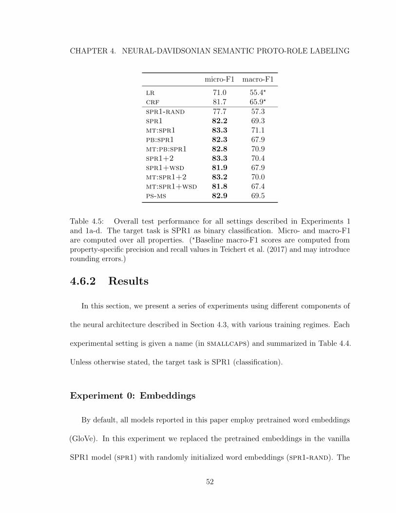
4.5 Overall test performance for all settings described in Experiments 1and 1a-d. The target task is SPR1 as binary classification. Micro-and macro-F1 are computed over all properties. (⋆Baseline macro-F1scores are computed from property-specific precision and recall valuesin Teichert et al. (2017) and may introduce rounding errors.) . . . . . 52

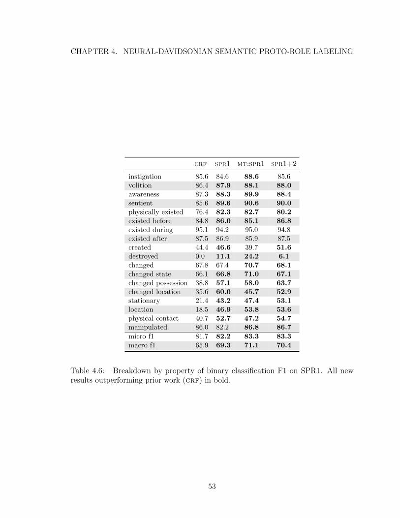
4.6 Breakdown by property of binary classification F1 on SPR1. All newresults outperforming prior work (crf) in bold. . . . . . . . . . . . . 53

4.7 SPR1 and SPR2 as scalar prediction tasks. Pearson correlation betweenpredicted and gold values. . . . . . . . . . . . . . . . . . . . . . . . . 56

4.8 SPR1 and SPR2 as scalar prediction tasks. The overall performance foreach experimental setting is reported as the average Pearson correlationover all properties. Highest SPR1 and SPR2 results are in bold. . . . 57

5.1 Number of annotated predicates. . . . . . . . . . . . . . . . . . . . . 685.2 Implication signature features from Nairn, Condoravdi, and Karttunen

(2006). As an example, a signature of −|+ indicates negative implicationunder positive polarity (left side) and positive implication under negativepolarity (right side); ◦ indicates neither positive nor negative implication. 79

5.3 Implicative (bold) and non-implicative (not bold) verbs from Karttunen(1971a) are nearly separable by our tense agreement scores, replicatingthe results of PC. . . . . . . . . . . . . . . . . . . . . . . . . . . . . . 80

5.4 All temporal phrases used to instantiate the $TIME variable for miningimplicative verb features. . . . . . . . . . . . . . . . . . . . . . . . . . 81

5.5 All 2-layer systems, and 1-layer systems if best in column. State-of-the-art in bold; † is best in column (with row shaded in purple).Key: L=linear, T=tree, H=hybrid, (1,2)=# layers, S=single-taskspecific, G=single-task general, +lexfeats=with all lexical features,MultiSimp=multi-task simple, MultiBal=multi-task balanced, MultiFoc=multi-task focused, w/UDS-IH2=trained on all data incl. UDS-IH2. All-3.0is the constant baseline. . . . . . . . . . . . . . . . . . . . . . . . . . 85

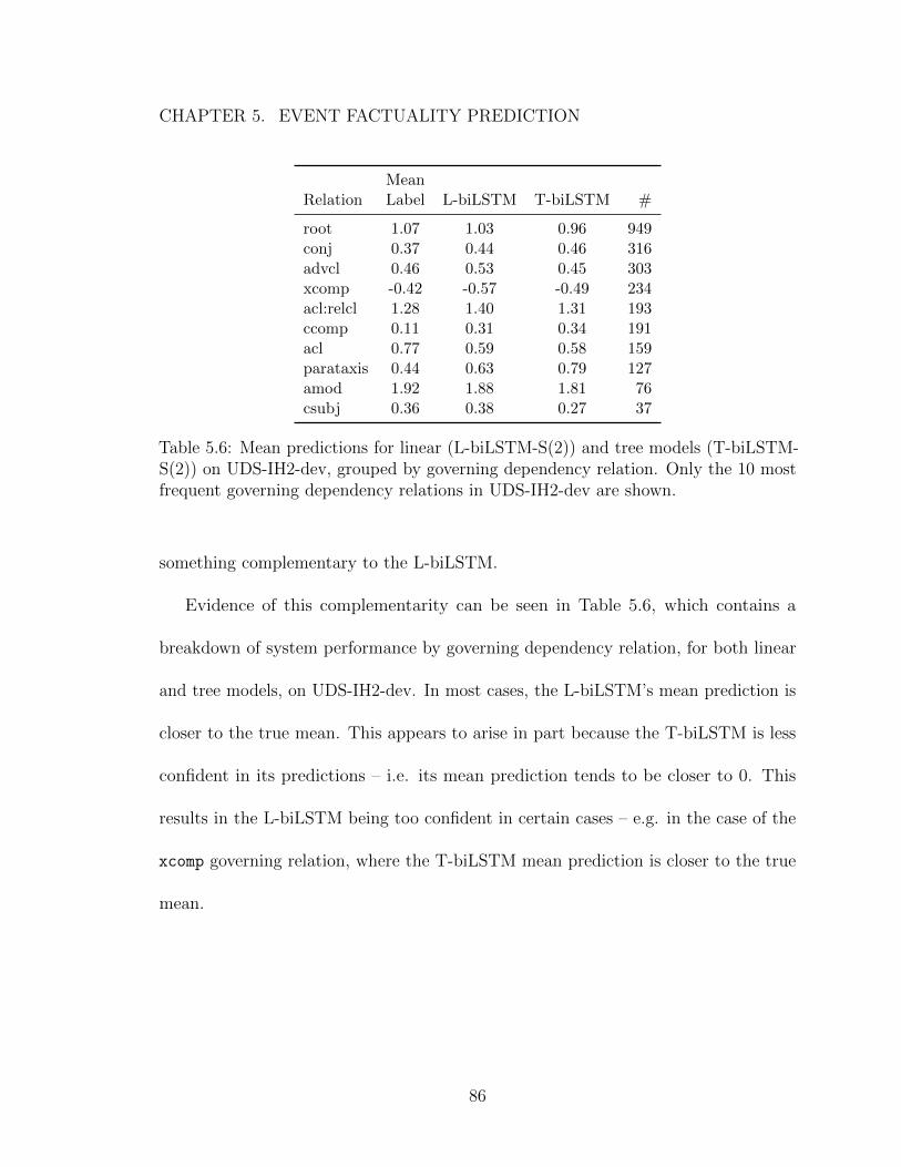
5.6 Mean predictions for linear (L-biLSTM-S(2)) and tree models (T-biLSTM-S(2)) on UDS-IH2-dev, grouped by governing dependencyrelation. Only the 10 most frequent governing dependency relations inUDS-IH2-dev are shown. . . . . . . . . . . . . . . . . . . . . . . . . . 86

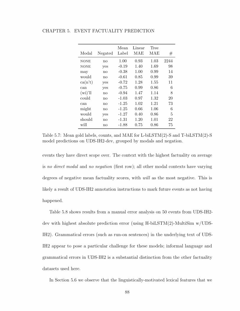
5.7 Mean gold labels, counts, and MAE for L-biLSTM(2)-S and T-biLSTM(2)-S model predictions on UDS-IH2-dev, grouped by modals and negation. 88

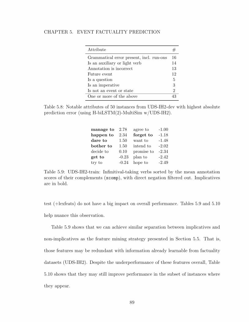
5.8 Notable attributes of 50 instances from UDS-IH2-dev with highestabsolute prediction error (using H-biLSTM(2)-MultiSim w/UDS-IH2). 89

5.9 UDS-IH2-train: Infinitival-taking verbs sorted by the mean annotationscores of their complements (xcomp), with direct negation filtered out.Implicatives are in bold. . . . . . . . . . . . . . . . . . . . . . . . . . 89

xvii

LIST OF TABLES

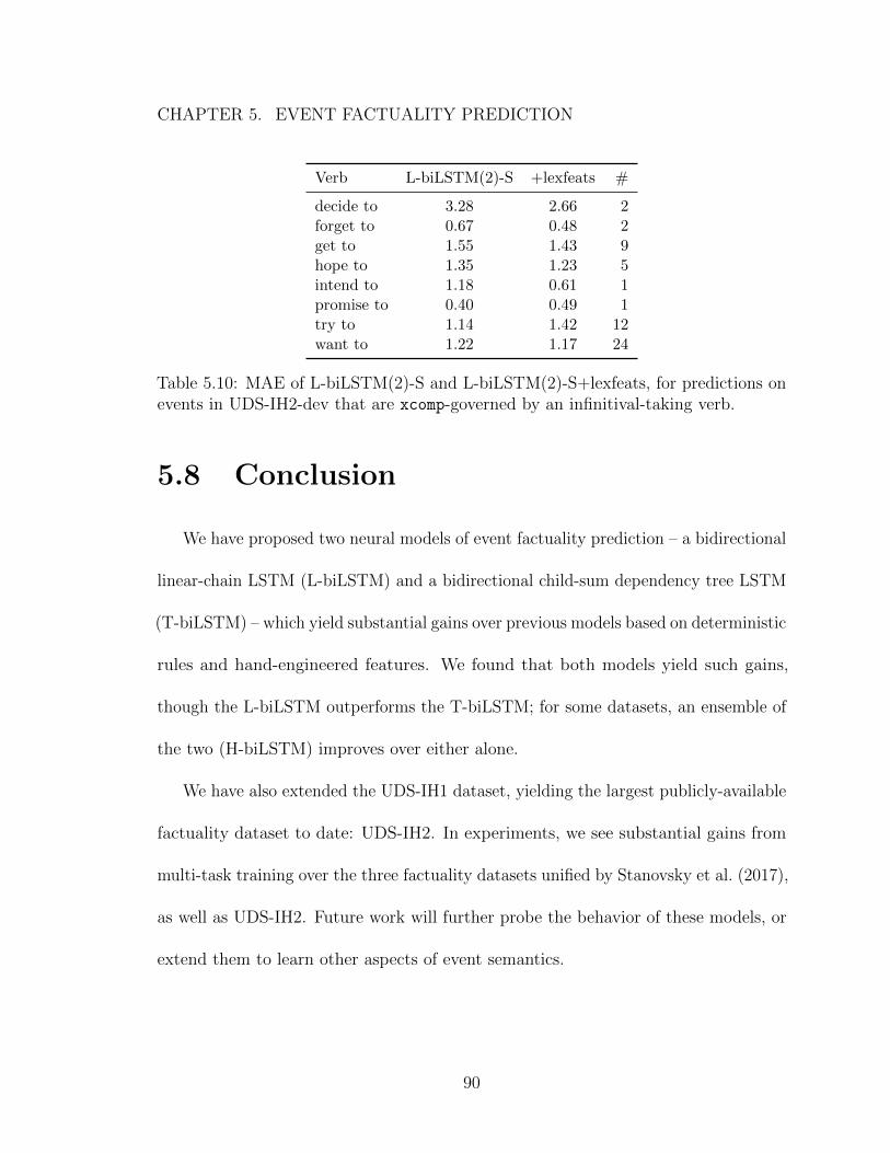
5.10 MAE of L-biLSTM(2)-S and L-biLSTM(2)-S+lexfeats, for predictionson events in UDS-IH2-dev that are xcomp-governed by an infinitival-taking verb. . . . . . . . . . . . . . . . . . . . . . . . . . . . . . . . . 90

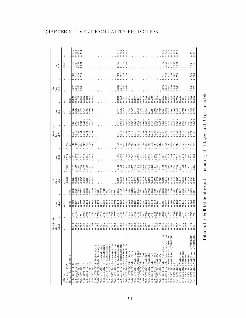
5.11 Full table of results, including all 1-layer and 2-layer models. . . . . . 91

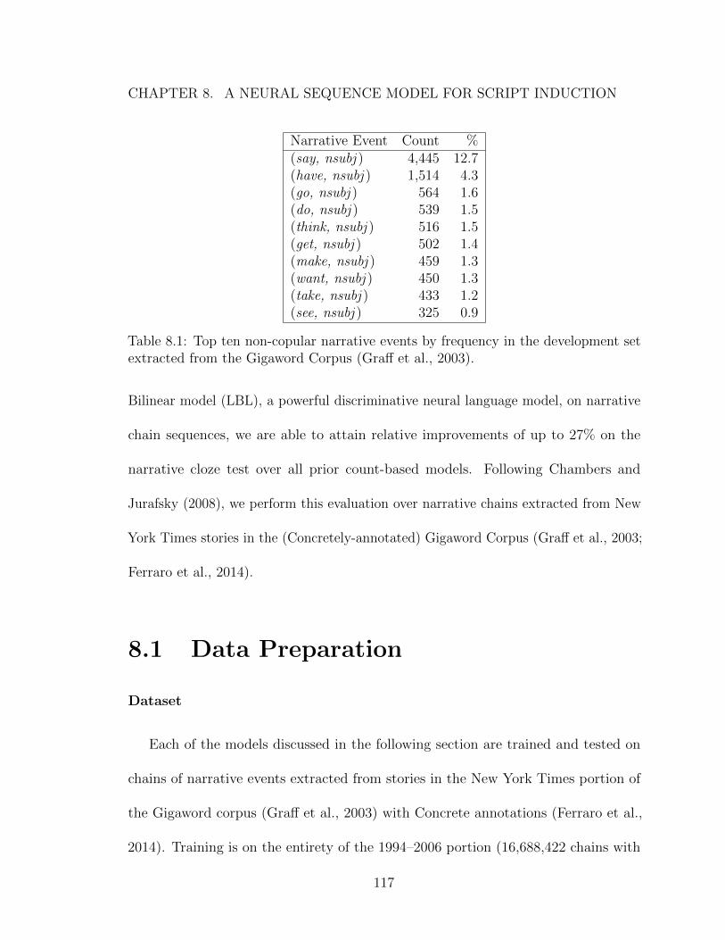
8.1 Top ten non-copular narrative events by frequency in the developmentset extracted from the Gigaword Corpus (Graff et al., 2003). . . . . . 117

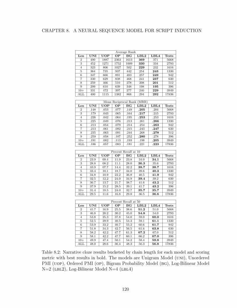
8.2 Narrative cloze results bucketed by chain length for each model andscoring metric with best results in bold. The models are Unigram Model(uni), Unordered PMI (uop), Ordered PMI (op), Bigram ProbabilityModel (bg), Log-Bilinear Model N=2 (lbl2), Log-Bilinear Model N=4(lbl4) . . . . . . . . . . . . . . . . . . . . . . . . . . . . . . . . . . . 120

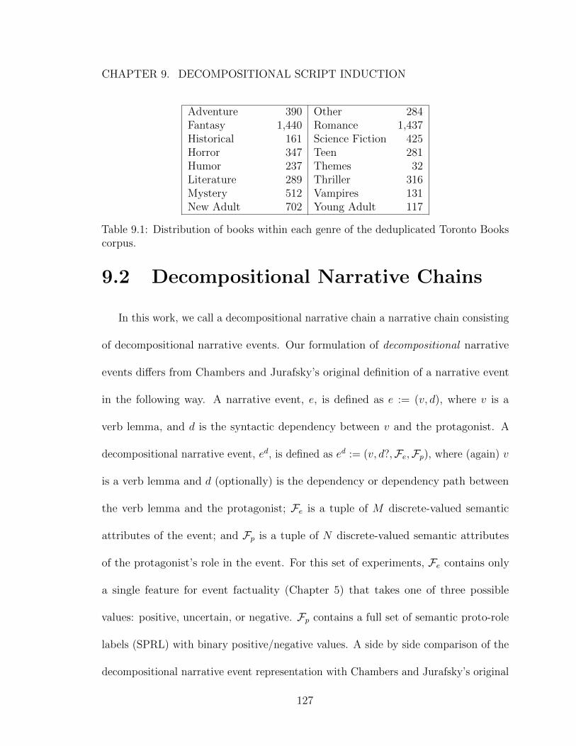
9.1 Distribution of books within each genre of the deduplicated TorontoBooks corpus. . . . . . . . . . . . . . . . . . . . . . . . . . . . . . . . 127

9.2 A comparison of the original syntactic narrative event representation(NE) of Chambers et al. (2007) with the proposed decompositionalnarrative event representation (DNE). These two examples are derivedfrom the example sentence “The cat ate the rat.” (in which we supposethe rat was the protagonist of a longer story). . . . . . . . . . . . . . 128

9.3 Names and descriptions of each experimental setting. For example,s2d is the “syntactic-to-decompositional” setting, in which the miss-ing (cloze) decompositional narrative event must be decoded given asurrounding sequence of syntactic narrative events. . . . . . . . . . . 135

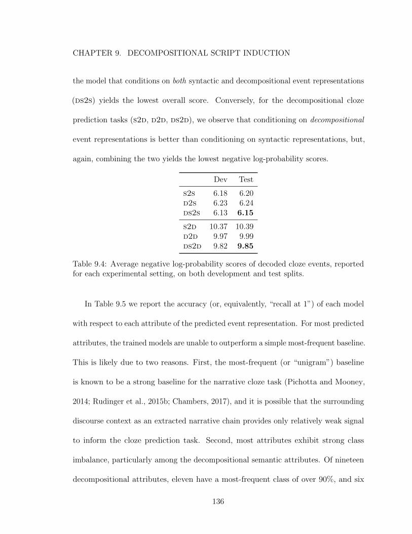
9.4 Average negative log-probability scores of decoded cloze events, reportedfor each experimental setting, on both development and test splits. . 136

9.5 Test accuracy (percentage) for both syntactic and decompositionalcloze tasks, broken down by each attribute of the narrative eventrepresentation. Comparison with a most-frequent baseline is included. 137

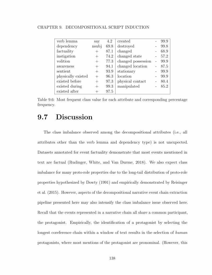
9.6 Most frequent class value for each attribute and corresponding percent-age frequency. . . . . . . . . . . . . . . . . . . . . . . . . . . . . . . . 138

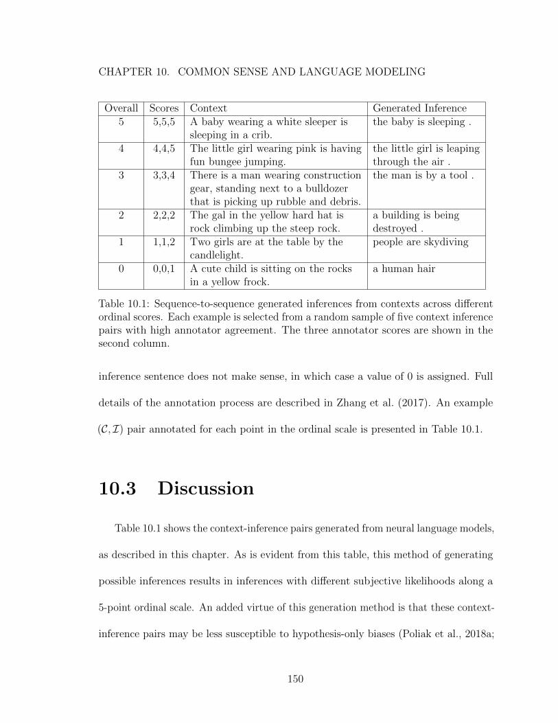
10.1 Sequence-to-sequence generated inferences from contexts across differentordinal scores. Each example is selected from a random sample of fivecontext inference pairs with high annotator agreement. The threeannotator scores are shown in the second column. . . . . . . . . . . . 150

xviii

List of Figures

1.1 An example of an award-winning chatbot, “Mitsuku,” failing to respondappropriately to a human user. (Inappropriate responses in red italics.)https://www.pandorabots.com/mitsuku/ . . . . . . . . . . . . . . . 2

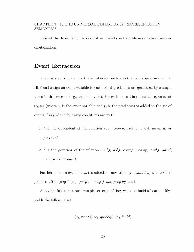
3.1 Stanford dependency parse of “A boy wants to build a boat quickly.” 18

4.1 BiLSTM sentence encoder with SPR decoder. Semantic proto-rolelabeling is with respect to a specific predicate and argument within asentence, so the decoder receives the two corresponding hidden states. 32

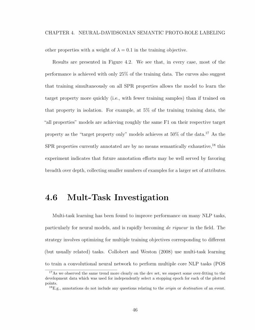
4.2 Effect of using only a fraction of the training data for a property whileeither ignoring or co-training with the full training data for the otherSPR1 properties. Measurements at 1%, 5%, 10%, 25%, 50%, and 100%. 45

5.1 Event factuality (⊕=factual) and inside v. outside context for leave inthe dependency tree. . . . . . . . . . . . . . . . . . . . . . . . . . . . 62

5.2 Relative frequency of factuality ratings in training and development sets. 71

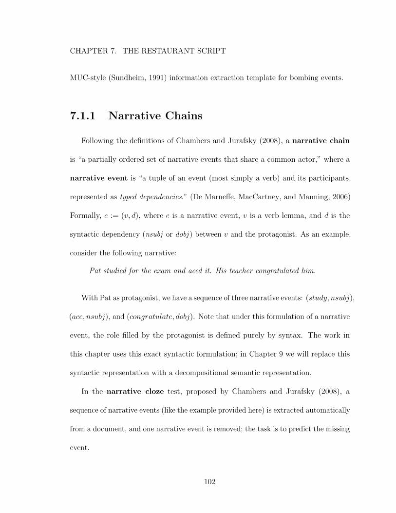
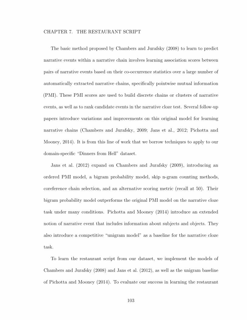
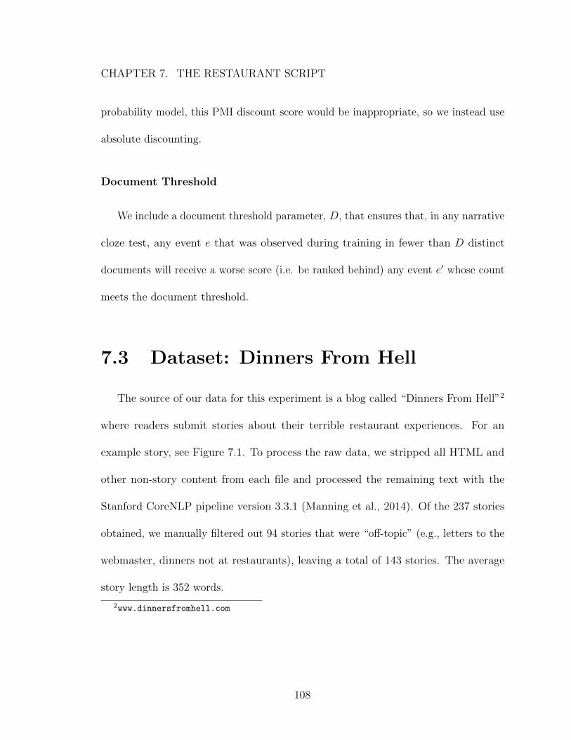
7.1 Example story from Dinners from Hell corpus. Bold words indicateevents in the “we” coreference chain (the longest chain). Boxed words(blue) indicate best narrative chain of length three (see Section 5.2);underlined words (orange) are corresponding subjects and bracketedwords (green) are corresponding objects. . . . . . . . . . . . . . . . . 109

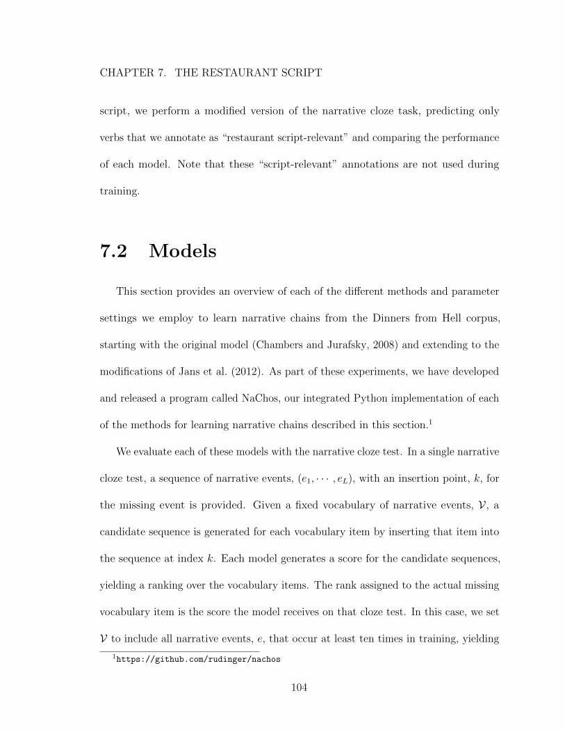
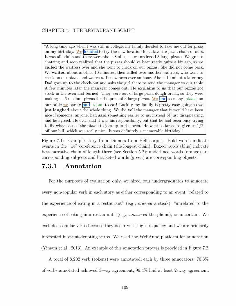
7.2 WebAnno interface for labeling non-copular verbs as denoting of eventsrelevant to the restaurant script (+ + +) or not relevant (−−−). . . 110

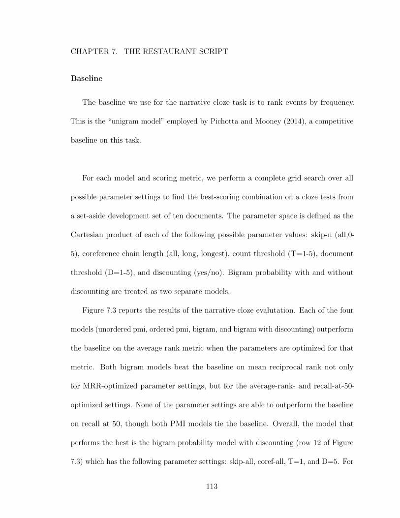
7.3 Narrative cloze evaluation. Shaded blue cells indicate which scoringmetric that row’s parameter settings have been optimized to. Boldnumbers indicate a result that beats the baseline. Row 12 representesthe best model performance overall. . . . . . . . . . . . . . . . . . . . 111

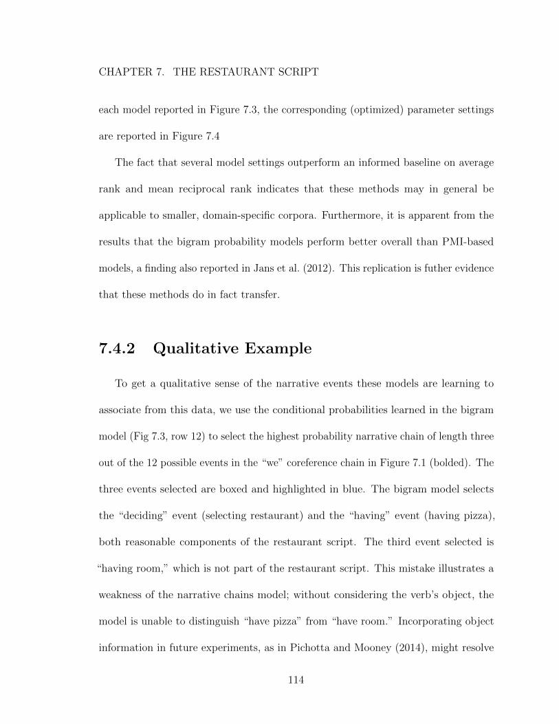
7.4 Parameter settings corresponding to each model in Fig 7.3. . . . . . . 112

xix

https://www.pandorabots.com/mitsuku/

LIST OF FIGURES

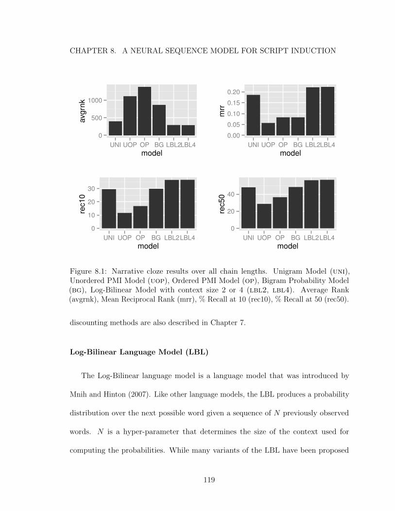
8.1 Narrative cloze results over all chain lengths. Unigram Model (uni),Unordered PMI Model (uop), Ordered PMI Model (op), Bigram Prob-ability Model (bg), Log-Bilinear Model with context size 2 or 4 (lbl2,lbl4). Average Rank (avgrnk), Mean Reciprocal Rank (mrr), % Recallat 10 (rec10), % Recall at 50 (rec50). . . . . . . . . . . . . . . . . . . 119

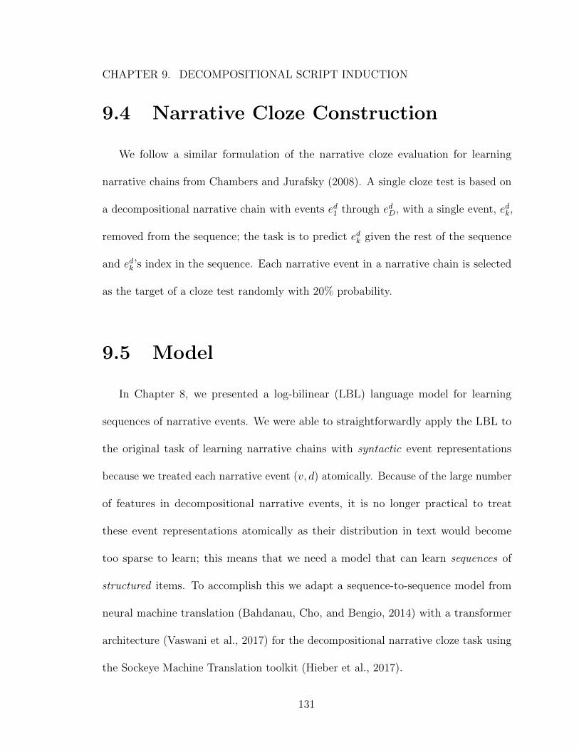
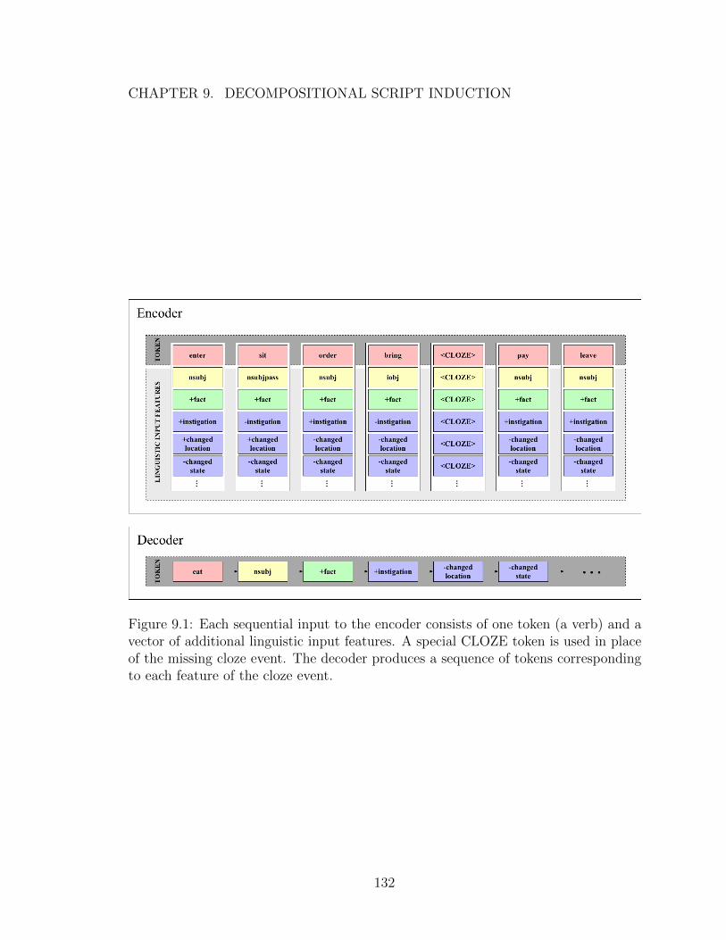
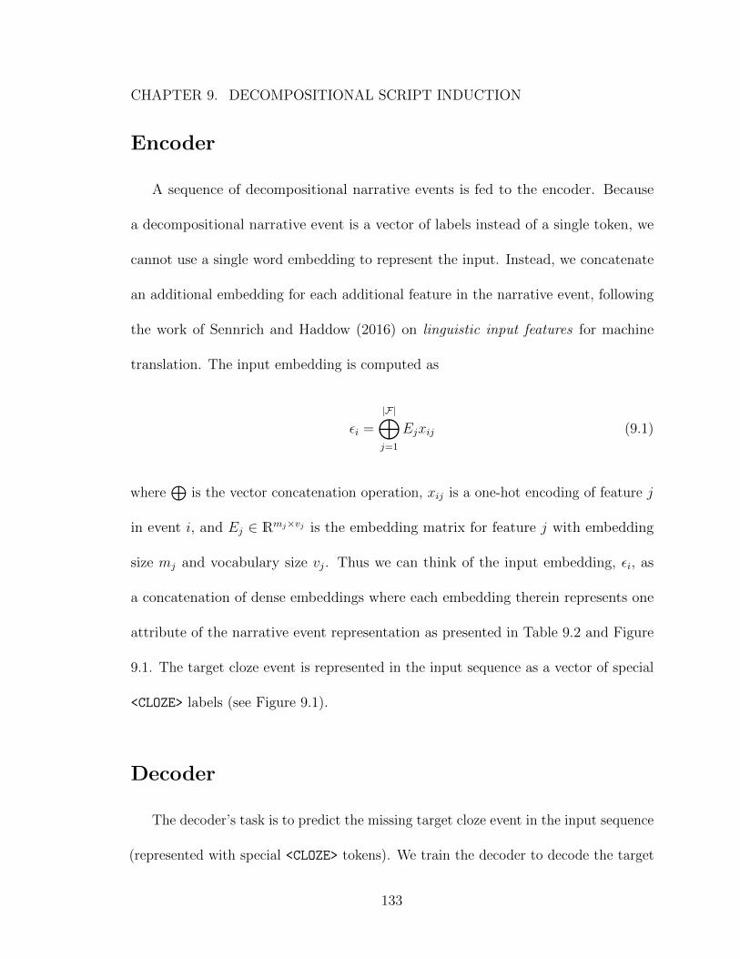
9.1 Each sequential input to the encoder consists of one token (a verb) anda vector of additional linguistic input features. A special CLOZE tokenis used in place of the missing cloze event. The decoder produces asequence of tokens corresponding to each feature of the cloze event. . 132

10.1 Examples of sequence-to-sequence inference generation from single-wordand full-sentence inputs. . . . . . . . . . . . . . . . . . . . . . . . . . 147

xx

Chapter 1

Introduction

It is the overarching goal of researchers in natural language processing (NLP) and

artificial intelligence to develop systems that have the capability to understand and

communicate fluently in human languages. The potential applications are myriad:

autonomous vehicle interfaces, question-answering systems, summarization of medical

health records, interactive game playing and story generation, educational language

instruction tools, among many others. Despite rapid progress in NLP in recent years

due to the statistical and neural “revolutions” within the field, existing NLP systems

are still error-prone because they lack a full-fledged understanding of the meaning

present in text, often relying instead on shallow pattern-matching statistics. We can

observe these limitations in the seemingly simple mistakes that these systems make,

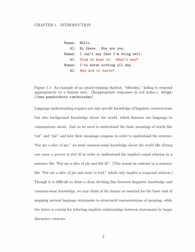
as shown in Figure 1.1.

Of course, developing robust models of language meaning is a difficult problem.

1

CHAPTER 1. INTRODUCTION

Human: Hello.

AI: Hi there. How are you.

Human: I can’t say that I’m doing well.

AI: Glad to hear it. What’s new?

Human: I’ve eaten nothing all day.

AI: How did it taste?

Figure 1.1: An example of an award-winning chatbot, “Mitsuku,” failing to respondappropriately to a human user. (Inappropriate responses in red italics.) https:

//www.pandorabots.com/mitsuku/

Language understanding requires not only specific knowledge of linguistic constructions,

but also background knowledge about the world, which humans use language to

communicate about. Just as we need to understand the basic meanings of words like

“eat” and “pie” and how their meanings compose in order to understand the sentence

“Pat ate a slice of pie,” we need common-sense knowledge about the world like Eating

can cause a person to feel ill in order to understand the implied causal relation in a

sentence like “Pat ate a slice of pie and felt ill.” (This stands in contrast to a sentence

like “Pat ate a slice of pie and went to bed,” which only implies a temporal relation.)

Though it is difficult to draw a clean dividing line between linguistic knowledge and

common-sense knowledge, we may think of the former as essential for the basic task of

mapping natural language statements to structured representations of meaning, while

the latter is crucial for inferring implicit relationships between statements in larger

discursive contexts.

2




It is in this setting, then, that this thesis will present a series of computational

models that seek to address key components of language meaning and understanding in

English. Parts I and II of this thesis focus on language understanding at the sentence

level and document (or discourse) level, respectively, both following a decompositional

approach to semantic representation.

In Part I of this thesis, we focus on developing the apparatus needed to represent

the meaning of events described in English sentences. We first look to syntax (for

which there exist reasonably robust parsers in English): do syntactic parses convey

all that we need to determine event structure and meaning? After outlining specific

semantic deficiencies of purely syntactic representations, we proceed to identify a

number of important semantic attributes of events and event participants that we

desire in a semantic representation, and develop high-accuracy parsers targeting

these attributes. Adopting a decompositional approach to semantic representation

(specifically Universal Decompositional Semantics (UDS) (White et al., 2016a)), we

are able to approach each target semantic attribute independently.

Having developed the machinery to parse sentence-level semantic representations

of events and participants in Part I, we move to Part II of the thesis, in which

we investigate a discourse-level component of language understanding: common-

sense knowledge of scripts (Schank, 1975). Here we investigate the question of

whether structured knowledge of common sequences of events that occur in the

world can be learned from large collections of text documents, i.e., the task of script

3


induction. This type of common-sense knowledge is hypothesized to play a key role

in language understanding. Because many existing approaches to script induction

employ semantically impoverished event representations (specifically, syntax-based

representations), we apply the machinery developed in Part I of this thesis to extend

script induction methods to decompositional event representations. Finally, we observe

that approaches to learning scripts from text may be viewed simply as a specialized

form of language modeling. This raises the question of how language modeling may

or may not be leveraged for the more general problem of common-sense knowledge

acquisition, which is the subject of the final chapter of this thesis.

4

Part I

Events

5

Chapter 2

Background and Overview, Part I

The ability to automatically map natural language sentences to structured rep-

resentations of their meaning is a core challenge in natural language processing. In

principle, meaning representations can facilitate a variety of semantic tasks that

require some level of understanding of meaning in text; these tasks include question-

answering, information retrieval, machine translation, knowledge graph construction,

and conversational agents, among others. While formal semantics is concerned with

the development of fully-expressive, compositional meaning representations and their

relation to the syntax-semantics interface, in a computational setting, meaning repre-

sentations are subject to different desiderata. These include computational tractability

and underspecifiability (the ability to preserve ambiguity) (Copestake et al., 2005), as

well as considerations of annotation cost and difficulty.

In the computational setting with which we are concerned, a variety of semantic

6

CHAPTER 2. BACKGROUND AND OVERVIEW, PART I

representations have been proposed that exhibit different trade-offs among these

desiderata. Of these representational schemas, this thesis focuses on the Universal

Decompositional Semantics (UDS) representation (White et al., 2016a). The rest of

this chapter presents a brief overview of these different semantic representations, as well

as a comparison to UDS. For additional survey-level discussions of computationally-

oriented semantic representations, we refer the reader to Schubert (2015) and Abend

and Rappoport (2017).

Abstract Meaning Representation

Abstract Meaning Representation (AMR) (Banarescu et al., 2013) is a sentence-

level meaning representation with directed acyclic graph (DAG) structure. Nodes in

the graph may represent entities or relations, and edges connect relations to their

arguments; AMR is a neo-Davidsonian representation (Davidson, 1967a; Parsons,

1990) as relations are reified as nodes which may serve as arguments to other relations.

AMRs are constructed independent of sentence syntax so sentences with divergent

syntax but similar meanings may be represented by the same structure. Intra-

sentential coreference may be handled by graph re-entrancy (i.e., a node representing

an entity may have more than one incoming edge). Importantly, the inventory of

event relation and arguments labels are based on the PropBank frameset ontology

(Palmer, Gildea, and Kingsbury, 2005a), e.g., ARG0 of kill.01. AMRs require expert

trained annotators and take several minutes to annotate each (Banarescu et al., 2013).

7


Individual sentences are annotated in isolation and phenomena like tense and aspect

are not handled.

Universal Conceptual Cognitive Annotation

Like AMR, Universal Conceptual Cognitive Annotation (UCCA) (Abend and

Rappoport, 2013) is a neo-Davidsonian-like graph-based meaning representation that

lightly abstracts away from sentence syntax. The graphs consist of multiple layers of

edges between basic units of meaning; UCCA’s requisite foundation layer consists of a

small inventory of cross-linguistic conceptual types that serve as edge labels. Although

UCCA delineates predicate-argument structure, it does not distinguish the roles of

different participants in an event; that is to say, the sentences “The cat ate the rat”

and “The rat ate the cat” would yield the same UCCA representations. Additional

semantic distinctions, e.g. for tense and aspect, are allowed in additional layers of the

representation. UCCA annotation may be performed by non-linguistic experts, but

requires many hours of training.

Groningen Meaning Bank

The Groningen Meaning Bank (GMB) (Bos et al., 2017) is a corpus of semantic

annotations over passages of text. GMB representations are Discourse Representation

Structures (DRS), logical-form representations based on Discourse Representation

Theory (Kamp and Reyle, 1993), with neo-Davidsonian event representations. GMB

8


combines annotations for several different semantic phenomena, including entity

coreference across sentences. Their “human-aided machine annotation” integrates

human annotations with automated output from C&C parser tools (Curran, Clark,

and Bos, 2007) and Boxer (Bos, 2008). Categorical semantic roles are assigned to

event participants from the VerbNet hierarchy (Kipper-Schuler, 2005).

Episodic Logic

Episodic Logic (EL) (Hwang and Schubert, 1993; Schubert and Hwang, 2000) is

a logical form meaning representation based on Reichenbach (1947) and situation

logic (Barwise and Perry, 1983) that expresses episodes, events, and states. The

representation is closely tied to the surface or syntactic form of natural language

expressions and is designed to be expressive while also supporting inference. EL

representations may express a wide variety of semantic phenomena, including tense,

attitudes, inter-sentential anaphora, and probabilistic conditionals, among others. ELs

are computed with a rule-based system on top of sentence syntax.1

Hobbsian Logical Form

Hobbs (1985) proposes a logical form semantic representation in which all predica-

tions may be reified into event variables. In this way, Hobbsian Logical Forms (HLFs)

are able to represent higher-order predications in the syntax of first-order logic (FOL).

1Efforts to annotate a corpus of ULF (underspecified EL logical forms) are also being pursued.(Personal communication.)

9


In Chapter 3 of this thesis, we will explore the feasibility of building deterministic

mappings from dependency syntax to HLFs.

Universal Decompositional Semantics

The semantic representation which we choose to focus on in this thesis is Universal

Decompositional Semantics (UDS) (White et al., 2016a; Reisinger et al., 2015). In

UDS, a neo-Davidsonian predicate-argument structure is determined by a deterministic

ruleset over Universal Dependency parses. The predicate-argument graph structure is

decorated with multiple semantic features that may apply either to argument edges

(e.g., semantic proto-role labels (Reisinger et al., 2015)) or predicate nodes (e.g.,

factuality). In this way, UDS is a decompositional representation because it dispenses

with ontology-backed categorical semantic labels in favor of multiple non-mutually

exclusive labels that may characterize aspects of those categories. The semantic

proto-role features (see Chapter 4 for further discussion), in particular, stand in place

of categorical semantic role features employed by AMR or GMB. Because individual

UDS properties can be determined independently, UDS is efficient to annotate with

non-expert crowdsource workers. UDS’s tethering to UD syntax enables integration

of semantic features from other UD-based tools, like Stanford CoreNLP (as will be

relevant in Chapter 9.) Though UDS has been developed primarily as an English

semantic resource, its basis in UD syntax may facilitate future cross-lingual usage

(Zhang et al., 2018).

10


A commonality of these representations is that they include information about

event-participant relations. Though not a fully structured semantic representation,

question-answer driven semantic role labeling (QA-SRL) is worth comparing

to UDS as another multi-label, crowdsourced annotation schema for semantic roles.

In QA-SRL, templatic questions that pick out specific participants in an event serve

as role labels. For example, given the sentence “Pat ate dinner,” the questions Who

ate something? and What did someone eat? pick out the arguments “Pat” and

“dinner,” respectively. Like UDS, arguments under QA-SRL may have multiple labels

and are not tied to a particular ontology. While QA-SRL labels syntactically pick

out an argument, their semantics are mostly implicit. For example, QA-SRL will

likely assign identical question labels to the arguments “a fork” and “a can of soda”

in the sentences “Pat ate the pizza with a fork/a can of soda.” (i.e., What did

someone eat something with? ), whereas UDS may distinguish these arguments with

the manipulated property (Chapter 4).

In this dissertation, we choose to focus on the development of UDS resources, both at

the sentence-level (Part I) and document/corpus level (Part II). As dependency syntax

already provides a strong baseline for semantic structure, this choice of representation

allows us to first examine the limitations of dependency syntax as a basic semantic

representation (Chapter 3) and move on to supplement this syntactic structure with

decompositional semantic features. Specifically, Chapters 4 and 5 introduce state-of-

the-art neural models for tasks corresponding to two UDS layers: semantic proto-role

11


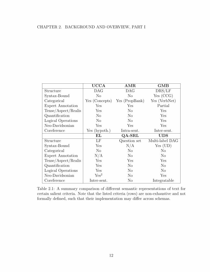
UCCA AMR GMBStructure DAG DAG DRS/LFSyntax-Bound No No Yes (CCG)Categorical Yes (Concepts) Yes (PropBank) Yes (VerbNet)Expert Annotation Yes Yes PartialTense/Aspect/Realis Yes No YesQuantification No No YesLogical Operations No No YesNeo-Davidsonian Yes Yes YesCoreference Yes (hypoth.) Intra-sent. Inter-sent.

EL QA-SRL UDSStructure LF Question set Multi-label DAGSyntax-Bound Yes N/A Yes (UD)Categorical No No NoExpert Annotation N/A No NoTense/Aspect/Realis Yes Yes YesQuantification Yes No NoLogical Operations Yes No NoNeo-Davidsonian Yes2 No YesCoreference Inter-sent. No Integratable

Table 2.1: A summary comparison of different semantic representations of text forcertain salient criteria. Note that the listed criteria (rows) are non-exhaustive and notformally defined, such that their implementation may differ across schemas.

12


labeling and event factuality prediction. In Part II of this thesis, we will turn to

the topic of script induction, or learning sequences of events from collections of

documents; since event representations in script induction have traditionally been

based on dependency syntax, we will employ the UDS parsers presented in Part I to

augment script event representations with UDS features and learn decompositional

scripts.

2In comparing Episodic Logic to neo-Davidsonian representations, Schubert and Hwang (2000)write “...while Davidson introduced event variables as ‘extra arguments’ of verbs, our approach(following (Reichenbach, 1947) ...) associates episodic variables with arbitrarily complex sentences.”

13

Chapter 3

Is the Universal Dependency

Representation Semantic?

The Universal Dependencies (UD) are a syntactic representation that inform the

structure of Universal Decompositional Semantic (UDS) representations (White et al.,

2016a). Specifically, in English UDS, a UD syntax parse is used to directly determine

a predicate-argument graph structure from the corresponding sentence; the nodes

(predicates and arguments) and edges (predicate-argument pairs) thereof are then

decorated with sets of independent semantic features. A natural question to ask

is: how much semantic information is already provided by the underlying syntactic

dependencies in this representation? In other words, are the additional semantic

features of UDS on top of syntax necessary? This question is further motivated by

the observation that syntactic dependency representations are often also regarded as

14

CHAPTER 3. IS THE UNIVERSAL DEPENDENCY REPRESENTATIONSEMANTIC?

shallow semantic representations (Schuster and Manning, 2016a; Hajicova, 1998).

In this chapter, we explore the extent to which meaningful semantic distinctions

are or are not captured by the Stanford Dependency representation (Marneffe and

Manning, 2008). Although the Stanford Dependencies and Universal Dependencies

are formally separate representation standards, they are similar in many regards. The

enhanced and enhanced++ versions of UD representations were introduced to capture

many of the conveniences of the collapsed Stanford Dependencies and basic UD parses

may be directly convered to enhanced/enhanced++ UD parses with a rule-based

conversion tool introduced by (Schuster and Manning, 2016a). Thus, although the

analysis presented in this chapter focuses on Stanford Dependencies, the conclusions

may generally be extended to UD representations as well.

To answer the central question of this chapter, we investigate the feasibility of

mapping Stanford dependency parses to Hobbsian Logical Form, a practical, event-

theoretic semantic representation, using only a set of deterministic rules. Although

we find that such a mapping is possible in a large number of cases, we also find cases

for which such a mapping seems to require information beyond what the Stanford

Dependencies encode. These cases shed light on the kinds of semantic information

that are and are not present in the Stanford Dependencies.

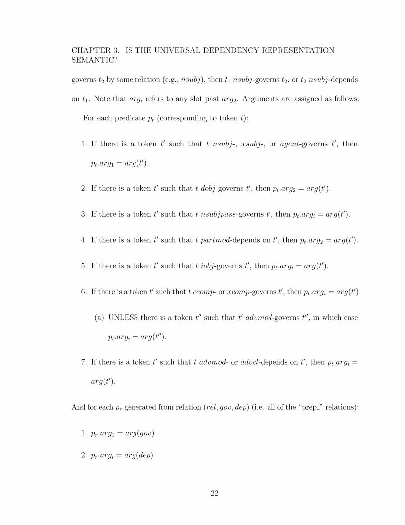
The deterministic rules for mapping dependency parses to HLFs presented herein

have formed the basis for the subsequent development of the predicate-argument

15


extraction system, PredPatt1, presented in White et al. (2016a).

3.1 Introduction

The Stanford dependency parser (De Marneffe, MacCartney, and Manning, 2006)

provides “deep” syntactic analysis of natural language by layering a set of hand-written

post-processing rules on top of Stanford’s statistical constituency parser (Klein and

Manning, 2003). Stanford dependency parses have been commonly used as a semantic

representation in natural language understanding and inference systems.2 For example,

they have been used as a basic meaning representation for the Recognizing Textual

Entailment task proposed by Dagan, Glickman, and Magnini (2005), such as by

Haghighi, Ng, and Manning (2005) and in other inference systems (Chambers et al.,

2007; MacCartney, 2009).

Because of their popular use as a semantic representation, it is important to

ask whether the Stanford Dependencies do, in fact, encode the kind of information

that ought to be present in a versatile semantic form. We address this question by

attempting to map the Stanford Dependencies into Hobbsian Logical Form (henceforth,

HLF), a neo-Davidsonian semantic representation designed for practical use (Hobbs,

1985). Our approach is to layer a set of hand-written rules on top of the Stanford

Dependencies to further transform the representation into HLFs. This approach is

1http://decomp.io/projects/predpatt/2Statement presented by Chris Manning at the *SEM 2013 Panel on Language Understanding

http://nlpers.blogspot.com/2013/07/the-sem-2013-panel-on-language.html.

16

http://decomp.io/projects/predpatt/


a natural extension of the Stanford Dependencies which were, themselves, originally

derived from manually engineered post-processing routines.

The aim of this chapter, then, is neither to demonstrate the semantic completeness

of the Stanford Dependencies, nor to exhaustively enumerate their semantic deficiencies.

Indeed, to do so would be to presuppose HLF as an entirely complete semantic

representation, or, a perfect semantic standard against which to compare the Stanford

Dependencies. We make no such claim. Rather, our intent is to provide a qualitative

discussion of the Stanford Dependencies as a semantic resource through the lens of this

HLF mapping task. It is only necessary that HLF capture some subset of important

semantic phenomena to make this exercise meaningful.

Our results indicate that in a number of cases, it is, in fact, possible to directly

derive HLFs from Stanford dependency parses. At the same time, however, we also

find difficult-to-map phenomena that reveal inherent limitations of the dependencies as

a meaning representation. In many cases, some of these deficiencies may be addressed

by one or more semantic property in a UDS representation.

3.2 Background

This section provides a brief overview of the HLF and Stanford dependency

formalisms.

17


Stanford Dependencies

A Stanford dependency parse is a set of triples consisting of two tokens (a governor

and a dependent), and a labeled syntactic or semantic relation between the two tokens.

Parses can be rendered as labeled, directed graphs, as in Figure 3.1. Note that here

we are using the collapsed version of the Stanford Dependencies.3

Figure 3.1: Stanford dependency parse of “A boy wants to build a boat quickly.”

Hobbsian Logical Form

The key insight of event-theoretic semantic representations is the reification of

events (Davidson, 1967a), or, treating events as entities in the world. As a logical,

first-order representation, Hobbsian Logical Form (Hobbs, 1985) employs this approach

by allowing for the reification of any predicate into an event variable. Specifically,

for any predicate p(x1, · · · , xn), there is a corresponding predicate, p′(E, x1, · · · , xn),

where E refers to the predicate (or event) p(x1, · · · , xn). The reified predicates are

3The collapsed version is more convenient for our purposes, but using the uncollapsed versionwould not significantly affect our results.

18


related to their non-reified forms with the following axiom schema:

(∀x1 · · ·xn)[p(x1 · · ·xn)↔ (∃e)Exist(e) ∧ p′(e, x1 · · ·xn)]

In HLF, “A boy runs” would be represented as:

(∃e, x)Exist(e) ∧ run′(e, x) ∧ boy(x)

and the sentence “A boy wants to build a boat quickly” (Hobbs, 1985) would be

represented as:

(∃e1, e2, e3, x, y)Exist(e1) ∧ want′(e1, x, e2)

∧quick′(e2, e3) ∧ build′(e3, x, y) ∧ boy(x) ∧ boat(y)

3.3 Mapping to HLF

We describe in this section our deterministic algorithm for mapping Stanford

dependency parses to HLF. The algorithm proceeds in four stages: event extraction,

argument identification, predicate-argument assignment, and formula construction. We

demonstrate these steps on the above example sentence “A boy wants to build a boat

quickly.”4 The rule-based algorithm operates on the sentence level and is purely a

4Hobbs (1985) uses the example sentence “A boy wanted to build a boat quickly.”

19


function of the dependency parse or other trivially extractible information, such as

capitalization.

Event Extraction

The first step is to identify the set of event predicates that will appear in the final

HLF and assign an event variable to each. Most predicates are generated by a single

token in the sentence (e.g., the main verb). For each token t in the sentence, an event

(ei, pt) (where ei is the event variable and pt is the predicate) is added to the set of

events if any of the following conditions are met:

1. t is the dependent of the relation root, ccomp, xcomp, advcl, advmod, or

partmod.

2. t is the governor of the relation nsubj, dobj, ccomp, xcomp, xsubj, advcl,

nsubjpass, or agent.

Furthermore, an event (ei, pr) is added for any triple (rel, gov, dep) where rel is

prefixed with “prep ” (e.g., prep to, prep from, prep by, etc.).

Applying this step to our example sentence “A boy wants to build a boat quickly.”

yields the following set:

(e1, wants), (e2, quickly), (e3, build)

20


Argument Identification

Next, the set of entities that will serve as predicate arguments are identified.

Crucially, this set will include some event variables generated in the previous step.

For each token, t, an argument (xi, t) is added to the set of arguments if one of the

following conditions is met:

1. t is the dependent of the relation nsubj, xsubj, dobj, ccomp, xcomp, nsubjpass,

agent, or iobj.

2. t is the governor of the relation advcl, advmod, or partmod.

Applying this step to our example sentence, we get the following argument set:

(x1, boat), (x2, build), (x3, boy)

Notice that the token build has generated both an event predicate and an argument.

This is because in our final HLF, build will be both an event predicate that takes the

arguments boy and boat, as well as an argument to the intensional predicate want.

Predicate-Argument Assignment

In this stage, arguments are assigned to each predicate. pt.argi denotes the ith

argument of predicate pt and arg(t) denotes the argument associated with token t.

For example, arg(boy) = x2 and arg(quickly) = e3. We also say that if the token t1

21


governs t2 by some relation (e.g., nsubj), then t1 nsubj-governs t2, or t2 nsubj-depends

on t1. Note that argi refers to any slot past arg2. Arguments are assigned as follows.

For each predicate pt (corresponding to token t):

1. If there is a token t′ such that t nsubj-, xsubj-, or agent-governs t′, then

pt.arg1 = arg(t′).

2. If there is a token t′ such that t dobj-governs t′, then pt.arg2 = arg(t′).

3. If there is a token t′ such that t nsubjpass-governs t′, then pt.argi = arg(t′).

4. If there is a token t′ such that t partmod-depends on t′, then pt.arg2 = arg(t′).

5. If there is a token t′ such that t iobj-governs t′, then pt.argi = arg(t′).

6. If there is a token t′ such that t ccomp- or xcomp-governs t′, then pt.argi = arg(t′)

(a) UNLESS there is a token t′′ such that t′ advmod-governs t′′, in which case

pt.argi = arg(t′′).

7. If there is a token t′ such that t advmod- or advcl-depends on t′, then pt.argi =

arg(t′).

And for each pr generated from relation (rel, gov, dep) (i.e. all of the “prep ” relations):

1. pr.arg1 = arg(gov)

2. pr.argi = arg(dep)

22


After running this stage on our example sentence, the predicate-argument assign-

ments are as follows:

wants(x3, e2), build(x3, x1), quickly(e3)

Each predicate can be directly replaced with its reified forms (i.e., p′):

wants′(e1, x3, e2), build′(e3, x3, x1), quickly

′(e2, e3)

Two kinds of non-eventive predicates still need to be formed. First, every entity

(xi, t) that is neither a reified event nor a proper noun, e.g., (x3, boy), generates a

predicate of the form t(xi). Second, we generate Hobbs’s Exist predicate, which

identifies which event actually occurs in the “real world.” This is simply the event

generated by the dependent of the root relation.

Formula Construction

In this stage, the final HLF is pieced together. We join all of the predicates formed

above with the and conjunction, and existentially quantify over every variable found

therein. For our example sentence, the resulting HLF is:

23


A boy wants to build a boat quickly.

(∃e1, e2, e3, x1, x3)[Exist(e1) ∧ boat(x1) ∧ boy(x3) ∧ wants′(e1, x3, e2)

∧build′(e3, x3, x1) ∧ quickly′(e2, e3)]

3.4 Analysis of Results

This section discusses semantic phenomena that our mapping does and does not

capture, providing a lens for assessing the usefulness of the Stanford Dependencies as

a semantic resource.

Successes

Formulas 3.1-3.7 are correct HLFs that our mapping rules successfully generate.

They illustrate the diversity of semantic information that is easily recoverable from

Stanford dependency parses.

Formulas 3.1-3.2 show successful parses in simple transitive sentences with ac-

tive/passive alternations, and Formula 3.3 demonstrates success in parsing ditransitives.

Also easily recovered from the dependency structures are semantic parses of sentences

with adverbs (Formula 3.4) and reporting verbs (Formula 3.5). Lest it appear that

these phenomena may only be handled in isolation, Equations 3.6-3.7 show successful

24


parses for sentences with arbitrary combinations of the above phenomena.

A boy builds a boat.

(∃e1, x1, x2)[Exist(e1) ∧ boy(x2) ∧ boat(x1) ∧ builds′(e1, x2, x1)]

(3.1)

A boat was built by a boy.

(∃e1, x1, x2)[Exist(e1) ∧ boat(x2) ∧ boy(x1) ∧ built′(e1, x1, x2)]

(3.2)

Jackie gave Morgan a boat.

(∃e1, x1)[Exist(e1) ∧ boat(x1) ∧ gave′(e1, Jackie, x1,Morgan)]

(3.3)

Jackie built a boat quickly. OR Jackie quickly built a boat.

(∃e1, e2, x1)[Exist(e1) ∧ boat(x1) ∧ quickly(e2, e1) ∧ built′(e1, Jackie, x1)]

(3.4)

25


Jackie told Morgan that a boy built a boat.

(∃e1, e2, x1, x4)[Exist(e1) ∧ boy(x1) ∧ boat(x4) ∧ built′(e2, x1, x4) ∧

told′(e1, Jackie,Morgan, e2)]

(3.5)

Jackie told Morgan that Sam told Jesse that Alex loves Pat.

(∃e1, e2, e3)[Exist(e1) ∧ told′(e2, Sam, Jesse, e3) ∧ loves′(e3, Alex, Pat) ∧

told′(e1, Jackie,Morgan, e2)]

(3.6)

Jackie was told by Morgan that Sam wants Jesse to build a boat quickly.

(∃e1, e2, e3, e4, x7)[Exist(e1) ∧ boat(x7) ∧ build′(e2, Jesse, x7) ∧

told′(e1,Morgan, Jackie, e4) ∧ wants′(e4, Sam, e3) ∧ quickly′(e3, e2)]

(3.7)

Limitations

Though our mapping rules enable us to directly extract deep semantic information

directly from the Stanford dependency parses in the above cases, there are a number

26


of difficulties with this approach that shed light on inherent limitations of the Stanford

Dependencies as a semantic resource.

A major such limitation arises in cases of event nominalizations. Because depen-

dency parses are syntax-based, their structures do not distinguish between eventive

noun phrases like “the bombing of the city” and non-eventive ones like “the mother of

the child”; such a distinction, however, would be found in the corresponding HLFs.

Certain syntactic alternations also prove problematic. For example, the dependency

structure does not recognize that “window” takes the same semantic role in the

sentences “Jackie broke the mirror.” and “The mirror broke.” The use of additional

semantic lables, like PropBank role labels (Palmer, Gildea, and Kingsbury, 2005b),

would be necessary to determine this. Specific semantic proto-role properties in the

UDS representation, like changed-state or destroyed would also enable this

distinction. These properties will be introduced in greater detail in Chapters 4 and 5.

Prepositional phrases present another problem for our mapping task, as the

Stanford dependencies will typically not distinguish between PPs indicating arguments

and adjuncts. For example, “Morgan stuffed envelopes with coupons” and “Morgan

stuffed envelopes with Jackie” have identical dependency structures, yet “coupons”

and “Jackie” are (hopefully for Jackie) taking on different semantic roles. This is,

in fact, a prime example of how Stanford dependency parses may resolve syntactic

ambiguity without resolving semantic ambiguity. In this case as well, a UDS proto-role

property like changed-location might enable such a distinction to be drawn.

27


One additional semantic limitation of the syntactic dependency representation is

that it does not give us insight into certain lexical entailments with regard to the

embedded predicates of clause-embedding verbs. For example, there is no difference

between the Stanford dependency parses of the sentences “A boy managed to build a

boat” and “A boy failed to build a boat.”; in the former sentence, the building event

happened, and in the latter, it did not. This could be distinguished in HLF by the use

of the Exist predicate. In UDS, the semantic property factual (which decorates

a predicate node) would also make this distinction. This detection of a predicate or

event’s factuality will be the subject of Chapter 5.

Of course, one might manage more HLF coverage by adding more rules to our

system, but the limitations discussed here are fundamental. If two sentences have

different semantic interpretations but identical dependency structures, then there can

be no deterministic mapping rule (based on dependency structure alone) that yields

this distinction.

3.5 Conclusion

We have presented here an attempt to map the Stanford Dependencies to HLF

via a second layer of hand-written rules. That our mapping rules, which are purely a

function of dependency structure, succeed in producing correct HLFs in some cases

is good evidence that the Stanford Dependencies do contain some practical level of

semantic information. Nevertheless, we were also able to quickly identify aspects of

28


meaning that the Stanford Dependencies do not capture.

Our argument does not require that HLF be an optimal representation, only that

it capture worthwhile aspects of semantics and that it not be readily derived from the

Stanford representation. This is enough to conclude that the Stanford Dependencies,

and by extension, the English Universal Dependencies, are not sufficient in all cases

as a meaning representation. This observation motivates the next two chapters of this

thesis, in which we will investigate two types of semantic features that decorate UDS

structures: semantic proto-role labels (Chapter 4) and event factuality (Chapter 5).

29

Chapter 4

Neural-Davidsonian Semantic

Proto-Role Labeling

In Chapter 3, we noted that dependency syntax, while useful in identifying the

underlying predicate-argument structure of HLF, does not capture every distinction

we may wish to denote in a semantic representation. Accordingly, we may think of

Universal Decompositional Semantics (UDS) (White et al., 2016a) as consisting of

predicate-argument structures determined by syntax1 and decorated with many layers

of independent semantic features. Chief among these semantic layers are semantic

proto-role properties (Reisinger et al., 2015).

In this chapter, we present a novel model for the prediction of semantic proto-

role properties (SPRL) that achieves high accuracy. Specifically, this model uses an

1Indeed, the predicate-argument extraction toolkit, PredPatt, which determines the underlyingstructure of UDS, is an outgrowth of the mapping rules outlined in Chapter 3.

30

CHAPTER 4. NEURAL-DAVIDSONIAN SEMANTIC PROTO-ROLE LABELING

adapted bidirectional long short-term memory network (LSTM) encoding strategy

that we call Neural-Davidsonian: predicate-argument structure is represented as pairs

of hidden states corresponding to predicate and argument head tokens of the input

sequence. We demonstrate: (1) state-of-the-art results in SPRL, and (2) that our

network naturally shares parameters between attributes, allowing for learning new

attribute types with limited added supervision.

4.1 Introduction

Universal Decompositional Semantics (UDS) (White et al., 2016a) is a contem-

porary semantic representation of text (Abend and Rappoport, 2017) that forgoes

traditional inventories of semantic categories in favor of bundles of simple, interpretable

properties. In particular, UDS includes a practical implementation of Dowty’s theory

of thematic proto-roles (Dowty, 1991): arguments are labeled with properties typical

of Dowty’s proto-agent (awareness, volition ...) and proto-patient (changed

state ...).

Annotated corpora have allowed the exploration of Semantic Proto-role Labeling

(SPRL) 2 as a natural language processing task (Reisinger et al., 2015; White et al.,

2016a; Teichert et al., 2017). For example, consider the following sentence, in which a

particular pair of predicate and argument heads have been emphasized: “The cat ate

the rat.” An SPRL system must infer from the context of the sentence whether the

2SPRL and SPR refer to the labeling task and the underlying semantic representation, respectively.

31


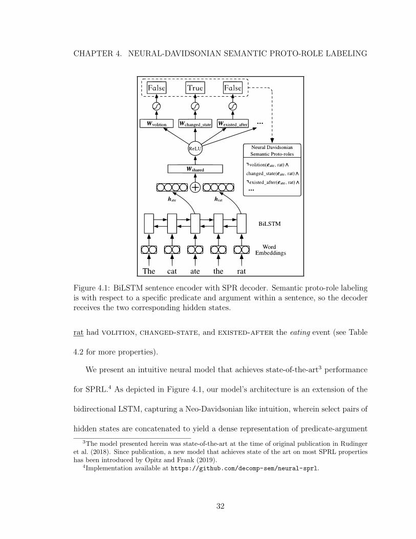
Figure 4.1: BiLSTM sentence encoder with SPR decoder. Semantic proto-role labelingis with respect to a specific predicate and argument within a sentence, so the decoderreceives the two corresponding hidden states.

rat had volition, changed-state, and existed-after the eating event (see Table

4.2 for more properties).

We present an intuitive neural model that achieves state-of-the-art3 performance

for SPRL.4 As depicted in Figure 4.1, our model’s architecture is an extension of the

bidirectional LSTM, capturing a Neo-Davidsonian like intuition, wherein select pairs of

hidden states are concatenated to yield a dense representation of predicate-argument

3The model presented herein was state-of-the-art at the time of original publication in Rudingeret al. (2018). Since publication, a new model that achieves state of the art on most SPRL propertieshas been introduced by Opitz and Frank (2019).

4Implementation available at https://github.com/decomp-sem/neural-sprl.

32

https://github.com/decomp-sem/neural-sprl


SPR Property Explanation of Property

instigation Arg caused the Pred to happen? yes novolitional Arg chose to be involved in the Pred? yes no

awareArg was/were aware of beinginvolved in the Pred?

yes yes

physically existed Arg existed as a physical object? yes yesexisted after Arg existed after the Pred stopped? yes no

changed stateThe Arg was/were altered or somehowchanged during or by the end of the Pred?

yes yes

Table 4.1: Example SPR annotations for the toy example “The cat ate the rat,”where the Predicate in question is “ate” and the Argument in question is either “cat”or “rat.” Note that not all SPR properties are listed, and the binary labels (yes, no)are coarsened from a 5-point Likert scale.

structure and fed to a prediction layer for end-to-end training. We include a thorough

quantitative analysis highlighting the contrasting errors between the proposed model

and previous (non-neural) state-of-the-art.

In addition, our network naturally shares a subset of parameters between attributes.

We demonstrate how this allows learning to predict new attributes with limited

supervision: a key finding that could support efficient expansion of new SPR attribute

types in the future.

4.2 Background

Davidson (1967b) is credited for representations of meaning involving propositions

composed of a fixed arity predicate, all of its core arguments arising from the natural

language syntax, and a distinguished event variable. The earlier example could thus be

33


denoted (modulo tense) as (∃e)eat[(e,cat,rat)], where the variable e is a reification of

the eating event. The order of the arguments in the predication implies their role, where

leaving arguments unspecified (as in “The cat eats”) can be handled either by introduc-

ing variables for unstated arguments, e.g., (∃e)(∃x)[eat(e,cat, x)], or by creating new

predicates that correspond to different arities, e.g., (∃e)eat intransitive[(e,cat)].5

The Neo-Davidsonian approach (Castaneda, 1967; Parsons, 1995), which we follow

in this work, allows for variable arity by mapping the argument positions of individ-

ual predicates to generalized semantic roles, shared across predicates,6 e.g., agent,

patient and theme, in: (∃e)[eat(e) ∧Agent(e,cat) ∧Patient(e,rat)].

Dowty (1991) conjectured that the distinction between the role of a prototypical

Agent and prototypical Patient could be decomposed into a number of semantic

properties such as “Did the argument change state?”; these semantic distinctions then

serve to determine the syntactic position assigned to each argument of a predicate

in its surface realization. Here we formulate a Neo-Davidsonian event representation

employing Dowty-inspired semantic proto-role (SPR) attributes:

(∃e) [eat(e)

∧ volition(e,cat) ∧ instigation(e,cat)...

∧ ¬volition(e,rat) ∧ destroyed(e,rat)... ]

5This formalism aligns with that used in PropBank (Palmer, Gildea, and Kingsbury, 2005a),which associated numbered, core arguments with each sense of a verb in their corpus annotation.

6For example, as seen in FrameNet (Baker, Fillmore, and Lowe, 1998).

34


Dowty’s theory was empirically verified by Kako (2006), followed by pilot (Mad-

nani, Boyd-Graber, and Resnik, 2010) and large-scale (Reisinger et al., 2015) corpus

annotation efforts, the latter introducing a logistic regression baseline for SPRL. Te-

ichert et al. (2017) refined the evaluation protocol,7 and developed a CRF (Lafferty,

McCallum, and Pereira, 2001) for the task, representing existing state-of-the-art.

Full details about the SPR datasets introduced by Reisinger et al. (2015) and

White et al. (2016a), which we use in this work, are provided in Section 4.4. For

clarity, Table 4.1 shows a toy SPRL example, including a few sample SPR properties

and explanations.

4.3 “Neural-Davidsonian” Model

Our proposed SPRL model (Fig. 4.1) determines the value of each attribute (e.g.,

volition) on an argument (a) with respect to a particular predication (e) as a

function on the latent states associated with the pair, (e, a), in the context of a full

sentence. Our architecture encodes the sentence using a shared, one-layer, bidirectional

LSTM (Hochreiter and Schmidhuber, 1997b; Graves, Jaitly, and Mohamed, 2013),

or, BiLSTM. We then obtain a continuous, vector representation hea = [he;ha], for

each predicate-argument pair as the concatenation of the hidden BiLSTM states he

and ha corresponding to the syntactic head of the predicate of e and argument a

7Splitting train/dev/test along Penn Treebank boundaries and casting the SPRL task as multi-labelbinary classification.

35


respectively. These heads are obtained over gold syntactic parses using the predicate-

argument detection tool, PredPatt (White et al., 2016a).8 We note here related work

in semantic role labeling by He et al. (2018) which also treats predicate-argument

pairs independntly and thus could also be considered “neural-Davidsonian” under

this formulation; a key difference is that here we consider the syntactic head of the

argument where He et al. (2018) instead consider the argument’s span.

For each SPR attribute, a score is predicted by passing hea through a separate

two-layer perceptron, with the weights of the first layer shared across all attributes:

Score(attr,hea) = Wattr [g (Wshared [hea])]

This architecture accommodates the definition of SPRL as multi-label binary

classification given by Teichert et al. (2017) by treating the score as the log-odds of the

attribute being present (i.e. P(attr|hea) = 11+exp[−Score(attr,hea)]

). This architecture also

supports SPRL as a scalar regression task where the parameters of the network are

tuned to directly minimize the discrepancy between the predicted score and a reference

scalar label. The loss for the binary and scalar models are negative log-probability

and squared error, respectively; the losses are summed over all SPR attributes.

Training with Auxiliary Tasks A benefit of the shared neural-Davidsonian repre-

sentation is that it offers many levels at which multi-task learning may be leveraged to

8Observed to be state-of-the-art by Zhang, Rudinger, and Van Durme (2017).

36


improve parameter estimation so as to produce semantically rich representations hea,

he, and ha. For example, the sentence encoder might be pre-trained as an encoder

for machine translation, the argument representation ha can be jointly trained to

predict word-sense, the predicate representation, he, could be jointly trained to predict

factuality (Saurı and Pustejovsky, 2009; Rudinger, White, and Van Durme, 2018), and

the predicate-argument representation, hea, could be jointly trained to predict other

semantic role formalisms (e.g. PropBank SRL—suggesting a neural-Davidsonian SRL

model in contrast to recent BIO-style neural models of SRL (He et al., 2017)).

To evaluate this idea empirically, we experimented with a number of multi-task

training strategies for SPRL. While all settings outperformed prior work in aggregate,

simply initializing the BiLSTM parameters with a pretrained English-to-French ma-

chine translation encoder9 produced the best results,10 so we simplify discussion by

focusing on that model. The efficacy of MT pretraining that we observe here comes as

no surprise given prior work demonstrating, e.g., the utility of bitext for paraphrase

(Ganitkevitch, Van Durme, and Callison-Burch, 2013), that NMT pretraining yields

improved contextualized word embeddings11 (McCann et al., 2017), and that NMT

encoders specifically capture useful features for SPRL (Poliak et al., 2018b). Full

details about each multi-task experiment, including a full set of ablation results, are

9using a modified version of OpenNMT-py (Klein et al., 2017) trained on the 109 Fr-En corpus(Callison-Burch et al., 2009) (Section 4.6).

10e.g. this initialization resulted in raising micro-averaged F1 from 82.2 to 83.311More recent discoveries on the usefulness of language model pretraining (Peters et al., 2018;

Howard and Ruder, 2018) for RNN encoders suggest a promising direction for future SPRL experi-ments.

37


reported in Section 4.6; details about the corresponding datasets are in Section 4.4.

Except in the ablation experiment of Figure 4.2, our model was trained on only

the SPRL data and splits used by Teichert et al. (2017) (learning all properties

jointly), using GloVe12 embeddings and with the MT-initialized BiLSTM. Models were

implemented in PyTorch and trained end-to-end with Adam optimization (Kingma

and Ba, 2014) and a default learning rate of 10−3. Each model was trained for ten

epochs, selecting the best-performing epoch on dev.

Prior Work in SPRL We additionally include results from prior work: “lr” is the

logistic-regression model introduced by Reisinger et al. (2015) and “crf” is the CRF

model (specifically SPRL⋆) from Teichert et al. (2017). Although White et al. (2016a)

released additional SPR annotations, we are unaware of any benchmark results on

that data; however, our multi-task results in Section 4.6 do use the data and we find

(unsurprisingly) that concurrent training on the two SPR datasets can be helpful.

Using only data and splits from White et al. (2016a), the scalar regression architecture

of Table 4.6 achieves a Pearson’s ρ of 0.577 on test.

There are a few noteworthy differences between our neural model and the CRF

of prior work. As an adapted BiLSTM, our model easily exploits the benefits of

large-scale pretraining, in the form of GloVe embeddings and MT pretraining, both

absent in the CRF. Ablation experiments (Section 4.6) show the advantages conferred

12300-dimensional, uncased; glove.42B.300d from https://nlp.stanford.edu/projects/

glove/; 15,533 out-of-vocabulary words across all datasets were assigned a random embedding(uniformly from [−.01, .01]). Embeddings remained fixed during training.

38

https://nlp.stanford.edu/projects/glove/

https://nlp.stanford.edu/projects/glove/


by these features. In contrast, the discrete-featured CRF model makes use of gold

dependency labels, as well as joint modeling of SPR attribute pairs with explicit joint

factors, both absent in our neural model. Future SPRL work could explore the use of

models like the LSTM-CRF (Lample et al., 2016; Ma and Hovy, 2016) to combine the

advantages of both paradigms.

4.4 Data

Here we describe each dataset used in training the “Neural-Davidsonian” SRPL

model. The SPR1 and SPR2 datasets are the primary datasets of focus. The

subsequent datasets are used for auxiliary tasks in the multi-task training experiments,

described in Section 4.6.

SPR1

The SPR1.0 (“SPR1”) dataset introduced by Reisinger et al. (2015) contains

proto-role annotations on 4,912 Wall Street Journal sentences from PropBank (Palmer,

Gildea, and Kingsbury, 2005a) corresponding to 9,738 predicate-argument pairs with

18 properties each, in total 175,284 property annotations. All annotations were

performed by a single, trusted annotator. Each annotation is a rating from 1 to 5

indicating the likelihood that the property applies, with an additional “N/A” option

if the question of whether the property holds is nonsensical in the context.

To compare with prior work (Teichert et al., 2017), we treat the SPR1 data as

39


a binary prediction task: the values 4 and 5 are mapped to True (property holds),

while the values 1, 2, 3, and “N/A” are mapped to False (property does not hold).

In additional experiments, we move to treating SPR1 as a scalar prediction task; in

this case, “N/A” is mapped to 1, and all other annotation values remain unchanged.

SPR2

The second SPR release (White et al., 2016a) contains annotations on 2,758

sentences from the English Web Treebank (EWT) (Bies et al., 2012) portion of

the Universal Dependencies (v1.2) (Silveira et al., 2014)13, corresponding to 6,091

predicate-argument pairs. With 14 proto-role properties each, there are a total

of 85,274 annotations, with two-way redundancy. As in SPR1, the value of each

annotation is an integral value 1-5 or “N/A.” We treat SPR2 as a scalar prediction

task, first mapping “N/A” to 1, and then averaging the two-way redundant annotation

values to a single value.

Word Sense Disambiguation

Aligned with proto-role property annotations in the SPR2 release are word sense

disambiguation judgments for the head tokens of arguments. Candidate word senses

(fine-grained) from WordNet (Fellbaum, 1998) were presented to Mechanical Turk

workers (at least three annotators per instance), who selected every applicable sense

13We exclude the SPR2 pilot data; if included, the SPR2 release contains annotations for 2,793sentences.

40


of the word in the given context. In this work, we map the fine-grained word senses to

one of 26 coarse-grained WordNet noun supersenses (e.g., noun.animal, noun.event,

noun.quantity, etc.). In many cases, a word may be mapped to more than one

supersense. We treat the supersense label on a word as a distribution over supersenses,

where the probability assigned to one supersense is proportional to the number of

annotators that (indirectly) selected that supersense. In practice, the entropy of these

resulting supersense distributions is low, with an average perplexity of 1.42.

PropBank

The PropBank project consists of predicate-argument annotations over corpora

for which gold Penn TreeBank-style constituency parses are available. We use the

Unified PropBank release (Bonial et al., 2014; Ide and Pustejovsky, 2017), which

contains annotations over OntoNotes as well as the English Web TreeBank (EWT).

Each predicate in each corpus is annotated for word sense, and each argument of

each predicate is given a label such as ARG0, ARG1, etc., where the interpretation

of the label is defined relative to the word sense. We use PropBank Frames to map

these sense-specific labels to 16 sense-independent labels such as PAG (proto-agent),

PPT (proto-patient), etc., and then formulate a task to predict the abstracted labels.

Because our model requires knowledge of predicate and argument head words, we

ran the Stanford Universal Dependencies converter (Schuster and Manning, 2016b)

over the gold constituency parses to obtain Universal Dependency parses, which were

41


then processed by the PredPatt framework (Zhang, Rudinger, and Van Durme, 2017;

White et al., 2016a) to identify head words.

English-French Data

The 109 French-English parallel corpus (Callison-Burch et al., 2009) contains

22,520,376 French-English sentence pairs, made up of 811,203,407 French words and

668,412,817 English words. The corpus was constructed by crawling the websites of

international organizations such as the Canadian government, the European Union,

and the United Nations.

4.5 Experiments

Table 4.2 shows a side-by-side comparison of our model with prior work. The full

breakdown of F1 scores over each individual property is provided. For every property

except existed during, existed after, and created we are able to exceed prior

performance. For some properties, the absolute F1 gains are quite large: destroyed

(+24.2), changed possession (+19.2.0), changed location (+10.1), stationary

(+26.0) and location (+35.3). We also report performance with a scalar regression

version of the model, evaluated with Pearson correlation. The scalar model is with

respect to the original SPR annotations on a 5-point Likert scale, instead of a binary

cut-point along that scale (> 3).

Manual Analysis We select two properties (volition and makes physical

42


previous work this worklr crf binary scalar

instigation 76.7 85.6 88.6 0.858volition 69.8 86.4 88.1 0.882awareness 68.8 87.3 89.9 0.897sentient 42.0 85.6 90.6 0.925physically existed 50.0 76.4 82.7 0.834existed before 79.5 84.8 85.1 0.710existed during 93.1 95.1 95.0 0.673existed after 82.3 87.5 85.9 0.619created 0.0 44.4 39.7 0.549destroyed 17.1 0.0 24.2 0.346changed 54.0 67.8 70.7 0.592changed state 54.6 66.1 71.0 0.604changed possession 0.0 38.8 58.0 0.640changed location 6.6 35.6 45.7 0.702stationary 13.3 21.4 47.4 0.711location 0.0 18.5 53.8 0.619physical contact 21.5 40.7 47.2 0.741manipulated 72.1 86.0 86.8 0.737

micro f1 71.0 81.7 83.3macro f1 55.4⋆ 65.9⋆ 71.1macro-avg pearson 0.753

Table 4.2: SPR comparison to Teichert et al. (2017). Bold number indicate best F1results in each row. Right-most column is pearson correlation coeficient for a modeltrained and tested on the scalar regression formulation of the same data.

contact) to perform a manual error analysis with respect to crf 14 and our binary

model from Table 4.2. For each property, we sample 40 dev instances with gold labels

of “True” (> 3) and 40 instances of “False” (≤ 3), restricted to cases where the two

system predictions disagree.15 We manually label each of these instances for the six

features shown in Table 4.3. For example, given the input “He sits down at the piano

14We obtained the crf dev system predictions of Teichert et al. (2017) via personal communicationwith the authors.

15According to the reference, of the 1071 dev examples, 150 have physical contact and 350 havevolition. The two models compared here differed in phy. contact on 62 positive and 44 negativeinstances and for volition on 43 positive and 54 negative instances.

43


phys. contact volition

#Differ

∆False

–

∆False

+

#Differ

∆False

–

∆False

+

1 All 80 −14 6 80 −14 −102 ProperNoun 18 −2 −2 21 4 −53 Org. 15 −9 2 31 −6 −14 Pronoun 10 0 8 12 0 0

5 PhraseVerb 14 −6 0 9 −4 1

6 Metaphor 11 −5 −2 6 −2 0

7 LightVerb 5 −2 1 5 −1 2

Table 4.3: Manual error analysis on a sample of instances (80 for each property) whereoutputs of crf and the binary model from Table 4.2 differ. Negative ∆ False+and ∆ False– indicate the neural model represents a net reduction in type I andtype II errors respectively over crf. Positive values indicate a net increase in errors.Each row corresponds to one of several (overlapping) subsets of the 80 instances indisagreement: (1) all (sampled) instances; (2) argument is a proper noun; (3) argumentis an organization or institution; (4) argument is a pronoun; (5) predicate is phrasalor a particle verb construction; (6) predicate is used metaphorically; (7) predicate is alight-verb construction. #Differ is the size of the respective subset.

and plays,” our neural model correctly predicts that He makes physical contact during

the sitting, while crf does not. Since He is a pronoun, and sits down is phrasal, this

example contributes −1 to ∆ False– in rows 1, 4 and 5.

For both properties our model appears more likely to correctly classify the argument

in cases where the predicate is a phrasal verb. This is likely a result of the fact that

the BiLSTM has stronger language-modeling capabilities than the crf, particularly

with MT pretraining. In general, our model increases the false-positive rate for makes

physical contact, but especially when the argument is pronominal.

44


●

●

●

● ●

●

●●

●

●

●

●

instigation manipulated

0 25 50 75 100 0 25 50 75 100

72

76

80

84

% of training data for property

F1

● all properties

target property only

Figure 4.2: Effect of using only a fraction of the training data for a property whileeither ignoring or co-training with the full training data for the other SPR1 properties.Measurements at 1%, 5%, 10%, 25%, 50%, and 100%.

Learning New SPR Properties One motivation for the decompositional approach

adopted by SPRL is the ability to incrementally build up an inventory of annotated

properties according to need and budget. Here we investigate (1) the degree to which

having less training data for a single property degrades our F1 for that property on

held-out data and (2) the effect on degradation of concurrent training with the other

properties. We focus on two properties only: instigation, a canonical example of a

proto-agent property, and manipulated, which is a proto-patient property. For each

we consider six training set sizes (1, 5, 10, 25, 50 and 100 percent of the instances).

Starting with the same randomly initialized BiLSTM16, we consider two training

scenarios: (1) ignoring the remaining properties or (2) including the model’s loss on

16Note that this experiment does not make use of MT pretraining as was used for Table 4.2, tobest highlight the impact of parameter sharing across attributes.

45


other properties with a weight of λ = 0.1 in the training objective.

Results are presented in Figure 4.2. We see that, in every case, most of the

performance is achieved with only 25% of the training data. The curves also suggest

that training simultaneously on all SPR properties allows the model to learn the

target property more quickly (i.e., with fewer training samples) than if trained on

that property in isolation. For example, at 5% of the training training data, the

“all properties” models are achieving roughly the same F1 on their respective target

property as the “target property only” models achieves at 50% of the data.17 As the

SPR properties currently annotated are by no means semantically exhaustive,18 this

experiment indicates that future annotation efforts may be well served by favoring

breadth over depth, collecting smaller numbers of examples for a larger set of attributes.

4.6 Mult-Task Investigation

Multi-task learning has been found to improve performance on many NLP tasks,

particularly for neural models, and is rapidly becoming de rigueur in the field. The

strategy involves optimizing for multiple training objectives corresponding to different

(but usually related) tasks. Collobert and Weston (2008) use multi-task learning

to train a convolutional neural network to perform multiple core NLP tasks (POS

17As we observed the same trend more clearly on the dev set, we suspect some over-fitting to thedevelopment data which was used for independently select a stopping epoch for each of the plottedpoints.

18E.g., annotations do not include any questions relating to the origin or destination of an event.

46


Name # Description

lr Logistic Regr. model,Reisinger et al. (2015)

crf CRF model,Teichert et al. (2017)

spr1 0 SPR1 basic modelspr1-rand 0 spr1, random word embeddingsmt:spr1 1a spr1 after MT pretrainingpb:spr1 1a spr1 after PB pretrainingmt:pb:spr1 1a spr1 after MT+PB pretrainingspr1+2 1b SPR1 and SPR2 concurrentlyspr1+wsd 1b SPR1 and WSD concurrentlymt:spr1+2 1b spr1+2 after MT pretrainingmt:spr1+wsd 1b spr1+wsd after MT pretrainingmt:spr1s 1c SPR1 scalar after MT pretrainingpb:spr1s 1c SPR1 scalar after PB pretrainingps-ms 1d SPR1 propty-specific model sel.spr2 2 SPR2 basic scalar modelmt:spr2 2 spr2 after MT pretrainingpb:spr2 2 spr2 after PB pretrainingmt:pb:spr2 2 spr2 after MT+PB pretraining

Table 4.4: Name and short description of each experimental condition reported;numbering corresponds to experiment numbers reported in Section 4.6.2. mt: indicatespretraining with machine translation; pb: indicates pretraining with PropBank SRL.

tagging, named entity recognition, etc.). Multi-task learning has also been used to

improve sentence compression (Klerke, Goldberg, and Søgaard, 2016), chunking and

dependency parsing (Hashimoto, Tsuruoka, and Socher, 2017). Related work on

UDS (White et al., 2016a) shows improvements on event factuality prediction with

multi-task learning on BiLSTM models (Rudinger, White, and Van Durme, 2018).

Expanding upon the basic experiments presented in the previous section, here we

perform an extensive investigation of the impact of multi-task learning for SPRL.

We borrow insights from Mou et al. (2016) who explore different multi-task

47


strategies for NLP including approach of initializing a network by training it on a

related task (“INIT”) versus interspersing tasks during training (“MULT”). Here

we employ both of these strategies, referring to them as pretraining and concurrent

training. We also use the terminology target task and auxiliary task to differentiate

the primary task(s) we are interested in from those that play only a supporting role in

training. In order to tune the impact of auxiliary tasks on the learned representation,

Luong et al. (2016) use a mixing parameter, αi, for each task i. Each parameter update

consists of selecting a task with probability proportional to its αi and then performing

one update with respect to that task alone. They show that the choice of α has a

large impact on the effect of multi-task training, which influences our experiments

here.

Please refer to Section 4.4 for details on the datasets used in this section. In

particular, with a few exceptions, White et al. (2016a) annotates for the same set

of properties as Reisinger et al. (2015), but with slightly different protocol and on

a different genre. However, in this section we treat the two datasets as if they were

separate tasks. To avoid cluttering the results in the main text, we exclusively present

results there on what we call SPR1 which consists of the data from Reisinger et al.

(2015) and the train/dev/test splits of Teichert et al. (2017). We refer to the analogous

tasks built on the data and splits of White et al. (2016a) using the term SPR2. (We

are not aware of any prior published results on property prediction for the SPR2.)

In addition to the binary and scalar SPR architectures outlined in Section 4.3,

48


we also considered concurrently training the BiLSTM on a fine-grained word-sense

disambiguation task or on joint SPR1 and SPR2 prediction. We also experimented

with using machine translation and PropBank SRL to initialize the parameters of the

BiLSTM. Preliminary experimentation on dev data with other combinations helped

prune down the set of interesting experiments to those listed in Table 4.4 which

assigns names to the models explored here. Our ablation study in Section 4.5 uses

the model named spr1 while the other results correspond to mt:spr1 in the case

of binary prediction and mt:spr1s in the case of scalar prediction. After detailing

the additional components used for pretraining or concurrent training, we present

aggregate results and for the best performing models (according to dev) we present

property-level aggregate results.

4.6.1 Auxiliary Tasks

Each auxiliary task is implemented in the form of a task-specific decoder with

access to the hidden states computed by the shared BiLSTM encoder. In this way,

the losses from these tasks backpropagate through the BiLSTM. Here we describe

each task-specific decoder.

PropBank Decoder

The network architecture for the auxiliary task of predicting abstract role types

in PropBank is nearly identical to the architecture for SPRL described in Section

49


4.3. The main difference is that the PropBank task is a single-label, categorical

classification task.

P(rolei|hea) = softmaxi (Wpropbank [hea])

The loss from this decoder is the negative log of the probability assigned to the

correct label.

Supersense Decoder

The word sense disambiguation decoder computes a probability distribution over

26 WordNet supersenses with a simple single-layer feedforward network:

P(supersensei|ha) = softmaxi(W [ha])

where W ∈ R1200×26 and ha is the RNN hidden state corresponding to the argument

head token we wish to disambiguate. Since the gold label in the supersense prediction

task is a distribution over supersenses, the loss from this decoder is the cross-entropy

between its predicted distribution and the gold distribution.

French Translation Decoder

Given the encoder hidden states, the goal of translation is to generate the reference

sequence of tokens Y = y1, · · · , yn in the target language, i.e., French. We employ the

50


standard decoder architecture for neural machine translation. At each time step i, the

probability distribution of the decoded token yi is defined as:

P (yi) = softmax(tanh(Wfr

[si; ci

]+ bfr)

)

where Wfr is a transform matrix, and bfr is a bias. The inputs are the decoder hidden

state si and the context vector ci. The decoder hidden state si is computed by:

si = rnn(yi−1, si−1)

where rnn is a recurrent neural network using L-layer stacked LSTM, yi−1 is the

word embedding of token yi−1, and s0 is initialized by the last encoder left-to-right

hidden state.

The context vector ci is computed by an attention mechanism (Bahdanau, Cho,

and Bengio, 2014; Luong, Pham, and Manning, 2015),

ci =∑t

αi,tht,

αi,t =exp

(s⊤i (Wαht + bα)

))∑

k exp(s⊤i (Wαhk + bα)

) ,where Wα is a transform matrix and bα is a bias. The loss is the negative log-

probability of the decoded sequence.

51


micro-F1 macro-F1

lr 71.0 55.4⋆

crf 81.7 65.9⋆

spr1-rand 77.7 57.3spr1 82.2 69.3mt:spr1 83.3 71.1pb:spr1 82.3 67.9mt:pb:spr1 82.8 70.9spr1+2 83.3 70.4spr1+wsd 81.9 67.9mt:spr1+2 83.2 70.0mt:spr1+wsd 81.8 67.4ps-ms 82.9 69.5

Table 4.5: Overall test performance for all settings described in Experiments 1and 1a-d. The target task is SPR1 as binary classification. Micro- and macro-F1are computed over all properties. (⋆Baseline macro-F1 scores are computed fromproperty-specific precision and recall values in Teichert et al. (2017) and may introducerounding errors.)

4.6.2 Results

In this section, we present a series of experiments using different components of

the neural architecture described in Section 4.3, with various training regimes. Each

experimental setting is given a name (in smallcaps) and summarized in Table 4.4.

Unless otherwise stated, the target task is SPR1 (classification).

Experiment 0: Embeddings

By default, all models reported in this paper employ pretrained word embeddings

(GloVe). In this experiment we replaced the pretrained embeddings in the vanilla

SPR1 model (spr1) with randomly initialized word embeddings (spr1-rand). The

52


crf spr1 mt:spr1 spr1+2

instigation 85.6 84.6 88.6 85.6volition 86.4 87.9 88.1 88.0awareness 87.3 88.3 89.9 88.4sentient 85.6 89.6 90.6 90.0physically existed 76.4 82.3 82.7 80.2existed before 84.8 86.0 85.1 86.8existed during 95.1 94.2 95.0 94.8existed after 87.5 86.9 85.9 87.5created 44.4 46.6 39.7 51.6destroyed 0.0 11.1 24.2 6.1changed 67.8 67.4 70.7 68.1changed state 66.1 66.8 71.0 67.1changed possession 38.8 57.1 58.0 63.7changed location 35.6 60.0 45.7 52.9stationary 21.4 43.2 47.4 53.1location 18.5 46.9 53.8 53.6physical contact 40.7 52.7 47.2 54.7manipulated 86.0 82.2 86.8 86.7

micro f1 81.7 82.2 83.3 83.3macro f1 65.9 69.3 71.1 70.4

Table 4.6: Breakdown by property of binary classification F1 on SPR1. All newresults outperforming prior work (crf) in bold.

53


results (Table 4.5) reveal substantial gains from the use of pretrained embeddings;

this is likely due to the comparatively small size of the SPR1 training data.

Experiment 1a: Multi-task Pretraining

We pretrained the BiLSTM encoder with two separate auxiliary tasks: French

Translation and PropBank Role Labeling. There are three settings: (1) Trans-

lation pretraining only (mt:spr1), (2) PropBank pretraining only (pb:spr1), and

(3) Translation pretraining followed by PropBank pretraining (mt:pb:spr1). In each

case, after pretraining, the SPRL decoder is trained end-to-end, as in Experiment 0

(on SPR1 data).

Experiment 1b: Multi-task Concurrent

One auxiliary task (Supersense or SPR2) is trained concurrently with SPR1

training. In one epoch of training, a training example is sampled at random (without

replacement) from either task until all training instances have been sampled. The loss

from the auxiliary task (which, in both cases, has more training instances than the

target SPRL task) is down-weighted in proportion to ratio of the dataset sizes:

α =|target task||auxiliary task|

54


The auxiliary task loss is further down-weighted by a hyperparameter λ ∈ {1, 10−1,

10−2, 10−3, 10−4} which is chosen based on dev results. We apply this training regime

with the auxiliary task of Supersense prediction (spr1+wsd) and the scalar SPR2

prediction task (spr1+spr2), described in Experiment 2.

Experiment 1c: Multi-task Combination

This setting is identical to Experiment 1b, but includes MT pretraining (the

best-performing pretraining setting on dev), as described in 1a. Accordingly, the two

experiments are mt:spr1+wsd and mt:spr1+spr2.

Experiment 1d: Property-Specific Model Selection

(ps-ms) Experiments 1a–1c consider a variety of pretraining tasks, co-training

tasks, and weight values, λ, in an effort to improve aggregate F1 for SPR1. However,

the SPR properties are diverse, and we expect to find gains by choosing training

settings on a property-specific basis. Here, for each property, we select from the set of

models considered in experiments 1a–1c the one that achieves the highest dev F1 for

the target property. We report the results of applying those property-specific models

to the test data.

55


SPR property spr1s mt:spr1s spr2

instigation 0.835 0.858 0.590volition 0.869 0.882 0.837awareness 0.873 0.897 0.879sentient 0.917 0.925 0.880physically existed 0.820 0.834 -existed before 0.696 0.710 0.616existed during 0.666 0.673 0.358existed after 0.612 0.619 0.478created 0.540 0.549 -destroyed 0.268 0.346 -changed 0.619 0.592 -changed state 0.616 0.604 0.352changed possession 0.652 0.640 0.488change of location 0.778 0.777 0.492changed state continuous - - 0.373was for benefit - - 0.578stationary 0.705 0.711 -location 0.627 0.619 -physical contact 0.731 0.741 -manipulated 0.715 0.737 -was used - - 0.203partitive - - 0.359

macro-avg pearson 0.697 0.706 0.534

Table 4.7: SPR1 and SPR2 as scalar prediction tasks. Pearson correlation betweenpredicted and gold values.

56


spr1s 0.697 spr2 0.534mt:spr1s 0.706 mt:spr2 0.521pb:spr1s 0.685 pb:spr2 0.511mt:pb:spr1s 0.675 mt:pb:spr2 0.508

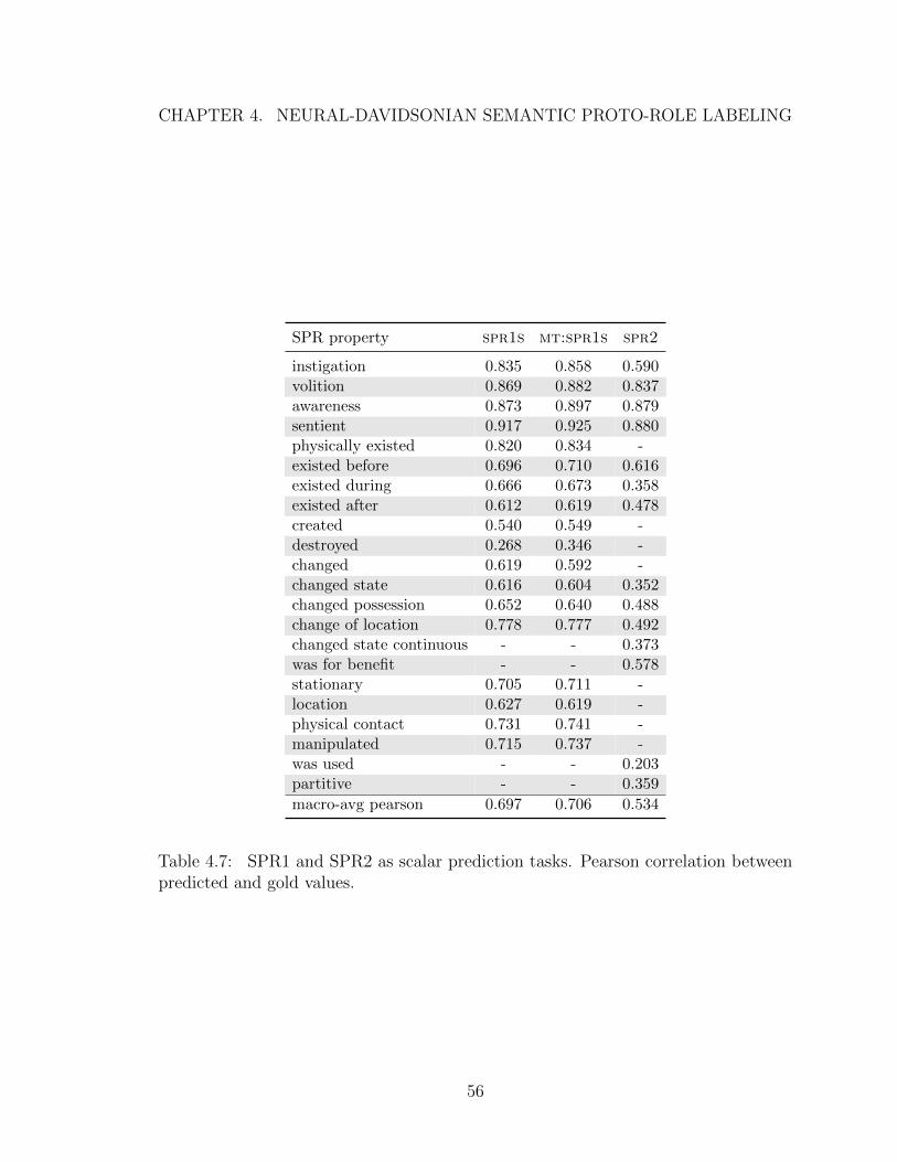
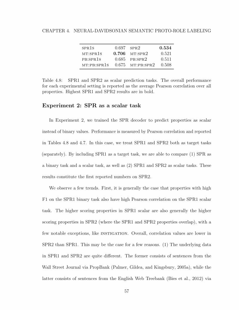
Table 4.8: SPR1 and SPR2 as scalar prediction tasks. The overall performancefor each experimental setting is reported as the average Pearson correlation over allproperties. Highest SPR1 and SPR2 results are in bold.

Experiment 2: SPR as a scalar task

In Experiment 2, we trained the SPR decoder to predict properties as scalar

instead of binary values. Performance is measured by Pearson correlation and reported

in Tables 4.8 and 4.7. In this case, we treat SPR1 and SPR2 both as target tasks

(separately). By including SPR1 as a target task, we are able to compare (1) SPR as

a binary task and a scalar task, as well as (2) SPR1 and SPR2 as scalar tasks. These

results constitute the first reported numbers on SPR2.

We observe a few trends. First, it is generally the case that properties with high

F1 on the SPR1 binary task also have high Pearson correlation on the SPR1 scalar

task. The higher scoring properties in SPR1 scalar are also generally the higher

scoring properties in SPR2 (where the SPR1 and SPR2 properties overlap), with a

few notable exceptions, like instigation. Overall, correlation values are lower in

SPR2 than SPR1. This may be the case for a few reasons. (1) The underlying data

in SPR1 and SPR2 are quite different. The former consists of sentences from the

Wall Street Journal via PropBank (Palmer, Gildea, and Kingsbury, 2005a), while the

latter consists of sentences from the English Web Treebank (Bies et al., 2012) via

57


the Universal Dependencies; (2) certain filters were applied in the construction of the

SPR1 dataset to remove instances where, e.g., predicates were embedded in a clause,

possibly resulting in an easier task; (3) SPR1 labels came from a single annotator

(after determining in pilot studies that annotations from this annotator correlated

well with other annotators), where SPR2 labels came from 24 different annotators

with scalar labels averaged over two-way redundancy.

Discussion

With SPR1 binary classification as the target task, we see overall improvements

from various multi-task training regimes (Experiments 1a-d, Tables 4.5 and 4.6), using

four different auxiliary tasks: machine translation into French, PropBank abstract role

prediction, word sense disambiguation (WordNet supersenses), and SPR2.19 These

auxiliary tasks exhibit a loose trade-off in terms of the quantity of available data

and the semantic relatedness of the task: MT is the least related task with the most

available (parallel) data, while SPR2 is the most related task with the smallest quantity

of data. While we hypothesized that the relatedness of PropBank role labeling and

word sense disambiguation tasks might lead to gains in SPR performance, we did not

see substantial gains in our experiments (pb:spr1, spr1+wsd). We did, however, see

improvements over the target-task only model (spr1) in the cases where we added

MT pretraining (mt:spr1) or SPR2 concurrent training (spr1+2). Interestingly,

19Note that in some cases we treat SPR2 as an auxiliary task, and in others, the target task.

58


combining MT pretraining with SPR2 concurrent training yielded no further gains

(mt:spr1+2).

4.7 Conclusion

Inspired by: (1) the SPR decomposition of predicate-argument relations into

overlapping feature bundles and (2) the neo-Davidsonian formalism for variable-arity

predicates, we have proposed a straightforward extension to a BiLSTM classification

framework in which the states of pre-identified predicate and argument tokens are

pairwise concatenated and used as the target for SPR prediction. We have shown that

our Neural-Davidsonian model outperforms the prior state of the art in aggregate and

showed especially large gains for properties of changed-possession, stationary,

and location. Our architecture naturally supports discrete or continuous label

paradigms, lends itself to multi-task initialization or concurrent training, and allows

for parameter sharing across properties. We demonstrated this sharing may be useful

when some properties are only sparsely annotated in the training data, which is

suggestive of future work in efficiently increasing the range of annotated SPR property

types.

59

Chapter 5

Event Factuality Prediction

A central function of natural language is to convey information about the properties

of events. Perhaps the most fundamental of these properties is factuality : whether

an event happened or not. In the context of Universal Decompositional Semantics

(UDS), we can conceive of factuality as an additional feature that characterizes an

event mentioned in text. Just as the proto-role properties introduced in Chapter 4

can be thought of as attributes of a participant in a particular event, factuality can

be thought of as a direct attribute of the event. As discussed in Chapter 3, event

factuality is a semantic attribute of events that we might like to convey in a Hobbsian

Logical Form event representation (e.g., with Hobbs’s Exist predicate on events), yet

this is information that cannot be directly read off of a sentence’s syntactic parse.

In this chapter, then, we are concerned with (1) the collection of semantic annota-

tions of factuality in natural language texts, and (2) the development of predictive

60

CHAPTER 5. EVENT FACTUALITY PREDICTION

factuality models as facilitated by the collection of this training data. Specifically,

we present two neural models for event factuality prediction, which yield significant

performance gains over previous models on three event factuality datasets: FactBank,

UW, and MEANTIME. We also present a substantial expansion of the It Happened

portion of the Universal Decompositional Semantics dataset (White et al., 2016a;

Rudinger, White, and Van Durme, 2018), yielding the largest event factuality dataset

to date.

5.1 Introduction

A natural language understanding system’s ability to accurately predict event

factuality is important for supporting downstream inferences that are based on those

events. For instance, if we aim to construct a knowledge base of events and their

participants, it is crucial that we know which events to include and which ones not to.

The event factuality prediction task (EFP) involves labeling event-denoting phrases

(or their heads) with the (non)factuality of the events denoted by those phrases (Saurı

and Pustejovsky, 2009; Saurı and Pustejovsky, 2012; Marneffe, Manning, and Potts,

2012). Figure 5.1 exemplifies such an annotation for the phrase headed by leave in

(1), which denotes a factual event (⊕=factual, ⊖=nonfactual).

(1) Jo failed to leave no trace. ⊕

61


Figure 5.1: Event factuality (⊕=factual) and inside v. outside context for leave inthe dependency tree.

In this chapter, we present two neural models of event factuality (and several variants

thereof). We show that these models significantly outperform previous systems on

four existing event factuality datasets – FactBank (Saurı and Pustejovsky, 2009), the

UW dataset (Lee et al., 2015), MEANTIME (Minard et al., 2016), and Universal

Decompositional Semantics It Happened v1 (UDS-IH1; White et al., 2016b) – and

we demonstrate the efficacy of multi-task training and ensembling in this setting.

In addition, we collect and release an extension of the UDS-IH1 dataset, which we

refer to as UDS-IH2, to cover the entirety of the English Universal Dependencies v1.2

(EUD1.2) treebank (Nivre et al., 2015), thereby yielding the largest event factuality

dataset to date.1

We begin with theoretical motivation for the models we propose as well as discussion

of prior EFP datasets and systems (Section 5.2). We then describe our own extension

of the UDS-IH1 dataset (Section 5.3), followed by our neural models (Section 5.4).

1Data available at decomp.io.

62

http://decomp.io


Using the data we collect, along with the existing datasets, we evaluate our models

(Section 5.6) in five experimental settings (Section 5.5) and analyze the results (Section

5.7).

5.2 Background

5.2.1 Linguistic description

Words from effectively every syntactic category can convey information about

the factuality of an event. For instance, negation (2-a), modal auxiliaries (2-b),

determiners (2-c), adverbs (2-d), verbs (2-e), adjectives (2-f), and nouns (2-g) can all

convey that a particular event – in the case of (2), a leaving event – did not happen.

(2) a. Jo didn’t leave.

b. Jo might leave.

c. Jo left no trace.

d. Jo never left.

e. Jo failed to leave.

f. Jo’s leaving was fake.

g. Jo’s leaving was a hallucination.

Further, such words can interact to yield non-trivial effects on factuality inferences:

63


(3-a) conveys that the leaving didn’t happen, while the superficially similar (3-b) does

not.

(3) a. Jo didn’t remember to leave. ⊖

b. Jo didn’t remember leaving. ⊕

A main goal of many theoretical treatments of factuality is to explain why these sorts

of interactions occur and how to predict them. While are there is a vast literature on

this problem, here we focus on the broad kinds of interactions our models need to be

able to capture in order to correctly predict the factuality of an event denoted by a

particular predicate—namely, interactions between that predicate’s outside and inside

context, exemplified in Figure 5.1.

Outside context

Factuality information coming from the outside context is well-studied in the do-

main of clause-embedding predicates, which break into at least four categories: factives,

like know and love (Kiparsky and Kiparsky, 1970; Karttunen, 1971b; Hintikka, 1975);

implicatives, like manage and fail (Karttunen, 1971a; Karttunen, 2012; Karttunen,

2013; Karttunen et al., 2014), veridicals, like prove and verify (Egr, 2008; Spector and

Egr, 2015), and non-veridicals, like hope and want.

Consider the factive-implicative verb forget (Karttunen, 1971a; White, 2014).

64


(4) a. Jo forgot that Bo left. ⊕

b. Jo forgot to leave. ⊖

(5) a. Jo didn’t forget that Bo left. ⊕

b. Jo didn’t forget to leave. ⊕

When a predicate directly embedded by forget is tensed, as in (4-a) and (5-a), we infer

that that predicate denotes a factual event, regardless of whether forget is negated.

In contrast, when a predicate directly embedded by forget is untensed, as in (4-b) and

(5-b), our inference is dependent on whether forget is negated. Thus, any model that

correctly predicts factuality will need to not only be able to represent the effect of

individual words in the outside context on factuality inferences, it will furthermore

need to represent their interaction.

Inside context

Knowledge of the inside context is important for integrating factuality information

coming from a predicate’s arguments—e.g. from determiners, like some and no.

(6) a. Some girl ate some dessert. ⊕

b. Some girl ate no dessert. ⊖

c. No girl ate no dessert. ⊕

In simple monoclausal sentences like those in (6), the number of arguments that

65


contain a negative quantifier, like no, determine the factuality of the event denoted

by the verb. An even number (or zero) will yield a factuality inference and an odd

number will yield a nonfactuality inference. Thus, as for outside context, any model

that correctly predicts factuality will need to integrate interactions between words in

the inside context.

The (non)necessity of syntactic information

One question that arises in the context of inside and outside information is whether

syntactic information is strictly necessary for capturing the relevant interactions be-

tween the two. To what extent is linear precedence sufficient for accurately computing

factuality?

We address these questions using two bidirectional LSTMs—one that has a linear

chain topology and another that has a dependency tree topology. Both networks

capture context on either side of an event-denoting word, but each does it in a different

way, depending on its topology. We show below that, while both networks outperform

previous models that rely on deterministic rules and/or hand-engineered features, the

linear chain-structured network reliably outperforms the tree-structured network.

5.2.2 Event factuality datasets

Saurı and Pustejovsky (2009) present the FactBank corpus of event factuality

annotations, built on top of the TimeBank corpus (Pustejovsky et al., 2006). These

66


annotations (performed by trained annotators) are discrete, consisting of an epistemic

modal {certain, probable, possible} and a polarity {+,−}. In FactBank, factuality

judgments are with respect to a source; following recent work, here we consider only

judgments with respect to a single source: the author. The smaller MEANTIME

corpus (Minard et al., 2016) includes similar discrete factuality annotations. Marneffe,

Manning, and Potts (2012) re-annotate a portion of FactBank using crowd-sourced

ordinal judgments to capture pragmatic effects on readers’ factuality judgments.

Lee et al. (2015) construct an event factuality dataset – henceforth, UW – on

the TempEval-3 data (UzZaman et al., 2013) using crowdsourced annotations on a

[−3, 3] scale (certainly did not happen to certainly did), with over 13,000 predicates.

Adopting the [−3, 3] scale of Lee et al. (2015), Stanovsky et al. (2017) assemble a

Unified Factuality dataset, mapping the discrete annotations of both FactBank and

MEANTIME onto the UW scale. Each scalar annotation corresponds to a token

representing the event, and each sentence may have more than one annotated token.

The UDS-IH1 dataset (White et al., 2016b) consists of factuality annotations over

6,920 event tokens, obtained with another crowdsourcing protocol. We adopt this

protocol, described in Section 5.3, to collect roughly triple this number of annotations.

We train and evaluate our factuality prediction models on this new dataset, UDS-IH2,

as well as the unified versions of UW, FactBank, and MEANTIME.

Table 5.1 shows the number of annotated predicates in each split of each factuality

dataset used in this paper. Annotations relevant to event factuality and polarity

67


Dataset Train Dev Test Total

FactBank 6636 2462 663 9761MEANTIME 967 210 218 1395UW 9422 3358 864 13644UDS-IH2 22108 2642 2539 27289

Table 5.1: Number of annotated predicates.

appear in a number of other resources, including the Penn Discourse Treebank (Prasad

et al., 2008), MPQA Opinion Corpus (Wiebe and Riloff, 2005), the LU corpus of

author belief commitments (Diab et al., 2009), and the ACE and ERE formalisms.

Soni et al. (2014) annotate Twitter data for factuality.

5.2.3 Event factuality systems

Nairn, Condoravdi, and Karttunen (2006) propose a deterministic algorithm based

on hand-engineered lexical features for determining event factuality. They associate

certain clause-embedding verbs with implication signatures (Table 5.2), which are used

in a recursive polarity propagation algorithm. TruthTeller is also a recursive rule-based

system for factuality (“predicate truth”) prediction using implication signatures, as

well as other lexical- and dependency tree-based features (Lotan, Stern, and Dagan,

2013).

Several systems use supervised models trained over rule-based features. Diab et al.

(2009) and Prabhakaran, Rambow, and Diab (2010) use SVMs and CRFs over lexical

and dependency features for predicting author belief commitments, which they treat as

68


a sequence tagging problem. Lee et al. (2015) train an SVM on lexical and dependency

path features for their factuality dataset. Saurı and Pustejovsky (2012) and Stanovsky

et al. (2017) train support vector models over the outputs of rule-based systems, the

latter with TruthTeller.

5.3 Data collection

Even the largest currently existing event factuality datasets are extremely small

from the perspective of related tasks, like natural language inference (NLI). Where

FactBank, UW, MEANTIME, and the original UDS-IH1 dataset have on the order of

30,000 labeled examples combined, standard NLI datasets, like the Stanford Natural

Language Inference (SNLI; (Bowman, Potts, and Manning 2015a)) dataset, have on

the order of 500,000.

To begin to remedy this situation, we collect an extension of the UDS-IH1 dataset.

The resulting UDS-IH2 dataset covers all predicates in EUD1.2. Beyond substantially

expanding the amount of publicly available event factuality annotations, another

major benefit is that EUD1.2 consists entirely of gold parses and has a variety of other

annotations built on top of it, making future multi-task modeling possible.

We use the protocol described by White et al. (2016b) to construct UDS-IH2. This

protocol involves four kinds of questions for a particular predicate candidate:

1. understandable: whether the sentence is understandable

69


2. predicate: whether or not a particular word refers to an eventuality (event or

state)

3. happened: whether or not, according to the author, the event has already

happened or is currently happening

4. confidence: how confident the annotator is about their answer to happened

from 0-4

If an annotator answers no to either understandable or predicate, happened

and confidence do not appear.

The main differences between this protocol and the others discussed above are: (i)

instead of asking about annotator confidence, the other protocols ask the annotator

to judge either source confidence or likelihood; and (ii) factuality and confidence are

separated into two questions. We choose to retain White et al.’s protocol to maintain

consistency with the portions of EUD1.2 that were already annotated in UDS-IH1.

Annotators

We recruited 32 unique annotators through Amazon’s Mechanical Turk to annotate

20,580 total predicates in groups of 10. Each predicate was annotated by two distinct

annotators. Including UDS-IH1, this brings the total number of annotated predicates

to 27,289.

Raw inter-annotator agreement for the happened question was 0.84 (Cohen’s

κ=0.66) among the predicates annotated only for UDS-IH2. This compares to the

70


●●●

●

●●●

●

●●●●

●

●●●

●●●●

●

●

●

●●

●

●

●

●

●

●

●

−3 −2 −1 0 1 2 3

●

●

●

●

FactBankUWMEANTIMEUDS−IH2

Figure 5.2: Relative frequency of factuality ratings in training and development sets.

raw agreement score of 0.82 reported by White et al. (2016b) for UDS-IH1.

To improve the overall quality of the annotations, we filter annotations from

annotators that display particularly low agreement with other annotators on happened

and confidence.

Pre-processing

To compare model results on UDS-IH2 to those found in the unified datasets of

Stanovsky et al. (2017), we map the happened and confidence ratings to a single

factuality value in [-3,3] by first taking the mean confidence rating for each predi-

cate and mapping factuality to 34confidence if happened and -3

4confidence

otherwise.

71


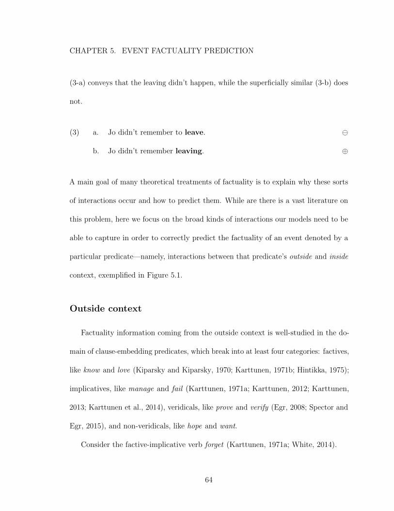
Response distribution

Figure 5.2 plots the distribution of factuality ratings in the train and dev splits for

UDS-IH2, alongside those of FactBank, UW, and MEANTIME. One striking feature

of these distributions is that UDS-IH2 displays a much more entropic distribution

than the other datasets. This may be due to the fact that, unlike the newswire-heavy

corpora that the other datasets annotate, EUD1.2 contains text from genres – weblogs,

newsgroups, email, reviews, and question-answers – that tend to involve less reporting

of raw facts. One consequence of this more entropic distribution is that, unlike the

datasets discussed above, it is much harder for systems that always guess 3 – i.e.

factual with high confidence/likelihood – to perform well.

5.4 Models

We consider two neural models of factuality: a stacked bidirectional linear chain

LSTM (§5.4.1) and a stacked bidirectional child-sum dependency tree LSTM (§5.4.2).

To predict the factuality vt for the event referred to by a word wt, we use the hidden

state at t from the final layer of the stack as the input to a two-layer regression model

(§5.4.3).

72


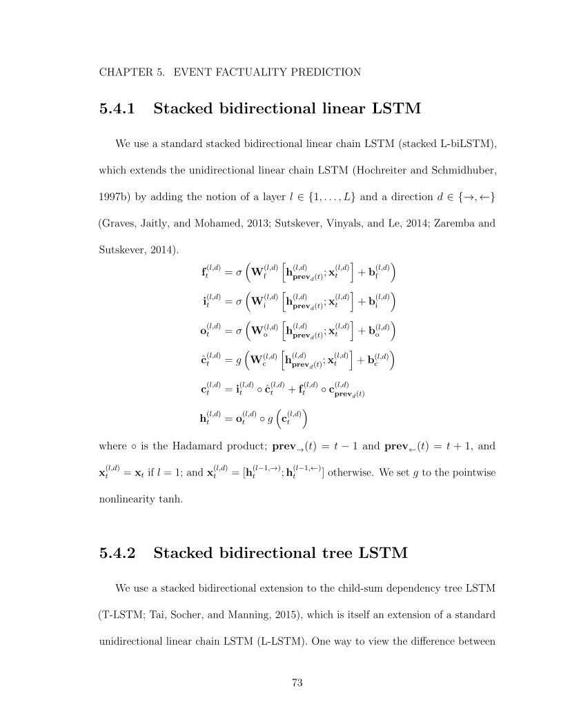
5.4.1 Stacked bidirectional linear LSTM

We use a standard stacked bidirectional linear chain LSTM (stacked L-biLSTM),

which extends the unidirectional linear chain LSTM (Hochreiter and Schmidhuber,

1997b) by adding the notion of a layer l ∈ {1, . . . , L} and a direction d ∈ {→,←}

(Graves, Jaitly, and Mohamed, 2013; Sutskever, Vinyals, and Le, 2014; Zaremba and

Sutskever, 2014).

f(l,d)t = σ

(W

(l,d)f

[h(l,d)prevd(t)

;x(l,d)t

]+ b

(l,d)f

)i(l,d)t = σ

(W

(l,d)i

[h(l,d)prevd(t)

;x(l,d)t

]+ b

(l,d)i

)o(l,d)t = σ

(W(l,d)

o

[h(l,d)prevd(t)

;x(l,d)t

]+ b(l,d)

o

)c(l,d)t = g

(W(l,d)

c

[h(l,d)prevd(t)

;x(l,d)t

]+ b(l,d)

c

)c(l,d)t = i

(l,d)t ◦ c(l,d)t + f

(l,d)t ◦ c(l,d)prevd(t)

h(l,d)t = o

(l,d)t ◦ g

(c(l,d)t

)where ◦ is the Hadamard product; prev→(t) = t − 1 and prev←(t) = t + 1, and

x(l,d)t = xt if l = 1; and x

(l,d)t = [h

(l−1,→)t ;h

(l−1,←)t ] otherwise. We set g to the pointwise

nonlinearity tanh.

5.4.2 Stacked bidirectional tree LSTM

We use a stacked bidirectional extension to the child-sum dependency tree LSTM

(T-LSTM; Tai, Socher, and Manning, 2015), which is itself an extension of a standard

unidirectional linear chain LSTM (L-LSTM). One way to view the difference between

73


the L-LSTM and the T-LSTM is that the T-LSTM redefines prev→(t) to return the

set of indices that correspond to the children of wt in some dependency tree. Because

the cardinality of these sets varies with t, it is necessary to specify how multiple

children are combined. The basic idea, which we make explicit in the equations for

our extension, is to define ftk for each child index k ∈ prev→(t) in a way analogous to

the equations in §5.4.1 – i.e. as though each child were the only child – and then sum

across k within the equations for it, ot, ct, ct, and ht.

Our stacked bidirectional extension (stacked T-biLSTM) is a minimal extension to

the T-LSTM in the sense that we merely define the downward computation in terms

of a prev←(t) that returns the set of indices that correspond to the parents of wt in

some dependency tree (cf. (Miwa and Bansal 2016), who propose a similar, but less

minimal, model for relation extraction). The same method for combining children in

the upward computation can then be used for combining parents in the downward

computation. This yields a minimal change to the stacked L-biLSTM equations.

74


f(l,d)tk = σ

(W

(l,d)f

[h(l,d)k ;x

(l,d)t

]+ b

(l,d)f

)h(l,d)t =

∑k∈prevd(t)

h(l,d)k

i(l,d)t = σ

(W

(l,d)i

[h(l,d)t ;x

(l,d)t

]+ b

(l,d)i

)o(l,d)t = σ

(W(l,d)

o

[h(l,d)t ;x

(l,d)t

]+ b(l,d)

o

)c(l,d)t = g

(W(l,d)

c

[h(l,d)t ;x

(l,d)t

]+ b(l,d)

c

)c(l,d)t = i

(l,d)t ◦ c(l,d)t +

∑k∈prevd(t)

f(l,d)tk ◦ c(l,d)k

h(l,d)t = o

(l,d)t ◦ g

(c(l,d)t

)We use a ReLU pointwise nonlinearity for g. These minimal changes allow us to

represent the inside and the outside contexts of word t (at layer l) as single vectors:

h(l,→)t and h

(l,←)t .

An important thing to note here is that – in contrast to other dependency tree-

structured T-LSTMs (Socher et al., 2014; Iyyer et al., 2014) – this T-biLSTM definition

does not use the dependency labels in any way. Such labels could be straightforwardly

incorporated to determine which parameters are used in a particular cell, but for

current purposes, we retain the simpler structure (i) to more directly compare the L-

and T-biLSTMs and (ii) because a model that uses dependency labels substantially

increases the number of trainable parameters, relative to the size of our datasets.

75


5.4.3 Regression model

To predict the factuality vt for the event referred to by a word wt, we use the

hidden states from the final layer of the stacked L- or T-biLSTM as the input to a

two-layer regression model.

h(L)t = [h

(L,→)t ;h

(L,←)t ]

vt = V2 g(V1h

(L)t + b1

)+ b2

where vt is passed to a loss function L(vt, vt): in this case, smooth L1 – i.e. Huber

loss with δ = 1. This loss function is effectively a smooth variant of the hinge loss

used by Lee et al. (2015) and Stanovsky et al. (2017).

We also consider a simple ensemble method, wherein the hidden states from the

final layers of both the stacked L-biLSTM and the stacked T-biLSTM are concatenated

and passed through the same two-layer regression model. We refer to this as the

H(ybrid)-biLSTM.2

2See Miwa and Bansal (2016) and Bowman et al. (2016) for alternative ways of hybridizing linearand tree LSTMs for semantic tasks. We use the current method since it allows us to make minimalchanges to the architectures of each model, which in turn allows us to assess the two models’ abilityto capture different aspects of factuality.

76


5.5 Experiments

Implementation

We implement both the L-biLSTM and T-biLSTM models using pytorch 0.2.0.

The L-biLSTM model uses the stock implementation of the stacked bidirectional

linear chain LSTM found in pytorch, and the T-biLSTM model uses a custom

implementation, which we make available at decomp.net.

Word embeddings

We use the 300-dimensional GloVe 42B uncased word embeddings (Pennington,

Socher, and Manning, 2014) with an UNK embedding whose dimensions are sampled

iid from a Uniform[-1,1]. We do not tune these embeddings during training.

Hidden state sizes

We set the dimension of the hidden states h(l,d)t and cell states c

(l,d)t to 300 for all

layers of the stacked L- and stacked T-biLSTMs – the same size as the input word

embeddings. This means that the input to the regression model is 600-dimensional,

for the stacked L- and T-biLSTMs, and 1200-dimensional, for the stacked H-biLSTM.

For the hidden layer of the regression component, we set the dimension to half the

size of the input hidden state: 300, for the stacked L- and T-biLSTMs, and 600, for

the stacked H-biLSTM.

77

http://decomp.net


Bidirectional layers

We consider stacked L-, T-, and H-biLSTMs with either one or two layers. In

preliminary experiments, we found that networks with three layers badly overfit the

training data.

Dependency parses

For the T- and H-biLSTMs, we use the gold dependency parses provided in EUD1.2

when training and testing on UDS-IH2. On FactBank, MEANTIME, and UW, we

follow Stanovsky et al. (2017) in using the automatic dependency parses generated by

the parser in spaCy (Honnibal and Johnson, 2015).3

Lexical features

Recent work on neural models in the closely related domain of genericity/habituality

prediction suggests that inclusion of hand-annotated lexical features can improve

classification performance (Becker et al., 2017). To assess whether similar performance

gains can be obtained here, we experiment with lexical features for simple factive and

implicative verbs (Kiparsky and Kiparsky, 1970; Karttunen, 1971a). When in use,

these features are concatenated to the network’s input word embeddings so that, in

principle, they may interact with one another and inform other hidden states in the

biLSTM, akin to how verbal implicatives and factives are observed to influence the

3In rebuilding the Unified Factuality dataset (Stanovsky et al., 2017), we found that sentencesplitting was potentially sensitive to the version of spaCy used. We used v1.9.0.

78


Verb Signature Type Example

know +|+ fact. Jo knew that Bo ate.manage +|− impl. Jo managed to go.neglect −|+ impl. Jo neglected to call Bo.hesitate ◦|+ impl. Jo didn’t hesitate to go.attempt ◦|− impl. Jo didn’t attempt to go.

Table 5.2: Implication signature features from Nairn, Condoravdi, and Karttunen(2006). As an example, a signature of −|+ indicates negative implication underpositive polarity (left side) and positive implication under negative polarity (rightside); ◦ indicates neither positive nor negative implication.

factuality of their complements. The hidden state size is increased to match the input

embedding size. We consider two types:

Signature features We compute binary features based on a curated list of 92

simple implicative and 95 factive verbs including their their type-level “implication

signatures,” as compiled by Nairn, Condoravdi, and Karttunen (2006).4 These

signatures characterize the implicative or factive behavior of a verb with respect to its

complement clause, how this behavior changes (or does not change) under negation,

and how it composes with other such verbs under nested recursion. We create one

indicator feature for each signature type. Examples of these signature features are

presented in Table 5.2.

Mined features Using a simplified set of pattern matching rules over Common

Crawl data (Buck, Heafield, and Ooyen, 2014), we follow the insights of Pavlick and

Callison-Burch (2016) – henceforth, PC – and use corpus mining to automatically score

verbs for implicativeness. The insight of PC lies in Karttunen’s (1971) observation

4http://web.stanford.edu/group/csli_lnr/Lexical_Resources

79

http://web.stanford.edu/group/csli_lnr/Lexical_Resources


dare to 1.00 intend to 0.83bother to 1.00 want to 0.77happen to 0.99 decide to 0.75forget to 0.99 promise to 0.75manage to 0.97 agree to 0.35try to 0.96 plan to 0.20get to 0.90 hope to 0.05venture to 0.85

Table 5.3: Implicative (bold) and non-implicative (not bold) verbs from Karttunen(1971a) are nearly separable by our tense agreement scores, replicating the results ofPC.

that “the main sentence containing an implicative predicate and the complement

sentence necessarily agree in tense.”

Accordingly, PC devise a tense agreement score – effectively, the ratio of times an

embedding predicate’s tense matches the tense of the predicate it embeds – to predict

implicativeness in English verbs. Their scoring method involves the use of fine-grained

POS tags, the Stanford Temporal Tagger (Chang and Manning, 2012), and a number

of heuristic rules, which resulted in a confirmation that tense agreement statistics are

predictive of implicativeness, illustrated in part by observing a near perfect separation

of a list of implicative and non-implicative verbs from Karttunen (1971a).

We replicate this finding by employing a simplified pattern matching method

over 3B sentences of raw Common Crawl text. We efficiently search for instances

of any pattern of the form: I $VERB to * $TIME, where $VERB and $TIME are pre-

instantiated variables so their corresponding tenses are known, and ‘*’ matches any one

to three whitespace-separated tokens at runtime (not pre-instantiated). To instantiate

$VERB, we use a list of 1K clause-embedding verbs compiled by (White and Rawlins,

80


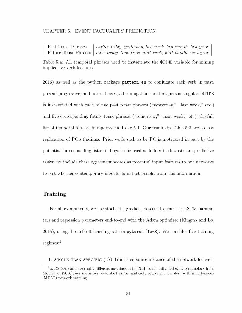
Past Tense Phrases earlier today, yesterday, last week, last month, last yearFuture Tense Phrases later today, tomorrow, next week, next month, next year

Table 5.4: All temporal phrases used to instantiate the $TIME variable for miningimplicative verb features.

2016) as well as the python package pattern-en to conjugate each verb in past,

present progressive, and future tenses; all conjugations are first-person singular. $TIME

is instantiated with each of five past tense phrases (“yesterday,” “last week,” etc.)

and five corresponding future tense phrases (“tomorrow,” “next week,” etc); the full

list of temporal phrases is reported in Table 5.4. Our results in Table 5.3 are a close

replication of PC’s findings. Prior work such as by PC is motivated in part by the

potential for corpus-linguistic findings to be used as fodder in downstream predictive

tasks: we include these agreement scores as potential input features to our networks

to test whether contemporary models do in fact benefit from this information.

Training

For all experiments, we use stochastic gradient descent to train the LSTM parame-

ters and regression parameters end-to-end with the Adam optimizer (Kingma and Ba,

2015), using the default learning rate in pytorch (1e-3). We consider five training

regimes:5

1. single-task specific (-S) Train a separate instance of the network for each

5Multi-task can have subtly different meanings in the NLP community; following terminology fromMou et al. (2016), our use is best described as “semantically equivalent transfer” with simultaneous(MULT) network training.

81


dataset, training only on that dataset.

2. single-task general (-G) Train one instance of the network on the simple

concatenation of all unified factuality datasets, {FactBank, UW, MEANTIME}.

3. multi-task simple (-MultiSimp) Same as single-task general, except

the network maintains a distinct set of regression parameters for each dataset;

all other parameters (LSTM) remain tied. “w/UDS-IH2” is specified if UDS-IH2

is included in training.

4. multi-task balanced (-MultiBal) Same as multi-task simple but up-

sampling examples from the smaller datasets to ensure that examples from those

datasets are seen at the same rate.

5. multi-task focused (-MultiFoc) Same as multi-task simple but upsam-

pling examples from a particular target dataset to ensure that examples from

that dataset are seen 50% of the time and examples from the other datasets are

seen 50% (evenly distributed across the other datasets).

Calibration

Post-training, network predictions are monotonically re-adjusted to a specific

dataset using isotonic regression (fit on train split only).

82


Evaluation

Following Lee et al. (2015) and Stanovsky et al. (2017), we report two evaluation

measures: mean absolute error (MAE) and Pearson correlation (r). We would like

to note, however, that we believe correlation to be a better indicator of performance

for two reasons: (i) for datasets with a high degree of label imbalance (Figure 5.2), a

baseline that always guesses the mean or mode label can be difficult to beat in terms

of MAE but not correlation, and (ii) MAE is harder to meaningfully compare across

datasets with different label mean and variance.

Development

Under all regimes, we train the model for 20 epochs – by which time all models

appear to converge. We save the parameter values after the completion of each epoch

and then score each set of saved parameter values on the development set for each

dataset. The set of parameter values that performed best on the development set in

terms of Pearson correlation for a particular dataset were then used to score the test

set for that dataset.

83


5.6 Results

Table 5.5 reports the results for all of the 2-layer L-, T-, and H-biLSTMs.6 The

best-performing system for each dataset and metric are highlighted in purple, and

when the best-performing system for a particular dataset was a 1-layer model, that

system is included in Table 5.5. The full set of results for all 1-layer and 2-layer models

for both development and test splits can be found in Table 5.11 at the end of this

chapter.

New state of the art

For each dataset and metric, with the exception of MAE on UW, we achieve state

of the art results with multiple systems. The highest-performing system for each is

reported in Table 5.5. Our results on UDS-IH2 are the first reported numbers for this

new factuality resource.

Linear v. tree topology

On its own, the biLSTM with linear topology (L-biLSTM) performs consistently

better than the biLSTM with tree topology (T-biLSTM). However, the hybrid topology

(H-biLSTM), consisting of both a L- and T-biLSTM is the top-performing system on

UW for correlation (Table 5.5). This suggests that the T-biLSTM may be contributing

6Full results are reported in Table 5.11. Note that the 2-layer networks do not strictly dominatethe 1-layer networks in terms of MAE and correlation.

84


FactB

ank

UW

Meantime

UDS-IH2

MAE

rMAE

rMAE

rMAE

r

All-3.0

0.8

NAN

0.78

NAN

0.31

NAN

2.25

5NAN

Lee

etal.20

15

--

0.51

10.70

8-

--

-Stanovskyet

al.20

17

0.59

0.71

0.42†

0.66

0.34

0.47

--

L-biLSTM(2)-S

0.427

0.826

0.50

80.719

0.42

70.33

50.960†

0.768

T-biLSTM(2)-S

0.577

0.752

0.60

00.64

50.42

80.09

41.101

0.704

L-biLSTM(2)-G

0.412

0.812

0.52

30.70

30.40

90.46

2-

-T-biLSTM(2)-G

0.455

0.809

0.56

70.68

80.39

60.36

8-

-

L-biLSTM(2)-S+lexfeats

0.429

0.796

0.49

50.730

0.42

70.32

21.000

0.755

T-biLSTM(2)-S+lexfeats

0.542

0.744

0.56

70.67

60.37

50.24

21.087

0.719

L-biLSTM(2)-MultiSim

p0.353

0.843

0.50

30.725

0.34

50.540

--

T-biLSTM(2)-MultiSim

p0.482

0.803

0.59

90.64

50.54

50.23

7-

-L-biLSTM(2)-MultiBal

0.391

0.821

0.49

60.724

0.278

0.613†

--

T-biLSTM(2)-MultiBal

0.517

0.788

0.57

30.65

90.40

00.40

5-

-L-biLSTM(1)-MultiFoc

0.343

0.823

0.51

60.69

80.229†

0.599

--

L-biLSTM(2)-MultiFoc

0.314

0.846

0.50

20.710

0.305

0.37

7-

-T-biLSTM(2)-MultiFoc

1.10

00.23

40.61

50.61

60.39

50.30

0-

-L-biLSTM(2)-MultiSim

pw/U

DS-IH2

0.377

0.828

0.50

80.722

0.36

70.46

90.965

0.771†

T-biLSTM(2)-MultiSim

pw/UDS-IH2

0.59

50.716

0.59

80.60

90.46

70.34

51.072

0.723

H-biLSTM(2)-S

0.48

80.775

0.52

60.714

0.44

20.25

50.967

0.768

H-biLSTM(1)-MultiSim

p0.313†

0.857†

0.52

80.70

40.31

40.54

5-

-H-biLSTM(2)-MultiSim

p0.431

0.808

0.51

40.723

0.40

10.46

1-

-H-biLSTM(2)-MultiBal

0.386

0.825

0.50

20.713

0.35

20.564

--

H-biLSTM(2)-MultiSim

pw/U

DS-IH2

0.393

0.820

0.48

10.749†

0.37

40.495

0.969

0.760

Tab

le5.

5:A

ll2-

laye

rsy

stem

s,an

d1-

laye

rsy

stem

sif

bes

tin

colu

mn

.S

tate

-of-

the-

art

inb

old

;†

isb

est

inco

lum

n(w

ith

row

shad

edin

pu

rple

).K

ey:

L=

lin

ear,

T=

tree

,H

=hyb

rid

,(1

,2)=

#la

yers

,S

=si

ngl

e-ta

sksp

ecifi

c,G

=si

ngl

e-ta

skge

ner

al,

+le

xfe

ats=

wit

hal

lle

xic

alfe

atu

res,

Mu

ltiS

imp

=m

ult

i-ta

sksi

mp

le,

Mu

ltiB

al=

mu

lti-

task

bal

ance

d,

Mu

ltiF

oc=

mu

lti-

task

focu

sed

,w

/UD

S-I

H2=

trai

ned

onal

ld

ata

incl

.U

DS

-IH

2.A

ll-3

.0is

the

con

stan

tb

asel

ine.

85


MeanRelation Label L-biLSTM T-biLSTM #

root 1.07 1.03 0.96 949conj 0.37 0.44 0.46 316advcl 0.46 0.53 0.45 303xcomp -0.42 -0.57 -0.49 234acl:relcl 1.28 1.40 1.31 193ccomp 0.11 0.31 0.34 191acl 0.77 0.59 0.58 159parataxis 0.44 0.63 0.79 127amod 1.92 1.88 1.81 76csubj 0.36 0.38 0.27 37

Table 5.6: Mean predictions for linear (L-biLSTM-S(2)) and tree models (T-biLSTM-S(2)) on UDS-IH2-dev, grouped by governing dependency relation. Only the 10 mostfrequent governing dependency relations in UDS-IH2-dev are shown.

something complementary to the L-biLSTM.

Evidence of this complementarity can be seen in Table 5.6, which contains a

breakdown of system performance by governing dependency relation, for both linear

and tree models, on UDS-IH2-dev. In most cases, the L-biLSTM’s mean prediction is

closer to the true mean. This appears to arise in part because the T-biLSTM is less

confident in its predictions – i.e. its mean prediction tends to be closer to 0. This

results in the L-biLSTM being too confident in certain cases – e.g. in the case of the

xcomp governing relation, where the T-biLSTM mean prediction is closer to the true

mean.

86


Lexical features have minimal impact

Adding all lexical features (both signature and mined) yields mixed results.

We see slight improvements on UW, while performance on the other datasets mostly

declines (compare with single-task specific). Factuality prediction is precisely

the kind of NLP task one would expect these types of features to assist with, so it is

notable that, in our experiments, they do not.

Multi-task helps

Though our methods achieve state of the art in the single-task setting, the best

performing systems are mostly multi-task (Table 5.5 and 5.11). This is an ideal

setting for multi-task training: each dataset is relatively small, and their labels capture

closely-related (if not identical) linguistic phenomena. UDS-IH2, the largest by a

factor of two, reaps the smallest gains from multi-task.

5.7 Analysis

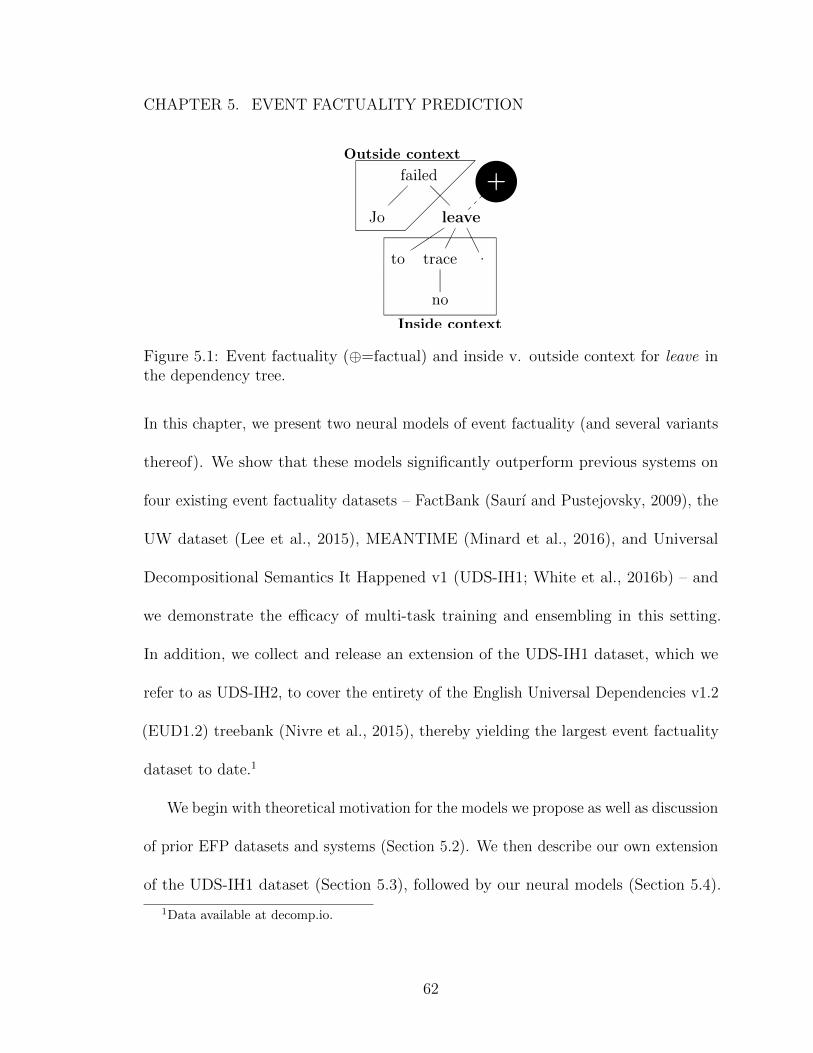
As discussed in Section 5.2, many discrete linguistic phenomena interact with event

factuality. Here we provide a brief analysis of some of those interactions, both as

they manifest in the UDS-IH2 dataset, as well as in the behavior of our models. This

analysis employs the gold dependency parses present in EUD1.2.

Table 5.7 illustrates the influence of modals and negation on the factuality of the

87


Mean Linear TreeModal Negated Label MAE MAE #

none no 1.00 0.93 1.03 2244none yes -0.19 1.40 1.69 98may no -0.38 1.00 0.99 14would no -0.61 0.85 0.99 39ca(n’t) yes -0.72 1.28 1.55 11can yes -0.75 0.99 0.86 6(wi)’ll no -0.94 1.47 1.14 8could no -1.03 0.97 1.32 20can no -1.25 1.02 1.21 73might no -1.25 0.66 1.06 6would yes -1.27 0.40 0.86 5should no -1.31 1.20 1.01 22will no -1.88 0.75 0.86 75

Table 5.7: Mean gold labels, counts, and MAE for L-biLSTM(2)-S and T-biLSTM(2)-Smodel predictions on UDS-IH2-dev, grouped by modals and negation.

events they have direct scope over. The context with the highest factuality on average

is no direct modal and no negation (first row); all other modal contexts have varying

degrees of negative mean factuality scores, with will as the most negative. This is

likely a result of UDS-IH2 annotation instructions to mark future events as not having

happened.

Table 5.8 shows results from a manual error analysis on 50 events from UDS-IH2-

dev with highest absolute prediction error (using H-biLSTM(2)-MultiSim w/UDS-

IH2). Grammatical errors (such as run-on sentences) in the underlying text of UDS-

IH2 appear to pose a particular challenge for these models; informal language and

grammatical errors in UDS-IH2 is a substantial distinction from the other factuality

datasets used here.

In Section 5.6 we observe that the linguistically-motivated lexical features that we

88


Attribute #

Grammatical error present, incl. run-ons 16Is an auxiliary or light verb 14Annotation is incorrect 13Future event 12Is a question 5Is an imperative 3Is not an event or state 2

One or more of the above 43

Table 5.8: Notable attributes of 50 instances from UDS-IH2-dev with highest absoluteprediction error (using H-biLSTM(2)-MultiSim w/UDS-IH2).

manage to 2.78 agree to -1.00happen to 2.34 forget to -1.18dare to 1.50 want to -1.48bother to 1.50 intend to -2.02decide to 0.10 promise to -2.34get to -0.23 plan to -2.42try to -0.24 hope to -2.49

Table 5.9: UDS-IH2-train: Infinitival-taking verbs sorted by the mean annotationscores of their complements (xcomp), with direct negation filtered out. Implicativesare in bold.

test (+lexfeats) do not have a big impact on overall performance. Tables 5.9 and 5.10

help nuance this observation.

Table 5.9 shows that we can achieve similar separation between implicatives and

non-implicatives as the feature mining strategy presented in Section 5.5. That is,

those features may be redundant with information already learnable from factuality

datasets (UDS-IH2). Despite the underperformance of these features overall, Table

5.10 shows that they may still improve performance in the subset of instances where

they appear.

89


Verb L-biLSTM(2)-S +lexfeats #

decide to 3.28 2.66 2forget to 0.67 0.48 2get to 1.55 1.43 9hope to 1.35 1.23 5intend to 1.18 0.61 1promise to 0.40 0.49 1try to 1.14 1.42 12want to 1.22 1.17 24

Table 5.10: MAE of L-biLSTM(2)-S and L-biLSTM(2)-S+lexfeats, for predictions onevents in UDS-IH2-dev that are xcomp-governed by an infinitival-taking verb.

5.8 Conclusion

We have proposed two neural models of event factuality prediction – a bidirectional

linear-chain LSTM (L-biLSTM) and a bidirectional child-sum dependency tree LSTM

(T-biLSTM) – which yield substantial gains over previous models based on deterministic

rules and hand-engineered features. We found that both models yield such gains,

though the L-biLSTM outperforms the T-biLSTM; for some datasets, an ensemble of

the two (H-biLSTM) improves over either alone.

We have also extended the UDS-IH1 dataset, yielding the largest publicly-available

factuality dataset to date: UDS-IH2. In experiments, we see substantial gains from

multi-task training over the three factuality datasets unified by Stanovsky et al. (2017),

as well as UDS-IH2. Future work will further probe the behavior of these models, or

extend them to learn other aspects of event semantics.

90


FactB

ank

UW

Meantime

UD

dev

test

dev

test

dev

test

dev

test

MAE

rM

AE

rM

AE

rM

AE

rM

AE

rM

AE

rM

AE

rM

AE

r

All-3

.0-

-0.8

0-

-0.78

0-

-0.31

0-

-2.255

0Leeetal.

2015

--

--

0.462

0.749

0.511

0.708

--

--

--

--

Sta

novsk

yetal.

2017

--

0.59

0.71

--

0.42

0.66

--

0.31

0.47

--

--

L-b

iLSTM

(1)-S

0.411

0.78

0.399

0.816

0.435

0.797

0.508

0.718

0.239

0.631

0.337

0.359

0.978

0.768

0.986

0.765

L-b

iLSTM

(2)-S

0.482

0.772

0.427

0.826

0.426

0.799

0.508

0.719

0.357

0.601

0.427

0.335

0.95

0.771

0.96

0.768

T-b

iLSTM

(1)-S

0.564

0.711

0.48

0.748

0.491

0.734

0.574

0.652

0.297

0.564

0.36

0.155

1.043

0.739

1.053

0.725

T-b

iLSTM

(2)-S

0.595

0.71

0.577

0.752

0.497

0.735

0.6

0.645

0.351

0.371

0.428

0.094

1.06

0.719

1.101

0.704

L-b

iLSTM

(1)-G

0.432

0.798

0.383

0.819

0.426

0.807

0.517

0.717

0.252

0.625

0.343

0.505

--

--

L-b

iLSTM

(2)-G

0.439

0.799

0.412

0.812

0.42

0.809

0.523

0.703

0.291

0.604

0.409

0.462

--

--

T-b

iLSTM

(1)-G

0.468

0.758

0.405

0.82

0.472

0.76

0.571

0.662

0.336

0.509

0.408

0.384

--

--

T-b

iLSTM

(2)-G

0.498

0.764

0.455

0.809

0.481

0.757

0.567

0.688

0.298

0.527

0.396

0.368

--

--

L-b

iLSTM

(1)-S+lexfeats:sign

0.423

0.78

0.396

0.805

--

--

--

--

--

--

L-b

iLSTM

(2)-S+lexfeats:sign

0.459

0.768

0.423

0.82

--

--

--

--

--

--

T-b

iLSTM

(1)-S+lexfeats:sign

0.54

0.718

0.51

0.762

--

--

--

--

--

--

T-b

iLSTM

(2)-S+lexfeats:sign

0.552

0.731

0.558

0.748

--

--

--

--

--

--

L-b

iLSTM

(1)-S+lexfeats:m

ine

0.468

0.781

0.453

0.801

--

--

--

--

--

--

L-b

iLSTM

(2)-S+lexfeats:m

ine

0.416

0.768

0.373

0.808

--

--

--

--

--

--

T-b

iLSTM

(1)-S+lexfeats:m

ine

0.546

0.725

0.525

0.751

--

--

--

--

--

--

T-b

iLSTM

(2)-S+lexfeats:m

ine

0.567

0.727

0.573

0.72

--

--

--

--

--

--

L-b

iLSTM

(1)-S+lexfeats:b

oth

0.443

0.781

0.413

0.805

0.428

0.803

0.507

0.722

0.319

0.481

0.373

0.369

1.002

0.762

1.002

0.766

L-b

iLSTM

(2)-S+lexfeats:b

oth

0.485

0.764

0.429

0.796

0.433

0.792

0.495

0.73

0.356

0.662

0.427

0.322

0.977

0.767

10.755

T-b

iLSTM

(1)-S+lexfeats:b

oth

0.503

0.728

0.449

0.793

0.485

0.743

0.589

0.643

0.282

0.493

0.348

0.191

1.04

0.738

1.073

0.718

T-b

iLSTM

(2)-S+lexfeats:b

oth

0.565

0.724

0.542

0.744

0.481

0.747

0.567

0.676

0.352

0.404

0.375

0.242

1.049

0.738

1.087

0.719

L-b

iLSTM

(1)-M

ultiS

imp

0.408

0.804

0.365

0.834

0.414

0.825

0.506

0.736

0.241

0.506

0.286

0.453

--

--

L-b

iLSTM

(2)-M

ultiS

imp

0.393

0.811

0.353

0.843

0.417

0.817

0.503

0.725

0.314

0.56

0.345

0.54

--

--

T-b

iLSTM

(1)-M

ultiS

imp

0.464

0.756

0.408

0.807

0.472

0.754

0.555

0.67

0.248

0.546

0.318

0.357

--

--

T-b

iLSTM

(2)-M

ultiS

imp

0.517

0.753

0.482

0.803

0.493

0.754

0.599

0.645

0.474

0.52

0.545

0.237

--

--

L-b

iLSTM

(1)-M

ultiB

al

0.387

0.805

0.332

0.841

0.412

0.822

0.52

0.722

0.232

0.57

0.256

0.544

--

--

L-b

iLSTM

(2)-M

ultiB

al

0.441

0.8

0.391

0.821

0.414

0.815

0.496

0.724

0.251

0.624

0.278

0.613

--

--

T-b

iLSTM

(1)-M

ultiB

al

0.475

0.746

0.405

0.817

0.472

0.752

0.578

0.629

0.237

0.56

0.344

0.266

--

--

T-b

iLSTM

(2)-M

ultiB

al

0.56

0.73

0.517

0.788

0.499

0.734

0.573

0.659

0.252

0.567

0.4

0.405

--

--

L-b

iLSTM

(1)-M

ultiF

oc

0.378

0.79

0.343

0.823

0.414

0.813

0.516

0.698

0.256

0.48

0.229

0.599

--

--

L-b

iLSTM

(2)-M

ultiF

oc

0.379

0.808

0.314

0.846

0.409

0.81

0.502

0.71

0.227

0.524

0.305

0.377

--

--

T-b

iLSTM

(1)-M

ultiF

oc

0.469

0.748

0.401

0.81

0.474

0.754

0.579

0.654

0.29

0.533

0.354

0.293

--

--

T-b

iLSTM

(2)-M

ultiF

oc

1.091

0.231

1.1

0.234

0.508

0.731

0.615

0.616

0.293

0.456

0.395

0.3

--

--

L-b

iLSTM

(1)-M

ultiS

imp

w/UDS-IH2

0.417

0.802

0.381

0.813

0.421

0.802

0.486

0.741

0.385

0.51

0.353

0.565

0.972

0.771

0.977

0.765

L-b

iLSTM

(2)-M

ultiS

imp

w/UDS-IH2

0.439

0.794

0.377

0.828

0.418

0.803

0.508

0.722

0.305

0.541

0.367

0.469

0.959

0.774

0.965

0.771

T-b

iLSTM

(1)-M

ultiS

imp

w/UDS-IH2

0.535

0.732

0.498

0.778

0.492

0.746

0.611

0.61

0.377

0.44

0.413

0.395

1.061

0.735

1.069

0.728

T-b

iLSTM

(2)-M

ultiS

imp

w/UDS-IH2

0.597

0.717

0.595

0.716

0.526

0.706

0.598

0.609

0.427

0.471

0.467

0.345

1.048

0.736

1.072

0.723

H-b

iLSTM

(1)-S

0.42

0.789

0.378

0.831

0.427

0.804

0.518

0.704

0.349

0.437

0.405

0.085

0.989

0.767

0.992

0.765

H-b

iLSTM

(2)-S

0.505

0.739

0.488

0.775

0.467

0.765

0.526

0.714

0.352

0.595

0.442

0.255

0.948

0.775

0.967

0.768

H-b

iLSTM

(1)-M

ultiS

imp

0.395

0.802

0.313

0.857

0.417

0.821

0.528

0.704

0.267

0.601

0.314

0.545

--

--

H-b

iLSTM

(2)-M

ultiS

imp

0.472

0.77

0.431

0.808

0.431

0.792

0.514

0.723

0.359

0.547

0.401

0.461

--

--

H-b

iLSTM

(1)-M

ultiB

al

0.398

0.803

0.334

0.853

0.402

0.829

0.497

0.733

0.229

0.59

0.264

0.432

--

--

H-b

iLSTM

(2)-M

ultiB

al

0.42

0.797

0.386

0.825

0.418

0.811

0.502

0.713

0.302

0.571

0.352

0.564

--

--

H-b

iLSTM

(1)-M

ultiS

imp

w/UDS-IH2

0.431

0.785

0.365

0.833

0.431

0.8

0.513

0.733

0.277

0.569

0.341

0.286

0.982

0.765

0.98

0.761

H-b

iLSTM

(2)-M

ultiS

imp

w/UDS-IH2

0.44

0.79

0.393

0.82

0.422

0.815

0.481

0.749

0.306

0.556

0.374

0.495

0.97

0.764

0.969

0.76

Tab

le5.

11:

Fu

llta

ble

ofre

sult

s,in

clu

din

gal

l1-

laye

ran

d2-

laye

rm

od

els.

91

Part II

Scripts

92

Chapter 6

Background and Overview, Part II

In Part I of this thesis, we investigated the relative expressivity of event represen-

tations based on dependency syntax versus decompositional semantic features, and

introduced robust parsing models for the latter representation. Those representations

express individual events, and their corresponding parsers operate at the level of

a single sentence. Now in Part II of this thesis, we turn to the topic of modeling

sequences of events. In particular, we are concerned with the task of script induction,

or the acquisition of knowledge about common sequences of events that occur in the

world based on large collections of text documents. The models presented herein oper-

ate on linguistic contexts broader than an individual sentence, specifically discursive

documents like narrative blog entries, news articles, and (segments of) novels.

The structure of Part II of this thesis is as follows: This chapter provides a

background on relevant prior and contemporary work on statistical script learning. In

93

CHAPTER 6. BACKGROUND AND OVERVIEW, PART II

Chapter 7, we present work on applying existing count-based statistical script induction

methods to learn one famous example of a script, the canonical “Restaurant Script”

(Schank and Abelson, 1977), from a domain-specific corpus of weblog restaurant

narratives (Rudinger et al., 2015a). In Chapter 8, we present benchmark results for

several existing count-based script learning methods, and demonstrate that a simple

neural language model, the log-bilinear model (LBL), is able to outperform these prior

count-based methods under a narrative cloze evaluation (Chambers and Jurafsky,

2008). The script induction methods explored in Chapters 7 and 8 employ semantically

shallow event representations based on dependency syntax relations, following the work

of Chambers and Jurafsky (2008), inter alia. Making use of the models that target

decompositional semantic features that were introduced in Part I (Chapters 4 and 5),

Chapter 9 introduces a reformulation of the script induction task that employs this

richer decompositional event representation; the chapter also introduces an adaptation

of a neural machine translation (sequence-to-sequence) model with source factors for

capturing the multi-attribute structure of the decompositional event representation.

Chapter 10 concludes Part II with a discussion of the relationship between the tasks of

script induction and simple language modeling, and introduces a potential direction for

addressing the concern that these tasks (as formulated) are equivalent that combines

unsupervised language modeling with post-hoc human supervision.

94


6.1 Related Work on Script Induction

A well-known theory from the intersection of psychology and artificial intelligence

suggests that humans organize certain kinds of general knowledge in the form of

scripts, or common sequences of events (Schank and Abelson, 1977). Similar to other

contemporary knowledge representations in artificial intelligence, like frames (Minsky,

1974; Fillmore, 2006), scripts were posited to be an integral component of systems for

story understanding or general language understanding.

A now-famous example from Schank and Abelson’s work is the so-called “restaurant

script,” consisting of a sequence of events that characterize the stereotyped situation

of eating in a restaurant: arrive at the restaurant, get seated at a table, server brings

the menu, place meal orders, wait for food to arrive, and so forth. Knowledge of this

particular expected sequence of events at a restaurant, then, would enable an AI

system to understand and fill in the implicit events in any narrative that invokes the

restaurant script.

Though Schank and Abelson’s work involved encoding these scripts for language

understanding systems by hand, manual construction of scripts has not proven to be

a scalable approach. Following the development of association rule mining techniques

in the 1990s and 2000s, related co-occurrence and mutual information-based methods

were applied to text corpora to learn, e.g., word associations (Church and Hanks, 1990)

and inference rules (Lin and Pantel, 2001; Chklovski and Pantel, 2004); subsequently,

these methods were applied for the purpose of automatically learning Schank-style

95


script structures at scale, a task broadly known as script induction.

One influential line of research in this area of script induction is by Chambers

and Jurafsky (2008), who introduce the task of learning narrative chains. As defined

by Chambers and Jurafsky (2008), a narrative chain is “a partially ordered set of

narrative events that share a common actor,” where a narrative event is “a tuple of

an event (most simply a verb) and its participants, represented as typed [syntactic]

dependencies.” To learn narrative chains from text, Chambers and Jurafsky extract

chains of narrative events linked by a common coreferent within a document. For

example, the sentence “John drove to the store where he bought some ice cream.” would

generate two narrative events corresponding to the protagonist John: (drive, nsubj)

followed by (buy, nsubj). Over these extracted chains of narrative events, pointwise

mutual information (PMI) is computed between all pairs of events. These PMI scores

are then used to predict missing events from such chains, i.e. the narrative cloze

evaluation. It is this formulation of the task of script induction that the work presented

in the following chapters directly follows from.

A number of related works extend or improve upon Chambers and Jurafsky’s

original narrative chains work. In follow-up work, Chambers and Jurafsky (2009)

extend narrative events to fill their roles with clusters of nouns that represent partici-

pants rather than just a governing syntactic dependency. Jans et al. (2012) evaluate

different counting and ranking methods for evaluating narrative chain models under

the narrative cloze test. Balasubramanian et al. (2013) and Pichotta and Mooney

96


(2014) extend the narrative event representation by jointly modeling multiple par-

ticipant slots in a single event. Modi and Titov (2014) train a neural model that

composes distributional event and participant representations for an event ordering

task. Rudinger et al. (2015a) apply the methods introduced by Chambers and Jurafsky

(2009) and Jans et al. (2012) to a corpus of restaurant narratives in order to learn

Schank and Abelson’s canonical “restaurant script” and demonstrate specific scripts

may be targeted with these unsupervised methods by selecting a domain-specific

(sub-)corpus; this is the subject of Chapter 7. Rudinger et al. (2015b) demonstrate

that a simple neural language model (the log-bilinear model of Mnih and Hinton

(2008)) outperform all prior count-based methods on the narrative cloze task, and

pose the question of whether the evaluation is equivalent to a language modeling

task; this is the subject of Chapters 8 and 10 of this thesis. Similarly, Pichotta and

Mooney (2016a) demonstrate the efficacy of training long short-term memory (LSTM)

(Hochreiter and Schmidhuber, 1997b) models (a type of recurrent neural network) to

learn narrative chains and generate multi-word held-out events in a narrative cloze

evaluation. (Granroth-Wilding and Clark, 2016) introduce a multiple-choice version

of the narrative cloze test, and Simonson and Davis (2016) analyze the distribution of

narrative chain types across documents with different topics. Li, Ding, and Liu (2018)

introduce a graph-based model, the narrative event evolutionary graph, for predicting

the next event in a document.

Many related works also pursue script induction objectives but under different

97


formulations of the task than Chambers and Jurafsky’s narrative chains formulation.

A close predecessor to this line of work, Fujiki, Nanba, and Okumura (2003) measure co-

occurrence statistics of events in the first paragraphs of Japanese news articles to learn

representative script event pairs. For the purposes of developing story understanding

systems, Manshadi, Swanson, and Gordon (2008) train language models to recognize

in-order and out-of-order event sequences, as well as predict upcoming events in a

sequence; however, this work does not consider coreference between event participants,

instead extracting one main event per sentence. Ferraro and Van Durme (2016)

introduce a Bayesian method for the joint induction of frames (Fillmore, 1976; Minsky,

1974) and scripts (Schank and Abelson, 1977) over a corpus of news articles. Relatedly,

Cheung, Poon, and Vanderwende (2013) introduce a probabilistic model of frames,

events, and participants as latent topics in text. Generative models of scripts and

schemas are also developed by Orr et al. (2014) and Chambers (2013).

A number of approaches have also made use of crowd-sourcing techniques to

compile script knowledge or datasets that test this knowledge. Regneri, Koller, and

Pinkal (2010) directly elicit event sequence descriptions (ESDs) from crowd-source

workers, script-like structures that they attempt to align with a multiple sequence

alignment (MSA) algorithm. Ostermann et al. (2018) use crowdsourcing to compile a

dataset of short texts with multiple choice reading comprehension questions designed

to target common-sense script knowledge. Similarly, Mostafazadeh et al. (2016) have

crowdsource workers write every-day narrative stories in order to generate a common-

98


sense story cloze task. Using the event sequence descriptions generated by Regneri,

Koller, and Pinkal (2010), Frermann, Titov, and Pinkal (2014) attempt to learn a

hierarchical Bayesian model of these script structures; Weber et al. (2018) and Bisk

et al. (2019) also model scripts with hierarchical structures, though using different

underlying data.

99

Chapter 7

The Restaurant Script

Prior work on statistical script induction (discussed in the previous chapter) has

typically focused on open-domain approaches, in which a large number of scripts may

be learned, but the acquisition of any particular set of scripts is not guaranteed. For

many specialized applications, however, knowledge of a few relevant scripts may be

more useful than knowledge of many irrelevant scripts. With this scenario in mind,

we attempt to learn the famous “restaurant script” (Schank and Abelson, 1977) by

applying the narrative chain learning methods of Chambers and Jurafsky (2008) to a

specialized corpus of dinner narratives we compile from the website “Dinners from

Hell.” We evaluate this method with the narrative cloze test (Chambers and Jurafsky,

2008). Our results suggest that applying these techniques to a domain-specific dataset

may be reasonable way to learn domain-specific scripts.

100

CHAPTER 7. THE RESTAURANT SCRIPT

7.1 Related Work

Here we briefly compare previous work relevant to the work on domain-specific

script induction presented in this chapter; a more general presentation of related work

on script induction may be found in the previous chapter.

While work on the unsupervised acquisition of narrative schemas (Chambers

and Jurafsky (2008), inter alia) does not specify in advance which scripts are to be

acquired, a number of supervised methods do. Regneri, Koller, and Pinkal (2010)

attempt to learn the structure of specific scripts by eliciting from humans an English

description of the script in question as a sequence of events. Similarly, projects like

the Open Mind Indoor Common Sense (OMICS) effort (Gupta et al., 2004) compile

script-like descriptions from human annotators over the web targeted at particular

indoor activities (like answering the door bell) for robot learning. Although Regneri,

Koller, and Pinkal (2010) and Gupta et al. (2004), like us, are concerned with learning

pre-specified scripts, our approach is different in that we apply unsupervised techniques

to scenario-specific collections of natural, pre-existing texts.

Note that while the applicability of our approach to script learning may appear

limited to domains for which a corpus conveniently already exists, previous work

demonstrates the feasibility of assembling such a corpus by automatically retrieving

relevant documents from a larger collection. For example, Chambers and Jurafsky

(2011) use information retrieval techniques to gather a small number of bombing-

related documents from the Gigaword corpus, which they successfully use to learn a

101


MUC-style (Sundheim, 1991) information extraction template for bombing events.

7.1.1 Narrative Chains

Following the definitions of Chambers and Jurafsky (2008), a narrative chain

is “a partially ordered set of narrative events that share a common actor,” where a

narrative event is “a tuple of an event (most simply a verb) and its participants,

represented as typed dependencies.” (De Marneffe, MacCartney, and Manning, 2006)

Formally, e := (v, d), where e is a narrative event, v is a verb lemma, and d is the

syntactic dependency (nsubj or dobj ) between v and the protagonist. As an example,

consider the following narrative:

Pat studied for the exam and aced it. His teacher congratulated him.

With Pat as protagonist, we have a sequence of three narrative events: (study, nsubj),

(ace, nsubj), and (congratulate, dobj). Note that under this formulation of a narrative

event, the role filled by the protagonist is defined purely by syntax. The work in

this chapter uses this exact syntactic formulation; in Chapter 9 we will replace this

syntactic representation with a decompositional semantic representation.

In the narrative cloze test, proposed by Chambers and Jurafsky (2008), a

sequence of narrative events (like the example provided here) is extracted automatically

from a document, and one narrative event is removed; the task is to predict the missing

event.

102


The basic method proposed by Chambers and Jurafsky (2008) to learn to predict

narrative events within a narrative chain involves learning association scores between

pairs of narrative events based on their co-occurrence statistics over a large number of

automatically extracted narrative chains, specifically pointwise mutual information

(PMI). These PMI scores are used to build discrete chains or clusters of narrative

events, as well as to rank candidate events in the narrative cloze test. Several follow-up

papers introduce variations and improvements on this original model for learning

narrative chains (Chambers and Jurafsky, 2009; Jans et al., 2012; Pichotta and

Mooney, 2014). It is from this line of work that we borrow techniques to apply to our

domain-specific “Dinners from Hell” dataset.

Jans et al. (2012) expand on Chambers and Jurafsky (2009), introducing an

ordered PMI model, a bigram probability model, skip n-gram counting methods,

coreference chain selection, and an alternative scoring metric (recall at 50). Their

bigram probability model outperforms the original PMI model on the narrative cloze

task under many conditions. Pichotta and Mooney (2014) introduce an extended

notion of narrative event that includes information about subjects and objects. They

also introduce a competitive “unigram model” as a baseline for the narrative cloze

task.

To learn the restaurant script from our dataset, we implement the models of

Chambers and Jurafsky (2008) and Jans et al. (2012), as well as the unigram baseline

of Pichotta and Mooney (2014). To evaluate our success in learning the restaurant

103


script, we perform a modified version of the narrative cloze task, predicting only

verbs that we annotate as “restaurant script-relevant” and comparing the performance

of each model. Note that these “script-relevant” annotations are not used during

training.

7.2 Models

This section provides an overview of each of the different methods and parameter

settings we employ to learn narrative chains from the Dinners from Hell corpus,

starting with the original model (Chambers and Jurafsky, 2008) and extending to the

modifications of Jans et al. (2012). As part of these experiments, we have developed

and released a program called NaChos, our integrated Python implementation of each

of the methods for learning narrative chains described in this section.1

We evaluate each of these models with the narrative cloze test. In a single narrative

cloze test, a sequence of narrative events, (e1, · · · , eL), with an insertion point, k, for

the missing event is provided. Given a fixed vocabulary of narrative events, V, a

candidate sequence is generated for each vocabulary item by inserting that item into

the sequence at index k. Each model generates a score for the candidate sequences,

yielding a ranking over the vocabulary items. The rank assigned to the actual missing

vocabulary item is the score the model receives on that cloze test. In this case, we set

V to include all narrative events, e, that occur at least ten times in training, yielding

1https://github.com/rudinger/nachos

104


a vocabulary size of 12,452. All out-of-vocabulary events are converted to (and scored

as) the symbol unk.

7.2.1 Count-based Methods

Unigram Baseline (uni)

A simple but strong baseline introduced by Pichotta and Mooney (2014) for this

task is the unigram model: candidates are ranked by their observed frequency in

training, without regard to context.

Unordered PMI (uop)

The original model for this task, proposed by Chambers and Jurafsky (2008), is

based on the pointwise mutual information (PMI) between events.

pmi(e1, e2) ∝ logC(e1, e2)

C(e1, ∗)C(∗, e2)(7.1)

Here, C(e1, e2) is the number of times e1 and e2 occur in the same narrative event

sequence, i.e., the number of times they “had a coreferring entity filling the values

of [their] dependencies,” and the ordering of e1 and e2 is not considered. In our

implementation, individual counts are defined as follows:

C(e, ∗) :=∑e′∈V

C(e, e′) (7.2)

105


This model selects the best candidate event in a given cloze test according to the

following score:

e = arg maxe∈V

L∑i=1

pmi(e, ei) (7.3)

We tune this model with an option to apply a modified version of discounting for PMI

from Pantel and Ravichandran (2004).

Ordered PMI (op)

This model is a slight variation on Unordered PMI introduced by Jans et al. (2012).

The only distinction is that C(e1, e2) is treated as an asymmetric count, sensitive to

the order in which e1 and e2 occur within a chain.

Bigram Probability (bg)

Another variant introduced by Jans et al. (2012), the “bigram probability” model

uses conditional probabilities rather than PMI to compute scores. In a cloze test, this

model selects the following event:

e = arg maxe∈V

k∏i=1

p(e|ei)L∏

i=k+1

p(ei|e) (7.4)

where p(e2|e1) = C(e1,e2)C(e1,∗) and C(e1, e2) is asymmetric. We tune this model with an

option to perform absolute discounting. Note that this model is not a bigram model

in the typical language modeling sense.

106


We implement the following counting variants:

Skip N-gram

By default, C(e1, e2) is incremented if e1 and e2 occur anywhere within the same

chain of events derived from a single coreference chain (skip-all); we also implement

an option (first introduced for this task by Jans et al. (2012)) to restrict the distance

between e1 and e2 to 0 though 5 intervening events (skip-0 through skip-5)

Coreference Chain Length

The original model counts co-occurrences in all coreference chains; we include Jans

et al. (2012)’s option to count over only the longest chains in each document, or to

count only over chains of length 5 or greater (long).

Count Threshold

Because PMI favors low-count events, we add an option to set C(e1, e2) to zero for

any e1, e2 for which C(e1, e2) is below some threshold, T , up to 5.

Discounting

For each model, we add an option for discounting the computed scores. In the

case of the two PMI-based models, we use the discount score described in Pantel and

Ravichandran (2004) and used by Chambers and Jurafsky (2008). For the bigram

107


probability model, this PMI discount score would be inappropriate, so we instead use

absolute discounting.

Document Threshold

We include a document threshold parameter, D, that ensures that, in any narrative

cloze test, any event e that was observed during training in fewer than D distinct

documents will receive a worse score (i.e. be ranked behind) any event e′ whose count

meets the document threshold.

7.3 Dataset: Dinners From Hell

The source of our data for this experiment is a blog called “Dinners From Hell”2

where readers submit stories about their terrible restaurant experiences. For an

example story, see Figure 7.1. To process the raw data, we stripped all HTML and

other non-story content from each file and processed the remaining text with the

Stanford CoreNLP pipeline version 3.3.1 (Manning et al., 2014). Of the 237 stories

obtained, we manually filtered out 94 stories that were “off-topic” (e.g., letters to the

webmaster, dinners not at restaurants), leaving a total of 143 stories. The average

story length is 352 words.

2www.dinnersfromhell.com

108


“A long time ago when I was still in college, my family decided to take me out for pizzaon my birthday. Wedecidedto try the new location for a favorite pizza chain of ours.It was all adults and there were about 8 of us, so we ordered 3 large pizzas. We got tochatting and soon realized that the pizzas should’ve been ready quite a bit ago, so wecalled the waitress over and she went to check on our pizzas. She did not come back.We waited about another 10 minutes, then called over another waitress, who went tocheck on our pizzas and waitress. It now been over an hour. About 10 minutes later, myDad goes up to the check-out and asks the girl there to send the manager to our table.A few minutes later the manager comes out. He explains to us that our pizzas gotstuck in the oven and burned. They were out of large pizza dough bread, so they weremaking us 6 medium pizzas for the price of 3 large pizzas. We had so many [pizzas] on

our table we barely had [room] to eat! Luckily my family is pretty easy going so wejust laughed about the whole thing. We did tell the manager that it would have beennice if someone, anyone, had said something earlier to us, instead of just disappearing,and he agreed. He even said it was his responsibility, but that he had been busy tryingto fix what caused the pizzas to jam up in the oven. He went so far as to give us 1/2off our bill, which was really nice. It was definitely a memorable birthday!”

Figure 7.1: Example story from Dinners from Hell corpus. Bold words indicateevents in the “we” coreference chain (the longest chain). Boxed words (blue) indicatebest narrative chain of length three (see Section 5.2); underlined words (orange) arecorresponding subjects and bracketed words (green) are corresponding objects.

7.3.1 Annotation

For the purposes of evaluation only, we hired four undergraduates to annotate

every non-copular verb in each story as either corresponding to an event “related to

the experience of eating in a restaurant” (e.g., ordered a steak), “unrelated to the

experience of eating in a restaurant” (e.g., answered the phone), or uncertain. We

excluded copular verbs because they occur with high frequency and we are primarily

interested in event-denoting verbs. We used the WebAnno platform for annotation

(Yimam et al., 2013). An example of this annotation process is provided in Figure 7.2.

A total of 8,202 verb (tokens) were annotated, each by three annotators. 70.3%

of verbs annotated achieved 3-way agreement; 99.4% had at least 2-way agreement.

109


Figure 7.2: WebAnno interface for labeling non-copular verbs as denoting of eventsrelevant to the restaurant script (+ + +) or not relevant (−−−).

After merging the annotations (simple majority vote), 30.7% of verbs were labeled as

restaurant-script-related, 68.6% were labeled as restaurant-script-unrelated, and the

remaining 0.7% as uncertain.

Corresponding to the 8,202 annotated verb tokens, there are 1,481 narrative events

at the type level. 580 of these narrative event types were annotated as script-relevant

in at least one token instance.

110


7.4 Evaluation

7.4.1 Narrative Cloze

We evaluate the various models on the narrative cloze task. What is different

about our version of the narrative cloze task here is that we limit the cloze tests

to only “interesting” events, i.e., those that have been identified as relevant to the

restaurant script by our annotators (see Section 7.3.1).

Model avgrnk mrr r@50

unigram model (baseline) 298.13 0.062 0.50

1. unordered pmi; avgrnk 276.88 0.063 0.362. unordered pmi; mrr 376.25 0.058 0.333. unordered pmi; R@50 400.36 0.050 0.50

4. ordered pmi; avgrnk 284.68 0.061 0.325. ordered pmi; mrr 381.44 0.054 0.256. ordered pmi; R@50 401.69 0.047 0.50

7. bigram; avgrnk 281.07 0.077 0.388. bigram; mrr 378.06 0.066 0.309. bigram; R@50 271.78 0.084 0.43

10. bigram disc; avgrnk 283.01 0.077 0.3811. bigram disc; mrr 378.10 0.067 0.3012. bigram disc; R@50 271.62 0.089 0.43

Figure 7.3: Narrative cloze evaluation. Shaded blue cells indicate which scoring metricthat row’s parameter settings have been optimized to. Bold numbers indicate a resultthat beats the baseline. Row 12 representes the best model performance overall.

Because our dataset is small (143 documents), we perform leave-one-out testing

at the document level, training on 133 folds total. (Ten documents are excluded for

a development set.) For each fold of training, we extract all of the narrative chains

111


row skip t d coref pmi disc abs disc

1 0 1 3 all yes N/A2 1 3 5 long no N/A3 1 5 4 longest yes N/A4 0 1 3 all yes N/A5 3 5 5 long no N/A6 0 3 4 longest yes N/A7 all 1 3 all N/A no8 3 5 5 long N/A no9 all 1 5 all N/A no10 all 1 3 all N/A yes11 3 5 5 long N/A yes12 all 1 5 all N/A yes

Figure 7.4: Parameter settings corresponding to each model in Fig 7.3.

(mapped directly from coreference chains) in the held out test document. For each test

chain, we generate one narrative cloze test per “script-relevant” event in that chain.

For example, if a chain contains ten events, three of which are “script-relevant,” then

three cloze tests will be generated, each containing nine “observed” events. Chains

with fewer than two events are excluded. In this way, we generate a total of 2,273

cloze tests.

Scoring

We employ three different scoring metrics: average rank (Chambers and Jurafsky,

2008), mean reciprocal rank, and recall at 50 (Jans et al., 2012).

112


Baseline

The baseline we use for the narrative cloze task is to rank events by frequency.

This is the “unigram model” employed by Pichotta and Mooney (2014), a competitive

baseline on this task.

For each model and scoring metric, we perform a complete grid search over all

possible parameter settings to find the best-scoring combination on a cloze tests from

a set-aside development set of ten documents. The parameter space is defined as the

Cartesian product of each of the following possible parameter values: skip-n (all,0-

5), coreference chain length (all, long, longest), count threshold (T=1-5), document

threshold (D=1-5), and discounting (yes/no). Bigram probability with and without

discounting are treated as two separate models.

Figure 7.3 reports the results of the narrative cloze evalutation. Each of the four

models (unordered pmi, ordered pmi, bigram, and bigram with discounting) outperform

the baseline on the average rank metric when the parameters are optimized for that

metric. Both bigram models beat the baseline on mean reciprocal rank not only

for MRR-optimized parameter settings, but for the average-rank- and recall-at-50-

optimized settings. None of the parameter settings are able to outperform the baseline

on recall at 50, though both PMI models tie the baseline. Overall, the model that

performs the best is the bigram probability model with discounting (row 12 of Figure

7.3) which has the following parameter settings: skip-all, coref-all, T=1, and D=5. For

113


each model reported in Figure 7.3, the corresponding (optimized) parameter settings

are reported in Figure 7.4

The fact that several model settings outperform an informed baseline on average

rank and mean reciprocal rank indicates that these methods may in general be

applicable to smaller, domain-specific corpora. Furthermore, it is apparent from the

results that the bigram probability models perform better overall than PMI-based

models, a finding also reported in Jans et al. (2012). This replication is futher evidence

that these methods do in fact transfer.

7.4.2 Qualitative Example

To get a qualitative sense of the narrative events these models are learning to

associate from this data, we use the conditional probabilities learned in the bigram

model (Fig 7.3, row 12) to select the highest probability narrative chain of length three

out of the 12 possible events in the “we” coreference chain in Figure 7.1 (bolded). The

three events selected are boxed and highlighted in blue. The bigram model selects

the “deciding” event (selecting restaurant) and the “having” event (having pizza),

both reasonable components of the restaurant script. The third event selected is

“having room,” which is not part of the restaurant script. This mistake illustrates a

weakness of the narrative chains model; without considering the verb’s object, the

model is unable to distinguish “have pizza” from “have room.” Incorporating object

information in future experiments, as in Pichotta and Mooney (2014), might resolve

114


this issue, although it could introduce sparsity problems.

7.5 Conclusion

In this chapter, we describe the collection and annotation of a corpus of natural

descriptions of restaurant visits from the website “Dinners from Hell.” We use this

dataset in an attempt to learn the restaurant script, using a variety of related methods

for learning narrative chains and evaluating on the narrative cloze task. Our results

suggest that it may be possible in general to use these methods on domain-specific

corpora in order to learn particular scripts from a pre-specified domain, although

further experiments in other domains would help bolster this conclusion. In principle,

a domain-specific corpus need not come from a website like Dinners from Hell; it

could instead be sub-sampled from a larger corpus, retrieved from the web, or directly

elicited. Our domain-specific approach to script learning is potentially useful for

specialized NLP applications that require knowledge of only a particular set of scripts.

One feature of the Dinners from Hell corpus that bears further inspection in future

work is the fact that its stories contain many violations of the restaurant script. A

question to investigate is whether these violations impact how the restaurant script is

learned. Other avenues for future work include incorporating object information into

event representations and applying domain adaptation techniques in order to leverage

larger general-domain corpora.

115

Chapter 8

A Neural Sequence Model for

Script Induction

In the previous chapter, we applied existing count-based methods of script induction

in a novel way to a domain-specific corpus of restaurant narratives in order to learn

the “restaurant script,” evaluated with the narrative cloze test. One weakness of these

models is that pointwise mutual information (PMI) penalizes terms with overall high

frequency. While this is an advantage when used to build discrete chains or clusters

of events that are intuitively associated, it is a handicap for model performance on

the narrative cloze evaluation, in which cloze tests are roughly distributed according

to their natural frequency in text (see Table 8.1).

In this chapter, we apply a new model to the task of learning narrative chains

that does not suffer from this frequency penalty issue. Specifically, by training a Log-

116

CHAPTER 8. A NEURAL SEQUENCE MODEL FOR SCRIPT INDUCTION

Narrative Event Count %(say, nsubj ) 4,445 12.7(have, nsubj ) 1,514 4.3(go, nsubj ) 564 1.6(do, nsubj ) 539 1.5(think, nsubj ) 516 1.5(get, nsubj ) 502 1.4(make, nsubj ) 459 1.3(want, nsubj ) 450 1.3(take, nsubj ) 433 1.2(see, nsubj ) 325 0.9

Table 8.1: Top ten non-copular narrative events by frequency in the development setextracted from the Gigaword Corpus (Graff et al., 2003).

Bilinear model (LBL), a powerful discriminative neural language model, on narrative

chain sequences, we are able to attain relative improvements of up to 27% on the

narrative cloze test over all prior count-based models. Following Chambers and

Jurafsky (2008), we perform this evaluation over narrative chains extracted from New

York Times stories in the (Concretely-annotated) Gigaword Corpus (Graff et al., 2003;

Ferraro et al., 2014).

8.1 Data Preparation

Dataset

Each of the models discussed in the following section are trained and tested on

chains of narrative events extracted from stories in the New York Times portion of

the Gigaword corpus (Graff et al., 2003) with Concrete annotations (Ferraro et al.,

2014). Training is on the entirety of the 1994–2006 portion (16,688,422 chains with

117


58,515,838 narrative events); development is a subset of the 2007–2008 portion (10,000

chains with 35,109 events); and test is a subset of the 2009–2010 portion (5,000 chains

with 17,836 events). All extracted chains are of length two or greater.

Chain Extraction

To extract chains of narrative events for training and testing, we rely on the

(automatically-generated) coreference chains present in Concretely Annotated Giga-

word. Each narrative event in an extracted chain is derived from a single mention in the

corresponding coreference chain, i.e., it consists of the verb and syntactic dependency

(nsubj or dobj) that governs the head of the mention, if such a dependency exists.

Overlapping mentions within a coreference chain are collapsed to a single mention to

avoid redundant extractions.

8.2 Models

We first compare against four count-based baselines from prior work: Unigram

Baseline (uni) (Pichotta and Mooney, 2014), Unordered PMI (uop) (Chambers and

Jurafsky, 2008), Ordered PMI (op), and Bigram Probability (bg) (Jans et al., 2012).

Each of these baselines are described in detail in Chapter 7.

For each of these count-based models, we perform grid search on held-out data over

the following hyperparameter space: {skip-0, skip-3, skip-all}×{discount,no-discount}×

{T=4,T=10,T=20}, where T is a pairwise count threshold. The Skip N-gram and

118


0

500

1000

UNI UOP OP BG LBL2LBL4

model

avgrn

k

0

10

20

30


model

rec10

0.00

0.05

0.10

0.15

0.20


model

mrr

0

20

40


model

rec50

Figure 8.1: Narrative cloze results over all chain lengths. Unigram Model (uni),Unordered PMI Model (uop), Ordered PMI Model (op), Bigram Probability Model(bg), Log-Bilinear Model with context size 2 or 4 (lbl2, lbl4). Average Rank(avgrnk), Mean Reciprocal Rank (mrr), % Recall at 10 (rec10), % Recall at 50 (rec50).

discounting methods are also described in Chapter 7.

Log-Bilinear Language Model (LBL)

The Log-Bilinear language model is a language model that was introduced by

Mnih and Hinton (2007). Like other language models, the LBL produces a probability

distribution over the next possible word given a sequence of N previously observed

words. N is a hyper-parameter that determines the size of the context used for

computing the probabilities. While many variants of the LBL have been proposed

119


Average RankLen UNI UOP OP BG LBL2 LBL4 Tests2 490 1887 2363 1613 369 371 56683 452 1271 1752 1009 330 334 27934 323 806 1027 502 229 232 16165 364 735 937 442 254 243 13306 347 666 891 483 257 249 9427 330 629 838 468 241 237 6308 259 466 510 278 208 201 5129 299 610 639 348 198 195 396

10+ 331 472 397 277 240 229 3949ALL 400 1115 1382 868 294 292 17836

Mean Reciprocal Rank (MRR)Len UNI UOP OP BG LBL2 LBL4 Tests2 .148 .053 .077 .149 .205 .204 56683 .179 .043 .065 .164 .217 .215 27934 .226 .042 .064 .195 .253 .253 16165 .225 .049 .076 .213 .261 .266 13306 .213 .054 .079 .214 .254 .263 9427 .213 .061 .092 .215 .243 .247 6308 .235 .063 .091 .244 .268 .278 5129 .259 .058 .107 .252 .280 .278 396

10+ .191 .082 .113 .193 .198 .205 3949ALL .186 .057 .083 .181 .221 .223 17836

Percent Recall at 10Len UNI UOP OP BG LBL2 LBL4 Tests2 23.9 09.4 11.9 23.8 34.0 34.1 56683 28.8 08.2 11.1 28.0 36.3 35.6 27934 33.9 07.7 14.4 32.2 38.7 38.7 16165 33.4 10.1 18.7 34.0 39.6 40.3 13306 34.8 10.9 22.2 36.8 40.5 41.9 9427 32.5 12.2 24.0 34.9 39.4 39.2 6308 36.7 13.7 21.7 38.7 41.6 43.2 5129 37.9 15.2 28.5 39.1 41.7 43.2 396

10+ 31.4 18.5 24.0 32.7 35.7 35.7 3949ALL 29.5 11.6 16.8 29.8 36.5 36.6 17836

Percent Recall at 50Len UNI UOP OP BG LBL2 LBL4 Tests2 41.7 16.9 25.5 38.6 51.2 51.0 56683 46.8 20.2 30.2 45.0 54.8 54.0 27934 53.8 25.3 37.8 54.0 59.0 60.0 16165 52.5 29.9 40.5 54.3 59.1 61.1 13306 53.9 33.2 40.7 55.2 60.6 61.7 9427 51.8 34.3 42.7 56.5 61.6 63.8 6308 58.2 42.2 47.7 61.3 67.2 67.0 5129 58.1 42.2 47.7 60.1 66.2 67.0 396

10+ 49.9 47.4 50.1 54.2 58.4 59.8 3949ALL 48.0 28.6 36.4 48.3 56.3 56.8 17836

Table 8.2: Narrative cloze results bucketed by chain length for each model and scoringmetric with best results in bold. The models are Unigram Model (uni), UnorderedPMI (uop), Ordered PMI (op), Bigram Probability Model (bg), Log-Bilinear ModelN=2 (lbl2), Log-Bilinear Model N=4 (lbl4)

120


since its introduction, we use the simple variant described below.

Formally, we associate one context vector ce ∈ Rd, one bias parameter be ∈ R,

and one target vector te ∈ Rd to each narrative event e ∈ V ∪ { unk, bos, eos }. V

is the vocabulary of events and bos, eos, and unk are the beginning-of-sequence,

end-of-sequence, and out-of-vocabulary symbols, respectively. The probability of an

event e that appears after a sequence s = [s1, s2, . . . , sN ] of context words is defined

as:

p(e|s) =exp(t⊺e ts + be)∑

e′∈V∪{ unk, eos }exp(t⊺e′ ts + be′)

where ts =N∑j=1

mj ◦ csj

(8.1)

and where ◦ denotes the Hadamard product, or element-wise multiplication of two

vectors. The parameters that are optimized during training are mj ∀j ∈ [1, . . . , N ]

and ce, te ∀e ∈ V ∪{ unk, bos, eos }. To calculate the log-probability of a sequence

of narrative events E = (e1, . . . , eL) we compute:

l(S) =

(n∑

i=1

log(p(ei|fE(ei)))

)

+ log(p(eos|fE(eos)))

(8.2)

Here fE is a function that returns the sequence of N words that precede the event ei

in the sequence E ′ made by prepending N bos tokens and appending a single eos

token to E.

121


The LBL models are trained by minimizing the objective described in Equation 8.2

for all the sequences in the training corpus. We used the OxLM toolkit (Paul, Phil,

and Hieu, 2014) which internally uses Noise-Contrastive Estimation (NCE) (Gutmann

and Hyvarinen, 2010) and processor parallelization for speeding up the training.

For this task, we train LBL models with N = 2 (lbl2) and N = 4 (lbl4). In

our experiments, increasing context size to N = 6 did not significantly improve (or

degrade) performance.

8.3 Experimental Results

Table 8.2 shows the results of 17,836 narrative cloze tests (derived from 5,000

held-out test chains), with results bucketed by chain length. Performance is reported

on four metrics: average rank, mean reciprocal rank, recall at 10, and recall at 50.

For each of the four metrics, the best overall performance is achieved by one of the

two LBL models (context size 2 or 4); the LBL models also achieve the best performance

on every chain length. Not only are the gains achieved by the discriminative LBL

consistent across metrics and chain length, they are large. For average rank, the LBL

achieves a 27.0% relative improvement over the best non-discriminative model; for

mean reciprocal rank, a 19.9% improvement; for recall at 10, a 22.8% improvement;

and for recall at 50, a 17.6% improvement. (See Figure 8.1.) Furthermore, note that

both PMI models and the Bigram model have been individually tuned for each metric,

122


while the LBL models have not. (The two LBL models are tuned only for overall

perplexity on the development set.)

All models trend toward improved performance on longer chains. Because the

unigram model also improves with chain length, it appears that longer chains contain

more frequent events and are thus easier to predict. However, LBL performance is

also likely improving on longer chains because of additional contextual information,

as is evident from lbl4’s slight relative gains over lbl2 on longer chains.

8.4 Conclusion

Pointwise mutual information and other related count-based techniques have been

used widely to identify semantically similar words (Church and Hanks, 1990; Lin

and Pantel, 2001; Turney and Pantel, 2010), so it is natural that these techniques

have also been applied to the task of script induction. Qualitatively, PMI often

identifies intuitively compelling matches; among the top 15 events to share a high PMI

with (eat, nsubj) under the Unordered PMI model, for example, we find events such

as (overeat, nsubj), (taste, nsubj), (smell, nsubj), (cook, nsubj), and (serve, dobj).

When evaluated by the narrative cloze test, however, these count-based methods are

overshadowed by the performance of a general-purpose discriminative language model.

Our decision to attempt this task with the Log-Bilinear model was motivated

by the simple observation that the narrative cloze test is, in reality, very similar to

123


a language modeling task. This relationship between language modeling and script

induction (or other AI tasks involving the acquisition of common sense knowledge)

will be explored in more depth in Chapter 10.

124

Chapter 9

Decompositional Script Induction

One limitation of the narrative event representation introduced by Chambers and

Jurafsky (2008) is that protagonist roles are represented by syntactic dependencies.

Though this choice of representation makes automatic extraction easy with off-the-

shelf syntactic parsers like CoreNLP (Manning et al., 2014), dependency syntax is

sometimes insufficient to make important semantic distinctions about participant roles,

as demonstrated in Chapter 3.

In this chapter, we introduce a reformulation of narrative events that employs

semantically rich, human-interpretable representations for participant roles under the

Universal Decompositional Semantics (UDS) framework (White et al., 2016a) for event

representations presented in Part I of this thesis. Because each narrative event is

now associated with a bundle of discrete semantic features (specifically, factuality

and proto-role properties), the models presented in Chapters 7 and 8 (count-based

125

CHAPTER 9. DECOMPOSITIONAL SCRIPT INDUCTION

and LBL) cannot be simply applied to this new narrative event representation, as

they assume an atomic structure. In order to accommodate the structured nature of

decompositional narrative events, we adapt a neural sequence-to-sequence model from

machine translation with linguistic input features (Sennrich and Haddow, 2016). For

automatic extraction of narrative event representations, we employ the state-of-art

factuality models and semantic proto-role models presented in Chapters 7 and 8. All

experiments in this chapter are performed on the Toronto Books corpus (Zhu et al.,

2015; Kiros et al., 2015).

9.1 Data Preparation

For these experiments, we use the Toronto Books corpus (Zhu et al., 2015; Kiros

et al., 2015), a collection of fiction novels spanning genres including Mystery, Fantasy,

Science Fiction, and Romance, among others. The original corpus contains 11,040

books by unpublished authors. After removing duplicate books from the corpus (exact

file match), there are 7,101 books; a distribution by genre is provided in Table 9.1.

The books are assigned randomly to train, development, and test splits in 90%-5%-5%

proportions; 6,405 books are assigned to train, and 348 are assigned to the development

and test splits each. Each book is then sentence-split and tokenized with CoreNLP

3.8 (Manning et al., 2014); these sentence and token boundaries are observed in all

downstream processing.

126


Adventure 390 Other 284Fantasy 1,440 Romance 1,437Historical 161 Science Fiction 425Horror 347 Teen 281Humor 237 Themes 32Literature 289 Thriller 316Mystery 512 Vampires 131New Adult 702 Young Adult 117

Table 9.1: Distribution of books within each genre of the deduplicated Toronto Bookscorpus.

9.2 Decompositional Narrative Chains

In this work, we call a decompositional narrative chain a narrative chain consisting

of decompositional narrative events. Our formulation of decompositional narrative

events differs from Chambers and Jurafsky’s original definition of a narrative event

in the following way. A narrative event, e, is defined as e := (v, d), where v is a

verb lemma, and d is the syntactic dependency between v and the protagonist. A

decompositional narrative event, ed, is defined as ed := (v, d?,Fe,Fp), where (again) v

is a verb lemma and d (optionally) is the dependency or dependency path between

the verb lemma and the protagonist; Fe is a tuple of M discrete-valued semantic

attributes of the event; and Fp is a tuple of N discrete-valued semantic attributes

of the protagonist’s role in the event. For this set of experiments, Fe contains only

a single feature for event factuality (Chapter 5) that takes one of three possible

values: positive, uncertain, or negative. Fp contains a full set of semantic proto-role

labels (SPRL) with binary positive/negative values. A side by side comparison of the

decompositional narrative event representation with Chambers and Jurafsky’s original

127


variable property NE DNEv verb lemma eat eatd dependency dobj dobjFe factuality +

Fp

instigation -volition -awareness -sentient +physically existed +existed before +existed during +existed after -created -destroyed +changed +changed state +changed possession -changed location -stationary +location -physical contact +manipulated +

Table 9.2: A comparison of the original syntactic narrative event representation(NE) of Chambers et al. (2007) with the proposed decompositional narrative eventrepresentation (DNE). These two examples are derived from the example sentence“The cat ate the rat.” (in which we suppose the rat was the protagonist of a longerstory).

formulation is presented in Table 9.2.

9.3 Extraction Pipeline

In order to extract the decompositional narrative chains from the Toronto Books

data, we implement the following pipeline. First, we note that coreference resolution

systems are trained on documents much smaller than full novels (Pradhan et al., 2012);

128


to accommodate this limitation, we partition each novel into non-overlapping windows

that are 100 sentences in length, yielding approximately 400,000 windows in total.

We then run CoreNLP’s universal dependency parser (Nivre et al., 2016; Chen and

Manning, 2014), part of speech tagger (Toutanova et al., 2003), and neural coreference

resolution system (Clark and Manning, 2016a; Clark and Manning, 2016b) over each

window of text. For each window, we select the longest coreference chain and call the

entity in that chain the “protagonist,” following Chambers and Jurafsky (2008).

We feed the resulting universal dependency (UD) parses into PredPatt1 (White

et al., 2016a), a rule-based predicate-argument extraction system that runs over

universal dependency parses. From PredPatt output, we extract predicate-argument

edges, i.e., a pair of token indices in a given sentence where the first index is the head

of a predicate, and the second index is the head of an argument to that predicate.

Edges with non-verbal predicates are discarded.

At this stage in the pipeline, we merge information from the coreference chain and

predicate-argument edges to determine which events the protagonist is participating in.

For each predicate-argument edge in every sentence, we discard it if the argument index

does not match the head of a protagonist mention. Each of the remaining predicate-

argument edges therefore represents an event that the protagonist participated in.

With a list of PredPatt-determined predicate-argument edges (and their correspond-

ing sentences), we are now able to extract the narrative event and decompositional

1PredPatt is based on the prototype extraction system of Rudinger and Van Durme (2014)presented in Chapter 3.

129


narrative event representations. For v, we take the lemma of the (verbal) predicate

head. For d, we take the dependency relation type (e.g., nsubj ) between the predicate

head and argument head indices (as determined by the UD parse); if a direct arc

relation does not exist, we instead take the unidirectional dependency path from

predicate to argument; if a unidirectional path does not exist, we use a generic “arg”

relation.

To extract the decompositional semantic properties, we use the neural decom-

positional parsers of Rudinger, White, and Van Durme (2018) and Rudinger et al.

(2018) (presented in Chapters 5 and 4). For the factuality attribute in Fe, we provide

the full sentence and predicate head index to the neural factuality model2 (Chapter

5) which scores event factuality on a [−3, 3] scale. The scores are discretized using

the following intervals: [1, 3] is “positive” (+), (−1, 1) is “uncertain,” and [−3,−1]

is “negative” (−). For the SPRL attributes in Fp we provide the full sentence and

predicate-argument edge to the neural SPRL model3 (Chapter 4), which provides a

probability for each SPRL property. To binarize these probabilities, we say an SPRL

property is “positive” (+) if the model probability is 50% or greater, and “negative”

(−) if it is less than 50%.

From this extraction pipeline, we yield one sequence of (decompositional) narrative

events per text window, i.e. one (decompositional) narrative chain.

2Specifically, we use the linear-structured multi-task model, “L-biLSTM(2)-MultiSimp w/UDS-IH2.”

3The specific SPRL model we use is the SPR1 model with machine translation pretraining.

130


9.4 Narrative Cloze Construction

We follow a similar formulation of the narrative cloze evaluation for learning

narrative chains from Chambers and Jurafsky (2008). A single cloze test is based on

a decompositional narrative chain with events ed1 through edD, with a single event, edk,

removed from the sequence; the task is to predict edk given the rest of the sequence

and edk’s index in the sequence. Each narrative event in a narrative chain is selected

as the target of a cloze test randomly with 20% probability.

9.5 Model

In Chapter 8, we presented a log-bilinear (LBL) language model for learning

sequences of narrative events. We were able to straightforwardly apply the LBL to

the original task of learning narrative chains with syntactic event representations

because we treated each narrative event (v, d) atomically. Because of the large number

of features in decompositional narrative events, it is no longer practical to treat

these event representations atomically as their distribution in text would become

too sparse to learn; this means that we need a model that can learn sequences of

structured items. To accomplish this we adapt a sequence-to-sequence model from

neural machine translation (Bahdanau, Cho, and Bengio, 2014) with a transformer

architecture (Vaswani et al., 2017) for the decompositional narrative cloze task using

the Sockeye Machine Translation toolkit (Hieber et al., 2017).

131


Figure 9.1: Each sequential input to the encoder consists of one token (a verb) and avector of additional linguistic input features. A special CLOZE token is used in placeof the missing cloze event. The decoder produces a sequence of tokens correspondingto each feature of the cloze event.

132


Encoder

A sequence of decompositional narrative events is fed to the encoder. Because

a decompositional narrative event is a vector of labels instead of a single token, we

cannot use a single word embedding to represent the input. Instead, we concatenate

an additional embedding for each additional feature in the narrative event, following

the work of Sennrich and Haddow (2016) on linguistic input features for machine

translation. The input embedding is computed as

ϵi =

|F|⨁j=1

Ejxij (9.1)

where⨁

is the vector concatenation operation, xij is a one-hot encoding of feature j

in event i, and Ej ∈ Rmj×vj is the embedding matrix for feature j with embedding

size mj and vocabulary size vj. Thus we can think of the input embedding, ϵi, as

a concatenation of dense embeddings where each embedding therein represents one

attribute of the narrative event representation as presented in Table 9.2 and Figure

9.1. The target cloze event is represented in the input sequence as a vector of special

<CLOZE> labels (see Figure 9.1).

Decoder

The decoder’s task is to predict the missing target cloze event in the input sequence

(represented with special <CLOZE> tokens). We train the decoder to decode the target

133


event “horizontally,” as a sequence of features (see Figure 9.1).4 In principle this

means the decoder output could yield a feature vector of the wrong dimensionality or

incorrect feature order; however, in practice, the decoder is able to learn the correct

number of output features and in the correct order.

Training and Hyperparameters

The transformer model (Vaswani et al., 2017) we use in the encoder and decoder

is configured with six layers, eight attention heads, ReLU activations, and model size

of 256. The model is trained with cross-entropy loss, and optimized with the Adam

algorithm (Kingma and Ba, 2015). A maximum sequence length of 100 tokens is

imposed.

9.6 Experiments and Discussion

We run two sets of experiments with the narrative cloze test framework as de-

scribed in Section 9.5. These experiments differ in terms of which narrative event

representation the model must target to predict: either the syntactic narrative event

representation, (v, d) of Chambers and Jurafsky (2008), or the decompositional repre-

sentation, (v,Fe,Fp), introduced here. In both versions of the task, we also experiment

4Future work may focus on a “vertical” decoding strategy, where all attributes of the event aredecoded simultaneously; however, the decoding of linguistic output features is not a feature currentlysupported by Sockeye version 1.18.97.

134


Name Input Output

s2s Sequence of (v, d) tuples (v, d) cloze tupled2s Sequence of (v,Fe,Fp) tuples (v, d) cloze tupleds2s Sequence of (v, d,Fe,Fp) tuples (v, d) cloze tuple

s2d Sequence of (v, d) tuples (v, d,Fe,Fp) cloze tupled2d Sequence of (v,Fe,Fp) tuples (v, d,Fe,Fp) cloze tupleds2d Sequence of (v, d,Fe,Fp) tuples (v, d,Fe,Fp) cloze tuple

Table 9.3: Names and descriptions of each experimental setting. For example, s2d is the“syntactic-to-decompositional” setting, in which the missing (cloze) decompositionalnarrative event must be decoded given a surrounding sequence of syntactic narrativeevents.

with allowing the model to predict the missing cloze event conditioned on either syn-

tactic, decompositional, or both narrative event representations. The full set of

experiments along with naming conventions are listed in Table 9.3.

By varying which event representations the model has access to as inputs (i.e. the

observed narrative chain sequence), we can examine whether observing the syntactic

narrative event representation helps the model predict the decompositional event

representation, and vice-versa.

Table 9.4 reports the average negative log-probability of the decoded narrative

events across all experimental settings. Since each cloze event is decoded as a sequence

of attributes, this represents the negative log-probability score of the entire decoded

sequence; thus, lower scores are indicative of better predictive models. For the syntactic

cloze prediction tasks (s2s, d2s, ds2s), we observe that the model conditioned on a

sequence of syntactic events representations (s2s) yields lower (better) scores than the

analogous model conditioned on a sequence of decompositional events (d2s). However,

135


the model that conditions on both syntactic and decompositional event representations

(ds2s) yields the lowest overall score. Conversely, for the decompositional cloze

prediction tasks (s2d, d2d, ds2d), we observe that conditioning on decompositional

event representations is better than conditioning on syntactic representations, but,

again, combining the two yields the lowest negative log-probability scores.

Dev Test

s2s 6.18 6.20d2s 6.23 6.24ds2s 6.13 6.15

s2d 10.37 10.39d2d 9.97 9.99ds2d 9.82 9.85

Table 9.4: Average negative log-probability scores of decoded cloze events, reportedfor each experimental setting, on both development and test splits.

In Table 9.5 we report the accuracy (or, equivalently, “recall at 1”) of each model

with respect to each attribute of the predicted event representation. For most predicted

attributes, the trained models are unable to outperform a simple most-frequent baseline.

This is likely due to two reasons. First, the most-frequent (or “unigram”) baseline

is known to be a strong baseline for the narrative cloze task (Pichotta and Mooney,

2014; Rudinger et al., 2015b; Chambers, 2017), and it is possible that the surrounding

discourse context as an extracted narrative chain provides only relatively weak signal

to inform the cloze prediction task. Second, most attributes exhibit strong class

imbalance, particularly among the decompositional semantic attributes. Of nineteen

decompositional attributes, eleven have a most-frequent class of over 90%, and six

136


Most Freq s2s d2s ds2s s2d d2d ds2d

verb lemma 4.2 12.2 11.6 12.3 5.1 8.1 9.8dependency 69.8 64.1 64.0 64.9 - - -factuality 87.1 - - - 87.1 86.6 86.8instigation 74.2 - - - 74.1 73.1 72.3volition 77.3 - - - 77.3 75.9 75.0awareness 94.1 - - - 94.1 94.1 94.1sentient 93.9 - - - 93.8 93.8 93.8physically existed 96.3 - - - 96.1 96.1 96.0existed before 97.3 - - - 97.3 97.3 97.3existed during 99.3 - - - 99.3 99.3 99.3existed after 97.5 - - - 97.5 97.5 97.5created 99.9 - - - 99.9 99.9 99.9destroyed 99.8 - - - 99.8 99.8 99.8changed 68.9 - - - 63.8 64.8 65.1changed state 57.2 - - - 56.6 57.8 58.1changed possession 99.9 - - - 99.9 99.9 99.9changed location 87.5 - - - 87.5 86.7 86.8stationary 99.9 - - - 99.8 99.8 99.8location 99.9 - - - 99.7 99.7 99.7physical contact 80.4 - - - 80.6 80.1 81.1manipulated 85.2 - - - 85.1 83.4 81.8

Table 9.5: Test accuracy (percentage) for both syntactic and decompositional clozetasks, broken down by each attribute of the narrative event representation. Comparisonwith a most-frequent baseline is included.

are over 99%; these degree of class imbalance means that the most-frequent baseline

is, in most cases, difficult to outperform. For a few attributes with comparatively

weaker class imbalance, one or more models are able to outperform the majority-class

baseline: specifically, the verb lemma, changed state, and physical contact

attributes, which have most-frequent baselines of 4.2%, 57.2%, and 80.4%, respectively.

However, absolute improvements for the latter two attributes are still under 1%.

137


verb lemma say 4.2 created - 99.9dependency nsubj 69.8 destroyed - 99.8factuality + 87.1 changed - 68.9instigation + 74.2 changed state - 57.2volition + 77.3 changed possession - 99.9awareness + 94.1 changed location - 87.5sentient + 93.9 stationary - 99.9physically existed + 96.3 location - 99.9existed before + 97.3 physical contact - 80.4existed during + 99.3 manipulated - 85.2existed after + 97.5

Table 9.6: Most frequent class value for each attribute and corresponding percentagefrequency.

9.7 Discussion

The class imbalance observed among the decompositional attributes (i.e., all

attributes other than the verb lemma and dependency type) is not unexpected.

Datasets annotated for event factuality demonstrate that most events mentioned in

text are factual (Rudinger, White, and Van Durme, 2018). We also expect class

imbalance for many proto-role properties due to the long-tail distribution of proto-role

properties hypothesized by Dowty (1991) and empirically demonstrated by Reisinger

et al. (2015). However, aspects of the decompositional narrative event chain extraction

pipeline presented here may also intensify the class imbalance issue observed here.

Recall that the events represented in a narrative chain all share a common participant,

the protagonist. Empirically, the identification of a protagonist by selecting the

longest coreference chain within a window of text results in the selection of human

protagonists, where most mentions of the protagonist are pronominal. (However, this

138


method need not inherently select a protagonist with these attributes.) Thus, we might

expect greater uniformity in the distribution of observed proto-role properties given

that the participants represented therein are more uniform in nature. For example,

while it is possible for a human protagonist to be created or destroyed in an event,

we might expect this with lower probability, as these types of events typically only

happen once in an entity’s existence. Accordingly, the attributes of created and

destroyed do not apply in 99.9% and 99.8% of instances, respectively.

It is also worth considering the effect of text genre on the results presented here.

While the decompositional models used in this pipeline were primarily trained on

newswire text, the Toronto Books corpus consists primarily of novels. In newswire

data, the most frequently observed verb-dependency pair is (say, nsubj ) at over 12%

of all occurrences (Ch. 8, Table 8.1). In the extracted narrative chains from Toronto

Books, “say,” while still the most frequently observed verb, constitutes only 4.2% of

all instances. These types of differences may be attributable to more restrictive or

formulaic writing styles in newswire data.

9.8 Conclusion

In this chapter, we introduced a novel extension of the narrative cloze task in which

narrative events are represented with a collection of decompositional semantic proper-

ties. Our experiments demonstrate that it is difficult to outperform a most-frequent

139


baseline for a decompositional cloze task, which is most likely due to strong class

imbalance among most properties. This issue is possibly exacerbated by the selection

of a single protagonist, which discourages diversity among proto-role properties. How-

ever, the method of selecting all events in a single, longest coreference chain (based

on Chambers and Jurafsky (2008)) could potentially be refined to introduce more

diversity, both among in terms of entity and event types. In the current formulation,

because all events in the chain are selected, the task in many ways resembles a language

modeling task, as observed in Chapter 10. Additional filters could potentially be

applied to yield training sequences that appear more “script-like,” and are less tightly

tied to the discourse. For example, if we assume that script events are more likely those

reported to have happened, we may use the factuality attribute to pre-select which

events we are interested in predicting in sequence. Finally, an additional approach

to future work on this topic could employ massively pretrained language models like

BERT (Devlin et al., 2019) to compare the utility of surrouding discourse information

versus local sentential information in predicting the semantic features of a reported

event.

140

Chapter 10

Common Sense and Language

Modeling

In Chapter 8, we demonstrated that a discriminative neural language model, the

Log-Bilinear model, greatly outperformed prior count-based models on the narrative

cloze task. Similarly, the model presented in Chapter 9 can be thought of as a more

sophisticated conditional language model based on sequence-to-sequence modeling

in neural machine translation. These developments were enabled by the simple

observation that the narrative cloze task is, in essence, a modified language modeling

task. As suggested in Rudinger et al. (2015b), this raises an interesting question about

the nature of script induction: Is the task of script induction just a special case of

language modeling? Or are script induction and language modeling fundamentally

different tasks, and the narrative cloze is simply an ill-suited evaluation for the former?

141

CHAPTER 10. COMMON SENSE AND LANGUAGE MODELING

Scripts, as originally construed by Schank and Abelson (1977), are representations

of common sense world knowledge that, in their early work, were encoded by hand.

The motivation to develop automatic methods of acquiring scripts from text corpora

was based in the impracticality of encoding scripts by hand at scale and the observation

that statistical correlations in text could reflect generalized information about the

world (Church and Hanks, 1990; Lin and Pantel, 2001). Of course, events reported

in natural language texts like news articles are only a proxy for direct observation of

events as they occur in the world; these texts are subject to pragmatic considerations

that govern or influence natural language communication (Grice, Cole, and Morgan,

1975). As such, methods for acquiring world knowledge (scripts or otherwise) from

text can be affected by reporting bias (Gordon and Van Durme, 2013).1 Evaluation

methods like the narrative cloze test either assume there is not a meaningful or

systematic gap between the world as it exists and how it is represented in text, or else

constitute a shift in focus from the former to the latter.

Thus, in this final chapter, we explore the questions of (1) to what extent do

language models capture knowledge about the world, and (2) how might language

models and human supervision complement one another in the construction of common

sense datasets in AI. In particular, we will focus on the related task of common-sense

(or natural language) inference.

1For example, it is rarely reported in text that a human engaged in some activity is breathingbecause in most contexts such a statement is neither interesting nor informative.

142


10.1 Common-sense Inference

A core aspect of natural language understanding is the ability to make inferences

given some linguistic context. From one perspective, the utility of scripts is that

they license inferences about events that are likely to occur (in the past or future)

when a particular script has been invoked by a text. More generally, this inferential

capability has been formulated in a number of closely-related tasks and datasets in

natural language processing, including (but not limited to) the following examples.

The FraCas test suite (Cooper et al., 1996) is a collection of inference problems

consisting of one or more short natural language statements (premises) and a question

(or hypothesis) that can be strictly inferred on the basis of the premis(es); the manually

written problems are designed to test specific aspects of language and reasoning, like

quantification, temporal reference, and attitudes.

A series of Recognizing Textual Entailment (RTE) challenges (Dagan, Glickman,

and Magnini, 2006) introduced an expanded notion of entailment: “We say that [a

text] t entails [a hypothesis] h if, typically, a human reading t would infer that h is

most likely true.” The RTE datasets were constructed with selected natural language

passages from news articles for the text (t) and employing various strategies based

on information extraction, information retrieval, and question answering (among

others) to determine the hypothesis (h). Later versions of the task introduced a third

entailment label (rather than binary). Subsequently, the Stanford Natural Language

Inference (SNLI) dataset (Bowman, Potts, and Manning, 2015b) greatly increased the

143


scale of these inference datasets by eliciting hypothesis statements from crowdsource

workers on over half a million provided premise sentences, and subsequent versions of

the dataset have extended to different genres of text (Williams, Nangia, and Bowman,

2018).

A number of efforts have focused on possibile or plausible inferences (Roemmele,

Bejan, and Gordon, 2011; Zhang et al., 2017; Wang, Durrett, and Erk, 2018), and

extending labeling schemas to cover a range of subjective likelihoods, using ordinal

values (Zhang et al., 2017), calibrated scalar values (Sakaguchi and Van Durme, 2018),

or subjective scalar probabilities (Chen et al., 2019).

There are tradeoffs among these different approaches to constructing natural

language inference datasets. Direct elicitation of hypothesis sentences from crowdsource

annotators (as in SNLI) has been demonstrated to result in statistical artifacts that

NLI systems exploit during training (Gururangan et al., 2018; Poliak et al., 2018a;

Tsuchiya, 2018), and also exhibit undesirable social biases (Rudinger, May, and Van

Durme, 2017). On the other hand, automatic methods of generating such datasets

may be inaccurate in the absence of human supervision. In this chapter, we present a

method of creating an inference dataset that combines the advantages of automatic

generation with human supervision. Specifically we employ strategies for sampling

possible inferences from a conditional language model with post-hoc human evaluation

(Zhang et al., 2017).

144


10.2 A Generation Strategy for Common-

sense Inference

In this section, we present a general strategy for the generation of possible natural

language inferences combining the capabilities of both neural language models and

human annotators. The overarching strategy rests on a simple two-step process. In

the first step, we sample one or more sentences from a trained conditional neural

language models to (over-)generate possible inferences given a context. In the second

step, we ask human annotators to rate the plausibility of the generated inference on a

subjective 5-point ordinal likelihood scale. In general, we expect the language model

to generate a broad range of inferences, some of which are likely and others unlikely.

Because rating inferences is a simpler task for humans than generating them, we

expect this approach to be cheaper than direct elicitation of inferences. Furthermore,

this approach may address certain limitations observed in human-elicited responses:

lack of diversity (McRae, Spivey-Knowlton, and Tanenhaus, 1998), annotation biases

or artifacts (Poliak et al., 2018a; Gururangan et al., 2018), or undesirable social biases

(Rudinger, May, and Van Durme, 2017).

10.2.1 Inference Generation via Language Models

Here, we describe two strategies for generating a possible natural language inference,

I, given some linguistic context (a sentence), C. In both cases, we train a neural

145


sequence-to-sequence model (Vinyals et al., 2015; Bahdanau, Cho, and Bengio, 2014)

where the encoder uses C as input, and the decoder generates an inference, I. The

models are trained on sentence pairs labeled “entailment” from the train split of the

SNLI corpus (Bowman et al., 2015). Here, the SNLI “premise” is the input (context

C), and the SNLI “hypothesis” is the output (inference I).

At decode time, we employ two different strategies for forward generation of

inference candidates given any context (Figure 10.1). The sentence-prompt strategy

uses the entire sentence in the context as an input, and generates output using greedy

decoding. The word-prompt strategy differs by using only a single word from the

context as input. The selected word is the head of an argument of a predicate, as

determined by the syntax-based predicate-argument extraction tool, PredPatt (White

et al., 2016a). This second approach is motivated by our hypothesis that providing only

a single word context will force the model to generate an inference that generalizes over

the many contexts in which that word was seen, resulting in more common-sense-like

inferences, as in Figure 10.1. Indeed, our goal is to train a model that will generate

not only entailed inferences, but also inferences of varying likelihoods, as determined

post-hoc by human annotators. After the inferences are generated, we present the

context-hypothesis pairs to human annotators to judge the conditional likelihood of

the inference given the context on a subjective ordinal likelihood scale from 1 to 5.

This is described in Section 10.2.2.

146


dustpan ↝ a person is cleaning.

a boy in blue and white shorts is sweeping with a broom and dustpan. ↝ a youngman is holding a broom.

Figure 10.1: Examples of sequence-to-sequence inference generation from single-wordand full-sentence inputs.

Neural Sequence-to-Sequence Model

Here we describe the architecture we use to automatically generate the common-

sense inferences described in this section. Neural sequence-to-sequence models learn

to map variable-length input sequences to variable-length output sequences, as a

conditional probaility of output given input. For our purposes, we want to learn the

conditional probability of an inference sentence, I, given a context sentence, C, i.e.,

P (I|C).

The sequence-to-sequence architecture consists of two components: an encoder

and a decoder. The encoder is a recurrent neural network (RNN) iterating over input

tokens (i.e., words in C), and the decoder is another RNN iterating over output tokens

(words in I). The final state of the encoder, hC, is passed to the decoder as its

initial state. We use a three-layer stacked LSTM (state size 512) for both the encoder

and decoder RNN cells, with independent parameters for each. We use the LSTM

formulation of Hochreiter and Schmidhuber (1997a) as summarized in Vinyals et al.

(2015).

147


The network computes P (I|C):

P (I|C) =

len(I)∏t=1

p(wt|w<t, C) (10.1)

where wt are the words in I. At each time step, t, the successive conditional probability

is computed from the LSTM’s current hidden state:

p(wt|w<t, C) ∝ exp(vwt · ht) (10.2)

where vwt is the embedding of word wt from its corresponding row in the output

vocabulary matrix, V (a learnable parameter of the network), and ht is the hidden

state of the decoder RNN at time t. In our implementation, we set the vocabulary to

be all words that appear in the training data at least twice, resulting in a vocabulary

of size 24,322.

This model also makes use of an attention mechanism. (See Vinyals et al. (2015)

for full detail.) An attention vector, attnt, is concatenated with the LSTM hidden

state at time t to form the hidden state, ht, from which output probabilities are

computed (Eqn. 10.2). This attention vector a weighted average of the hidden states

148


of the encoder, h1≤i≤len(C):

uti = vT tanh(W1hi + W2ht)

ati = softmax(uti)

attnt =

len(C)∑i=1

atihi

(10.3)

where vector v and matrices W1, W2 are parameters.

The network is trained via backpropagation on the cross-entropy loss of the observed

sequences in training. A sampled softmax is used to compute the loss during training,

while a full softmax is used after training to score unseen (C, I) pairs, or generate

an I given a C. Generation is performed via beam search with a beam size of 1; the

highest probability word is decoded at each time step and fed as input to the decoder

at the next time step until an end-of-sequence token is decoded.

10.2.2 Ordinal Likelihood Annotation

The models described in the previous section (10.2.1) generate one or more possible

inferences, I given a context C, i.e. a premise sentence from SNLI. For each pair

(C, I), a human annotator on Amazon Mechanical Turk is then asked to rate the

likelihood of I given C. The ratings are on a 5-point ordinal scale of subjective

likelihood values: “very likely” (5), “likely” (4), “plausible” (3), “technically possible”

(2), and “impossible” (1). Annotators are also given the option to note that the

149


Overall Scores Context Generated Inference5 5,5,5 A baby wearing a white sleeper is the baby is sleeping .

sleeping in a crib.4 4,4,5 The little girl wearing pink is having the little girl is leaping

fun bungee jumping. through the air .3 3,3,4 There is a man wearing construction the man is by a tool .

gear, standing next to a bulldozerthat is picking up rubble and debris.

2 2,2,2 The gal in the yellow hard hat is a building is beingrock climbing up the steep rock. destroyed .

1 1,1,2 Two girls are at the table by the people are skydivingcandlelight.

0 0,0,1 A cute child is sitting on the rocks a human hairin a yellow frock.

Table 10.1: Sequence-to-sequence generated inferences from contexts across differentordinal scores. Each example is selected from a random sample of five context inferencepairs with high annotator agreement. The three annotator scores are shown in thesecond column.

inference sentence does not make sense, in which case a value of 0 is assigned. Full

details of the annotation process are described in Zhang et al. (2017). An example

(C, I) pair annotated for each point in the ordinal scale is presented in Table 10.1.

10.3 Discussion

Table 10.1 shows the context-inference pairs generated from neural language models,

as described in this chapter. As is evident from this table, this method of generating

possible inferences results in inferences with different subjective likelihoods along a

5-point ordinal scale. An added virtue of this generation method is that these context-

inference pairs may be less susceptible to hypothesis-only biases (Poliak et al., 2018a;

150


Gururangan et al., 2018; Tsuchiya, 2018). As demonstrated by (Poliak et al., 2018a),

the extent of the hypothesis-only bias in a purely elicited dataset like SNLI (Bowman

et al., 2015) is large compared to that of our dataset of LM-generated inferences.

(Specifically, the difference between a majority-class baseline and a hypothesis-only

baseline is much smaller.)

In the introduction of this chapter, we raised the question of whether language

models capture common-sense world knowledge, or to what extent tasks like script

induction should be treated as distinct from language modeling. Since our original

observation that language models outperform PMI-based methods on the narrative

cloze test (Rudinger et al., 2015b) (Chapter 8), work on common sense and natural

language inference in the broader NLP community has shifted toward language

modeling based methods and evaluations in a variety of ways. In script induction,

most subsequent models introduced for this task have employed neural sequence

models trained with a LM or LM-like objective (e.g., Pichotta and Mooney (2016b),

Pichotta and Mooney (2016c), Modi (2016), and Peng, Chaturvedi, and Roth (2017),

inter alia). Closely related work in story comprehension has also adopted cloze-like

evaluations (Mostafazadeh et al., 2016; Chaturvedi, Peng, and Roth, 2017). The

SWAG common sense corpus (Zellers et al., 2018) adopts a similar strategy to our

method of generating candidate inferences from a neural language model presented in

this chapter and in Zhang et al. (2017).

This adoption of LM-based models is mirrored by a broader trend within NLP:

151


the use of massively pretrained sentence encoders with language modeling objectives

(Kiros et al., 2015; Howard and Ruder, 2018; Peters et al., 2018; Devlin et al., 2019;

Cer et al., 2018; Radford et al., 2019; Yang et al., 2019). These pretrained encoders not

only capture relevant information about linguistic structure, like part of speech and

syntax, but also may capture aspects of world knowledge that demonstrate improved

performance across a variety of semantic or inference-based tasks (Adi et al., 2017;

Poliak et al., 2018b; Wang et al., 2018).

The results of this work and related trends in NLP demonstrate that some degree

of common-sense world knowledge is captured in language models. However, natural

language understanding and common-sense inference are far from solved problems;

therefore, it still remains to be seen how far language models will carry us in these

tasks, and what additional data modalities or sources of knowledge may need to be

exploited to make progress in the future.

152

Chapter 11

Conclusion

11.1 Contributions

This thesis has made substantial contributions to the conceptual and practical

development of decompositional semantic representations for events, participants, and

scripts in text. Chapter 3 motivates the need for these developments by demonstrating

particular semantic deficiencies in purely syntactic representations of event structure;

however, it also lays the groundwork for an approach to decompositional semantics (as

laid out in (White et al., 2016a)) that builds semantic layers atop predicate-argument

structures determined by syntax. In Chapter 4, we identified a rich set of semantic

attributes of participants in events, semantic proto-role properties, based on Dowty’s

theory of thematic proto-roles, and presented a simple but effective neural model for

predicting these properties from text. We’ve also presented an extensive investigation

153

CHAPTER 11. CONCLUSION

of multi-task learning with related semantic prediction tasks, with detailed property-

level error analysis. In Chapter 5, we explored the crucial dimension of meaning

of event factuality, whether an event mentioned in text happened according to the

meaning of the text. In that chapter, we presented an expansion of the “It Happened”

dataset, now the largest event factuality dataset to date covering a range of English

text genres. With this data, we trained state of the art neural models for the task

of event factuality prediction. Though event factuality prediction may be considered

a standalone task in NLP, we also consider this an additional dimension of the

task of parsing decompositional semantic representations from text. Indeed, viewed

in combination, Chapters 3, 4, and 5 form the basic components of a Universal

Decompositional Semantics (UDS) parsing pipeline.

The contributions of the second half of this thesis center not on representations of

individual events, but rather sequences of events, or scripts. Chapter 7 introduced

a novel corpus of restaurant narratives collected from an online blog, which we use

to demonstrate a case study of statistical script learning for the canonical example

of the “Restaurant Script.” Chapter 8 presented a model for learning narrative

chains (a particular formulation of the script induction task) that outperformed all

prior models on the narrative cloze evaluation by adapting a discriminative neural

language model for the task. In Chapter 9, we observed that existing formulations for

learning narrative chains are limited by the semantically-impoverished, syntax-based

representations they employ; accordingly, we extend this representation to include

154


decompositional semantic features. Applying the models presented in Chapters 4

and 5, we train a model for learning decompositional narrative events over a large

corpus of novels. Finally, in Chapter 10 we observed that methods for evaluating

narrative chains closely resemble the task of language modeling. We offer a reflection

on the broader question of how language modeling may serve the task of acquiring

common-sense knowledge, and present a novel method for generating a corpus of

common-sense inferences that combines sampling from conditional language models

with post-hoc human supervision.

11.2 Future Work

The work presented in this thesis raises new questions and opportunities for future

research. While the scope of this thesis is limited to decompositional semantics on

English texts, there would be great value in attempts to collect decompositional

annotations and apply similar methods in languages other than English. An advantage

of the fact that UDS is layered on top of Universal Dependencies (UD) syntax is

that UD resources exist, by design, for many languages other than English; this may

facilitate future development of multi-lingual UDS resources. Some existing work

in multi-lingual or cross-lingual UDS (Zhang et al., 2018) hints at possible future

approaches in this direction.

There are several other directions in which this line of work may extend. The

155


semantic features included in the UDS representations developed in Part I are limited

to proto-role (SPRL) and factuality labels. However, events may be considered

in modalities other than epistemic (factuality); we may wish to consider whether

reported events can or should happen, and under what circumstances events that did

not happen would have happened. More recent work in UDS has explored temporal

aspects of events (Vashishtha, Van Durme, and White, 2019) as well as the genericity

of statements (Govindarajan, Van Durme, and White, 2019). Temporal modeling

of events in particular has clear applications to the task of script induction. Other

aspects of meaning may be more challenging to represent decompositionally, so future

work may also focus on issues of capturing phenomena like quantification.

In Chapters 4 and 5, we observed that some approaches to multi-task training

improved performance on the tasks of semantic proto-role labeling and event factuality

prediction; in particular, encoder pretraining via English-French machine translation

conferred near-uniform gains in SPRL. These findings are consistent with a broader

trend in NLP of massively pretrained encoders like CoVe (McCann et al., 2017), ELMo

(Peters et al., 2018), ULMFiT (Howard and Ruder, 2018), and BERT (Devlin et al.,

2019), among others, yielding consistent gains across many NLP or semantic prediction

tasks. The success of language model pretraining raises a number of interesting

questions for the line of work presented in this thesis. One may wonder, with tools

like BERT, is explicit modeling of semantic features necessary or useful? There are a

number of reasons to believe so. At a minimum, there is great interest in “probing”

156


these pretrained models to determine what kinds of linguistic or world knowledge they

capture. The semantic features in UDS are cognitively salient properties that can

be elicited consistently from human annotators; whether pretrained encoders capture

these properties is not only an interesting scientific question in its own right, but

also a potential approach to “debugging” these otherwise large and uninterpretable

models by identifying meaningful limitations in their capabilities. While progress from

pretrained models is impressive, it is likely language model pretraining along cannot

solve all problems in language understanding; explicit modeling of semantic features

may be useful in approaches that employ composable networks (cf. Andreas et al.

(2016)). These questions remain open for the subject of future research.

157

Bibliography

Abend, Omri and Ari Rappoport (2013). “Universal Conceptual Cognitive Annotation

(UCCA)”. In: Proceedings of the 51st Annual Meeting of the Association for

Computational Linguistics (Volume 1: Long Papers). Sofia, Bulgaria: Association

for Computational Linguistics, pp. 228–238. url: https://www.aclweb.org/

anthology/P13-1023.

Abend, Omri and Ari Rappoport (2017). “The state of the art in semantic repre-

sentation”. In: Proceedings of the 55th Annual Meeting of the Association for

Computational Linguistics (Volume 1: Long Papers). Vol. 1, pp. 77–89.

Adi, Yossi, Einat Kermany, Yonatan Belinkov, Ofer Lavi, and Yoav Goldberg (2017).

“Fine-grained Analysis of Sentence Embeddings Using Auxiliary Prediction Tasks”.

In: 5th International Conference on Learning Representations, ICLR 2017, Toulon,

France, April 24-26, 2017, Conference Track Proceedings. url: https://openreview.

net/forum?id=BJh6Ztuxl.

Andreas, Jacob, Marcus Rohrbach, Trevor Darrell, and Dan Klein (2016). “Learning

to Compose Neural Networks for Question Answering”. In: San Diego, California:

158

https://www.aclweb.org/anthology/P13-1023


https://openreview.net/forum?id=BJh6Ztuxl

https://openreview.net/forum?id=BJh6Ztuxl

BIBLIOGRAPHY

Association for Computational Linguistics, pp. 1545–1554. url: https://www.

aclweb.org/anthology/N16-1181.

Bahdanau, Dzmitry, Kyunghyun Cho, and Yoshua Bengio (2014). “Neural ma-

chine translation by jointly learning to align and translate”. In: arXiv preprint

arXiv:1409.0473.

Baker, Collin F, Charles J Fillmore, and John B Lowe (1998). “The berkeley framenet

project”. In: Proceedings of the 36th Annual Meeting of the Association for

Computational Linguistics and 17th International Conference on Computational

Linguistics-Volume 1. Association for Computational Linguistics, pp. 86–90.

Balasubramanian, Niranjan, Stephen Soderland, Mausam, and Oren Etzioni (2013).

“Generating Coherent Event Schemas at Scale”. In: Proceedings of the 2013 Confer-

ence on Empirical Methods in Natural Language Processing. Seattle, Washington,

USA: Association for Computational Linguistics, pp. 1721–1731. url: https:

//www.aclweb.org/anthology/D13-1178.

Banarescu, Laura, Claire Bonial, Shu Cai, Madalina Georgescu, Kira Griffitt, Ulf

Hermjakob, Kevin Knight, Philipp Koehn, Martha Palmer, and Nathan Schneider

(2013). “Abstract Meaning Representation for Sembanking”. In: Proceedings of

the 7th Linguistic Annotation Workshop and Interoperability with Discourse. Sofia,

Bulgaria: Association for Computational Linguistics, pp. 178–186. url: https:

//www.aclweb.org/anthology/W13-2322.

Barwise, Jon and John Perry (1983). “Situations and attitudes”. In:

159

https://www.aclweb.org/anthology/N16-1181


https://www.aclweb.org/anthology/D13-1178


https://www.aclweb.org/anthology/W13-2322


BIBLIOGRAPHY

Becker, Maria, Michael Staniek, Vivi Nastase, Alexis Palmer, and Anette Frank (2017).

“Classifying Semantic Clause Types: Modeling Context and Genre Characteristics

with Recurrent Neural Networks and Attention”. In: Proceedings of the 6th Joint

Conference on Lexical and Computational Semantics (*SEM 2017), pp. 230–240.

Bies, Ann, Justin Mott, Colin Warner, and Seth Kulick (2012). “English web treebank”.

In: Linguistic Data Consortium, Philadelphia, PA.

Bisk, Yonatan, Jan Buys, Karl Pichotta, and Yejin Choi (2019). “Benchmarking

Hierarchical Script Knowledge”. In: Proceedings of the 2019 Conference of the

North American Chapter of the Association for Computational Linguistics: Human

Language Technologies, Volume 1 (Long and Short Papers). Minneapolis, Minnesota:



Bonial, Claire, Julia Bonn, Kathryn Conger, Jena D. Hwang, and Martha Palmer

(2014). “PropBank: Semantics of New Predicate Types”. In: Proceedings of the

Ninth International Conference on Language Resources and Evaluation (LREC’14).

Ed. by Nicoletta Calzolari (Conference Chair), Khalid Choukri, Thierry Declerck,

Hrafn Loftsson, Bente Maegaard, Joseph Mariani, Asuncion Moreno, Jan Odijk, and

Stelios Piperidis. Reykjavik, Iceland: European Language Resources Association

(ELRA).

160



BIBLIOGRAPHY

Bos, Johan (2008). “Wide-Coverage Semantic Analysis with Boxer”. In: Semantics in

Text Processing. STEP 2008 Conference Proceedings. College Publications, pp. 277–

286. url: https://www.aclweb.org/anthology/W08-2222.

Bos, Johan, Valerio Basile, Kilian Evang, Noortje Venhuizen, and Johannes Bjerva

(2017). “The Groningen Meaning Bank”. In: Handbook of Linguistic Annotation.

Ed. by Nancy Ide and James Pustejovsky. Vol. 2. Springer, pp. 463–496.

Bowman, Samuel R., Christopher Potts, and Christopher D. Manning (2015a). “Learn-

ing distributed word representations for natural logic reasoning”. In: Proceedings

of the AAAI Spring Symposium on Knowledge Representation and Reasoning.

Bowman, Samuel R., Christopher Potts, and Christopher D. Manning (2015b). “Re-

cursive neural networks can learn logical semantics”. In: Proceedings of the 3rd

Workshop on Continuous Vector Space Models and their Compositionality.

Bowman, Samuel R., Gabor Angeli, Christopher Potts, and Christopher D. Manning

(2015). “A large annotated corpus for learning natural language inference”. In:

Proceedings of the 2015 Conference on Empirical Methods in Natural Language

Processing (EMNLP). Association for Computational Linguistics.

Bowman, Samuel R, Jon Gauthier, Abhinav Rastogi, Raghav Gupta, Christopher

D Manning, and Christopher Potts (2016). “A fast unified model for parsing

and sentence understanding”. In: Proceedings of the 54th Annual Meeting of

the Association for Computational Linguistics. Berlin, Germany: Association for

Computational Linguistics, pp. 1466–1477.

161


BIBLIOGRAPHY

Buck, Christian, Kenneth Heafield, and Bas van Ooyen (2014). “N-gram Counts

and Language Models from the Common Crawl”. In: Proceedings of the Ninth

International Conference on Language Resources and Evaluation (LREC-2014).

Reykjavik, Iceland: European Language Resources Association (ELRA).

Callison-Burch, Chris, Philipp Koehn, Christof Monz, and Josh Schroeder (2009).

“Findings of the 2009 Workshop on Statistical Machine Translation”. In: Proceed-

ings of the Fourth Workshop on Statistical Machine Translation. Athens, Greece:

Association for Computational Linguistics, pp. 1–28. url: http://www.aclweb.

org/anthology/W/W09/W09-0401.

Castaneda, Hector Neri (1967). “Comment on D. Davidsons ”The Logical Forms of

Action Sentences””. In: The Logic of Decision and Action. Ed. by N. Rescher.

Pittsburgh: University of Pittsburgh Press.

Cer, Daniel, Yinfei Yang, Sheng-yi Kong, Nan Hua, Nicole Limtiaco, Rhomni St John,

Noah Constant, Mario Guajardo-Cespedes, Steve Yuan, Chris Tar, et al. (2018).

“Universal sentence encoder”. In: arXiv preprint arXiv:1803.11175.

Chambers, Nathanael (2013). “Event Schema Induction with a Probabilistic Entity-

Driven Model”. In: Proceedings of the 2013 Conference on Empirical Methods in

Natural Language Processing. Seattle, Washington, USA: Association for Compu-

tational Linguistics, pp. 1797–1807.

Chambers, Nathanael (2017). “Behind the Scenes of an Evolving Event Cloze Test”.

In: Proceedings of the 2nd Workshop on Linking Models of Lexical, Sentential

162

http://www.aclweb.org/anthology/W/W09/W09-0401

http://www.aclweb.org/anthology/W/W09/W09-0401

BIBLIOGRAPHY

and Discourse-level Semantics. Valencia, Spain: Association for Computational

Linguistics, pp. 41–45.

Chambers, Nathanael and Dan Jurafsky (2008). “Unsupervised Learning of Narrative

Event Chains”. In: Proceedings of ACL-08: HLT. Columbus, Ohio: Association

for Computational Linguistics, pp. 789–797. url: http://www.aclweb.org/

anthology/P/P08/P08-1090.

Chambers, Nathanael and Dan Jurafsky (2009). “Unsupervised Learning of Narrative

Schemas and their Participants”. In: Proceedings of the Joint Conference of the

47th Annual Meeting of the ACL and the 4th International Joint Conference

on Natural Language Processing of the AFNLP. Suntec, Singapore: Association


anthology/P/P09/P09-1068.

Chambers, Nathanael and Dan Jurafsky (2011). “Template-Based Information Ex-

traction without the Templates”. In: Proceedings of the 49th Annual Meeting of

the Association for Computational Linguistics: Human Language Technologies.

Portland, Oregon, USA: Association for Computational Linguistics, pp. 976–986.

url: http://www.aclweb.org/anthology/P11-1098.

Chambers, Nathanael, Daniel Cer, Trond Grenager, David Hall, Chloe Kiddon, Bill

MacCartney, Marie-Catherine de Marneffe, Daniel Ramage, Eric Yeh, and Christo-

pher D Manning (2007). “Learning alignments and leveraging natural logic”. In:

163

http://www.aclweb.org/anthology/P/P08/P08-1090




http://www.aclweb.org/anthology/P11-1098

BIBLIOGRAPHY

Proceedings of the ACL-PASCAL Workshop on Textual Entailment and Paraphras-

ing. Association for Computational Linguistics, pp. 165–170.

Chang, Angel X. and Christopher Manning (2012). “SUTime: A library for recognizing

and normalizing time expressions”. In: Proceedings of the Eight International

Conference on Language Resources and Evaluation (LREC’12). Ed. by Nicoletta

Calzolari (Conference Chair), Khalid Choukri, Thierry Declerck, Mehmet Uur

Doan, Bente Maegaard, Joseph Mariani, Asuncion Moreno, Jan Odijk, and Stelios

Piperidis. Istanbul, Turkey: European Language Resources Association (ELRA).

Chaturvedi, Snigdha, Haoruo Peng, and Dan Roth (2017). “Story Comprehension

for Predicting What Happens Next”. In: Proceedings of the 2017 Conference

on Empirical Methods in Natural Language Processing. Copenhagen, Denmark:


aclweb.org/anthology/D17-1168.

Chen, Danqi and Christopher Manning (2014). “A Fast and Accurate Dependency

Parser using Neural Networks”. In: Proceedings of the 2014 Conference on Empirical

Methods in Natural Language Processing (EMNLP). Doha, Qatar: Association


anthology/D14-1082.

Chen, Tongfei, Zhengping Jiang, Keisuke Sakaguchi, and Benjamin Van Durme (2019).

“Uncertain Natural Language Inference”. In: arXiv: 1909.03042 [cs.CL].

164





http://arxiv.org/abs/1909.03042

BIBLIOGRAPHY

Cheung, Jackie Chi Kit, Hoifung Poon, and Lucy Vanderwende (2013). “Probabilistic

Frame Induction”. In: Proceedings of the 2013 Conference of the North American

Chapter of the Association for Computational Linguistics: Human Language Tech-

nologies. Atlanta, Georgia: Association for Computational Linguistics, pp. 837–846.

url: http://www.aclweb.org/anthology/N13-1104.

Chklovski, Timothy and Patrick Pantel (2004). “VerbOcean: Mining the Web for

Fine-Grained Semantic Verb Relations”. In: Proceedings of the 2004 Conference on

Empirical Methods in Natural Language Processing. Barcelona, Spain: Association


anthology/W04-3205.

Church, Kenneth Ward and Patrick Hanks (1990). “Word association norms, mutual

information, and lexicography”. In: Computational linguistics 16.1, pp. 22–29.

Clark, Kevin and Christopher D. Manning (2016a). “Deep Reinforcement Learning

for Mention-Ranking Coreference Models”. In: Proceedings of the 2016 Conference

on Empirical Methods in Natural Language Processing. Austin, Texas: Association


anthology/D16-1245.

Clark, Kevin and Christopher D. Manning (2016b). “Improving Coreference Resolution

by Learning Entity-Level Distributed Representations”. In: Proceedings of the 54th

Annual Meeting of the Association for Computational Linguistics (Volume 1: Long

165

http://www.aclweb.org/anthology/N13-1104





BIBLIOGRAPHY

Papers). Berlin, Germany: Association for Computational Linguistics, pp. 643–653.

url: https://www.aclweb.org/anthology/P16-1061.

Collobert, Ronan and Jason Weston (2008). “A Unified Architecture for Natural Lan-

guage Processing: Deep Neural Networks with Multitask Learning”. In: Proceedings

of the 25th International Conference on Machine Learning. ICML ’08. Helsinki, Fin-

land: ACM, pp. 160–167. url: http://doi.acm.org/10.1145/1390156.1390177.

Cooper, Robin, Dick Crouch, Jan Van Eijck, Chris Fox, Johan Van Genabith, Jan

Jaspars, Hans Kamp, David Milward, Manfred Pinkal, Massimo Poesio, et al.

(1996). Using the framework. Tech. rep. Technical Report LRE 62-051 D-16, The

FraCaS Consortium.

Copestake, Ann, Dan Flickinger, Carl Pollard, and Ivan A. Sag (2005). “Minimal

recursion semantics: An introduction”. In: Research on Language and Computation

3.2-3, pp. 281–332.

Curran, James, Stephen Clark, and Johan Bos (2007). “Linguistically Motivated Large-

Scale NLP with C&C and Boxer”. In: Proceedings of the 45th Annual Meeting of the

Association for Computational Linguistics Companion Volume Proceedings of the

Demo and Poster Sessions. Prague, Czech Republic: Association for Computational

Linguistics, pp. 33–36. url: https://www.aclweb.org/anthology/P07-2009.

Dagan, Ido, Oren Glickman, and Bernardo Magnini (2005). “The PASCAL Recognis-

ing Textual Entailment Challenge”. In: Proceedings of the PASCAL Challenges

166


http://doi.acm.org/10.1145/1390156.1390177


BIBLIOGRAPHY

Workshop on Recognising Textual Entailment. url: http://www.cs.biu.ac.il/

~glikmao/rte05/.

Dagan, Ido, Oren Glickman, and Bernardo Magnini (2006). “The PASCAL recognising

textual entailment challenge”. In: Machine learning challenges. evaluating predictive

uncertainty, visual object classification, and recognising tectual entailment.

Davidson, Donald (1967a). “The Logical Form of Action Sentences”. In: The Logic of

Decision and Action. Univ. of Pittsburgh Press, pp. 81–120.

Davidson, Donald (1967b). “The Logical Forms of Action Sentences”. In: The Logic

of Decision and Action. Ed. by N. Rescher. Pittsburgh: University of Pittsburgh

Press.

De Marneffe, Marie-Catherine, Bill MacCartney, Christopher D Manning, et al. (2006).

“Generating typed dependency parses from phrase structure parses”. In: Proceedings

of LREC. Vol. 6, pp. 449–454.

Devlin, Jacob, Ming-Wei Chang, Kenton Lee, and Kristina Toutanova (2019). “BERT:

Pre-training of Deep Bidirectional Transformers for Language Understanding”.

In: Proceedings of the 2019 Conference of the North American Chapter of the

Association for Computational Linguistics: Human Language Technologies, Volume

1 (Long and Short Papers). Minneapolis, Minnesota: Association for Computational

Linguistics, pp. 4171–4186. url: https://www.aclweb.org/anthology/N19-

1423.

167

http://www.cs.biu.ac.il/~glikmao/rte05/

http://www.cs.biu.ac.il/~glikmao/rte05/



BIBLIOGRAPHY

Diab, Mona T, Lori Levin, Teruko Mitamura, Owen Rambow, Vinodkumar Prab-

hakaran, and Weiwei Guo (2009). “Committed belief annotation and tagging”.

In: Proceedings of the Third Linguistic Annotation Workshop. Association for


Dowty, David (1991). “Thematic proto-roles and argument selection”. In: Language

67.3, pp. 547–619.

Egr, Paul (2008). “Question-embedding and factivity”. In: Grazer Philosophische

Studien 77.1, pp. 85–125.

Fellbaum, Christiane (1998). WordNet: An Electronic Lexical Database. Bradford

Books.

Ferraro, Francis and Benjamin Van Durme (2016). “A Unified Bayesian Model of

Scripts, Frames and Language”. In:

Ferraro, Francis, Max Thomas, Matthew R. Gormley, Travis Wolfe, Craig Harman, and

Benjamin Van Durme (2014). “Concretely Annotated Corpora”. In: 4th Workshop

on Automated Knowledge Base Construction (AKBC).

Fillmore, Charles J et al. (1976). “Frame semantics and the nature of language”.

In: Annals of the New York Academy of Sciences: Conference on the origin and

development of language and speech. Vol. 280. 1, pp. 20–32.

Fillmore, Charles J et al. (2006). “Frame semantics”. In: Cognitive linguistics: Basic

readings 34, pp. 373–400.

168

BIBLIOGRAPHY

Frermann, Lea, Ivan Titov, and Manfred Pinkal (2014). “A hierarchical bayesian

model for unsupervised induction of script knowledge”. In: EACL 2014, p. 49.

Fujiki, Toshiaki, Hidetsugu Nanba, and Manabu Okumura (2003). “Automatic Ac-

quisition of Script Knowledge from a Text Collection”. In: 10th Conference of the

European Chapter of the Association for Computational Linguistics. Budapest,

Hungary: Association for Computational Linguistics. url: https://www.aclweb.

org/anthology/E03-1061.

Ganitkevitch, Juri, Benjamin Van Durme, and Chris Callison-Burch (2013). “PPDB:

The Paraphrase Database”. In: Proceedings of the 2013 Conference of the North

American Chapter of the Association for Computational Linguistics: Human Lan-

guage Technologies. Atlanta, Georgia: Association for Computational Linguistics,

pp. 758–764. url: http://www.aclweb.org/anthology/N13-1092.

Gordon, Jonathan and Benjamin Van Durme (2013). “Reporting Bias and Knowledge

Extraction”. In: Automated Knowledge Base Construction (AKBC): The 3rd

Workshop on Knowledge Extraction at CIKM.

Govindarajan, Venkata Subrahmanyan, Benjamin Van Durme, and Aaron Steven

White (2019). “Decomposing Generalization: Models of Generic, Habitual and

Episodic Statements”. In: Transactions of the Association for Computational

Linguistics 7, pp. 501–517. url: https://transacl.org/ojs/index.php/tacl/

article/view/1720.

169

https://www.aclweb.org/anthology/E03-1061

https://www.aclweb.org/anthology/E03-1061


https://transacl.org/ojs/index.php/tacl/article/view/1720

https://transacl.org/ojs/index.php/tacl/article/view/1720

BIBLIOGRAPHY

Graff, David, Junbo Kong, Ke Chen, and Kazuaki Maeda (2003). “English gigaword”.

In: Linguistic Data Consortium, Philadelphia.

Granroth-Wilding, Mark and Stephen Clark (2016). “What happens next? event

prediction using a compositional neural network model”. In: Thirtieth AAAI

Conference on Artificial Intelligence.

Graves, Alex, Navdeep Jaitly, and Abdel-rahman Mohamed (2013). “Hybrid speech

recognition with deep bidirectional LSTM”. In: Automatic Speech Recognition and

Understanding (ASRU), 2013 IEEE Workshop on. IEEE, pp. 273–278.

Grice, H Paul, Peter Cole, Jerry Morgan, et al. (1975). “Logic and conversation”. In:

1975, pp. 41–58.

Gupta, Rakesh, Mykel J Kochenderfer, Deborah Mcguinness, and George Ferguson

(2004). “Common sense data acquisition for indoor mobile robots”. In: AAAI,

pp. 605–610.

Gururangan, Suchin, Swabha Swayamdipta, Omer Levy, Roy Schwartz, Samuel Bow-

man, and Noah A. Smith (2018). “Annotation Artifacts in Natural Language Infer-

ence Data”. In: Proceedings of the 2018 Conference of the North American Chapter

of the Association for Computational Linguistics: Human Language Technologies,

Volume 2 (Short Papers). New Orleans, Louisiana: Association for Computational

Linguistics, pp. 107–112. url: https://www.aclweb.org/anthology/N18-2017.

170


BIBLIOGRAPHY

Gutmann, Michael and Aapo Hyvarinen (2010). “Noise-contrastive estimation: A

new estimation principle for unnormalized statistical models”. In: International

Conference on Artificial Intelligence and Statistics, pp. 297–304.

Haghighi, Aria D, Andrew Y Ng, and Christopher D Manning (2005). “Robust

textual inference via graph matching”. In: Proceedings of the conference on Human

Language Technology and Empirical Methods in Natural Language Processing.

Association for Computational Linguistics, pp. 387–394.

Hajicova, Eva (1998). “Prague dependency treebank: From analytic to tectogrammat-

ical annotation”. In: Proceedings of TSD98, pp. 45–50.

Hashimoto, Kazuma, Yoshimasa Tsuruoka, Richard Socher, et al. (2017). “A Joint

Many-Task Model: Growing a Neural Network for Multiple NLP Tasks”. In:


Processing, pp. 1923–1933.

He, Luheng, Kenton Lee, Mike Lewis, and Luke Zettlemoyer (2017). “Deep Semantic

Role Labeling: What Works and Whats Next”. In: Proceedings of the 55th Annual

Meeting of the Association for Computational Linguistics (Volume 1: Long Papers).

Vancouver, Canada: Association for Computational Linguistics, pp. 473–483. url:

http://aclweb.org/anthology/P17-1044.

He, Luheng, Kenton Lee, Omer Levy, and Luke Zettlemoyer (2018). “Jointly Predicting

Predicates and Arguments in Neural Semantic Role Labeling”. In: Proceedings of

the 56th Annual Meeting of the Association for Computational Linguistics (Volume

171

http://aclweb.org/anthology/P17-1044

BIBLIOGRAPHY

2: Short Papers). Melbourne, Australia: Association for Computational Linguistics,

pp. 364–369.

Hieber, Felix, Tobias Domhan, Michael Denkowski, David Vilar, Artem Sokolov, Ann

Clifton, and Matt Post (2017). “Sockeye: A toolkit for neural machine translation”.

In: arXiv preprint arXiv:1712.05690.

Hintikka, Jaakko (1975). “Different Constructions in Terms of the Basic Epistemo-

logical Verbs: A Survey of Some Problems and Proposals”. In: The Intentions of

Intentionality and Other New Models for Modalities. Dordrecht: D. Reidel, pp. 1–25.

Hobbs, Jerry R (1985). “Ontological promiscuity”. In: Proceedings of the 23rd annual

meeting on Association for Computational Linguistics. Association for Computa-

tional Linguistics, pp. 60–69.

Hochreiter, Sepp and Jurgen Schmidhuber (1997a). “Long short-term memory”. In:

Neural computation 9.8, pp. 1735–1780.

Hochreiter, Sepp and Jrgen Schmidhuber (1997b). “Long short-term memory”. In:

Neural Computation 9.8, pp. 1735–1780.

Honnibal, Matthew and Mark Johnson (2015). “An Improved Non-monotonic Transi-

tion System for Dependency Parsing”. In: Proceedings of the 2015 Conference on

Empirical Methods in Natural Language Processing. Lisbon, Portugal: Association

for Computational Linguistics, pp. 1373–1378.

Howard, Jeremy and Sebastian Ruder (2018). “Universal Language Model Fine-

tuning for Text Classification”. In: Proceedings of the 56th Annual Meeting of the

172

BIBLIOGRAPHY

Association for Computational Linguistics (Volume 1: Long Papers). Melbourne,

Australia: Association for Computational Linguistics, pp. 328–339. url: http:

//www.aclweb.org/anthology/P18-1031.

Hwang, Chung Hee and Lenhart K Schubert (1993). “Episodic logic: A situational

logic for natural language processing”. In: Situation Theory and its Applications 3,

pp. 303–338.

Ide, N. and J. Pustejovsky (2017). Handbook of Linguistic Annotation. Springer

Netherlands. url: https://books.google.com/books?id=S8GUDAEACAAJ.

Iyyer, Mohit, Jordan Boyd-Graber, Leonardo Claudino, Richard Socher, and Hal Daum

III (2014). “A neural network for factoid question answering over paragraphs”. In:


Processing (EMNLP), pp. 633–644.

Jans, Bram, Steven Bethard, Ivan Vulic, and Marie-Francine Moens (2012). “Skip

N-grams and Ranking Functions for Predicting Script Events”. In: Proceedings of

the 13th Conference of the European Chapter of the Association for Computational

Linguistics. Avignon, France: Association for Computational Linguistics, pp. 336–

344. url: http://www.aclweb.org/anthology/E12-1034.

Kako, Edward (2006). “Thematic role properties of subjects and objects”. In: Cognition

101.1, pp. 1–42.

173



https://books.google.com/books?id=S8GUDAEACAAJ

http://www.aclweb.org/anthology/E12-1034

BIBLIOGRAPHY

Kamp, Hans and Uwe Reyle (1993). From discourse to logic: Introduction to mod-

eltheoretic semantics of natural language, formal logic and discourse representation

theory. Kluwer, Dordrecht.

Karttunen, Lauri (1971a). “Implicative verbs”. In: Language, pp. 340–358.

Karttunen, Lauri (1971b). “Some observations on factivity”. In: Papers in Linguistics

4.1, pp. 55–69.

Karttunen, Lauri (2012). “Simple and phrasal implicatives”. In: Proceedings of the

First Joint Conference on Lexical and Computational Semantics. Association for


Karttunen, Lauri (2013). “You will be lucky to break even”. In: From Quirky Case

to Representing Space: Papers in Honor of Annie Zaenen. Ed. by Tracy Holloway

King and Valeria dePaiva, pp. 167–180.

Karttunen, Lauri, Stanley Peters, Annie Zaenen, and Cleo Condoravdi (2014). “The

Chameleon-like Nature of Evaluative Adjectives”. In: Empirical Issues in Syntax

and Semantics 10. Ed. by Christopher Pin. CSSP-CNRS, pp. 233–250.

Kingma, Diederik and Jimmy Ba (2015). “Adam: A Method for Stochastic Op-

timization”. In: Proceedings of the 3rd International Conference on Learning

Representations (ICLR). San Diego, CA, USA.

Kingma, Diederik P. and Jimmy Ba (2014). “Adam: A Method for Stochastic Opti-

mization”. In: CoRR abs/1412.6980. arXiv: 1412.6980. url: http://arxiv.org/

abs/1412.6980.

174




BIBLIOGRAPHY

Kiparsky, Paul and Carol Kiparsky (1970). “Fact”. In: Progress in Linguistics: A

collection of papers. Ed. by Manfred Bierwisch and Karl Erich Heidolph. The

Hague: Mouton, pp. 143–173.

Kipper-Schuler, Karin (2005). “VerbNet: A broad-coverage, comprehensive verb lexi-

con”. PhD thesis. University of Pennsylvania.

Kiros, Ryan, Yukun Zhu, Ruslan R Salakhutdinov, Richard Zemel, Raquel Urtasun,

Antonio Torralba, and Sanja Fidler (2015). “Skip-Thought Vectors”. In: Advances

in Neural Information Processing Systems 28. Ed. by C. Cortes, N. D. Lawrence,

D. D. Lee, M. Sugiyama, and R. Garnett. Curran Associates, Inc., pp. 3294–3302.

url: http://papers.nips.cc/paper/5950-skip-thought-vectors.pdf.

Klein, Dan and Christopher D Manning (2003). “Accurate unlexicalized parsing”.

In: Proceedings of the 41st Annual Meeting on Association for Computational

Linguistics-Volume 1. Association for Computational Linguistics, pp. 423–430.

Klein, Guillaume, Yoon Kim, Yuntian Deng, Jean Senellart, and Alexander M. Rush

(2017). “OpenNMT: Open-Source Toolkit for Neural Machine Translation”. In:

Proc. ACL. url: https://doi.org/10.18653/v1/P17-4012.

Klerke, Sigrid, Yoav Goldberg, and Anders Søgaard (2016). “Improving sentence

compression by learning to predict gaze”. In: Proceedings of the 2016 Conference of

the North American Chapter of the Association for Computational Linguistics: Hu-

man Language Technologies. San Diego, California: Association for Computational

Linguistics, pp. 1528–1533. url: http://www.aclweb.org/anthology/N16-1179.

175

http://papers.nips.cc/paper/5950-skip-thought-vectors.pdf

https://doi.org/10.18653/v1/P17-4012


BIBLIOGRAPHY

Lafferty, John D., Andrew McCallum, and Fernando C. N. Pereira (2001). “Conditional

Random Fields: Probabilistic Models for Segmenting and Labeling Sequence Data”.

In: Proceedings of the Eighteenth International Conference on Machine Learning.

ICML ’01. San Francisco, CA, USA: Morgan Kaufmann Publishers Inc., pp. 282–

289. url: http://dl.acm.org/citation.cfm?id=645530.655813.

Lample, Guillaume, Miguel Ballesteros, Sandeep Subramanian, Kazuya Kawakami,

and Chris Dyer (2016). “Neural Architectures for Named Entity Recognition”.

In: Proceedings of the 2016 Conference of the North American Chapter of the

Association for Computational Linguistics: Human Language Technologies. San

Diego, California: Association for Computational Linguistics, pp. 260–270. url:

http://www.aclweb.org/anthology/N16-1030.

Lee, Kenton, Yoav Artzi, Yejin Choi, and Luke Zettlemoyer (2015). “Event Detection

and Factuality Assessment with Non-Expert Supervision”. In: Proceedings of the

2015 Conference on Empirical Methods in Natural Language Processing. Lisbon,

Portugal: Association for Computational Linguistics, pp. 1643–1648.

Li, Zhongyang, Xiao Ding, and Ting Liu (2018). “Constructing narrative event evolu-

tionary graph for script event prediction”. In: IJCAI-ECAI.

Lin, Dekang and Patrick Pantel (2001). “DIRT - discovery of inference rules from

text”. In: Proceedings of the seventh ACM SIGKDD international conference on

Knowledge discovery and data mining. ACM, pp. 323–328.

176

http://dl.acm.org/citation.cfm?id=645530.655813


BIBLIOGRAPHY

Lotan, Amnon, Asher Stern, and Ido Dagan (2013). “TruthTeller: Annotating Predicate

Truth”. In: Proceedings of the 2013 Conference of the North American Chapter

of the Association for Computational Linguistics: Human Language Technologies.

Atlanta, Georgia: Association for Computational Linguistics, pp. 752–757.

Luong, Minh-Thang, Hieu Pham, and Christopher D. Manning (2015). “Effective

Approaches to Attention-based Neural Machine Translation”. In: Proceedings

of the 2015 Conference on Empirical Methods in Natural Language Processing.

Lisbon, Portugal: Association for Computational Linguistics, pp. 1412–1421. url:

http://aclweb.org/anthology/D15-1166.

Luong, Thang, Quoc V. Le, Ilya Sutskever, Oriol Vinyals, and Lukasz Kaiser (2016).

“Multi-task Sequence to Sequence Learning”. In: International Conference on

Learning Representations.

Ma, Xuezhe and Eduard Hovy (2016). “End-to-end Sequence Labeling via Bi-directional

LSTM-CNNs-CRF”. In: Proceedings of the 54th Annual Meeting of the Association

for Computational Linguistics (Volume 1: Long Papers). Berlin, Germany: Associ-

ation for Computational Linguistics, pp. 1064–1074. url: http://www.aclweb.

org/anthology/P16-1101.

MacCartney, Bill (2009). “Natural language inference”. PhD thesis. Stanford Univer-

sity.

177

http://aclweb.org/anthology/D15-1166



BIBLIOGRAPHY

Madnani, Nitin, Jordan Boyd-Graber, and Philip Resnik (2010). “Measuring tran-

sitivity using untrained annotators”. In: Proceedings of the NAACL HLT 2010

Workshop on Creating Speech and Language Data with Amazons Mechanical Turk.

Manning, Christopher D., Mihai Surdeanu, John Bauer, Jenny Finkel, Steven J.

Bethard, and David McClosky (2014). “The Stanford CoreNLP Natural Language

Processing Toolkit”. In: Proceedings of 52nd Annual Meeting of the Association

for Computational Linguistics: System Demonstrations, pp. 55–60. url: http:

//www.aclweb.org/anthology/P/P14/P14-5010.

Manshadi, Mehdi, Reid Swanson, and Andrew S Gordon (2008). “Learning a Prob-

abilistic Model of Event Sequences from Internet Weblog Stories.” In: FLAIRS

Conference, pp. 159–164.

Marneffe, Marie-Catherine de and Christopher D. Manning (2008). “The Stanford

Typed Dependencies Representation”. In: COLING 2008: Proceedings of the Work-

shop on Cross-Framework and Cross-Domain Parser Evaluation. Stroudsburg, PA,

USA: Association for Computational Linguistics, pp. 1–8.

Marneffe, Marie-Catherine de, Christopher D. Manning, and Christopher Potts (2012).

“Did it happen? The pragmatic complexity of veridicality assessment”. In: Compu-

tational Linguistics 38.2, pp. 301–333.

McCann, Bryan, James Bradbury, Caiming Xiong, and Richard Socher (2017). “Learned

in Translation: Contextualized Word Vectors”. In: Advances in Neural Information

Processing Systems 30. Ed. by I. Guyon, U. V. Luxburg, S. Bengio, H. Wallach,

178



BIBLIOGRAPHY

R. Fergus, S. Vishwanathan, and R. Garnett. Curran Associates, Inc., pp. 6294–

6305. url: http://papers.nips.cc/paper/7209-learned-in-translation-

contextualized-word-vectors.pdf.

McRae, Ken, Michael J. Spivey-Knowlton, and Michael K. Tanenhaus (1998). “Mod-

eling the Influence of Thematic Fit (and Other Constraints) in On-line Sentence

Comprehension”. In: JOURNAL OF MEMORY AND LANGUAGE 38, 283312.

Minard, Anne-Lyse, Manuela Speranza, Ruben Urizar, Begoa Altuna, Marieke van Erp,

Anneleen Schoen, and Chantal van Son (2016). “MEANTIME, the NewsReader

Multilingual Event and Time Corpus”. In: Proceedings of the Tenth International

Conference on Language Resources and Evaluation (LREC 2016). Ed. by Nicoletta

Calzolari (Conference Chair), Khalid Choukri, Thierry Declerck, Sara Goggi, Marko

Grobelnik, Bente Maegaard, Joseph Mariani, Helene Mazo, Asuncion Moreno,

Jan Odijk, and Stelios Piperidis. Paris, France: European Language Resources

Association (ELRA), pp. 23–28.

Minsky, Marvin (1974). “A framework for representing knowledge”. In:

Miwa, Makoto and Mohit Bansal (2016). “End-to-End Relation Extraction using

LSTMs on Sequences and Tree Structures”. In: Proceedings of the 54th Annual

Meeting of the Association for Computational Linguistics. Berlin, Germany: Asso-

ciation for Computational Linguistics, pp. 1105–1116.

179

http://papers.nips.cc/paper/7209-learned-in-translation-contextualized-word-vectors.pdf

http://papers.nips.cc/paper/7209-learned-in-translation-contextualized-word-vectors.pdf

BIBLIOGRAPHY

Mnih, Andriy and Geoffrey Hinton (2007). “Three new graphical models for statisti-

cal language modelling”. In: Proceedings of the 24th international conference on

Machine learning. ACM, pp. 641–648.

Mnih, Andriy and Geoffrey E. Hinton (2008). “A Scalable Hierarchical Distributed

Language Model.” In: NIPS, pp. 1081–1088.

Modi, Ashutosh (2016). “Event Embeddings for Semantic Script Modeling”. In: Pro-

ceedings of The 20th SIGNLL Conference on Computational Natural Language

Learning. Berlin, Germany: Association for Computational Linguistics, pp. 75–83.

url: https://www.aclweb.org/anthology/K16-1008.

Modi, Ashutosh and Ivan Titov (2014). “Inducing neural models of script knowledge”.

In: CoNLL-2014, p. 49.

Mostafazadeh, Nasrin, Nathanael Chambers, Xiaodong He, Devi Parikh, Dhruv Batra,

Lucy Vanderwende, Pushmeet Kohli, and James Allen (2016). “A Corpus and Cloze

Evaluation for Deeper Understanding of Commonsense Stories”. In: Proceedings

of the 2016 Conference of the North American Chapter of the Association for

Computational Linguistics: Human Language Technologies. San Diego, California:



Mou, Lili, Zhao Meng, Rui Yan, Ge Li, Yan Xu, Lu Zhang, and Zhi Jin (2016).

“How Transferable are Neural Networks in NLP Applications?” In: Proceedings

180

https://www.aclweb.org/anthology/K16-1008



BIBLIOGRAPHY

of the 2016 Conference on Empirical Methods in Natural Language Processing,

pp. 479–489.

Nairn, Rowan, Cleo Condoravdi, and Lauri Karttunen (2006). “Computing relative

polarity for textual inference”. In: Proceedings of the Fifth International Workshop

on Inference in Computational Semantics (ICoS-5). Buxton, England: Association


Nivre, Joakim, Zeljko Agic, Maria Jesus Aranzabe, Masayuki Asahara, Aitziber Atutxa,

Miguel Ballesteros, John Bauer, Kepa Bengoetxea, Riyaz Ahmad Bhat, Cristina

Bosco, Sam Bowman, Giuseppe G. A. Celano, Miriam Connor, Marie-Catherine

de Marneffe, Arantza Diaz de Ilarraza, Kaja Dobrovoljc, Timothy Dozat, Toma

Erjavec, Richrd Farkas, Jennifer Foster, Daniel Galbraith, Filip Ginter, Iakes

Goenaga, Koldo Gojenola, Yoav Goldberg, Berta Gonzales, Bruno Guillaume, Jan

Haji, Dag Haug, Radu Ion, Elena Irimia, Anders Johannsen, Hiroshi Kanayama,

Jenna Kanerva, Simon Krek, Veronika Laippala, Alessandro Lenci, Nikola Ljubei,

Teresa Lynn, Christopher Manning, Ctlina Mrnduc, David Mareek, Hctor Martnez

Alonso, Jan Maek, Yuji Matsumoto, Ryan McDonald, Anna Missil, Verginica

Mititelu, Yusuke Miyao, Simonetta Montemagni, Shunsuke Mori, Hanna Nurmi,

Petya Osenova, Lilja vrelid, Elena Pascual, Marco Passarotti, Cenel-Augusto Perez,

Slav Petrov, Jussi Piitulainen, Barbara Plank, Martin Popel, Prokopis Prokopidis,

Sampo Pyysalo, Loganathan Ramasamy, Rudolf Rosa, Shadi Saleh, Sebastian

Schuster, Wolfgang Seeker, Mojgan Seraji, Natalia Silveira, Maria Simi, Radu

181

BIBLIOGRAPHY

Simionescu, Katalin Simk, Kiril Simov, Aaron Smith, Jan tpnek, Alane Suhr,

Zsolt Sznt, Takaaki Tanaka, Reut Tsarfaty, Sumire Uematsu, Larraitz Uria, Viktor

Varga, Veronika Vincze, Zdenk abokrtsk, Daniel Zeman, and Hanzhi Zhu (2015).

“Universal Dependencies 1.2”. In: http://universaldependencies.github.io/docs/.

Nivre, Joakim, Marie-Catherine de Marneffe, Filip Ginter, Yoav Goldberg, Jan Hajic,

Christopher D. Manning, Ryan McDonald, Slav Petrov, Sampo Pyysalo, Natalia

Silveira, Reut Tsarfaty, and Daniel Zeman (2016). “Universal Dependencies v1:

A Multilingual Treebank Collection”. In: Proceedings of the Tenth International

Conference on Language Resources and Evaluation (LREC 2016). Ed. by Nicoletta

Calzolari (Conference Chair), Khalid Choukri, Thierry Declerck, Sara Goggi, Marko

Grobelnik, Bente Maegaard, Joseph Mariani, Helene Mazo, Asuncion Moreno, Jan

Odijk, and Stelios Piperidis. Portoro, Slovenia: European Language Resources

Association (ELRA).

Opitz, Juri and Anette Frank (2019). “An Argument-Marker Model for Syntax-

Agnostic Proto-Role Labeling”. In: Proceedings of the Eighth Joint Conference

on Lexical and Computational Semantics (*SEM 2019). Minneapolis, Minnesota:


aclweb.org/anthology/S19-1025.

Orr, J Walker, Prasad Tadepalli, Janardhan Rao Doppa, Xiaoli Fern, and Thomas G

Dietterich (2014). “Learning Scripts as Hidden Markov Models”. In: Twenty-Eighth

AAAI Conference on Artificial Intelligence.

182

https://www.aclweb.org/anthology/S19-1025

https://www.aclweb.org/anthology/S19-1025

BIBLIOGRAPHY

Ostermann, Simon, Ashutosh Modi, Michael Roth, Stefan Thater, and Manfred Pinkal

(2018). “MCScript: A Novel Dataset for Assessing Machine Comprehension Using

Script Knowledge”. In: Proceedings of the Eleventh International Conference on

Language Resources and Evaluation (LREC 2018). Ed. by Nicoletta Calzolari

(Conference chair), Khalid Choukri, Christopher Cieri, Thierry Declerck, Sara

Goggi, Koiti Hasida, Hitoshi Isahara, Bente Maegaard, Joseph Mariani, Hlne Mazo,

Asuncion Moreno, Jan Odijk, Stelios Piperidis, and Takenobu Tokunaga. Miyazaki,

Japan: European Language Resources Association (ELRA).

Palmer, Martha, Daniel Gildea, and Paul Kingsbury (2005a). “The Proposition Bank:

An Annotated Corpus of Semantic Roles”. In: Computational Linguistics 31.1,

pp. 71–106. url: http://dx.doi.org/10.1162/0891201053630264.

Palmer, Martha, Daniel Gildea, and Paul Kingsbury (2005b). “The proposition bank:

An annotated corpus of semantic roles”. In: Computational Linguistics 31.1, pp. 71–

106.

Pantel, Patrick and Deepak Ravichandran (2004). “Automatically Labeling Seman-

tic Classes”. In: HLT-NAACL 2004: Main Proceedings. Ed. by Daniel Marcu

Susan Dumais and Salim Roukos. Boston, Massachusetts, USA: Association for


Parsons, Terence (1990). Events in the Semantics of English: A study in subatomic

semantics. Cambridge, MA: MIT Press.

183

http://dx.doi.org/10.1162/0891201053630264

BIBLIOGRAPHY

Parsons, Terence (1995). “Thematic relations and arguments”. In: Linguistic Inquiry,

pp. 635–662.

Paul, Baltescu, Blunsom Phil, and Hoang Hieu (2014). “Oxlm: A neural language mod-

elling framework for machine translation”. In: The Prague Bulletin of Mathematical

Linguistics 102.1, pp. 81–92.

Pavlick, Ellie and Chris Callison-Burch (2016). “Tense Manages to Predict Implicative

Behavior in Verbs.” In: Proceedings of the 2016 Conference on Empirical Methods

in Natural Language Processing. Austin, Texas: Association for Computational


Peng, Haoruo, Snigdha Chaturvedi, and Dan Roth (2017). “A Joint Model for Semantic

Sequences: Frames, Entities, Sentiments”. In: Proceedings of the 21st Conference

on Computational Natural Language Learning (CoNLL 2017). Vancouver, Canada:


aclweb.org/anthology/K17-1019.

Pennington, Jeffrey, Richard Socher, and Christopher D. Manning (2014). “Glove:

Global Vectors for Word Representation.” In: Proceedings of the 2014 Conference

on Empirical Methods in Natural Language Processing (EMNLP). Doha, Qatar:


Peters, Matthew, Mark Neumann, Mohit Iyyer, Matt Gardner, Christopher Clark,

Kenton Lee, and Luke Zettlemoyer (2018). “Deep Contextualized Word Represen-

tations”. In: Proceedings of the 2018 Conference of the North American Chapter

184



BIBLIOGRAPHY

of the Association for Computational Linguistics: Human Language Technologies,

Volume 1 (Long Papers). New Orleans, Louisiana: Association for Computational

Linguistics, pp. 2227–2237. url: http://www.aclweb.org/anthology/N18-1202.

Pichotta, Karl and Raymond Mooney (2014). “Statistical Script Learning with Multi-

Argument Events”. In: Proceedings of the 14th Conference of the European Chapter

of the Association for Computational Linguistics. Gothenburg, Sweden: Association


anthology/E14-1024.

Pichotta, Karl and Raymond J Mooney (2016a). “Learning statistical scripts with

LSTM recurrent neural networks”. In: Thirtieth AAAI Conference on Artificial

Intelligence.

Pichotta, Karl and Raymond J Mooney (2016b). “Learning statistical scripts with

LSTM recurrent neural networks”. In: Proceedings of the 30th AAAI Conference

on Artificial Intelligence (AAAI).

Pichotta, Karl and Raymond J. Mooney (2016c). “Using Sentence-Level LSTM Lan-

guage Models for Script Inference”. In: Proceedings of the 54th Annual Meeting of

the Association for Computational Linguistics (Volume 1: Long Papers). Berlin,

Germany: Association for Computational Linguistics, pp. 279–289. url: https:

//www.aclweb.org/anthology/P16-1027.

185






BIBLIOGRAPHY

Poliak, Adam, Jason Naradowsky, Aparajita Haldar, Rachel Rudinger, and Benjamin

Van Durme (2018a). “Hypothesis Only Baselines in Natural Language Inference”.

In: NAACL HLT 2018, p. 180.

Poliak, Adam, Yonatan Belinkov, James Glass, and Benjamin Van Durme (2018b).

“On the Evaluation of Semantic Phenomena in Neural Machine Translation Us-

ing Natural Language Inference”. In: Proceedings of the 2018 Conference of the


Language Technologies, Volume 2 (Short Papers). Vol. 2, pp. 513–523.

Prabhakaran, Vinodkumar, Owen Rambow, and Mona Diab (2010). “Automatic

committed belief tagging”. In: Proceedings of the 23rd International Conference

on Computational Linguistics: Posters. Association for Computational Linguistics,

pp. 1014–1022.

Pradhan, Sameer, Alessandro Moschitti, Nianwen Xue, Olga Uryupina, and Yuchen

Zhang (2012). “CoNLL-2012 shared task: Modeling multilingual unrestricted

coreference in OntoNotes”. In: Joint Conference on EMNLP and CoNLL-Shared

Task. Association for Computational Linguistics, pp. 1–40.

Prasad, Rashmi, Nikhil Dinesh, Alan Lee, Eleni Miltsakaki, Livio Robaldo, Aravind

Joshi, and Bonnie Webber (2008). “The Penn Discourse Treebank 2.0”. In: Proceed-

ings of the 6th International Conference on Language Resources and Evaluation

(LREC). Marrakech, Morocco: European Language Resources Association (ELRA).

186

BIBLIOGRAPHY

Pustejovsky, James, Marc Verhagen, Roser Saurı, Jessica Littman, Robert Gaizauskas,

Graham Katz, Inderjeet Mani, Robert Knippen, and Andrea Setzer (2006). “Time-

Bank 1.2”. In: Linguistic Data Consortium 40.

Radford, Alec, Jeffrey Wu, Rewon Child, David Luan, Dario Amodei, and Ilya Sutskever

(2019). “Language models are unsupervised multitask learners”. In: OpenAI Blog

1.8.

Regneri, Michaela, Alexander Koller, and Manfred Pinkal (2010). “Learning script

knowledge with web experiments”. In: Proceedings of the 48th Annual Meeting

of the Association for Computational Linguistics. Association for Computational


Reichenbach, Hans (1947). “Elements of Symbolic Logic”. In: Journal of Philosophy

45.6, pp. 161–166.

Reisinger, D., Rachel Rudinger, Francis Ferraro, Craig Harman, Kyle Rawlins, and

Benjamin Van Durme (2015). “Semantic Proto-Roles”. In: Transactions of the

Association for Computational Linguistics 3, pp. 475–488. url: https://www.

transacl.org/ojs/index.php/tacl/article/view/674.

Roemmele, Melissa, Cosmin Adrian Bejan, and Andrew S. Gordon (2011). “Choice

of Plausible Alternatives: An Evaluation of Commonsense Causal Reasoning”. In:

AAAI Spring Symposium on Logical Formalizations of Commonsense Reasoning.

Stanford University.

187

https://www.transacl.org/ojs/index.php/tacl/article/view/674


BIBLIOGRAPHY

Rudinger, Rachel, Chandler May, and Benjamin Van Durme (2017). “Social Bias in

Elicited Natural Language Inferences”. In: Proceedings of the First ACL Workshop

on Ethics in Natural Language Processing. Valencia, Spain: Association for Compu-

tational Linguistics, pp. 74–79. url: https://www.aclweb.org/anthology/W17-

1609.

Rudinger, Rachel and Benjamin Van Durme (2014). “Is the Stanford Dependency

Representation Semantic?” In: ACL 2014, p. 54.

Rudinger, Rachel, Aaron Steven White, and Benjamin Van Durme (2018). “Neural

models of factuality”. In: Proceedings of the 2018 Conference of the North Ameri-

can Chapter of the Association for Computational Linguistics: Human Language

Technologies. New Orleans, Louisiana: Association for Computational Linguistics.

Rudinger, Rachel, Vera Demberg, Ashutosh Modi, Benjamin Van Durme, and Manfred

Pinkal (2015a). “Learning to predict script events from domain-specific text”. In:

Lexical and Computational Semantics (* SEM 2015), p. 205.

Rudinger, Rachel, Pushpendre Rastogi, Francis Ferraro, and Benjamin Van Durme

(2015b). “Script Induction as Language Modeling”. In: Proceedings of the 2015

Conference on Empirical Methods in Natural Language Processing. Lisbon, Portugal:


aclweb.org/anthology/D15-1195.

Rudinger, Rachel, Adam Teichert, Ryan Culkin, Sheng Zhang, and Benjamin Van

Durme (2018). “Neural-Davidsonian Semantic Proto-role Labeling”. In: Proceedings

188





BIBLIOGRAPHY


Brussels, Belgium: Association for Computational Linguistics, pp. 944–955. url:

https://www.aclweb.org/anthology/D18-1114.

Sakaguchi, Keisuke and Benjamin Van Durme (2018). “Efficient Online Scalar An-

notation with Bounded Support”. In: Proceedings of the 56th Annual Meeting

of the Association for Computational Linguistics (Volume 1: Long Papers). Mel-

bourne, Australia: Association for Computational Linguistics, pp. 208–218. url:

https://www.aclweb.org/anthology/P18-1020.

Saurı, Roser and James Pustejovsky (2009). “FactBank: a corpus annotated with

event factuality”. In: Language Resources and Evaluation 43.3, p. 227. url: https:

//doi.org/10.1007/s10579-009-9089-9.

Saurı, Roser and James Pustejovsky (2009). “FactBank: a corpus annotated with

event factuality”. In: Language Resources and Evaluation 43.3, p. 227.

Saurı, Roser and James Pustejovsky (2012). “Are you sure that this happened?

assessing the factuality degree of events in text”. In: Computational Linguistics

38.2, pp. 261–299.

Schank, Roger and Robert Abelson (1977). Scripts, plans, goals and understanding:

An inquiry into human knowledge structures. Hillsdale, NJ.: Lawrence Erlbaum

Associates.

189



https://doi.org/10.1007/s10579-009-9089-9

https://doi.org/10.1007/s10579-009-9089-9

BIBLIOGRAPHY

Schank, Roger C. (1975). “Using knowledge to understand”. In: TINLAP ’75: Pro-

ceedings of the 1975 workshop on Theoretical issues in natural language processing.

Cambridge, Massachusetts.

Schubert, Lenhart (2015). Semantic Representation. url: https://www.aaai.org/

ocs/index.php/AAAI/AAAI15/paper/view/10051.

Schubert, Lenhart K and Chung Hee Hwang (2000). “Episodic Logic meets Little Red

Riding Hood: A comprehensive, natural representation for language understand-

ing”. In: Natural language processing and knowledge representation: Language for

Knowledge and Knowledge for Language, pp. 111–174.

Schuster, Sebastian and Christopher D. Manning (2016a). “Enhanced English Universal

Dependencies: An Improved Representation for Natural Language Understand-

ing Tasks”. In: Proceedings of the Tenth International Conference on Language

Resources and Evaluation (LREC 2016). Portoroz, Slovenia: European Language

Resources Association (ELRA), pp. 2371–2378. url: https://www.aclweb.org/

anthology/L16-1376.

Schuster, Sebastian and Christopher D. Manning (2016b). “Enhanced English Universal

Dependencies: An Improved Representation for Natural Language Understand-

ing Tasks”. In: Proceedings of the Tenth International Conference on Language

Resources and Evaluation (LREC 2016). Ed. by Nicoletta Calzolari (Conference

Chair), Khalid Choukri, Thierry Declerck, Sara Goggi, Marko Grobelnik, Bente

190

https://www.aaai.org/ocs/index.php/AAAI/AAAI15/paper/view/10051

https://www.aaai.org/ocs/index.php/AAAI/AAAI15/paper/view/10051

https://www.aclweb.org/anthology/L16-1376


BIBLIOGRAPHY

Maegaard, Joseph Mariani, Helene Mazo, Asuncion Moreno, Jan Odijk, and Stelios

Piperidis. Portoro, Slovenia: European Language Resources Association (ELRA).

Sennrich, Rico and Barry Haddow (2016). “Linguistic Input Features Improve Neural

Machine Translation”. In: Proceedings of the First Conference on Machine Transla-

tion: Volume 1, Research Papers. Berlin, Germany: Association for Computational

Linguistics, pp. 83–91. url: https://www.aclweb.org/anthology/W16-2209.

Silveira, Natalia, Timothy Dozat, Marie-Catherine de Marneffe, Samuel Bowman,

Miriam Connor, John Bauer, and Christopher D. Manning (2014). “A Gold Stan-

dard Dependency Corpus for English”. In: Proceedings of the Ninth International

Conference on Language Resources and Evaluation (LREC-2014).

Simonson, Dan and Anthony Davis (2016). “NASTEA: Investigating Narrative Schemas

through Annotated Entities”. In: Proceedings of the 2nd Workshop on Comput-

ing News Storylines (CNS 2016). Austin, Texas: Association for Computational

Linguistics, pp. 57–66. url: https://www.aclweb.org/anthology/W16-5707.

Socher, Richard, Andrej Karpathy, Quoc V Le, Christopher D Manning, and Andrew Y

Ng (2014). “Grounded compositional semantics for finding and describing images

with sentences”. In: Transactions of the Association of Computational Linguistics

2.1, pp. 207–218.

Soni, Sandeep, Tanushree Mitra, Eric Gilbert, and Jacob Eisenstein (2014). “Modeling

Factuality Judgments in Social Media Text”. In: Proceedings of the 52nd Annual

191



BIBLIOGRAPHY

Meeting of the Association for Computational Linguistics (Volume 2: Short Papers).

Baltimore, Maryland: Association for Computational Linguistics, pp. 415–420.

Spector, Benjamin and Paul Egr (2015). “A uniform semantics for embedded inter-

rogatives: An answer, not necessarily the answer”. In: Synthese 192.6, pp. 1729–

1784.

Stanovsky, Gabriel, Judith Eckle-Kohler, Yevgeniy Puzikov, Ido Dagan, and Iryna

Gurevych (2017). “Integrating Deep Linguistic Features in Factuality Prediction

over Unified Datasets”. In: Proceedings of the 55th Annual Meeting of the Asso-

ciation for Computational Linguistics (Volume 2: Short Papers). Association for


Sundheim, Beth M. (1991). “Third message understanding evaluation and conference

(muc-3): Phase 1 status report”. In: Proceedings of the Message Understanding

Conference.

Sutskever, Ilya, Oriol Vinyals, and Quoc V Le (2014). “Sequence to sequence learning

with neural networks”. In: Advances in Neural Information Processing Systems,

pp. 3104–3112.

Tai, Kai Sheng, Richard Socher, and Christopher D Manning (2015). “Improved se-

mantic representations from tree-structured long short-term memory networks”. In:

Proceedings of the 53rd Annual Meeting of the Association for Computational Lin-

guistics and the 7th International Joint Conference on Natural Language Processing.

Beijing, China: Association for Computational Linguistics, pp. 1556–1566.

192

BIBLIOGRAPHY

Teichert, Adam, Adam Poliak, Benjamin Van Durme, and Matthew R Gormley (2017).

“Semantic Proto-Role Labeling”. In: Thirty-First AAAI Conference on Artificial

Intelligence (AAAI-17).

Toutanova, Kristina, Dan Klein, Christopher D Manning, and Yoram Singer (2003).

“Feature-rich part-of-speech tagging with a cyclic dependency network”. In: Proceed-

ings of the 2003 Conference of the North American Chapter of the Association for

Computational Linguistics on Human Language Technology-Volume 1. Association

for computational Linguistics, pp. 173–180.

Tsuchiya, Masatoshi (2018). “Performance Impact Caused by Hidden Bias of Train-

ing Data for Recognizing Textual Entailment”. In: Proceedings of the Eleventh

International Conference on Language Resources and Evaluation (LREC-2018).

Miyazaki, Japan: European Languages Resources Association (ELRA). url: https:

//www.aclweb.org/anthology/L18-1239.

Turney, Peter D. and Patrick Pantel (2010). “From Frequency to Meaning: Vector

Space Models of Semantics”. In: Journal of Artificial Intelligence Research 37.1,

pp. 141–188. url: http://dl.acm.org/citation.cfm?id=1861751.1861756.

UzZaman, Naushad, Hector Llorens, James Allen, Leon Derczynski, Marc Verhagen,

and James Pustejovsky (2013). “SemEval-2013 Task 1: TempEval-3: Evaluating

Time Expressions, Events, and Temporal Relations”. In: Second Joint Conference

on Lexical and Computational Semantics (*SEM), Volume 2: Seventh International

193



http://dl.acm.org/citation.cfm?id=1861751.1861756

BIBLIOGRAPHY

Workshop on Semantic Evaluation (SemEval 2013). Atlanta, Georgia: Association


Vashishtha, Siddharth, Benjamin Van Durme, and Aaron Steven White (2019). “Fine-

Grained Temporal Relation Extraction”. In: Proceedings of the 57th Annual Meeting

of the Association for Computational Linguistics. Florence, Italy: Association for

Computational Linguistics, pp. 2906–2919. url: https://www.aclweb.org/

anthology/P19-1280.

Vaswani, Ashish, Noam Shazeer, Niki Parmar, Jakob Uszkoreit, Llion Jones, Aidan N

Gomez, L ukasz Kaiser, and Illia Polosukhin (2017). “Attention is All you Need”.

In: Advances in Neural Information Processing Systems 30. Ed. by I. Guyon, U. V.

Luxburg, S. Bengio, H. Wallach, R. Fergus, S. Vishwanathan, and R. Garnett.

Curran Associates, Inc., pp. 5998–6008. url: http://papers.nips.cc/paper/

7181-attention-is-all-you-need.pdf.

Vinyals, Oriol, L ukasz Kaiser, Terry Koo, Slav Petrov, Ilya Sutskever, and Geof-

frey Hinton (2015). “Grammar as a Foreign Language”. In: Advances in Neural

Information Processing Systems 28. Ed. by C. Cortes, N. D. Lawrence, D. D.

Lee, M. Sugiyama, and R. Garnett. Curran Associates, Inc., pp. 2773–2781. url:

http://papers.nips.cc/paper/5635-grammar-as-a-foreign-language.pdf.

Wang, Alex, Amanpreet Singh, Julian Michael, Felix Hill, Omer Levy, and Samuel

Bowman (2018). “GLUE: A Multi-Task Benchmark and Analysis Platform for

Natural Language Understanding”. In: Proceedings of the 2018 EMNLP Workshop

194



http://papers.nips.cc/paper/7181-attention-is-all-you-need.pdf

http://papers.nips.cc/paper/7181-attention-is-all-you-need.pdf

http://papers.nips.cc/paper/5635-grammar-as-a-foreign-language.pdf

BIBLIOGRAPHY

BlackboxNLP: Analyzing and Interpreting Neural Networks for NLP. Brussels,

Belgium: Association for Computational Linguistics, pp. 353–355. url: https:

//www.aclweb.org/anthology/W18-5446.

Wang, Su, Greg Durrett, and Katrin Erk (2018). “Modeling Semantic Plausibility

by Injecting World Knowledge”. In: Proceedings of the 2018 Conference of the


Language Technologies, Volume 2 (Short Papers). New Orleans, Louisiana: Asso-

ciation for Computational Linguistics, pp. 303–308. url: https://www.aclweb.

org/anthology/N18-2049.

Weber, Noah, Leena Shekhar, Niranjan Balasubramanian, and Nathanael Chambers

(2018). “Hierarchical Quantized Representations for Script Generation”. In: Proceed-

ings of the 2018 Conference on Empirical Methods in Natural Language Processing.



White, Aaron Steven (2014). “Factive-implicatives and modalized complements”. In:

Proceedings of the 44th annual meeting of the North East Linguistic Society. Ed. by

Jyoti Iyer and Leland Kusmer. University of Connecticut, pp. 267–278.

White, Aaron Steven and Kyle Rawlins (2016). “A computational model of S-selection”.

In: Semantics and Linguistic Theory 26. Ed. by Mary Moroney, Carol-Rose Little,

Jacob Collard, and Dan Burgdorf, pp. 641–663.

195






BIBLIOGRAPHY

White, Aaron Steven, D. Reisinger, Keisuke Sakaguchi, Tim Vieira, Sheng Zhang,

Rachel Rudinger, Kyle Rawlins, and Benjamin Van Durme (2016a). “Universal

Decompositional Semantics on Universal Dependencies”. In: Proceedings of the

2016 Conference on Empirical Methods in Natural Language Processing. Austin,

Texas: Association for Computational Linguistics, pp. 1713–1723. url: https:

//aclweb.org/anthology/D16-1177.

White, Aaron Steven, D. Reisinger, Keisuke Sakaguchi, Tim Vieira, Sheng Zhang,

Rachel Rudinger, Kyle Rawlins, and Benjamin Van Durme (2016b). “Universal

decompositional semantics on universal dependencies”. In: Proceedings of the 2016

Conference on Empirical Methods in Natural Language Processing. Austin, TX:


Wiebe, Janyce and Ellen Riloff (2005). “Creating Subjective and Objective Sentence

Classifiers from Unannotated Texts.” In: Proceedings of the 6th International

Conference on Computational Linguistics and Intelligent Text Processing (CICLing-

05). Mexico City, Mexico: Springer-Verlag, pp. 486–497.

Williams, Adina, Nikita Nangia, and Samuel Bowman (2018). “A Broad-Coverage

Challenge Corpus for Sentence Understanding through Inference”. In: Proceedings

of the 2018 Conference of the North American Chapter of the Association for

Computational Linguistics: Human Language Technologies, Volume 1 (Long Papers).

New Orleans, Louisiana: Association for Computational Linguistics, pp. 1112–1122.

url: https://www.aclweb.org/anthology/N18-1101.

196

https://aclweb.org/anthology/D16-1177

https://aclweb.org/anthology/D16-1177


BIBLIOGRAPHY

Yang, Zhilin, Zihang Dai, Yiming Yang, Jaime Carbonell, Ruslan Salakhutdinov, and

Quoc V Le (2019). “XLNet: Generalized Autoregressive Pretraining for Language

Understanding”. In: arXiv preprint arXiv:1906.08237.

Yimam, Seid Muhie, Iryna Gurevych, Richard Eckart de Castilho, and Chris Biemann

(2013). “WebAnno: A Flexible, Web-based and Visually Supported System for

Distributed Annotations”. In: Proceedings of the 51st Annual Meeting of the

Association for Computational Linguistics: System Demonstrations. Sofia, Bulgaria:

Association for Computational Linguistics, pp. 1–6. url: http://www.aclweb.

org/anthology/P13-4001.

Zaremba, Wojciech and Ilya Sutskever (2014). “Learning to execute”. In: arXiv preprint

arXiv:1410.4615.

Zellers, Rowan, Yonatan Bisk, Roy Schwartz, and Yejin Choi (2018). “SWAG: A Large-

Scale Adversarial Dataset for Grounded Commonsense Inference”. In: Proceedings




Zhang, Sheng, Rachel Rudinger, and Benjamin Van Durme (2017). “An Evaluation

of PredPatt and Open IE via Stage 1 Semantic Role Labeling”. In: Proceedings

of the 12th International Conference on Computational Semantics (IWCS). url:

http://www.aclweb.org/anthology/W17-6944.

197




http://www.aclweb.org/anthology/W17-6944

BIBLIOGRAPHY

Zhang, Sheng, Rachel Rudinger, Kevin Duh, and Benjamin Van Durme (2017). “Ordi-

nal Common-sense Inference”. In: Transactions of the Association for Computa-

tional Linguistics 5, pp. 379–395. url: https://www.transacl.org/ojs/index.

php/tacl/article/view/1082.

Zhang, Sheng, Xutai Ma, Rachel Rudinger, Kevin Duh, and Benjamin Van Durme

(2018). “Cross-lingual Decompositional Semantic Parsing”. In: Proceedings of the

2018 Conference on Empirical Methods in Natural Language Processing. Brussels,

Belgium: Association for Computational Linguistics, pp. 1664–1675. url: https:

//www.aclweb.org/anthology/D18-1194.

Zhu, Yukun, Ryan Kiros, Rich Zemel, Ruslan Salakhutdinov, Raquel Urtasun, Antonio

Torralba, and Sanja Fidler (2015). “Aligning books and movies: Towards story-like

visual explanations by watching movies and reading books”. In: Proceedings of the

IEEE international conference on computer vision, pp. 19–27.

198





Vita

Rachel Rudinger was born in Albany, New York. She graduated cum laude with

a B.S. in Computer Science from Yale University in 2013. In 2016, she earned her

M.S.E. in Computer Science from Johns Hopkins University. Rachel is the recipient

of a National Science Foundation Graduate Research Fellowship, and the Robert

B. Pond, Sr. Doctoral Student Fellowship in the Whiting School of Engineering

at Johns Hopkins. During her Ph.D., Rachel was a teaching assistant for Artificial

Intelligence (EN.601.464). Through the WISE partnership program at Johns Hopkins,

she also mentored women high school students in Computer Science from the Garrison

Forest School in Owings Mills, Maryland. Rachel’s research focuses on problems in

natural language understanding, including semantic representation and common-sense

reasoning, as well as issues of bias and fairness in natural language processing.

199

Date post:	26-Mar-2022
Category:	Documents
Upload:	others
View:	2 times
Download:	0 times

DECOMPOSITIONAL SEMANTICS FOR EVENTS, PARTICIPANTS, …

Documents