Decoupling approximation design using the peak to peak gain

Contents lists available at SciVerse ScienceDirect

Mechanical Systems and Signal Processing

Mechanical Systems and Signal Processing 36 (2013) 582–603

0888-32

http://d

n Tel.:

E-m

journal homepage: www.elsevier.com/locate/ymssp

Decoupling approximation design using the peak to peak gain

Cornel Sultan n

Aerospace and Ocean Engineering, Randolph Hall 215, Virginia Polytechnic Institute and State University, Blacksburg, VA 24061, USA

a r t i c l e i n f o

Article history:

Received 1 April 2012

Received in revised form

18 August 2012

Accepted 26 October 2012Available online 20 December 2012

Keywords:

Decoupling

Non-classical damping

SPSA

Control

Tensegrity

70/$ - see front matter & 2012 Elsevier Ltd.

x.doi.org/10.1016/j.ymssp.2012.10.007

þ1 540 231 0047; fax: þ1 540 231 9632.

ail address: [email protected]

a b s t r a c t

Linear system design for accurate decoupling approximation is examined using the peak

to peak gain of the error system. The design problem consists in finding values of system

parameters to ensure that this gain is small. For this purpose a computationally

inexpensive upper bound on the peak to peak gain, namely the star norm, is minimized

using a stochastic method. Examples of the methodology’s application to tensegrity

structures design are presented. Connections between the accuracy of the approxima-

tion, the damping matrix, and the natural frequencies of the system are examined, as

well as decoupling in the context of open and closed loop control.

& 2012 Elsevier Ltd. All rights reserved.

1. The coupling issue: decoupling transformations and decoupling approximations

It is well known that coordinate coupling tremendously complicates system analysis, design, and control. Thedecoupling problem, concerned with the elimination of this coupling, has generated significant excitement over theyears. The first decoupling solution goes back to Rayleigh who proposed a modeling solution, namely the ‘‘proportionaldamping’’ model [1]. In this model the damping matrix of a linear second order system is a linear combination of the massand stiffness matrices, resulting in decoupled equations in modal coordinates. The concept of proportionally dampedsystems was later generalized to classically damped systems [2,3], for which the mass, damping, and stiffness matrices canbe simultaneously diagonalized. However, experimental testing showed that, in general, real physical systems are not

classically damped [4]. Effectively, classical damping amounts to almost uniform energy dissipation, in each oscillatorymode the motion being synchronous so that all system components pass through their equilibrium positionssimultaneously [5]. This behavior is rather particular, being readily violated, for example, by systems with different levelsof damping [6].

Faced with the reality that many practical systems cannot be modeled as classically damped systems and with the needfor decoupled systems, researchers focused their efforts in two directions: finding decoupling transformations and findingdecoupling approximations.

The philosophy behind the search for decoupling transformations is that coupling is due to coordinate selection.Consequently, the key idea is to find a coordinate transformation that decouples the equations of motion. Decouplingtransformations are appealing because of the success of the popular modal transformation. This transformation is easy toconstruct, time invariant, and the transformed coordinates, in which the system decouples, are amenable to efficientcomputation and analysis as well as effective control design. Unfortunately, non-classically damped systems cannot be

All rights reserved.

www.elsevier.com/locate/ymssp

www.elsevier.com/locate/ymssp

dx.doi.org/10.1016/j.ymssp.2012.10.007

dx.doi.org/10.1016/j.ymssp.2012.10.007

dx.doi.org/10.1016/j.ymssp.2012.10.007

http://crossmark.dyndns.org/dialog/?doi=10.1016/j.ymssp.2012.10.007&domain=pdf



mailto:[email protected]

dx.doi.org/10.1016/j.ymssp.2012.10.007

C. Sultan / Mechanical Systems and Signal Processing 36 (2013) 582–603 583

decoupled using the modal transformation. It was actually showed that linear time invariant transformations do not existto decouple all linear systems (defective as well as non-defective) directly in the configuration space [7]. Recent researchefforts that combine phase synchronization with modal analysis led to time varying decoupling transformations in theconfiguration space, both for defective and non-defective systems [5,8–10]. As expected, the time varying nature of thetransformation results in sophisticated procedures, especially for defective systems [9,10]. Physical significance of thetransformed coordinates is lost, however the discovery of such transformations is important because decoupling is crucialin many areas beyond mechanical vibrations (e.g. economics, quantum mechanics, etc.). Furthermore, for non-defectivesystems, other successful attempts resulted in ‘‘structure-preserving’’ transformations that simultaneously diagonalize themass, damping, and stiffness matrices [11–14]. These transformations are constructed in the state space, whose dimensionis twice that of the configuration space, and preserve the internal structure of certain matrices that operate in this space.The fact that this approach requires to work in the state space can be seen as a drawback, however it enablesgeneralization to transformations that achieve other useful matrix formats (e.g. banded matrices).

In the decoupling approximation area the key question is to approximate the system with a decoupled one such that theerror between the time responses of the original system and its decoupled approximation is small. The most commondecoupling approximation also goes back to Rayleigh [1], who proposed to discard the off diagonal terms in the modal dampingmatrix and use the resulting decoupled system to approximate the one it originated from. It is of course tempting to speculatethat accurate approximation of the modal damping matrix will result in accurate approximation of the time response of theoriginal system, i.e. accurate decoupling approximation. However, such attempts to correlate the two approximations wereproved incorrect in several publications. For example, Shahruz [15] showed that a measure of the modal damping matrixapproximation accuracy, proposed in [16] and which uses only elements of this matrix, is insufficient for the characterization ofthe accuracy of the time response approximation. Knowles [17] used as a measure of matrix approximation accuracy theFrobenius norm of the error matrix, showing that, under certain conditions, the approximation suggested by Rayleigh for themodal damping matrix minimizes this norm. Udwadia [18] extended this investigation to include non-symmetric matrices,eventually with complex elements, pointing out that the Frobenius norm may be useful to characterize matrix accuracy but it isinadequate to characterize the decoupling approximation: the response of the original system might be very different fromthe response of its approximation even for small Frobenius norms of the error matrix. Furthermore, diagonal dominance ofthe modal damping matrix was also dismissed as an effective indicator for the accuracy of the decoupling approximation.For example, in [19] it was showed that errors due to the decoupling approximation can increase monotonically while themodal damping matrix becomes more diagonally dominant.

The influence of natural frequencies on the decoupling approximation was also investigated. Even though separation ofnatural frequencies was found important for accurate decoupling approximation in some cases, it was established that it isnot the only factor needed for accurate approximation. For example, Gawronski and Sawicki [20] and Gawronski [21]showed that if the natural frequencies are separated and the damping is small the relative error between responses of theoriginal system and its approximation obtained by neglecting the off diagonal terms in the modal damping matrix isnegligible. However, Park et al. [22] showed that if both systems are subject to harmonic excitation the error between thecorresponding responses may be significant for excitation frequencies which are close to the natural ones. Furthermore,Shahruz and Packard [23] showed that if the system is lightly damped and the excitation frequency is close to some of thelightly damped natural frequencies, the error might be big even if the off diagonal terms of the modal damping matrix aresmall. However, if the corresponding decoupled system is reasonably damped and the off diagonal terms of this matrix aresmall, then the error is small [24]. Park et al. [25] gave several examples which show that, in the presence of harmonicexcitation, neither diagonal dominance of the modal damping matrix, nor separation between natural frequencies, aresufficient for accurate decoupling approximation. The location of the excitation frequency with respect to the naturalfrequencies is actually the dominant factor in the error. The approximation error increases substantially when there arenatural frequencies which are clustered and the excitation frequency is close to these frequencies (see also [26]).

To deal with the difficulty of characterizing the decoupling approximation, other measures of accuracy have beenproposed. For example Adhikari [27] introduced an index which uses the complex modes of the system and showed thatclustered natural frequencies may lead to large values of this index. In [28] another measure that depends on the matrix ofcomplex eigenvectors was proposed, which is independent of the natural frequencies. It is also worth to remark that othermethods to decouple linear second order systems, besides Rayleigh’s idea of neglecting the off diagonal terms in the modaldamping matrix, were proposed. For example Angeles and Ostrovskaya [29] decomposed the damping matrix andextracted a component which approximates the original damping matrix optimally in a least-squares sense. However, theyalso emphasized that the resulting decoupled system might not provide a good approximation of the original system:some modes might be heavily damped in the decoupled system when in fact they are lightly damped in the original one.

It thus became clear over the years that a universally valid characterization of the accuracy of the decouplingapproximation using simple to understand individual factors such as the modal damping matrix elements or the naturalfrequencies is not possible. This is of course unfortunate but expected because these factors indirectly influence the timeresponse of the system. This response depends in a highly nonlinear and coupled manner on the system’s mass, damping,stiffness characteristics, as well as on the external excitation. A solution to this problem is to use measures of theapproximation accuracy that are directly related to the response of the error system, specifically, gains of the error system.This is the approach that will be used in this article. In addition, recent developments in mechanical system design will beexploited as discussed next.

C. Sultan / Mechanical Systems and Signal Processing 36 (2013) 582–603584

2. Design for dynamical requirements

Interest in mechanical system design for dynamical requirements can be traced back to antiquity. One may only thinkabout the old process of Pythagorean string tuning in musical instruments: effectively the instrument is designed to adjustits natural frequencies. Despite this early interest, design for dynamical properties satisfaction developed at a slower pacecompared to design for static properties. For example, structures research focused for a very long time only on staticrequirements satisfaction (see [30,31] for reviews). Articles thoroughly addressing dynamic requirements for complexstructures started to emerge much later, experiencing recent growth in the context of multidisciplinary optimization (see[32–35] and the references therein). A major reason for slower development in system design for dynamical requirementssatisfaction is the substantial demand for computational tools. For example, simulation of system response andcomputation of typical associated dynamic characteristics (e.g. overshoot, rise time, settling time) require sophisticatedprocedures and tools whose complexity grows with the size of the system. Therefore, systematic development in designfor dynamic requirements became possible only recently, after sustained progress in computational procedures andmachines.

While computational capabilities are key enablers, there are also recent advanced technologies which require thatsystems are designed for dynamic properties. Examples abound, ranging from morphing structures [36] to adaptivebuildings [37] or robotic manipulators [38]. First and foremost, such systems have dynamic operational regimes and thusare intended to primarily satisfy associated dynamic requirements. Second, they make extensive use of control technologyto meet performance specifications. It is well known that control system design is enhanced if the dynamic properties ofthe system to be controlled are properly pre-designed. For example, even the basic, essential features required for controldesign, namely controllability, observability, detectability, and stabilizability are intimately connected to dynamicproperties like natural frequencies and natural modes [39].

Research in mechanical system design for dynamic properties focused primarily on the ‘‘inverse spectral problem’’,which requires finding the mass, damping, and stiffness matrices such that a specified modal data set is achieved. Gladwell[40] solved this problem for lumped conservative systems modeled by tridiagonal matrices. Starek and Inman [41] solvedthe inverse spectral problem when damping and stiffness matrices are singular. However, their solution requires that theeigenvalues are complex and it does not preserve eigenvectors. They later extended these results to include thepreservation of eigenvectors for symmetric under-damped systems [42]. More recently they provided a review of theirresults in this area and presented an application to the model updating problem [43]. Lancaster and Maroulas [44]approached the inverse spectral problem using the spectral theory of matrix polynomials. In [45] Lancaster and Prellspresented an investigation into the inverse spectral problem restricted to systems with purely imaginary spectrum andsemi-simple eigenvalues (i.e. non-defective systems), which Lancaster [46] recently extended to include both real andimaginary spectrum.

General approaches to solve the inverse spectral problem, like the ones discussed in the above, assume considerablefreedom in the mass, damping, and stiffness matrices in the sense that these matrices dependencies on physicalparameters of the system are not considered. However, in many practical applications these dependencies can beconstructed. Recent work in this area actually exploits explicit functions that describe system matrices in terms of varioussystem parameters [43,47–50]. For example, in [43] the mass, damping, and stiffness matrices were expressed linearly interms of free design parameters, which were then used to solve a model updating problem. In [47] the linear dependenciesof the mass and stiffness matrices on material properties were used to maximize the separation between adjacent naturalfrequencies. In [48] similar linear functions describing system matrices in terms of element cross sections were usedto optimize the mass of a structure subject to constraints on natural frequencies, stress, and displacement. Affinerepresentations of mass, damping, stiffness matrices were used in [49,50] to design structures for separated naturalfrequencies and proportional damping approximation, respectively.

The research presented in this article falls into the design for dynamic properties domain. The system will be designedto guarantee accurate decoupling approximation, where the accuracy is measured using a certain system gain (i.e. the peakto peak gain) which is directly related to the dynamic response of the error system. In addition, the fact that systemmatrices depend on physical parameters of the system as revealed in the previous paragraph, will also be exploited.

3. Design for decoupling using system gains

This article approaches design for dynamic requirements from a new perspective, involving robust control ideasto guarantee accurate decoupling approximation. As discussed previously, research in decoupling approximation failedto establish a universally valid, direct correlation between the approximation error and certain system parameters.As discussed next, direct measures of the approximation error, like gains of the error system, are indicated for this purpose.

In simple terms a gain of a system is the maximum ‘‘amplification’’ the system can provide over an entire class of inputsignals. If the gain of the error system that describes the decoupling approximation is less than one, the system actuallyattenuates the effect of input signals on the error and the norm of the decoupling error is guaranteed to be less than thenorm of the input signal for any input signal in the class of signals associated with that gain. Clearly, this is a very powerfulresult, which previously prompted the use of the energy gain of the error system to obtain accurate decouplingapproximations [50]. However, when the energy gain is used the approximation is guaranteed to be accurate only for


signals of finite energy norm (also called L2 norm). In this article the peak to peak gain of the error system is used tocharacterize the decoupling approximation. A small peak to peak gain guarantees accurate decoupling approximation forinput signals of finite peak norm.

There are several key reasons for which one would prefer to use the peak to peak gain versus the energy gain. First, thepeak norm of a signal is widely used in practice and easier to comprehend than the energy norm, which requires moremathematical training for proper understanding. Second, the set of signals with finite peak norm includes practically and

theoretically relevant signals that do not have a finite energy norm. For example f ðtÞ ¼ sinðtÞ has a peak norm equal to 1but its energy norm over the positive real line is infinite because

R10 sin2

ðtÞdt¼1. A disadvantage of the peak to peak gaincompared to the energy gain is that it is difficult to compute. This, along with the fact that the space of finite peak signals isonly Banach whereas the space of finite energy signals is Hilbert, is one of the reasons peak to peak gain control theoryadvanced at a slower pace compared to energy gain control based approaches (e.g. the HN control theory). However, acertain upper bound on the peak to peak gain, called the star norm, has very low computational complexity [51] and hasrecently excited increased interest in connection with new developments in the L1 adaptive control theory [52]. Thisrecent interest is the third major motivation to consider the peak to peak gain and the star norm in this article. To this end,an efficient algorithm for the minimization of the star norm of the error system is presented and applied to design systemsto guarantee accurate decoupling approximation by reducing the star norm of the error system.

The key contribution of this article is in designing systems for decoupling, specifically using the peak to peak gain of theerror system to guarantee accurate decoupling approximation. In addition, the associated stochastic optimizationalgorithm confirms the effectiveness of using the Simultaneous Perturbation Stochastic Approximation to solve complexstructural design problems. Application of the design for decoupling idea to tensegrity structures is also important in thecontext of the recent growth in controllable tensegrity structures research.

4. Modal, decoupled, and error systems

Consider the linear time invariant second order system of differential equations,

M €qþC _qþKq¼ f , ð1Þ

where qARn is the vector of generalized coordinates, fARn the vector of external excitations (the input signal), andM40, CZ0, K40 are mass, damping, and stiffness symmetric matrices, respectively. The modal transformation, q¼Uqm,applied to Eq. (1) yields the modal system

€qmþCm _qmþO2qm ¼UT f : ð2Þ

Here qmARn is the vector of modal coordinates and U is the modal matrix that simultaneously diagonalizes M and K.The modal damping matrix is Cm¼UTCU and O2

¼ diag o2i

� �where oi, i¼ 1,:::,n, are the natural frequencies, which satisfy

det K�o2i M

� �¼ 0: ð3Þ

The modal matrix, U, is constructed as follows:

M¼UMLMUTM , UMUT

M ¼ I, LM ¼Diag40ffiffiffiffiffiffiffiffiLM

p �1UT

MKUM

ffiffiffiffiffiffiffiffiLM

p �1¼UKO

2UTK , UK UT

K ¼ I, O¼Diag40

U ¼UM

ffiffiffiffiffiffiffiffiLM

p �1UK ð4Þ

where I is the identity matrix. The modal transformation is a decoupling transformation (i.e. the system decouples in modalcoordinates) only if Cm is diagonal. Past research [2,3] established that this is the case if and only if KM�1C¼CM�1K and, fora system without repeated natural frequencies, a necessary and sufficient condition for this to happen is that the dampingmatrix is given by C ¼

Pn�1i ¼ 0 giM M�1K

� �iwhere gi are real numbers. Other formulations for C which lead to a diagonal

Cm have been recently introduced using smooth analytic functions [53].If the system in Eq. (2) decouples, each equation can be treated independently. Effectively, system analysis reduces to

that of n single degree of freedom damped harmonic oscillators in modal space

€qmiþCmii

_qmiþo2

i qmi¼ f mi

ð5Þ

where i¼1,...,n, qmiis the modal coordinate i, and fm¼UTf. This has major implications for computation, control, model

order reduction, and system identification.First, computational complexity and numerical stability issues are avoided because the decoupled equations, i.e. Eq. (5),

are easily solved independently for the time history of each individual modal coordinate. In fact, closed form solutions,whose importance can never be overstated, are immediate for many typical inputs (step, impulse, harmonic orexponentially decaying oscillations, etc.). On the other hand, if the system does not decouple, all equations in Eq. (2)must be solved simultaneously. Therefore, modal coordinates cannot be treated individually, closed form solutions are noteasy to obtain, and one has to resort to numerical solution techniques. For example, if the Laplace transform is appliedto solve Eq. (2), the inverse of a large, possibly fully populated matrix is required, which is not a trivial issue for large n.Even specialized symbolic software, like Maple or Mathematica, fail to find closed form expressions for the inverse of large


matrices. Alternatively, if one wants to work in time domain, matrix exponentials and convolution integrals have to benumerically computed. Furthermore, these tasks are especially difficult for defective, lightly damped, or unstable systemswith many coupled degrees of freedom. As Adhikari points out in [27], for large systems the computational effort isreduced by one order of magnitude if decoupling is used. In addition, if the system does not decouple one has to work withcomplex modes, which are not easy to understand physically and to manipulate mathematically [27].

Second, when the system decouples the control design problem is tremendously simplified because controllers can bedesigned independently for each equation in Eq. (5), enabling individual control of each modal degree of freedom. This hasboth analytical and technological advantages. In a Laplace transform setting (i.e. in frequency domain) for control designone has to work only with scalar transfer functions, which greatly simplify the task. For example, key control concepts likephase margin and gain margin are defined and very easy to understand for transfer functions. Also, technologically the factthat individual controllers are obtained facilitates implementation and certification, reduces unwanted coupling effects,and improves the robustness of the design. On the other hand, if the system does not decouple, in a Laplace transformsetting, one has to work with a large transfer matrix, with all the associated theoretical, analytical, and numericaldisadvantages. Alternatively, in time domain, manipulation of large matrices is required for control design when thesystem does not decouple. Furthermore, technological implementation, certification, and robustness are tremendouslycomplicated by the inherent coupling in the controlled states and inputs.

Third, if the system decouples model order reduction, which is very popular for large systems, is also greatly simplified.For example, the simplest technique is to discard the modes which are not of interest by eliminating the correspondingequations from Eq. (5). Because the system decouples, elimination of one equation is equivalent to elimination of onemode and one modal state only, with no implications on the remaining equations. On the other hand, if the system doesnot decouple, simple elimination of one equation in modal space is not possible because other coordinates are usuallyinvolved in the equation intended for elimination, as well as in some of the remaining equations. Therefore, in generalfurther processing is required for meaningful model order reduction of coupled systems.

If Cm is not diagonal, the simplest decoupling approximation is provided by Rayleigh’s idea of discarding the off diagonalterms in Cm. Thus, a new modal damping matrix, Cp, is created:

Cp ¼Diag Cmð Þ: ð6Þ

In modal coordinates the original system and its decoupled approximation are

€qmþ CpþCn

� �_qmþO

2qm ¼UT f ð7Þ

€qpþCp _qpþO2qp ¼UT f ð8Þ

respectively, where Cn¼Cm�Cp and Diag(Cn)¼0. Note that in the decoupled system, Eq. (8), damping is effectivelyproportional, hence the label Cp. Remark also that qm and qp live in the same space (the modal space) and they representthe same quantities (i.e. qp is just an approximation of qm) but different notations are needed for clarity.

Let em¼qm�qp denote the approximation error in modal space. In general, em does not have an easy to grasp physical

significance, however the error in the physical space can be obtained as UTem. Let x¼ ½ eTm

_eTm qT

p_qT

p �T . Then the error

system in modal space is

_x ¼ AxþBf , y¼ Ex ð9Þ

with

A¼

0 I 0 0

�O2�Cm 0 �Cn

0 0 0 I

0 0 �O2�Cp

266664

377775, B¼

0

0

0

UT

26664

37775, E¼ I 0 0 0

� �ð10Þ

where I and 0 are identity and zero matrices of appropriate dimensions. The initial conditions are considered zero,i.e. x(0)¼0. Laplace transform provides the transfer matrix of Eq. (9) as

NðsÞ ¼ �s s2IþCpsþO2� ��1

Cn s2IþCmsþO2� ��1

UTð11Þ

and the error is simply given by em(s)¼N(s)f(s). Eq. (11) clearly shows that the transfer matrix depends on the modaldamping matrix elements and natural frequencies in a highly nonlinear and coupled manner, thus explaining thepreviously mentioned difficulties faced by many researchers in trying to obtain a universally valid, simple characterizationof the error in terms of these parameters.

In the following, for accurate decoupling approximation with respect to all signals of finite peak, minimization of thepeak to peak gain of the error system is pursued.


5. Peak to peak gain, star norm, and energy gain

Consider now that the linear space of signals, f(t):[0,N)-Rn, is endowed with the peak norm, also called the LN norm

:f:1¼ esssup

tZ0f ðtÞT f ðtÞ� �1=2

: ð12Þ

The space of signals which have finite peak norm is labeled L1 0,1½ Þ,Rn� �.

Eq. (9) defines a linear operator, labeled H, which maps input signals of finite peak, f ðtÞ 2 L1 0,1½ Þ,Rn� �into error signals

(recall that the initial conditions are zero, i.e. x(0)¼0):

yðtÞ ¼ emðtÞ ¼Hðf Þ ¼

Z t

0E eA t�tð ÞBf ðtÞdt: ð13Þ

Of course, the first condition is that for any input signal of finite peak norm the output signal also has finite peak norm, i.e.f ðtÞ 2 L1 0,1½ Þ,Rn� �

) yðtÞ 2 L1 0,1½ Þ,Rn� �. This condition is satisfied if the operator H is bounded (the system is ‘‘input–output

stable’’). It is well known that if the system given by Eq. (9) is detectable and stabilizable, H is bounded if and only if A isHurwitz. Alternatively H is bounded if and only if every unstable eigenspace of A is either uncontrollable or unobservable.

For accurate decoupling approximation it is required that the external actions are attenuated by H. To quantify thisproperty, the peak to peak gain, or LN gain of H, defined as

L1gainðHÞ ¼ :H:i1¼ sup

:f:1a0

:y:1

:f:1

ð14Þ

with f ðtÞ 2 L1 0,1½ Þ,Rn� �, is used. This gain, also written as

:H:i1¼ sup

:f:1r1

:Hðf Þ:1¼ sup

:f:1r1

:y:1

ð15Þ

is frequently encountered in the literature as the induced LN norm of H (hence the alternative notation, :H:i1).

The LN gain is characterized using the reachable set, X, defined as the set of all states that can be reached from theorigin in finite time using signals with :f:

1r1, i.e.

X ¼ xðTÞ9TZ0, _x ¼ AxþBf ,xð0Þ ¼ 0,:f:1r1

: ð16Þ

Using the notation in Eq. (9), :H:i1¼ supB2X BT ET EB

� �0:5. As noted before, the peak to peak gain is difficult to compute,

however, a certain upper bound, called the star norm, has very low computational complexity [51].To understand the star norm, the inescapable set concept must be discussed. Specifically, a set is inescapable if it

contains the origin and for any initial condition x(0) in this set and any :f:1r1 the system trajectory, x(t), remains in this

set 8tZ0. Any inescapable set contains the reachable set, so it gives rise to an upper bound on the LN gain. In particular,inescapable ellipsoids are very useful because they are represented by convex quadratic functions. The minimum upperbound obtained using inescapable ellipsoids is the star norm [51].

For any symmetric matrix W40 the ellipsoid given by e¼ x 2 R4n9xT W�1xr1n o

is inescapable if and only if thereexists a scalar ZZ0 satisfying

WATþAWþZW B

BT�ZI

" #r0: ð17Þ

An alternative equivalent condition to Eq. (17) can be written in terms of Z¼W�1,

AT ZþZAþZZ ZB

BT Z �ZI

" #r0: ð18Þ

For more details and related proofs see [51,54, p. 83].Consider now that Eq. (9) provides a minimal realization, i.e. a controllable and observable realization, and that matrix

A is Hurwitz. Let l¼�2maxi real lið Þ

, where li, i¼1,...,4n, are the eigenvalues of A. Then, for any wA(0,l) matrix Aþ0.5wI

is Hurwitz and the Lyapunov equation

AWwþWwATþwWwþ 1=w

� �BBT¼ 0 ð19Þ

has a unique positive definite solution Ww. Using the Schur complement formula it is easy to see that the pair w, Ww

satisfies Eq. (17) and thus ew ¼ x 2 R4n9xT W�1w xr1

n ois an inescapable ellipsoid. The star norm of H is defined as

:H:n¼ inf

w2 0,lð ÞsupB2ew

BT ET EB� �0:5

( )¼ inf

w2 0,lð Þ:EWwET:0:5

ð20Þ

where :EWwET: is the maximum singular value of matrix EWwET. Therefore, the star norm is obtained by solving a

Lyapunov equation parameterized by w (i.e. Eq. (19)) and minimizing a one parameter function, :EWwET:0:5. Moreover, the


square of the objective function, :EWwET:, is convex [51], making its minimization over the scalar parameter w computationally

inexpensive.Several observations are necessary at this point. First, approximating subsets of real Euclidean spaces with ellipsoids is

a very popular method in fields ranging from control to identification (see [54,Chapter 3] and the notes and referencestherein). The advantage of such approximations is that ellipsoids are represented by quadratic functions and, asexemplified above in the context of the star norm, this has huge computational and theoretical benefits.

Second, if the class of input signals is restricted to finite energy signals (as was done in [50]) the reachable set obtainedusing signals of sub-unitary energy norm is an ellipsoid, simply obtained using the inverse of the controllability Grammian,i.e. W¼Wc where AWcþWcA

TþBBT

¼0 (see [54,p. 78]). Therefore, unlike in the case of sub-unitary peak norm signals, noapproximation is necessary and computation of the energy gain is easy. However, for the research reported herein,working with an upper bound on the peak to peak gain, i.e. the star norm, is not a drawback because if the system isdesigned such that the star norm of the error system is sufficiently small, the peak to peak gain is even smaller.

Third, note that [51]

L2gainðHÞrL1gainðHÞr:H:n

ð21Þ

where L2 gain (H) is the energy gain of operator H, so if a system has a small star norm it will implicitly have a small L2

gain. Therefore, if the error system has a sufficiently small star norm accurate decoupling approximation for signals offinite energy is also obtained.

Fourth, remark that matrix A given by Eq. (10) is Hurwitz if and only if the left hand sides of Eq. (2) and Eq. (8) defineexponentially stable second order linear systems. If CmZ0 and CpZ0 these systems are exponentially stable if and only if(see [55,p. 23])

rankO2�o2

i I

Cm

" #¼ n and rank

O2�o2

i I

Cp

" #¼ n 8i¼ 1,:::,n ð22Þ

which are easy to check conditions. Note also that verification of the fact that Eq. (9) is a minimal realization can be easilydone using the following result.

Lemma. The realization provided by Eq. (9) is minimal if det Cnð Þa0 (see [50] for proof).

Lastly, it is clear that by altering matrix E in Eq. (10) other error functions can be defined. For example ifE¼ I I 0 0

� �then em ¼ qm�qpþ _qm� _qp and the error measure includes derivative terms. On the other hand, for this

article in which accurate decoupling approximation is defined in terms of the difference between generalized coordinates,E¼ I 0 0 0

� �is sufficient. Indeed, let the star norm of the corresponding error system be Gf, assumed to be sufficiently

smaller than one. Suppose that the original system and its decoupled approximation are subject to an arbitrary inputsignal of peak norm less than one. Then, by Eq. (15) and the definition of the star norm, :qm�qp:1rGf , which means thatthe Euclidean norm of the difference between the exact and approximate generalized coordinate vectors is always smallerthan Gf. This guarantees that the time responses of the two systems are close. Of course, if one wants to imposerequirements in terms of generalized velocities, the definition of what is meant by accurate decoupling approximationshould be modified and the matrix E changed accordingly. However, as it can be easily ascertained, the theory exposed sofar and the solution presented next can be readily applied to these situations also.

To guarantee accurate decoupling approximation, physical parameters in the M, C, K matrices will be selected to ensurethat the star norm of the error system is small, as described next.

6. Design problem formulation and solution algorithm

The mass, damping, and stiffness matrices can often be expressed linearly in terms of characteristics of the physical system

M¼M0þXpm

i ¼ 1

miMi, C ¼ C0þXpc

i ¼ 1

ciCi, K ¼ K0þXpk

i ¼ 1

kiKi: ð23Þ

Here Mi, Ci, Ki are constant matrices and mi, ci, ki are positive scalar design parameters. Such expressions can beobtained, for example, after application of the Lagrangean methodology to model multi-body systems (e.g. mass–damper –spring systems, multi-link robotic manipulators, etc.) followed by linearization. As already noted, the expressions inEq. (23) have been recently used in various design problems for mechanical systems [43,47–50].

The scalar design parameters are assembled in a vector w of size p¼pmþpcþpk,w¼ m1:::mpmc1:::cpc

k1:::kpk

� �T, which can

be used to minimize the star norm of the error system. Thus, the problem of interest is:

minw

infw2 0,lð Þ

:EWwET:0:5

subject to :

AWwþWwATþwWwþ 1=w

� �BBT¼ 0 and wi40, i¼ 1,:::,p: ð24Þ

Therefore, a constrained optimization problem is generated, whose solution is discussed next.


It is well known that if the derivatives of the objective function and of the constraints with respect to the optimizationvariables are easy to compute analytically, numerical algorithms that use these derivatives are strongly recommended.However, for Eq. (24), the derivatives of the objective, G¼ infw2 0,lð Þ:EWwET:0:5

, with respect to the design parameters, w,are not readily available and one may consider numerical approximations of the derivatives. Because of its key benefits,the Simultaneous Perturbation Stochastic Approximation (SPSA), which was very successful in the minimization of theenergy gain [50], has been selected to solve Eq. (24). A major advantage of SPSA is that it requires substantially fewercomputations than other popular algorithms, like the finite difference gradient approximation, while still achievingcomparable statistical accuracy for a given number of iterations [56]. SPSA also has proven convergence in probability to asolution and was very successful in solving complex constrained optimization problems (see [50] and the referencestherein for more details). SPSA’s main features are briefly reviewed next.

In classical SPSA, if w[k] is the estimate of the vector w at the kth iteration, then

w kþ1½ � ¼w k½ ��akg k½ � ð25Þ

where the sequence ak should satisfy ak40, limk-1ak ¼ 0,P1

k ¼ 1 ak ¼1 and g[k] is the estimate of the gradient of theobjective G at w[k]. This estimate is given by

g k½ � ¼Gþ�G�2dkD k½ �1

:::Gþ�G�2dkD k½ �p

" #T

ð26Þ

where Gþ and G� are estimates of G evaluated at w[k]þdkD[k] and w[k]�dkD[k], respectively. Here

D k½ �1 D k½ �2 ::: D k½ �p

n oare mutually independent mean-zero random variables satisfying certain conditions of which

the most important is that D[k]i are not uniformly or normally distributed - see Section III of [57]. If D k½ � ¼

D k½ �1 ::: D k½ �p

h iTdenotes the vector of these variables, the sequence {D[k]} is mutually independent with D[k] independent

of all of the previous estimates of w, i.e. w[1],...,w[k]. The common numerator in all of the components of g[k] reflects the

simultaneous perturbation. The sequence dk should satisfy dk40, limk-1dk ¼ 0, andP1

k ¼ 1 ak=dk

� �2o1. In practice, ak and dk

are often selected as ak¼a/(Sþk)b, dk¼d/ky, with SZ0, a, d, b, y40. Effective rules for the selection of SPSA parameters arediscussed in several publications [50,56,57].

In this work ak and dk are also adapted, using an active set approach, to satisfy the condition that the optimizationvariables are positive. Thus, at the kth iteration only the ‘‘active’’ constraints (i.e. the constraints that are violated) aretaken into consideration to modify ak and dk. The condition that all of the components of the perturbed vectors,w[k]þdkD[k] and w[k]�dkD[k], are positive is guaranteed if dk is selected as dkomin d=ky,mini w k½ �i= D k½ �i

�� n on o. In this article

dk was selected as

dk ¼mind

ky,1

2min

i

w k½ �i

D k½ �i

�� 8<:

9=;

8<:

9=;: ð27Þ

The condition that the components of w[kþ1] are positive is satisfied by selecting ak as

ak ¼mina

Sþkð Þb ,

1

2min

ivif g

( )ð28Þ

where v is a vector whose components are w k½ �i=g k½ �i for each nonzero g[k]i.

6.1. Algorithm outline

The previously exposed theory led to the following algorithm, briefly described herein for completeness, which wasvery efficient in solving Eq. (24) even for large dimensional systems.

Step 1: Initialization: Set k¼1 and select the initial design parameters, w¼w[k].Step 2: Evaluation of the objective: Compute matrices A, B, and E using Eq. (10) and solve Eq. (20) to obtain the current

value of the objective, Gk ¼ :H:n¼ inf

w2 0,lð Þ:EWwET:0:5

.

Step 3: Direction of movement computation: Compute g[k] using Eq. (26) with dk of Eq. (27).Step 4: Prediction: If 99akg[k]99oDw, where ak is given by Eq. (28) and Dw is the minimum allowed variation of w’s norm,

or kþ1 is greater than the maximum number of iterations allowed, exit, else calculate the next estimate of w, w[kþ1], usingEq. (25), set k¼kþ1 and return to Step 2.

Let the final value of the star norm obtained after application of the algorithm be Gf and assume that it is sufficientlysmaller than 1. The peak to peak gain of the corresponding error system is even smaller, thus guaranteeing that for any

external signal of finite peak, the peak norm of the error is attenuated. This design guarantees accurate decouplingapproximation for all signals of finite peak norm. Moreover, as pointed out before, because the peak to peak gain is largerthan the energy gain, this design also provides an accurate decoupling approximation for all signals of finite energy.


However, if accurate decoupling is desired only with respect to signals of finite energy, in order to avoid over-conservativedesign, it is recommended that the energy gain is minimized.

7. Examples: Tensegrity structures design

Tensegrity structures are extremely flexible prestressed assemblies of tendons and bars, with few (if any) rigid to rigidjoints. These features make them ideal for control applications because their shape can be modified with low energyconsumption [58]. The application of the previous algorithm will be illustrated for the design of tensegrity structures ofincreasing complexity. Control design using decoupling will also be investigated.

For tensegrity structures mathematical modeling, the following assumptions were made. The bars are rigid and therotational degree of freedom around the longitudinal axis of each bar is ignored (e.g. bar’s thickness is negligible). Thetendons are massless, viscoelastic Voigt elements, i.e. the force in the elongated tendon i is Fi ¼ ci

_liþki li=ri�1� �

. Here ci isthe damping coefficient, li the length, ki¼SiEi where Si, Ei, and ri are the cross section area, Young’s elasticity modulus, andthe rest-length of the tendon, respectively.

The process of obtaining nonlinear and linearized dynamic equations for tensegrity is summarized here. Effectively, thestructure is modeled as a set of rigid bodies subject to the potential elastic field of the massless tendons and to thegeneralized forces due to non-conservative effects (e.g. tendon damping). The Lagrangean methodology is applied to thissystem, yielding a set of nonlinear second order ordinary differential equations in the well known form typical ofmechanical systems,

MðqÞ €qþc q, _qð Þ ¼ G q, _qð Þ ð29Þ

where M(q) is the mass matrix, c q, _qð Þ is a vector function which is quadratic in generalized velocities, _qi, and G q, _qð Þ is thevector of generalized forces, including both conservative and non-conservative effects. The mass matrix, M(q), can be easilyconstructed as an affine function of inertial parameters, mi (masses and moments of inertia of the bars) using the kineticenergy, whereas the damping and stiffness parameters, ci and ki, respectively, appear linearly in G q, _qð Þ (see [58,59]). Thenonlinear equations are further linearized around an equilibrium configuration, resulting in Eq. (1) with M, C, K in the formgiven in Eq. (23) (see [58,60]). Maple or other symbolic computational software is indicated for the modeling andlinearization process, especially as the complexity of the structure grows. Note that for simplicity the same symbol, q, isused in Eqs. (1) and (29). When Eq. (1) is obtained via linearization, like in the examples herein, q in Eq. (1) representssmall perturbations from equilibrium (labeled q0).

In the following examples all of the numerical values are in SI units with angles in degrees.

7.1. Tensegrity simplex

A tensegrity simplex is composed of 6 tendons (labeled AiBj and BiBj) and 3 bars (AiBi) as shown in Fig. 1. The end pointsof the bars labeled Ai are attached via rotational joints to a base which is rigid and fixed in the inertial space.

A dextral inertial reference frame {b1, b2, b3} is introduced with origin at the centroid of triangle A1A2A3, b1 parallel to A1A3,

and b3 perpendicular onto A1A2A3. The vector of generalized coordinates for Eq. (29) is q¼ d1 a1 d2 a2 d3 a3� �T

where

di is the angle between b3 and AiBi and ai the angle between b1 and the projection of AiBi onto A1A2A3. The bars are identical, oflength l, and the base triangle A1A2A3 is equilateral of side length b.

Symmetrical configurations are defined by q0 ¼ d a d aþ240 d aþ120� �T

: Prestressable configurations areequilibria for which all tendons are in tension under no external actions. Symmetrical prestressable configurations for thesimplex have been found in [61]. One such configuration, characterized by l¼1, b¼0.67, a¼15, d¼48.04 is considerednext. The mass of each bar is m¼0.5 and its central transversal moment of inertia, J¼0.042. Because masses and inertia

Fig. 1. Tensegrity simplex.


moments are fixed the mass matrix is also fixed. The damping and stiffness matrices of the dynamics model linearizedaround this configuration can be expressed linearly in terms of 13 design parameters:

C ¼X6

i ¼ 1

ciCi, K ¼X7

i ¼ 1

kiKi: ð30Þ

All of the matrices in Eq. (30) have been derived using the theory exposed in [58]. Six of the design parameters used inthe expression of K are the SiEi terms for tendon i while the 7th is the pretension coefficient which characterizes the stateof prestress in the structure (see [58,61]). The tendons are labeled as follows: 1¼A1B2, 2¼A2B3, 3¼A3B1, 4¼B1B2, 5¼B2B3,6¼B3B1.

7.1.1. Design for decoupling

Consider first an ‘‘arbitrary design’’ characterized by ci¼1, ki¼5, i¼1,y,6, k7¼5. Note that det Cnð Þ ¼ �0:21a0 so therealization provided by Eq. (9) is minimal. Solving Eq. (20) yields a star norm G1 ¼ :H:

n¼ 8:31. The L2 gain (energy gain) of

the error system is 5.43 so by Eq. (21) the LN gain has an intermediate, very large, value. This design is not appropriate fordecoupling approximation. Indeed, if the original system, Eq. (2), and its decoupled approximation, Eq. (8), are subject to asinusoidal input, f ðtÞ ¼ f 0 sinð6tÞ, with f 0i

¼ 0:1, i¼ 1,:::,6, the approximation provided by the decoupled system is verypoor, as indicated in Fig. 2. In this figure the output signal is qm(t) for the ‘‘exact’’ signal and qpðtÞ for the ‘‘approximate’’one. Note that for the decoupled system’s simulation closed form solutions were used: each modal coordinate’s dynamicsis described by Eq. (5) which represents a damped harmonic oscillator subject to sinusoidal input, for which algebraicexpressions are readily available. On the other hand, for the coupled system numerical integration in Matlab was used.This reveals the big advantage of decoupling in computations, and it was the case for all examples involving sinusoidalinputs in this article.

The previously described algorithm was applied to reduce the star norm, G. The SPSA parameters were selected asa¼100, d¼1, S¼10, y¼0.101, b¼0.602, and D[k]i were generated as independent, symmetric Bernoulli random variableswith outcomes of þ1 or �1. Numerical experiments indicated that the algorithm is very effective in reducing G. Forexample, a design obtained after 196 iterations—which amounted to only about 80 s of computation time on a Fujitsulaptop—and characterized by

k1 ¼ 4:32, k2 ¼ 5:33, k3 ¼ 3:94, k4 ¼ 2:30, k5 ¼ 3:69, k6 ¼ 1:52, k7 ¼ 13:62,

c1 ¼ 0:85, c2 ¼ 0:71, c3 ¼ 0:40, c4 ¼ 0:008, c5 ¼ 5e�9, c6 ¼ 0:01 ð31Þ

yielded a final value of Gf¼0.3. Note that throughout the paper Matlab syntax is used, e.g. 5e�9 ¼ 5n10�9. The energy gainis only 0.17 and the corresponding realization given by Eq. (9) is minimal because, again, det Cnð Þ ¼�0:21a0. This designwill be further referred to as the ‘‘optimized design’’. Since Gfo1 the corresponding error system, Eq. (9), attenuates allsignals of finite peak norm and finite energy. To illustrate the improvement in the accuracy of the approximation, theoriginal system for the optimized design, Eq. (2), and its decoupled approximation, Eq. (8), have been excited by the sameinput signal as the corresponding systems for the arbitrary design, i.e. f ðtÞ ¼ f 0 sinð6tÞ, with f 0i

¼ 0:1,i¼ 1,:::,6. Fig. 3 showsthe time histories of the Euclidean norms of the exact output signal, qm(t), and its approximation obtained using thedecoupled system, qp(t). Clearly the quality of approximation is tremendously improved.

Note that parameters in Eq. (31) mathematically satisfy the positiveness constraint but in practice a very small value of adamping coefficient means that the tendon should not be damped. Here tendon 5 falls into this category, however many otheroptimized designs were obtained with all damping coefficients sufficiently far from zero (see also example 3 in this section).

Fig. 2. Exact and approximate signals for arbitrary design of the simplex.

Fig. 3. Exact and approximate signals for optimized design of the simplex.

Fig. 4. Natural frequencies for arbitrary and optimized designs of the simplex.


7.1.2. Natural frequencies and modal damping matrix analysis

Next, the questions if the improvement in the accuracy of the approximation can be connected to eventual separationof natural frequencies or to diagonal dominance of the modal damping matrix are addressed. The answer to both questionsis negative. Fig. 4 shows the distribution of the natural frequencies for the arbitrary and optimized designs. One easilyremarks that both designs have clustered natural frequencies: for example the first two natural frequencies are almostidentical. Hence, the good accuracy of the approximation provided by the optimized design is not due to separation of thenatural frequencies. In addition, the modal damping matrix of the optimized design is not diagonally dominant: for theoptimized design, the ‘‘Diagonal Dominance Indicator’’ elements, defined as

DDIi ¼

Pnk ¼ 1,kai

Cmik

�� Cmii

�� ð32Þ

with n¼6 for this example are: 1:95, 2:37, 2:24, 1:32, 1:04, 1:45. For Cm to be diagonally dominant this vector’s elementsshould be less than one, which is not the case. Thus the optimized design is an example in which neither separation of thenatural frequencies nor diagonal dominance of the modal damping matrix are necessary for accurate decouplingapproximation.

7.1.3. Tracking control using the decoupled approximation

Another motivation for decoupling, except for the use of the decoupled system in accurate simulation of the original,coupled system, is control design. The idea, often promulgated in practice, is to use the decoupled system in the control


design process, and to implement the resulting control law on the original, coupled system. Control design for decoupledsystems is very easy because equations may be treated independently, resulting in low order controllers, whereas for acoupled system a single, large order controller must be used, posing significant implementation, reliability, and analysischallenges. The question investigated next is if decoupling approximation by minimization of the star norm is indicated togenerate open loop control laws using the decoupled system for the control of the original, coupled system.

For this purpose, a tracking problem is formulated as follows: design a control law to ensure that the modal coupledsystem tracks a prescribed desired trajectory, qdes(t). For simplicity uncertainties are ignored and the modal system isassumed fully actuated, that is

€qmþCm _qmþO2qm ¼ u ð33Þ

where u is the control vector. Clearly u¼UTf but this has no relevance for this analysis. The system, Eq. (33), is initially inequilibrium. Consider a first example in which the desired trajectory is given by

qdes ¼ 0:05 sin2ð2tÞ 0 1 0 1 0 1

� �Tð34Þ

tZ0. The decoupled system is used to generate the control law, u, which in this simple setting is

u¼ €qdesþCp _qdesþO2qdes: ð35Þ

It is clear that because Cp is diagonal the first, third, and fifth elements of the control vector u will be zero, in directcorrespondence with the first, third, and fifth elements of qdes which must be zero. This is a simple illustration of theadvantages offered by decoupling to control. On the other hand, this may not be the case if the coupled system would beused to generate the control law: because Cm is not diagonal, even though the first, third and fifth elements of qdes must bezero, the corresponding control channels may be nonzero, which is a reflection of coupling.

It is of course desirable to use the simple control law provided by the decoupled system, i.e. Eq. (35), on the coupled systemdescribed by Eq. (33) and still obtain accurate tracking of the desired trajectory. In the following, simulations show that thequality of tracking may be substantially improved if the star norm of the error system is small. Indeed, if the optimized designis used in Eqs. (33)–(35), tracking of the desired trajectory is better than if the arbitrary design, which has a large star norm andpeak to peak gain, is used. In Figs. 5 and 6 the time history of the Euclidean norm of the desired trajectory vector, qdes, isrepresented as the ‘‘Desired’’ signal, whereas the Euclidean norm of qm of the coupled system when it is driven by the controlgenerated by the decoupled system is represented as the ‘‘Achieved’’ signal. When the optimized design is used, ideal trackingis obtained (see Fig. 6). Furthermore, the discrepancy between tracking quality when the optimized and arbitrary designs are

used is even larger for the second example in which qdes ¼ 0:05 sinð5tÞ 0 1 0 1 0 1� �T

as shown in Figs. 7 and 8.

The much better tracking observed when the optimized design is used can be easily explained as follows. Let thetracking error be et¼qm�qdes. The tracking error dynamics of the coupled system after the control law given by Eq. (35) isapplied is characterized by a linear time invariant system:

_et

€et

" #¼

0 I

�O2�Cm

" #et

_et

" #þ

0

�Cn

" #_qdes: ð36Þ

This system can be analyzed using system gains and the star norm by simply considering _qdes as the input and et as theoutput. For the arbitrary design the star norm of the corresponding linear operator which maps _qdes to et is equal to 4.43.

Fig. 5. Tracking using decoupled system of arbitrary design for the simplex, first example.


Its energy gain is also large, equal to 3.14. On the other hand, for the optimized design, the star norm is 0.34 and the energygain is 0.24. Therefore it is expected that the optimized system will provide better tracking than the arbitrary design asrevealed in Figs. 5–8.

Fig. 6. Tracking using decoupled system of optimized design for the simplex, first example.

Fig. 7. Tracking using decoupled system of arbitrary design for the simplex, second example.

Fig. 8. Tracking using decoupled system of optimized design for the simplex, second example.

Fig. 9. Two stage SVDT tensegrity structure.


7.2. Two stage SVDT tensegrity structure

Consider now a more complex system, namely a two stage SVDT tensegrity structure, which consists of 21 tendons and6 identical bars, AijBij, of length l. The structure is attached via rotational joints to a fixed rigid base, A11A21A31, which is anequilateral triangle of side length b (Fig. 9). Tendons are grouped in 4 classes called Saddle, or ‘‘S’’ tendons (Bi1Aj2), Vertical,or ‘‘V’’ tendons (Aj1Bi1 and Aj2Bi2), Diagonal, or ‘‘D’’ tendons (Aj1Ai2 and Bj1Bi2), and Top, or ‘‘T’’ tendons (Bi2Bj2), hence thedenomination ‘‘SVDT’’. The tendons in each class are identical, having the same rest-length, stiffness, and dampingcoefficient. A dextral inertial reference frame {b1, b2, b3} is introduced with origin at the centroid of triangle A11A21A31, b1

parallel to A11A31, and b3 perpendicular onto A11A21A31. There are 21 generalized coordinates (see [62] for details) and thebars have mass m¼0.1 and central transversal moment of inertia J¼0.008.

Symmetrical prestressable configurations are defined such that all bars make the same angle with b3, called declinationand labeled d, the vertical projections of Ai2, Bi1 onto the b1, b2 plane make a regular hexagon, A11A21A31 and B12B22B32 areequal equilateral triangles situated in parallel planes. These configurations have been previously analyzed for static anddynamic properties [60,62]. The symmetrical prestressable configuration considered here is characterized by l¼1, b¼0.67,a¼d¼55, where a is the angle made by the projection of A11B11 onto A11A21A31 with b1 [62]. The mass matrix is constantand the damping and stiffness matrices are expressed in terms of nine design parameters

C ¼X4

i ¼ 1

ciCi, K ¼X5

i ¼ 1

kiKi: ð37Þ

Here the tendons are indexed as follows: 1¼ ‘‘S’’, 2¼ ‘‘V’’, 3¼ ‘‘D’’, 4¼ ‘‘T’’, and ci, ki, i¼1,...,4, have the same significanceas for the tensegrity simplex, while k5 represents the pretension coefficient (see [62] for details).

7.2.1. Decoupling design, natural frequencies, and modal damping matrix

Consider an ‘‘arbitrary design’’ characterized by ci¼ki¼1, i¼1,...,4. The error system’s star norm, obtained from Eq. (20), isG1¼2.12, det Cnð Þ ¼ 3:5e12, and the energy gain is 1.36. The corresponding decoupling approximation is poor. Indeed, if theoriginal system and its decoupled approximation are subject to a sinusoidal signal f ðtÞ ¼ f 0 sinð2tÞ, f 0i

¼ 0:04, i¼ 1,:::,21, theexact and approximate signals are very different, as shown in Fig. 10. The previous algorithm has been applied to reduce thestar norm of the error system by solving Eq. (24) using SPSA with a¼100, S¼20, d¼0.1, y¼0.101, b¼0.602. A value ofGf¼0.083 was obtained after 230 iterations (about 20 min of computational time on the same computer). The energy gain is0.056, det Cnð Þ ¼�2:3e38, and the corresponding design, called the ‘‘optimized design’’ for the two stage SVDT structure, ischaracterized by

k1 ¼ 9:38, k2 ¼ 7:42, k3 ¼ 4:49, k4 ¼ 6:32, k5 ¼ 17:57, c1 ¼ 3e�11, c2 ¼ 4:13, c3 ¼ 8:65, c4 ¼ 4:52: ð38Þ

The quality of the decoupling approximation is tremendously improved. Fig. 11 shows the time history of the ‘‘exact’’and ‘‘approximate’’ output signals for the original, coupled system, Eq. (2), and its decoupled approximation, Eq. (8), for theoptimized design when both systems are subject to the same signal as the one used for the evaluation of the arbitrarydesign.

Similarly with the tensegrity simplex case, the natural frequencies of the optimized design are not separated (Fig. 12)and the modal damping matrix is not diagonally dominant (Fig. 13). Thus, the optimized design for the SVDT structure

Fig. 10. Exact and approximate signals for arbitrary design of the SVDT structure.

Fig. 11. Exact and approximate signals for optimized design of the SVDT structure.


is another example in which the decoupling approximation is accurate even though the modal damping matrix is notdiagonally dominant and the natural frequencies are not separated.

7.2.2. Closed loop control using the decoupled system

The tensegrity simplex example was instrumental in showing that the decoupled system can be used to generate open

loop controls for accurate tracking for the original, coupled system. For the SVDT structure example the same strategy,of using the decoupled system for control design, will be investigated for closed loop control for the original system.

Consider the original system, which, as in the simplex case, is fully actuated:

€qmþCm _qmþO2qm ¼ u: ð39Þ

The infinite time horizon optimal linear quadratic regulator problem (LQR) will be investigated. This problem consistsin designing a linear state feedback controller, u¼Kmxm, that drives the system to equilibrium from nonzero initial states,while minimizing the integral quadratic cost

V ¼

Z 10

xTmQxmþuT Ru

� �dt: ð40Þ

Here xm ¼ qTm

_qTm

h iTis the state vector while QZ0 and R40 are matrices called state and control penalties,

respectively. Under fairly general conditions (stabilizability of the system) the solution to this problem is provided by aRiccati equation:

PAmþATmP�PBmR�1BT

mPþQ ¼ 0, Km ¼�R�1BTmP ð41Þ

Fig. 12. Natural frequencies for arbitrary and optimized designs of the SVDT structure.

Fig. 13. Diagonal dominance indicator for optimized design of the SVTD structure.


where Am and Bm are matrices of the state space representation of Eq. (39), _xm ¼ AmxmþBmu

Am ¼0 I

�Cm �O2

" #, Bm ¼

0

I

� : ð42Þ

The idea is to use the optimal controller designed for the decoupled system

€qpþCp _qpþO2qp ¼ u ð43Þ

to drive the original system, Eq. (39). For this purpose, Eq. (41) is solved for a control gain matrix, let it be labeled Kp, byreplacing Am with Ap in Eq. (41) where Ap is obtained from Am by replacing Cm with Cp. Then this gain matrix is used toconstruct the state feedback control law which is implemented on the original system, i.e. u¼Kpxm.

The key question is if the response of the original, ‘‘exact’’ closed loop system, that is,

€qmþCm _qmþO2qm ¼ Km qT

m_qT

m

h iTð44Þ

is better approximated by the ‘‘approximate’’ closed loop system, obtained by replacing Km by Kp in Eq. (44), if the original,coupled system, is designed to minimize the star norm of the error system. To address this question consider first thearbitrary design. Let, for the first example, Q¼ I42, R¼ I21 where I* is the identity matrix of size *. The feedback gains Km andKp have been computed and the exact and approximate closed loop systems created as described in the above. For theseclosed loop systems the initial conditions responses for qm0i

¼ _qm0i¼ 0:008, i¼ 1,:::,21 are shown in Fig. 14. Note that in

Fig. 14 the Euclidean norm of the state vector, xm of the closed loop system, is plotted because LQR’s goal is to drive thestate vector to zero. The process has been repeated for the optimized design using the same Q and R. The resultingresponses for the exact and approximate closed loop systems for the same initial conditions as for the arbitrary design aregiven in Fig. 15. It is clear that there is substantial improvement in the quality of the approximation compared to Fig. 14.

Fig. 14. Closed loop system response for arbitrary design of the SVTD structure, first example.

Fig. 15. Closed loop system response for optimized design of the SVTD structure, first example.


Similar results were obtained for other initial conditions. This indicates that, for this example, decoupling by minimizationof the star norm of the error system provides an optimized design whose decoupled approximation can be used in LQRcontrol design for the original, coupled system.

However, these results based only on simulations and a particular example cannot be extrapolated to a generalconclusion. Indeed, consider a second example in which the process is repeated using Q¼ I42, R¼0.01I21 and the sameinitial conditions as before are used. The corresponding responses (i.e. counterparts of Figs. 14 and 15) given in Figs. 16 and17, show that actually the arbitrary design provides a decoupled system which, if used in closed loop control design withthe coupled system, provides a better approximation than when the decoupled system of the optimized design is used!This can be easily explained as follows. Unlike the open loop control analyzed in the simplex case, feedback controlsignificantly alters the internal structure of the system, which eventually results in the destruction of the goodapproximation qualities that are guaranteed for the original, optimized open loop system. Indeed, in the LQR case thedynamics of the approximation error of the closed loop system, qm�qma, is governed by

_ecl ¼ Aclecl, Acl ¼

0 I 0 0

Kmp�O2 Kmd�Cm Kmp�Kpp Kmd�Kpd

0 0 0 I

0 0 Kpp�O2 Kpd�Cm

266664

377775, ecl ¼

qm�qma

_qm� _qma

qma

_qma

266664

377775 ð45Þ

where qma is the approximation of qm after closing the loop using Kp. Here Km and Kp have been partitioned in proportional andderivative parts corresponding to the elements of the state vector they multiply, for example Km¼[Kmp Kmd]. The quality of theapproximation is now governed by matrix Acl for which the matrices in Eq. (10) have little relevance: actually matrices Km and Kp

play a major role in the quality of the approximation via Acl. Therefore, if accurate approximation for the closed loop system is

Fig. 16. Closed loop system response for arbitrary design of the SVTD structure, second example.

Fig. 17. Closed loop system response for optimized design of the SVTD structure, second example.


desired, it is recommended to simultaneously design the system and the controller such that the error is small, which could be atopic of further research. One can easily ascertain however, that such an approach lacks generality because the structure of theclosed loop system and of the error system (Eq. (45)) depends on the type of controller implemented (e.g. LQR, LQG, etc.).

7.3. Three stage SVDT tensegrity tower

The last example is a more sophisticated structure, used to show that the proposed algorithm and method can beapplied to complex systems. A three stage SVDT tensegrity tower is composed of 9 bars of length l and 36 tendons, withthree bars attached to the fixed base, A11A21A31, via rotational joints, Ai1, i¼1,2,3 (Fig. 18). The tendons are classified,similarly with the SVDT two stage structure, in ‘‘S’’, ‘‘V’’, ‘‘D’’, ‘‘T’’ tendons, the tendons in each class being identical (see[63] for details). Symmetrical prestressable cylindrical configurations were introduced and analyzed in [63] and aresummarized next. Triangles A11A21A31 and B12B22B32 are equilateral triangles of side length b. The bars have the samedeclination, d, and are parallel as follows: A11B1199A22B2299A33B33, A21B2199A32B3299A13B13, and A31B3199A12B1299A23B23. Theprojections of nodal points A3(jþ1), B1j, B3j, A2(jþ1), B2j, A1(jþ1), j¼1,2, onto the base plane form regular hexagons. PlanesA1jA2jA3j and A1(jþ1)A2(jþ1)A3(jþ1), j¼1,2, are parallel and the distance between A1(jþ1)A2(jþ1)A3(jþ1) and B1jB2jB3j (theoverlap) is the same for j¼1,2. All the nodal points of the structure lie on the surface of a cylinder. One particularconfiguration described by l¼1, b¼0.67, a¼0, d¼41.81, m¼1, J¼0.083 is considered next. The angles a and d are definedsimilarly with their counterparts for the two stage SVDT structure. The structure of the C and K matrices is also similar to the onefor the SVDT structure, i.e. Eq. (37). Thus, like for the SVDT structure, there are 9 design parameters, ci, i¼1,y,4, ki, i¼1,y,5.

The ‘‘arbitrary design’’ is characterized by ki ¼ 0:1, ci ¼ 1, i¼ 1,:::,4, k5¼33 and the corresponding star norm obtainedfrom Eq. (20) is G1¼7.49. The energy gain is 4.91 and det Cnð Þ ¼ 1:5e43. Fig. 19 shows the time histories of the Euclidean

Fig. 18. Three stage SVDT tensegrity tower.

Fig. 19. Exact and approximate signals for arbitrary design of the SVDT tower.


norms of the ‘‘exact’’ and ‘‘approximate’’ output signals (i.e. generalized coordinate vectors) when the correspondingcoupled and decoupled systems are excited using a sinusoidal signal of unit peak norm f ¼ f 0 sinðt=2Þ, f 0i

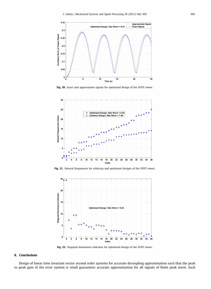
¼ 1=6, i¼ 1,:::,36.The decoupling approximation is not accurate and the algorithm has been applied to minimize the star norm. Theparameters used in SPSA were a¼10, S¼20, d¼0.1, b¼0.602, y¼0.101, resulting in an ‘‘optimized design’’ with a starnorm of Gf¼0.43 after 200 iterations which amounted to approximately 90 min of computation on the same computer.The energy gain is 0.26 and det Cnð Þ ¼�1:1e47. This design is characterized by

k1 ¼ 3:33, k2 ¼ 6:75, k3 ¼ 3:36, k4 ¼ 5:71, k5 ¼ 32:37, c1 ¼ 2:89, c2 ¼ 3:28, c3 ¼ 0:34, c4 ¼ 2:74: ð46Þ

The accuracy of the approximation is substantially improved, as indicated in Fig. 20 which shows the time histories ofthe exact and approximate output signal norms when the coupled and decoupled systems of the optimized design areexcited by the same signal as the arbitrary design. Fig. 21 shows that, similarly with the simplex and the two stage SVDTstructure, for the optimized design some frequencies are clustered (there are even identical, multiple frequencies). Fig. 22which shows the diagonal dominance indicator, Eq. (32), indicates that the modal damping matrix is not diagonallydominant.

Fig. 20. Exact and approximate signals for optimized design of the SVDT tower.

Fig. 21. Natural frequencies for arbitrary and optimized designs of the SVDT tower.

Fig. 22. Diagonal dominance indicator for optimized design of the SVDT tower.


8. Conclusions

Design of linear time invariant vector second order systems for accurate decoupling approximation such that the peakto peak gain of the error system is small guarantees accurate approximation for all signals of finite peak norm. Such


designs cover a large set of practically and theoretically relevant signals, including finite energy norm signals because thepeak to peak gain is larger than the energy gain. On the other hand computation of the peak to peak gain is expensivecompared to computation of the energy gain. Fortunately, an upper bound on the peak to peak gain, called the star norm,has very low computational complexity. When the simultaneous perturbation stochastic approximation is used for theminimization of the star norm over design parameters included in the system matrices, a reliable algorithm is obtained.The efficiency of this algorithm is illustrated on the design of tensegrity structures of increasing complexity: from asimplex structure with 6 generalized coordinates to an intricate tensegrity tower with 36 generalized coordinates.Reduction of the star norm of the error system to levels that provide accurate decoupling approximations was alwaysobtained.

Further investigation of the optimized designs thus achieved indicated that they do not have separated naturalfrequencies, some frequencies being clustered. Moreover, these designs do not have a diagonally dominant modal dampingmatrix either. Thus, for accurate decoupling approximation, neither separation of the natural frequencies nor diagonaldominance of the modal damping matrix is required. In addition, simulations for the simplex structure indicated that thedecoupled system for the optimized design may be used for accurate open loop tracking control of the original, coupledsystem. The quality of tracking can also be easily evaluated using system gains or the star norm. When closed loop (i.e.feedback) control design is pursued it may also be possible to obtain good results for the control of the original, coupledsystem using the decoupled system of the optimized design. However, an example included herein indicates that it is alsopossible that the quality of tracking degrades when the optimized design is used. This is explained by the fact that themathematical structure of the original, open loop system is significantly altered when feedback is used and thus the goodapproximation properties of the open loop system can be easily destroyed. If theoretical guarantees of good approximationare desired for the closed loop, a better approach may be to simultaneously design the physical system and the feedbackcontroller such that the approximation error for the closed loop is minimized. This can be a future research topic, whichalso depends on the structure of the controller to be implemented.

Acknowledgment

This material is based upon work supported by the National Science Foundation under the CAREER Grant no. CMMI-0952558.

References

[1] J.W.S. Rayleigh, The Theory of Sound, vol. I, Dover, New York, 1945 (reprint of the 1894 edition).[2] T.K. Caughey, Classical normal modes in damped linear structures, J. Appl. Mech. 27 (1960) 269–271.[3] T.K. Caughey, M.E.J. O’Kelly, Classical normal modes in damped linear dynamic systems, J. Appl. Mech. 32 (1965) 583–588.[4] A. Sestieri, S.R. Ibrahim, Analysis of errors and approximations in the use of modal co-ordinates, J. Sound Vib. 177 (2) (1994) 145–157.[5] F. Ma, A. Imam, M. Morzfeld, The decoupling of damped linear systems in oscillatory free vibration, J. Sound Vib. 324 (2009) 408–428.[6] R.W. Clough, S. Mojtahedi, Earthquake response analysis considering non-proportional damping, Earthquake Eng. Struct. Dyn. 4 (1976) 489–496.[7] F. Ma, T.K. Caughey, Analysis of linear nonconservative vibrations, ASME J. Appl. Mech. 62 (1995) 685–691.[8] F. Ma, M. Morzfeld, A. Imam, The decoupling of damped linear systems in free or forced vibration, J. Sound Vib. 329 (2010) 3182–3202.[9] D.T. Kawano, M. Morzfeld, F. Ma, The decoupling of defective linear dynamical systems in free motion, J. Sound Vib. 330 (2011) 5165–5183.

[10] F. Ma, M. Morzfeld, The decoupling of damped linear systems in configuration and state spaces, J. Sound Vib. 330 (2011) 155–161.[11] S.D. Garvey, M.I. Friswell, U. Prells, Coordinate transformations for second order systems, part I: general transformations, J. Sound Vib. 258 (5) (2002)

885–909.[12] S.D. Garvey, M.I. Friswell, U. Prells, Coordinate transformations for second order systems, part II: elementary structure-preserving transformations,

J. Sound Vib. 258 (5) (2002) 911–930.[13] M.T. Chu, N. DelBuono, Total decoupling of general quadratic pencils, J. Sound Vib. 309 (2008) 96–111.[14] M.T. Chu, N. DelBuono, Total decoupling of general quadratic pencils, part II: structure preserving isospectral flows, J. Sound Vib. 309 (2008)

112–128.[15] S.M. Shahruz, Comments on an index of damping non-proportionality for discrete vibrating systems, J. Sound Vib. 186 (3) (1995) 535–542.[16] M. Tong, Z. Liang, G.C. Lee, An index of damping non-proportionality for discrete vibrating systems, J. Sound Vib. 174 (1994) 37–55.[17] J.K. Knowles, On the approximation of damped linear dynamical systems, Struct. Control Health Monitor. 13 (2006) 324–335.[18] F.E. Udwadia, A note on non-proportional damping, J. Eng. Mech. 135 (11) (2009) 1248–1256.[19] M. Morzfeld, N. Ajavakom, F. Ma, Diagonal dominance of damping and the decoupling approximation in linear vibratory systems, J. Sound Vib. 320

(2009) 406–420.[20] W.K. Gawronski, J.T. Sawicki, Response errors of non-proportionally lightly damped structures, J. Sound Vib. 200 (4) (1997) 543–550.[21] W.K. Gawronski, Advanced Structural Dynamics and Active Control of Structures, Springer, New York, NY, USA, 2004.[22] S. Park, I. Park, F. Ma, Decoupling approximation of non-classically damped structures, AIAA J. 30 (9) (1992) 2348–2351.[23] S.M. Shahruz, A.K. Packard, Approximate decoupling of weakly damped linear second-order systems under harmonic excitations, in: Proceedings

of the IEEE Conference on Decision and Control, Tucson, AZ, USA, 1992.[24] S.M. Shahruz, G. Langari, Closeness of the solutions of approximately decoupled damped linear systems to their exact solutions, Trans. ASME J. Dyn.

Syst. Meas. Control 114 (1992) 369–374.[25] S. Park, I. Kim, F. Ma, Characteristics of modal decoupling in non-classically damped systems under harmonic excitation, J. Appl. Mech. 61 (1994)

77–83.[26] S.M. Shahruz, A.K. Packard, Approximate decoupling of weakly non-classically damped linear second-order systems under harmonic excitations, J.

Dyn. Syst. Meas. Control-Trans. ASME 115 (1993) 214–218.[27] S. Adhikari, Optimal complex modes and an index of damping non-proportionality, Mech. Syst. Signal Process. 18 (2004) 1–24.[28] U. Prells, M.I. Friswell, A measure of non-proportional damping, Mech. Syst. Signal Process. 14 (2) (1999) 125–137.[29] J. Angeles, S. Ostrovskaya, The proportional-damping matrix of arbitrarily damped linear mechanical systems, ASME J. Appl. Mech. 69 (5) (2002)

649–656.[30] M.P. Bendsoe, A. Ben-Tal, J. Zowe, Optimization methods for truss geometry and topology design, Struct. Optim. 7 (1994) 141–159.


[31] Special issue on multidisciplinary design optimization, J. Aircr. 36 (1) (1999).[32] N.L. Pedersen, Optimization of holes in plates for control of eigenfrequencies, Struct. Multidiscip. Optim. 28 (1) (2004) 1–10.[33] N.L. Pedersen, On simultaneous shape and orientation design for eigenfrequencies optimization, Struct. Multidiscip. Opt. 33 (4–5) (2007) 387–399.[34] O. Sergeyev, Z. Mroz, Sensitivity analysis and optimal design of 3D frame structures for stress and frequencies constraints, Comput. Struct. 75 (2)

(2000) 167–185.[35] J. Sobieszczanski-Sobieski, R.T. Haftka, Multidisciplinary aerospace design optimization: survey of recent developments, Struct. Multidiscip. Optim.

14 (1) (1997) 1–23.[36] R.W. Wlezien, G.C. Horner, A.R. McGowan, S.L. Padula, M.A. Scott, R.J. Silcox, J.O. Simpson, The aircraft morphing program, AIAA paper AIAA-1998-

1927, in Proceedings of the AIAA/ASME/ASCE/AHS/ASC Structures, Structural Dynamics, and Materials Conference and Exhibit, Long Beach, CA, 1998.[37] B.F. Spencer Jr., S. Nagarajaiah, State of the art of structural control, J. Struct. Eng. 129 (7) (2003) 845–856.[38] S.K. Dwivedy, P. Eberhard, Dynamic analysis of flexible manipulators, a literature review, Mech. Mach. Theory 41 (7) (2006) 749–777.[39] A.J. Laub, W.F. Arnold, Controllability and observability criteria for multivariable linear second order models, IEEE, Trans. Autom. Control 29 (2)

(1984) 163–165.[40] G.M.L. Gladwell, Inverse Problems Vibrations, Martinus Nijhoff, Boston, MA, USA, 1986.[41] L. Starek, D.J. Inman, A. Kress, A symmetric inverse vibration problem, Trans. ASME J. Vib. Acoust. 114 (1992) 564–568.[42] L. Starek, D.J. Inman, A symmetric inverse vibration problem for non-proportional, underdamped system, ASME J. Appl. Mech. 64 (1997) 601–605.[43] L. Starek, D.J. Inman, Symmetric inverse eigenvalue vibration problem and its application, Mech. Syst. Signal Process. 15 (1) (2001) 11–29.[44] P. Lancaster, J. Maroulas, Inverse eigenvalue problems for damped vibrating systems, J. Math. Anal. Appl. 123 (1987) 238–261.[45] P. Lancaster, U. Prells, Inverse problems for damped vibrating systems, J. Sound Vib. 283 (2005) 891–914.[46] P. Lancaster, Inverse spectral problems for semi-simple damped vibrating systems, SIAM J. Matrix Anal. 29 (1) (2007) 279–301.[47] J.S. Jensen, N.L. Pedersen, On maximal eigenfrequency separation in two material structures: the 1D and 2D scalar cases, J. Sound Vib. 289 (2006)

967–986.[48] N.L. Pedersen, A.K. Nielsen, Optimization of practical trusses with constraints on eigenfrequencies, displacements, stresses and buckling, Struct.

Multidiscip. Optim. 25 (2003) 436–445.[49] C. Sultan, Designing structures for dynamic properties via natural frequencies separation; application to tensegrity structures design, Mech. Syst.

Signal Process. 23 (4) (2009) 1112–1122.[50] C. Sultan, Proportional damping approximation using the energy gain and simultaneous perturbation stochastic approximation, Mech. Syst. Signal

Process. 24 (6) (2010) 2210–2224.[51] J. Abedor, K. Nagpal, K. Poola, A linear matrix inequality approach to peak-to-peak gain minimization, Int. J. Robust Nonlinear Control 6 (1996)

899–927.[52] N. Hovakimyan, C. Cao, L1 Adaptive Control Theory, SIAM, USA, 2010.[53] S. Adhikari, Damping modeling using generalized proportional damping, J. Sound Vib. 293 (2006) 156–170.[54] S. Boyd, L. El Ghaoui, E. Feron, V. Balakrishnan, Linear Matrix Inequalities in System and Control Theory, SIAM, Philadelphia, 1994.[55] M. Corless, A. Frazho, Linear Systems and Control: An Operator Perspective, Decker, 2009.[56] J.C. Spall, Implementation of the simultaneous perturbation algorithm for stochastic optimization, IEEE Trans. Aerosp. Electron. Syst. 34 (1998)

817–823.[57] J.C. Spall, Multivariable stochastic approximation using a simultaneous perturbation gradient approximation, IEEE Trans. Autom. Control 37 (1992)

332–341.[58] C. Sultan, Tensegrity: sixty years of art, science, and engineering, Adv. Appl. Mech. 43 (2009) 69–145.[59] C. Sultan, M. Corless, R.E. Skelton, Symmetrical reconfiguration of tensegrity structures, Int. J. Solids Struct. 39 (8) (2002) 2215–2234.[60] C. Sultan, R.E. Skelton, Linearized dynamics of tensegrity structures, Eng. Struct. 26 (6) (2002) 671–685.[61] C. Sultan, Tensegrity motion control using internal mechanisms, in: Proceedings of the Conference on Control Applications, St. Petersburg, Russia,

2009.[62] C. Sultan, M. Corless, R.E. Skelton, The prestressability problem of tensegrity structures. Some analytical solutions, Int. J. Solids Struct. 38–39 (2001)

5223–5252.[63] C. Sultan, R.E. Skelton, Tensegrity structures prestressability investigation, Int. J. Space Struct. 18 (1) (2003) 15–30.

Date post:	05-Jan-2017
Category:	Documents
Upload:	cornel
View:	215 times
Download:	3 times

Decoupling approximation design using the peak to peak gain

Documents