HAL Id: hal-02994705 https://hal.archives-ouvertes.fr/hal-02994705 Submitted on 25 Oct 2021 HAL is a multi-disciplinary open access archive for the deposit and dissemination of sci- entific research documents, whether they are pub- lished or not. The documents may come from teaching and research institutions in France or abroad, or from public or private research centers. L’archive ouverte pluridisciplinaire HAL, est destinée au dépôt et à la diffusion de documents scientifiques de niveau recherche, publiés ou non, émanant des établissements d’enseignement et de recherche français ou étrangers, des laboratoires publics ou privés. Distributed under a Creative Commons Attribution - NonCommercial| 4.0 International License Decoupling multivariate polynomials: Interconnections between tensorizations Konstantin Usevich, Philippe Dreesen, Mariya Ishteva To cite this version: Konstantin Usevich, Philippe Dreesen, Mariya Ishteva. Decoupling multivariate polynomials: Inter- connections between tensorizations. Journal of Computational and Applied Mathematics, Elsevier, 2020, 363, pp.22-34. 10.1016/j.cam.2019.03.036. hal-02994705
Transcript
HAL Id: hal-02994705https://hal.archives-ouvertes.fr/hal-02994705
Submitted on 25 Oct 2021
HAL is a multi-disciplinary open accessarchive for the deposit and dissemination of sci-entific research documents, whether they are pub-lished or not. The documents may come fromteaching and research institutions in France orabroad, or from public or private research centers.
L’archive ouverte pluridisciplinaire HAL, estdestinée au dépôt et à la diffusion de documentsscientifiques de niveau recherche, publiés ou non,émanant des établissements d’enseignement et derecherche français ou étrangers, des laboratoirespublics ou privés.
Distributed under a Creative Commons Attribution - NonCommercial| 4.0 InternationalLicense
Konstantin Usevich, Philippe Dreesen, Mariya Ishteva
To cite this version:Konstantin Usevich, Philippe Dreesen, Mariya Ishteva. Decoupling multivariate polynomials: Inter-connections between tensorizations. Journal of Computational and Applied Mathematics, Elsevier,2020, 363, pp.22-34. �10.1016/j.cam.2019.03.036�. �hal-02994705�
Konstantin Usevicha,∗, Philippe Dreesenb, Mariya Ishtevab3
aUniversite de Lorraine, CNRS, CRAN, F-54000 Nancy, France4
bVrije Universiteit Brussel (VUB), Department VUB-ELEC, Brussels, Belgium5
Abstract6
Decoupling multivariate polynomials is useful for obtaining an insight into the workings7
of a nonlinear mapping, performing parameter reduction, or approximating nonlinear8
functions. Several different tensor-based approaches have been proposed independently9
for this task, involving different tensor representations of the functions, and ultimately10
leading to a canonical polyadic decomposition.11
We first show that the involved tensors are related by a linear transformation, andthat their CP decompositions and uniqueness properties are closely related. This con-nection provides a way to better assess which of the methods should be favored in certainproblem settings, and may be a starting point to unify the two approaches. Second, weshow that taking into account the previously ignored intrinsic structure in the tensor de-compositions improves the uniqueness properties of the decompositions and thus enlargesthe applicability range of the methods.
In this paper, we focus on the task of decoupling a set of polynomial vector functions,25
that is, decomposing a set of multivariate real polynomials into linear combinations of26
univariate polynomials in linear forms of the input variables. This task has attracted a27
spark of research attention over the last years, motivated by several applications, such as28
system identification [9, 10, 11, 12, 13, 14], approximation theory [15, 16, 17], and neural29
networks [18]. Restricting polynomial decoupling to a single homogeneous polynomial is30
equivalent to the well-known Waring decomposition [19, 20], but some generalizations to31
non-homogeneous polynomials or joint Waring decompositions are studied as well [21, 22]32
and [23, 24, 11].33
Several tensor-based approaches were proposed for computing a decoupled represen-34
tation of a given function [12, 13, 25, 26, 24]. These solutions can be categorized into35
two classes. The methods [12, 13, 25, 26] build a tensor from the polynomial coefficients,36
whereas the method of [24] builds a tensor from the Jacobian matrices of the functions,37
evaluated at a set of sampling points. Ultimately, all methods boil down to a canon-38
ical polyadic decomposition (CP decomposition) of the constructed tensor to retrieve39
a decoupled representation in which the nonlinearities occur as univariate polynomial40
mappings.41
The benefit of using a tensor-based approach for decoupling is twofold. First, ‘ten-42
sorization’ procedures often lead to (essentially) uniquely decomposable tensors [8], i.e.,43
ensuring that identifiable structures can be retrieved. Second, by solving the decoupling44
problem as a CP decomposition, one can use recent widely available and robust numerical45
tools, such as Tensorlab for MATLAB [27] (or alternatives [28, 29]).46
This paper specifically focuses on the two tensorization methods [26] and [24]. Al-47
though both associated tensors have a particular structure, both approaches seem quite48
different in nature, and each of the methods has distinct advantages over the other one.49
For instance, the coefficient-based methods [12, 13, 25, 26] require several high-order50
tensors (or their matricizations) for polynomials of high degrees, whereas [24] involves a51
single third-order tensor only. Coefficient-based approaches can easily deal with single52
polynomials, whereas [24] would in that case not be able to take advantage of the unique-53
ness properties of the CP decomposition, as the tensor of Jacobian matrices is then a54
matrix composed of gradient vectors. On the other hand, the approach of [24] can be55
applied to non-polynomial functions, which may in some cases be of interest, e.g., in [9]56
a neural network was decoupled.57
We aim at obtaining a deeper understanding of the connections between the solution58
approaches. This is profitable when extending the applicability range of the methods,59
e.g., when moving from polynomials to any differentiable functions. Furthermore, such60
connections may provide a way to transfer theoretical properties from one formulation to61
another. For example, as we argue in Section 6, exploring the previously ignored structure62
in the tensor decomposition in one of the settings enlarges the range of decomposable63
functions. This knowledge may lead to improved algorithms in another setting as well.64
The remainder of this article is organized as follows: Section 2 formalizes the problem65
of decoupling multivariate polynomials. Section 3 explains the link between the decou-66
pling problem and the symmetric tensor decomposition problem. Section 4 discusses67
the construction of the tensor of unfoldings [26] and the Jacobian tensor [24]. Section 568
presents our first contribution, namely the relation between the two tensorizations. The69
second main contribution of the paper is Section 6, which clarifies the need of dealing70
with structure in the decompositions and proposes a coupled CP decomposition approach71
2
for solving the structured problem. Section 7 draws the conclusions and points out open72
problems for future work.73
Notation74
Scalars are denoted by lowercase or uppercase letters. Vectors are denoted by low-75
ercase boldface letters, e.g., u. Elements of a vector are denoted by lowercase letters76
with an index as subscript, e.g., x =[x1 · · · xm
]>. Matrices are denoted by up-77
percase boldface letters, e.g., V. The entry in the i-th row and j-th column of a matrix78
V is denoted by vij , and the matrix V ∈ Rm×r may be represented by its columns79
V =[v1 · · · vr
]. The Kronecker product of matrices is denoted by “⊗”.80
Tensors of order d are denoted by uppercase caligraphical letters, e.g., J ∈ Rn×m×N .81
The outer product is denoted by “◦” and is defined as follows: For T = u ◦ v ◦w, the82
entry in position (i, j, k) is equal to uivjwk. The canonical polyadic (CP) decomposition83
expresses a tensor T as a (minimal) sum of rank-one tensor terms [30, 31, 2] as T =84 ∑Ri=1 ui ◦vi ◦wi, and is sometimes denoted in a short-hand notation as T = JU,V,WK.85
The CP rank r is defined as the (minimal) number of terms that is required to represent86
T as a sum of r rank-one terms. To refer to elements of matrices or tensors, or subsets87
thereof, we may use MATLAB-like index notation (including MATLAB’s colon wildcard):88
for instance, Ti,j,k,` is the element at position (i, j, k, `) of a fourth-order tensor T , and89
T:,:,2 is the second frontal slice of a third-order tensor T . The mode-n product is denoted90
by “•n” and is defined as follows. Let X be an I1 × I2 × · · · × IN tensor, and let u be a91
vector of length In, then we have(X •n u>
)i1···in−1in+1···iN
=∑Inin=1 xi1i2···iNuin . Notice92
that the result is a tensor of order N − 1, as mode n is summed out. Similarly, for an93
I1 × I2 × · · · × IN tensor X and a matrix M ∈ J × In, the mode-n product is defined94
as(X •n M>
)i1···in−1jin+1···iN
=∑Inin=1 xi1i2···iNmj,in . Let vec(T ) denote the column-95
major vectorization of a tensor T . The first-mode unfolding of an I1 × I2 × · · · × IN96
tensor X is the matrix X(1) of size I1 × I2 · · · IN , where each row is the vectorized slice97
of the tensor X , i.e. (X(1))i,: = (vec(Xi,:,...,:))> (see, for example, [2] for more details).98
2. The polynomial decoupling model99
First, we describe the model, following the notation of [24] as illustrated in Fig. 1.100
Consider a multivariate polynomial map f : Rm → Rn, i.e., a vector101
f(u) =[f1(u) · · · fn(u)
]>of multivariate polynomials (of total degree at most d) in variables u =
[u1 · · · um
]>.102
We say that f has a decoupled representation, if it can be expressed as103
f(u) = Wg(V>u), (1)
where V ∈ Rm×r,W ∈ Rn×r are transformation matrices, and g : Rr → Rr is defined as104
g(x1, . . . , xr) =[g1(x1) · · · gr(xr)
]>,
where gk : R→ R are univariate polynomials of degree at most d, i.e.,105
gk(t) = c1t+ · · ·+ cdtd. (2)
3
Note that we omitted the constant terms of the polynomials, since they are not uniquely106
identifiable [24]. In this paper we limit ourselves to the model (1).
u1
...
um
f(u1, . . . , um)
y1
...
yn
=
u1
...
um
V>
g1(x1)x1
...
gr(xr)xr
W
z1
zr
y1
...
yn
Figure 1: Every multivariate polynomial vector function f(u) can be represented by a linear transfor-mation of a set of univariate functions (in linear combinations of the original variables).
107
The decoupled representation (1) can be also equivalently rewritten as108
f(u) = w1g1(v>1 u) + · · ·+ wrgr(v>r u), (3)
where vk and wk are the columns of V and W, respectively. As shown in [32, 33], the109
decomposition (3) is a special case of the X-rank decomposition [34, §5.2.1], where the110
set of “rank-one” terms is the set of polynomial maps of the form wg(v>u). The X-rank111
framework is useful [33] for studying the identifiability of the model (3).112
The following example shows a decoupled representation for a simple case. This113
example will be used throughout the paper to illustrate the main ideas of the various114
aspects that we will explore.115
Example 1. Consider a function f(u) =[f1(u1, u2) f2(u1, u2)
Remark 1. In general, the coupled representation f(u) has n((m+dd
)− 1)
coefficients,120
while the decoupled representation Wg(V>u) has r(m+ n+ d) coefficients. Due to the121
combinatorial increase of the number of coefficients in the coupled representation, the122
decoupled representation is especially beneficial for large values of m, n, and d. But even123
for small values of m, n, and d, the parametric reduction can be significant, for example,124
if m = n = 3, d = 5, and r = 3, the coupled representation has 168 coefficients, while125
the decoupled one has only 36 coefficients.126
4
-5000
-5
0
5000
u1
0
u2
55 0
-5
-500
0
-5
500
1000
u1
0
u2
55 0
-5
-5 0 5
x1
-300
-150
0
150
-5 0 5
x1
-300
-150
0
150
-5 0 5
x1
-150
0
150
300
Figure 2: The decoupling problem in Example 1 consists of decomposing the multivariate functionsf1(u1, u2) and f2(u1, u2) (top row) to the univariate functions g1(x1), g2(x2), and g3(x3) (bottom row),using suitable transformation matrices as in (1).
3. Decoupling polynomials and symmetric tensor decompositions127
Let us review some well-known facts that connect polynomials with symmetric tensors128
[35, 36], and that connect some special cases of the representation (1) with symmetric129
tensor decompositions.130
3.1. Homogeneous polynomials, symmetric tensors and Waring decomposition131
It is well-known that there is a one-to-one correspondence between homogeneous132
polynomials and symmetric tensors [35]. For instance, the polynomial −8u21 − 8u1u2 −133
20u22 can be written as134
− 8u21 − 8u1u2 − 20u22 = u>Ψ(2)u, where Ψ(2) =
[−8 −4−4 −20
]. (4)
In general, let p(d)(u1, . . . , um) be a homogeneous polynomial (also called a d-ary form)135
of degree d in m variables. Then there is a unique symmetric tensor Ψ(d) of order d and136
dimension m such that137
p(u) = Ψ(d) •1 u · · · •d u. (5)
Next, it is easy to see that the decoupling problem for the polynomial (5) takes the form138
p(u1, . . . , um) =
r∑i=1
wi(v1iu1 + · · ·+ vmium)d, (6)
5
which is known as the Waring decomposition [19, 20] of p(u1, . . . , um). The Waring139
decomposition, in its turn, is equivalent to the symmetric CP decomposition of Ψ(d):140
Ψ(d) =
r∑i=1
wi(vi ◦ · · · ◦ vi).
The symmetric CP decomposition of Ψ(d) reveals possible values for the unknowns vij141
and wi.142
Example 2. Consider the polynomial given in (4). Then the corresponding symmetric143
matrix Ψ(2) admits the decomposition144 [−8 −4−4 −20
]=
[−2 2
2 4
] [−1 0
0 −1
] [−2 2
2 4
], (7)
such that p(u1, u2) = u>Ψ(2)u has the Waring decomposition145
p(u1, u2) = −(−2u1 + 2u2)2 − (2u1 + 4u2)2.
Notice that the symmetric decomposition of Ψ(2) from Example 2 is not unique (nor146
‘essentially unique’ [2]). Indeed, the eigenvalue decomposition147 [−8 −4−4 −20
]≈[
0.2898 −0.95710.9571 0.2898
] [−21.2111 0
0 −6.7889
] [0.2898 0.9571−0.9571 0.2898
]provides another valid factorization. For d > 2, however, the Waring decomposition (6)148
possesses uniqueness properties even in the case of quite large ranks [37, 38].149
Along the same lines, it is possible to decouple jointly several homogeneous polyno-150
mials. Consider the case of n homogeneous polynomials of degree d, denoted by151
p1(u1, . . . , um) = Ψ(d)1 •1 u · · · •d u,
...
pn(u1, . . . , um) = Ψ(d)n •1 u · · · •d u.
(8)
Then the decoupling problem (1) corresponds to the simultaneous Waring decomposition152
of several forms or, equivalently, the coupled CP decomposition of several symmetric153
tensors. The rank and identifiability properties of simultaneous Waring decompositions154
were also studied in the literature, see [23, 37, 39] and references therein.155
3.2. The case of non-homogeneous polynomials156
Next, consider the case of non-homogeneous polynomials. Any non-homogeneous157
polynomial of degree d can hence be written as158
p(u) = u>Ψ(1) + u>Ψ(2)u + Ψ(3) •1 u •2 u •3 u + · · ·+ Ψ(d) •1 u · · · •d u, (9)
where Ψ(1) ∈ Rm , Ψ(2) ∈ Rm×m is a symmetric matrix, and each Ψ(s) ∈ Rm×···×m,159
3 ≤ s ≤ d, is a symmetric tensor of order s.160
6
Example 3. We continue Example 1. We can write f1(u1, u2) and f2(u1, u2) as161
f1(u1, u2) = u>[
39
]+ u>
[−8 −4−4 −20
]u + Ψ(3) •1 u •2 u •3 u,
with162
Ψ(3):,:,1 =
[−3 −3−3 −9
], Ψ
(3):,:,2 =
[−3 −9−9 −15
],
and163
f2(u1, u2) = u>[
0−3
]+ u>
[10 88 10
]u + Ψ(3) •1 u •2 u •3 u,
with164
Ψ(3):,:,1 =
[−7 −2−2 2
], Ψ
(3):,:,2 =
[−2 2
2 7
].
The decomposition of a single non-homogeneous polynomial as in (3) is hence equiv-165
alent to joint decomposition of several symmetric tensors but of different orders [32].166
Finally, several non-homogeneous polynomials can be jointly decomposed in a similar167
way. Consider n non-homogeneous polynomials of maximal degree d, denoted as168
p1(u1, . . . , um) = u>Ψ(1)1 + · · ·+ Ψ
(d)1 •1 u · · · •d u,
...
pn(u1, . . . , um) = u>Ψ(1)n + · · ·+ Ψ
(d)n •1 u · · · •d u,
(10)
The full decomposition in (1) can be also viewed as a coupled tensor decomposition,169
which will be presented in Section 6.2.170
4. Tensorizations and their decompositions171
In this section, we recall tensorizations proposed in the literature to find the decom-172
position (1) by a CP decomposition of a single tensor constructed from f , namely the173
tensorizations of [26] and [24]. We recall basic properties and give short proofs for com-174
pleteness, although these proofs are already present in [26, 24]. We also use a slightly175
different notation to simplify the exposition.176
4.1. Tensor of unfoldings [26]177
The above link between polynomials, (partially) symmetric tensors and their CP178
decompositions gives rise to the tensorization approach of [26], in which a tensor is179
constructed from the coefficients of the polynomials f1(u1, . . . , um) up to fn(u1, . . . , um).180
This tensorization offers the advantage that several polynomials can be represented as a181
single tensor, and the decoupling task can be solved using a single (but structured) CP182
decomposition. In this approach, the tensor (shown in Figure 3) is constructed from the183
coefficients of the polynomial map of degree d, as follows:184
• The tensor has size n×m× δ, where δ =d∑k=1
mk−1.185
7
• The tensor is constructed by slices186
Qi,:,: := Ψ(fi),
where Ψ is a structured m× δ matrix built from the coefficients of fi(u).187
=Q ...
Ψ(f1)
Ψ(f2)
Ψ(fn)m
n
δ
Figure 3: The coefficients of a polynomial map f : Rm → Rn of degree d can be arranged into ann×m× δ tensor Q, where δ =
∑dk=1m
k−1.
Now let us describe the construction of the structured coefficient matrix Ψ(p) for a188
given polynomial of degree d. Recall that each such polynomial can be written as in189
(9), where Ψ(1) ∈ Rm , Ψ(2) ∈ Rm×m is a symmetric matrix and Ψ(s) ∈ Rm×···×m are190
symmetric tensors of order s. Then the matrix Ψ(p) ∈ Rm×δ is constructed1 as191
Ψ(p) =[
Ψ(1) Ψ(2) Ψ(3)(1) · · · Ψ
(d)(1)
], (11)
where G(1) denotes the first-mode unfolding of a tensor G.192
Example 4. A third-degree polynomial in two variables193
Hence, for f1 and f2 in Example 1, the slices of the tensor Q are given by197
Q1,:,: = Ψ(f1) =
[3 −8 −4 −3 −3 −3 −99 −4 −20 −3 −9 −9 −15
],
1In [26] the linear term is skipped, and δ =d∑
k=2md−1. In [40] the matrix Ψ is denoted as Γ.
8
and198
Q2,:,: = Ψ(f2) =
[0 10 8 −7 −2 −2 2−3 8 10 −2 2 2 7
].
As proved in [26], the tensor Q has a CP decomposition, which reveals the decompo-199
sition (1). We repeat here a simplified version of the proof for completeness.200
Lemma 1. For the polynomial map (1), the tensor Q has the following CP decomposi-201
tion:202
Q =
r∑k=1
wk ◦ vk ◦ zk, (14)
where203
zk =[ck,1 ck,2v
>k ck,3(vk ⊗ vk)> · · · ck,d(vk ⊗ · · · ⊗ vk)>
]>. (15)
Proof. Consider qk(u) := gk(v>k u), where gk is as in (2). Easy calculations show that204
Ψ(qk) = vkz>k ,
see also [40, eqn. (A.7)]. Since, from (3) fi(u) =r∑
k=1
(wk)iqk(u), we have that205
Ψ(fi) =
r∑k=1
(wk)ivkz>k
which implies (14).206
Example 5. We continue Examples 1, 4. The Kronecker products of columns of V are:207
(v1⊗v1)> =[4 2 2 1
], (v2⊗v2)> =
[1 −1 −1 1
], (v3⊗v3)> =
[1 2 2 4
].
Hence, the matrix Z =[z1 z2 z3
]is given by208
Z> =
−1 −4 −2 4 2 2 11 4 −4 1 −1 −1 1−2 2 4 1 2 2 4
.4.2. The tensor of Jacobian matrices of [24]209
The tensorization method of [24] does not use the coefficients of f(u) directly, but210
proceeds by collecting the first-order information of f(u) (i.e., the partial derivatives)211
in a set of sampling points. The thusly obtained Jacobian matrices are arranged into a212
third-order tensor, of which the CP decomposition reveals the decomposition (1).213
As in [24], we consider the Jacobian of f :214
Jf (u) :=
∂f1∂u1
(u) · · · ∂f1∂um
(u)...
...∂fn∂u1
(u) · · · ∂fn∂um
(u)
. (16)
Using Lemma 2, the tensorization is constructed as follows (see Figure 4):215
9
• N points u(1), . . . ,u(N) ∈ Rm are chosen (so-called sampling points).216
• An n×m×N tensor J is constructed by stacking the Jacobian evaluations at u(k)217
J:,:,k := Jf (u(k)).
=J
J(u1)J(u2)
J(uN )
. ..
m
n
N
Figure 4: The third-order tensor J is constructed by stacking behind each other a set of Jacobianmatrices J evaluated at the sampling points u(k). Its CP decomposition is equivalent to joint matrixdiagonalization of the Jacobian matrix slices.
Example 6. We continue Example 1. As a set of sampling points, we choose218
u =
[00
],u(2) =
[10
],u(3) =
[01
].
By evaluating Jf (u) at these points, we get the tensor J given by219
J:,:,1 =
[3 90 −3
], J:,:,2 =
[−22 −8−1 7
], J:,:,3 =
[−32 −7622 38
]. (17)
If f(u) has a decoupled representation (1), the following lemma holds true.220
Lemma 2 ([24, Lemma 2.1]). The first order derivatives of (1) are given by221
Earlier attempts to tackle the structured case were made by [25, 13] and [42, §8,320
pp. 133–136]. The attempts of [25, 13] have the disadvantage that a tensor is built321
that has missing values, which increase in number as the polynomial degree grows. The322
attempt of [42] consisted of parameterizing the internal nonlinear functions gk using their323
coefficients. Although this seems a promising approach, it turned out to be problematic324
in practice to build a working algorithm, as the decoupling method led to strongly325
nonlinear/nonconvex optimization problems.326
We propose to tackle the problem by solving a coupled and structured CP decomposi-327
tion instead. First, let us consider simultaneous decoupling of homogeneous polynomials328
(8). Let us arrange the Ψ(d)i , for i = 1, . . . , n into a tensor T d, such that T di,:,...,: = Ψ
(d)i ,329
for all i = 1, . . . , n. Then it is easy to verify that T d admits a partially symmetric CP330
decomposition331
T d = JW,V, . . . ,V︸ ︷︷ ︸d times
K,
which, in our decoupled representation (1), takes the form Wg(V>u), where g(x) =332 [xd1 · · · xdr
]>.333
Decoupling non-homogeneous polynomials can be achieved by means of a coupled334
structured CP decomposition of the T d tensors. Let us arrange all Ψ(d)i , for i = 1, . . . , n335
into the tensors T d (like in the previous paragraph), such that T di,:,...,: = Ψ(d)i , for all i =336
1, . . . , n. We now have for each degree a coupled partially symmetric CP decomposition337
as338
T 1 = JW,V, c>1 K,T 2 = JW,V,V, c>2 K,
...T d = JW,V, . . . ,V︸ ︷︷ ︸
d times
, c>d K,(30)
where the ci, for i = 1, . . . , d, are the i-th degree coefficients for each of the r nonlinear339
functions gk.340
Remark that these coefficients were not required in the previous paragraphs when341
homogeneous polynomials were considered: in such cases the nonlinear functions gk are342
of the form cktd, i.e., they differ only by a scaling factor, which can be assumed to be fully343
absorbed by W. Also remark that there are redundancies in the representation (30):344
for example, an equivalent problem can be obtained if one rescales a coefficient vector cδ345
to a vector containing ones, in which case a rescaling has to take place on the remaining346
coefficients as well as on W. Finally we want to mention that the framework of structured347
data fusion [43, 27] allows for computing tensor decompositions as in (30), where several348
tensors (and possibly matrices) are jointly decomposed while sharing factors, possibly349
while imposing structure on the factors.350
Example 9. Let us continue with Examples 1, 6 and 7. We have that m = n = 2 and351
r = 3, which does not guarantee a unique CP decomposition of J (under assumptions352
of genericity, see [24]). Indeed, if we compute a numerical CP decomposition of ten-353
sor J , we find that, up to a relative norm-wise error 2.3546 × 10⁻¹⁶, J admits a CP354
15
decomposition with factors355
W =
[1.1628 −3.2951 3.02520.5705 1.1349 −2.1791
], V =
[3.5822 −0.7705 −2.2959−0.0226 −3.4455 −2.9785
],
H =
0.2736 0.8181 0.0312−3.3900 0.2647 1.2313
0.5334 −3.9194 3.4945
,the columns of which are not scaled and permuted versions of the columns of W, V, H.356
It can be shown that the ‘structured CP’ approaches are able to correctly return the357
underlying factors W, V and H (up to scaling and permutation invariances). For in-358
stance, the structured data fusion framework [43, 27] is able to compute the coupled and359
partially symmetric decomposition (30). This returns360
W =
[1.2767 1.7112 0
0 −0.8556 −1.9980
], V =
[−0.9218 −1.0534 1.5879
0.9218 −2.1067 0.7940
],
as well as computed values for the coefficient vectors of gi(xi), which are omitted here.361
It can be verified that W and V are scaled and permuted versions of W and V.362
Remark that if one uses m = n = r = 2, both the structured and non-structured363
CP decomposition return the same decomposition (up to scaling and permutation of the364
columns of the factors). Indeed, in this case, uniqueness is guaranteed (generically),365
ensuring that the underlying factors are identifiable. This could be checked easily by366
generating a variation of the equations that we are decoupling where the third columns of367
V and W are removed, so that g3(x3) is not considered.368
6.3. Linking Q and T 1, . . . , T d tensors369
In this section, we show how Q and its CPD is connected with the tensors T s and370
their joint decomposition (30). Let (1, 2)-reshapings of the tensors T s to be the third371
order tensors T s(1,2) ∈ Rn×m×ms−1
defined as372
(T s(1,2))i,j,: = vec(T si,j,:,··· ,:).
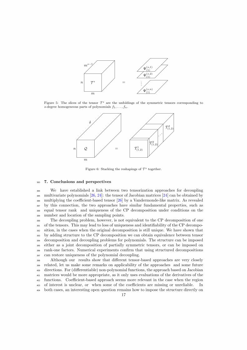
Then it is easy to see that the tensor T s(1,2) can be split into slices as shown in Fig. 5,373
where the Ψ(s,j) is the symmetric tensor corresponding to the s-th degree homogeneous374
part of the polynomial fk.375
By taking into account the definition (11) of the slices of the tensor Q, we can easily376
see that Q can be constructed by stacking the tensors is equivalent to reshaping the377
tensors T s(1,2) along the third mode together, as shown in Fig. 6.378
Remark that in Lemma 1 we see that the structure appearing in the CP decomposition379
of Q is closely connected to the simultaneous decomposition described in Section 6.2.380
Indeed, Lemma 1 can be alternatively deduced from (30), because the outer products of381
vectors become Kronecker products after reshaping.382
16
=T s ...
Ψ(s,1)
(1)
Ψ(s,2)
(1)
Ψ(s,n)
(1)m
n
ms−1
Figure 5: The slices of the tensor T s are the unfoldings of the symmetric tensors corresponding tos-degree homogeneous parts of polynomials f1, . . . , fn.
=Q T 1(1,2)
T 2(1,2)
. ..
T d(1,2)
m
n
δ
Figure 6: Stacking the reshapings of T s together.
7. Conclusions and perspectives383
We have established a link between two tensorization approaches for decoupling384
multivariate polynomials [26, 24]: the tensor of Jacobian matrices [24] can be obtained by385
multiplying the coefficient-based tensor [26] by a Vandermonde-like matrix. As revealed386
by this connection, the two approaches have similar fundamental properties, such as387
equal tensor rank and uniqueness of the CP decomposition under conditions on the388
number and location of the sampling points.389
The decoupling problem, however, is not equivalent to the CP decomposition of one390
of the tensors. This may lead to loss of uniqueness and identifiability of the CP decompo-391
sition, in the cases when the original decomposition is still unique. We have shown that392
by adding structure to the CP decomposition we can obtain equivalence between tensor393
decomposition and decoupling problems for polynomials. The structure can be imposed394
either as a joint decomposition of partially symmetric tensors, or can be imposed on395
rank-one factors. Numerical experiments confirm that using structured decompositions396
can restore uniqueness of the polynomial decoupling.397
Although our results show that different tensor-based approaches are very closely398
related, let us make some remarks on applicability of the approaches and some future399
directions. For (differentiable) non-polynomial functions, the approach based on Jacobian400
matrices would be more appropriate, as it only uses evaluations of the derivatives of the401
functions. Coefficient-based approach seems more relevant in the case when the region402
of interest is unclear, or when some of the coefficients are missing or unreliable. In403
both cases, an interesting open question remains how to impose the structure directly on404
17
the rank-one components, without resorting to coupled tensor factorizations. Another405
important question is how to address the approximate decoupling problem, i.e., when we406
are dealing with noise (see [44] for results on the unstructured case).407
8. Acknowledgements408
This work was supported in part by the ERC AdG-2013-320594 grant “DECODA”, by409
the Flemish Government (Methusalem), by the ERC Advanced Grant SNLSID under410
contract 320378, and by the Fonds Wetenschappelijk Onderzoek – Vlaanderen under411
EOS Project no 30468160 and FWO projects G.0280.15N and G.0901.17N.412
References413
[1] P. Comon, Tensors : A brief introduction, IEEE Signal Processing Magazine 31 (3) (2014) 44–53.414
doi:10.1109/MSP.2014.2298533.415
[2] T. G. Kolda, B. W. Bader, Tensor decompositions and applications, SIAM Rev. 51 (3) (2009)416
455–500.417
[3] A. Cichocki, D. Mandic, L. D. Lathauwer, G. Zhou, Q. Zhao, C. Caiafa, H. A. PHAN, Tensor418
decompositions for signal processing applications: From two-way to multiway component analysis,419
IEEE Signal Processing Magazine 32 (2) (2015) 145–163.420
[4] M. K. P. Ng, Q. Yuan, L. Yan, J. Sun, An adaptive weighted tensor completion method for the421
recovery of remote sensing images with missing data, IEEE Transactions on Geoscience and Remote422