1 Deep Learning and Music Adversaries Corey Kereliuk, Member, IEEE, Bob L. Sturm, Member, IEEE, Jan Larsen Senior Member, IEEE Abstract—An adversary is essentially an algorithm intent on making a classification system perform in some particular way given an input, e.g., increase the probability of a false negative. Recent work builds adversaries for deep learning systems applied to image object recognition, which exploits the parameters of the system to find the minimal perturbation of the input image such that the network misclassifies it with high confidence. We adapt this approach to construct and deploy an adversary of deep learning systems applied to music content analysis. In our case, however, the input to the systems is magnitude spectral frames, which requires special care in order to produce valid input audio signals from network-derived perturbations. For two different train-test partitionings of two benchmark datasets, and two different deep architectures, we find that this adversary is very effective in defeating the resulting systems. We find the convolutional networks are more robust, however, compared with systems based on a majority vote over individually classified audio frames. Furthermore, we integrate the adversary into the training of new deep systems, but do not find that this improves their resilience against the same adversary. I. I NTRODUCTION Deep learning is impacting the research domain of mu- sic content analysis and music information retrieval (MIR) [19], [28], [31], [34], [41], [44], [57], [63], [65], but recent developments raise the spectre that the high performance of these systems does not reflect how well they have learned to solve high-level problems of music listening. MIR aims to produce systems that help make “music, or information about music, easier to find” [14]. This is of principal importance for confronting the vast amount of music data that exists and continues to be created. Listening machines that can flexibly produce accurate, meaningful and searchable descriptions of music can greatly reduce the cost of processing music data, and can facilitate a diversity of applications. These extend from music identification [59], author attribution [13], recom- mendation [57], transcription [21], and playlist generation [2], to extracting semantic descriptors such as genre and mood [9], [49], [64], to computational musicology [15], and even synthesis and music composition [43]. Recent surveys of the domain of deep learning record impressive results for several benchmark problems [6], [17]. In addition to these major successes, deep learning methods are very attractive for three other reasons: there now exist efficient and effective training algorithms for deep learning, not to men- tion completely free and open cross-platform implementations, e.g., Theano [4], [8]; they entail jointly optimising feature learning and classification, thus allowing one to forgo many difficulties inherent to formally encoding expert knowledge C. Kereliuk and J. Larsen are with DTU Compute, Technical University of Denmark. B. L. Sturm is with the School of Electronic Engineering and Computer Science, Queen Mary University of London. into a machine; and their layered structures seems to favour hierarchical representations of structures in data. One caveat, however, is that these methods require a lot of data in order to estimate parameters and generalise well [37]. In MIR, the works in [28], [34], [35] are among the first to apply deep learning to music content analysis, and each describes results pointing to the conclusion that these systems can automatically learn features relevant for complex music listening tasks, e.g., recognition of genre or style. Results since then point to the same conclusion [19], [41], [44], [63], [65]. Humphrey et al. [31] highlight this fact to argue deep learning is naturally suited to learn relevant abstractions for music content analysis, provided enough data is available. Since music can be seen as a “whole greater than the sum of its parts” [31], deep learning can help MIR narrow the “semantic gap” [62], and move beyond what has been called a “glass ceiling” in performance [3]. However, it is now known how deceiving the appearance of high performance can be: an MIR system can appear to be very successful in solving a high-level music listening problem when in fact it is just exploiting some independent variables of questionable relevance unknowingly confounded with the ground truth of a music dataset by a poor experimental design [22], [23], [39], [47]–[49], [49], [51]–[53], [56]. In addition, recent work in machine learning has demonstrated deep learning systems behaving in ways that contradict their appearance of solving content-recognition problems. Nguyen et al. [38] show how a high-performing image object recog- nition system can label with high confidence non-sensical synthetic images. In a similar direction, we have shown [51] how a deep system that appears highly capable of recognising different musical rhythms confidently classifies synthesised rhythms, though they bear little similarity to the rhythms they supposedly represent. Szegedy et al. [54] show how deep high-performing image object recognition systems are highly sensitive to imperceptible perturbations created by an adversary: an agent that actively seeks to fool a classifier by perturbing the input such that it results in an incorrect output but with high confidence [16]. All of these results motivate several timely questions of deep learning systems for music content analysis specifically, and multimedia in general. First, how do the adversaries of Szegedy et al. [54] translate to the context of deep learning applied to music content analysis? The input of the systems studied by Szegedy et al. [54] is raw pixel data; however, in music content analysis only the system studied in [19] takes as input raw audio samples. The inputs to other deep learning systems have been features: windowed magnitude spectra [28], [44], sonograms [34], [57], autocorrelations of spectral energies [41], [51], or statistics of features [63], [65]. Second, can we generate an adversary for such deep learning music arXiv:1507.04761v1 [cs.LG] 16 Jul 2015
Transcript
1
Deep Learning and Music AdversariesCorey Kereliuk, Member, IEEE, Bob L. Sturm, Member, IEEE, Jan Larsen Senior Member, IEEE
Abstract—An adversary is essentially an algorithm intent onmaking a classification system perform in some particular waygiven an input, e.g., increase the probability of a false negative.Recent work builds adversaries for deep learning systems appliedto image object recognition, which exploits the parameters ofthe system to find the minimal perturbation of the input imagesuch that the network misclassifies it with high confidence. Weadapt this approach to construct and deploy an adversary ofdeep learning systems applied to music content analysis. In ourcase, however, the input to the systems is magnitude spectralframes, which requires special care in order to produce validinput audio signals from network-derived perturbations. For twodifferent train-test partitionings of two benchmark datasets, andtwo different deep architectures, we find that this adversary isvery effective in defeating the resulting systems. We find theconvolutional networks are more robust, however, compared withsystems based on a majority vote over individually classifiedaudio frames. Furthermore, we integrate the adversary into thetraining of new deep systems, but do not find that this improvestheir resilience against the same adversary.
I. INTRODUCTION
Deep learning is impacting the research domain of mu-sic content analysis and music information retrieval (MIR)[19], [28], [31], [34], [41], [44], [57], [63], [65], but recentdevelopments raise the spectre that the high performance ofthese systems does not reflect how well they have learned tosolve high-level problems of music listening. MIR aims toproduce systems that help make “music, or information aboutmusic, easier to find” [14]. This is of principal importancefor confronting the vast amount of music data that exists andcontinues to be created. Listening machines that can flexiblyproduce accurate, meaningful and searchable descriptions ofmusic can greatly reduce the cost of processing music data,and can facilitate a diversity of applications. These extendfrom music identification [59], author attribution [13], recom-mendation [57], transcription [21], and playlist generation [2],to extracting semantic descriptors such as genre and mood[9], [49], [64], to computational musicology [15], and evensynthesis and music composition [43].
Recent surveys of the domain of deep learning recordimpressive results for several benchmark problems [6], [17]. Inaddition to these major successes, deep learning methods arevery attractive for three other reasons: there now exist efficientand effective training algorithms for deep learning, not to men-tion completely free and open cross-platform implementations,e.g., Theano [4], [8]; they entail jointly optimising featurelearning and classification, thus allowing one to forgo manydifficulties inherent to formally encoding expert knowledge
C. Kereliuk and J. Larsen are with DTU Compute, Technical University ofDenmark.
B. L. Sturm is with the School of Electronic Engineering and ComputerScience, Queen Mary University of London.
into a machine; and their layered structures seems to favourhierarchical representations of structures in data. One caveat,however, is that these methods require a lot of data in orderto estimate parameters and generalise well [37].
In MIR, the works in [28], [34], [35] are among the firstto apply deep learning to music content analysis, and eachdescribes results pointing to the conclusion that these systemscan automatically learn features relevant for complex musiclistening tasks, e.g., recognition of genre or style. Resultssince then point to the same conclusion [19], [41], [44], [63],[65]. Humphrey et al. [31] highlight this fact to argue deeplearning is naturally suited to learn relevant abstractions formusic content analysis, provided enough data is available.Since music can be seen as a “whole greater than the sumof its parts” [31], deep learning can help MIR narrow the“semantic gap” [62], and move beyond what has been calleda “glass ceiling” in performance [3].
However, it is now known how deceiving the appearanceof high performance can be: an MIR system can appear tobe very successful in solving a high-level music listeningproblem when in fact it is just exploiting some independentvariables of questionable relevance unknowingly confoundedwith the ground truth of a music dataset by a poor experimentaldesign [22], [23], [39], [47]–[49], [49], [51]–[53], [56]. Inaddition, recent work in machine learning has demonstrateddeep learning systems behaving in ways that contradict theirappearance of solving content-recognition problems. Nguyenet al. [38] show how a high-performing image object recog-nition system can label with high confidence non-sensicalsynthetic images. In a similar direction, we have shown [51]how a deep system that appears highly capable of recognisingdifferent musical rhythms confidently classifies synthesisedrhythms, though they bear little similarity to the rhythmsthey supposedly represent. Szegedy et al. [54] show howdeep high-performing image object recognition systems arehighly sensitive to imperceptible perturbations created by anadversary: an agent that actively seeks to fool a classifier byperturbing the input such that it results in an incorrect outputbut with high confidence [16].
All of these results motivate several timely questions ofdeep learning systems for music content analysis specifically,and multimedia in general. First, how do the adversaries ofSzegedy et al. [54] translate to the context of deep learningapplied to music content analysis? The input of the systemsstudied by Szegedy et al. [54] is raw pixel data; however, inmusic content analysis only the system studied in [19] takesas input raw audio samples. The inputs to other deep learningsystems have been features: windowed magnitude spectra[28], [44], sonograms [34], [57], autocorrelations of spectralenergies [41], [51], or statistics of features [63], [65]. Second,can we generate an adversary for such deep learning music
arX
iv:1
507.
0476
1v1
[cs
.LG
] 1
6 Ju
l 201
5
2
content analysis systems that produce adversarial examplesthat are perceptually identical to the originals? Third, can we“harness” an adversary to train deep learning systems that arerobust to its “malfeasance”? Finally, and more broadly, whatis deep learning contributing to music content analysis? Canwe use adversaries to reveal whether these deep systems areusing better models of the content than other state of the artsystems using hand-crafted features?
Our preliminary work [33] shows that it is possible to createhighly effective adversaries of the music content analysisdeep neural networks (DNN) studied in [28], [44]. Theseadversaries can make the systems always wrong, always right,and anywhere in-between, with high confidence by applyingonly minor perturbations of the input magnitude spectra.Furthermore, we created an ensemble of adversaries that cancoax the DNN into assigning with high confidence any label tothe same music by perturbing the input by very small amounts(e.g., 26.8 dB SNR). In this article, we greatly expand uponour prior work [33] to include convolutional deep learningsystems, more extensive testing in a larger benchmark MIRdataset, and the results of incorporating an adversary into thetraining of these different deep learning systems.
In the next section, we provide an overview of workapplying deep learning to music content analysis and MIR. Wethen review two different deep learning architectures, and ourconstruction of several music content analysis systems usingtwo partitions of two MIR benchmark datasets. In Sec. IIIwe review adversaries, and design an adversary for our deepsystems. We then present in Sec. IV a series of experimentsusing our adversary. In Section V we provide a discussionof our work in wider contexts. We conclude in section VI.Some of our results can be produced with the software here:https://github.com/coreyker/dnn-mgr.
II. DEEP LEARNING FOR MUSIC CONTENT ANALYSIS
We first provide an overview of research in applying deeplearning approaches to music content analysis. We then discusstwo different architectures, train two music content analysissystems, and test them in two benchmark MIR datasets. Thesesystems are the subjects of our experiments in Section IV.
A. Overview
Artificial neural networks have been applied to many musiccontent analysis problems, [26], for instance, fingerprinting[12], genre recognition [36], emotion recognition [58], artistrecognition [61], and even composition [40]. Advances intraining have enabled the creation of more advanced anddeeper architectures. Deng and Yu [17] (Chapter 7) providea review of successful applications of deep learning to theanalysis of audio, highlighting in particular its significantcontributions to speech recognition in conversational settings.Humphrey et al. [31] provide a review for applications tomusic in particular, and motivate the capacity of deep ar-chitectures to automatically learn hierarchical relationships inaccordance with the hierarchical nature of music: “pitch andloudness combine over time to form chords, melodies andrhythms.” They argue that this is key for moving beyond the
reliance on “shallow” and hand-designed features that weredesigned for different tasks.
Lee et al. [34] are perhaps the first to apply deep learn-ing to music content analysis, specifically genre and artistrecognition. They train a convolutional deep belief network(CDBN) with two hidden layers in an unsupervised mannerin an attempt to make the hidden layer activations producemeaningful features from a pre-processed spectrogram in-put computed using 20 ms 50%-overlapped windows. Thespectrogram is “PCA-whitened”, which involves projectingit onto a lower-dimensional space using scaled eigenvectors.Important details are missing in the description of the work,but it appears they use the activations as features in sometrain/test task using a standard machine learning approach.A table of their experimental results, using some portionof the dataset ISMIR2004, shows higher accuracies for theirdeep learned features compared to those for standard MFCCs.For genre recognition, Li et al. [35] use convolutional deepneural networks (CDNN) with three hidden layers, into whichthey input a sequence of 190 13-dimensional MFCC featurevectors. The architecture of their CDNN is such that the firsthidden layer considers data from 127 ms duration, and thelast hidden layer is capable of summarising events over a 2.2s duration. van den Oord et al. [57] apply CDNN to mel-frequency spectrograms for automatic music content analysis.
For genre recognition and more general descriptors, Hameland Eck [28] train a DNN with three hidden layers of 50units each, taking as input 513 discrete Fourier transform(DFT) magnitudes computed from a single 46 ms audioframe. They use a train/valid/test partition of the benchmarkmusic genre dataset GTZAN [49], [55]. They also explore“aggregated” features, which are the mean and variance ineach dimension of activations over 5 second durations. Theyfind in the test set, and for both short-term and aggregatedfeatures, that SVM classifiers trained with features built fromhidden layer activations reproduce more ground truth than anSVM classifier trained with features built from MFCCs. Theyreport an accuracy of over 0.84 for features that aggregateactivations of all three hidden layers. Sigtia and Dixon [44]explore modifications to the system in [28], in particular usingdifferent combinations of architectures, training procedures,and regularisation. They use the activations of their trainedDNN as features for a train/test task using a random for-est classifier. They report an accuracy of about 0.83 usingfeatures aggregating activations of all hidden layers of 500units each. For genre recognition, Yang et al. [63] combine263-dimensional modulation features with a DBN. For musicrhythm classification, Pikrakis [41] employs a DBN, which westudied further in [51]–[53].
Dieleman et al. [18] build and apply CDBN to musickey detection, artist recognition, and genre recognition. Thereare three major differences with respect to the work above[28], [34], [35], [44], [63]. First, Dieleman et al. employ 24-dimensional input features computed by averaging short-timechroma and timbre features over the time scales of singlemusical beats. Second, they employ expert musical knowl-edge to guide decisions about the architecture of the system.Finally, they use the output posteriors of their system for
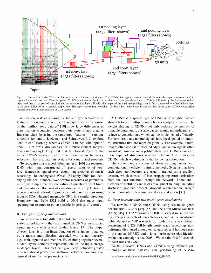
Fig. 1. Illustration of the CDNN architecture we use for our experiments. The CDNN first applies narrow vertical filters to the input sonogram (left) tocapture harmonic structure. Then, it applies 32 different filters in the first convolutional layer (we show only 4). This is followed by the first max-poolinglayer, and then a 2nd pair of convolutional and max-pooling layers. Finally, the output of the final max-pooling layer is fully connected to a final hidden layerof 50 units, followed by a softmax output unit. The input spectrogram contains 100 time slices, which means that the final layer of the CDNN summarisesinformation over a total duration of 2.35 seconds.
classification, instead of using the hidden layer activations asfeatures for a separate classifier. Their experiments in a portionof the “million song dataset” [10] show large differences inclassification accuracies between their systems and a naiveBayesian classifier using the same input features. In a uniquedirection for audio, Dieleman and Schrauwen [19] explore“end-to-end” learning, where a CDNN is trained with input ofabout 3 s of raw audio samples for a music content analysistask (autotagging). They find that the lowest layer of thetrained CDNN appears to learn some filters that are frequencyselective. They evaluate this system for a multilabel problem.
To recognise music mood, Weninger et al. [60] use recurrentDNN with input constructed of several statistics of low-level features computed over second-long excerpts of musicrecordings. Battenberg and Wessel [5] apply DBN for iden-tifying the beat numbers over several measures of percussivemusic, with input features consisting of quantised onset timesand magnitudes. Boulanger-Lewandowski et al. [11] train arecurrent neural network to produce chord classifications usinginput of PCA-whitened magnitude DFT. In a similar direction,Humphrey and Bello [32] build a DNN that maps inputspectrogram features to guitar-specific fingerings of chords.
B. Two types of deep architectures
We now review two different architectures of deep learningsystems, and the way they are trained. A DNN is an artificialneural network with several hidden layers [17]. The outputof each layer is a non-linear function of its inputs, obtainedby a matrix multiplication cascaded with a non-linearity,e.g., tanh, sigmoid and rectifier. By chaining together severalhidden layers, composite representations of the input emergein deeper layers. This fact can give deep networks greaterrepresentational power than shallower networks containing anequivalent number of parameters [7].
A CDNN is a special type of DNN with weights that areshared between multiple points between adjacent layers. Theweight sharing in CDNNs not only reduces the number oftrainable parameters, but also causes matrix multiplications toreduce to convolutions, which can be implemented efficiently.Furthermore, many natural signals have local spatial or tempo-ral structures that are repeated globally. For example, naturalimages often consist of oriented edges; and audio signals oftenconsist of harmonic and repetitive structures. CDNNs can learnthese types of structures very well. Figure 1 illustrates ourCDNN, which we discuss in the following subsection.
The contemporary success of deep learning comes withcomputationally efficient training methods. Systems that havesuch deep architectures are usually trained using gradientdescent, which consists of backpropagating error derivativesfrom the cost function through the network. There are aplethora of useful tips and tricks to augment training, includingstochastic gradient descent, dropout regularisation, weightdecay, momentum, learning rate decay, and so on [37].
C. Deep learning with two music genre benchmarksWe now build DNNs and CDNNs using two music genre
benchmarks: GTZAN [49], [55] and the Latin Music Database(LMD) [45]. GTZAN consists of 100 30-second music record-ing excerpts in each of ten categories, and is the most-usedpublic dataset in MIR research [50]. LMD is a private dataset,consisting of 3,229 full-length music track recordings non-uniformly distributed among ten categories, and has been usedin the annual MIREX audio latin music genre classificationevaluation campaign since 2008.1 We use the first 30 secondsof each track in LMD.
We build several DNNs and CDNNs using different par-titionings of these datasets. One partitioning of GTZAN
we create by randomly selecting 500/250/250 excerpts fortraining/validation/testing. The other partitioning of GTZANis “fault-filtered,” which we construct by hand to include443/197/290 excerpts. This involves removing 70 files includ-ing exact replicas, recording replicas, and distorted files [49],and then dividing the excerpts such that no artist is repeatedacross the training, validation, and test partitions. We partitionLMD in two ways: 1) partitioning by 60/20/20% samplingin each class; 2) a hand-constructed artist-filtered partitioningcontaining approximately the same division of excerpts in eachclass. We retain all 213 replicas in LMD.2
The input to our systems is derived from the short-timeFourier transform (STFT) of a sampled audio signal x [1]:
F(x)[m,u] =
L−1∑l=0
w[l]x[l − uH]e−j2πml/L (1)
where the parameter L defines both the window length and thenumber of frequency bins. We define w as a Hann window oflength L = 1024, which corresponds to a duration of 46msfor recordings sampled at 22050 Hz. The window is hoppedalong x with a stride of H = 512 samples (adjacent windowsoverlap by 50%).
Since audio signals can be of any duration, we define theinput to our systems as a sequence X = (Xn)N−1
n=0 , where thesequence length depends on the input audio’s duration. Wedefine the nth element of the input sequence X to be
Xn ,(∣∣∣F(x)[m,u]
∣∣∣ : m ∈ [0, 512], u ∈ [nT, (n+1)T [)
(2)
where T = 1 for each DNN and T = 100 for each CDNN.Thus, when T = 1, X is a sequence of 513×1 vectors; whenT = 100, X is a sequence of 513× 100 matrices.
A (C)DNN processes each element in this sequence inde-pendently, outputting a sequence P = (Pn)N−1
n=0 from the final(softmax) layer. The output vector Pn ∈ [0, 1]K , ‖Pn‖1 = 1,is the posterior distribution of labels assigned to the nthelement in the input sequence by the network. Therefore, wemay write Pn(i|Xn,Θ) ≡ Pn(i) ∈ [0, 1] where Θ representsthe trainable network parameters, i.e., the set of weights andbiases. We define the confidence of a (C)DNN in a particularlabel k ∈ {1, . . . ,K} for an input sequence X as the sum ofall posteriors, i.e.,
R(k|X,Θ) =1
N
N−1∑n=0
Pn(k|Xn,Θ). (3)
We apply a label to an input sequence X as the one maximis-ing the confidence
y(X,Θ) = arg maxk∈{1,...,K}
R(k|X,Θ). (4)
Paralleling the work in [44], we build DNNs with 3 fullyconnected hidden layers, and either 50 or 500 units per layer.Our CDNN has two convolutional layers (accompanied bymax pooling layers) followed by a fully connected hiddenlayer with 50 units. Figure 1 illustrates the architecture of ourCDNN. Its first convolutional layer contains 32 filters, each
2https://highnoongmt.wordpress.com/2014/02/08/faults in the latin music database
arranged in a rectangular 400 × 4 grid. We choose this longrectangular shape instead of the small square patches typicallyused when training on images based on our knowledge thatmany sounds exhibit strong harmonic structures that span alarge portion of the audible spectrum. The second convolu-tional layer contains 32 filters, each connected in an 8 × 8pattern. Our two pooling neighborhoods are 4 × 4 and havestrides of 2×2. All of our deep learning systems use rectifiedlinear units (ReLUs), and have a softmax unit in the final layer.As is typical, we standardise the (C)DNN inputs by subtractingthe training set mean and dividing by the standard deviationin each of the input dimensions. We perform this with a linearlayer above the input layer of each network. The raw inputsto the network are still Xn.
Also paralleling [44], we build several music classificationsystems treating our DNN as a feature extractor. In this case,we construct a set of features by concatenating the activationsfrom the DNN’s three hidden layers, and aggregating themover 5-second texture windows (hopped by 50%). The ag-gregation summarises the mean and standard deviation of thefeature dimensions over the texture window and may be seenas a form of late-integration of temporal information. We usethis new set of features to train a random forest (RF) classifier[29] with 500 trees. Thus, to classify a music audio recordingx from its set of aggregated features, we use majority votingover all classifications, which is also used in [44].
D. Preliminary evaluation
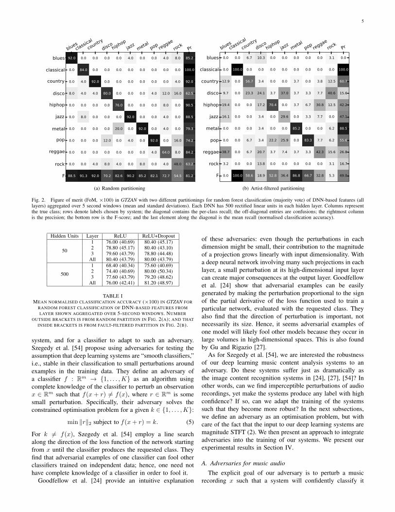
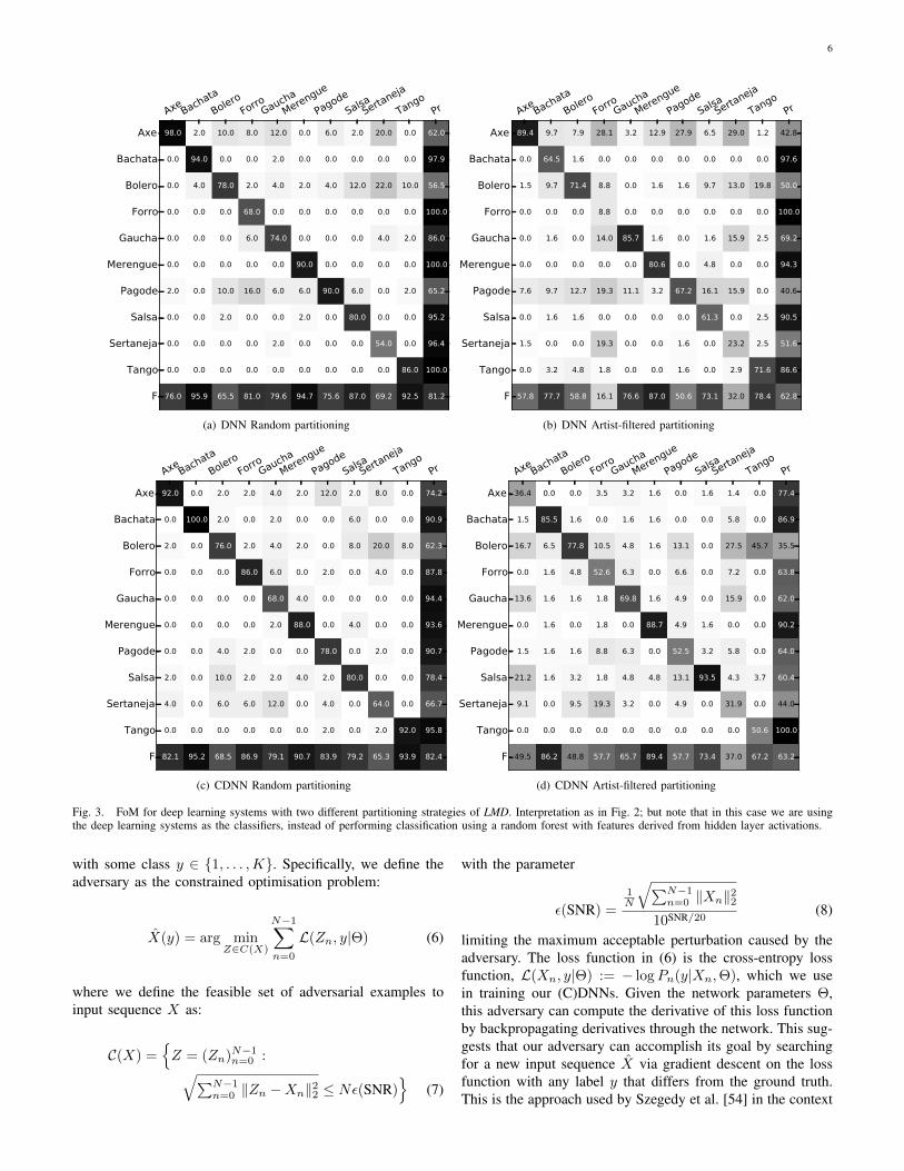
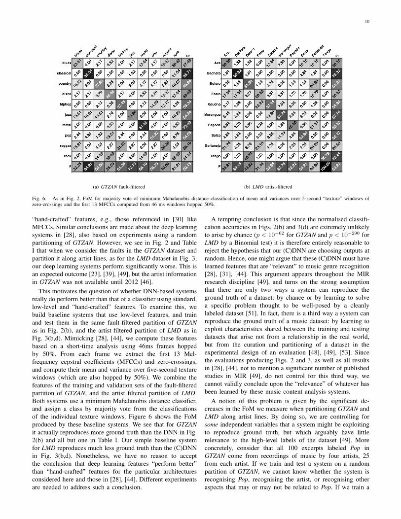
Figure 2 and Table I show the results of RF classificationusing the features produced by the DNN when trained onGTZAN with the two different partitioning strategies; and Fig.3 shows those for the (C)DNNs we train and test in LMD.Across each partition strategy we see significant differencesin performance. The mean recall in each class in Figure 2on the fault-filtered partition is much lower than that onthe random test partition — involving drops higher than 30percentage points in most cases. Table I shows similar dropsin performance that persist over the inclusion of drop-outregularisation. Such significant drops in performance frompartitioning based on artists is not unusual, and has beenstudied before as a bias coming from the experimental design[23], [39], [49]. Partitioning a music genre recognition datasetalong artist lines has been recommended to avoid this bias[23], [39], and is in fact used in several MIREX audioclassification tasks.3 Experiments using GTZAN with fault-filtering partitioning has not been used in many benchmarkexperiments with GTZAN because its artist information hasonly recently been made available [49].
III. ADVERSARIES IN MUSIC CONTENT ANALYSIS
An adversary is an agent that tries to defeat a classificationsystem in order to maximise its gain, e.g., SPAM detection.Dalvi et al. [16] pose this problem as a game between aclassifier and adversary, and analyse the strategies involvedfor an adversary with complete knowledge of the classification
Fig. 2. Figure of merit (FoM, ×100) in GTZAN with two different partitionings for random forest classification (majority vote) of DNN-based features (alllayers) aggregated over 5 second windows (mean and standard deviations). Each DNN has 500 rectified linear units in each hidden layer. Columns representthe true class; rows denote labels chosen by system; the diagonal contains the per-class recall; the off-diagonal entries are confusions; the rightmost columnis the precision; the bottom row is the F-score; and the last element along the diagonal is the mean recall (normalised classification accuracy).
TABLE IMEAN NORMALISED CLASSIFICATION ACCURACY (×100) IN GTZAN FOR
RANDOM FOREST CLASSIFICATION OF DNN-BASED FEATURES FROMLAYER SHOWN AGGREGATED OVER 5-SECOND WINDOWS. NUMBER
OUTSIDE BRACKETS IS FROM RANDOM PARTITION IN FIG. 2(A); AND THATINSIDE BRACKETS IS FROM FAULT-FILTERED PARTITION IN FIG. 2(B).
system, and for a classifier to adapt to such an adversary.Szegedy et al. [54] propose using adversaries for testing theassumption that deep learning systems are “smooth classifiers,”i.e., stable in their classification to small perturbations aroundexamples in the training data. They define an adversary ofa classifier f : Rm → {1, . . . ,K} as an algorithm usingcomplete knowledge of the classifier to perturb an observationx ∈ Rm such that f(x + r) 6= f(x), where r ∈ Rm is somesmall perturbation. Specifically, their adversary solves theconstrained optimisation problem for a given k ∈ {1, . . . ,K}:
min ‖r‖2 subject to f(x+ r) = k. (5)
For k 6= f(x), Szegedy et al. [54] employ a line searchalong the direction of the loss function of the network startingfrom x until the classifier produces the requested class. Theyfind that adversarial examples of one classifier can fool otherclassifiers trained on independent data; hence, one need nothave complete knowledge of a classifier in order to fool it.
Goodfellow et al. [24] provide an intuitive explanation
of these adversaries: even though the perturbations in eachdimension might be small, their contribution to the magnitudeof a projection grows linearly with input dimensionality. Witha deep neural network involving many such projections in eachlayer, a small perturbation at its high-dimensional input layercan create major consequences at the output layer. Goodfellowet al. [24] show that adversarial examples can be easilygenerated by making the perturbation proportional to the signof the partial derivative of the loss function used to train aparticular network, evaluated with the requested class. Theyalso find that the direction of perturbation is important, notnecessarily its size. Hence, it seems adversarial examples ofone model will likely fool other models because they occur inlarge volumes in high-dimensional spaces. This is also foundby Gu and Rigazio [27].
As for Szegedy et al. [54], we are interested the robustnessof our deep learning music content analysis systems to anadversary. Do these systems suffer just as dramatically asthe image content recognition systems in [24], [27], [54]? Inother words, can we find imperceptible perturbations of audiorecordings, yet make the systems produce any label with highconfidence? If so, can we adapt the training of the systemssuch that they become more robust? In the next subsections,we define an adversary as an optimisation problem, but withcare of the fact that the input to our deep learning systems aremagnitude STFT (2). We then present an approach to integrateadversaries into the training of our systems. We present ourexperimental results in Section IV.
A. Adversaries for music audio
The explicit goal of our adversary is to perturb a musicrecording x such that a system will confidently classify it
Fig. 3. FoM for deep learning systems with two different partitioning strategies of LMD. Interpretation as in Fig. 2; but note that in this case we are usingthe deep learning systems as the classifiers, instead of performing classification using a random forest with features derived from hidden layer activations.
with some class y ∈ {1, . . . ,K}. Specifically, we define theadversary as the constrained optimisation problem:
X(y) = arg minZ∈C(X)
N−1∑n=0
L(Zn, y|Θ) (6)
where we define the feasible set of adversarial examples toinput sequence X as:
C(X) ={Z = (Zn)N−1
n=0 :√∑N−1n=0 ‖Zn −Xn‖22 ≤ Nε(SNR)
}(7)
with the parameter
ε(SNR) =
1N
√∑N−1n=0 ‖Xn‖22
10SNR/20(8)
limiting the maximum acceptable perturbation caused by theadversary. The loss function in (6) is the cross-entropy lossfunction, L(Xn, y|Θ) := − logPn(y|Xn,Θ), which we usein training our (C)DNNs. Given the network parameters Θ,this adversary can compute the derivative of this loss functionby backpropagating derivatives through the network. This sug-gests that our adversary can accomplish its goal by searchingfor a new input sequence X via gradient descent on the lossfunction with any label y that differs from the ground truth.This is the approach used by Szegedy et al. [54] in the context
7
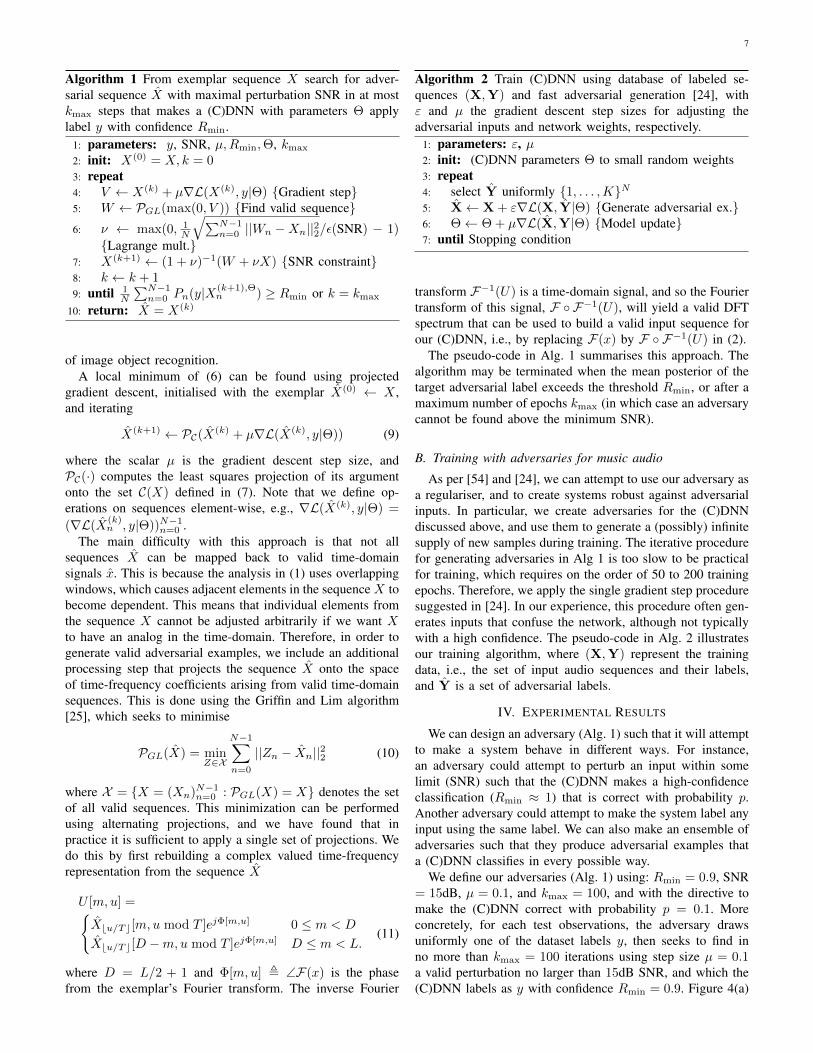
Algorithm 1 From exemplar sequence X search for adver-sarial sequence X with maximal perturbation SNR in at mostkmax steps that makes a (C)DNN with parameters Θ applylabel y with confidence Rmin.
1: parameters: y, SNR, µ,Rmin,Θ, kmax
2: init: X(0) = X, k = 03: repeat4: V ← X(k) + µ∇L(X(k), y|Θ) {Gradient step}5: W ← PGL(max(0, V )) {Find valid sequence}6: ν ← max(0, 1
N
√∑N−1n=0 ||Wn −Xn||22/ε(SNR) − 1)
{Lagrange mult.}7: X(k+1) ← (1 + ν)−1(W + νX) {SNR constraint}8: k ← k + 19: until 1
N
∑N−1n=0 Pn(y|X(k+1),Θ
n ) ≥ Rmin or k = kmax
10: return: X = X(k)
of image object recognition.A local minimum of (6) can be found using projected
gradient descent, initialised with the exemplar X(0) ← X ,and iterating
X(k+1) ← PC(X(k) + µ∇L(X(k), y|Θ)) (9)
where the scalar µ is the gradient descent step size, andPC(·) computes the least squares projection of its argumentonto the set C(X) defined in (7). Note that we define op-erations on sequences element-wise, e.g., ∇L(X(k), y|Θ) =
(∇L(X(k)n , y|Θ))N−1
n=0 .The main difficulty with this approach is that not all
sequences X can be mapped back to valid time-domainsignals x. This is because the analysis in (1) uses overlappingwindows, which causes adjacent elements in the sequence X tobecome dependent. This means that individual elements fromthe sequence X cannot be adjusted arbitrarily if we want Xto have an analog in the time-domain. Therefore, in order togenerate valid adversarial examples, we include an additionalprocessing step that projects the sequence X onto the spaceof time-frequency coefficients arising from valid time-domainsequences. This is done using the Griffin and Lim algorithm[25], which seeks to minimise
PGL(X) = minZ∈X
N−1∑n=0
||Zn − Xn||22 (10)
where X = {X = (Xn)N−1n=0 : PGL(X) = X} denotes the set
of all valid sequences. This minimization can be performedusing alternating projections, and we have found that inpractice it is sufficient to apply a single set of projections. Wedo this by first rebuilding a complex valued time-frequencyrepresentation from the sequence X
U [m,u] ={Xbu/Tc[m,u mod T ]ejΦ[m,u] 0 ≤ m < D
Xbu/Tc[D −m,u mod T ]ejΦ[m,u] D ≤ m < L.(11)
where D = L/2 + 1 and Φ[m,u] , ∠F(x) is the phasefrom the exemplar’s Fourier transform. The inverse Fourier
Algorithm 2 Train (C)DNN using database of labeled se-quences (X,Y) and fast adversarial generation [24], withε and µ the gradient descent step sizes for adjusting theadversarial inputs and network weights, respectively.
1: parameters: ε, µ2: init: (C)DNN parameters Θ to small random weights3: repeat4: select Y uniformly {1, . . . ,K}N5: X← X + ε∇L(X, Y|Θ) {Generate adversarial ex.}6: Θ← Θ + µ∇L(X,Y|Θ) {Model update}7: until Stopping condition
transform F−1(U) is a time-domain signal, and so the Fouriertransform of this signal, F ◦ F−1(U), will yield a valid DFTspectrum that can be used to build a valid input sequence forour (C)DNN, i.e., by replacing F(x) by F ◦ F−1(U) in (2).
The pseudo-code in Alg. 1 summarises this approach. Thealgorithm may be terminated when the mean posterior of thetarget adversarial label exceeds the threshold Rmin, or after amaximum number of epochs kmax (in which case an adversarycannot be found above the minimum SNR).
B. Training with adversaries for music audio
As per [54] and [24], we can attempt to use our adversary asa regulariser, and to create systems robust against adversarialinputs. In particular, we create adversaries for the (C)DNNdiscussed above, and use them to generate a (possibly) infinitesupply of new samples during training. The iterative procedurefor generating adversaries in Alg 1 is too slow to be practicalfor training, which requires on the order of 50 to 200 trainingepochs. Therefore, we apply the single gradient step proceduresuggested in [24]. In our experience, this procedure often gen-erates inputs that confuse the network, although not typicallywith a high confidence. The pseudo-code in Alg. 2 illustratesour training algorithm, where (X,Y) represent the trainingdata, i.e., the set of input audio sequences and their labels,and Y is a set of adversarial labels.
IV. EXPERIMENTAL RESULTS
We can design an adversary (Alg. 1) such that it will attemptto make a system behave in different ways. For instance,an adversary could attempt to perturb an input within somelimit (SNR) such that the (C)DNN makes a high-confidenceclassification (Rmin ≈ 1) that is correct with probability p.Another adversary could attempt to make the system label anyinput using the same label. We can also make an ensemble ofadversaries such that they produce adversarial examples thata (C)DNN classifies in every possible way.
We define our adversaries (Alg. 1) using: Rmin = 0.9, SNR= 15dB, µ = 0.1, and kmax = 100, and with the directive tomake the (C)DNN correct with probability p = 0.1. Moreconcretely, for each test observations, the adversary drawsuniformly one of the dataset labels y, then seeks to find inno more than kmax = 100 iterations using step size µ = 0.1a valid perturbation no larger than 15dB SNR, and which the(C)DNN labels as y with confidence Rmin = 0.9. Figure 4(a)
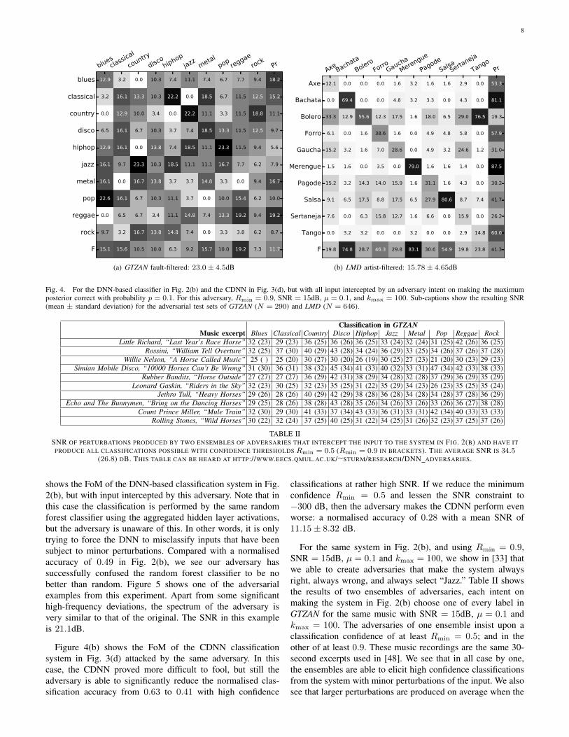
Fig. 4. For the DNN-based classifier in Fig. 2(b) and the CDNN in Fig. 3(d), but with all input intercepted by an adversary intent on making the maximumposterior correct with probability p = 0.1. For this adversary, Rmin = 0.9, SNR = 15dB, µ = 0.1, and kmax = 100. Sub-captions show the resulting SNR(mean ± standard deviation) for the adversarial test sets of GTZAN (N = 290) and LMD (N = 646).
Classification in GTZANMusic excerpt Blues Classical Country Disco Hiphop Jazz Metal Pop Reggae Rock
TABLE IISNR OF PERTURBATIONS PRODUCED BY TWO ENSEMBLES OF ADVERSARIES THAT INTERCEPT THE INPUT TO THE SYSTEM IN FIG. 2(B) AND HAVE IT
PRODUCE ALL CLASSIFICATIONS POSSIBLE WITH CONFIDENCE THRESHOLDS Rmin = 0.5 (Rmin = 0.9 IN BRACKETS). THE AVERAGE SNR IS 34.5(26.8) DB. THIS TABLE CAN BE HEARD AT HTTP://WWW.EECS.QMUL.AC.UK/∼STURM/RESEARCH/DNN ADVERSARIES.
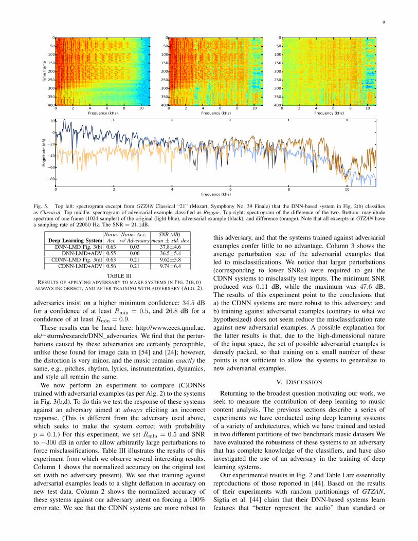
shows the FoM of the DNN-based classification system in Fig.2(b), but with input intercepted by this adversary. Note that inthis case the classification is performed by the same randomforest classifier using the aggregated hidden layer activations,but the adversary is unaware of this. In other words, it is onlytrying to force the DNN to misclassify inputs that have beensubject to minor perturbations. Compared with a normalisedaccuracy of 0.49 in Fig. 2(b), we see our adversary hassuccessfully confused the random forest classifier to be nobetter than random. Figure 5 shows one of the adversarialexamples from this experiment. Apart from some significanthigh-frequency deviations, the spectrum of the adversary isvery similar to that of the original. The SNR in this exampleis 21.1dB.
Figure 4(b) shows the FoM of the CDNN classificationsystem in Fig. 3(d) attacked by the same adversary. In thiscase, the CDNN proved more difficult to fool, but still theadversary is able to significantly reduce the normalised clas-sification accuracy from 0.63 to 0.41 with high confidence
classifications at rather high SNR. If we reduce the minimumconfidence Rmin = 0.5 and lessen the SNR constraint to−300 dB, then the adversary makes the CDNN perform evenworse: a normalised accuracy of 0.28 with a mean SNR of11.15± 8.32 dB.
For the same system in Fig. 2(b), and using Rmin = 0.9,SNR = 15dB, µ = 0.1 and kmax = 100, we show in [33] thatwe able to create adversaries that make the system alwaysright, always wrong, and always select “Jazz.” Table II showsthe results of two ensembles of adversaries, each intent onmaking the system in Fig. 2(b) choose one of every label inGTZAN for the same music with SNR = 15dB, µ = 0.1 andkmax = 100. The adversaries of one ensemble insist upon aclassification confidence of at least Rmin = 0.5; and in theother of at least 0.9. These music recordings are the same 30-second excerpts used in [48]. We see that in all case by one,the ensembles are able to elicit high confidence classificationsfrom the system with minor perturbations of the input. We alsosee that larger perturbations are produced on average when the
Fig. 5. Top left: spectrogram excerpt from GTZAN Classical “21” (Mozart, Symphony No. 39 Finale) that the DNN-based system in Fig. 2(b) classifiesas Classical. Top middle: spectrogram of adversarial example classified as Reggae. Top right: spectrogram of the difference of the two. Bottom: magnitudespectrum of one frame (1024 samples) of the original (light blue), adversarial example (black), and difference (orange). Note that all excerpts in GTZAN havea sampling rate of 22050 Hz. The SNR = 21.1dB.
Norm. Norm. Acc. SNR (dB)Deep Learning System Acc w/ Adversary mean ± std. dev.
TABLE IIIRESULTS OF APPLYING ADVERSARY TO MAKE SYSTEMS IN FIG. 3(B,D)
ALWAYS INCORRECT, AND AFTER TRAINING WITH ADVERSARY (ALG. 2).
adversaries insist on a higher minimum confidence: 34.5 dBfor a confidence of at least Rmin = 0.5, and 26.8 dB for aconfidence of at least Rmin = 0.9.
These results can be heard here: http://www.eecs.qmul.ac.uk/∼sturm/research/DNN adversaries. We find that the pertur-bations caused by these adversaries are certainly perceptible,unlike those found for image data in [54] and [24]; however,the distortion is very minor, and the music remains exactly thesame, e.g., pitches, rhythm, lyrics, instrumentation, dynamics,and style all remain the same.
We now perform an experiment to compare (C)DNNstrained with adversarial examples (as per Alg. 2) to the systemsin Fig. 3(b,d). To do this we test the response of these systemsagainst an adversary aimed at always eliciting an incorrectresponse. (This is different from the adversary used above,which seeks to make the system correct with probabilityp = 0.1.) For this experiment, we set Rmin = 0.5 and SNRto −300 dB in order to allow arbitrarily large perturbations toforce misclassifications. Table III illustrates the results of thisexperiment from which we observe several interesting results.Column 1 shows the normalized accuracy on the original testset (with no adversary present). We see that training againstadversarial examples leads to a slight deflation in accuracy onnew test data. Column 2 shows the normalized accuracy ofthese systems against our adversary intent on forcing a 100%error rate. We see that the CDNN systems are more robust to
this adversary, and that the systems trained against adversarialexamples confer little to no advantage. Column 3 shows theaverage perturbation size of the adversarial examples thatled to misclassifications. We notice that larger perturbations(corresponding to lower SNRs) were required to get theCDNN systems to misclassify test inputs. The minimum SNRproduced was 0.11 dB, while the maximum was 47.6 dB.The results of this experiment point to the conclusions thata) the CDNN systems are more robust to this adversary; andb) training against adversarial examples (contrary to what wehypothesized) does not seem reduce the misclassification rateagainst new adversarial examples. A possible explanation forthe latter results is that, due to the high-dimensional natureof the input space, the set of possible adversarial examples isdensely packed, so that training on a small number of thesepoints is not sufficient to allow the systems to generalize tonew adversarial examples.
V. DISCUSSION
Returning to the broadest question motivating our work, weseek to measure the contribution of deep learning to musiccontent analysis. The previous sections describe a series ofexperiments we have conducted using deep learning systemsof a variety of architectures, which we have trained and testedin two different partitions of two benchmark music datasets Wehave evaluated the robustness of these systems to an adversarythat has complete knowledge of the classifiers, and have alsoinvestigated the use of an adversary in the training of deeplearning systems.
Our experimental results in Fig. 2 and Table I are essentiallyreproductions of those reported in [44]. Based on the resultsof their experiments with random partitionings of GTZAN,Sigtia et al. [44] claim that their DNN-based systems learnfeatures that “better represent the audio” than standard or
Fig. 6. As in Fig. 2, FoM for majority vote of minimum Mahalanobis distance classification of mean and variances over 5-second “texture” windows ofzero-crossings and the first 13 MFCCs computed from 46 ms windows hopped 50%.
“hand-crafted” features, e.g., those referenced in [30] likeMFCCs. Similar conclusions are made about the deep learningsystems in [28], also based on experiments using a randompartitioning of GTZAN. However, we see in Fig. 2 and TableI that when we consider the faults in the GTZAN dataset andpartition it along artist lines, as for the LMD dataset in Fig. 3,our deep learning systems perform significantly worse. This isan expected outcome [23], [39], [49], but the artist informationin GTZAN was not available until 2012 [46].
This motivates the question of whether DNN-based systemsreally do perform better than that of a classifier using standard,low-level and “hand-crafted” features. To examine this, webuild baseline systems that use low-level features, and trainand test them in the same fault-filtered partition of GTZANas in Fig. 2(b), and the artist-filtered partition of LMD as inFig. 3(b,d). Mimicking [28], [44], we compute these featuresbased on a short-time analysis using 46ms frames hoppedby 50%. From each frame we extract the first 13 Mel-frequency cepstral coefficients (MFCCs) and zero-crossings,and compute their mean and variance over five-second texturewindows (which are also hopped by 50%). We combine thefeatures of the training and validation sets of the fault-filteredpartition of GTZAN, and the artist filtered partition of LMD.Both systems use a minimum Mahalanobis distance classifier,and assign a class by majority vote from the classificationsof the individual texture windows. Figure 6 shows the FoMproduced by these baseline systems. We see that for GTZANit actually reproduces more ground truth than the DNN in Fig.2(b) and all but one in Table I. Our simple baseline systemfor LMD reproduces much less ground truth than the (C)DNNin Fig. 3(b,d). Nonetheless, we have no reason to acceptthe conclusion that deep learning features “perform better”than “hand-crafted” features for the particular architecturesconsidered here and those in [28], [44]. Different experimentsare needed to address such a conclusion.
A tempting conclusion is that since the normalised classifi-cation accuracies in Figs. 2(b) and 3(d) are extremely unlikelyto arise by chance (p < 10−62 for GTZAN and p < 10−290 forLMD by a Binomial test) it is therefore entirely reasonable toreject the hypothesis that our (C)DNN are choosing outputs atrandom. Hence, one might argue that these (C)DNN must havelearned features that are “relevant” to music genre recognition[28], [31], [44]. This argument appears throughout the MIRresearch discipline [49], and turns on the strong assumptionthat there are only two ways a system can reproduce theground truth of a dataset: by chance or by learning to solvea specific problem thought to be well-posed by a cleanlylabeled dataset [51]. In fact, there is a third way a system canreproduce the ground truth of a music dataset: by learning toexploit characteristics shared between the training and testingdatasets that arise not from a relationship in the real world,but from the curation and partitioning of a dataset in theexperimental design of an evaluation [48], [49], [53]. Sincethe evaluations producing Figs. 2 and 3, as well as all resultsin [28], [44], not to mention a significant number of publishedstudies in MIR [49], do not control for this third way, wecannot validly conclude upon the “relevance” of whatever hasbeen learned by these music content analysis systems.
A notion of this problem is given by the significant de-creases in the FoM we measure when partitioning GTZAN andLMD along artist lines. By doing so, we are controlling forsome independent variables that a system might be exploitingto reproduce ground truth, but which arguably have littlerelevance to the high-level labels of the dataset [49]. Moreconcretely, consider that all 100 excerpts labeled Pop inGTZAN come from recordings of music by four artists, 25from each artist. If we train and test a system on a randompartition of GTZAN, we cannot know whether the system isrecognising Pop, recognising the artist, or recognising otheraspects that may or may not be related to Pop. If we train a
11
system instead with Pop excerpts by three artists, test with thePop excerpts by the fourth artist, then we might be testingsomething closer to Pop recognition. This all depends ondefining what knowledge is relevant to the problem.
A common retort to these arguments is that a system shouldbe able to reproduce ground truth “by any means.” One therebydefines “relevant knowledge” as any correlations that helps asystem reproduce an amount of dataset ground truth that isinconsistent with chance. However, this can lead to circularreasoning: system X has learned “relevant knowledge” becauseit reproduces Y amount of ground truth; system X reproducesY amount of ground truth because it has learned “relevantknowledge.” It is also deaf to one of the major aims of researchin music content analysis [14]: “to make music, or informationabout music, easier to find.” If a music content analysis systemis describing music in ways that do not align with those ofits users, then its usability is in jeopardy no matter its FoMin benchmark datasets [42], [56]. Finally, this means that theproblem thought to be well-posed by a cleanly labeled datasetcan be many things simultaneously — which leads to theproblem of how to validly compare apples and oranges [51].In other words, why compare systems when they are solvingdifferent problems? This also applies to the comparisons abovewith the FoM in Fig. 6.
While we have no idea whether our (C)DNN systems inFig. 3 are exploiting “irrelevant” characteristics in LMD, ourexperimental results with adversaries in Figs. 4 and 5, andTables II and III, indicate that their decision machinery isincredibly sensitive in very strange ways. Our adversaries areable to fool the high-performing deep learning systems byperturbing their input in minor ways. Auditioning the resultsin Table II show that while the music in each recordingremains exactly the same, and the perturbations are very small,the DNN is nearly always fooled into choosing with highconfidence every class it has supposedly learned. The CDNNis similarly defeated by our adversary; however, it is quitenotable that it requires perturbations of far lower SNR thandoes the DNN. We are currently studying the reasons for this.
Our application of adversaries here is close to the “methodof irrelevant transformations” that we apply in [48], [52],[53] to assess the internal models of music content analysissystems, and to test the hypothesis, “the system is usingrelevant criteria to make its decisions.” In [48], we take abrute force approach whereby we apply random but lineartime-invariant and minor filtering to inputs of systems trainedin three different music recording datasets until their FoMbecomes perfect or random. We also make each system applyevery one of its classes to the same music recordings in TableII.4 In [53], we instead apply subtle pitch-preserving time-stretching of music recordings to fool a deep learning systemtrained in the benchmark music dataset BALLROOM [20].We find that through such a transformation we can make thesystem perform perfectly or no better than random by applyingtempo changes of at most 6% to test dataset recordings. Wefind a similar result for the same kind of deep learning system
4These results can be auditioned here: http://www.eecs.qmul.ac.uk/∼sturm/research/TM expt2/index.html
but trained in LMD [52].Our adversary in Alg. 1 moves instead right to the achilles
heel of a deep learning system, coaxing it to behave in arbitraryways for an input simply by making minor perturbations tothe sampled audio waveform that have no effect on the musiccontent it possesses. We observe in Fig. 5 and auditioningTable II that the low- to mid-frequency content of adversarialexamples differs very little from the original recordings, butfind more significant differences in the high-frequency spectra.This suggests that the distribution of energy in the high-frequency spectrum has significant impact on the decisionmachinery of our (C)DNN. The apparent high relevance ofsuch slight characteristics in proportion to that of the actualmusical content of a music recording does not bode wellfor one of the most important aims of machine learning:generalisation.
As observed by Goodfellow et al. [24] in their deep learningsystems taught to recognise objects in images, the impressiveFoM we measure of our deep learning systems may be merelya colourful “Potemkin village.” Employing an adversary toscratch a little below the surface reveals the FoM to becuriously hollow. A system that appears to be solving acomplex problem but actually is not is what we term a “horse”[48], which is a nod to the famous horse Clever Hans: a realhorse that appeared to be a capable mathematician but wasmerely responding to involuntary cues that went undetectedbecause his public demonstrations had no validity to attest tosuch an ability. Measuring the number of correct answers Hansgives in an uncontrolled environment does not give reasonto conclude he comprehends what he appears to be doing.It is the same with the experiments we perform above withsystems labelling observations in GTZAN and LMD. In fact,Goodfellow et al. [24] come to the same conclusion: “Theexistence of adversarial examples suggests that ... being ableto correctly label the test data does not imply that our modelstruly understand the tasks we have asked them to perform”[24]. This observation is now well-known in MIR [47]–[50],but deserves to be repeated.
VI. CONCLUSION
In this article, we have shown how to adapt the adversaryof Szegedy et al. [54] to work within the context of musiccontent analysis using deep learning. We have shown how ouradversary is effective at fooling deep learning systems of dif-ferent architectures, trained on different benchmark datasets.We find our convolutional networks are more robust againstthis adversary than our deep neural networks. We have alsosought to employ the adversary as part of the training of thesesystems, but find it results in systems that remain as sensitiveto the same adversary.
It is of course not very popular for one to be an “adversary”to research, moving quickly to refute conclusions and breaksystems reported in the literature; however, we insist thatbreaking systems leads ultimately to progress. Considerableinsight can be gained by looking behind the veil of perfor-mance metrics in an attempt to determine the mechanismsby which a system operates, and whether the evaluation is
any valid reflection of the qualities we wish to measure. Suchprobing is necessary if we are truly interested in ascertainingwhat a system has learned to do, what its vulnerabilities mightbe, how it compares to competing systems supposedly solvingthe same problem, and how well we can expect it to performwhen used in real-world applications.
ACKNOWLEDGMENTS
CK and JL were supported in part by the Danish Councilfor Strategic Research of the Danish Agency for ScienceTechnology and Innovation under the CoSound project, casenumber 11-115328. This publication only reflects the authors’views.
REFERENCES
[1] J. B. Allen and L. Rabiner. A unified approach to short-time Fourieranalysis and synthesis. Proc. IEEE, 65(11):1558–1564, Nov. 1977.
[2] J.-J. Aucouturier and F. Pachet. Scaling up music playlist generation.In Multimedia and Expo, 2002. ICME ’02. Proceedings. 2002 IEEEInternational Conference on, volume 1, pages 105–108 vol.1, 2002.
[3] J-.J. Aucouturier and F. Pachet. Improving timbre similarity: How highis the sky? J. of Negative Results in Speech and Audio Sciences, 1(1),2004.
[4] Frederic Bastien, Pascal Lamblin, Razvan Pascanu, James Bergstra,Ian J. Goodfellow, Arnaud Bergeron, Nicolas Bouchard, and YoshuaBengio. Theano: new features and speed improvements. Deep Learningand Unsupervised Feature Learning NIPS 2012 Workshop, 2012.
[5] E. Battenberg and D. Wessel. Analyzing drum patterns using conditionaldeep belief networks. In Proc. ISMIR, 2012.
[6] Y. Bengio, I. Goodfellow, and A. Courville. Deep Learning. MIT Press,2015 (in preparation).
[7] Yoshua Bengio. Learning deep architectures for AI. Foundations andtrends in Machine Learning, 2(1):1–127, 2009.
[8] James Bergstra, Olivier Breuleux, Frederic Bastien, Pascal Lamblin,Razvan Pascanu, Guillaume Desjardins, Joseph Turian, David Warde-Farley, and Yoshua Bengio. Theano: a CPU and GPU math expressioncompiler. In Proceedings of the Python for Scientific ComputingConference (SciPy), June 2010. Oral Presentation.
[9] T. Bertin-Mahieux, D. Eck, and M. Mandel. Automatic tagging of audio:The state-of-the-art. In W. Wang, editor, Machine Audition: Principles,Algorithms and Systems. IGI Publishing, 2010.
[10] T. Bertin-Mahieux, D. P.W. Ellis, B. Whitman, and P. Lamere. Themillion song dataset. In Proc. ISMIR, 2011.
[11] N. Boulanger-Lewandowski, Y. Bengio, and P. Vincent. Audio chordrecognition with recurrent neural networks. In Proc. ISMIR, 2013.
[12] C. J. C. Burges, J. C. Platt, and S. Jana. Distortion discriminant analysisfor audio fingerprinting. IEEE Trans. Speech Audio Process., 11(3):165–174, May 2003.
[13] M. Casey, C. Rhodes, and M. Slaney. Analysis of minimum distancesin high-dimensional musical spaces. IEEE Trans. Audio, Speech, Lang.Process., 16(5):1015–1028, July 2008.
[14] M. Casey, R. Veltkamp, M. Goto, M. Leman, C. Rhodes, and M. Slaney.Content-based music information retrieval: Current directions and futurechallenges. Proc. IEEE, 96(4):668–696, Apr. 2008.
[15] Nick Collins. Computational analysis of musical influence: A musico-logical case study using mir tools. In ISMIR, pages 177–182, 2010.
[16] N. Dalvi, P. Domingos, Mausam, S. Sanghai, and D. Verma. Adversarialclassification. KDD, 2004.
[17] L. Deng and D. Yu. Deep Learning: Methods and Applications. NowPublishers, 2014.
[18] S. Dieleman, P. Brakel, and B. Schrauwen. Audio-based music classifi-cation with a pretrained convolutional network. In Proc. ISMIR, 2011.
[19] S. Dieleman and B. Schrauwen. End-to-end learning for music audio.In Acoustics, Speech and Signal Processing (ICASSP), 2014 IEEEInternational Conference on, pages 6964–6968, May 2014.
[20] S. Dixon, F. Gouyon, and G. Widmer. Towards characterisation of musicvia rhythmic patterns. In Proc. ISMIR, pages 509–517, 2004.
[21] S. Ewert, B. Pardo, M. Muller, and M.D. Plumbley. Score-informedsource separation for musical audio recordings: An overview. SignalProcessing Magazine, IEEE, 31(3):116–124, May 2014.
[22] A. Flexer. A closer look on artist filters for musical genre classification.In Proc. ISMIR, pages 341–344, Sep. 2007.
[23] A. Flexer, D. Schnitzer, M. Gasser, and T. Pohle. Combining featuresreduces hubness in audio similarity. In Proc. Int. Symp. Music Info.Retrieval, 2010.
[24] I. J. Goodfellow, J. Shlens, and C. Szegedy. Explaining and harnessingadversarial examples. In Proc. ICLR, 2015.
[25] Daniel Griffin and Jae S Lim. Signal estimation from modified short-time fourier transform. Acoustics, Speech and Signal Processing, IEEETransactions on, 32(2):236–243, 1984.
[26] Niall Griffith and Peter M Todd. Musical networks: Parallel distributedperception and performance. MIT Press, 1999.
[27] S. Gu and L. Rigazio. Towards Deep Neural Network ArchitecturesRobust to Adversarial Examples. ArXiv e-prints, December 2014.
[28] P. Hamel and D. Eck. Learning features from music audio with deepbelief networks. In Proc. ISMIR, 2010.
[29] T. Hastie, R. Tibshirani, and J. Friedman. The Elements of StatisticalLearning: Data Mining, Inference, and Prediction. Springer-Verlag, 2edition, 2009.
[30] M. Henaff, K. Jarrett, K. Kavukcuoglu, and Y. LeCun. Unsupervisedlearning of sparse features for scalable audio classification. In Proc. Int.Soc. Music Info. Retrieval, Miami, FL, Oct. 2011.
[31] E. J. Humphrey, J. P. Bello, and Y. LeCun. Feature learning and deeparchitectures: New directions for music informatics. J. Intell. Info.Systems, 41(3):461–481, 2013.
[32] E.J. Humphrey and J.P. Bello. From music audio to chord tablature:Teaching deep convolutional networks toplay guitar. In Acoustics,Speech and Signal Processing (ICASSP), 2014 IEEE InternationalConference on, pages 6974–6978, May 2014.
[33] C. Kereliuk, B. L. Sturm, and J. Larsen. Deep learning, audio adver-saries, and music content analysis. In Proc. WASPAA, 2015.
[34] H. Lee, Y. Largman, P. Pham, and A. Y. Ng. Unsupervised feature learn-ing for audio classification using convolutional deep belief networks. InProc. Neural Info. Process. Systems, Vancouver, B.C., Canada, Dec.2009.
[35] T. LH. Li, A. B. Chan, and A. HW. Chun. Automatic musical patternfeature extraction using convolutional neural network. In Proc. Int. Conf.Data Mining and Applications, 2010.
[36] B. Matityaho and M. Furst. Neural network based model for classifica-tion of music type. In Proc. Conv. Electrical and Elect. Eng. in Israel,pages 1–5, Mar. 1995.
[37] G. Montavon, G. B. Orr, and K.-R. Muller, editors. Neural Networks,Tricks of the Trade, Reloaded. Lecture Notes in Computer Science(LNCS 7700). Springer, 2012.
[38] A. Nguyen, J. Yosinski, and J. Clune. Deep neural networks are easilyfooled: High confidence predictions for unrecognizable images. In Proc.NIPS, 2014.
[39] E. Pampalk, A. Flexer, and G. Widmer. Improvements of audio-basedmusic similarity and genre classification. In Proc. Int. Soc. Music Info.Retrieval, pages 628–233, Sep. 2005.
[40] G. Papadopoulos and G. Wiggins. Ai methods for algorithmic compo-sition: A survey, a critical view and future prospects. In Proc. AISBSymposim on Musical Creativity, pages 110–117, 1999.
[41] A. Pikrakis. A deep learning approach to rhythm modeling withapplications. In Proc. Int. Workshop Machine Learning and Music, 2013.
[42] M. Schedl, A. Flexer, and J. Urbano. The neglected user in musicinformation retrieval research. J. Intell. Info. Systems, 41(3):523–539,2013.
[43] D. Schwarz. Concatenative sound synthesis: The early years. J. NewMusic Research, 35(1):3–22, Mar. 2006.
[44] S. Sigtia and S. Dixon. Improved music feature learning with deepneural networks. In Acoustics, Speech and Signal Processing (ICASSP),2014 IEEE International Conference on, pages 6959–6963, May 2014.
[45] C. N. Silla, A. L. Koerich, and C. A. A. Kaestner. The Latin musicdatabase. In Proc. ISMIR, 2008.
[46] B. L. Sturm. An analysis of the GTZAN music genre dataset. In Proc.ACM MIRUM Workshop, pages 7–12, Nara, Japan, Nov. 2012.
[47] B. L. Sturm. Classification accuracy is not enough: On the evaluation ofmusic genre recognition systems. J. Intell. Info. Systems, 41(3):371–406,2013.
[48] B. L. Sturm. A simple method to determine if a music informationretrieval system is a “horse”. IEEE Trans. Multimedia, 16(6):1636–1644, 2014.
[49] B. L. Sturm. The state of the art ten years after a state of the art:Future research in music information retrieval. J. New Music Research,43(2):147–172, 2014.
13
[50] B. L. Sturm. A survey of evaluation in music genre recognition.In A. Nurnberger, S. Stober, B. Larsen, and M. Detyniecki, editors,Adaptive Multimedia Retrieval: Semantics, Context, and Adaptation,volume LNCS 8382, pages 29–66, Oct. 2014.
[51] B. L. Sturm. “horse” inside: Seeking causes of the behaviours ofmusic content analysis systems. ACM Computers in Entertainment, 2015(submitted).
[52] B. L. Sturm, C. Kereliuk, and J. Larsen. ¿ el caballo viejo? latin genrerecognition with deep learning and spectral periodicity. In Proc. Int.Conf. on Mathematics and Computation in Music, 2015.
[53] B. L. Sturm, C. Kereliuk, and A. Pikrakis. A closer look at deep learningneural networks with low-level spectral periodicity features. In Proc. Int.Workshop on Cognitive Info. Process., 2014.
[54] C. Szegedy, W. Zaremba, I. Sutskever, J. Bruna, D. Erhan, I. Goodfellow,and R. Fergus. Intriguing properties of neural networks. In Proc. ICLR,2014.
[55] G. Tzanetakis and P. Cook. Musical genre classification of audio signals.IEEE Trans. Speech Audio Process., 10(5):293–302, July 2002.
[56] J. Urbano, M. Schedl, and X. Serra. Evaluation in music informationretrieval. J. Intell. Info. Systems, 41(3):345–369, Dec. 2013.
[57] A. van den Oord, S. Dieleman, and B. Schrauwen. Deep content-basedmusic recommendation. In Proc. NIPS, 2013.
[58] N. Vempala and F. Russo. Predicting emotion from music audio featuresusing neural networks. In Proc. CMMR, 2012.
[59] A. Wang. An industrial strength audio search algorithm. In Proc. Int.Soc. Music Info. Retrieval, Oct. 2003.
[60] F. Weninger, F. Eyben, and B. Schuller. On-line continuous-time musicmood regression with deep recurrent neural networks. In Acoustics,Speech and Signal Processing (ICASSP), 2014 IEEE InternationalConference on, pages 5412–5416, May 2014.
[61] B. Whitman, G. Flake, and S. Lawrence. Artist detection in music withminnowmatch. Proc. IEEE Workshop on Neural Networks for SignalProcessing, pages 559–568, 2001.
[62] G. A. Wiggins. Semantic gap?? Schemantic schmap!! Methodologicalconsiderations in the scientific study of music. In Proc. IEEE Int. Symp.Mulitmedia, pages 477–482, Dec. 2009.
[63] X. Yang, Q. Chen, S. Zhou, and X. Wang. Deep belief networks forautomatic music genre classification. In Proc. INTERSPEECH, pages2433–2436, 2011.
[64] Y.-H. Yang and H. H. Chen. Music Emotion Recognition. CRC Press,2011.
[65] Chiyuan Zhang, G. Evangelopoulos, S. Voinea, L. Rosasco, and T. Pog-gio. A deep representation for invariance and music classification.In Acoustics, Speech and Signal Processing (ICASSP), 2014 IEEEInternational Conference on, pages 6984–6988, May 2014.