Deep Networks for Image-to-Image Translation with Mux and...

Deep Networks for Image-to-Image Translation

with Mux and Demux Layers

Hanwen Liu1, Pablo Navarrete Michelini1, and Dan Zhu1

BOE Technology Group Co., LTD., No.9 Dize Road, BDA, Beijing, 100176,P.R.China

Abstract. Image processing methods using deep convolutional networkshave achieved great successes on quantitative and qualitative assessmentsin many tasks, such as super–resolution, style transfer and and enhance-ment. Most of these solutions use many layers, many filters and complexarchitectures. It is difficult to implement them on mobile devices, e.g.smart phones, because of the limited resources. Many applications needto deploy these methods on mobile devices. But it is difficult becauseof limited resources. In this paper we present a lightweight end–to–enddeep learning approach for image enhancement. To improve the perfor-mance, we present mux layer and demux layers, which could performup–sampling and down–sampling by shuffling the pixels without losingany information of feature maps. For further higher performance, dense-blocks are used in the models. To ensure the consistency of the outputand input, we use weighted L1 loss to increase PSNR. To improve imagequality, we use adversarial loss, contextual loss and perceptual loss asparts of the objective functions during training. And NIQE is used forvalidation to get the best parameters for perceptual quality. Experimentsshow that, compared to the state–of–the–art, our method could improveboth the quantitative and qualitative assessments, as well as the perfor-mance. With this system, we get the third place in PIRM Enhancement–On–Smartphones Challenge 2018(PIRM–EoS Challenge 2018).

Keywords: Mux layer · Demux layer · Image enhancement · Deep learn-ing

1 Introduction

In recent years, embedded cameras in mobile devices have been improved rapidly,which has brought mobile photographs to a substantially new level. However,because of some limits, such as small size, compact lenses and the lack of specifichardware, the quality of mobile photographs is still falling behind DSLR cameras.

Because of high–aperture optics and larger sensors, DSLR cameras couldcapture photographs with higher quality, color rendition and less noise. Thesephysical differences between DSLR cameras and mobile devices lead to a greatgap, making DSLR cameras quality unattainable for compact mobile devices.

2 H. Liu, P. Navarrete and D. Zhu

There have been many methods that could enhance the mobile photographs,but most of them could only adjust global parameters, such brightness or con-trast. They are usually based on some pre-defined rules to adjust these param-eters. However, image quality is very related to textures and image semantics,which are difficult for classic method to improve.

Mobile devices face two big difficulties to take photographs with similar qual-ity of DSLR cameras. One is to find algorithms that could improve photographswith not only global parameters, but also semantic and perceptual qualities.The second problem is to implement these algorithms on mobile devices, whichmeans that these methods should be lightweight.

First, image processing methods based on deep convolutional networks usu-ally could achieve these targets to improve the quality of images. Several solu-tions for different sub–tasks have solved the first problem about image quality.These methods solve image–to–image translation, targeting at translating im-ages from one domain to another. To ensure the high perceptual quality of out-puts, many of them use some particular metrics to measure image quality andput them as part of the objective functions. The sub–tasks include image superresolution, image deblurring, image dehazing and denoising. However, methodsbased deep learning usually cost large number of resources, such as CPU, GPUand memory, which makes it difficult to implement on mobile devices.

Second, to solve the implementation problem, recent deep learning architec-tures have been used. This includes: MobileNet[15], ShuffleNet[16], MeNet[31]and DPED[3]. All these architectures target devices with limited resources.

The remainder of this paper is structured as follows. In Section 2 we introducesome related works to our research. Section 3 explains the main contributions ofthis paper. Section 4 presents our method in detail, include the architecture andloss functions. Section 5 shows experiment results and analysis. Finally, Section6 concludes this paper.

2 Related Work

Image super resolution aims at restoring an original image form its downscaleversion. In [2], they used a CNN and MSE loss to learn how to map low resolu-tion images to high resolution. This is the first deep learning solutions for singleimage super resolution. Later work proposed deeper and more complex architec-tures, such as[4], [5], [6]. Recently, photo–realistic results with high perceptualquality have been possible to achieve by using a pre–trained VGG network forloss function[1] and adversarial networks[7]. They are known to be efficient atrecovering plausible high–frequency components, that look more realistic at thecost of losing distortion values [29].

Image deblurring and dehazing aim at removing artificially added hazeor blur from the images. Usually, MSE loss is used as a loss function and theproposed CNN architectures consist of three to fifteen convolutional layers[8][9][10], or are bi–channel CNNs[11].

Deep Networks for Image-to-Image translation with Mux and Demux Layers 3

Image denoising similarly targets removal of noise and artifacts from theimages. In[12] the authors presented weighted MSE together with a three–layerCNN, while in[13] it was shown that an eight–layer residual CNN performs betterwhen using a standard MSE.

Image enhancement DPED network[3] presented a novel approach for thephoto enhancement task based on learning a mapping between photos frommobile devices and DSLR camera. The model is trained in an end–to–end fashionwithout any additional supervision or manually adjusted features. Authors ofDPED used a multi–term loss function composed of color, texture and contentterms, allowing an efficient image quality estimation.

Improving performance of deep learning models is always an impor-tant direction in the field of deep learning. Many compact networks are de-signed for mobile or embedded applications. SqueezeNet[14] proposed fire mod-ules, where 1× 1 convolutional layer is first applied to squeeze the width of thenetwork, followed by a layer mixing 3 × 3 and 1 × 1 convolutional kernels toreduce parameter. MobileNet[15] exploited depthwise separable convolutions asits building unit, which decompose a standard convolution into a combination ofa depthwise convolution and a pointwise convolution. ShuffleNet[16] used depth-wise convolutions and pointwise group convolutions into the bottleneck unit[17],and proposed the channel shuffle operation to enable inter–group informationexchange. These networks do not use model compression techniques and so theycan be trained without using large models and the training procedure is veryfast.

Improving image quality Contextual loss[19] was proposed to measurethe similarity between the feature distributions of two images. Contextual lossidentifies similar patches between two images, making it better as a perceptualquality target. Another metric to measure perceptual image quality is the Nat-ural Image Quality Evaluator(NIQE) [21]. NIQE is a completely blind imagequality index based on a collection of statistical features that are known to fol-low a multivariate Gaussian for natural images. It can thus quantify how naturalor real image looks without any reference image, providing a perceptual qualityindex similar to a human evaluations such as MOS.

3 Contributions

To solve the problems mentioned before, there are two research targets. One isto present a novel model to keep high performance, and the other is to proposemethods to ensure the high quality of processed images.

To achieve these targets, we make the following contributions:1. Novel layers with shuffling pixels for up–sampling and down–sampling,

which we call Mux and Demux layers, respectively. Mux layers divide inputfeatures into groups, with each group consisting on four input features. By rear-ranging pixels of every group of four features, the output of the Mux layer doublesthe width and height. Thus, it can be used as up–sampling layer in CNN. Demuxlayer converts input features into 4 times the number of features with half the


width and half the height. So Demux layer can be used as down–sampling layer.Because of the shuffling pixels, the outputs keep all the informations from theinputs, as opposed to to standard pooling and unpooling layers.

2. For high performance, we present new CNN architectures. In the newmodels, Mux layer, Demux layer and DenseNet[18] were combined together.Because no information is lost, input images could be down–sampled directlyinstead of pre–processed with convolutional layers. Feature maps processed byconvolutional layers are always in low resolution, thus leading to high efficiency.Besides, DenseNet is also designed for performance, which used densely skipconnections to reduce the parameters of each convolutional layer.

3. Our loss function adds a weighted L1 cost and a contextual loss to the totalloss function used in DPED method, which can improve the perceptual qualityof output images. For validation, we use the NIQE index to find the model withthe best perceptual quality.

4 Method

Image enhancement is a sub–task of image–to–image translation, which wouldtranslate low quality images to images with high quality. So our target is tolearn a mapping from domain X to domain Y , given training dataset {xi}

Ni=1

where xi ∈ X and {yi}Mi=1 where yi ∈ Y . We denote the data distribution

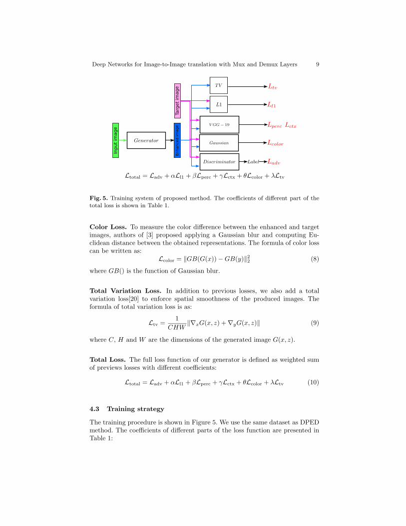
as x ∼ pdata(x) and y ∼ pdata(y). In order to get high frequency details, weadd noise to the input images. So our model is target to learn the mappingfrom the observed images x and noises z to y: G : {x, z} → y. In addition, weintroduce the discriminator D that is trained to distinguish between images {y}and produced images {G(x)}. Finally, the generator G is trained to produceoutputs that cannot be distinguished from “real” images by D. This diagram ofthe system is shown in Figure 5.

To train the model, we use a multi–term loss function which composed ofadversarial loss, weighted loss, perceptual loss, contextual loss, color loss andtotal variation loss.

4.1 Network Architecture

Motivation. Our network architecture is motivated by the well–known designof multi–rate system in digital signal processing [22][23][24]. In multi–rate sys-tems one is interested to analyze an image at different low resolutions withoutlosing information. For one dimensional signals we can take odd and even samples(demuxing) into different filters. If the filters satisfy the so–called Vetterli andVaidyanathan conditions [23] then the original signal can be recovered. Perfectreconstructions is achieved with a system that filters in low resolution and re-combine them into a high–resolution image (muxing). This principle also applieswhen we replace filters by convolutional networks since these can be interpretedas generalized adaptive filters [25]. In prior work we have applied this idea to de-sign image super–resolution systems[26] [27][28] using a so–called MuxOut layer.The later considers only the synthesis stage of multi–rate systems.


Here, we move one step forward to include both the analysis and synthesisstages of multi–rate systems. For image enhancement we need the ”perfect re-construction” property of multi–rate systems to guarantee that we can recoverthe original content. We know that for linear convolutions perfect reconstructionis possible by the Vetterli and Vaidyanathan conditions. When using convolu-tional networks the filters are obtained during the training process, with a lossfunction that can impose the perfect reconstruction target. Our design based onmulti–rate principles guarantee that at least one local minima exists to recoverthe original content. In image enhancement “perfect reconstruction” is not ourfinal target since we want to modify the input image, but it guarantees thatthe architecture would be able to keep all the information needed to solve theproblem when processing at lower resolutions.

Fig. 1. Demux layer and Mux layer.

Mux Layer. [6] proposed an efficient sub–pixel layer called pixel shuffling,which is also based on the theory of multi–rate filters. The pixel shuffling layeris used for up–sampling in the end of convolutional networks to produce threechannels of R, G, and B.

Mux layer is very similar to the pixel shuffling layer, but it can also processfeature maps and produce a varied number of feature maps. So it can be used inthe middle of convolutional networks. Another property of Mux layer is that itcould be used together with Demux layer for perfect reconstruction. As shownin Figure 1, it is the architecture of Mux layer. Mux layer could be used as up–sampling layers in convolutional neural networks, which is based on the theoryof multi–filter. Mux would divide input feature maps into small groups, with


each group consisting of four feature maps. By arranging pixels of every fourfeature maps according to the aforementioned rules, output feature maps wouldbe 2 times higher and 2 time wider than the inputs. And the number of featuremaps is one fourth of the number of inputs.

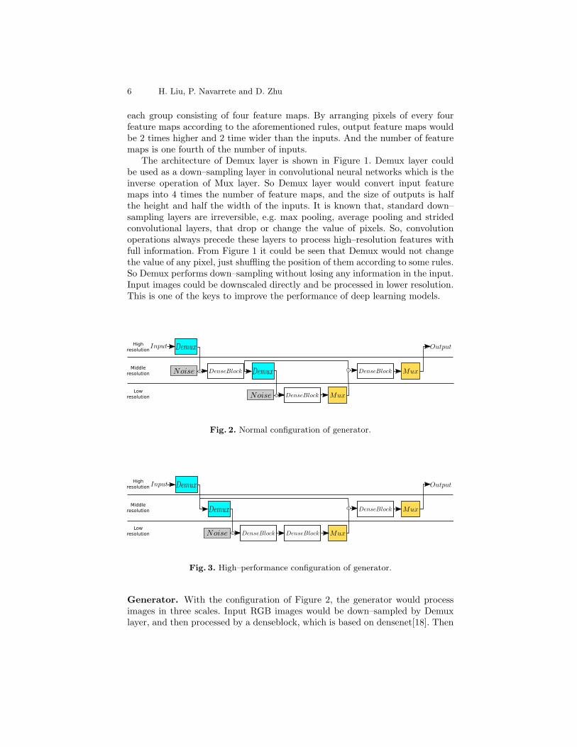
The architecture of Demux layer is shown in Figure 1. Demux layer couldbe used as a down–sampling layer in convolutional neural networks which is theinverse operation of Mux layer. So Demux layer would convert input featuremaps into 4 times the number of feature maps, and the size of outputs is halfthe height and half the width of the inputs. It is known that, standard down–sampling layers are irreversible, e.g. max pooling, average pooling and stridedconvolutional layers, that drop or change the value of pixels. So, convolutionoperations always precede these layers to process high–resolution features withfull information. From Figure 1 it could be seen that Demux would not changethe value of any pixel, just shuffling the position of them according to some rules.So Demux performs down–sampling without losing any information in the input.Input images could be downscaled directly and be processed in lower resolution.This is one of the keys to improve the performance of deep learning models.

C

C

C

High

resolution

Middle

resolution

Low

resolution

Fig. 2. Normal configuration of generator.

C

C

High

resolution

Middle

resolution

Low

resolution

Fig. 3. High–performance configuration of generator.

Generator. With the configuration of Figure 2, the generator would processimages in three scales. Input RGB images would be down–sampled by Demuxlayer, and then processed by a denseblock, which is based on densenet[18]. Then


another Demux and denseblock are used to down–sample the features and pro-cess them. After processing in the third scale, Mux layer is used for up–samplingfollowed by another denseblock. At the end of this model, feature maps are pro-cessed by another Mux layer to get the output RGB image. To generate highfrequency details and get high perceptual quality, noise channels are added tofeature maps after every Demux layers. And we use instance normalization layersafter every 3× 3 convolutional layers to adjust global parameters of the imagesand feature maps.

Another configuration of generator is shown in Figure 3. In this configura-tion, input image is processed by Demux layer two times at the very beginning.So the feature maps would go directly to the third scale. Most of the convolu-tional operations would process feature maps in very small size, thus to reducecomputation complexity and improve performance.

conv

11x

11x4

8

conv

5x5

x128

conv

3x3

x192

conv

3x3

x192

BN

conv

3x3

x128

BN

BN

Fully

Con

nect

ed

Sigm

oid

BN

Fig. 4. Model of discriminator.

Discriminator. Figure 4 shows the architecture of the discriminator, which isthe same as in DPED[3] system. The discriminator consists of five convolutionallayers, each followed by a LeakyReLU activation function and batch normal-ization. The first, second and fifth convolutional layers are strided with a stepsize of 4, 2, and 2, respectively. A sigmoid activation function is applied to theoutput of the last fully connected layer containing 1024 neurons to output theprobability that the input image belongs to the target domain.

4.2 Loss Function

Adversarial Loss. For image enhancement, important differences between in-put images and target images are the brightness, contrast, and texture qualities.We build a generative adversarial network to learn the mapping between inputand target domains. The discriminator observes both generated images (fake)and target images (real), and its goal is to predict whether the input image is realor not. It is trained to minimize a cross–entropy loss function. The adversarialloss for generator is defined as a standard GAN[30]:

Ladv = −∑

i

logD(G(x, z), y) (1)

where G and D denote the generator and discriminator networks, respectively.


Weighted L1 Loss. In order to get close to the DSLR image we applied aweighted L1 loss during training. We calculate the L1 loss of each channel (R,G, and B) between outputs and reference DSLR images, and then combine themtogether with different weights, which are taken from the YUV color conversion.The formula for weighted L1 loss is:

Ll1 = 0.299×‖r(G(x))−r(y)‖1+0.587×‖g(G(x))−g(y)‖1+0.114×‖b(G(x))−b(y)‖1 ,

(2)where r(), g() and b() are the operations to get the R, G, and B channels fromone image, respectively.

Perceptual Loss. Inspired by [1], [7] and [3], we also define our perceptual lossbased on the feature maps extracted by the pre–trained VGG network to measurehigh–level perceptual and semantic differences between images. Let φj(x) be theoutputs of the j–th layer of the pre–trained VGG network φ when processingimage x. If j–th is a convolutional layer, φj(x) would be a feature map of shapeCj×Hj×Wj . Then the perceptual loss of the generator is the Euclidean distancebetween feature representations:

Lperc =1

CjHjWj

[||φj(y)− φj(G(x, z))||2] . (3)

As demonstrated in [1], images reconstructed from the high–layers features tendto preserve the content and overall spatial structure, and not the color, texture,and exact shapes. Using perceptual loss for our image transformation networkencourages the output images to be perceptually similar to the input images,but does not force them to match exactly.

Contextual Loss. Authors of [19] proposed a novel contextual loss that couldbe effective for many image transformation tasks. The contextual loss is definedas below:

CX(x, y) =1

N

∑

j

maxi

CXij , (4)

where CXij is the similarity between features xi and yj , which is defined as:

wij = exp1−

dij

mink di,k+ǫ

h(5)

CXij =wij∑k wik

(6)

where dij is the Cosine distance between xi and yj , ǫ is a fixed value of 0.00001,h > 0 is a band–width parameters.

The final contextual loss function is as:

Lctx = − log(CX(φj(G(x, z)), φj(y))) (7)


Input

image

Enhanced im

age

Targ

et

image

Fig. 5. Training system of proposed method. The coefficients of different part of thetotal loss is shown in Table 1.

Color Loss. To measure the color difference between the enhanced and targetimages, authors of [3] proposed applying a Gaussian blur and computing Eu-clidean distance between the obtained representations. The formula of color losscan be written as:

Lcolor = ‖GB(G(x))−GB(y)‖22 (8)

where GB() is the function of Gaussian blur.

Total Variation Loss. In addition to previous losses, we also add a totalvariation loss[20] to enforce spatial smoothness of the produced images. Theformula of total variation loss is as:

Ltv =1

CHW‖∇xG(x, z) +∇yG(x, z)‖ (9)

where C, H and W are the dimensions of the generated image G(x, z).

Total Loss. The full loss function of our generator is defined as weighted sumof previews losses with different coefficients:

Ltotal = Ladv + αLl1 + βLperc + γLctx + θLcolor + λLtv (10)

4.3 Training strategy

The training procedure is shown in Figure 5. We use the same dataset as DPEDmethod. The coefficients of different parts of the loss function are presented inTable 1:


Table 1. Coefficients of parts of total loss in Formula10 during the experiments.

Parameter α β γ θ λ

Value 5000 10 10 0.5 2000

During the training, we perform validation to avoid over–fitting. For distor-tion quality, we use PSNR and SSIM between the enhanced images and DSLRimages to evaluate the model.

Besides the distortion quality and loss function, we also use NIQE as one ofthe metrics to evaluate the models. For the PIRM-EoS the evaluation considersdifferent aspects. The evaluation formula measures a distortion index (PSNR),perceptual quality (MS-SSIM during validation and MOS for final evaluation),and running time on different devices. From this, MOS score is the most unpre-dictable during training and validation because we cannot reproduce the opinionof people. To approximate the MOS scores we use a linear mapping of the NIQEindex that is know to be linearly correlated to MOS values. Thus, we couldestimate the scores that would be calculated in the test phase of the challenge.

5 Experiments

We use the generator in Figure 2 and Figure 3 for image enhancement. Using thesame test datasets as DPED[3], we compare our method against several solutionsthat are very relevant to the task. To evaluate the performance, we calculate therunning–time of each method while processing images of size 1280× 720.

5.1 Baselines

Apple Photo Enhancer(APE) is a commercial product known to generateone of the best visual results, while the algorithm is unpublished. The method istriggered using automatic Enhance function from the Photos APP. It performsimage improvement without taking any parameters.

SRCNN[2] is a fundamental baseline super–resolution method, thus addressinga task related to end–to–end image–to–image translation. Hence we chose it asa baseline to compare to. The method relies on a standard three–layer CNNand MSE loss function and maps from low resolution / corrupted images to therestored image.

Johnson et al.[1] could get high quality outputs in photo–realistic super res-olution and style transferring tasks. The method is based on a deep residualnetwork that is trained to minimize a VGG–based loss function.

DPED.[3] is one of the state of the art in image enhancement. A similar lossfunction to our method is used for the training to minimize the adversarial loss,perceptual loss, color loss and total variation loss.


ResNet.[17] is an important baseline in the field of classification and imageprocessing. Denseblocks are widely used in deep convolutional networks. In theexperiments, we use two configurations of ResNet, ResNet–8–32 and ResNet–12–64.

5.2 Evaluations

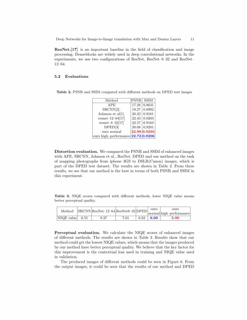
Table 2. PSNR and SSIM compared with different methods on DPED test images

Method PSNR SSIM

APE 17.28 0.8631SRCNN[2]. 19.27 0.8992

Johnson et al[1]. 20.32 0.9161resnet–12–64[17] 22.43 0.9203resnet–8–32[17] 22.57 0.9163

DPED[3] 20.08 0.9201ours normal 22.98 0.9235

ours high–performance 22.73 0.9206

Distortion evaluation. We compared the PSNR and SSIM of enhanced imageswith APE, SRCNN, Johnson et al., ResNet, DPED and our method on the taskof mapping photographs from iphone 3GS to DSLR(Canon) images, which ispart of the DPED test dataset. The results are shown in Table 2. From theseresults, we see that our method is the best in terms of both PSNR and SSIM inthis experiment.

Table 3. NIQE scores compared with different methods, lower NIQE value meansbetter perceptual quality.

Method SRCNN ResNet–12–64 ResNet8–32 DPEDours

normalours

high–performance

NIQE value 6.55 9.37 7.61 6.82 6.00 5.90

Perceptual evaluation. We calculate the NIQE scores of enhanced imagesof different methods. The results are shown in Table 3. Results show that ourmethod could get the lowest NIQE values, which means that the images producedby our method have better perceptual quality. We believe that the key factor forthis improvement is the contextual loss used in training and NIQE value usedin validation.

The produced images of different methods could be seen in Figure 6. Fromthe output images, it could be seen that the results of our method and DPED


Fig. 6. Results comparison of different methods: (a)original iPhone photo,(b)APE,(c)Dong et al[2]. (d)Johnson et al[1].(e)DPED[3], (f)resnet–8–32, (g)our model in nor-mal configuration, (h)our model in high–performance configuration, (i)DSLR image.

are closer to the DSLR image than other methods. We observe, for example, thatDPED increases the brightness excessively in this experiment. The brightness isvisibly stronger than DSLR image. Our method could balance the contrast andartificial details better than other methods.

Performance evaluation. We run this experiment to measure the processingtime of our method and other methods with input image resolution 1280× 720.Table 4 shows that our method shows a significant advantage in processingspeed. It is the Mux and Demux layers that bring this advantage, because theconvolutional operations do now need to process feature maps in large size.

Ablation study. We did the ablation study of the normal configuration genera-tor by removing every part of loss function to find the effect of each loss. Resultsare shown in Table 5. We can get the highest PSNR and SSIM with full losses.When contextual loss was removed the NIQE increased obviously, which means


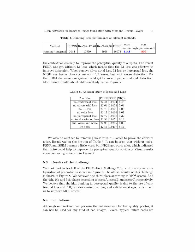
Table 4. Running–time performance of different methods.

Method SRCNN ResNet–12–64 ResNet8–32 DPEDours

normalours

high–performance

running time(ms) 2044 12539 3928 16072 1148 806

the contextual loss help to improve the perceptual quality of outputs. The lowestPSNR was got without L1 loss, which means that the L1 loss was effective toimprove distortion. When remove adversarial loss, L1 loss or perceptual loss, theNIQE was better than system with full losses, but with worse distortion. Forthe PIRM challenge, our system could get balance of perceptual and distortion.More visual results about ablation study are in Figure 7

Table 5. Ablation study of losses and noise

Condition PSNR SSIM NIQE

no contextual loss 22.44 0.9114 6.43no adversarial loss 22.64 0.9173 5.64

no L1 loss 21.79 0.9121 5.08no color loss 22.17 0.9166 6.07

no perceptual loss 22.72 0.9158 5.32no total variation loss 22.53 0.9171 6.13

full losses and noise 22.98 0.9235 6.00

no noise 22.84 0.9207 6.87

We also do another by removing noise with full losses to prove the effect ofnoise. Result was in the bottom of Table 5. It can be seen that without noise,PSNR and SSIM became a little worse but NIQE got worse a lot, which indicatedthat noise could help to improve the perceptual quality obviously. Visual resultsabout removing noise are in Figure 7

5.3 Results of the challenge

We took part in track B of the PIRM–EoS Challenge 2018 with the normal con-figuration of generator as shown in Figure 2. The official results of this challengeis shown in Figure 8. We achieved the third place according to MOS scores. Andthe 4th, 4th and 5th places according to scoreA, scoreB and scoreC, respectively.We believe that the high ranking in perceptual quality is due to the use of con-textual loss and NIQE index during training and validation stages, which helpus to improve MOS scores.

5.4 Limitations

Although our method can perform the enhancement for low quality photos, itcan not be used for any kind of bad images. Several typical failure cases are


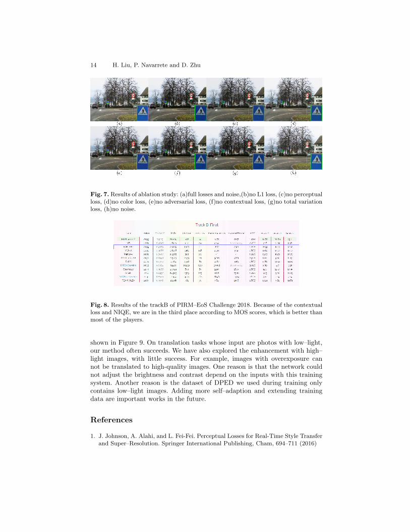
Fig. 7. Results of ablation study: (a)full losses and noise,(b)no L1 loss, (c)no perceptualloss, (d)no color loss, (e)no adversarial loss, (f)no contextual loss, (g)no total variationloss, (h)no noise.

Fig. 8. Results of the trackB of PIRM–EoS Challenge 2018. Because of the contextualloss and NIQE, we are in the third place according to MOS scores, which is better thanmost of the players.

shown in Figure 9. On translation tasks whose input are photos with low–light,our method often succeeds. We have also explored the enhancement with high–light images, with little success. For example, images with overexposure cannot be translated to high-quality images. One reason is that the network couldnot adjust the brightness and contrast depend on the inputs with this trainingsystem. Another reason is the dataset of DPED we used during training onlycontains low–light images. Adding more self–adaption and extending trainingdata are important works in the future.

References

1. J. Johnson, A. Alahi, and L. Fei-Fei. Perceptual Losses for Real-Time Style Transferand Super–Resolution. Springer International Publishing, Cham, 694–711 (2016)


Fig. 9. Failure examples of our methods.Top: input images. Bottom: output images.

2. C. Dong, C. C. Loy, K. He, and X. Tang. Learning a Deep Convolutional Network forImage Super–Resolution. Springer International Publishing, Cham, 184–199 (2014)

3. A. Ignatov, N. Kobyshev, K. Vanhoey, R. Timofte and L. v. Gool. DSLR-QualityPhotos on Mobile Devices with Deep Convolutional Networks. Proceedings of theIEEE international conference on computer vision(2017)

4. J. Kim, J. K. Lee and K. M. Lee. Accurate image super resolution using verydeep convolutional networks. IEEE Conference on Computer Vision and PatternRecognition, 1646–1654(2016)

5. X. Mao, C. Shen, and Y. B. Yang. Image restoration using very deep convolutionalencoder-decoder networks with symmetric skip connections. Advances in neural in-formation processing system 29, 2802–2810(2016)

6. W. Shi, J. Caballero, F. Huszar, J. Totz, A. P. Aitken, R. Bishop, D. Rueckertand Z. Wang. Real–time single image and video super–resolution using an efficientsub–pixel convolutional nerual networks. IEEE Conference on Computer Vision andPattern Recognition,(2016)

7. C. Ledig, L. Theis, F. Huszar, J. Caballero, A. Cunningham, A. Acosta, A. Aitken,A. Tejani, J. Totz, Z. Wang and W. Shi. Photo–realistic single image super–resolution using a generative adversarial network. IEEE Conference on ComputerVision and Pattern Recognition,(2017)

8. B. Cai, X. Xu, K. Jia, C. Qing and D. Tao. Dehazenet: An end–to–end system forsingle image haze removal. IEEE Transactions on Image Processing, 25(11):5287–5298, (2016)

9. M. Hradis, J. Kotera, P. Zemcik and F. Sroubek. Convolutional neural networksfor direct text deblurring. Proceedings of BMVV 2015. The British Machine VisionAssociation and Society for Pattern Recognition. (2015)

10. Z. Ling, G. Fan, Y. Wang, and X. Lu. Learning deep transmission network forsingle image dehazing. IEEE Conference on Computer Vision and Pattern Recog-nition,(2016)

11. W. Ren. S. Liu, H. Zhang, J. Pan, X. Cao, and M. H. Yang. Single image dehazingvia multi-scale convolutional neural networks. Springer International Publishing,Cham 154–169, (2016)

12. X. Zhang and R. Wu. Fast depth image denoising and enhancement using a deepconvolutional network. IEEE International Conference on Acoustics, Speech andSingnal Processing, 2499–2503, (2016)

13. P. Svoboda, M. Hradis, D. Barina, and P. Zemcik. Compression artifacts removalusing convolutional neural networks. CoRR, sbs,1605.00366 (2016)


14. F. N. Iandola, S. Han, M. W. Moskewicz, K. Ashraf, W. J. Dally, and K. Keutzer.Squeezenet: Alexnet-level accuracy with 50x fewer parameters and ¡ 0.5 mb modelsize. arXiv preprint arXiv:1602.07360,(2016).

15. A. G. Howard, M. Zhu, B. Chen, D. Kalenichenko, W. Wang, T. Weyand, M.Andreetto, and H. Adam. Mobilenets: Efficient convolutional neural networks formobile vision applications. arXiv preprint arXiv:1704.04861, (2017).

16. X. Zhang, X. Zhou, M. Lin, and J. Sun. Shufflenet: An extremely efficient convo-lutional neural network for mobile devices. arXiv preprint arXiv:1707.01083, (2017)

17. K. He, X. Zhang, S. Ren, and J. Sun. Deep residual learning for image recogni-tion. Proceedings of the IEEE conference on computer vision and pattern recogni-tion,770778, (2016).

18. G. Huang, Z. Liu, and L. V. D. Maaten. Densely connected convolutional networks.IEEE Conference on Computer Vision and Pattern Recognition,(2017)

19. R. Mechrez, I. Talmi, and L. Z. Manor. The contextual loss for image transforma-tion with non aligned data. arXiv preprint arXiv:1803.02077, (2018)

20. H. A. Aly and E. Dubois. Image up-sampling using totalvariation regulariza-tion with a new observation model. IEEE Transactions on Image Processing,14(10):16471659, Oct 2005

21. A. Mittal, R. Soundararajan, A. C. Bovik. Making a ”completely blind” imagequality analyzer. IEEE Signal Processing Letters, 20(3), 209-212, (2013)

22. J.G. Proakis and D.G. Manolakis. Digital Signal Processing. Prentice Hall inter-national editions. Pearson Prentice Hall, (2007)

23. P. P. Vaidyanathan. Multirate Systems And Filter Banks, Prentice Hall, EnglewoodCliffs, (1993)

24. S. Mallat. A Wavelet Tour of Signal Processing, Academic Press, (1998).25. P. Navarrete and H. Liu. Convolutional networks with muxout layers as multi-rate

systems for image upscaling. CoRR, abs/1705.07772, (2017)26. P. Navarrete, L. Zhang, and J. He. Upscaling with deep convolutional networks

and muxout layers. In GPU Technology Conference 2016, Poster Session, San Jose,CA, USA, May (2016)

27. P. Navarrete and H. Liu. Upscaling beyond superresolution using a novel deeplearning system. GPU Technology Conference, March (2017)

28. R. Timofte, S. Gu, J. Wu, L. Van Gool, L. Zhang, M.-H. Yang, M. Harris, G.Shakhnarovich, N. Ukita, et al. NTIRE 2018 Challenge on Single Image Super-Resolution: Methods and Results. In The IEEE Conference on Computer Visionand Pattern Recognition (CVPR) Workshops , June (2018)

29. Blau, Y., Michaeli, T.: The perception-distortion tradeoff. In: The IEEE Confer-ence on Computer Vision and Pattern Recognition (CVPR) (June 2018)

30. I. Goodfellow, J. Pouget-Abadie, M. Mirza, et al. Generative Adversarial Nets.NIPS, (2014).

31. Z. Qin, Z. Zhang, S. Zhang, H. Yu, and Y. Peng. Merging and evolution: im-proving convolutional neural networks for mobile applications. arXiv preprintarXiv:0803.09127, (2018)

32. H. Liu, P. Navarrete and D. Zhu. Arsty-GAN: a style transfer system with improvedquality, diversity and performance. International Conference on Pattern Recogni-tion,(2018)

Date post:	12-Feb-2020
Category:	Documents
Upload:	others
View:	18 times
Download:	0 times

Deep Networks for Image-to-Image Translation with Mux and...

Documents