Deep Sets

Anonymous Author(s)AffiliationAddressemail

Abstract

We study the problem of designing models for machine learning tasks defined on1

sets. In contrast to traditional approach of operating on fixed dimensional vectors,2

we consider objective functions defined on sets and are invariant to permutations.3

Such problems are widespread, ranging from estimation of population statistics [1],4

to anomaly detection in piezometer data of embankment dams [2], to cosmology [3,5

4]. Our main theorem characterizes the permutation invariant functions and provides6

a family of functions to which any permutation invariant objective function must7

belong. This family of functions has a special structure which enables us to design8

a deep network architecture that can operate on sets and which can be deployed on9

a variety of scenarios including both unsupervised and supervised learning tasks.10

We also derive the necessary and sufficient conditions for permutation equivariance11

in deep models. We demonstrate the applicability of our method on population12

statistic estimation, point cloud classification, set expansion, and outlier detection.13

1 Introduction14

A typical machine learning algorithm, like regression or classification, is designed for fixed-sized15

dimensional data instances. Their extensions to handle the case when the inputs or outputs are16

permutation invariant sets rather than fixed dimensional vectors is not trivial and researchers have17

only recently started to investigate them [5, 6, 7, 8]. In this paper, we present a generic framework to18

deal with the setting where input and possibly output instances in a machine learning task are sets.19

Similarly to fixed dimensional data instances, we can characterize two learning paradigms in case20

of sets. In supervised learning, we have an output label for a set that is invariant or equivariant to21

the permutation of set elements. Examples include tasks like estimation of population statistics [1],22

where applications range from giga-scale cosmology [3, 4] to nano-scale quantum chemistry [9].23

Next, there can be the unsupervised setting, where the “set” structure needs to be learned, e.g. by24

leveraging the homophily/heterophily tendencies within sets. An example is the task of set expansion25

(a.k.a. audience expansion), where given a set of objects that are similar to each other (e.g. set of26

words {lion, tiger, leopard}), our goal is to find new objects from a large pool of candidates such27

that the selected new objects are similar to the query set (e.g. find words like jaguar or cheetah28

among all English words). This is a standard problem in similarity search and metric learning, and29

a typical application is to find new image tags given a small set of possible tags. Likewise, in field30

of computational advertisement, given a set of high-value customers, the goal would be to find31

similar people. This is an important problem in many scientific applications, e.g. given a small set of32

interesting celestial objects, astrophysicists might want to find similar ones in large sky surveys.33

Main contributions. In this paper, i) we propose a fundamental architecture to deal with sets as34

inputs and show that the properties of this architecture are both necessary and sufficient (Sec. 2).35

ii) We extend this architecture to allow for conditioning on arbitrary objects, and iii) based on36

this architecture we develop a deep network that can operate on sets with possibly different sizes37

(Sec. 3). We show that a simple parameter-sharing scheme enables a general treatment of sets within38

supervised and semi-supervised settings. iv) We demonstrate the applicability of our framework39

algorithm through various problems (Sec. 4).40

Submitted to 31st Conference on Neural Information Processing Systems (NIPS 2017). Do not distribute.

2 Permutation Invariance and Equivariance41

2.1 Problem Definition42

A function f transforms its domain X into its range Y . Usually, the input domain is a vector space43

Rd and the output response range is either a discrete space, e.g. {0, 1} in case of classification, or a44

continuous space R in case of regression. Now, if the input is a set X = {x1, . . . , xM}, xm ∈ X, i.e.,45

the input domain is the power set X = 2X, then we would like the response of the function not to be46

“indifferent” to the ordering of the elements in the set. In other words,47

Property 1 A function f : 2X → Y acting on sets must be permutation invariant to the order of48

objects in the set, i.e. for any permutation σ : f({x1, ..., xm}) = f({xσ(1), ..., xσ(M)}).49

In the supervised setting, N examples of of X(1), ..., X(N) as well as their labels y(1), ..., y(N) and50

the task would be to classify/regress (with variable number of predictors) while being permutation51

invariant w.r.t predictors. Under unsupervised setting, the task would be to assign high scores to52

valid sets and low scores to improbable sets. Such score can be used for set expansion tasks, such as53

image tagging or audience expansion in field of computational advertisement. In transductive setting,54

each instance x(n)m has an associated labeled y(n)

m . Then, the objective would be instead to learn55

a permutation equivariant function f : XM → YM that upon permutation of the input instances56

permutes the output labels, i.e. for any permutation σ:57

f([xσ(1), . . . , xσ(M)]) = [fσ(1)(x), . . . , fσ(M)(x)] (1)58 2.2 Structure59

We want to study the structure of functions on set. Their study in total generality is extremely difficult,60

so we analyze case-by-case. Let us begin by analyzing the invariant case when X is a countable set61

and Y = R, then the next theorem characterizes its structure.62

Theorem 2 A function f(X) operating on a set X having elements from a countable universe, is a63

valid set function, i.e., invariant to the permutation of instances in X , iff it can be decomposed in the64

form ρ(∑

x∈X φ(x)), for suitable transformations φ and ρ.65

The extension to case when X is uncountable, like X = R, we could only prove that ρ(∑

x∈X φ(x))

66

is a universal approximator. The proofs and difficulty in handling the uncountable case is discussed67

in Appendix A. However, we still conjecture that exact equality holds.68

Next, we analyze the equivariant case when X = Y = R and f is restricted to be a neural network69

layer. The standard neural network layer is represented as fΘ(x) = σ(Θx) where Θ ∈ RM×M is the70

weight vector and σ : R→ R is a nonlinearity such as sigmoid function. The following lemma states71

the necessary and sufficient conditions for permutation-equivariance in this type of function.72

Lemma 3 The function fΘ : RM → RM defined above is permutation equivariant iff all the off-73

diagonal elements of Θ are tied together and all the diagonal elements are equal as well. That is,74

75Θ = λI + γ (11T) λ, γ ∈ R 1 = [1, . . . , 1]T ∈ RN I ∈ RN×N is the identity matrix

This result can be easily extended to higher dimensions, i.e., when X = Rd.76

2.3 Related Results77

The general form of Theorem 2 is closely related with important results in different domains. Here,78

we quickly review some of these connections.79

de Finetti theorem. A related concept is that of an exchangeable model in Bayesian statistics, It is80

backed by deFinetti’s theorem which states that81

p(x|α) =

∫dθ

[m∏i=1

p(xi|θ)

]p(θ|α). (2)

To see that this fits into our result, let us consider exponential families with conjugate priors, where82

we can analytically calculate the integral of (2). In this special case p(x|θ) = exp (〈φ(x), θ〉 − g(θ))83

and p(θ|α,M0) = exp (〈θ, α〉 −M0g(θ)− h(α,M0)). Now if we marginalize out θ, we get a form84

which looks exactly like the one in Theorem 285

p(x|α) = exp

(h

(α+

∑m

φ(xm),M0 +M

)− h(α,M0)

)(3)

2

Representer theorem and kernel machines. Support distribution machines use f(p) =86 ∑i αiyiK(pi, p) + b as the prediction function [8, 10], where pi, p are distributions and αi, b ∈ R.87

In practice the pi, p distributions are never given to us explicitly, usually only i.i.d. sample sets are88

available from these distributions, and therefore we need to estimate kernel K(p, q) using these89

samples. A popular approach is to use K̂(p, q) = 1MM ′

∑i,j k(xi, yj), where k is another kernel90

operating on the samples {xi}Mi=1 ∼ p and {yj}M′

j=1 ∼ q. Now, these prediction functions can be seen91

fitting into the structure of our Theorem.92

Spectral methods. A consequence of the polynomial decomposition is that spectral methods [11]93

can be viewed as a special case of the mapping ρ ◦ φ(X): in that case one can compute polynomials,94

usually only up to a relatively low degree (such as k = 3), to perform inference about statistical95

properties of the distribution. The statistics are exchangeable in the data, hence they could be96

represented by the above map.97

3 Deep Sets98

3.1 Architecture99

Invariant model. The structure of permutation invariant functions in Theorem 2 hints at a general100

strategy for inference over sets of objects, which we call Deep Sets. Replacing φ and ρ by universal101

approximators leaves matters unchanged, since, in particular, φ and ρ can be used to approximate102

arbitrary polynomials. Then, it remains to learn these approximators, yielding in the following model:103

104 • Each instance xm is transformed (possibly by several layers) into some representation φ(xm).105

• The representations φ(xm) are added up and the output is processed using the ρ network in the106

same manner as in any deep network (e.g. fully connected layers, nonlinearities, etc).107

• Optionally: If we have additional meta-information z, then the above mentioned networks could be108

conditioned to obtain the conditioning mapping φ(xm|z).109

In other words, the key is to add up all representations and then apply nonlinear transformations.110

Equivariant model. Our goal is to design neural network layers that are equivariant to the permuta-111

tions of elements in the input x. Based on Lemma 3, a neural network layer fΘ(x) is permutation112

equivariant if and only if all the off-diagonal elements of Θ are tied together and all the diagonal ele-113

ments are equal as well, i.e., Θ = λI + γ (11T) for λ, γ ∈ R. This function is simply a non-linearity114

applied to a weighted combination of i) its input Ix and; ii) the sum of input values (11T)x. Since115

summation does not depend on the permutation, the layer is permutation-equivariant. We can further116

manipulate the operations and parameters in this layer to get other variations, e.g.:117

f(x).= σ (λIx + γ maxpool(x)1) (4)

where the maxpooling operation over elements of the set (similar to sum) is commutative. In practice118

this variation performs better in some applications. This may be due to the fact that for λ = γ, the119

input to the non-linearity is max-normalized. Since composition of permutation equivariant functions120

is also permutation equivariant, we can build deep models by stacking such layers.121

3.2 Other Related Works122

Several recent works study equivariance and invariance in deep networks wrt general group of123

transformations [12, 13, 14]. For example, [15] construct deep permutation invariant features by124

pairwise coupling of features at the previous layer, where fi,j([xi, xj ]).= [|xi − xj |, xi + xj ] is125

invariant to transposition of i and j. Pairwise interactions within sets have also been studied in126

[16, 17]. [18] approach unordered instances by finding “good” orderings.127

The idea of pooling a function across set-members is not new. In [19], pooling was used binary128

classification task for causality on a set of samples. [20] use pooling across a panoramic projection129

of 3D object for classification, while [21] perform pooling across multiple views. [22] observe the130

invariance of the payoff matrix in normal form games to the permutation of its rows and columns (i.e.131

player actions) and leverage pooling to predict the player action.132

In light of these related works, we would like to emphasize our novel contributions: i) the universality133

result of Theorem 2 for permutation invariance that also relates Deep-Sets to other machine learning134

techniques, see Sec. 3; ii) the permutation equivariant layer of (4), which, according to Lemma 3135

identifies necessary and sufficient form of parameter-sharing in a standard neural layer and; iii) novel136

application settings that we study next.137

3

(a) Entropy estimationfor rotated of 2dGaussian

(b) Mutual informationestimation by varyingcorrelation

(c) Entropy estimationon 30d randomcovariance matrices

(d) Mutual informationon 30d randomcovariance matrices

Figure 1: Population statistic estimation: Top set of figures, show prediction of DeepSets vs SDM for N = 210

case. Bottom set of figures, depict the mean squared error behavior as number of sets is increased. SDM haslower error for small N and DeepSets requires more data to reach similar accuracy. But for high dimensionalproblems deep sets easily scales to large number of examples and produces much lower estimation error.

4 Applications and Empirical Results138

We present a diverse set of applications for Deep-Sets. For supervised setting we apply deep-sets to139

estimation of population statistics, sum of digits and classification of point-clouds, and regression140

with clustering side-information. The permutation-equivariant variation of Deep-Sets was applied141

for the task of outlier detection. Finally we investigate the application of Deep-Sets to unsupervised142

set-expansion and apply it to concept-set retrieval and image tagging. In most cases we compare our143

approach with state-of-the art and report competitive results.144

4.1 Set Input Scalar Response145

4.1.1 Supervised Learning: Learning to Estimate Population Statistics146

In the first experiment, we learn the entropy and mutual information of Gaussian distributions, without147

providing any information about Gaussianity to DeepSets. The Gaussian distributions are generated148

as follows:149

• Rotation: We randomly chose a 2× 2 covariance matrix Σ, and then generated N sample sets from150

N (0, R(α)ΣR(α)T ) of size M = [300− 500] for N random values of α ∈ [0, π]. Our goal was151

to learn the entropy of the marginal distribution of first dimension.152

• Correlation: We randomly chose a d × d covariance matrix Σ for d = 16, and then generated153

N sample sets from N (0, [Σ, αΣ;αΣ,Σ]) of size M = [300 − 500] for N random values of154

α ∈ (−1, 1). Goal was to learn the mutual information of among the first d and last d dimension.155

• Random: We choseN random d×d covariance matrix Σ for d = 32, and then using each generated156

a sample set from N (0,Σ) of size M = [300 − 500]. Goal was to learn the joint entropy and157

mutual information.158

We learn this using an L2 loss with a Deep-Set architecture having 3 fully connected layers with ReLU159

activation for both transformations φ and ρ. We compare against Support Distribution Machines160

(SDM) using a RBF kernel [10]. The results are shown in Fig. 1. SDM has lower error for small161

number of examples and DeepDets requires more data to reach similar accuracy. But for high162

dimensional problems deep sets easily scales to large number of examples and produces much lower163

estimation error.164

4.1.2 Sum of Digits165

Figure 2: Accuracy of digit summation. Left) text input;right) image input. Training is done on tasks of length10 at most, while at test time we use examples of lengthup to 100. We see that DeepSets generalizes better.

Next, we compare to what happens if our set166

data is treated as a sequence. We consider the167

task of finding sum of a given set of digits. We168

consider two variants of this experiment:169

Text We randomly sample a subset of maxi-170

mum N = 10 digits from this dataset to build171

100,000 “sets” of training images, where the set-172

label is the sum of digits in that set. We test173

against sums of N digits, for N starting from 5 all the way up to 100 over another 100,000 examples.174

4

Image MNIST8m dataset [23] contains 8 million instances of 28x28 grey-scale stamps of digits175

in {0, ..., 9}. We randomly sample a subset of N images from this dataset to build 100,000 “sets”176

of training and 100,000 sets of test images, where the set-label is the sum of digits in that set (i.e.177

individual labels per image is unavailable). We test against sums of N digits, for N starting from 5178

all the way up to 50.179

We compare against recurrent neural networks – LSTM and GRU. All models are defined to have180

similar number of layers and parameters. The output of all models is a scalar, predicting the sum of181

N digits. Training is done on tasks of length 10 at most, while at test time we use examples of length182

up to 100. The accuracy, i.e. exact equality after rounding, is shown in Fig. 2. DeepSets generalize183

much better. Note for image case, the best classification error for single digit is around p = 0.01 for184

MNIST8m, so in a collection of N of images at least one image will be misclassified is 1− (1− p)N ,185

which is 40% for N = 50. This matches closely with observed value in Fig. 2(b).186

4.1.3 Point Cloud Classification187

Model InstanceSize Representation Accuracy

3DShapeNets[24] 303

voxels (using convo-lutional deep beliefnet)

77%

VoxNet [25] 323voxels (voxels frompoint-cloud + 3DCNN)

83.10%

MVCNN [21] 164×164×12

multi-vew images(2D CNN + view-pooling)

90.1%

VRN Ensemble[26] 323

voxels (3D CNN,variational autoen-coder)

95.54%

3D GAN [27] 643voxels (3D CNN,generative adversar-ial training)

83.3%

Deep-Sets 5000× 3 point-cloud 90± .3%Deep-Sets 100× 3 point-cloud 82± 2%

Table 1: Classification accuracy and the representation-size used by different methods on the ModelNet40.

A low-dimensional point-cloud is a set of low-188

dimensional vectors. This type of data is fre-189

quently encountered in various applications190

from robotics and vision to cosmology. In these191

applications, point-cloud data is often converted192

to voxel or mesh representation at a preprocess-193

ing step, e.g. [25, 28, 29]. Since the output of194

many range sensors, such as LiDAR, is in the195

form of point-cloud, direct application of deep196

learning methods to point-cloud is highly desir-197

able. Moreover, it is easy to apply transforma-198

tions such as rotation and translation at a lower199

cost when working with point-clouds rather than200

voxelized 3D objects.201

As point-cloud data is just a set of points, we202

can use DeepSets to classify point-cloud repre-203

sentation of a subset of ShapeNet objects [30],204

called ModelNet40 [24]. This subset consists of205

3D representation of 9,843 training and 2,468 test instances belonging to 40 classes of objects. We206

produce point-clouds with 100, 1000 and 5000 particles each (x, y, z-coordinates) from the mesh207

representation of objects using the point-cloud-library’s sampling routine [31]. Each set is normal-208

ized by the initial layer of the deep network to have zero mean (along individual axes) and unit209

(global) variance. Tab. 1 compares our method using three permutation equivariant layers against the210

competition; see Appendix H for details.211

4.1.4 Improved Red-shift Estimation Using Clustering Information212

An important regression problem in cosmology is to estimate the red-shift of galaxies, corresponding213

to their age as well as their distance from us [32] based on photometric observations. One way214

to estimate the red-shift from photometric observations is using a regression model [33] on the215

galaxy clusters. The prediction for each galaxy does not change by permuting the members of the216

galaxy cluster. Therefore, we can treat each galaxy cluster as a “set” and use DeepSet to estimate the217

individual galaxy red-shifts. See Appendix G for more details.218

Method scatter

MLP 0.026redMaPPer 0.025DeepSets 0.023

Table 2: Red shift experiment.Lower scatter is better.

For each galaxy, we have 17 photometric features from the redMaP-219

Per galaxy cluster catalog [34] that contains photometric readings220

for 26,111 red galaxy clusters. Each galaxy-cluster in this catalog221

has between ∼ 20− 300 galaxies – i.e. x ∈ RN(c)×17, where N(c)222

is the cluster-size. The catalog also provides accurate spectroscopic223

red-shift estimates for a subset of these galaxies.224

We randomly split the data into 90% training and 10% test clusters,225

and minimize the squared loss of the prediction for available spectro-226

scopic red-shifts. As it is customary in cosmology literature, we report the average scatter |zspec−z|1+zspec

,227

where zspec is the accurate spectroscopic measurement and z is a photometric estimate in Tab. 2.228

5

MethodLDA-1k (Vocab = 17k) LDA-3k (Vocab = 38k) LDA-5k (Vocab = 61k)

Recall (%) MRR Med. Recall (%) MRR Med. Recall (%) MRR Med.@10 @100 @1k @10 @100 @1k @10 @100 @1kRandom 0.06 0.6 5.9 0.001 8520 0.02 0.2 2.6 0.000 28635 0.01 0.2 1.6 0.000 30600Bayes Set 1.69 11.9 37.2 0.007 2848 2.01 14.5 36.5 0.008 3234 1.75 12.5 34.5 0.007 3590w2v Near 6.00 28.1 54.7 0.021 641 4.80 21.2 43.2 0.016 2054 4.03 16.7 35.2 0.013 6900NN-max 4.78 22.5 53.1 0.023 779 5.30 24.9 54.8 0.025 672 4.72 21.4 47.0 0.022 1320NN-sum-con 4.58 19.8 48.5 0.021 1110 5.81 27.2 60.0 0.027 453 4.87 23.5 53.9 0.022 731NN-max-con 3.36 16.9 46.6 0.018 1250 5.61 25.7 57.5 0.026 570 4.72 22.0 51.8 0.022 877DeepSets 5.53 24.2 54.3 0.025 696 6.04 28.5 60.7 0.027 426 5.54 26.1 55.5 0.026 616

Table 3: Results on Text Concept Set Retrieval on LDA-1k, LDA-3k, and LDA-5k. Our Deepsets modeloutperforms other methods on LDA-3k and LDA-5k. However, all neural network based methods have inferiorperformance to w2v-Near baseline on LDA-1k, possibly due to small data size. Higher the better for recall@kand mean reciprocal rank (MRR). Lower the better for median rank (Med.)

4.2 Set Expansion229

In the set expansion task, we are given a set of objects that are similar to each other and our goal is230

to find new objects from a large pool of candidates such that the selected new objects are similar231

to the query set. To achieve this one needs to reason out the concept connecting the given set and232

then retrieve words based on their relevance to the inferred concept. It is an important task due to233

wide range of potential applications including personalized information retrieval, computational234

advertisement, tagging large amounts of unlabeled or weakly labeled datasets.235

Going back to de Finetti’s theorem in Sec. 3.2, where we consider the marginal probability of a set of236

observations, the marginal probability allows for very simple metric for scoring additional elements237

to be added to X . In other words, this allows one to perform set expansion via the following score238

s(x|X) = log p(X ∪ {x} |α)− log p(X|α)p({x} |α) (5)

Note that s(x|X) is the point-wise mutual information between x and X . Moreover, due to exchange-239

ability, it follows that regardless of the order of elements we have240

S(X) =∑m

s (xm| {xm−1, . . . x1}) = log p(X|α)−M∑m=1

log p({xm} |α) (6)

When inferring sets, our goal is to find set completions {xm+1, . . . xM} for an initial set of query241

terms {x1, . . . , xm}, such that the aggregate set is coherent. This is the key idea of the Bayesian242

Set algorithm [35]. (Details in Appendix D.) Using DeepSets, we can solve this problem in more243

generality as we can drop the assumption of data belonging to certain exponential family.244

For learning the score s(x|X), we take recourse to large-margin classification with structured loss245

functions [36] to obtain the relative loss objective l(x, x′|X) = max(0, s(x′|X)−s(x|X)+∆(x, x′)).246

In other words, we want to ensure that s(x|X) ≥ s(x′|X) + ∆(x, x′) whenever x should be added247

and x′ should not be added to X .248

Conditioning. Often machine learning problems do not exist in isolation. For example, task like tag249

completion from a given set of tags is usually related to an object z, for example an image, that needs250

to be tagged. Such meta-data are usually abundant, e.g. author information in case of text, contextual251

data such as the user click history, or extra information collected with LiDAR point cloud.252

Conditioning graphical models with meta-data is often complicated. For instance, in the Beta-253

Binomial model we need to ensure that the counts are always nonnegative, regardless of z. Fortunately,254

Deep-Sets does not suffer from such complications and the fusion of multiple sources of data can be255

done in a relatively straightforward manner. Any of the existing methods in deep learning, including256

feature concatenation by averaging, or by max-pooling, can be employed. Incorporating these meta-257

data often leads to significantly improved performance as will be shown in experiments; Sec. 4.2.2.258

4.2.1 Text Concept Set Retrieval259

In text concept set retrieval, the objective is to retrieve words belonging to a ‘concept’ or ‘cluster’,260

given few words from that particular concept. For example, given the set of words {tiger, lion,261

cheetah}, we would need to retrieve other related words like jaguar, puma, etc, which belong to262

the same concept of big cats. This task of concept set retrieval can be seen as a set completion task263

conditioned on the latent semantic concept, and therefore our DeepSets form a desirable approach.264

Dataset We construct a large dataset containing sets of NT = 50 related words by extracting topics265

from latent Dirichlet allocation [37, 38], taken out-of-the-box1. To compare across scales, we consider266

1github.com/dmlc/experimental-lda

6

three values of k = {1000, 3000, 5000} giving us three datasets LDA-1k, LDA-3k, and LDA-5k,267

with corresponding vocabulary sizes of 17000, 38000, and 61000.268

Methods We learn this using a margin loss with a DeepSet architecture having 3 fully connected269

layers with ReLU activation for both transformations φ and ρ. Details of the architecture and training270

are in Appendix E. We compare to several baselines: (a) Random picks a word from the vocabulary271

uniformly at random; b) Bayes Set [35] and ;c) w2v-Near that computes the nearest neighbors in272

the word2vec [39] space. Note that both Bayes Set and w2v NN are strong baselines. The former273

runs Bayesian inference using Beta-Binomial conjugate pair, while the latter uses the powerful 300274

dimensional word2vec trained on the billion word GoogleNews corpus2. d) NN-max uses a similar275

architecture as our DeepSets model with an important difference. It uses max pooling to compute the276

set feature, as opposed to DeepSets which uses sum pooling. (e) NN-max-con uses max pooling on277

set elements but concatenates this pooled representation with that of query for a final set feature. (f)278

NN-sum-con is similar to NN-max-con but uses sum pooling followed by concatenation with query279

representation.280

Evaluation To quantitatively evaluate, we consider the standard retrieval metrics – recall@K,281

median rank and mean reciprocal rank. To elaborate, recall@K measures the number of true labels282

that were recovered in the top K retrieved words. We use three values of K = {10, 100, 1k}. The283

other two metrics, as the names suggest, are the median and mean of reciprocals of the true label284

ranks, respectively. Each dataset is split into TRAIN (80%), VAL (10%) and TEST (10%). We learn285

models using TRAIN and evaluate on TEST, while VAL is used for hyperparameter selection and286

early stopping.287

Results and Observations As seen in Tab. 3: (a) Our DeepSets model outperforms all other288

approaches on LDA-3 and LDA-5 by any metric, highlighting the significance of permutation289

invariance property. (b) On LDA-1, our model does not perform well when compared to w2v-Near.290

We hypothesize that this is due to small size of the dataset insufficient to train a high capacity neural291

network, while w2v-Near has been trained on a billion word corpus. Nevertheless, our approach292

comes the closest to w2v-Near amongst other approaches, and is only 0.5% lower by Recall@10.293

4.2.2 Image Tagging294Method ESP game IAPRTC-12.5

P R F1 N+ P R F1 N+

Least Sq. 35 19 25 215 40 19 26 198MBRM 18 19 18 209 24 23 23 223JEC 24 19 21 222 29 19 23 211FastTag 46 22 30 247 47 26 34 280Least Sq.(D) 44 32 37 232 46 30 36 218FastTag(D) 44 32 37 229 46 33 38 254DeepSets 39 34 36 246 42 31 36 247

Table 4: Results of image tagging onESPgame and IAPRTC-12.5 datasets. Perfor-mance of our Deepsets approach is roughlysimilar to the best competing approaches, ex-cept for precision. Refer text for more details.Higher the better for all metrics – precision(P), recall (R), f1 score (F1), and number ofnon-zero recall tags (N+).

We next experiment with image tagging, where the task295

is to retrieve all relevant tags corresponding to an image.296

Images usually have only a subset of relevant tags, there-297

fore predicting other tags can help enrich information that298

can further be leveraged in a downstream supervised task.299

In our setup, we learn to predict tags by conditioning300

DeepSets on the image. Specifically, we train by learning301

to predict a partial set of tags from the image and remain-302

ing tags. At test time, we the test image is used to predict303

relevant tags.304

Datasets We report results on the following three305

datasets - ESPGame, IAPRTC-12.5 and our in-house306

dataset, COCO-Tag. We refer the reader to Appendix F,307

for more details about datasets.308

Methods The setup for DeepSets to tag images is similar309

to that described in Sec. 4.2.1. The only difference being the conditioning on the image features,310

which is concatenated with the set feature obtained from pooling individual element representations.311

Baselines We perform comparisons against several baselines, previously reported in [40]. Specifi-312

cally, we have Least Sq., a ridge regression model, MBRM [41], JEC [42] and FastTag [40]. Note313

that these methods do not use deep features for images, which could lead to an unfair comparison. As314

there is no publicly available code for MBRM and JEC, we cannot get performances of these models315

with Resnet extracted features. However, we report results with deep features for FastTag and Least316

Sq., using code made available by the authors 3.317

Evaluation For ESPgame and IAPRTC-12.5, we follow the evaluation metrics as in [43] – precision318

(P), recall (R), F1 score (F1) and number of tags with non-zero recall (N+). Note that these metrics319

are evaluate for each tag and the mean is reported. We refer to [43] for further details. For COCO-Tag,320

however, we use recall@K for three values of K = {10, 100, 1000}, along with median rank and321

mean reciprocal rank (see evaluation in Sec. 4.2.1 for metric details).322

2code.google.com/archive/p/word2vec/3http://www.cse.wustl.edu/~mchen/

7

Figure 3: Each row shows a set, constructed from CelebA dataset, such that all set members except for anoutlier, share at least two attributes (on the right). The outlier is identified with a red frame. The model istrained by observing examples of sets and their anomalous members, without access to the attributes. Theprobability assigned to each member by the outlier detection network is visualized using a red bar at the bottomof each image. The probabilities in each row sum to one.

MethodRecall MRR Med.@10 @100 @1k

w2v NN (blind) 5.6 20.0 54.2 0.021 823DeepSets (blind) 9.0 39.2 71.3 0.044 310DeepSets 31.4 73.4 95.3 0.131 28

Table 5: Results on COCO-Tag dataset.Clearly, Deepsets outperforms other base-lines significantly. Higher the better for re-call@K and mean reciprocal rank (MRR).Lower the better for median rank (Med). Allmodels use a set size of 5 to predict tags.

Results and Observations Tab. 4 contains the results of323

image tagging on ESPgame and IAPRTC-12.5, and Tab. 5324

on COCO-Tag. Here are the key observations from Tab. 4:325

(a) The performance of our DeepSets model is comparable326

to the best approaches on all metrics but precision. (b)327

Our recall beats the best approach by 2% in ESPgame. On328

further investigation, we found that the DeepSets model329

retrieves more relevant tags, which are not present in list330

of ground truth tags due to a limited 5 tag annotation.331

Thus, this takes a toll on precision while gaining on recall,332

yet yielding improvement in F1. On the larger and richer333

COCO-Tag, we see that the DeepSets approach outperforms other methods comprehensively, as334

expected. We show qualitative examples in Appendix F.335

4.3 Set Anomaly Detection336

The objective here is to find the anomalous face in each set, simply by observing examples and337

without any access to the attribute values. CelebA dataset [44] contains 202,599 face images, each338

annotated with 40 boolean attributes. We use 64 × 64 stamps and using these attributes we build339

18,000 sets, each containing N = 16 images (on the training set) as follows: after randomly selecting340

two attributes, we draw 15 images where those attributes are present and a single image where341

both attributes are absent. Using a similar procedure we build sets on the test images. No individual342

person’s face appears in both train and test sets. Our deep neural network consists of 9 2D-convolution343

and max-pooling layers followed by 3 permutation-equivariant layers and finally a softmax layer that344

assigns a probability value to each set member (Note that one could identify arbitrary number of345

outliers using a sigmoid activation at the output.) Our trained model successfully finds the anomalous346

face in 75% of test sets. Visually inspecting these instances suggests that the task is non-trivial even347

for humans; see Fig. 3.348

As a baseline, we repeat the same experiment by using a set-pooling layer after convolution layers,349

and replacing the permutation-equivariant layers with fully connected layers, with the same number350

of hidden units/output-channels, where the final layer is a 16-way softmax. The resulting network351

shares the convolution filters for all instances within all sets, however the input to the softmax is not352

equivariant to the permutation of input images. Permutation equivariance seems to be crucial here as353

the baseline model achieves a training and test accuracy of ∼ 6.3%; the same as random selection.354

See Appendix I for more details.355

5 Summary356

In this paper, we developed DeepSets model based on the powerful permutation invariance and equiv-357

ariance property along with theory to support its performance. We demonstrated the generalization358

ability of DeepSets across several domains by extensive experiments, and showed both qualitative and359

quantitative results. In particular, we explicitly showed that DeepSets outperformed other intuitive360

deep networks which are not backed by theory (Sec. 4.2.1, Sec. 4.1.2). Lastly, it is worth noting that361

for each task, the state of the art is a specialized technique, whereas our one model, i.e. DeepSets, is362

competitive across the board.363

8

References364

[1] B. Poczos, A. Rinaldo, A. Singh, and L. Wasserman, “Distribution-free distribution regres-365

sion,” in International Conference on AI and Statistics (AISTATS), ser. JMLR Workshop and366

Conference Proceedings, 2013.367

[2] I. Jung, M. Berges, J. Garrett, and B. Poczos, “Exploration and evaluation of ar, mpca and kl368

anomaly detection techniques to embankment dam piezometer data,” Advanced Engineering369

Informatics, 2015.370

[3] M. Ntampaka, H. Trac, D. Sutherland, S. Fromenteau, B. Poczos, and J. Schneider, “Dynamical371

mass measurements of contaminated galaxy clusters using machine learning,” The Astrophysical372

Journal, 2016. [Online]. Available: http://arxiv.org/abs/1509.05409373

[4] M. Ravanbakhsh, J. Oliva, S. Fromenteau, L. Price, S. Ho, J. Schneider, and B. Poczos, “Esti-374

mating cosmological parameters from the dark matter distribution,” in International Conference375

on Machine Learning (ICML), 2016.376

[5] J. Oliva, B. Poczos, and J. Schneider, “Distribution to distribution regression,” in International377

Conference on Machine Learning (ICML), 2013.378

[6] Z. Szabo, B. Sriperumbudur, B. Poczos, and A. Gretton, “Learning theory for distribution379

regression,” Journal of Machine Learning Research, 2016.380

[7] K. Muandet, D. Balduzzi, and B. Schoelkopf, “Domain generalization via invariant feature381

representation,” in In Proceeding of the 30th International Conference on Machine Learning382

(ICML 2013), 2013.383

[8] K. Muandet, K. Fukumizu, F. Dinuzzo, and B. Schoelkopf, “Learning from distributions384

via support measure machines,” in In Proceeding of the 26th Annual Conference on Neural385

Information Processing Systems (NIPS 2012), 2012.386

[9] F. A. Faber, A. Lindmaa, O. A. von Lilienfeld, and R. Armiento, “Machine learning energies387

of 2 million elpasolite (abC2D6) crystals,” Phys. Rev. Lett., vol. 117, p. 135502, Sep 2016.388

[Online]. Available: http://link.aps.org/doi/10.1103/PhysRevLett.117.135502389

[10] B. Poczos, L. Xiong, D. Sutherland, and J. Schneider, “Support distribution machines,” 2012.390

[Online]. Available: http://arxiv.org/abs/1202.0302391

[11] A. Anandkumar, R. Ge, D. Hsu, S. M. Kakade, and M. Telgarsky, “Tensor decompositions for392

learning latent variable models,” arXiv preprint arXiv:1210.7559, 2012.393

[12] R. Gens and P. M. Domingos, “Deep symmetry networks,” in Advances in neural information394

processing systems, 2014, pp. 2537–2545.395

[13] T. S. Cohen and M. Welling, “Group equivariant convolutional networks,” arXiv preprint396

arXiv:1602.07576, 2016.397

[14] S. Ravanbakhsh, J. Schneider, and B. Poczos, “Equivariance through parameter-sharing,” arXiv398

preprint arXiv:1702.08389, 2017.399

[15] X. Chen, X. Cheng, and S. Mallat, “Unsupervised deep haar scattering on graphs,” in Advances400

in Neural Information Processing Systems, 2014, pp. 1709–1717.401

[16] M. B. Chang, T. Ullman, A. Torralba, and J. B. Tenenbaum, “A compositional object-based402

approach to learning physical dynamics,” arXiv preprint arXiv:1612.00341, 2016.403

[17] N. Guttenberg, N. Virgo, O. Witkowski, H. Aoki, and R. Kanai, “Permutation-equivariant neural404

networks applied to dynamics prediction,” arXiv preprint arXiv:1612.04530, 2016.405

[18] O. Vinyals, S. Bengio, and M. Kudlur, “Order matters: Sequence to sequence for sets,” arXiv406

preprint arXiv:1511.06391, 2015.407

[19] D. Lopez-Paz, R. Nishihara, S. Chintala, B. Schölkopf, and L. Bottou, “Discovering causal408

signals in images,” arXiv preprint arXiv:1605.08179, 2016.409

[20] B. Shi, S. Bai, Z. Zhou, and X. Bai, “Deeppano: Deep panoramic representation for 3-d shape410

recognition,” IEEE Signal Processing Letters, vol. 22, no. 12, pp. 2339–2343, 2015.411

[21] H. Su, S. Maji, E. Kalogerakis, and E. Learned-Miller, “Multi-view convolutional neural412

networks for 3d shape recognition,” in Proceedings of the IEEE International Conference on413

Computer Vision, 2015, pp. 945–953.414

[22] J. S. Hartford, J. R. Wright, and K. Leyton-Brown, “Deep learning for predicting human strategic415

behavior,” in Advances in Neural Information Processing Systems, 2016, pp. 2424–2432.416

9

[23] G. Loosli, S. Canu, and L. Bottou, “Training invariant support vector machines using selective417

sampling,” in Large Scale Kernel Machines, L. Bottou, O. Chapelle, D. DeCoste, and J. Weston,418

Eds. Cambridge, MA.: MIT Press, 2007, pp. 301–320.419

[24] Z. Wu, S. Song, A. Khosla, F. Yu, L. Zhang, X. Tang, and J. Xiao, “3d shapenets: A deep420

representation for volumetric shapes,” in Proceedings of the IEEE Conference on Computer421

Vision and Pattern Recognition, 2015, pp. 1912–1920.422

[25] D. Maturana and S. Scherer, “Voxnet: A 3d convolutional neural network for real-time object423

recognition,” in Intelligent Robots and Systems (IROS), 2015 IEEE/RSJ International Conference424

on. IEEE, 2015, pp. 922–928.425

[26] A. Brock, T. Lim, J. Ritchie, and N. Weston, “Generative and discriminative voxel modeling426

with convolutional neural networks,” arXiv preprint arXiv:1608.04236, 2016.427

[27] J. Wu, C. Zhang, T. Xue, W. T. Freeman, and J. B. Tenenbaum, “Learning a probabilis-428

tic latent space of object shapes via 3d generative-adversarial modeling,” arXiv preprint429

arXiv:1610.07584, 2016.430

[28] S. Ravanbakhsh, J. Oliva, S. Fromenteau, L. C. Price, S. Ho, J. Schneider, and B. Póczos,431

“Estimating cosmological parameters from the dark matter distribution,” in Proceedings of The432

33rd International Conference on Machine Learning, 2016.433

[29] H.-W. Lin, C.-L. Tai, and G.-J. Wang, “A mesh reconstruction algorithm driven by an intrinsic434

property of a point cloud,” Computer-Aided Design, vol. 36, no. 1, pp. 1–9, 2004.435

[30] A. X. Chang, T. Funkhouser, L. Guibas, P. Hanrahan, Q. Huang, Z. Li, S. Savarese, M. Savva,436

S. Song, H. Su et al., “Shapenet: An information-rich 3d model repository,” arXiv preprint437

arXiv:1512.03012, 2015.438

[31] R. B. Rusu and S. Cousins, “3D is here: Point Cloud Library (PCL),” in IEEE International439

Conference on Robotics and Automation (ICRA), Shanghai, China, May 9-13 2011.440

[32] J. Binney and M. Merrifield, Galactic astronomy. Princeton University Press, 1998.441

[33] A. Connolly, I. Csabai, A. Szalay, D. Koo, R. Kron, and J. Munn, “Slicing through multicolor442

space: Galaxy redshifts from broadband photometry,” arXiv preprint astro-ph/9508100, 1995.443

[34] E. Rozo and E. S. Rykoff, “redmapper ii: X-ray and sz performance benchmarks for the sdss444

catalog,” The Astrophysical Journal, vol. 783, no. 2, p. 80, 2014.445

[35] Z. Ghahramani and K. A. Heller, “Bayesian sets,” in NIPS, vol. 2, 2005, pp. 22–23.446

[36] B. Taskar, C. Guestrin, and D. Koller, “Max-margin Markov networks,” in Advances in Neural447

Information Processing Systems 16, S. Thrun, L. Saul, and B. Schölkopf, Eds. Cambridge,448

MA: MIT Press, 2004, pp. 25–32.449

[37] J. K. Pritchard, M. Stephens, and P. Donnelly, “Inference of population structure using450

multilocus genotype data,” Genetics, vol. 155, no. 2, pp. 945–959, 2000. [Online]. Available:451

http://www.genetics.org/content/155/2/945452

[38] D. M. Blei, A. Y. Ng, M. I. Jordan, and J. Lafferty, “Latent dirichlet allocation,” Journal of453

Machine Learning Research, vol. 3, p. 2003, 2003.454

[39] T. Mikolov, I. Sutskever, K. Chen, G. S. Corrado, and J. Dean, “Distributed representations of455

words and phrases and their compositionality,” in Advances in neural information processing456

systems, 2013, pp. 3111–3119.457

[40] M. Chen, A. Zheng, and K. Weinberger, “Fast image tagging,” in Proceedings of The 30th458

International Conference on Machine Learning, 2013, pp. 1274–1282.459

[41] S. L. Feng, R. Manmatha, and V. Lavrenko, “Multiple bernoulli relevance models for image and460

video annotation,” in Proceedings of the 2004 IEEE Computer Society Conference on Computer461

Vision and Pattern Recognition, ser. CVPR’04. Washington, DC, USA: IEEE Computer Society,462

2004, pp. 1002–1009. [Online]. Available: http://dl.acm.org/citation.cfm?id=1896300.1896446463

[42] A. Makadia, V. Pavlovic, and S. Kumar, “A new baseline for image annotation,”464

in Proceedings of the 10th European Conference on Computer Vision: Part III, ser.465

ECCV ’08. Berlin, Heidelberg: Springer-Verlag, 2008, pp. 316–329. [Online]. Available:466

http://dx.doi.org/10.1007/978-3-540-88690-7_24467

[43] M. Guillaumin, T. Mensink, J. Verbeek, and C. Schmid, “Tagprop: Discriminative metric468

learning in nearest neighbor models for image auto-annotation,” in Computer Vision, 2009 IEEE469

12th International Conference on. IEEE, 2009, pp. 309–316.470

10

[44] Z. Liu, P. Luo, X. Wang, and X. Tang, “Deep learning face attributes in the wild,” in Proceedings471

of International Conference on Computer Vision (ICCV), 2015.472

[45] J. E. Marsden and M. J. Hoffman, Elementary classical analysis. Macmillan, 1993.473

[46] N. Bourbaki, Eléments de mathématiques: théorie des ensembles, chapitres 1 à 4. Masson,474

1990, vol. 1.475

[47] B. A. Khesin and S. L. Tabachnikov, Arnold: Swimming Against the Tide. American Mathe-476

matical Society, 2014, vol. 86.477

[48] C. A. Micchelli, “Interpolation of scattered data: distance matrices and conditionally positive478

definite functions,” Constructive Approximation, vol. 2, pp. 11–22, 1986.479

[49] Z. Ghahramani and K. Heller, “Bayesian sets,” in Neural Information Processing Systems, 2005.480

[50] L. Von Ahn and L. Dabbish, “Labeling images with a computer game,” in Proceedings of the481

SIGCHI conference on Human factors in computing systems. ACM, 2004, pp. 319–326.482

[51] M. Grubinger, “Analysis and evaluation of visual information systems performance,”483

2007, thesis (Ph. D.)–Victoria University (Melbourne, Vic.), 2007. [Online]. Available:484

http://eprints.vu.edu.au/1435485

[52] T.-Y. Lin, M. Maire, S. Belongie, J. Hays, P. Perona, D. Ramanan, P. Dollár, and C. L. Zitnick,486

“Microsoft coco: Common objects in context,” in European Conference on Computer Vision.487

Springer, 2014, pp. 740–755.488

[53] D. Kingma and J. Ba, “Adam: A method for stochastic optimization,” arXiv preprint489

arXiv:1412.6980, 2014.490

[54] D.-A. Clevert, T. Unterthiner, and S. Hochreiter, “Fast and accurate deep network learning by491

exponential linear units (elus),” arXiv preprint arXiv:1511.07289, 2015.492

11

A Proofs and Discussion Related to Theorem 2493

A function f transforms its domain X into its range Y . Usually, the input domain is a vector space494

Rd and the output response range is either a discrete space, e.g. {0, 1} in case of classification, or a495

continuous space R in case of regression.496

Now, if the input is a set X = {x1, . . . , xM}, xm ∈ X, i.e. X = 2X, then we would like the response497

of the function not to depend on the ordering of the elements in the set. In other words,498

Property 2 A function f : 2X → R acting on sets must be permutation invariant to the order of499

objects in the set, i.e.500

f({x1, ..., xM}) = f({xσ(1), ..., xσ(M)}) (7)

for any permutation σ.501

Now, roughly speaking, we claim that such functions must have a structure of the form f(X) =502

ρ(∑

x∈X φ(x))

for some functions ρ and φ. Over the next two sections we try to formally prove this503

structure of the permutation invariant functions.504

A.1 Countable Case505

Theorem 2 Assume the elements are countable, i.e. |X| < ℵ0. A function f : 2X → R operating on506

a set X can be a valid set function, i.e. it is permutation invariant to the elements in X , if and only if507

it can be decomposed in the form ρ(∑

x∈X φ(x)), for suitable transformations φ and ρ.508

Proof. Permutation invariance follows from the fact that sets have no particular order, hence any509

function on a set must not exploit any particular order either. The sufficiency follows by observing510

that the function ρ(∑

x∈X φ(x))

satisfies the permutation invariance condition.511

To prove necessity, i.e. that all functions can be decomposed in this manner, we begin by noting512

that there must be a mapping from the elements to natural numbers functions, since the elements513

are countable. Let this mapping be denoted by c : X → N. Now if we let φ(x) = 2−c(x) then514 ∑x∈X φ(x) constitutes an unique representation for every set X ∈ 2X. Now a function ρ : R→ R515

can always be constructed such that f(X) = ρ(∑

x∈X φ(x)).516

517

A.2 Uncountable Case518

The extension to case when X is uncountable, like X = R, is not so trivial. We could only prove that519

ρ(∑

x∈X φ(x))

is a universal approximator, which stated below.520

Theorem 2.1 Assume the elements are from a compact set in Rd, i.e. possibly uncountable, and the521

set size is fixed to M . Then any continuous function operating on a set X , i.e. f : Rd×M → R which522

is permutation invariant to the elements in X can be approximated arbitrarily close in the form of523

ρ(∑

x∈X φ(x)), for suitable transformations φ and ρ.524

Proof. Permutation invariance follows from the fact that sets have no particular order, hence any525

function on a set must not exploit any particular order either. The sufficiency follows by observing526

that the function ρ(∑

x∈X φ(x))

satisfies the permutation invariance condition.527

To prove necessity, i.e. that all continuous functions over the compact set can be approximated528

arbitrarily close in this manner, we begin noting that polynomials are universal approximators by529

Stone–Weierstrass theorem [45, sec. 5.7]. In this case the Chevalley-Shephard-Todd (CST) theorem530

[46, chap. V, theorem 4], or more precisely, its special case, the Fundamental Theorem of Symmetric531

Functions states that symmetric polynomials are given by a polynomial of homogeneous symmetric532

monomials. The latter are given by the sum over monomial terms, which is all that we need since it533

implies that all symmetric polynomials can be written in the form required by the theorem.534

535

However, we still conjecture that exact equality holds. Another evidence suggesting that our conjecture536

might be true comes from Kolmogorov-Arnold representation theorem [47, Chap. 17] which we state537

below:538

12

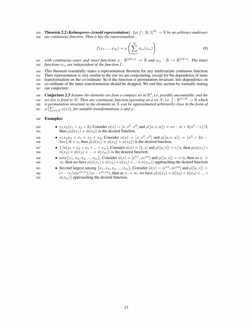
Theorem 2.2 (Kolmogorov–Arnold representation) Let f : [0, 1]M → R be an arbitrary multivari-539

ate continuous function. Then it has the representation540

f(x1, ..., xM ) = ρ

(M∑m=1

φm(xm)

)(8)

with continuous outer and inner functions ρ : R2M+1 → R and φm : R → R2M+1. The inner541

functions φm are independent of the function f .542

This theorem essentially states a representation theorem for any multivariate continous function.543

Their representation is very similar to the one we are conjecturing, except for the dependence of inner544

transformation on the co-ordinate. So if the function is permutation invariant, this dependence on545

co-ordinate of the inner transformation should be dropped. We end this section by formally stating546

our conjecture:547

Conjecture 2.3 Assume the elements are from a compact set in Rd, i.e. possibly uncountable, and the548

set size is fixed to M . Then any continuous function operating on a set X , i.e. f : Rd×M → R which549

is permutation invariant to the elements in X can be approximated arbitrarily close in the form of550

ρ(∑

x∈X φ(x)), for suitable transformations φ and ρ.551

Examples:552

• x1x2(x1 + x2 + 3), Consider φ(x) = [x, x2, x3] and ρ([u, v, w]) = uv−w+ 3(u2− v)/2,553

then ρ(φ(x1) + φ(x2)) is the desired function.554

• x1x2x3 + x1 + x2 + x3, Consider φ(x) = [x, x2, x3] and ρ([u, v, w]) = (u3 + 2w −555

3uv)/6 + u, then ρ(φ(x1) + φ(x2) + φ(x3)) is the desired function.556

• 1/n(x1 +x2 +x3 + ...+xm), Consider φ(x) = [1, x] and ρ([u, v]) = v/u, then ρ(φ(x1) +557

φ(x2) + φ(x3) + ...+ φ(xm)) is the desired function.558

• max{x1, x2, x3, ..., xm}, Consider φ(x) = [eαx, xeαx] and ρ([u, v]) = v/u, then as α →559

∞, then we have ρ(φ(x1)+φ(x2)+φ(x3)+ ...+φ(xm)) approaching the desired function.560

• Second largest among {x1, x2, x3, ..., xm}, Consider φ(x) = [eαx, xeαx] and ρ([u, v]) =561

(v− (v/u)eαv/u)/(u− eαv/u), then as α→∞, we have ρ(φ(x1) + φ(x2) + φ(x3) + ...+562

φ(xm)) approaching the desired function.563

13

B Proof of Lemma 3564

Our goal is to design neural network layers that are equivariant to permutations of elements in the565

input x. The function f : XM → YM is equivariant to the permutation of its inputs iff566

f(πx) = πf(x) ∀π ∈ SNwhere the symmetric group SN is the set of all permutation of indices 1, . . . , N .567

Consider the standard neural network layer568

fΘ(x).= σ(Θx) Θ ∈ RN×N (9)

where Θ is the weight vector and σ : R→ R is a nonlinearity such as sigmoid function. The following569

lemma states the necessary and sufficient conditions for permutation-equivariance in this type of570

function.571

Lemma 3 The function fΘ : RM → RM as defined in (9) is permutation equivariant if and only if572

all the off-diagonal elements of Θ are tied together and all the diagonal elements are equal as well.573

That is,574

Θ = λI + γ (11T) λ, γ ∈ R 1 = [1, . . . , 1]T ∈ RN

where I ∈ RN×N is the identity matrix.575

Proof.576

From definition of permutation equivariance fΘ(πx) = πfΘ(x) and definition of f in (9), the577

condition becomes σ(Θπx) = πσ(Θx), which (assuming sigmoid is a bijection) is equivalent to578

Θπ = πΘ. Therefore we need to show that the necessary and sufficient conditions for the matrix579

Θ ∈ RM×M to commute with all permutation matrices π ∈ SM is given by this proposition. We580

prove this in both directions:581

• To see why Θ = λI + γ (11T) commutes with any permutation matrix, first note thatcommutativity is linear – that is

Θ1π = πΘ1 ∧Θ2π = πΘ2 ⇒ (aΘ1 + bΘ2)π = π(aΘ1 + bΘ2).

Since both Identity matrix I, and constant matrix 11T, commute with any permutation582

matrix, so does their linear combination Θ = λI + γ (11T).583

• We need to show that in a matrix Θ that commutes with “all” permutation matrices584

– All diagonal elements are identical: Let πk,l for 1 ≤ k, l ≤M,k 6= l, be a transposition585

(i.e. a permutation that only swaps two elements). The inverse permutation matrix of586

πk,l is the permutation matrix of πl,k = πTk,l. We see that commutativity of Θ with the587

transposition πk,l implies that Θk,k = Θl,l:588

πk,lΘ = Θπk,l ⇒ πk,lΘπl,k = Θ ⇒ (πk,lΘπl,k)l,l = Θl,l ⇒ Θk,k = Θl,l

Therefore, π and Θ commute for any permutation π, they also commute for any589

transposition πk,l and therefore Θi,i = λ ∀i.590

– All off-diagonal elements are identical: We show that since Θ commutes with any591

product of transpositions, any choice two off-diagonal elements should be identical.592

Let (i, j) and (i′, j′) be the index of two off-diagonal elements (i.e. i 6= j and i′ 6= j′).593

Moreover for now assume i 6= i′ and j 6= j′. Application of the transposition πi,i′Θ,594

swaps the rows i, i′ in Θ. Similarly, Θπj,j′ switches the jth column with j′th column.595

From commutativity property of Θ and π ∈ Sn we have596

πj′,jπi,i′Θ = Θπj′,jπi,i′ ⇒ πj′,jπi,i′Θ(πj′,jπi,i′)−1 = Θ ⇒

πj′,jπi,i′Θπi′,iπj,j′ = Θ ⇒ (πj′,jπi,i′Θπi′,iπj,j′)i,j = Θi,j ⇒ Θi′,j′ = Θi,j

where in the last step we used our assumptions that i 6= i′, j 6= j′, i 6= j and i′ 6= j′. In597

the cases where either i = i′ or j = j′, we can use the above to show that Θi,j = Θi′′,j′′598

and Θi′,j′ = Θi′′,j′′ , for some i′′ 6= i, i′ and j′′ 6= j, j′, and conclude Θi,j = Θi′,j′ .599

600

601

14

C More Details on the architecture602

Invariant model. The structure of permutation invariant functions in Theorem 2 hints at a general603

strategy for inference over sets of objects, which we call deep sets. Replacing φ and ρ by universal604

approximators leaves matters unchanged, since, in particular, φ and ρ can be used to approximate arbi-605

trary polynomials. Then, it remains to learn these approximators. This yields in the following model:606

+

ϕρ

X

x1

x2

zOptional

conditioning

based on meta-

information

S(X)

Figure 4: Architecture of deep sets

607

• Each instance xm∀1 ≤ m ≤ M is608

transformed (possibly by several lay-609

ers) into some representation φ(xm).610

• The addition∑m φ(xm) of these rep-611

resentations processed using the ρ net-612

work very much in the same manner613

as in any deep network (e.g. fully con-614

nected layers, nonlinearities, etc).615

• Optionally: If we have additional meta-616

information z, then the above men-617

tioned networks could be conditioned618

to obtain the conditioning mapping619

φ(xm|z).620

In other words, the key to deep sets is to add up621

all representations and then apply nonlinear transformations.622

The overall model structure is illustrated in Fig. 4.623

This architecture has a number of desirable properties in terms of universality and correctness. We624

assume in the following that the networks we choose are, in principle, universal approximators. That625

is, we assume that they can represent any functional mapping. This is a well established property (see626

e.g. [48] for details in the case of radial basis function networks).627

What remains is to state the derivatives with regard to this novel type of layer. Assume parametrizations628

wρ and wφ for ρ and φ respectively. Then we have629

∂wφρ

(∑x′∈X

φ(x′)

)= ρ′

(∑x′∈X

φ(x)

) ∑x′∈X

∂wφφ(x′)

This result reinforces the common knowledge of parameter tying in deep networks when ordering is630

irrelevant. Our result backs this practice with theory and strengthens it by proving that it is the only631

way to do it.632

Equivariant model. Consider the standard neural network layer633

fΘ(x) = σ(Θx) (10)

where Θ ∈ RM×M is the weight vector and σ : RM → RM is a point-wise nonlinearity such as a634

sigmoid function. The following lemma states the necessary and sufficient conditions for permutation-635

equivariance in this type of function.636

Lemma 3 The function fΘ(x) = σ(Θx) for Θ ∈ RM×M is permutation equivariant, iff all the637

off-diagonal elements of Θ are tied together and all the diagonal elements are equal as well. That is,638

Θ = λI + γ (11T) λ, γ ∈ R 1 = [1, . . . , 1]T ∈ RM

where I ∈ RM×M is the identity matrix.639

This function is simply a non-linearity applied to a weighted combination of i) its input Ix and; ii)640

the sum of input values (11T)x. Since summation does not depend on the permutation, the layer is641

permutation-equivariant. Therefore we can manipulate the operations and parameters in this layer,642

for example to get another variation f(x) = σ (λIx + γ maxpool(x)1), where the maxpooling643

operation over elements of the set (similarly to summation) is commutative. In practice using this644

variation performs better in some applications.645

So far we assumed that each instance xm ∈ R – i.e. a single input and also output chan-646

nel. For multiple input-output channels, we may speed up the operation of the layer using647

15

matrix multiplication. For D/D′ input/output channels (i.e. x ∈ RM×D, y ∈ RM×D′ , this648

layer becomes f(x) = σ(xΛ − 1xmaxΓ

)where Λ,Γ ∈ RD×D′ are model parameters and649

xmax = (maxm x) ∈ R1×D is a row-vector of maximum value of x over the “set” dimension.650

We may further reduce the number of parameters in favor of better generalization by factoring Γ and651

Λ and keeping a single Λ ∈ RD,D′ and β ∈ RD′652

f(x) = σ(β +

(x − 1(max

mx))Γ)

(11)

Since composition of permutation equivariant functions is also permutation equivariant, we can build653

deep models by stacking layers of (11). Moreover, application of any commutative pooling operation654

(e.g. max-pooling) over the set instances produces a permutation invariant function.655

16

D Bayes Set656

Bayesian sets consider the problem of estimating the likelihood of subsets X of a ground set X . In657

general this is achieved by an exchangeable model motivated by deFinetti’s theorem concerning658

exchangeable distributions via659

p(X|α) =

∫dθ

[m∏i=1

p(xi|θ)

]p(θ|α). (12)

This allows one to perform set expansion, simply via the score660

s(x|X) = logp(X ∪ {x} |α)

p(X|α)p({x} |α)(13)

Note that s(x|X) is the pointwise mutual information between x and X . Moreover, due to exchange-661

ability, it follows that regardless of the order of elements we have662

S(X) :=

m∑i=1

s (xi| {xi−1, . . . x1}) = log p(X|α)−m∑i=1

log p({xi} |α) (14)

In other words, we have a set function log p(X|α) with a modular term-dependent correction. When663

inferring sets it is our goal to find set completions {xn+1, . . . xm} for an initial set of query terms664

{x1, . . . , xn} such that the aggregate set is well coherent. This is the key idea of the Bayesian Set665

algorithm.666

D.1 Exponential Family667

In exponential families, the above approach assumes a particularly nice form whenever we have668

conjugate priors. Here we have669

p(x|θ) = exp (〈φ(x), θ〉 − g(θ)) and p(θ|α,m0) = exp (〈θ, α〉 −m0g(θ)− h(α,m0)) . (15)The mapping φ : x→ F is usually referred as sufficient statistic of x which maps x into a feature670

space F . Moreover, g(θ) is the log-partition (or cumulant-generating) function. Finally, p(θ|α)671

denotes the onjugate distribution which is in itself a member of the exponential family. It has the672

normalization h(α) =∫dθ exp (〈θ, αµ〉 − αmg(θ)). The advantage of this is that s(x|X) and S(X)673

can be computed in closed form [49] via674

s(X) = h (α+ φ(X),m0 +m) + (m− 1)h(α,m0)−m∑i=1

h(α+ φ(xi),m+ 1) (16)

s(x|X) = h (α+ φ({x} ∪X),m0 +m+ 1) + h(α,m0) (17)− h (α+ φ(X),m0 +m)− h(α+ φ(x),m+ 1)

For convenience we defined the sufficient statistic of a set to be the sum over its constituents, i.e.675

φ(X) =∑i φ(xi). It allows for very simple computation and maximization over additional elements676

to be added to X , since φ(X) can be precomputed.677

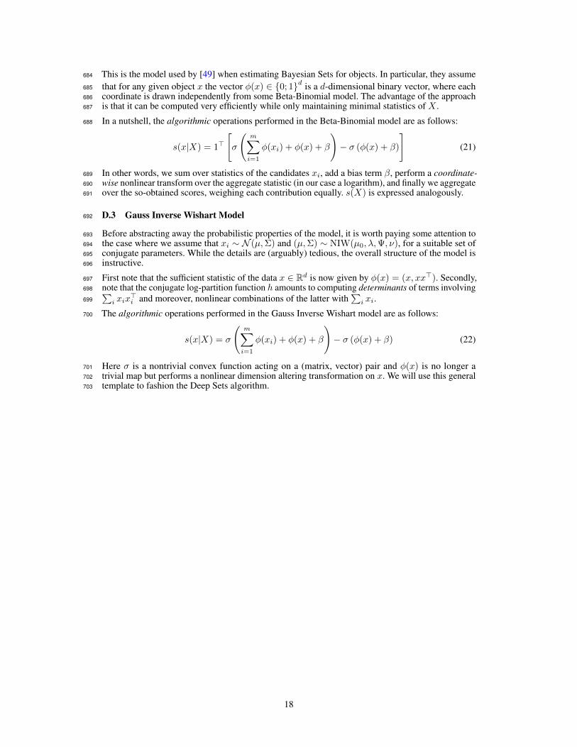
D.2 Beta-Binomial Model678

The model is particularly simple when dealing with the Binomial distribution and its conjugate Beta679

prior, since the ratio of Gamma functions allows for simple expressions. In particular, we have680

h(β) = log Γ(β+) + log Γ(β−)− Γ(β). (18)

With some slight abuse of notation we let α = (β+, β−) and m0 = β+ + β−. Setting φ(1) =681

(1, 0) and φ(0) = (0, 1) allows us to obtain φ(X) = (m+,m−), i.e. φ(X) contains the counts of682

occurrences of xi = 1 and xi = 0 respectively. This leads to the following score functions683

s(X) = log Γ(β+ +m+) + log Γ(β− +m−)− log Γ(β +m) (19)

− log Γ(β+)− log Γ(β−) + log Γ(β)− n+ logβ+

β− n− log

β−

β

s(x|X) =

{log β++m+

β+m − log β+

β if x = 1

log β−+m−

β+m − log β−

β otherwise(20)

17

This is the model used by [49] when estimating Bayesian Sets for objects. In particular, they assume684

that for any given object x the vector φ(x) ∈ {0; 1}d is a d-dimensional binary vector, where each685

coordinate is drawn independently from some Beta-Binomial model. The advantage of the approach686

is that it can be computed very efficiently while only maintaining minimal statistics of X .687

In a nutshell, the algorithmic operations performed in the Beta-Binomial model are as follows:688

s(x|X) = 1>

[σ

(m∑i=1

φ(xi) + φ(x) + β

)− σ (φ(x) + β)

](21)

In other words, we sum over statistics of the candidates xi, add a bias term β, perform a coordinate-689

wise nonlinear transform over the aggregate statistic (in our case a logarithm), and finally we aggregate690

over the so-obtained scores, weighing each contribution equally. s(X) is expressed analogously.691

D.3 Gauss Inverse Wishart Model692

Before abstracting away the probabilistic properties of the model, it is worth paying some attention to693

the case where we assume that xi ∼ N (µ,Σ) and (µ,Σ) ∼ NIW(µ0, λ,Ψ, ν), for a suitable set of694

conjugate parameters. While the details are (arguably) tedious, the overall structure of the model is695

instructive.696

First note that the sufficient statistic of the data x ∈ Rd is now given by φ(x) = (x, xx>). Secondly,697

note that the conjugate log-partition function h amounts to computing determinants of terms involving698 ∑i xix

>i and moreover, nonlinear combinations of the latter with

∑i xi.699

The algorithmic operations performed in the Gauss Inverse Wishart model are as follows:700

s(x|X) = σ

(m∑i=1

φ(xi) + φ(x) + β

)− σ (φ(x) + β) (22)

Here σ is a nontrivial convex function acting on a (matrix, vector) pair and φ(x) is no longer a701

trivial map but performs a nonlinear dimension altering transformation on x. We will use this general702

template to fashion the Deep Sets algorithm.703

18

E Text Concept Set Retrieval704

We consider the task of text concept set retrieval, where the objective is to retrieve words belonging705

to a ‘concept’ or ‘cluster’, given few words from that particular concept. For example, given the set706

of words {tiger, lion, cheetah}, we would need to retrieve other related words like jaguar, puma,707

etc, which belong to the same concept of big cats. The model implicitly needs to reason out the708

concept connecting the given set and then retrieve words based on their relevance to the inferred709

concept. Concept set retrieval is an important due to wide range of potential applications including710

personalized information retrieval, tagging large amounts of unlabeled or weakly labeled datasets,711

etc. This task of concept set retrieval can be seen as a set completion task conditioned on the latent712

semantic concept, and therefore our Deepsets form a desirable approach.713

Dataset To construct a large dataset containing sets of related words, we make use of Wikipedia714

text due to its huge vocabulary and concept coverage. First, we run topic modeling on publicly715

available wikipedia text with K number of topics. Specifically, we use the famous latent Dirichlet716

allocation [37, 38], taken out-of-the-box4. Next, we choose top NT = 50 words for each latent topic717

as a set giving a total of K sets of size NT . To compare across scales, we consider three values718

of k = {1k, 3k, 5k} giving us three datasets LDA-1k, LDA-3k, and LDA-5k, with corresponding719

vocabulary sizes of 17k, 38k, and 61k. Few of the topics from LDA-1k are visualized in Tab. 5.720

Methods Our Deepsets model uses a feedforward neural network (NN) to represent a query and721

each element of a set, i.e., φ(x) for an element x is encoded as a NN. We then construct a set722

representation or feature, by sum pooling all the individual representations of its elements, along with723

that of the query. Note that this sum pooling achieves permutation invariance, a crucial property of724

our Deepsets (Theorem 2). Next, use input this set feature into another NN to assign a single score725

to the set, shown as ρ(.). In summary, our Deepsets consists of two neural networks – (a) to extract726

representations for each element, and (b) to score a set after pooling representations of its elements.727

Baselines We compare to several baselines: (a) Random picks a word from the vocabulary uni-728

formly at random. (b) Bayes Set [35], and (c) w2v-Near that computes the nearest neighbors in729

the word2vec [39] space. Note that both Bayes Set and w2v NN are strong baselines. The former730

runs Bayesian inference using Beta-Binomial conjugate pair, while the latter uses the powerful 300731

dimensional word2vec trained on the billion word GoogleNews corpus5. (d) NN-max uses a similar732

architecture as our Deepsets with an important difference. It uses max pooling to compute the set733

feature, as opposed to Deepsets which uses sum pooling. (e) NN-max-con uses max pooling on set734

elements but concatenates this pooled representation with that of query for a final set feature. (f)735

NN-sum-con is similar to NN-max-con but uses sum pooling followed by concatenation with query736

representation.737

Evaluation To quantitatively evaluate, we consider the standard retrieval metrics – recall@K,738

median rank and mean reciprocal rank. To elaborate, recall@K measures the number of true labels739

that were recovered in the top K retrieved words. We use three values of K = {10, 100, 1k}. The740

other two metrics, as the names suggest, are the median and mean of reciprocals of the true label741

ranks, respectively. Each dataset is split into TRAIN (80%), VAL (10%) and TEST (10%). We learn742

models using TRAIN and evaluate on TEST, while VAL is used for hyperparameter selection and743

early stopping.744

Results and Observations Tab. 3 contains the results for the text concept set retrieval on LDA-745

1k, LDA-3k, and LDA-5k datasets. We summarize our findings below: (a) Our Deepsets model746

outperforms all other approaches on LDA-3k and LDA-5k by any metric, highlighting the significance747

of permutation invariance property. For instance, Deepsets is better than the w2v-Near baseline by748

1.5% in Recall@10 on LDA-5k. (b) On LDA-1k, neural network based models do not perform well749

when compared to w2v-Near. We hypothesize that this is due to small size of the dataset insufficient750

to train a high capacity neural network, while w2v-Near has been trained on a billion word corpus.751

Nevertheless, our approach comes the closest to w2v-Near amongst other approaches, and is only752

0.5% lower by Recall@10.753

4github.com/dmlc/experimental-lda5code.google.com/archive/p/word2vec/

19

Topic 1legend

airytale

witchdevilgiantstory

folklore

Topic 2president

viceservedoffice

electedsecretary

presidencypresidential

Topic 3plan

proposedplans

proposalplanningapprovedplanned

development

Topic 4newspaper

dailypapernewspress

publishednewspapers

editor

Topic 5roundteamsfinal

playedredirect

woncompetitiontournament

Topic 6pointangleaxis

planedirectiondistancesurfacecurve

Figure 5: Examples from our LDA-1k datasets. Notice that each of these are latent topics of LDA andhence are semantically similar.

F Image Tagging754

We next experiment with image tagging, where the task is to retrieve all relevant tags corresponding755

to an image. Images usually have only a subset of relevant tags, therefore predicting other tags can756

help enrich information that can further be leveraged in a downstream supervised task. In our setup,757

we learn to predict tags by conditioning Deepsets on the image. Specifically, we train by learning to758

predict a partial set of tags from the image and remaining tags. At test time, we the test image is used759

to predict relevant tags.760

Datasets We report results on the following three datasets:761

(a) ESPgame [50]: Contains around 20k images spanning logos, drawings, and personal photos,762

collected interactively as part of a game. There are a total of 268 unique tags, with each image having763

4.6 tags on average and a maximum of 15 tags.764

(b) IAPRTC-12.5 [51]: Comprises of around 20k images including pictures of different sports and765

actions, photographs of people, animals, cities, landscapes, and many other aspects of contemporary766

life. A total of 291 unique tags have been extracted from captions for the images. For the above two767

datasets, train/test splits are similar to those used in previous works [43, 40].768

(c) COCO-Tag: We also construct a dataset in-house, based on MSCOCO dataset[52]. COCO is769

a large image dataset containing around 80k train and 40k test images, along with five caption770

annotations. We extract tags by first running a standard spell checker6 and lemmatizing these captions.771

Stopwords and numbers are removed from the set of extracted tags. Each image has 15.9 tags on an772

average and a maximum of 46 tags. We show examples of image tags from COCO-Tag in Fig. 6. The773

advantages of using COCO-Tag are three fold–richer concepts, larger vocabulary and more tags per774

image, making this an ideal dataset to learn image tagging using Deepsets.775

Image and Word Embeddings Our models use features extracted from Resnet, which is the776

state-of-the-art convolutional neural network (CNN) on ImageNet 1000 categories dataset using the777

publicly available 152-layer pretrained model7. To represent words, we jointly learn embeddings with778

the rest of Deepsets neural network for ESPgame and IAPRTC-12.5 datasets. But for COCO-Tag,779

we bootstrap from 300 dimensional word2vec embeddings8 as the vocabulary for COCO-Tag is780

significantly larger than both ESPgame and IAPRTC-12.5 (13k vs 0.3k).781

Methods The setup for Deepsets to tag images is similar to that described in Appendix E. The only782

difference being the conditioning on the image features, which is concatenated with the set feature783

obtained from pooling individual element representations. The resulting feature forms the new input784

to a neural network used to score the set, in this case, score the relevance of a tag to the image.785

Baselines We perform comparisons against several baselines, previously reported from [40]. Specif-786

ically, we have Least Sq., a ridge regression model, MBRM [41], JEC [42] and FastTag [40]. Note787

that these methods do not use deep features for images, which could lead to an unfair comparison. As788

there is no publicly available code for MBRM and JEC, we cannot get performances of these models789

with Resnet extracted features. However, we report results with deep features for FastTag and Least790

Sq., using code made available by the authors 9.791

Evaluation For ESPgame and IAPRTC-12.5, we follow the evaluation metrics as in [43] – precision792

(P), recall (R), F1 score (F1) and number of tags with non-zero recall (N+). Note that these metrics793

are evaluate for each tag and the mean is reported. We refer to [43] for further details. For COCO-Tag,794

6http://hunspell.github.io/7github.com/facebook/fb.resnet.torch8https://code.google.com/p/word2vec/9http://www.cse.wustl.edu/~mchen/

20

however, we use recall@K for three values of K = {10, 100, 1000}, along with median rank and795

mean reciprocal rank (see evaluation in Appendix E for metric details).796

Results and Observations Tab. 4 contains the results of image tagging on ESPgame and IAPRTC-797

12.5, and Tab. 5 on COCO-Tag. Here are the key observations from Tab. 4: (a) The performance798

of Deepsets is comparable to the best of other approaches on all metrics but precision. (b) Our799

recall beats the best approach by 2% in ESPgame. On further investigation, we found that Deepsets800

retrieves more relevant tags, which are not present in list of ground truth tags due to a limited 5 tag801

annotation. Thus, this takes a toll on precision while gaining on recall, yet yielding improvement in802

F1. On the larger and richer COCO-Tag, we see that Deepsets approach outperforms other methods803

comprehensively, as expected. We show qualitative examples in Fig. 6.804

GT Predbuilding building

sign streetbrick city

picture brickempty sidewalkwhite sideblack polestreet whiteimage stone

GT Predstanding personsurround groupwoman mancrowd tablewine sit

person roomgroup womantable couplebottle gather

GT Predtraffic clockcity tower

building skytall building

large talltower large

European cloudyfront frontclock city

GT Predphotograph ski

snowboarder snowsnow slopeglide personhill snowy

show hillperson manslope skiingyoung skier

GT Predlaptop refrigeratorperson fridgescreen roomroom magnetdesk cabinetliving kitchen

counter shelfcomputer wallmonitor counter

GT Predbeach jet

shoreline airplanestand propellerwalk oceansand plane

lifeguard waterwhite bodyperson person

surfboard sky

Figure 6: Qualitative examples of image tagging using Deepsets. Top row: Positive examples wheremost of the retrieved tags are present in the ground truth (brown) or are relevant but not present in theground truth (green). Bottom row: Few failure cases with irrelevant/wrong tags (red). From left toright, (i) Confusion between snowboarding and skiing, (ii) Confusion between back of laptop andrefrigerator due to which other tags are kitchen-related, (iii) Hallucination of airplane due to similarshape of surfboard.

We present examples of our in-house tagging datasets, COCO-Tag in Fig. 6.805

21

G Improved Red-shift Estimation Using Clustering Information806

An important regression problem in cosmology is to estimate the red-shift of galaxies, corresponding807

to their age as well as their distance from us [32]. Two common types of observation for distant808

galaxies include a) photometric and b) spectroscopic observations, where the latter can produce more809

accurate red-shift estimates.810

One way to estimate the red-shift from photometric observations is using a regression model [33].811

We use a multi-layer Perceptron for this purpose and use the more accurate spectroscopic red-shift812

estimates as the ground-truth. As another baseline, we have a photometric redshift estimate that813

is provided by the catalogue and uses various observations (including clustering information) to814

estimate individual galaxy-red-shift. Our objective is to use clustering information of the galaxies to815

improve our red-shift prediction using the multi-layer Preceptron.816

Note that the prediction for each galaxy does not change by permuting the members of the galaxy817

cluster. Therefore, we can treat each galaxy cluster as a “set” and use permutation-equivariant layer818

to estimate the individual galaxy red-shifts.819

For each galaxy, we have 17 photometric features 10 from the redMaPPer galaxy cluster catalog [34],820

which contains photometric readings for 26,111 red galaxy clusters. In this task in contrast to the821

previous ones, sets have different cardinalities; each galaxy-cluster in this catalog has between822

∼ 20−300 galaxies – i.e. x ∈ RN(c)×17, whereN(c) is the cluster-size. See Fig. 7(a) for distribution823

of cluster sizes. The catalog also provides accurate spectroscopic red-shift estimates for a subset of824

these galaxies as well as photometric estimates that uses clustering information. Fig. 7(b) reports the825

distribution of available spectroscopic red-shift estimates per cluster.826

We randomly split the data into 90% training and 10% test clusters, and use the following simple827

architecture for semi-supervised learning. We use four permutation-equivariant layers with 128, 128,828

128 and 1 output channels respectively, where the output of the last layer is used as red-shift estimate.829

The squared loss of the prediction for available spectroscopic red-shifts is minimized.11 Fig. 7(c)830

shows the agreement of our estimates with spectroscopic readings on the galaxies in the test-set with831

spectroscopic readings. The figure also compares the photometric estimates provided by the catalogue832

[34], to the ground-truth. As it is customary in cosmology literature, we report the average scatter833|zspec−z|1+zspec

, where zspec is the accurate spectroscopic measurement and z is a photometric estimate. The834

average scatter using our model is .023 compared to the scatter of .025 in the original photometric835

estimates for the redMaPPer catalog. Both of these values are averaged over all the galaxies with836

spectroscopic measurements in the test-set.837

We repeat this experiment, replacing the permutation-equivariant layers with fully connected layers838

(with the same number of parameters) and only use the individual galaxies with available spectroscopic839

estimate for training. The resulting average scatter for multi-layer Perceptron is .026, demonstrating840

that using clustering information indeed improves photometric red-shift estimates.841

Figure 7: application of permutation-equivariant layer to semi-supervised red-shift prediction using clusteringinformation: a) distribution of cluster (set) size; b) distribution of reliable red-shift estimates per cluster; c)prediction of red-shift on test-set (versus ground-truth) using clustering information as well as RedMaPPerphotometric estimates (also using clustering information).

10We have a single measurement for each u,g,r, i and z band as well as measurement error bars, location ofthe galaxy in the sky, as well as the probability of each galaxy being the cluster center. We do not include theinformation regarding the richness estimates of the clusters from the catalog, for any of the methods, so thatbaseline multi-layer Preceptron is blind to the clusters.

11We use mini-batches of size 128, Adam [53], with learning rate of .001, β1 = .9 and β2 = .999. All layersexcept for the last layer use Tanh units and simultaneous dropout with 50% dropout rate.

22

Figure 8: Examples for 8 out of 40 object classes (column) in the ModelNet40. Each point-cloud is produces bysampling 1000 particles from the mesh representation of the original MeodelNet40 instances. Two point-cloudsin the same column are from the same class. The projection of particles into xy, zy and xz planes are added forbetter visualization.

H Point Cloud Classification842

Tab. 6 presents a more detailed result on classification performance, using different techniques. Fig. 8843

shows examples of the dataset used for training. Fig. 9 shows the features learned by the first and844

second layer of our deep model. Here, we review the details of architectures used in the experiments.845

Deep-Set. We use a network comprising of 3 permutation-equivariant layers with 256 channels846

followed by max-pooling over the set structure. The resulting vector representation of the set is847

then fed to a fully connected layer with 256 units followed by a 40-way softmax unit. We use Tanh848

activation at all layers and dropout on the layers after set-max-pooling (i.e. two dropout operations)849

with 50% dropout rate. Applying dropout to permutation-equivariant layers for point-cloud data850

deteriorated the performance. We observed that using different types of permutation-equivariant851

layers (see Appendix C) and as few as 64 channels for set layers changes the result by less than 5%852

in classification accuracy.853

For the setting with 5000 particles, we increase the number of units to 512 in all layers and randomly854

rotate the input around the z-axis. We also randomly scale the point-cloud by s ∼ U(.8, 1./.8). For855

this setting only, we use Adamax [53] instead of Adam and reduce learning rate from .001 to .0005.856

Graph convolution. For each point-cloud instance with 1000 particles, we build a sparse K-nearest857

neighbor graph and use the three point coordinates as input features. We normalized all graphs858

at the preprocessing step. For direct comparison with set layer, we use the exact architecture of 3859

graph-convolution layer followed by set-pooling (global graph pooling) and dense layer with 256860

units. We use exponential linear activation function instead of Tanh as it performs better for graphs.861

Due to over-fitting, we use a heavy dropout of 50% after graph-convolution and dense layers. Similar862

to dropout for sets, all the randomly selected features are simultaneously dropped across the graph863

nodes. the We use a mini-batch size of 64 and Adam for optimization where the learning rate is .001864

(the same as that of permutation-equivariant counter-part).865

Despite our efficient sparse implementation using Tensorflow, graph-convolution is significantly866

slower than the set layer. This prevented a thorough search for hyper-parameters and it is quite867

possible that better hyper-parameter tuning would improve the results that we report here.868

Table 6: Classification accuracy and the (size of) representation used by different methods on the ModelNet40dataset.

model instance size representation accuracyDeep-Sets + transformation (ours) 5000× 3 point-cloud 90± .3%

Deep-Sets (ours) 1000× 3 point-cloud 87± 1%

Deep-Sets w. pooling only (ours) 1000× 3 point-cloud 83± 1%

Deep-Sets (ours) 100× 3 point-cloud 82± 2%

KNN graph-convolution (ours) 1000× (3 + 8) directed 8-regular graph 58± 2%

3DShapeNets [24] 303 voxels (using convolutional deep belief net) 77%

DeepPano [20] 64× 160 panoramic image (2D CNN + angle-pooling) 77.64%

VoxNet [25] 323 voxels (voxels from point-cloud + 3D CNN) 83.10%

MVCNN [21] 164× 164× 12 multi-vew images (2D CNN + view-pooling) 90.1%

VRN Ensemble [26] 323 voxels (3D CNN, variational autoencoder) 95.54%

3D GAN [27] 643 voxels (3D CNN, generative adversarial training) 83.3%

23

Tab. 6 compares our method against the competition.12 Note that we achieve our best accuracy using869

5000× 3 dimensional representation of each object, which is much smaller than most other methods.870

All other techniques use either voxelization or multiple view of the 3D object for classification.871

Interestingly, variations of view/angle-pooling, as in [21, 20], can be interpreted as set-pooling872

where the class-label is invariant to permutation of different views. The results also shows that873

using fully-connected layers with set-pooling alone (without max-normalization over the set) works874

relatively well.875

We see that reducing the number of particles to only 100, still produces comparatively good results.876

Using graph-convolution is computationally more challenging and produces inferior results in this877

setting. The results using 5000 particles is also invariant to small changes in scale and rotation around878

the z-axis.879

Figure 9: Each box is the particle-cloud maximizing the activation of a unit at the firs (top) and second (bottom)permutation-equivariant layers of our model. Two images of the same column are two different views of the samepoint-cloud.

Features. To visualize the features learned by the set layers, we used Adamax [53] to locate 1000880

particle coordinates maximizing the activation of each unit.13 Activating the tanh units beyond the881

second layer proved to be difficult. 9 shows the particle-cloud-features learned at the first and second882

layers of our deep network. We observed that the first layer learns simple localized (often cubic)883

point-clouds at different (x, y, z) locations, while the second layer learns more complex surfaces884

with different scales and orientations.885

I Set Anomaly Detection886

Our model has 9 convolution layers with 3× 3 receptive fields. The model has convolution layers887

with 32, 32, 64 feature-maps followed by max-pooling followed by 2D convolution layers with888

64, 64, 128 feature-maps followed by another max-pooling layer. The final set of convolution layers889

have 128, 128, 256 feature-maps, followed by a max-pooling layer with pool-size of 5 that reduces890

the output dimension to batch− size.N × 256, where the set-size N = 16. This is then forwarded891

to three permutation-equivariant layers with 256, 128 and 1 output channels. The output of final892

layer is fed to the Softmax, to identify the outlier. We use exponential linear units [54], drop out893

with 20% dropout rate at convolutional layers and 50% dropout rate at the first two set layers. When894

applied to set layers, the selected feature (channel) is simultaneously dropped in all the set members895

of that particular set. We use Adam [53] for optimization and use batch-normalization only in the896

convolutional layers. We use mini-batches of 8 sets, for a total of 128 images per batch.897

12The error-bar on our results is due to variations depending on the choice of particles during test time and itis estimated over three trials.

13We started from uniformly distributed set of particles and used a learning rate of .01 for Adamax, with firstand second order moment of .1 and .9 respectively. We optimized the input in 105 iterations. The results ofFig. 9 are limited to instances where tanh units were successfully activated. Since the input at the first layer ofour deep network is normalized to have a zero mean and unit standard deviation, we do not need to constrain theinput while maximizing unit’s activation.

24

Figure 10: Each row shows a set, constructed from CelebA dataset, such that all set members except for anoutlier, share at least two attributes (on the right). The outlier is identified with a red frame. The model istrained by observing examples of sets and their anomalous members, without access to the attributes. Theprobability assigned to each member by the outlier detection network is visualized using a red bar at the bottomof each image.

25

Figure 11: Each row of the images shows a set, constructed from CelebA dataset images, such that all setmembers except for an outlier, share at least two attributes. The outlier is identified with a red frame. The modelis trained by observing examples of sets and their anomalous members and without access to the attributes. Theprobability assigned to each member by the outlier detection network is visualized using a red bar at the bottomof each image. The probabilities in each row sum to one.

26