262
Subject Area: Management and Customer Relations Defining a Resilient Business Model for Water Utilities

Subject Area: Management and Customer Relations
Defining a Resilient Business Model for Water Utilities

Defining a Resilient Business Model for Water Utilities
©2014 Water Research Foundation. ALL RIGHTS RESERVED.

About the Water Research Foundation The Water Research Foundation (WRF) is a member-supported, international, 501(c)3 nonprofit organization that sponsors research that enables water utilities, public health agencies, and other professionals to provide safe and affordable drinking water to consumers. WRF’s mission is to advance the science of water to improve the quality of life. To achieve this mission, WRF sponsors studies on all aspects of drinking water, including resources, treatment, and distribution. Nearly 1,000 water utilities, consulting firms, and manufacturers in North America and abroad contribute subscription payments to support WRF’s work. Additional funding comes from collaborative partnerships with other national and international organizations and the U.S. federal government, allowing for resources to be leveraged, expertise to be shared, and broad-based knowledge to be developed and disseminated. From its headquarters in Denver, Colorado, WRF’s staff directs and supports the efforts of more than 800 volunteers who serve on the board of trustees and various committees. These volunteers represent many facets of the water industry, and contribute their expertise to select and monitor research studies that benefit the entire drinking water community. Research results are disseminated through a number of channels, including reports, the Website, Webcasts, workshops, and periodicals. WRF serves as a cooperative program providing subscribers the opportunity to pool their resources and build upon each other’s expertise. By applying WRF research findings, subscribers can save substantial costs and stay on the leading edge of drinking water science and technology. Since its inception, WRF has supplied the water community with more than $460 million in applied research value. More information about WRF and how to become a subscriber is available at www.WaterRF.org.
©2014 Water Research Foundation. ALL RIGHTS RESERVED.

Defining a Resilient Business Model for Water Utilities
Prepared by: Jeff Hughes, Mary Tiger, Shadi Eskaf, Stacey Isaac Berahzer, Sarah Royster, Christine Boyle, and Dayne Batten Environmental Finance Center at the University of North Carolina at Chapel Hill, Chapel Hill, NC 27599-3330 Peiffer Brandt and Catherine Noyes
Raftelis Financial Consultants, Inc., 1031 South Caldwell St., Suite 100, Charlotte, NC 28203 Jointly sponsored by: Water Research Foundation 6666 West Quincy Avenue, Denver, CO 80235 and U.S. Environmental Protection Agency Washington D.C. Published by:
DISCLAIMER This study was jointly funded by the Water Research Foundation (WRF) and U.S.
Environmental Protection Agency (EPA) under Cooperative Agreement No. EM-83484801-0. WRF and EPA assume no responsibility for the content of the research study reported in this publication or for the opinions or statements of fact expressed in the report. The mention of
trade names for commercial products does not represent or imply the approval or endorsement of the Foundation or EPA. This report is presented solely for informational
purposes.
Copyright ©2014
by Water Research Foundation
ALL RIGHTS RESERVED. No part of this publication may be copied, reproduced
or otherwise utilized without permission.
ISBN 978-1-60573-199-5
Printed in the U.S.A.
©2014 Water Research Foundation. ALL RIGHTS RESERVED.

v
CONTENTS
LIST OF TABLES ......................................................................................................................... ix
LIST OF FIGURES ....................................................................................................................... xi
FOREWORD ............................................................................................................................... xix
ACKNOWLEDGMENTS ........................................................................................................... xxi
EXECUTIVE SUMMARY ....................................................................................................... xxiii
CHAPTER 1: BACKGROUND AND METHODOLOGY ........................................................... 1Introduction ................................................................................................................... 1Focus ............................................................................................................................. 2Methodology ................................................................................................................. 3 Data collection, cleaning, and preparation .................................................................. 13References ................................................................................................................... 16
CHAPTER 2: ASSESSING THE REVENUE RESILIENCE OF THE INDUSTRY’S BUSINESS MODEL .................................................................................................................... 19
Trends In Financial Performance ...................................................................................... 19Introduction ................................................................................................................. 19Key Points ................................................................................................................... 20The Business Model Behind Utility Revenues ........................................................... 20National Trends in Total Operating Revenues ............................................................ 24 Statewide Trends in Total Operating Revenues .......................................................... 26 Examples of Utilities’ Trends in Total Operating Revenues ...................................... 28Trends in Utility Expenses .......................................................................................... 29Key Points ................................................................................................................... 30Utility Expenses Deconstructed .................................................................................. 30National Trends in Operating Expenses, Relative to Operating Revenues ................ 33Statewide Trends in Operating Expenses, Relative to Operating Revenues .............. 37Trends in Debt and Debt Service Coverage ................................................................ 41References ................................................................................................................... 43
Pricing Trends and Financial Resilience ........................................................................... 43Introduction ................................................................................................................. 43Key Points ................................................................................................................... 44Frequency of Rate Changes ........................................................................................ 45Degree of Rate Changes .............................................................................................. 50Cumulative Rate Changes ........................................................................................... 56Rate Increases at Different Consumption Levels ........................................................ 60Changes to Base Charges and Volumetric Rates ........................................................ 62Relationship between Rate Structures, Rate Increases, and Revenues ....................... 68Relationship of Rate Increases and Utility Financial Performance ............................ 72Conclusions ................................................................................................................. 75
©2014 Water Research Foundation. ALL RIGHTS RESERVED.

vi
References ................................................................................................................... 76
CHAPTER 3: FACTORS INFLUENCING REVENUE RESILIENCY ..................................... 77Service Area Size and Diversity ....................................................................................... 77
Introduction ................................................................................................................. 77Key Points ................................................................................................................... 77System Size ................................................................................................................. 77Diversity of Customer Base ........................................................................................ 80References ................................................................................................................... 82
Water Use And Weather ................................................................................................... 82Introduction ................................................................................................................. 82Key Points ................................................................................................................... 83National Trends ........................................................................................................... 83Regional Trends .......................................................................................................... 85The Impact of Weather and Droughts ......................................................................... 89Water Use, Rates, and Revenue .................................................................................. 91 Conclusion .................................................................................................................. 92
References ................................................................................................................... 92Economic Conditions ........................................................................................................ 93
Introduction ................................................................................................................. 93Key Points ................................................................................................................... 93Trends in Economic Conditions.................................................................................. 94References ................................................................................................................. 102
Capacity Utilization ........................................................................................................ 102Introduction ............................................................................................................... 102Key Points ................................................................................................................. 102Assessing Capacity Utilization ................................................................................. 103Capacity Utilization Trends ...................................................................................... 103Relationship Between Treatment Plant Capacity Utilization and Utility Financial
Condition............................................................................................................. 105Implications............................................................................................................... 108
Economic Regulation and Governance ........................................................................... 109Introduction ............................................................................................................... 109Key Points ................................................................................................................. 110Municipal/County-Owned Utilities .......................................................................... 111Independent Authorities and Districts ...................................................................... 111Private Investor-Owned Companies ......................................................................... 111Government-Owned Utilities Regulated by a Utility Commission .......................... 112Other Types of Economic Regulation and Oversight ............................................... 115Direct Impact on Financial Condition....................................................................... 116References ................................................................................................................. 119
Financial Management Strategies ................................................................................... 119Introduction ............................................................................................................... 119Key Points ................................................................................................................. 120Focus on Effective Utility Management as a Financial Management Driver ........... 120 Focus on LEAN as a Financial Management Driver ................................................ 121Utility Case Study ..................................................................................................... 121
©2014 Water Research Foundation. ALL RIGHTS RESERVED.

vii
References ................................................................................................................. 122Credit Rating Agencies ................................................................................................... 122
Introduction ............................................................................................................... 122Key Points ................................................................................................................. 123Reflection of Financial Position of Individual Water Utilities and the Industry as a
Whole .................................................................................................................. 123Other Players ............................................................................................................. 124No Formulas, Just Considerations ............................................................................ 125Financial Focus on Flexibility, Capacity, and Predictability .................................... 128Water Demand .......................................................................................................... 131Pricing and Rate Structures ....................................................................................... 132The Cart Leading the Horse: The Driving Power of Credit Rating Financial Metrics ................................................................................................................ 133Conclusion and Gap Analysis ................................................................................... 135References ................................................................................................................. 136
CHAPTER 4: STRATEGIES AND PRACTICES FOR REVENUE RESILIENCY ................ 139Demand Projections ........................................................................................................ 139
Introduction ............................................................................................................... 139Key Points ................................................................................................................. 140Practices for Improving Revenue Projections Linked to Sales ................................. 140Conclusion ................................................................................................................ 144References ................................................................................................................. 144
Alternative Rate Designs ................................................................................................ 145Introduction: Challenges of Current Rate Structures ................................................ 145Key Points ................................................................................................................. 146Justifying an Alternative ........................................................................................... 147 Modeling Alternatives .............................................................................................. 147Methodology ............................................................................................................. 149PeakSet Base Model ................................................................................................. 149CustomerSelect Model .............................................................................................. 152WaterWise Dividend Model ..................................................................................... 154Conclusion: Implementing Alternatives ................................................................... 155References ................................................................................................................. 155
Rate Stabilization Reserves............................................................................................. 157Introduction ............................................................................................................... 157Key Points ................................................................................................................. 157Purpose ...................................................................................................................... 158Types ......................................................................................................................... 158Targets and Governance ........................................................................................... 159Trends in Reserves .................................................................................................... 163Conclusions ............................................................................................................... 165References ................................................................................................................. 167
Rethinking Utility Services ............................................................................................. 169Introduction ............................................................................................................... 169Key Points ................................................................................................................. 169Focus on Service Line Protection Programs ............................................................. 170
©2014 Water Research Foundation. ALL RIGHTS RESERVED.
viii
Third-Party Approach to Service Line Protection Programs .................................... 170In-House Approach to Service Line Protection Programs ........................................ 172Focus on Public Fire Protection Charges .................................................................. 172Conclusions ............................................................................................................... 176References ................................................................................................................. 177
Financial Performance Targets ....................................................................................... 177Introduction ............................................................................................................... 177Key Points ................................................................................................................. 179Origin ........................................................................................................................ 179Uses ........................................................................................................................... 180Financial Impact of Financial Metrics ...................................................................... 183Conclusion ................................................................................................................ 184References ................................................................................................................. 185
Customer Affordability/Assistance Programs ................................................................ 186Introduction ............................................................................................................... 186Key Points ................................................................................................................. 186Defining Affordability .............................................................................................. 186Increasing Pressure to Manage Water with Affordability in Mind ........................... 187Types of Affordability Programs .............................................................................. 188State Laws Influence the Design of Affordability Programs .................................... 190How Much Will a Utility Spend on a Customer Affordability Program .................. 192Impact of Customer Affordability on Utility Operations ......................................... 195Customer Assistance in the Energy Sector ............................................................... 195Conclusions ............................................................................................................... 199References ................................................................................................................. 199
Rate Adjustment Approaches ......................................................................................... 201Introduction ............................................................................................................... 201Key Points ................................................................................................................. 202Cost-Indexed Rate Adjustments ............................................................................... 202Multi-year Rate Increases ......................................................................................... 208Pass-Through Charges .............................................................................................. 210Conclusion ................................................................................................................ 214References ................................................................................................................. 214
CHAPTER 5: CONCLUSIONS AND RECOMMENDATIONS .............................................. 217
ABBREVIATIONS .................................................................................................................... 219
ADDENDUMS ........................................................................................................................... 223A Financial Policy Strawman ................................................................................... 223 Credit Rating ........................................................................................................ 224 Debt ...................................................................................................................... 224 Operations ............................................................................................................ 225 Reserves ............................................................................................................... 226 Rates ..................................................................................................................... 226 References ............................................................................................................ 227B Catalog of Blog Posts ............................................................................................ 228
©2014 Water Research Foundation. ALL RIGHTS RESERVED.

ix
LIST OF TABLES
ES.1 Average trends in median increases to operating revenues in cohorts of utilities in six states ................................................................................................................................ xxv
ES.2 Utility Reserve Fund Targets ...........................................................................................xxx 1.1 Summary of national and state-level data sets on utility finances and rates used in this
research ....................................................................................................................7 2.1 Proportion of customer sales (base charges + commodity charges) collected from
commodity charges ................................................................................................24 2.2 Average trends in median increases to operating revenues in cohorts of utilities in six
states .......................................................................................................................28 2.3 Trends in total operating revenues in 18 utilities, FY2002-FY2011 .................................29 3.1 Utility financial performance in FY2012 among 382 local government utilities in North
Carolina, by utility size ..........................................................................................78 3.2 Median water and wastewater monthly bills in North Carolina in 2013, by utility size ...79 3.3 Tap fee revenues for seven Colorado utilities, FY2004 – FY2010 .................................102 3.4 Summary of Credit Rating Agency Guidance .................................................................124 3.5 Fitch Rating’s Key Financial Ratios ................................................................................126 3.6 Drought-time credit considerations by Fitch Ratings and assessment of utility control .132 3.7 Cost savings from interest rate differences due to credit rating .......................................134 4.1 Financial repercussions of demand projections ...............................................................140 4.2 Example PeakSet Base Model for the residential customers of BJWSA ........................150 4.3 Modeled water and irrigation schedule for CustomerSelect Model ................................153 4.4 Utility reserve fund targets ...............................................................................................160 4.5 Reserve fund size considerations .....................................................................................161
©2014 Water Research Foundation. ALL RIGHTS RESERVED.
x
4.6 Sample for calculating adjustments for water rates and services: Public fire protection............................................................................................173 4.7 Summary of financial metrics in water utility debt and financial policies ......................181 4.8 Coverage metrics included in Birmingham’s rate stabilization and equalization approach ...............................................................................................................184 4.9 What is the total annual cost to your utility for all assistance programs? ........................192 4.10 Customer affordability program details in three hypothetical water systems ..................193 4.11 Historical participation in Baltimore’s low income senior citizens discount ..................198 4.12 Historical participation in Baltimore’s low income assistance Crisis Intervention Grant
Program ................................................................................................................198
©2014 Water Research Foundation. ALL RIGHTS RESERVED.

xi
LIST OF FIGURES
ES.1 Map of utilities included in all utility financial and rates data sets ............................... xxiv ES.2 Annual changes to total operating revenues among the same 485 utilities nationwide ...xxv ES.3 Cumulative bill increases for 1,961 utilities in six states compared to regional CPI .... xxvi ES.4 Increases in rates and operating revenues for 94 utilities nationwide, 2004 to 2012 .. xxviii ES.5 Key credit rating considerations of S&P for 18 drinking water utilities from 2010-2012 ................................................................................................................... xxxix ES.6 Comparison of monthly and annual charges for a customer under a utility’s current rate
structure to an alternative rate (PeakSet Base) modeled rates for the same amount of water use ..........................................................................................................xxx
1.1 This report will focus on financial condition, revenues, and rates (model adapted from
Hendrick 2011) ........................................................................................................3 1.2 Four levels of data analysis in this report ............................................................................4 1.3 Map of utilities included in all utility financial and rates data sets ...................................13 2.1 Total operating revenues as a percent of total revenues among 662 utilities nationwide in
2012........................................................................................................................21 2.2 Revenues from customer sales as percent of total operating revenues in FY2011 ...........22 2.3 Layers of revenues and the proportion of revenues from commodity charges in two
utilities....................................................................................................................23 2.4 Annual change in total operating revenues among the same 485 utilities nationwide .....25 2.5 Annual changes to revenues among 2,838 utilities in six states. .......................................27 2.6 Total operating expenses as a percent of total expenses among 260 utilities nationwide .31 2.7 Fixed versus variable costs and revenues for two utilities .................................................32 2.8 Debt service as a percentage of total operating revenues for 126 water and combined
utilities from 2003-2012 ........................................................................................33 2.9 Total operating revenues and operation and maintenance expenses reported in 2012
compared to prior years among 517 utilities nationwide. ......................................34
©2014 Water Research Foundation. ALL RIGHTS RESERVED.

xii
2.10 Comparing annual changes to operating revenues and operation and maintenance expenses in the same 383 utilities nationwide .......................................................35
2.11 Non-capital operating ratios for the same 383 utilities nationwide ..................................36 2.12 Operating ratios for 529 utilities nationwide ....................................................................37 2.13 Trends in operating ratios among a cohort of 1,596 utilities in CA, GA and NC .............38 2.14 Trends in non-capital operating ratios among a cohort of 1,236 utilities in OH, TX and WI ....................................................................................................................38 2.15 Percent of utilities with operating expenses exceeding operating revenues. .....................40 2.16 Percent of utilities with operation and maintenance expenses exceeding operating
revenues .................................................................................................................40 2.17 Long-term debt for 192 water and combined utilities from 2003-2012 ............................41 2.18 Debt service coverage ratio for 126 water and combined utilities from 2003 – 2012 .......42 2.19 Debt service coverage ratio for 673 water and combined utilities by most recent credit
rating ......................................................................................................................43 2.20 Utilities changing water rates, 2000 – 2012 (n=318 utilities nationwide) .........................46 2.21 Frequency of water rate changes between biennial rates survey years between 2004 and
2012 for 58 utilities nationwide .............................................................................47 2.22 Percent of utilities changing rates in five states (n=3,102 utilities) ...................................48 2.23 Frequency of rate adjustments in 5 consecutive years among 1,966 utilities in five states49 2.24 Frequency of rate increases from 2006-2010 among 7 states ............................................50 2.25 Biennial nationwide rate modifications, 2000-2012 (n=329 utilities) ...............................51 2.26 Annualized increase to total monthly bill for 10 ccf for 72 utilities nationwide ...............52 2.27 Annual rate modifications of utilities that adjusted rates in five states .............................54 2.28 Average rate adjustment by frequency of raising rates among 1,966 utilities in five states55 2.29 Average 5-year cumulative rate increase by frequency of rate adjustments .....................56 2.30 Cumulative bill increases for 1,961 utilities in six states compared to CPI by region ......58
©2014 Water Research Foundation. ALL RIGHTS RESERVED.

xiii
2.31 Monthly charge for 10 ccf relative to 2004 charge for 72 nationwide utilities .................59 2.32 Credit rating vs. percent rate increase from 2006 to 2010 for 82 utilities nationwide ......60 2.33 Median monthly water bill by level of consumption for 58 nationwide utilities from
2004-2005 ..............................................................................................................61 2.34 Median monthly water bill by level of consumption for 1,292water utilities in North
Carolina, Georgia, and Wisconsin .........................................................................62 2.35 Statewide median of base charges as percent of total bills by consumption level in four
states .......................................................................................................................64 2.36 Charlotte-Mecklenburg Utilities’ shift towards greater fixed charges in residential bills in
2012........................................................................................................................65 2.37 Annual changes to the base (fixed) charge portion of 5,000 gallons/month residential
water bills in Georgia, North Carolina, and Wisconsin .........................................66 2.38 Base (fixed) charge portion of the residential water bill for 5,000 gallons/month in 2007
and in 2012 for 1,260 utilities in Georgia, North Carolina, and Wisconsin. .......672 2.39 Fixed portion of 5,000 gallon bill in 2011 by most recent credit rating for 38 water and
combined utilities nationwide. ...............................................................................68 2.40 Increases in rates and operating revenues for 94 utilities nationwide, 2004 to 2012. .......70 2.41 Increases in rates and revenues among 566 utilities in three states ...................................71 2.42 Range of four-year average non-capital operating ratios by utilities’ frequency of
adjusting rates for 531 utilities in three states ........................................................73 2.43 Rate increases one year after the reported non-capital operating ratio for 531 utilities in
three states, over three years ..................................................................................74 2.44 Debt service payments as a percent of total operating revenues vs. base charge for water
and combined utilities for years 2003-2012...........................................................75 3.1 Operating ratio and number of accounts for 286 utilities nationwide in 2012 ..................78 3.2 The change in the number of accounts versus non-capital operating ratio reported in 2012
among 114 utilities nationwide ..............................................................................79 3.3 Breakdown of 255 North Carolina utilities based on the percentage of the utility’s total
annual revenues generated by the 5 largest customers ..........................................80
©2014 Water Research Foundation. ALL RIGHTS RESERVED.
xiv
3.4 Operating ratios of 363 North Carolina utilities by share of water sales to industrial customers ...............................................................................................................81
3.5 Operating ratios of 363 North Carolina utilities by share of water sales to other utilities 82 3.6 Daily water sales and number of water accounts among 69 utilities nationwide from 2004
to 2012. ..................................................................................................................84 3.7 Differences in water sold and number of accounts in 2012 compared to the past decade853 3.8 Average household water use among 217 water systems in North Carolina from 1997 to
2010........................................................................................................................86 3.9 Average monthly residential water use in 2010 relative to previous years (n=436 water
systems in North Carolina) ....................................................................................87 3.10 Average residential water use among 116 municipalities in Texas from 2002 to 2012 ....88 3.11 Percentage changes in average household water use for 423 Texas municipal water
utilities, 2002-2012 (self-reported) ........................................................................89 3.12 Percent area in the United States and Puerto Rico in different stages of drought between
January 2000 and February 2013. ..........................................................................91 3.13 Monthly unemployment rate in the United States Among People 16 Years and Over,
January 2000 – December 2012 .............................................................................94 3.14 Percent of people in poverty, 2000 to 2011 .......................................................................95 3.15 Median household income in 2011 dollars, 2000-2011 .....................................................95 3.16 Housing Units Started Nationally and By Region, 2000-2012 ..........................................96 3.17 Changes in average combined water & wastewater operating revenues per account and
the county’s unemployment rate over at least a 4-year period for 143 utilities nationwide. .............................................................................................................97
3.18 Changes in average combined water & wastewater operating revenues per account and
the county’s poverty rate over at least a 4-year period for 143 utilities nationwide ............................................................................................................. 98 3.19 Changes in average combined water & wastewater operating revenues per account and
the county’s median household income over at least a 4-year period for 143 utilities nationwide. ................................................................................................98
©2014 Water Research Foundation. ALL RIGHTS RESERVED.

xv
3.20 Comparison of the cost of water as a percent of median household income and as percent of poverty threshold ...............................................................................................99
3.21 Affordability pressures across North Carolina ................................................................100 3.22 Revenues from wastewater connection fees from FY2001 to FY2010 for the same 120
California special district utilities. .......................................................................101 3.23 Plant capacity utilization in 2012 of 251 water utilities Across North America .............104 3.24 Average day capacity utilization from 2000-2012 for water utilities across North America ............................................................................................................................104 3.25 Change in plant capacity and water use over time for 25 utilities ...................................105 3.26 Water charge at 10 ccf and maximum day capacity utilization in 2012 for 241 National
utilities..................................................................................................................106 3.27 Water charge at 7,000 gallons and average day capacity utilization in 2011 for 176 North
Carolina utilities ...................................................................................................107 3.28 Return on assets and maximum day capacity utilization in 2012 for 212 national water
utilities..................................................................................................................107 3.29 Return on assets and average-day capacity utilization for 176 North Carolina Water
utilities in 2011 ....................................................................................................108 3.30 Frequency of rate adjustments in five consecutive years for six states ...........................113 3.31 Average rate adjustment by frequency ............................................................................114 3.32 Non-capital operating ratios among the same 1,236 Utilities in OH, TX and WI over time114 3.33 Operating ratios by system ownership for 263 utilities nationwide in 2012 ...................117 3.34 Average annual operating revenues in North Carolina by organizational structure,
FY1997 – FY2010 ...............................................................................................117 3.35 Median water marginal price for next 1,000 gallons at 5,000 gallons/month for 650 North
Carolina and Georgia utilities by organizational structure, 2007-2011 ...............118 3.36 Key credit rating considerations of S&P for 18 drinking water utilities from 2010-2012 ............................................................................................................128 3. 37 Municipal market interest rates for 20th year maturity by credit rating (WM Financial
Strategies 2013) ...................................................................................................134
©2014 Water Research Foundation. ALL RIGHTS RESERVED.

xvi
4.1 Changes in water use by households with varying levels of water use in FY07 .............141 4.2 Actual water demand and past forecasts of Seattle Public Utilities (Flory 2013) ...........143 4.3 Changes in residential water use from 2007-2010 (Boyle et al. 2012); 6 month moving
average residential water use ...............................................................................144 4.4 Fixed versus variable operations and maintenance (O&M) expenses and customer sales
revenues ...............................................................................................................146 4.5 Hypothetical demands of two families with the same average annual consumption, but
vastly different system impacts ............................................................................148 4.6 Changes to residential annual charges by switching to PeakSet Base rates in FY11 ......150 4.7 Comparison of monthly and annual charges under the current rate structure to PeakSet
Base-modeled rates for the same amount of water use ........................................151 4.8 Changes in average use by residential customers from FY10 to FY11 ...........................153 4.9 Ratio of total reserve funds to the sum of total operating expenses and debt service .....162 4.10 Annual percent rate increases for utilities with high reserve fund to operating expenses
ratios .....................................................................................................................163 4.11 Reserve fund levels and type for Clayton County Water Authority by year ...................165 4.12 Reserve fund levels for the San Antonio Water System by year .....................................166 4.13 Reserve fund levels for Denver Water by year ................................................................167 4.14 Trends in revenue from Louisville Water Company’s service line protection program .171 4.15 Revenue requirement percentages by customer class ......................................................174 4.16 EPCOR’s fire protection requirements versus normal water usage .................................175 4.17 Change in Baltimore City’s charges for residential water ...............................................197 4.18 Alternative rate adjustment approaches can help water utility managers ensure a level of
rate increases, despite political challenges ...........................................................202 4.19 Annual changes to CPI-U (“inflation”) and CCI: 1984- 2012 .........................................205 4.20 This conceptual framework shows the various areas that are considered in deciding on the
level of the water rate. ..........................................................................................207
©2014 Water Research Foundation. ALL RIGHTS RESERVED.
xvii
4.21 Honing in on the performance of the utility, scores are available in five 5 different categories for a total of 100. ................................................................................207
4.22 Approved increases to Gwinnet County Water’s volumetric charges set forth in its 2009
Water and Sewer Rate Resolution (Gwinnett County 2009) ...............................209 4.23 Mesa Consolidated Water District rate schedule from 2010 to 2014 ..............................209 4.24 OMWD increases in rates and charges vs. SDCWA increases and San Diego CPI: image
from Olivenhain Municipal Water District’s Newsletter highlighting pass- through-charges (OMWD 2013) ..........................................................................212
©2014 Water Research Foundation. ALL RIGHTS RESERVED.

©2014 Water Research Foundation. ALL RIGHTS RESERVED.
xix
FOREWORD The Water Research Foundation (WRF) is a nonprofit corporation dedicated to the
development and implementation of scientifically sound research designed to help drinking water utilities respond to regulatory requirements and address high-priority concerns. WRF’s research agenda is developed through a process of consultation with WRF subscribers and other drinking water professionals. WRF’s Board of Trustees and other professional volunteers help prioritize and select research projects for funding based upon current and future industry needs, applicability, and past work. WRF sponsors research projects through the Focus Area, Emerging Opportunities, and Tailored Collaboration programs, as well as various joint research efforts with organizations such as the U.S. Environmental Protection Agency and the U.S. Bureau of Reclamation.
This publication is a result of a research project fully funded or funded in part by WRF subscribers. WRF’s subscription program provides a cost-effective and collaborative method for funding research in the public interest. The research investment that underpins this report will intrinsically increase in value as the findings are applied in communities throughout the world. WRF research projects are managed closely from their inception to the final report by the staff and a large cadre of volunteers who willingly contribute their time and expertise. WRF provides planning, management, and technical oversight and awards contracts to other institutions such as water utilities, universities, and engineering firms to conduct the research.
A broad spectrum of water supply issues is addressed by WRF's research agenda, including resources, treatment and operations, distribution and storage, water quality and analysis, toxicology, economics, and management. The ultimate purpose of the coordinated effort is to assist water suppliers to provide a reliable supply of safe and affordable drinking water to consumers. The true benefits of WRF’s research are realized when the results are implemented at the utility level. WRF's staff and Board of Trustees are pleased to offer this publication as a contribution toward that end.
Denise L. Kruger Robert C. Renner, P.E. Chair, Board of Trustees Executive Director Water Research Foundation Water Research Foundation
©2014 Water Research Foundation. ALL RIGHTS RESERVED.

©2014 Water Research Foundation. ALL RIGHTS RESERVED.
xxi
ACKNOWLEDGMENTS The authors of this report express their gratitude to the water utilities and organizations
that contributed expertise, experience, and data to this research effort. The authors are responsible for the analysis, but it would not have been possible without the cooperation of:
Alameda County Water District Aqua America, Inc. Austin Water Utility Beaufort-Jasper Water and Sewer
Authority Cape Fear Public Utility Authority Charlotte-Mecklenburg Utilities
Department City of Baltimore Department of Public
Works City of Calgary Water Services City of Durham Department of Water
Management City of Loveland Department of Water
and Power City of Raleigh Public Utilities
Department Clayton County Water Authority Daphne Utilities Davidson Water, Inc. Denver Water EPCOR Utilities, Inc. (Edmonton) Glendale (CA) Water and Power Gwinnett County Department of Water
Resources Louisville Water Company Mesa Consolidated Water District Metropolitan Sewer District of Greater
Cincinnati Metropolitan Water District of Southern
California Nashville Metro Water Services Northeast Ohio Regional Sewer District Orange Water and Sewer Authority San Antonio Water System Town of Cary Public Works and Utilities
Department Water District No.1 of Johnson County
Yorba Linda Water District
American Water Works Association Moody’s Analytics Standard & Poor’s Fitch Ratings California State Controller’s Office Colorado Water Resources and Power
Development Authority Georgia Department of Community
Affairs Georgia Environmental Finance
Authority North Carolina Urban Water Consortium Ohio Water Development Agency Ohio Environmental Protection Agency North Carolina Local Government
Commission North Carolina League of Municipalities North Carolina Department of
Environment and Natural Resources Texas Water Development Board Texas Municipal League Wisconsin Public Service Commission
©2014 Water Research Foundation. ALL RIGHTS RESERVED.

xxii
The authors also gratefully acknowledge the members of the Project Advisory Committee: Mr. Myron Olstein (Independent Environmental Service Professional), Mr. Scott Haskins (CH2M Hill), Ms. Amber Halloran (Louisville Water Company), and Mr. Nicholas Dugan (US Environmental Protection Agency), as well as the projects Water Research Foundation project manager, Jonathan Cuppett. We also appreciate the advice and guidance of Mr. Greg Allison (UNC School of Government) and Mr. Doug Bean (Raftelis Financial Consultants, Inc.)
©2014 Water Research Foundation. ALL RIGHTS RESERVED.
xxiii
EXECUTIVE SUMMARY
This report, developed in 2012 and 2013, provides an assessment of the revenue model and resulting financial condition of water utilities in North America (primarily the United States), considers factors influencing financial performance, and discusses practices that have the potential to improve financial resiliency. While it seems most research and high-profile policy papers today focus on the “cost” side of the financial balance utilities must navigate, this report primarily addresses the revenue and rates side of the equation. It first summarizes the financial condition and state of revenues in the water industry, goes on to consider trends in the context of the factors that influence a utility’s business model, and presents options for revenue resiliency strategy, policy, and practices. Additionally, the report presents a potential methodology and tool for assessing the risk of revenue losses.
This report provides a large-scale, quantitative analysis of the financial reality of water utilities. In its entirety, the report serves as a utility financial review, grounded in practical and applied approaches to securing revenue resiliency. It brings together a myriad of datasets and reports that, taken together, combine to reflect current trends and practices in revenue resiliency.
It does not seek to identify a single threat to utility revenues, but rather explores and highlights variation among utility performance and operating environment. The analysis clearly shows that there is not one generalizable “new normal” or inevitable pre-ordained financial outcome for the industry. There are clearly differences between regions, states, and utilities. The analysis shows that although the prevailing revenue model has posed significant problems for many utilities, it continues to serve many utilities relatively well. Research Approach
The research uses a combination of quantitative and qualitative analysis, bracketed by the existing literature on utility pricing, revenues, and financial management. The research was made possible due to the collaboration of a large group of utility partners from across the continent that represented a wide range of sizes, governance models, pricing strategies, climates, and demographic trends (Figure ES.1).
©2014 Water Research Foundation. ALL RIGHTS RESERVED.
xxiv
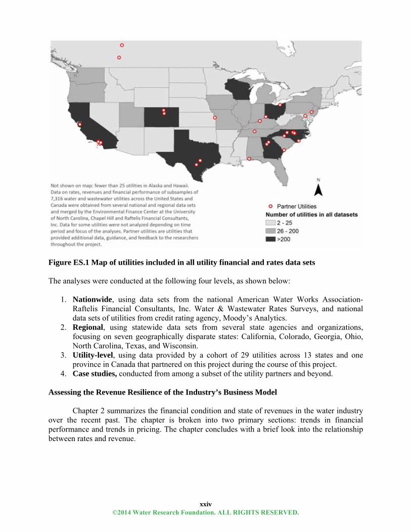
Figure ES.1 Map of utilities included in all utility financial and rates data sets The analyses were conducted at the following four levels, as shown below:
1. Nationwide, using data sets from the national American Water Works Association-
Raftelis Financial Consultants, Inc. Water & Wastewater Rates Surveys, and national data sets of utilities from credit rating agency, Moody’s Analytics.
2. Regional, using statewide data sets from several state agencies and organizations, focusing on seven geographically disparate states: California, Colorado, Georgia, Ohio, North Carolina, Texas, and Wisconsin.
3. Utility-level, using data provided by a cohort of 29 utilities across 13 states and one province in Canada that partnered on this project during the course of this project.
4. Case studies, conducted from among a subset of the utility partners and beyond. Assessing the Revenue Resilience of the Industry’s Business Model
Chapter 2 summarizes the financial condition and state of revenues in the water industry
over the recent past. The chapter is broken into two primary sections: trends in financial performance and trends in pricing. The chapter concludes with a brief look into the relationship between rates and revenue.
©2014 Water Research Foundation. ALL RIGHTS RESERVED.

xxv
Trends in Financial Performance This section analyzes how utilities across North America have fared financially over the
last decade with a focus on the robustness of utility business models in generating stable and adequate revenue streams. Key findings include: For the majority of utilities, the largest component of utility revenues comes from customer
sales (base and variable charges). Generally, variable revenues from a utility’s commodity charges comprise the largest portion of those sales.
As such, operating revenues for many utilities are “bumpy.” Many utilities experience significant year-to-year revenue variability (Figure ES.2).
Figure ES.2 Annual changes to total operating revenues among the same 485 utilities nationwide
Between any given consecutive years between FY2004 and FY2011, revenues decreased for 14% to 37% for a cohort of 485 utilities from across the country.
On a national level and state level, the fastest rise in total operating revenues occurred in the years immediately preceding the 2008 economic downturn. After the economic downturn, revenues continued to rise for the majority of the utilities but at a much slower pace (Table ES.1).
Table ES.1 Average trends in median increases to operating revenues in cohorts of utilities in six
states Fiscal Year: ‘01 ‘02 ‘03 ‘04 ‘05 ‘06 ‘07 ‘08 ‘09 ‘10 ‘11 ‘12
California (n=946) 4.5%/year 2.2%/year
Georgia (n=333) 6.2% 0.1%/year 3.9%/year
North Carolina (n=306) 3.6%/year 5.7%/year 2.8%/year
Ohio (n=400) 1.2%/year
Texas (n=286) 4.7%/year 2.1%/year
Wisconsin (n=567) 2.1%/year 0.8%/year
©2014 Water Research Foundation. ALL RIGHTS RESERVED.
xxvi
While it is clear that operation and maintenance expenses have risen over the past decade, it is important to compare this trend to changes in operating revenues. In 2007 through 2009, operating and maintenance expenses rose faster than operating revenues for more utilities than not. However, that trend reversed itself in 2010, with more utilities experiencing greater increases in operating revenues than in operating and maintenance expenses.
Pricing Trends and Financial Resilience This section highlights national and statewide trends in water and wastewater rates and
rate adjustments, within the context of financial stability. The analysis focuses on trends in rate adjustment frequency and the extent of rate adjustments across regions, over time, and at different consumption levels. It analyzes the trends around fixed versus variable charges and explores what this means for revenue resiliency. The section concludes with a brief look into the relationship between rates and revenue. Key findings include:
Smaller and regular rate increases are associated with higher credit ratings.
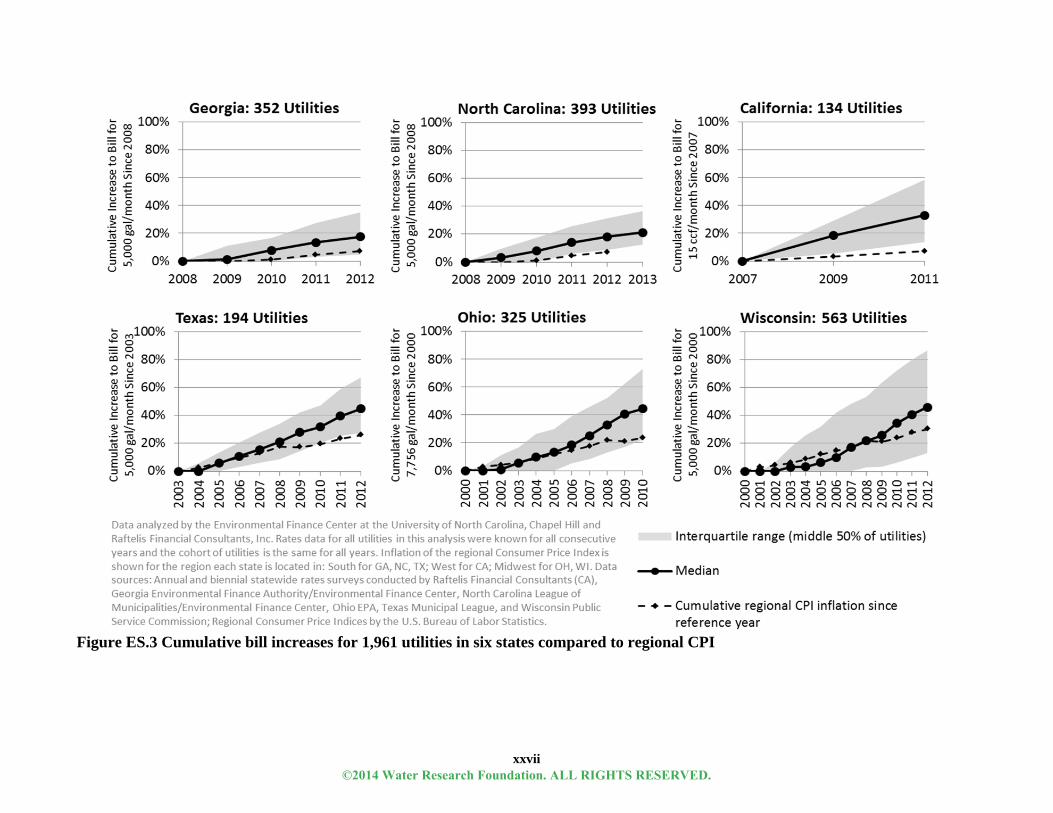
Though the exact size of the cumulative rate increases over time varied from state to state, most utilities increased rates at a pace slightly faster than regional Consumer Price Index (CPI) inflation, particularly after the financial crisis (Figure ES.3). In some states, however, there were also many utilities whose rates failed to keep pace with inflation.
Larger utilities across the country adjusted water rates fairly frequently over the last ten years
at levels that outstripped inflation.
Many utilities have seen revenue generation track behind, and in some cases significantly behind, the percentage they have increased their customers’ rates (Figure ES.4).
©2014 Water Research Foundation. ALL RIGHTS RESERVED.
xxvii
Figure ES.3 Cumulative bill increases for 1,961 utilities in six states compared to regional CPI
©2014 Water Research Foundation. ALL RIGHTS RESERVED.

xxviii
Figure ES.4 Increases in rates and operating revenues for 94 utilities nationwide, 2004 to 2012
Factors Influencing Revenue Resiliency
Chapter 3 considers these trends in the context of factors that influence a utility’s current business model and their ability to implement new practices. Major factors and associated trends include:
Service Area Size & Diversity: Utilities serving a larger customer base tend to have lower
rates and stronger financial performance metrics than their smaller counterparts.
Water Use & Weather: Water use for many utilities is the defining characteristic in revenue health under current pricing and finance models. National trends indicate that average water use per capita and per account is generally decreasing over time.
Economic Conditions: A bad economy, so far, has not resulted in a drastic decline in
aggregate revenues across the industry, but has appeared to slow revenue growth from pre-downturn conditions, potentially resulting in increasing affordability pressure for many utilities.
Capacity Utilization: Utility capacity varies significantly among individual utilities with
many using a relatively small fraction of their system’s capacity during average periods. Economic Regulation & Governance: The economic regulatory framework over a utility
can have a major influence on the types of financial practices it can implement, but economic regulation alone does not necessarily guarantee financial strength or resilience.
Financial Management Strategies: Water and wastewater utilities use a number of
integrated management theories that can be used alone or in concert to further utility financial and management goals.
©2014 Water Research Foundation. ALL RIGHTS RESERVED.

xxix
Credit Rating Agencies: Credit rating agencies serve as both a reflection and driver of utility’s financial performance. Credit rating agencies are analyzing a utility’s preparation and response to the factors outside of its control, with a focus on flexibility, capacity, and predictability (Figure ES.5).
Figure ES.5 Key credit rating considerations of S&P for 18 drinking water utilities from 2010-2012 Strategies and Practices for Revenue Resiliency
Chapter 4 presents a suite of revenue resiliency strategies, policy, and practice options,
including:
Demand Projections: Detailed, integrated, and updated, demand forecasting can help water resource managers and finance officers make plans with more confidence and less financial risk.
Rethinking Utility Services: Many utility managers have begun looking at options beyond selling traditional services to diversify revenues, including the sale of fire protection services.
Alternative Rate Designs: The industry has an opportunity to adopt pricing models that
better align cost-of-water to the cost-of-service (Figure ES.6). The report explores the financial impact of three models on utilities and their customers.
©2014 Water Research Foundation. ALL RIGHTS RESERVED.

xxx
Figure ES.6 Comparison of monthly and annual charges for a customer under a utility’s current rate structure to an alternative rate (PeakSet Base) modeled rates for the same amount of water use
Financial Performance Targets: Financial policies can be used as yardsticks for financial performance; by monitoring financial performance against specified targets, a utility can hold itself accountable for financial stability while maintaining flexibility.
Rate Stabilization Reserves: The types of reserve funds and levels at which utilities keep their reserve funds vary widely, but there are some discernible trends among the project’s partner utilities (Table ES.2). Rate stabilization reserves can mitigate variations in rate increases; and utilities with lower reserve levels (relative to operating expenses and debt service) had more volatile rate increases than those with larger reserve fund ratios.
Table ES.2 Utility Reserve Fund Targets
Utility Reserve Fund TargetsCity of Minneapolis 15% of revenue budget for the next year Orange Water and Sewer Authority The greater of 33% of O&M budget or 20% of the total
estimated cost of the succeeding 3 years of the CIP budget Baltimore Dept. of Public Works Minimum of 90 days cash on hand Alameda County Water District Sufficient to meet operating, capital, and debt service
obligations Charlotte-Mecklenburg Utilities 100% of operating expenses for the current budget Water District No.1 of Johnson County The Board will be notified when the rate stabilization reserve
reaches a minimum level of $2 million
Customer Affordability & Assistance Programs: Keeping rates unsustainably low for all customers at the cost of water and wastewater infrastructure investment benefits no one in the long term. Affordability programs provide flexibility to utilities seeking revenue resiliency.
$‐
$20.00
$40.00
$60.00
$80.00
$100.00
$120.00
July(25)
Aug(21.1)
Sept(14.4)
Oct(9.9)
Nov(7.2)
Dec(7.3)
Jan(8.4)
Feb(6.5)
Mar(6.6)
Apr(11.4)
May(18.7)
June(29.9)
WaterCharge
FiscalYear2011(kgalconsumed)
CurrentRate($647.75)
PeakSetBase($621.55)
Resident1
Ratestructure(annualchargefor
FY10PeakDemand
24,100gallons
©2014 Water Research Foundation. ALL RIGHTS RESERVED.
xxxi
Rate Adjustment Approaches: Alternative processes for raising rates, such as cost-indexed rates, multi-year increases, and pass-through charges, incrementally help quell some of the political and public adversity to rate increases.
Tools to Assist with Revenue Resiliency
This project generated two tools to assist utilities in exploring pricing and program strategies for revenue resiliency. Each tool is explained in more detail below:
Revenue Risk Assessment Tool: This tool allows utilities to quickly determine the
proportion of residential revenues from water sales at risk of loss when demand patterns change, based on the utility's own rate structure, customer demand profile, and weather conditions. The tool requires only minimal data and uses simplifying assumptions based on actual customer behavior. It focuses exclusively on revenue projections and assessments and allows the user to compare two different rate structures and assess which one offers greater revenue resiliency. The Revenue Risk Assessment Tool and accompanying tutorial video are available on the WRF Website on the 4366 project page under Project Resources/Web Tools.
Customer Assistance Program Cost Estimation Tool (CAPCET): This tool was developed to help utilities assess the costs and benefits of implementing a customer affordability program in their service area. Using information from the U.S. Census Bureau and water and wastewater rates inputted by the user, this interactive instrument incorporates information about the eligibility threshold to qualify for an affordability program, annual assistance offered per customer, percent of customers responsible for bad debt, among other fields. By adjusting the appropriate fields, the results provide insight into design considerations and program costs. The CAPCET and accompanying tutorial video are available on the WRF Website on the 4366 project page under Project Resources/Web Tools.
Conclusions and Recommendations
This research reinforces the growing sentiment among many in the industry that the general water utility business and pricing model is not as robust and resilient as once thought. Most water utilities rely on the sale of one essential product, and historically, many utilities have raised sufficient and predictable revenue through small rate modifications. While this approach has never been foolproof, the quantitative analyses throughout this report offer additional evidence that the last five years has been a particularly trying time for this business model.
A resilient business model for the water industry is one that is strategic and deft. Specifically, utilities should:
Understand their business risk for disruptive revenue fluctuations. Adopt basic policies and performance targets to drive financial decisions. Re-examine sales projection methodologies. Consider the repercussions of the message that customers are buying gallons of
water when the cost side of the business model suggests they are buying access to water.
Consider new pricing models.
©2014 Water Research Foundation. ALL RIGHTS RESERVED.

©2014 Water Research Foundation. ALL RIGHTS RESERVED.

1
CHAPTER 1: BACKGROUND AND METHODOLOGY
Introduction It seems like publications across the country are claiming a “new normal” for any number
of cultural or financial trends. College students are financing their education with increasing levels of debt and decreasing salaries, as reported by the New York Times in “A Dangerous ‘New Normal’ in College Debt” (Blow 2013). City managers are bracing for a “new normal” in which tax revenues “can’t be expected to return” (Kavanagh 2013). The term is used to discuss transformative changes in lifestyles, finances, technology, weather, politics, and behavior.
For the water utility industry, the “new normal” has been categorized as a changing climate (Lacey 2011), declining consumption (Rockaway et al. 2011), and a looming capital deficit (AWWA 2012; USEPA 2009). In these early years of the 21st century, utility managers face a delicate balancing act in achieving financial health while facing mounting financial, regulatory, and environmental pressures. Results from the 2012 State of the Water Industry report indicate that U.S. water and wastewater utilities continue to suffer from the impacts of the weak economic recovery and struggle to raise sufficient revenues to cover mounting costs (Murphy 2012).
The large amount of capital needed to address the industry’s aging infrastructure has risen to the forefront of local and national policy discussions over the last five years (AWWA 2012; USEPA 2009; Baird 2010; Haarmeyer 2011; Matichich, Allen, and Allen 2006). In 2013, the American Society of Civil Engineers scored the state of the nation’s drinking water and wastewater systems with a grade of “D” (ASCE 2013). In 2007, the U.S. Environmental Protection Agency (USEPA) estimated approximately $334 billion in infrastructure investment would be needed to simply maintain U.S. water utilities’ existing infrastructure through 2026 (USEPA 2009). A 2012 report by American Water Works Association (AWWA) estimates that projected costs for the sector could exceed $1 trillion by 2035 (AWWA 2012). By any account, the amount of funds needed by the industry remains daunting. In a harrowing wake-up call to communities rallying against water rate increases, the report states,
“In the years ahead, all of us who pay for water service will absorb the cost of this investment, primarily through higher water bills. The amounts will vary depending on community size and geographic region, but in some communities these infrastructure costs alone could triple the size of a typical family’s water bills.” (AWWA 2012) Compounding the impact of rising costs is declining consumption. Recent reports
confirm anecdotal evidence from water utilities around the nation: average household water use has declined steadily since 1995 (DeOreo and Mayer 2012). In another study, when controlling for weather and other variables, a household in the 2008 billing year used nearly 12,000 gallons less annually than an identical household in 1978 (Rockaway et al. 2011). For utilities that collect the majority of the revenues that they need to cover capital costs from charging per unit (whether in gallons, cubic feet, or acre feet) charges, this trend presents a major financial challenge and has led to re-examining the fundamental utility business model.
©2014 Water Research Foundation. ALL RIGHTS RESERVED.

2
An emerging trend in the U.S. water utilities is the paradoxical relationship between customers’ water use efficiency/conservation and water utility revenue. Many water utilities grapple with a conundrum: they encourage customers to use water more efficiently, but maintain pricing models that lead to the loss of significant amounts of revenue when customers reduce their water consumption.
This report examines the impact of the existing business model on financial resiliency: the ability to thrive in the presence of fiscal stresses that threaten to temporarily or systematically move an organization or industry off-balance or out of fiscal equilibrium. Resiliency goes a step beyond sustainability: indicating thriving, rather than just surviving (Cascio 2009).
As the following Focus and Methodology sections discuss in more detail, this report uses a large and unique dataset to conduct a primary exploration of recent financial trends and revenue resiliency. The report does not seek to identify a single treat to resiliency, but rather explores and highlights the variation among utility performance and operating environment. The analysis clearly shows that there is not one generalizable “new normal” or inevitable pre-ordained financial outcome for the industry. There are clearly differences between regions, states, and utilities. The analysis shows that although the prevailing revenue model has posed problems for many utilities, it continues to serve many utilities relatively well.
Most importantly, this report shows there is no single “silver bullet” strategy for revenue resiliency. The strategies chosen introduce practical practices for revenue diversity, redundancy, flexibility, and foresight: some of the key characteristics of a resilient system (Cascio 2009). This report presents examples of current, emerging, and “out of the box” strategies available to utilities to build a resilient business model. Focus
The research in this report provides an assessment of the revenue model and resulting
financial condition of water utilities in North America (primarily the United States), considers factors influencing financial performance, and discusses practices that have the potential to improve financial resiliency. Financial condition is a function of whether revenues collected are balanced with or appropriate to the revenue base, whether revenues are balanced with spending, and whether there is sufficient surplus to account for potential risks (Hendrick 2011). A quick review of any major water conference agenda or research publication will show the abundance of important research going on today looking at the “cost” side of the financial balance utilities must navigate. Entire journals and research events are devoted to important topics such as cost optimization of new treatment technologies or cost mitigation potential of asset management practices. Complementing this cost analysis, this report focuses almost exclusively on the revenue and rates side of the equation.
Figure 1.1 displays a model describing the factors that affect a water utility’s financial condition, adapted from a model described by Hendrick (2011). The bolded statements in the figure summarize the scope of this report. This focus is not meant to discount the importance of balancing revenues and spending and reducing costs appropriately, but rather to emphasize the topic and narrow the scope of the research. Chapter 2 summarizes the financial condition and state of revenues in the water industry. Chapter 3 considers these trends in the context of the factors that influence a utility’s current business model and their ability to implement new practices. Chapter 4 presents revenue resiliency strategy, policy, and practice options. The
©2014 Water Research Foundation. ALL RIGHTS RESERVED.

3
revenue risk assessment tool (RVAT) associated with this project presents a methodology for assessing the risk of revenue losses.
Figure 1.1 This report will focus on financial condition, revenues, and rates (model adapted from Hendrick 2011)
In summary, this report provides a large-scale, quantitative analysis of the financial
reality of water utilities across the country. Case studies and micro-quantitative analysis of a small cohort of utility partners illustrate trends in long-run financial solvency and explore the financial ramifications of various practices. In its entirety, the report serves as a utility financial review, grounded in practical and applied approaches to securing revenue resiliency. It brings together a myriad of datasets and reports to reflect current trends and practices in revenue resiliency. Many of the practices discussed in Chapter 4 of the paper were discussed in the Water Research Foundation’s “Rates and Revenues: Water Utility Leadership Forum of Meeting Revenue Gaps” (Haskins et al. 2011). This report explores the financial implications of those practices in greater detail. Methodology
Both quantitative and qualitative analyses are used in this research. Large, secondary data
sets from multiple organizations were merged to quantitatively assess the state and trends of utility finance and rates across thousands of utilities. Data and information collected from individual utilities were used to qualitatively describe practices in revenue resiliency in the water industry in more depth. While this research seeks to identify specific trends and practices, it is also an important goal for this research to highlight the variations and diversity of practices and financial conditions across water utilities.
External Features: Constraints, Opportunities, Responsibilities, and
Demands
Internal Policy Choices
Revenues Pricing and Rates
Spending Pressures (and obligations) Spending
Financial Condition
Determination of Service Levels
©2014 Water Research Foundation. ALL RIGHTS RESERVED.

4
The analyses were conducted at the following four levels, as shown in Figure 1.2:
5. Nationwide, using data sets from the national American Water Works Association-Raftelis Financial Consultants, Inc. Water & Wastewater Rates Surveys, and national data sets of utilities from credit rating agency, Moody’s Analytics.
6. Regional, using statewide data sets from several state agencies and organizations, focusing on seven geographically disparate states: California, Colorado, Georgia, Ohio, North Carolina, Texas, and Wisconsin.
7. Utility-level, using data provided by a cohort of 29 utilities across 13 states and one province in Canada that partnered on this project during the course of this project.
8. Case studies conducted from among a subset of the utility partners and beyond.
Figure 1.2 Four levels of data analysis in this report
Each step used to collect, clean and analyze data for this research is described below. Data identification
In order to assess the state of and trends in water utility finance across North America, large national data sets were identified that could track the relationship between utility business and pricing models and utility financial performance over several years for the same set of utilities (at least as a subsample of the full data set). In addition, to assess and highlight varying conditions across the country and between utilities, similar data sets focused on one state or one region were identified. A list of data needs for data sets to be considered as part of this research was specified, including data on utilities’ operating revenues, operating expenses, and customer charges (rates) for at least one consumption point.
Many agencies and organizations across the country collect financial and rates data on water utilities for a number of reasons: to regulate, to assess creditworthiness, or to provide a service to the utilities. For example, some state funding agencies collect financial data from the audited income statements of local government utilities to monitor their ability to pay back state loans. Others monitor utilities’ abilities to pay back any loan. Some private organizations collect information on utility charges to provide a benchmarking service.
Qualitative analysis
Nationaldatasets
Statewidedatasets
Cohortofutilitypartners
CaseStudies
Quantitative analysis
©2014 Water Research Foundation. ALL RIGHTS RESERVED.
5
Numerous national and regional data sets were identified for initial consideration by: 1) past experience creating, working with and knowledge of existing data sets on water utility finance and rates, 2) a thorough internet search for all water rates surveys conducted across the United States, and 3) reviewing the websites of various state agencies that may have a reason to collect water utility financial or rates data from a large number of utilities, such as Offices of State Treasurers/Controllers, utilities commissions, and state funding agencies.
The initial list was then narrowed down to those that provided data for more than 100 water utilities either across the United States or within one state or region, carried out over several years since 2000, included a large subsample of utilities for which data were available in every survey year, and contained at least some of the data requirements. Next, the list of statewide data to be used in this analysis was further narrowed by: 1) identifying states for which utility financial performance and utility rates data were available, even if in different data sets, and 2) preferring states that were geographically disparate and that had different regulatory environments, climates, socioeconomic conditions, and/or customer water use patterns.
Ultimately, for utility financial and rates data, two large national datasets and data from seven states were chosen and used in this analysis. The data sets included data on utilities in all 50 states and a few in Canada, as shown in Figure 1.3. The data sets are described in Table 1.1.
Utility financial data was integrated with data on factors that may contribute to the financial performance of utilities. Examples include local income levels and poverty rates obtained from the U.S. Census Bureau’s American Community Surveys, county unemployment rate from the U.S. Bureau of Labor Statistics, and local drought conditions from the U.S. Drought Monitor.
This research was done in partnership with a diverse group of utilities from across North America. These “partner utilities” provided guidance as well as information that was used to carryout utility-specific research. Partner utilities received targeted analyses and the ability to participate in peer-to-peer exchanges on the research and with other partner utilities. The 29 partner utilities, listed below, were spread across North America in 13 states and one province in Canada as shown in Figure 1.3. The partner utilities were:
Alameda County Water District, CA Aqua America, Inc. (nationwide, but headquartered in PA) Austin Water Utility, TX Beaufort-Jasper Water and Sewer Authority, SC Cape Fear Public Utility Authority, NC Charlotte-Mecklenburg Utilities Department, NC City of Baltimore Department of Public Works, MD City of Calgary Water Services, Alberta, Canada City of Durham Department of Water Management, NC City of Loveland Department of Water and Power, CO City of Raleigh Public Utilities Department, NC Clayton County Water Authority, GA Daphne Utilities, AL Davidson Water, Inc., NC Denver Water, CO EPCOR Utilities, Inc., (Edmonton), Alberta, Canada
©2014 Water Research Foundation. ALL RIGHTS RESERVED.
6
Glendale Water and Power, CA Gwinnett County Department of Water Resources, GA Louisville Water Company, KY Mesa Consolidated Water District, CA Metropolitan Sewer District of Greater Cincinnati, OH Metropolitan Water District of Southern California, CA Nashville Metro Water Services, TN Northeast Ohio Regional Sewer District, OH Orange Water and Sewer Authority, NC San Antonio Water System, TX Town of Cary Public Works and Utilities Department, NC Water District No.1 of Johnson County, KS Yorba Linda Water District, CA
©2014 Water Research Foundation. ALL RIGHTS RESERVED.
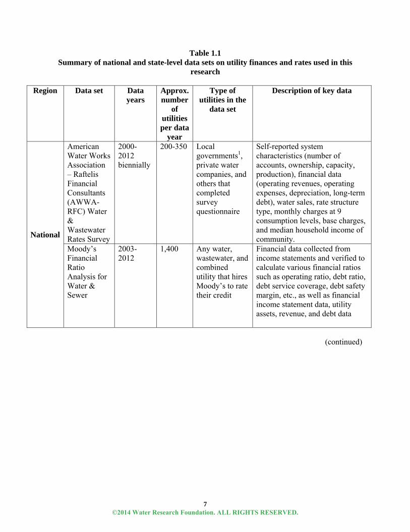
7
Table 1.1 Summary of national and state-level data sets on utility finances and rates used in this
research
Region Data set Data years
Approx. number
of utilities per data
year
Type of utilities in the
data set
Description of key data
National
American Water Works Association – Raftelis Financial Consultants (AWWA-RFC) Water & Wastewater Rates Survey
2000-2012 biennially
200-350 Local governments1, private water companies, and others that completed survey questionnaire
Self-reported system characteristics (number of accounts, ownership, capacity, production), financial data (operating revenues, operating expenses, depreciation, long-term debt), water sales, rate structure type, monthly charges at 9 consumption levels, base charges, and median household income of community.
Moody’s Financial Ratio Analysis for Water & Sewer
2003-2012
1,400 Any water, wastewater, and combined utility that hires Moody’s to rate their credit
Financial data collected from income statements and verified to calculate various financial ratios such as operating ratio, debt ratio, debt service coverage, debt safety margin, etc., as well as financial income statement data, utility assets, revenue, and debt data
(continued)
©2014 Water Research Foundation. ALL RIGHTS RESERVED.

8
Table 1.1 (Continued) Region Data set Data
years Approx. number
of utilities per data
year
Type of utilities in the data set
Description of key data
California
CA State Controller’s Office Special Districts Annual Report
FY2001- FY2010 annually
1,190 Special districts (local governments excluding municipalities or counties)
Self-reported financial data provided by county auditors and special district officials, including operating and non-operating revenues and expenses, broken down by customer class and source, depreciation, long-term debt, taxes, etc.
Raftelis Financial Consultants and CA-NV Section of American Water Works Association (RFC-CA/NV AWWA) Water Rate Survey
2005-2011 biennially
216-358 since 2007
Local governments and private water companies that completed survey questionnaire
Self-reported rate structure type, billing frequency, base charge, commodity charge and total charge at 15 ccf/month charge, service population, average residential water use, connection fees. A sub-set of these utilities in 2009 and 2011 submitted detailed rate structure data that were used to compute monthly water charges for 0 – 15,000 gallons of water use at 1,000 gallon intervals.
Colorado
CO Water Resources and Power Development Authority (CWRPDA) internal database
2003-2010 annually
150-250 Local governments that have outstanding loans or bonds with CWRPDA
Terms and details of loans/bonds, total revenues, revenues from tap fees, operating expenses, depreciation, debt service, current assets, current liabilities, debt service coverage ratio and other indicators used by CWRPDA in assessing utility’s financial condition.
(continued)
©2014 Water Research Foundation. ALL RIGHTS RESERVED.

9
Table 1.1 (Continued)
Region Data set Data years
Approx. number of utilities per data year
Type of utilities in the data set
Description of key data
Georgia
GA Department of Community Affairs Report of Local Government Finances & Report of Registered Authority Finances
FY2006-FY2011 annually
500-640 Local governments (municipalities, counties and authorities)
Self-reported financial data including operating revenues, operating expenses, depreciation, debt service payments, and total long-term debt remaining.
Georgia Environmental Finance Authority and Environmental Finance Center at the University of North Carolina, Chapel Hill (GEFA/EFC) Water & Wastewater Rates Survey
2007-2012 annually
415-475 Local governments (municipalities, counties, and authorities)
Compiled and verified rate structures, base charges, and detailed rate structure data used to compute monthly water and wastewater charges for 0 – 15,000 gallons at 1,000 gallon intervals, for customers inside and outside town limits (if applicable).
(continued)
©2014 Water Research Foundation. ALL RIGHTS RESERVED.

10
Table 1.1 (Continued)
Region Data set Data years
Approx. number of utilities per data year
Type of utilities in the data set
Description of key data
Ohio
OH Water Development Agency (OWDA) internal database
2006-2010 annually
320-715 Local governments that have outstanding debt with OWDA
Gross revenues, operations and maintenance expenses, total expenses, debt service, debt, number of customers by type, median household income and poverty rate, history and degree of rate increases.
OH Environmental Protection Agency (Ohio EPA) Sewer and Water Rate Survey
1999-2010 annually
475-550 Local governments
Self-reported water and wastewater residential charges for 7,756 gallons/month, and tap-in fees for residential customers.
(continued)
©2014 Water Research Foundation. ALL RIGHTS RESERVED.

11
Table 1.1 (Continued)
Region Data set Data years
Approx. number
of utilities per data
year
Type of utilities in
the data set
Description of key data
North Carolina
NC Local Government Commission internal database compiled from audited financial statements data
FY1997-FY2012 annually
425-515 Local governments
Financial data obtained from financial statements including operating revenues, operating expenses, depreciation, debt service payments, assets, liabilities, unrestricted cash and investments, total long-term debt remaining, etc.
NC League of Municipalities and Environmental Finance Center at the University of North Carolina, Chapel Hill (NCLM/EFC) Water & Wastewater Rates Survey
1986, 2000, 2002, 2005-2013 annually
330-507 since 2005
Local governments, non-profit associations and for-profit water companies (since 2012)
Compiled and verified rate structures, base charges, and detailed rate structure data used to compute monthly water and wastewater charges for 0 – 15,000 gallons at 1,000 gallon intervals, for customers inside and outside town limits (if applicable).
NC Dep’t of Environment and Natural Resources’ Division of Water Resources Local Water Supply Plans
1997, 2002, 2007-2011 annually
470-540 water systems
Local government water systems and large community water systems
Self-reported data on water systems’ permitted treatment capacity, maximum and average daily withdrawals/discharges for 12 months, production, water use (sales) by customer type, and number of metered connections by customer type.
(continued)
©2014 Water Research Foundation. ALL RIGHTS RESERVED.
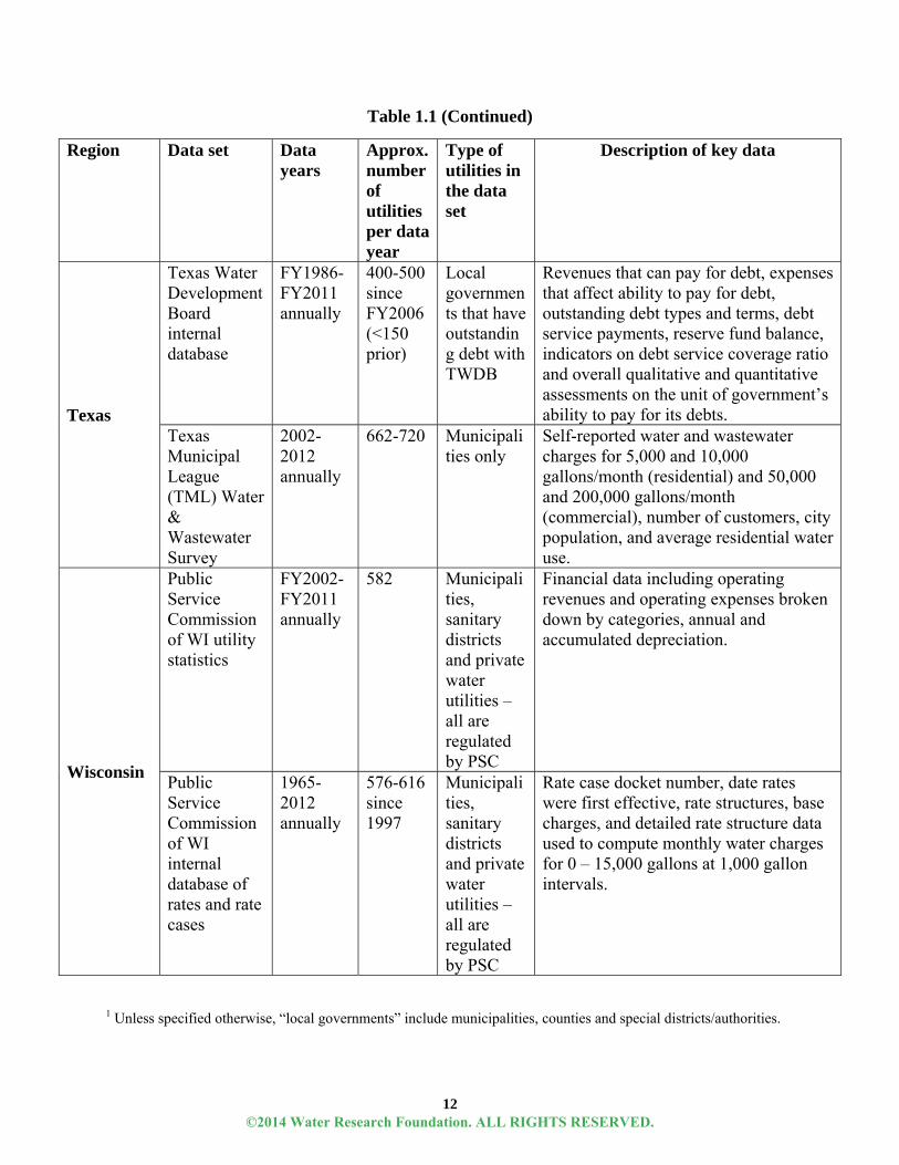
12
Table 1.1 (Continued)
1 Unless specified otherwise, “local governments” include municipalities, counties and special districts/authorities.
Region Data set Data years
Approx. number of utilities per data year
Type of utilities in the data set
Description of key data
Texas
Texas Water Development Board internal database
FY1986-FY2011 annually
400-500 since FY2006 (<150 prior)
Local governments that have outstanding debt with TWDB
Revenues that can pay for debt, expenses that affect ability to pay for debt, outstanding debt types and terms, debt service payments, reserve fund balance, indicators on debt service coverage ratio and overall qualitative and quantitative assessments on the unit of government’s ability to pay for its debts.
Texas Municipal League (TML) Water & Wastewater Survey
2002-2012 annually
662-720 Municipalities only
Self-reported water and wastewater charges for 5,000 and 10,000 gallons/month (residential) and 50,000 and 200,000 gallons/month (commercial), number of customers, city population, and average residential water use.
Wisconsin
Public Service Commission of WI utility statistics
FY2002-FY2011 annually
582 Municipalities, sanitary districts and private water utilities – all are regulated by PSC
Financial data including operating revenues and operating expenses broken down by categories, annual and accumulated depreciation.
Public Service Commission of WI internal database of rates and rate cases
1965-2012 annually
576-616 since 1997
Municipalities, sanitary districts and private water utilities – all are regulated by PSC
Rate case docket number, date rates were first effective, rate structures, base charges, and detailed rate structure data used to compute monthly water charges for 0 – 15,000 gallons at 1,000 gallon intervals.
©2014 Water Research Foundation. ALL RIGHTS RESERVED.

13
Figure 1.3 Map of utilities included in all utility financial and rates data sets Data collection, cleaning, and preparation
The data sets were collected from their sources either by downloading from websites,
contacting and requesting the data directly from their sources, or compiling existing data. If questionnaires were used to collect the data, a copy of the questionnaire was also obtained.
For the most part, the organizations that compiled these data sets work in isolation of one another and focus exclusively on their individual objectives and client base when they collect, clean, and publish their data. As such, the collection of water utility data across the country is not uniform. Even the methods of data collection are not uniform. Many organizations favor surveys in the form of questionnaires that places reporting onus on the utilities themselves, with little follow-up or data verification occurring by the researching organization. Surveys that rely on self-reporting by utilities, by nature, introduce errors since many people, in various positions at the utilities responding to the survey, may read and interpret the same questionnaire question differently. In other cases, particularly among credit rating agencies and state regulatory agencies, utilities submit audited documents to the organization that then combs through the documents to extract data in a standard manner. In this case, data compilation may be more uniform at the research organization level, but the data reported in the original documents may have been compiled slightly differently across the utilities. For example, definitions of financial measurements were not standardized across the data sets shown in Table 1.1, despite Government Accounting Standard Board requirements for public systems, and neither were the financial metrics or ratios.
©2014 Water Research Foundation. ALL RIGHTS RESERVED.
14
For these reasons, a significant amount of time was spent reviewing and cleaning the data. The original data were reviewed for completeness and to understand how the data in each field was calculated or obtained. Comparisons were made across datasets and data fields were standardized whenever possible, or new fields were created and calculated from existing data. Missing or erroneous values were either replaced when obvious (e.g.: correcting a wrong decimal place placement) or the observation was dropped entirely if the data were determined to be questionable or incomplete for key data requirements. In some cases, the original large data sets were whittled down to a smaller data set based on data quality, validity, and completeness.
Next, data were compiled into one large relational database that combined all of the data from the data sets listed in Table 1.1. To do this, every unique water and/or wastewater utility for which data were available in at least one data set and in at least one data year were identified. The database is continuously being updated and as of April 2013, contained an inventory of 7,316 unique utilities in all 50 states, Washington D.C. and several provinces in Canada. Each utility was matched to at least one county or municipality based on its service area. The relational database was compiled to include all of the cleaned data from the different data sets, with relational tables that link all of the original data to one utility from this inventory of unique utilities.
In many cases, this report brings together data sets that have not been compared to one another. The analysis focuses on summary and descriptive statistics. Although there are thousands of contextual stories behind the data, the compilation and comparison of raw numbers tells its own story. Instead, to highlight financial context, data were also compiled from the cohort of partner utilities that represent geographical and organizational diversity. Rate schedules, comprehensive annual financial reports (CAFRs), budgets, rates models, newspaper articles, financial policies, bond covenants, and other planning documents were requested, for several consecutive years. Most utilities provided at least some of these data; the web was also a resource. The rate schedules were used to compute the residential charges for 0 – 15,000 gallons/month at 1,000 gallon intervals. A separate spreadsheet was compiled using the quantitative data obtained from these documents. During the writing of case studies, staff members at the partner utilities were interviewed. The selection and discussion of the strategies and practices for revenue resiliency arose largely from discussion with staff members from these utilities.
Finally, a literature review was conducted in conjunction with the data collection and analysis, to supplement the research findings. A wide range of literature from the fields of public administration, water industry, environmental, and energy industry research was surveyed to supplement the analysis on financial conditions, context, and strategies. Quantitative analysis
Data across data sets were standardized in order to allow computations and comparisons across utilities in the different data sets. For example, when assessing trends in revenues compared to operating and maintenance costs alone, a metric called the “non-capital operating ratio” was defined as the total operating revenues divided by operating and maintenance expenditures. In some financial data sets, operating and maintenance expenditures were reported directly, while in other financial data sets they were computed as total operating expenses minus depreciation, if known. Calculations and definitions similar to this are described in the footnotes of figures throughout this report.
©2014 Water Research Foundation. ALL RIGHTS RESERVED.

15
Some data sets contained more than one observation for each utility in a given data year. For example, some utilities have multiple rate structures, and therefore may have multiple observations in their rates data set. During quantitative analyses, the data were filtered to contain only one (the most relevant) observation per utility in a given data year, unless otherwise specified. Quantitative analyses focused mostly since 2000. Particular attention was paid to changes in trends post-2008, when the economic recession began and possibly may have affected utility finances.
In analyzing trends in rates over time, changes to the monthly bill at a single consumption point was used in this report, unless otherwise noted. The single consumption point for residential rates analyses, dictated by data availability, was chosen to be 5,000 gallons/month in almost all rates data sets, 7,756 gallons/month in the Ohio EPA Sewer and Water Rates Survey, 15 ccf/month (11,220 gallons/month) in the California rates data set, and 10 ccf/month (7,480 gallons/month) in the AWWA-RFC Water and Wastewater Rates Surveys. Where water and wastewater rates were known in all years of analysis, the combined monthly bill was used for analysis, otherwise the water monthly bill was used.
When analyzing how revenues or rates changed over time nationwide or statewide, the change in each utility’s revenues or rates was computed first before calculating the median or interquartile ranges of changes across the country or state. In other words, the median or average bill or revenues in one year’s sample was never calculated and compared to the median or average bill or revenues in another year’s sample, since the sample of utilities varied every year. Instead, only the utilities that were present in both years were used in the analysis, and the reported statistics reflect the median or interquartile range of changes that occurred at the utility-level statewide or nationwide. In some cases, where noted, a single cohort of utilities that had data available for every single year of analysis was used to report trends. The results section and the footnotes in the graphs indicate whether the analysis was using a single cohort of utilities for which data were known in every year, or was using varying samples of utilities for which data were known in two years for which changes were computed. Generally speaking, line graphs were used when the analysis included a cohort of utilities for which data were known in every year and bar charts otherwise.
Quantitative analysis of partner utility data followed the same techniques listed above. The analysis using partner utility data focused more on demonstrating the diversity of trends across even a small number of utilities. Furthermore, the additional data provided by the partner utilities allowed for a quantitative assessment of utility finances and rates in much more detail and depth than is possible using national or regional data sets. For example, analysis on short-term fixed versus variable revenues and costs was only possible using partner utility data, since larger data sets do not typically collect such information. Qualitative analysis
When partner utility data were used to demonstrate the diversity of trends across a small number of utilities, context was provided by speaking with utility staff members, and from newspaper articles and published reports. Similarly, information from utility staff, utility websites, and published reports were used to write up case studies and examples of particular financial practices and strategies implemented by some of the partner utilities.
©2014 Water Research Foundation. ALL RIGHTS RESERVED.
16
Communication and feedback from practitioners
Throughout this research, partner utility staff and water industry experts were updated on the research findings, and invited and encouraged to provide feedback and advice to help guide the direction of the research. The experts included those on the Project Advisory Committee, as well as others working in utilities, research organizations, funding agencies, credit rating agencies, technical assistance providers, and state and federal agencies. The research was presented at numerous national and state conferences and workshops, always showing the latest analyses and findings. Many of these presentations included an interactive component, allowing participants to share their thoughts and opinions in real time that were then incorporated into the report. For example, at the 2012 AWWA Annual Conference and Exposition, a panel of expert utility industry “judges” and more than 30 members in the audience rated four revenue resiliency strategies. Partner utility staff members participated in five virtual discussions in “peer-to-peer exchanges.” These peer-to-peer exchanges provided opportunities to present preliminary results, new decision-making and benchmarking tools created for the partner utilities specifically, and most importantly, to exchange dialogue between the partner utilities on the topic at hand. Finally, a blog, called “Environmental Finance” available at http://efc.web.unc.edu/, was created during this project. Blog posts were written frequently, presenting the latest analyses and results, examples and case studies of financial practices and strategies, new concepts in utility finance, and to share available resources for water utilities. Staff members from some of the partner utilities also contributed their own blog posts. The partner utilities and the Project Advisory Committee were notified when new blog posts were posted (approximately every other week), and invited to share their feedback in the comments section.
References ASCE (American Society of Civil Engineers). 2013. 2013 Report Card for America’s
Infrastructure. Reston, Va.: ASCE. [Online]. Available: <http://www.infrastructurereportcard.org/> [cited May 31, 2013]
AWWA (American Water Works Association). 2012. Buried No Longer: Confronting America’s Water Infrastructure Challenge. Denver, Colo.: AWWA.
Baird, G.M. 2010. A Game Plan for Aging Water Infrastructure. Jour. AWWA, 102(4):74-82. Blow, C. 2013. A Dangerous ‘New Normal’ in College Debt. New York Times, March 8.
[Online] Available: <http://www.nytimes.com/2013/03/09/opinion/blow-a-dangerous-new-normal-in-college-debt.html?_r=0> [cited May 31, 2013]
Cascio, J. 2009. The Next Big Thing: Resilience. Foreign Policy Magazine, April 15. [Online]. Available:
<http://www.foreignpolicy.com/articles/2009/04/15/the_next_big_thing_resilience> [cited May 31, 2013]
DeOreo, W.B. and P.W. Mayer. 2012. Insights into Declining Single-Family Residential Water Demand. Jour. AWWA, 104(6): 383–394.
USEPA (United States Environmental Protection Agency). 2009 Drinking Water Infrastructure Needs Survey and Assessment: Fourth Report to Congress. Washington D.C.: USEPA.
Harmer, D. 2011. A Fresh Look at U.S. Water and Wastewater Infrastructure: The Commercial and Environmentally Sustainable Path Forward. Journal of Applied Corporate Finance, 23(3): 41–52.
©2014 Water Research Foundation. ALL RIGHTS RESERVED.

17
Haskins, S., M. Tiger and J. Hughes. 2011. Rates and Revenues: Water Utility Leadership Forum on Challenges of Meeting Revenue Gaps, Web Report #4405. Denver, Colo.: Water Research Foundation.
Hendrick, R. 2011. Managing The Fiscal Metropolis: The Financial Policies, Practices, and Health of Suburban Municipalities. Washington D.C.: Georgetown University Press.
Kavanagh, S. 2013. Building a Financially Resilient Government through Long-Term Financial Planning. White Paper. Chicago, Ill.: GFOA. [Online]. Available: <http://gfoa.org/downloads/financiallyresilientgovernment_whitepaper.pdf> [cited May 31, 2013]
Lacey, M. 2011. Inside Insight – Say Good-bye to ‘Business as Usual.’ Jour. AWWA, 103(6): 2. Matichich, M., J. Allen, and R. Allen. 2006. Asset Management Planning and Reporting Options
for Water Utilities. Jour. AWWA, 98(1):80–87. Murphy, M. 2012. 2012 State of the Water Industry Report -- An industry at the crossroads.
Jour. AWWA, 104(6):44–57. Rockaway, T.D., P.A. Coomes, J. Rivard and B. Kornstein. 2011. Residential water use trends in
North America. Jour. AWWA, 103(2): 76-89.
©2014 Water Research Foundation. ALL RIGHTS RESERVED.

©2014 Water Research Foundation. ALL RIGHTS RESERVED.

19
CHAPTER 2: ASSESSING THE REVENUE RESILIENCE OF THE INDUSTRY’S
BUSINESS MODEL
TRENDS IN FINANCIAL PERFORMANCE
Introduction
The majority of water and wastewater utilities in North America are organized to be
financially self-sufficient, such that revenues collected by the utility from its customers should cover all of the expenses incurred, without the need to obtain additional revenue from taxes, other enterprises, or other organizations. Utilities have significant control over setting rates, fees, penalties and various charges (sometimes pending regulatory approvals); in theory, they have financial autonomy. This rate setting autonomy does not directly translate to revenue autonomy. Financial performance is influenced by many more factors than rates and charges and is explored throughout various sections of this report. In fact, even before the United States experienced a major economic downturn, stories were beginning to appear on the fiscal challenges facing utilities. The term “gap” was often used in these accounts to describe the business status of the water utility industry with many policy analyses focusing on large aggregated estimations of capital needs or funding shortfalls (USEPA 2002).
This chapter analyzes how utilities across North America have fared financially over the last decade with a focus on the robustness of the utility business model in generating stable and adequate revenue streams. The analysis relies on multiple national, state, and individual utility-level data sets, compiled over a wide range of data sources. Almost all of the original data originated from the audited financial statements of utilities, and have been compiled by various agencies and organizations. Utilities self-reported financial data from their audited income statements in the biennial national American Water Works Association-Raftelis Financial Consultants, Inc. (AWWA-RFC) Water and Wastewater Rate Surveys since 2000.1 Other national data was compiled from the Moody’s Municipal Financial Ratio Analysis database, which contains debt and other financial data, as well as credit rating and calculated financial metrics for utilities nationwide. These national data are analyzed to detect trends in utility revenues and expenses since 2000.
In order to analyze differences in trends across regions with differing regulatory, economic, and weather climates, separate historic data for hundreds of utilities from seven disparate states were also analyzed. The seven states are: California, Colorado, Georgia, North Carolina, Ohio, Texas, and Wisconsin. The original financial data were compiled by different agencies and organizations in slightly different ways and for different purposes in these states. Data sets were compiled and common measures identified that can be compared across states and
1 The sample of utilities included in this national data set included a disproportionately greater percentage of larger water utilities than the actual national average. Therefore, trends detected from this national data set better represent trends observed by larger utilities than smaller ones.
©2014 Water Research Foundation. ALL RIGHTS RESERVED.

20
across time to be analyzed in this chapter. The statewide data sets include a greater number of smaller water utilities than the national data sets.
Finally, annual audited financial statements for 26 partner utilities spread across the United States and Canada were collected and financial data extracted for ten years (FY2002 – FY2011) where available. A more thorough description of the data and methodologies used in analyses is included in the Background and Methodology section of this report.
Key Points
The largest component of utility revenues comes from customer sales. Generally, variable
revenues from a utility’s commodity charges comprise the largest portion of those sales. In the last 10 to 12 years, most utilities have experienced an overall growth in total
operating revenues, with utilities generally collecting more revenues now than at any time in that period (not adjusting for inflation).
On a national level and state level, the fastest rise in total operating revenues occurred in the years immediately preceding the 2008 economic downturn. After the economic downturn, revenues continued to rise for the majority of the utilities but at a much slower pace.
The Business Model Behind Utility Revenues
Utilities collect revenues from multiple sources, including charges to customers, fees, and
grants (AWWA 2012). Water and wastewater utility revenues are divided into operating revenues and non-operating revenues. Operating revenues are revenues derived from the various operations of the water system, including revenues from the sale of water and discharge of wastewater for all customers; connection (tap) fees linked to actual installation costs (as opposed to system development charges to cover system capacity); customer fees and penalties assessed for account changes, disconnections and reconnections, late payments; ad valorem taxes; power generation sales; rents from water system property; and all other revenues that are incidental to water operations (AWWA 2012). Non-operating revenues are revenues that do not derive from the operations of the water system itself, including interest and dividends on investments; revenues from system development charges or capacity fees; rents from nonutility property; and provision of services to other organizations (AWWA 2012). Investor-owned utilities report their operating and non-operating revenues in annual reports to their shareholders, and local government-owned utilities typically report their financial performance in an audited Income Statement following guidance set by the Governmental Accounting Standards Board. All income statements contain data on utilities’ operating revenues, operating expenses (primarily expenses for operations and maintenance, plus depreciation and amortization), and non-operating revenues and expenses (capital expenditures and/or debt service payments).
©2014 Water Research Foundation. ALL RIGHTS RESERVED.

21
Figure 2.1 Total operating revenues as a percent of total revenues among 662 utilities nationwide in 2012
In particular, sales to customers based on water use and wastewater discharge – revenues derived from the monthly water and wastewater charges including commodity (usage) charge revenues and revenues from the fixed monthly service charges – is the single most significant source of revenue for utilities. As shown in Figure 2.2, customer sales typically comprise over 90% of a utility’s total operating revenues, with the remainder being derived from fees, penalties, connection (tap) charges, rents, and power generation.
0%
10%
20%
30%
40%
50%
60%
70%
80%
90%
100%
Upto75% 76‐80% 81‐85% 86‐90% 91‐95% 96‐100%
Percen
t of U
tilities
Total Operating Revenues as a Percent of Total RevenuesDataanalyzedbytheEnvironmental FinanceCenterattheUniversityofNorthCarolina,ChapelHillandRaftelisFinancialConsultants,Inc.DataSource:Moody'sWaterandSewerMunicipalFinancialRatioAnalysis.
©2014 Water Research Foundation. ALL RIGHTS RESERVED.

22
Figure 2.2 Revenues from customer sales as percent of total operating revenues in FY2011
Customer sales can be divided into two general categories: fixed revenues that are not dependent on a customer’s water use or wastewater discharge, such as the revenues obtained from the monthly base charges, and variable revenues that are explicitly linked to the volume of water used or wastewater discharged by the customers, derived from the volumetric charges. The balance between fixed revenues and variable revenues is unique for each utility, based on rate structure design, pricing levels, and base charges, and on the water demand of the customer base.
Unfortunately, data on variable revenues and fixed revenues from customer sales are not included in most large sample datasets, but was available from data collected from individual utilities. However, many utilities on an individual level are just beginning to monitor this. These layers of utility revenues are illustrated in Figure 2.3 for two such utilities: Water District Number 1 of Johnson County, KS (WaterOne) and the Alameda County Water District, CA. Commodity charges accounted for 76% and 61% of total revenues for the two utilities, respectively.
©2014 Water Research Foundation. ALL RIGHTS RESERVED.

23
Figure 2.3 Layers of revenues and the proportion of revenues from commodity charges in two utilities
Table 2.1 shows a breakdown between variable and fixed revenue for a group of utilities
from different regions of the country. In most cases, the majority of customer sales are obtained from the commodity charges. In fact, between 71% and 96% of the customer sales revenues collected by these nine utilities were obtained from the commodity charges. While these percentages are representative for many utilities in North America, particularly for large utilities, other utilities may have lower variable revenue percentages if they set high base charges and lower volumetric charges. The City of Durham, NC, demonstrates such a trend towards decreasing variability. At the beginning of Fiscal Year 2009, Durham nearly doubled its base charges and only slightly increased its volumetric rates. As a consequence, the proportion of single-family residential customer sales revenues that were obtained from the commodity charges fell from 82% to 71% between FY2008 and FY2009, as more of the revenue came from the base charges. The Charlotte-Mecklenburg Utilities Department (NC) also sought to increase the proportion of fixed revenues from customer sales by increasing the base charges for its customers in FY2012 and estimated in their budget projections that the variable revenues portion would drop from 95% to 84% in FY2012.
©2014 Water Research Foundation. ALL RIGHTS RESERVED.

24
Table 2.1 Proportion of customer sales (base charges + commodity charges)
collected from commodity charges
Utility
Fiscal Year
2007 2008 2009 2010 2011 2012
budget estimates
Utilities reporting proportions of revenues from all customers* Alameda County Water District, CA 88% Charlotte-Mecklenburg Utilities, NC 95% 96% 95% 84%Louisville, KY 80% 77% 78% 79% 77% Mesa Consolidated Water District, CA 74% 76% 76% 75% WaterOne (Johnson County), KS 80% 77% 73% 76% 78% Utilities reporting proportions of revenues from single-family residential customers only** Cary, NC 91% 91% 90% 91% 92% Durham, NC 82% 82% 71% 74% 72%
Raleigh, NC 76% 75% 75% 75% 78% Data Sources: * Reported by the utility. Revenues from all customers included. ** Billing records of all single-family residential customers analyzed by the Environmental Finance Center at the University of North Carolina, Chapel Hill, and FY2011 results were estimated based on a partial year of records.
By nature, variable revenue is more vulnerable to fluctuations from year-to-year. For example, WaterOne reported “wetter than normal years” in FY2008 and FY2009 and lower than normal water use (14% and 18% less than in FY2007, respectively). During wet years, customers often use less water outdoors for lawn irrigation and other activities. For WaterOne, this resulted in a decline in variable revenue, despite the fact that volumetric rates increased. This illustrative example demonstrates the vulnerability of the largest component of customer sales (the commodity charges), which is the largest component of customer sales and operating revenues, which are the largest components of total revenues for the utility, to factors that may be beyond the control of the utility.
It is important to note two important factors that some utilities weigh heavily in recovering less operating revenue through the fixed charges. First, high fixed service charges can be regressive, as they result in higher unit costs for low-volume users, some of whom may be low-income customers. Second, higher fixed charges translate to lower commodity (usage) rates, which can reduce the conservation pricing signals associated with the commodity charges. National Trends in Total Operating Revenues
As stated earlier, although a telling indicator of financial stability, this level of detail is
not typically collected in financial surveys. As such, the following analysis looks at trends in operating revenues with the understanding that North American utilities have similar models to the previously highlighted examples. Moody’s rating agency evaluates thousands of utilities each year and has compiled financial and debt data for these utilities. Although the sample of rated utilities was much larger, a subset of these utilities (485) was analyzed to portray a “snapshot” of finance trends across all states over the last decade. The annual change in total operating revenues between years from 2004 to 2011 was computed for each utility.
©2014 Water Research Foundation. ALL RIGHTS RESERVED.
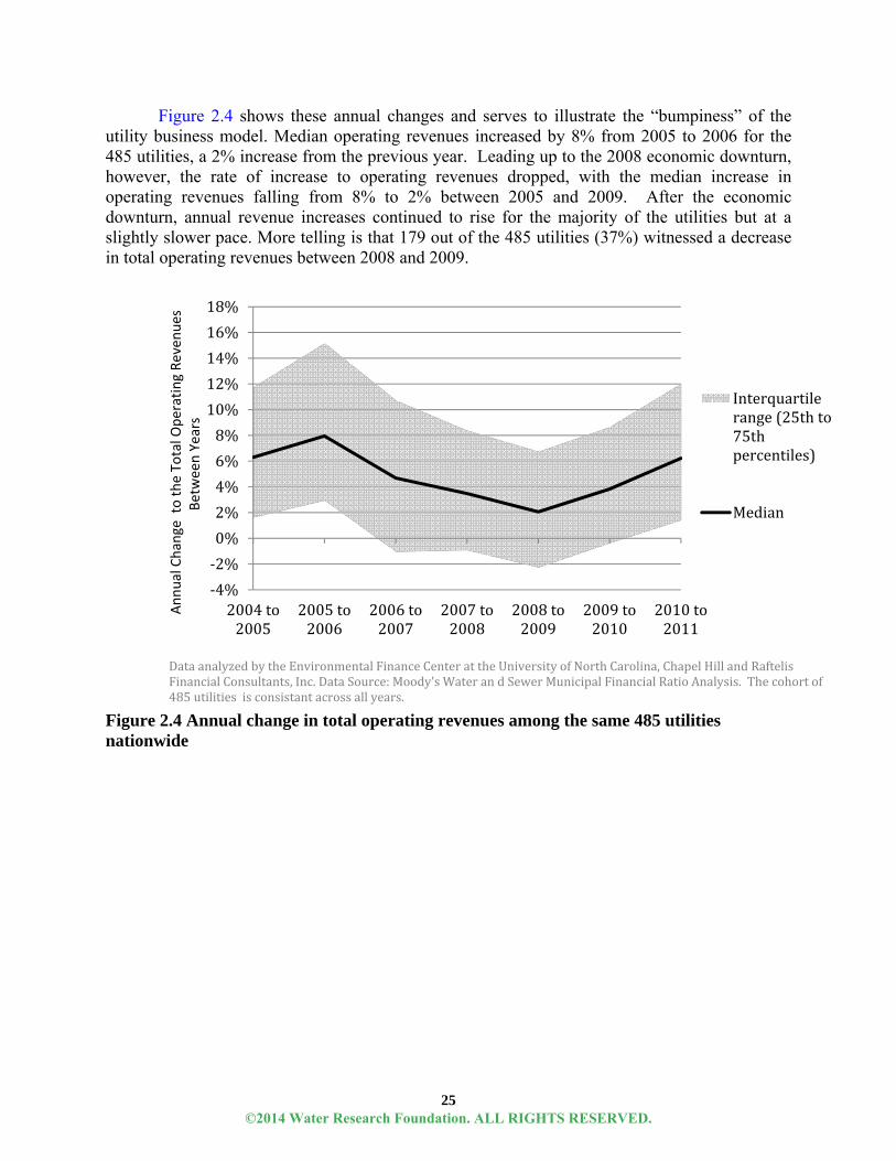
25
Figure 2.4 shows these annual changes and serves to illustrate the “bumpiness” of the utility business model. Median operating revenues increased by 8% from 2005 to 2006 for the 485 utilities, a 2% increase from the previous year. Leading up to the 2008 economic downturn, however, the rate of increase to operating revenues dropped, with the median increase in operating revenues falling from 8% to 2% between 2005 and 2009. After the economic downturn, annual revenue increases continued to rise for the majority of the utilities but at a slightly slower pace. More telling is that 179 out of the 485 utilities (37%) witnessed a decrease in total operating revenues between 2008 and 2009.
Figure 2.4 Annual change in total operating revenues among the same 485 utilities nationwide
‐4%
‐2%
0%
2%
4%
6%
8%
10%
12%
14%
16%
18%
2004to2005
2005to2006
2006to2007
2007to2008
2008to2009
2009to2010
2010to2011
Annual Change to the To
tal O
perating Reven
ues
Between Years
Interquartilerange(25thto75thpercentiles)
Median
DataanalyzedbytheEnvironmental FinanceCenterattheUniversityofNorthCarolina,ChapelHillandRaftelisFinancialConsultants,Inc.DataSource:Moody'sWaterandSewerMunicipalFinancialRatioAnalysis.Thecohortof485utilitiesisconsistantacrossallyears.
©2014 Water Research Foundation. ALL RIGHTS RESERVED.

26
Statewide Trends in Total Operating Revenues Trends in total operation revenues were analyzed for larger samples of utilities over
longer periods of time from data collected by state agencies. For this project, financial data for local government water and wastewater utilities were obtained from state agencies in California, Colorado, Georgia, North Carolina, Ohio, Texas, and Wisconsin. These seven states are geographically spread across the United States and reflect varied approaches to utility financial management, as explained in the Background and Methodology section. For example, unlike in the other states, local government utilities in the State of Wisconsin are financially regulated by a Public Service Commission and require state approval for rate increases. In other states, like North Carolina and Georgia, the majority of local government utilities only require the approval of a single local governing body to raise rates.
Figure 2.5 summarizes trends in revenues, particularly operating revenues, between Fiscal Years 2000 – 2012 for a cohort of 2,838 utilities in six states. Changes to the operating revenues from one year to the next were computed for the utilities with data in every single year of analysis for that state. For example, in California, the median change in total operating revenues among 946 special districts between FY2001 and FY2002 was + 4.5%. Between FY2009 and FY2010, the median change was an increase of 2.2% for the same cohort of 946 special districts.
©2014 Water Research Foundation. ALL RIGHTS RESERVED.
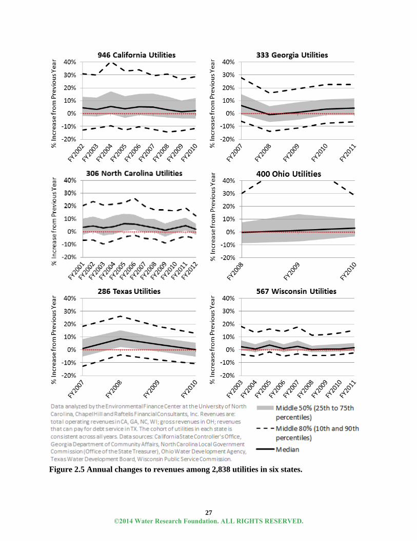
27
Figure 2.5 Annual changes to revenues among 2,838 utilities in six states.
©2014 Water Research Foundation. ALL RIGHTS RESERVED.

28
In all six states, the median change to operating revenues from one year to the next was greater than or equal to zero. This indicates that, from year-to-year in the past decade, operating revenues for at least half of the utilities increased, despite a downturn in the economy, severe weather fluctuations, and general declines to customer water use patterns. Since operating and capital costs increase for most utilities over time (seeTrends in Utility Expenses following section on Trends in Utility Expenses), this trend is critical to utility financial health.
However, the rate of increase to utilities’ revenues has not been consistent over this time period. In particular, utilities’ revenue increases slowed down in the later years of the decade. Table 2.2 summarizes how the revenue increases changed over time by displaying the average of the median revenue increases for the cohorts of utilities for different periods of time in each state. Blocks of time are shaded to indicate the degree of revenue increases. (Time periods with no data are blacked-out in the table.) As shown in Table 2.2 and in Figure 2.5, the median rate of revenue increases at least halved after FY2008 for nearly all states. More than half of the utilities in California, Georgia, North Carolina, and Texas were enjoying at least a 4.5% annual growth to their revenues prior to FY2008, but saw their revenue increases slow down after FY2008.
Table 2.2 Average trends in median increases to operating revenues in cohorts of utilities in six states
Fiscal Year: ‘01 ‘02 ‘03 ‘04 ‘05 ‘06 ‘07 ‘08 ‘09 ‘10 ‘11 ‘12
California (n=946) 4.5%/year 2.2%/year
Georgia (n=333) 6.2% 0.1%/year 3.9%/year North Carolina (n=306)
3.6%/year 5.7%/year 2.8%/year
Ohio (n=400) 1.2%/year
Texas (n=286) 4.7%/year 2.1%/year
Wisconsin (n=567) 2.1%/year 0.8%/year
Examples of Utilities’ Trends in Total Operating Revenues
To bring the analysis down to an individual utility level, data from project utility partners
was compiled and analyzed in Table 2.3. Nearly all of the 18 utilities, spread across the United States and Canada, had steadily increasing total operating revenues in the past ten years but there was a substantial variation in magnitude. For example, in FY2010, total operating revenues for Metro Water Service’s (in Nashville, Tennessee) were only 29% greater than they were in FY2002. On the other hand, Aqua America, Inc. and its subsidiaries nationwide managed to increase its annual operating revenues by 134% in the same time period. This resulted from a combination of steady rate increases in order to achieve an acceptable and Utilities Commission-approved rate of return for Aqua America’s shareholders, and increasing the number of customers by 60% in those ten years, which is a higher-than-normal growth rate for this past decade. By contrast, the Metro Water District’s customer base increased by only 7% between FY2006 and FY2011, and the utility raised rates only in the last two of those six years.
©2014 Water Research Foundation. ALL RIGHTS RESERVED.

29
Table 2.3 Trends in total operating revenues in 18 utilities, FY2002-FY2011
Many of the utilities witnessed at least one year of low or negative growth to their total
operating revenues between FY2007 and FY2010. For example, Gwinnett County, GA’s total operating revenues decreased by 6% in FY2008, amidst otherwise steady increases between FY2002 and FY2011. In this case, Gwinnett County’s retail and wholesale customers used 18% less water in 2008 than they did in 2007, possibly as a result of a severe drought in combination with the economic downturn. However, this was not the only time that Gwinnett County’s customers used less water than in the previous year. Between 2002 and 2010, average daily demand dropped in four of the eight years, albeit at much smaller rates. Yet, Gwinnett County’s total operating revenues increased every year except in FY2008. Gwinnett County was able to achieve this result by steadily increasing its volumetric rates every year, more than compensating for the decreases in demand except in FY2008. In fact, Gwinnett County did not raise its base charges except in FY2010, demonstrating that a utility can overcome demand and customer declines by setting rates that take into account significant usage declines.
Trends in Utility Expenses
Similar to revenues, all expenses of water and wastewater utilities are divided into operating expenses and non-operating expenses. Operating expenses are expenses that apply to
'03 '04 '05 '06 '07 '08 '09 '10 '11Alameda County Water District, CA 1.46Aqua America Inc. 2.34Beaufort-Jasper Water & Sewer Authority, SC 2.08City of Calgary Water ServicesClayton County Water Authority, GA 1.59Charlotte-Mecklenburg Utilities, NCDavidson Water, Inc., NC 1.28EPCOR Utilities Inc. (Edmonton)Gwinnett County, GA 1.69WaterOne (Johnson County), KSLouisville, KYLoveland, COMesa Consolidated Water District, CA 1.49Metropolitan Water District of Southern California 1.22Nashville, TN 1.29NEORSD, OHSan Antonio, TX 1.78Yorba Linda, CA 1.96
Relative Gain or Loss in Total Operating Revenues from
Previous Year (Fiscal Year)
Ratio of Total Operating
Revenues in FY2011 to
FY2002
Total Operating Revenues(FY2002 - FY2011)
Data analyzed by the EnvironmentalFinance Center at the University of North Carolina, Chapel Hill and Raftelis Financial
Consultants, Inc. Data Source: Income Statements and Comprehensive Annual Financial Reports. Bars reflect the percent change to total operating revenues from previous fiscal year. Dark bars are relative gains, light bars are relative losses. The y‐axis scales are unique for each utility.
©2014 Water Research Foundation. ALL RIGHTS RESERVED.

30
the provision of water utility services, including operation expenses (expenses incurred in operating and administering the water system and customer service), maintenance expenses for day-to-day repairs (excluding rehabilitation and replacement of current capital assets), depreciation expenses, and amortization expenses (AWWA 2012). Non-operating expenses are all other expenses that do not apply to the provision of water services, such as interest payments on debt, net loss on disposal of assets, lawsuit expenses, property taxes, etc. (AWWA 2012). Key Points
In general, operating expenses constitute the majority of all expenses for utilities, including the somewhat intangible cost of current asset depreciation and amortization.
For most utilities, fixed costs by far exceed their variable costs for utilities, particularly when debt service payments and other capital expenditures are included in the calculation.
Operation and maintenance expenses increased rapidly between 2004 and 2012, much like national trends in total operating revenues. The median annualized increase in operation and maintenance expenses dropped from +5.8% per year between 2004 and 2010 to +1.0% per year between 2010 and 2012.
Prior to 2012, expenses were generally rising faster than operating revenues. Only recently (between 2010 and 2012) did the trend reverse.
Sixteen percent of utilities had operating ratios less than 1.0 as reported in 2004, growing each subsequent survey year to 28% in 2010 before returning to 16% in 2012.
The gap between revenues and expenses varies from state to state, painting a unique picture of trends in financial sufficiency in each state.
Utility Expenses Deconstructed
In general, operating expenses (which includes operating expenditures and depreciation and amortization of current assets) constitute the majority of all expenses for utilities, as shown in Figure 2.6. For the same utilities, the distribution of operating expenses to total expenses is more varied than the operating revenues to total revenues shown in Figure 2.1. Among 260 utilities in 45 states surveyed in the 2012 AWWA-RFC Water & Wastewater Rate Survey, operating expenses accounted for more than 80% of total expenses for 72% of utilities.
©2014 Water Research Foundation. ALL RIGHTS RESERVED.

31
Figure 2.6 Total operating expenses as a percent of total expenses among 260 utilities nationwide
And although, they are the primary focus of this report, revenues only tell half of the business model’s story. Utilities, funding agencies, and credit rating agencies typically compare utilities’ revenues to expenses to assess the business strength of a utility. Different organizations use different metrics, but most are founded on the belief that utilities are a capital intensive business in which operating revenue is expected to cover both cash operating expenditures (labor, fuel, chemicals etc.) as well as capital related expenses (debt service or in some cases depreciation). For example, Fitch Ratings calculates the debt service coverage ratio as the division of “revenues available for debt service” by the debt service for the year (Fitch Ratings 2012). Revenues available for debt service include the operating revenues less cash expenditures (i.e.: operation expenses). This calculation is more intuitive and critical, since it tracks actual expenditures and assesses the utility’s ability to make its payments during the course of the year. However, not all utilities incur debt, and those that do may not be borrowing the full amount needed to rehabilitate or replace all of their assets. Instead, utilities usually employ a mix of borrowing and paying cash for capital infrastructure projects.
Just as it is important to understand the balance between stable “fixed” revenue streams and highly variable revenue streams, it is important to assess the same distinction on the expense side. Operation and maintenance expenses (operating expenses minus debt service payment and depreciation) include both short-term fixed and short-term variable costs. Short-term variable expenses are the costs that are directly related to the amount of water or wastewater processed, treated, delivered, and/or discharged. These include the costs for bulk water purchases, chemicals, power, and some other materials. Short-term fixed expenses are costs that do not vary in the short-term based on water demand. Fixed expenses include labor, billing and meter reading, transportation, insurance, rent, contracts, employee benefits, repair of equipment, and
©2014 Water Research Foundation. ALL RIGHTS RESERVED.

32
most materials. Some of these costs may be variable in the long-term, but in the short-term, these would not be immediately affected by daily, or even yearly, fluctuations to customer water use demands.
For most utilities, fixed costs by far exceed their variable costs for utilities, particularly when debt service payments and other capital expenditures are included in the calculation. However it is difficult to quantitatively assess this trend because centralized data on variable and fixed expenses are not readily available within large datasets and are difficult to readily extract from Comprehensive Annual Financial Reports. Figure 2.7 displays the utility-calculated fixed versus variable costs for two utilities in different regions of the country to demonstrate the business challenge facing many utilities. Alameda County Water District’s costs are pulled from their operating budget; no depreciation and capital expenses are included. Austin’s costs represent their total anticipated expenses for FY2012, including capital costs. The costs and expenses should not be compared between the utilities, but rather within. In both cases, more than 87% of expenses were determined to be fixed. Conversely, fixed revenues from customer sales account for only a small portion of total customer sales; less than 17% in these two examples. The consequence of relying on variable revenues to pay what are primarily fixed expenses at the utility, with customer demand fluctuations, are significant and are highlighted and discussed throughout this report.
Figure 2.7 Fixed versus variable costs and revenues for two utilities
©2014 Water Research Foundation. ALL RIGHTS RESERVED.

33
Figure 2.8 shows another representation of the nature of utility costs. As the figure shows, for the 126 utilities included in Moody’s database, a significant portion of utilities revenues are devoted to debt service payments each year; costs that are completely independent of the amount of water services provided to customers. Figure 2.8 highlights trends in a significant relatively fixed cost for many water utilities: debt. It is important to note that these trends are found in utilities rated by Moody’s, which are those that are issuing debt.
Figure 2.8 Debt service as a percentage of total operating revenues for 126 water and combined utilities from 2003-2012 National Trends in Operating Expenses, Relative to Operating Revenues
Operation and maintenance expenses increased rapidly for the majority of utilities
between 2006 and 2012, much like national trends in total operating revenues, according to the data collected by Moody’s rating agency. These expenses consistently rose for most of the utilities in the 517-utility sample throughout the decade, shown in Figure 2.9. However, the median annualized increase in operation and maintenance expenses fell from +4.2% per year between 2006 and 2012 to +2.8% per year between 2011 and 2012. Thus, while operation and maintenance expenses were increasing, the rate of increase fell after 2006. Conversely, average annual increases to total operating revenues remained generally higher than average annual increases to operation and maintenance expenses.
10%
15%
20%
25%
30%
35%
40%
2003 2004 2005 2006 2007 2008 2009 2010 2011 2012
Deb
t Service Paymen
ts as a Percent of To
tal
Operating Reven
ue
Year
Middle50%ofUtilities
Median
Dataanalyzed bytheEnvironmentalFinanceCenterattheUniversityofNorthCarolina,ChapelHillandRaftelisFinancialConsultants,Inc.Datasource:Moody'sratingagency.Thesamegroupofutilitiesisusedeachyear,andonlyutiliteswithdebtdataavailableforalltenyearswereused.
©2014 Water Research Foundation. ALL RIGHTS RESERVED.

34
Figure 2.9 Total operating revenues and operation and maintenance expenses reported in 2012 compared to prior years among 517 utilities nationwide.
Figure 2.10 shows that the percentage of utilities with operation and maintenance expenses rising faster than operating revenues remained between 40 and 50 percent from 2004 to 2008. From 2009 to 2012, however, these percentages fell, indicating an overall increase in the number of utilities with operating revenues rising faster than operation and maintenance expenses. The percentage of utilities where operating revenues and operation and maintenance expenses rose at about the same rate remained fairly constant throughout the years--between 8% and 12%.
‐10%
‐5%
0%
5%
10%
15%
2006to2012
2007to2012
2008to2012
2009to2012
2010to2012
2011to2012
Average Annual Increase (or Decrease) From
Referen
ce Year to 2012
TotalOperatingRevenues(dark:middle50%,light:middle80%)
O&MExpenses(dark:middle50%,light:middle80%)
DataanalyzedbytheEnvironmental FinanceCenterattheUniversityofNorthCarolina,ChapelHillandRaftelisFinancialConsultants,Inc.DataSource:Moody'sWaterandSewerMunicipalFinancialRatioAnalysis.Thecohortof517utilitiesisconsistantacrossallyears.
©2014 Water Research Foundation. ALL RIGHTS RESERVED.

35
Figure 2.10 Comparing annual changes to operating revenues and operation and maintenance expenses in the same 383 utilities nationwide
Comparing revenues to expenses by tracking an “operating ratio” provides additional
insight into the robustness of a utilities business model. Different analysts and organizations may calculate operating ratio differently depending on available data and the purpose of the analysis. The most important and common variation in how this critical metric is calculated relates to whether depreciation is included as an operating expense in the calculation. When depreciation is included, this metric takes into consideration some aspect of a utility’s capital cost and the metric can be seen as cost recovery indicator. In other words, do operating charges generate enough revenue to cover both operation and maintenance expenses, as well as the cost of replacing current capital assets? When depreciation figures were readily available, they were incorporated into our operating ratio calculations. However, depreciation figures were not available in all of the data sets analyzed. If the ratio of total operating revenues divided by operation and maintenance expenses alone is used(not including depreciation and amortization), the metric is labeled as “non-capital operating ratio.”
The non-capital operating ratio shows whether a utility collected sufficient operating revenues (mostly customer sales charges) to pay for day-to-day operations and maintenance expenses alone. In other words, did the utility collect enough revenue from customer charges to pay its bills to run the system, excluding all considerations of capital costs? Of importance to note: neither of these ratios includes debt service or cash payments for capital projects. Figure 2.11 shows trends in non-operating rations for a cohort of 383utilities nationwide. Consistently over 90% of these utilities have been collecting enough revenues to cover their non-capital operating expenses.
0%
10%
20%
30%
40%
50%
60%
70%
80%
90%
100%
2004‐2005
2005‐2006
2006‐2007
2007‐2008
2008‐2009
2009‐2010
2010‐2011
2011‐2012
PercentofUtilities
O&Mexpensesrosefasterthanoperatingrevenues
OperatingrevenuesandO&MexpensesroseataboutthesamerateOperatingrevenuesrosefasterthanO&Mexpenses
DataanalyzedbytheEnvironmental FinanceCenterattheUniversityofNorthCarolina,ChapelHillandRaftelisFinancialConsultants,Inc.DataSource:Moody'sWaterandSewerMunicipalFinancialRatioAnalysis.Thecohortof583utilitiesisconsistantacrossallyears.IncreasesofoperatingrevenuesandO&Mexpenseswithin+‐1%areputinthe"samerate"category.
©2014 Water Research Foundation. ALL RIGHTS RESERVED.

36
Figure 2.11 Non-capital operating ratios for the same 383 utilities nationwide
Figure 2.12 displays the range of operating ratios (including capital expenses) for a national group of utilities that has some, but not complete, overlap with those included in Figure 2.11. Sixteen percent of utilities had operating ratios less than 1.0 as reported in 2004, growing each subsequent survey year to 28% in 2010 before returning to 16% in 2012. These utilities, while mostly able to recover their operation and maintenance expenses through operating revenues, did not collect sufficient operating revenues to also cover their depreciation expenses.
While the median ratios always remained above 1.0, they decreased every survey year between 2004 and 2010, before going up in 2012. In 2004, the median operating ratio was 1.17, indicating that half of the utilities collected enough operating revenues to pay for more than 117% of O&M and depreciation expenses. However, by 2010, the median operating ratio was 1.12. Additionally, all ranges of shifted downwards between 2006 and 2010. Trends in operating ratios began to shift upward between 2010 and 2012. In fact, more utilities had higher ratios in 2012 than in any of the other survey years.
0.00
0.50
1.00
1.50
2.00
2.50
3.00
3.50
2004 2005 2006 2007 2008 2009 2010 2011 2012
OperatingRevenues/O&MExpenses
ReportingYear
Middle80%ofutilities(linesindicateminimumandmaximum)
Middle50%ofutilities(withmedianshownasahorizontalline)
DataanalyzedbytheEnvironmental FinanceCenterattheUniversityofNorthCarolina,ChapelHillandRaftelisFinancialConsultants,Inc.DataSource:Moody'sWaterandSewerMunicipalFinancialRatioAnalysis.Thecohortof583utilitiesisconsistantacrossallyears.
©2014 Water Research Foundation. ALL RIGHTS RESERVED.

37
Figure 2.12 Operating ratios for 529 utilities nationwide Statewide Trends in Operating Expenses, Relative to Operating Revenues
Expanding the analysis to include larger samples of utilities using data from six states emphasizes the magnitude of the decline in financial stability towards the end of the decade and the partial recovery after 2010. The analysis for Ohio, Texas, and Wisconsin includes operation and maintenance expenses only (no depreciation), while the analysis for California, Georgia, and North Carolina include total operating expenses. Differences in the availability of certain expenses data in each state account for the two types of comparisons. The analysis focused on utilities common to every reporting year; the utility sample size for total operating revenue data is reported within each figure.
The utilities’ operating revenues are compared to their operating expenses or operation and maintenance expenses by computing their operating ratios or non-capital operating ratios, respectively. Figures 2.13 and 2.14 track the median and range of the sample of utilities with data in every single year of analysis for that state. For example, the same 946 utilities in California were analyzed for every fiscal year between 2001 and 2010, revealing trends of changing ratios over time throughout the state.
The differences in the two figures demonstrate some variability in financial performance of utilities in different states and may reflect differences in utility governance. As expected, non-capital operating ratios in OH, TX, and WI (Figure 2.14) are generally greater than operating ratios in CA, GA, and NC (Figure 2.13), since depreciation is not included in the analysis for non-capital operating ratios.
©2014 Water Research Foundation. ALL RIGHTS RESERVED.
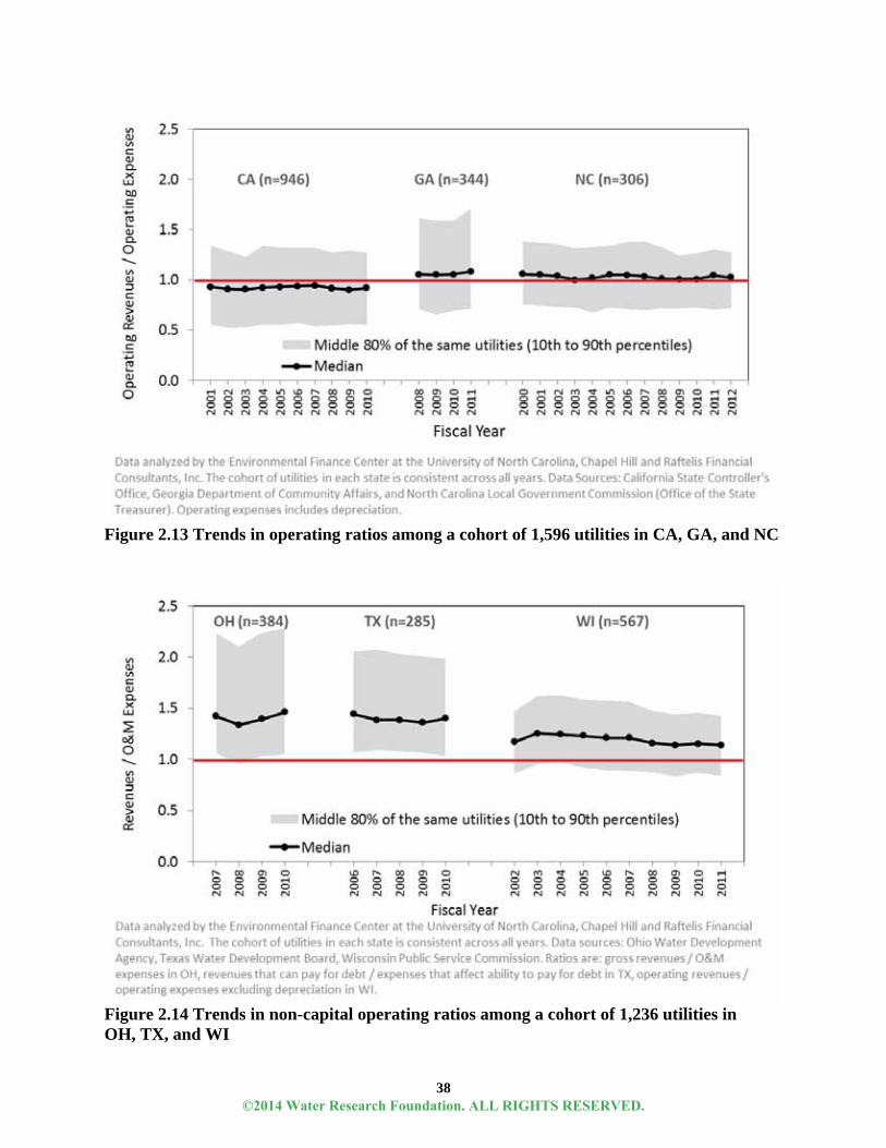
38
Figure 2.13 Trends in operating ratios among a cohort of 1,596 utilities in CA, GA, and NC
Figure 2.14 Trends in non-capital operating ratios among a cohort of 1,236 utilities in OH, TX, and WI
©2014 Water Research Foundation. ALL RIGHTS RESERVED.

39
California had the lowest operating ratios, and is the only state where the median operating ratio was below 1.0. Between FY2001 – FY2010, more than half of the 946 California special districts in this analysis had greater operating expenses, including depreciation, than operating revenues, also shown in Figure 2.5. Ironically, California utilities also saw some of the largest increases in total operating revenues, as shown in Figure 2.5, Annual changes to revenues among 2,838 utilities in six states.
This confirms the earlier observation that operating expenses have grown at a faster rate than operating revenues in California. Georgia’s and North Carolina’s medians hovered just above 1.0.
The three states with data on non-capital operating ratios, in Figure 2.14, consistently had median ratios greater than 1.0. In fact, fewer than 10% of utilities in Ohio and Texas in any year of analysis had lower operating revenues than operation and maintenance expenses, shown in Figure 2.18. This may not be reflective of the utilities throughout those two states, however. The ratios computed in Ohio and Texas were for utilities that had outstanding loans with the Ohio Water Development Agency and the Texas Water Development Board, respectively. These utilities have their financial data reviewed, analyzed and monitored by these two agencies, who work to ensure that the utilities are in strong financial position to pay back their outstanding debts. Hence, there is potential for selection bias in this analysis for these two states, and the utilities included in this analysis may not be representative of all other utilities in Ohio and Texas that do not have this additional factor influencing their financial performance.
By contrast, the ratios computed in Wisconsin were for all public water utilities, which are regulated by the Wisconsin Public Service Commission. This agency, too, reviews, analyzes, and monitors the financial performance of utilities under its purview. The sample of utilities analyzed for Wisconsin is much larger in size than in Ohio and Texas, and better represent the conditions throughout the state. In Wisconsin, between 12% and 26% of utilities, in any given fiscal year, had lower operating revenues than operation and maintenance expenses, as shown in Figure 2.16. Under this type of situation, these utilities would have to use their reserves, transfers, and/or non-operating revenues to fill the gap between day-to-day operations and maintenance expenses and their operating revenues, leaving little to no revenue to cover capital expenses.
The trends in the values of ratios in Figures 2.13 and 2.14, and the percentages of utilities with ratios lower than 1.0 shown in Figures 2.15 and 2.16 indicate that utilities in several states across the country experienced financial difficulties from FY2008 to FY2010, with some continuing into FY2012. In those years, operating ratios and non-capital operating ratios declined in general in CA, NC, TX, and WI, and were low in some of these years for GA and OH. However, the financial performance of utilities in those years was not significantly worse than in prior years. In CA, NC, and WI – the three states with longer time series of data – the financial performance of utilities between FY2008 and FY2010 was similar to the financial performance of the same utilities between FY2002 and FY2004. Thus, although utilities in geographically disperse areas and under different governance structures across the country experienced lower operating ratios and additional strains on finances towards the end of the decade, these difficulties were similar to those experienced in the beginning of the decade.
©2014 Water Research Foundation. ALL RIGHTS RESERVED.
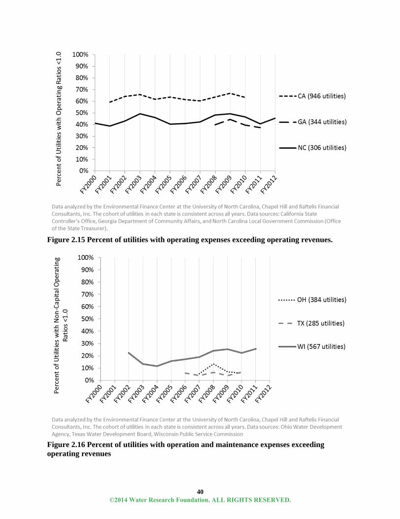
40
Figure 2.15 Percent of utilities with operating expenses exceeding operating revenues.
Figure 2.16 Percent of utilities with operation and maintenance expenses exceeding operating revenues
©2014 Water Research Foundation. ALL RIGHTS RESERVED.

41
Trends in Debt and Debt Service Coverage
Another approach to studying the balance between revenue and costs is to study debt and the amount of cushion utilities that debt-incurring utilities have for covering the repayment of that debt. Figures 2.17 and 2.18, below indicate that utilities are taking on more debt than they have in previous years. Figure 2.17 shows a fairly steady increase in the amount of long term debt per utility from 2003 to 2012 with a larger spread of debt within the middle fifty percent of utilities.
Figure 2.17 Long-term debt for 192 water and combined utilities from 2003-2012
Contrary to trends in long-term debt, national trends in debt service coverage ratios have not risen in a linear fashion. Moody’s calculated the total annual debt service coverage by dividing net revenues by the total annual debt service, including senior and subordinate lien obligations. From 2003 to 2012, median debt service coverage ratios tended to fluctuate between 1.5 and 2.0 for 126 nationwide utilities (Figure 2.18). These ratios dipped significantly from 2008 to 2009, possibly due to the economic recession. While median debt service coverage ratios have been recovering since then, the spread of these ratios among the middle 50% of utilities has decreased.
©2014 Water Research Foundation. ALL RIGHTS RESERVED.

42
Figure 2.18 Debt service coverage ratio for 126 water and combined utilities from 2003 – 2012
How does this influence utilities’ access to the debt market? Figure 2.19 shows a very clear trend of decreasing trend in ratios with credit rating. Out of 18 Aaa rated utilities, the median ratio was 3.6 (with the 80th percentile spanning from 1.3 to 7.3). Out of 50 Aa1 rated utilities, the median ratio dropped to 2.3. Median ratios for A1 rated utilities dropped further to 1.9.
1.00
1.50
2.00
2.50
3.00
2003 2004 2005 2006 2007 2008 2009 2010 2011 2012
DebtServiceCoverageRatio
Year
Middle50%ofUtilities
Median
Dataanalyzed bytheEnvironmentalFinanceCenterattheUniversityofNorthCarolina,ChapelHillandRaftelisFinancialConsultants,Inc.Datasource:Moody'sratingagency.Thesamegroupofutilitiesisusedeachyear,andonlyutiliteswithdebtdataavailableforalltenyearswereused.
©2014 Water Research Foundation. ALL RIGHTS RESERVED.
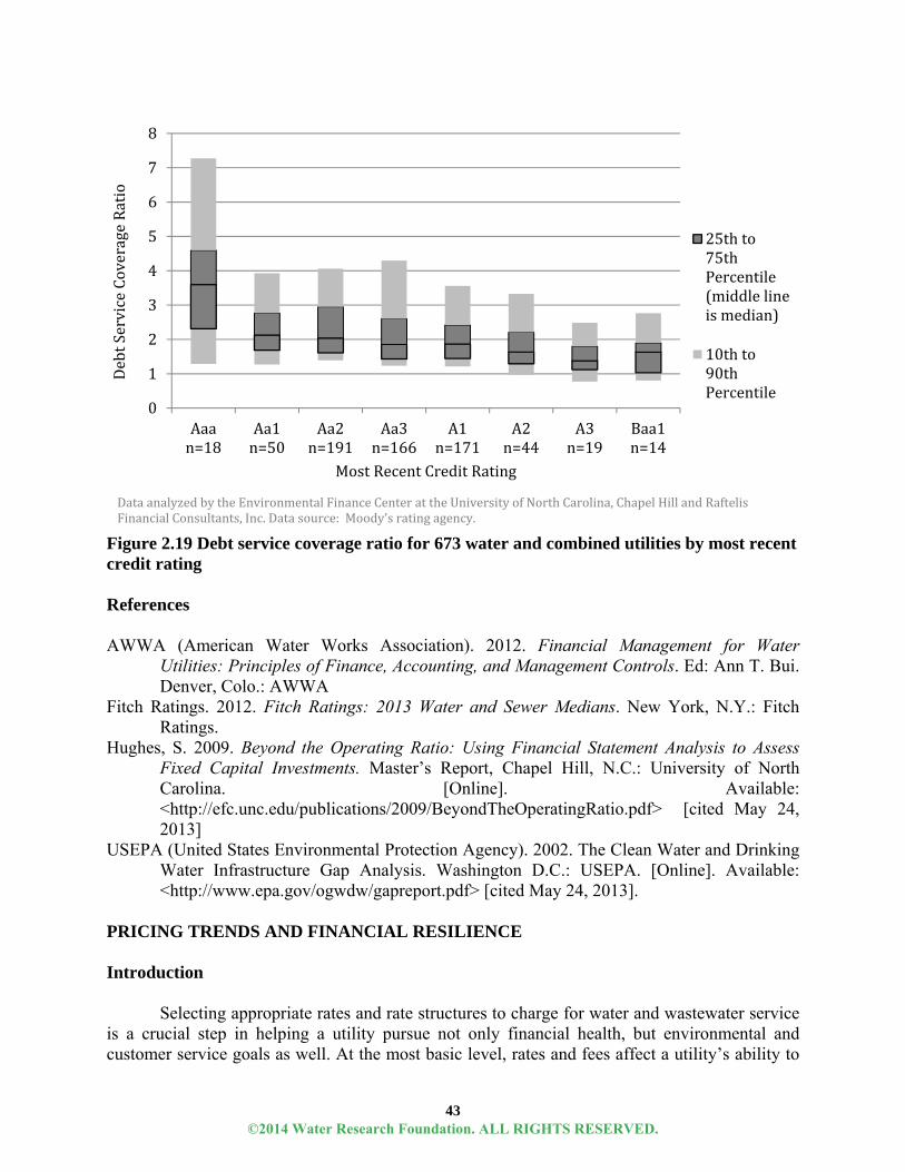
43
Figure 2.19 Debt service coverage ratio for 673 water and combined utilities by most recent credit rating References AWWA (American Water Works Association). 2012. Financial Management for Water
Utilities: Principles of Finance, Accounting, and Management Controls. Ed: Ann T. Bui. Denver, Colo.: AWWA
Fitch Ratings. 2012. Fitch Ratings: 2013 Water and Sewer Medians. New York, N.Y.: Fitch Ratings.
Hughes, S. 2009. Beyond the Operating Ratio: Using Financial Statement Analysis to Assess Fixed Capital Investments. Master’s Report, Chapel Hill, N.C.: University of North Carolina. [Online]. Available: <http://efc.unc.edu/publications/2009/BeyondTheOperatingRatio.pdf> [cited May 24, 2013]
USEPA (United States Environmental Protection Agency). 2002. The Clean Water and Drinking Water Infrastructure Gap Analysis. Washington D.C.: USEPA. [Online]. Available: <http://www.epa.gov/ogwdw/gapreport.pdf> [cited May 24, 2013].
PRICING TRENDS AND FINANCIAL RESILIENCE Introduction
Selecting appropriate rates and rate structures to charge for water and wastewater service
is a crucial step in helping a utility pursue not only financial health, but environmental and customer service goals as well. At the most basic level, rates and fees affect a utility’s ability to
0
1
2
3
4
5
6
7
8
Aaan=18
Aa1n=50
Aa2n=191
Aa3n=166
A1n=171
A2n=44
A3n=19
Baa1n=14
DebtServiceCoverageRatio
MostRecentCreditRating
25thto75thPercentile(middlelineismedian)
10thto90thPercentile
Dataanalyzed bytheEnvironmentalFinanceCenterattheUniversityofNorthCarolina,ChapelHillandRaftelisFinancialConsultants,Inc.Datasource:Moody'sratingagency.
©2014 Water Research Foundation. ALL RIGHTS RESERVED.
44
generate the revenue necessary to cover its operating costs and capital needs. Rates determine the amount of income that will be generated for every unit of service provided but, by influencing customer demand, they are also used by utilities as a signal for customers to use water wisely. Rate levels and rate structures are frequently used as a tool to manage customer demand and delay the purchase of expensive capital assets (e.g.: a new water treatment plant) or encourage environmentally responsible use of valuable water resources. Rate structures influence the balance between the fixed and variable charges on a customer’s bill, which influences a utility’s revenue vulnerability to customer demand fluctuations over time. Water and wastewater rates also have important implications for the affordability of water service. High rates can be particularly problematic for low-income customers, whose water and wastewater bills represent a comparatively higher portion of their monthly expenditures.
The fact that utilities must alter rates over time to account for increasing costs of doing business and for changing capital needs further stresses the importance of well-informed rate setting decisions on utility performance. Rate increases can be politically challenging, and many utilities therefore face pressure to delay raising their charges for service for as long as possible. Nevertheless, many utilities have good reasons to increase rates on a regular basis to meet increased revenue needs. Bond rating agencies view a history of consistent rate increases as one criterion for determining a utility’s ability to repay its debts (Fitch Ratings 2011). No doubt, utilities balance many objectives when setting rates (as is reflected in this analysis).
The important role of rates and rate increases in affecting utility revenues makes analyses of rates data a valuable tool for discussing revenue resiliency. Using historic rates data from the biennial AWWA-RFC National Water and Wastewater Rates Surveys, and from annual and biennial rates surveys conducted in California, Georgia, North Carolina, Ohio, Texas, and Wisconsin, the following chapter highlights national and statewide trends in water and wastewater rates and rate adjustments, in the context of financial stability. These historic rates are also compared with the most recent utility credit rating data, obtained from Moody’s rating agency, to analyze the relationship between ratings and rates. The national and state surveys focused primarily on local government-owned utilities, which provide water service to more than 80% of the community water system-served population in each of those states (except for Ohio, where only 56% of the population is served by local government water systems) (USEPA 2011). Although investor-owned utilities were also partially sampled in the AWWA-RFC, North Carolina, and Georgia rates surveys, they represent a small number of the utilities in the analyzed samples. As such, the analyses discussed in this chapter should be considered to reflect pricing trends primarily among local government-owned utilities in the United States. The analysis focuses on trends in rate adjustment frequency and the extent of rate adjustments across regions, over time, and at different consumption levels. It analyzes the trends around fixed versus variable charges and explores what this means for revenue resiliency. The section concludes with a brief look into the relationship between rates and revenue.
Key Points
Larger utilities across the country adjusted water rates fairly frequently over the last ten years at levels that outstripped inflation.
Although most utilities have been frequently raising rates, the extent of the rate increases varies widely.
©2014 Water Research Foundation. ALL RIGHTS RESERVED.

45
Rate modification practices and trends varied significantly between some states. The largest outlier of the group was Wisconsin, a state where local government utilities are regulated by the Public Service Commission.
Smaller and regular rate increases are associated with larger cumulative rate increases than larger, infrequent rate increases.
Frequent rate increases are also associated with higher credit ratings. There are no clear indications that utilities that raised rates more or less frequently fared
any better than the others when looking at trends in non-capital operating ratios. This indicates that there are a series of other factors influencing financial sufficiency than rates alone.
Though the exact size of the cumulative rate increases over time varied from state to state, most utilities increased rates at a pace slightly faster than CPI inflation, particularly after the financial crisis. In some states, however, there were also many utilities whose rates failed to keep pace with inflation.
There is significant variability of bill increases between the middle 50% of utilities for each state.
Trends across the country, and in some states, show that water utilities are increasing charges for higher levels of consumption faster than at lower levels of consumption.
One way to examine the balance between base charges and volumetric rates is to compare base charges as a percent of the total bill at various levels of consumption. As with other trends, these trends vary across states, reflecting regional differences in rate structure objectives between regions.
Twice as many utilities (in NC, GA, and WI) decreased the base charge portion of their water bills than those that increased the base charge portion, although the extent of the adjustments varied widely.
Many utilities have seen revenue generation track behind, in some cases significantly, the percentage they have increased their customers’ rates.
Frequency of Rate Changes
The frequency with which utilities choose to increase their rates can have important
implications for affordability and financial health. Utilities that increase rates relatively infrequently may need to raise rates by a greater amount during those years when they do increase their rates. Moreover, those that raise rates on a consistent basis may have cumulative rate increases that are often higher over time than those that raise rates infrequently. Analyzing data from six states and across the United States sheds significant light on many of these trends.
Data for 320 utilities across all 50 states and the District of Columbia, plus two utilities in Canada, from the biennial AWWA-RFC Water and Wastewater Rates Surveys reveal that water utilities across the United States frequently adjusted rates between 2000 and 2012. Figure 2.20 shows that between consecutive biennial surveys, more than two-thirds of utilities adjusted their water rates, with that percentage increasing to approximately 80 percent of utilities between 2006 and 2012. The majority of rate adjustments at the 10 ccf/month level were increases. Water rate decreases are uncommon, but did occur. During the economic recession post-2008 when local-level political pressure to avoid rate increases may have intensified for many communities, rate increases actually became more frequent among the utilities.
©2014 Water Research Foundation. ALL RIGHTS RESERVED.
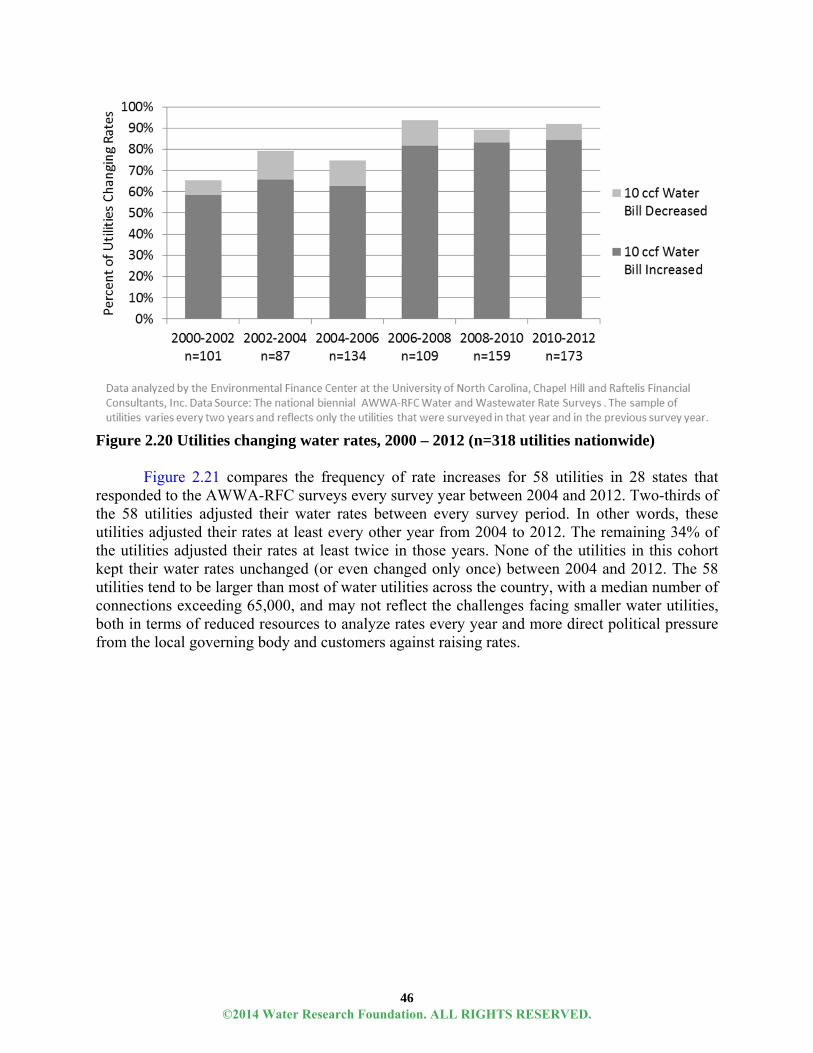
46
Figure 2.20 Utilities changing water rates, 2000 – 2012 (n=318 utilities nationwide)
Figure 2.21 compares the frequency of rate increases for 58 utilities in 28 states that
responded to the AWWA-RFC surveys every survey year between 2004 and 2012. Two-thirds of the 58 utilities adjusted their water rates between every survey period. In other words, these utilities adjusted their rates at least every other year from 2004 to 2012. The remaining 34% of the utilities adjusted their rates at least twice in those years. None of the utilities in this cohort kept their water rates unchanged (or even changed only once) between 2004 and 2012. The 58 utilities tend to be larger than most of water utilities across the country, with a median number of connections exceeding 65,000, and may not reflect the challenges facing smaller water utilities, both in terms of reduced resources to analyze rates every year and more direct political pressure from the local governing body and customers against raising rates.
©2014 Water Research Foundation. ALL RIGHTS RESERVED.

47
Figure 2.21 Frequency of water rate changes between biennial rates survey years between 2004 and 2012 for 58 utilities nationwide
In order to study the regional differences in rate increases, historic rates information
collected in statewide rates surveys from 3,102 utilities in GA, OH, NC, TX, and WI were compared. These surveys include a large number of smaller utilities and they show wide regional disparities in how frequently utilities raised rates since 2000. The percent of utilities changing rates from the previous year, by state, is shown in Figure 2.22. The percentages remain fairly consistent across the years within each state except in Ohio, even following the economic downturn. In fact, just as seen in the national trends, the incidence of rate changes slightly increased between 2008 and 2011 before dropping in 2012. On the other hand, the percentages varied widely among the states. In Georgia, North Carolina, and Texas, approximately 50% to 65% of utilities changed rates in any given year. Alternatively, in Wisconsin, fewer than 30% of utilities changed rates in any given year between 2000 and 2012, much lower than in all of the other states. This may be explained by the fact that in Wisconsin, unlike in the other five states, government-owned water utilities are financially regulated by the state’s Public Service Commission and must request state approval for rate increases in addition to the approval of their governing boards. This approval process in many cases requires additional resources and time that most likely influences the willingness to make frequent adjustments (see Section on Economic Regulation in Chapter 3).
©2014 Water Research Foundation. ALL RIGHTS RESERVED.

48
Figure 2.22 Percent of utilities changing rates in five states (n=3,102 utilities)
Figure 2.23 tracks how frequently a cohort of 1,966 utilities in the five states with rates
data collected for every year of the study changed rates in five consecutive years towards the end of the decade. The vast majority of utilities in all states raised rates at least once in the five year period, with most utilities adjusting rates approximately every other year. The distribution of rate adjustments varied significantly by state. For example, 42% of 393 North Carolina utilities changed rates nearly every year, but only 5% of 574 Wisconsin utilities did the same. In fact, 29% of Wisconsin’s utilities did not change rates at all between 2008 and 2012, far exceeding equivalent proportions in the four other states. Differing regulatory environments with respect to rate increases likely explain some of this variation. While local governments in Wisconsin are regulated by the Public Service Commission, local government in North Carolina and the other states are only regulated by their governing boards.
©2014 Water Research Foundation. ALL RIGHTS RESERVED.

49
Figure 2.23 Frequency of rate adjustments in 5 consecutive years among 1,966 utilities in five states
Similarly, Figure 2.24 shows the relationship between the frequency of annual rate
increases from 2006 to 2010 and credit rating. While the sample size of utilities varies (and is relatively small) with each credit rating and should be taken into account when assessing this figure, some trends can be discerned from the data. Of the utilities with credit ratings A1 and A2, for example, around 20% of these never changed their rates in the four year timespan. Utilities with higher credit ratings (although a relatively small group) had much larger percentages of utilities that increased rates occasionally or annually.
©2014 Water Research Foundation. ALL RIGHTS RESERVED.

50
Figure 2.24 Frequency of rate increases from 2006-2010 among 7 states Degree of Rate Changes
Rate changes are crucial for a utility’s financial health in order to keep revenues
consistent with rising costs, described in the “Trends in Utility Finance” section. And while there are a myriad of drivers behind rate increases, such as customer changes, cost increases, financial policy adjustments, the following analysis focuses on general trends. Analyses of historical rate adjustments in six states and in the nationwide AWWA-RFC rates dataset show great variation in trends across utilities between 2000 and 2012. In the following analyses, changes to the monthly-equivalent total (either water or water /wastewater for combined utilities) bill at one consumption point are computed between years to determine the rate change degree for each utility. Although utilities are frequently raising rates, the extent of the rate increases varies widely.
©2014 Water Research Foundation. ALL RIGHTS RESERVED.

51
Figure 2.25 shows the median and interquartile range (middle 50%) of biennial rate modifications of subsamples of 326 utilities in 50 states, District of Columbia, and 3 utilities in Canada as percent increases in the total monthly bill for 10 ccf between survey years from 2000 to 2012. The median rate changes fluctuated between 5% and 15% rate increases between rate surveys during this time, with the interquartile ranging between 0% and 23% between surveys. This indicates that while some utilities did not raise rates (or, in fact, lowered them), some utilities were able to secure more than 20% rate increases in two years’ time. The values of rate increases were highest between 2006 and 2012, during the economic recession, coinciding also with a period of increased frequency of rate increases among utilities nationwide. Interestingly, during those years, water utilities raised rates more frequently and at greater levels than in previous years possibly to compensate for recession-driven sale decreases.
Figure 2.25 Biennial nationwide rate modifications, 2000-2012 (n=329 utilities)
©2014 Water Research Foundation. ALL RIGHTS RESERVED.
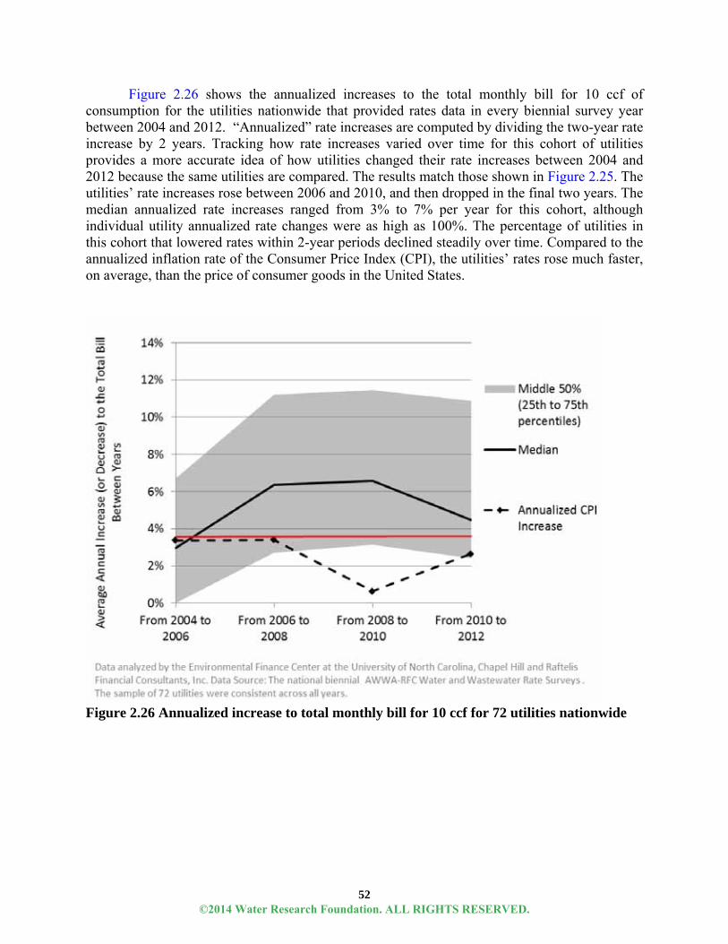
52
Figure 2.26 shows the annualized increases to the total monthly bill for 10 ccf of consumption for the utilities nationwide that provided rates data in every biennial survey year between 2004 and 2012. “Annualized” rate increases are computed by dividing the two-year rate increase by 2 years. Tracking how rate increases varied over time for this cohort of utilities provides a more accurate idea of how utilities changed their rate increases between 2004 and 2012 because the same utilities are compared. The results match those shown in Figure 2.25. The utilities’ rate increases rose between 2006 and 2010, and then dropped in the final two years. The median annualized rate increases ranged from 3% to 7% per year for this cohort, although individual utility annualized rate changes were as high as 100%. The percentage of utilities in this cohort that lowered rates within 2-year periods declined steadily over time. Compared to the annualized inflation rate of the Consumer Price Index (CPI), the utilities’ rates rose much faster, on average, than the price of consumer goods in the United States.
Figure 2.26 Annualized increase to total monthly bill for 10 ccf for 72 utilities nationwide
©2014 Water Research Foundation. ALL RIGHTS RESERVED.

53
Rate modifications varied geographically across the country. Figure 2.27 shows the median and interquartile ranges of percent changes in total monthly bills for utilities with rate modifications between consecutive years in five states: Georgia, North Carolina, Ohio, Texas, and Wisconsin. The median rate increase was 5% and 7% per year in North Carolina, Ohio, and Texas, while utilities in Georgia raised rates at much higher levels (medians between 10% and 15% per year) and utilities in Wisconsin that raised rates kept the increases low (medians below 5% per year).
While the median rate increase in each state remained relatively stable across the years – despite the economic recession and other changing conditions – the distribution of rate increases among utilities in each state was more varied as was the distributions between states. For example, the interquartile range of rate increases in North Carolina and Ohio were narrow and concentrated very close to the median, implying that utilities across those states were implementing rate increases that were relatively consistent with one another. In other states, such as in Wisconsin and Georgia, the interquartile range of rate increases was significantly larger, revealing a wider range of rate modifications statewide. In fact, data from Wisconsin show that while median increases for any particular year were low, a large portion of utilities that modified rates implemented very large rate increases, unlike in other states.
Similarly, in 2012, a quarter of the utilities that changed rates in Wisconsin raised rates by more than 30%. By comparison, the upper quartiles of rate increases in the other states usually began between 10% and 15%. The impact of Wisconsin’s financial regulation is evident when comparing the level of rate increases implemented by the local governments compared to those from the other states with no state oversight on local government rate increases.
©2014 Water Research Foundation. ALL RIGHTS RESERVED.
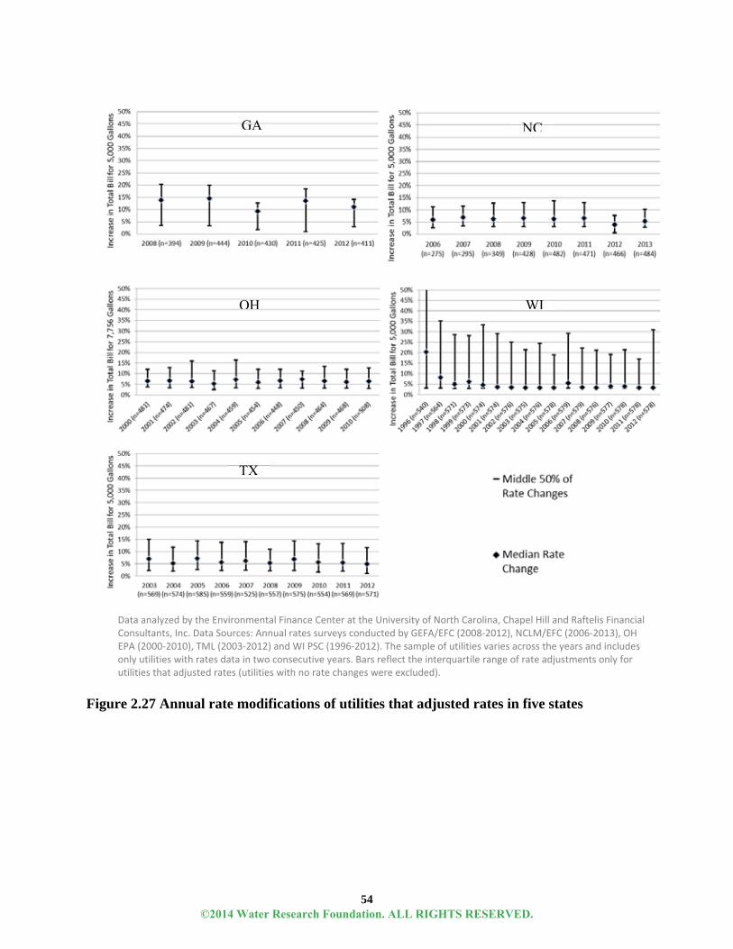
54
Figure 2.27 Annual rate modifications of utilities that adjusted rates in five states
GA NC
OH WI
TX
Data analyzed by the Environmental Finance Center at the University of North Carolina, Chapel Hill and Raftelis Financial Consultants, Inc. Data Sources: Annual rates surveys conducted by GEFA/EFC (2008‐2012), NCLM/EFC (2006‐2013), OH EPA (2000‐2010), TML (2003‐2012) and WI PSC (1996‐2012). The sample of utilities varies across the years and includes only utilities with rates data in two consecutive years. Bars reflect the interquartile range of rate adjustments only for utilities that adjusted rates (utilities with no rate changes were excluded).
©2014 Water Research Foundation. ALL RIGHTS RESERVED.

55
Utilities that increased rates less frequently tended to make larger rate increases than utilities that increase rates more often. This trend is illustrated in Figure 2.28 that compares average rate increases of utilities classified by their frequency of adjusting rates over a five-year period as determined in Figure 2.24. The average one-time rate adjustments are (sometimes drastically) higher for utilities that changed rates only once in five years compared to utilities that changed rates almost every year. In Ohio, for example, utilities that increased their rates only once in the five year period averaged a 19% rate increase, compared to an average annual increase of 7% for Ohio utilities that raised rates almost every year in the same time period. Figure 2.28 confirms the finding alluded to in Figure 2.27 regarding Wisconsin’s utilities tendency to either raise rates frequently at relatively low levels or raise rates infrequently at relatively high levels.
Figure 2.28 Average rate adjustment by frequency of raising rates among 1,966 utilities in five states
©2014 Water Research Foundation. ALL RIGHTS RESERVED.

56
Cumulative Rate Changes Although utilities that adjusted rates infrequently tended to have higher rate increases
than the annual increases of utilities that adjust rates annually, the cumulative effect of more frequent, smaller rate increases generally outsize the larger, one-time rate increases. Figure 2.29 shows the average cumulative rate increase over five years for utilities within each state based on how frequently they adjust rates. The utilities that increased rates more frequently had larger cumulative rate increases during a five-year period than those that raised rates only once in the five years in four states. For example, although the utilities in Georgia that raised rates almost every year only raised rates by an average of 9% per year, the cumulative rate increases amounted to an average of 44% after five years. By comparison, the Georgia utilities that raised rates only once in five years had a rate increase of 20%. Hence, there may be financial benefits for utilities to raise rates frequently: the annual rate increases can be small in size, avoiding customer rate shock, while enabling the utilities to accumulate greater rate increases over time than if the utility maintains the same rates for several years and requires a very large one-time rate increase.
Figure 2.29 Average 5-year cumulative rate increase by frequency of rate adjustments
These trends held true in every state except Wisconsin. This result is consistent with prior
observations that utilities in Wisconsin, more so than in the non-regulated states, that choose one-time rate increases tended to raise rates at much higher levels (more than five times on average) than the Wisconsin utilities that raises rates a lower-than-normal amount every year.
©2014 Water Research Foundation. ALL RIGHTS RESERVED.

57
The graphs discussed within this section indicate that, while there is some variability of rate increases between states, more frequent rate increases generally are associated with smaller rate increases at one time, but a larger cumulative increase over a five year time period.
Whether a utility increases rates annually or only once every five years, ultimately, rate increases should reflect utility cost increases, which can depend on inflation of costs of materials and equipment, rising debt, and other factors. These cumulative rate increases over time (whether they come frequently or infrequently) should be sufficient to increase revenues at a rate commensurate with utility costs. As previously discussed, more frequent, small rate adjustments are associated with larger cumulative rate increases than larger, infrequent rate adjustments.
Historical data on the share of utilities changing rates in a particular year, and the degree of utilities rate increases, reveals overall historic trends in cumulative rate increases. Figure 2.30 shows how the monthly water or monthly water and wastewater bill for a specific consumption point rose each year for the same cohort of 1,961 utilities in six states, along with cumulative Consumer Price Index inflation in the corresponding region for comparison. For example, by 2012, half of 194 utilities in Texas had a monthly total bill for 5,000 gallons that, in nominal terms, was at least 45% higher than in 2003. The middle half of these utilities had bills that were 27% - 67% higher in 2012 than in 2003. In those ten years, the Consumer Price Index for the South region rose by a total of 26%, indicating that more than three-quarters of the 194 Texas utilities raised water and/or combined between 2003-2012 faster than inflation and the rise of other consumer goods. Though the exact size of the cumulative rate increases varied from state to state, water/combined rates rose faster than inflation in all states. Prior to 2007, the median rate increase in Ohio and Texas was on par with inflation, and was in fact below inflation in Wisconsin. After 2007, CPI stagnated in all regions during the recession (resulting in deflation in one year), but water/combined rates continued to rise at a steady rate, resulting in more utilities raising rates faster than cumulative inflation in their region during that time period in all three states. In North Carolina, Georgia, and California, the majority of utilities raised rates faster than regional CPI inflation in recent years.
In many states, however, there were also utilities in the middle 50% whose rate increases failed to keep pace with inflation, particularly prior to 2007. It is possible that these utilities were in a financial position that did not require them to generate additional revenue, were experiencing a level of growth that covered increasing costs, or that they were unable or unwilling to make rate increases necessary to support a solid financial position on an ongoing basis. Ohio, Wisconsin, and Texas, for example, all saw a roughly 40% median cumulative increase over a ten-year timespan, but had a large percentage of utilities that did not increase rates at a pace higher than CPI inflation through 2007. North Carolina and Georgia had a much lower portion of utilities that did not raise rates commensurately with regional CPI inflation. There is significant variability of bill increases between the middle 50% of utilities for each state. This could reflect differences in utility governance at the city or county level or in local economies.
©2014 Water Research Foundation. ALL RIGHTS RESERVED.

58
Figure 2.30 Cumulative bill increases for 1,961 utilities in six states compared to CPI by region
©2014 Water Research Foundation. ALL RIGHTS RESERVED.

59
These regional trends match national trends observed from the AWWA-RFC rates survey data. Figure 2.31 shows the monthly bill for 10 ccf relative to the monthly bill in 2004 for a cohort of utilities nationwide. Much like trends in individual states, water charges increased at a rate faster than the national CPI after 2006. The median increase in nominal monthly bills from 2004 to 2012 was 50%, compared to a cumulative increase in CPI of 22% in the same time period.
Figure 2.31 Monthly charge for 10 ccf relative to 2004 charge for 72 nationwide utilities
Figure 2.32 shows the percent rate increase for 82 utilities nationwide by Moody’s most recent credit rating. Note that utility sample sizes for each credit rating vary (and are relatively low) and may have an impact on overall trends in rate increases. Utilities with slightly lower ratings (Aa2 and below) had smaller cumulative rate increases.
©2014 Water Research Foundation. ALL RIGHTS RESERVED.

60
Figure 2.32 Credit rating vs. percent rate increase from 2006 to 2010 for 82 utilities nationwide
Rate Increases at Different Consumption Levels
Rate structures usually comprise two or more elements with unique prices or rates, such as a
base charge and at least one volumetric rate (more if the utility uses a tiered rate structure). When adjusting rates, utilities can adjust some or all of these rate components, by the same or different percentage amounts. Based on how utilities adjust each element, the net financial effect of the rate adjustments on customers with different water use behavior can vary greatly. An obvious example is if a utility raises its non-residential rates but not its residential rates. Even rate adjustments for one customer class can affect those customers in different ways. For example, a utility might choose to raise the volumetric rates for higher levels of consumption for residential customers by 10% and avoid raising the base charge and lower block rates entirely. This would result in keeping the monthly charges unchanged for low water-using residential customers, such as one or two-person households, while raising them for high-water using residential customers, such as those who irrigate lawns during the summer. Sometimes, deciding on how to adjust different elements of the rate structure(s) is made deliberately to protect certain groups of customers from the brunt of the rate increases, or to send a price signal to specific customers to encourage water-using behavior that is consistent with utility objectives
Given the myriad of ways a utility can adjust its rate structure(s), customers’ bills change by a range of values. Although it is common (and easiest) to analyze and discuss utility rate increases in terms of a single percentage or dollar value (calculated as the change of the bill at one consumption point), bills at different consumption points are most likely changing by different amounts. In reality, the actual customer out-of-pocket expenditures are changing based on their changing water usage.
Figure 2.33 shows the median residential monthly water bill for four different consumption levels for a cohort of 58 utilities across the nation between 2004 and 2012. The four levels of consumption can be considered as different “service levels.” At 0 ccf, customers are paying for access.
©2014 Water Research Foundation. ALL RIGHTS RESERVED.
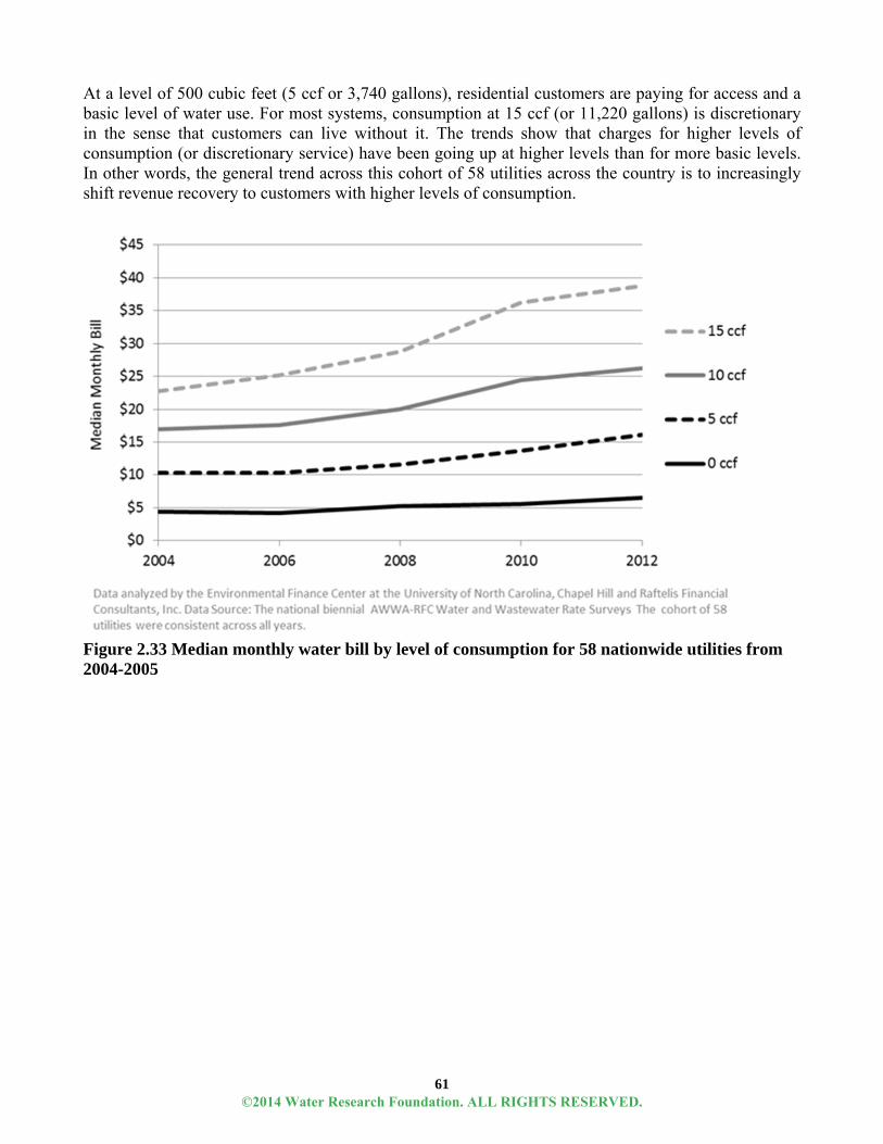
61
At a level of 500 cubic feet (5 ccf or 3,740 gallons), residential customers are paying for access and a basic level of water use. For most systems, consumption at 15 ccf (or 11,220 gallons) is discretionary in the sense that customers can live without it. The trends show that charges for higher levels of consumption (or discretionary service) have been going up at higher levels than for more basic levels. In other words, the general trend across this cohort of 58 utilities across the country is to increasingly shift revenue recovery to customers with higher levels of consumption.
Figure 2.33 Median monthly water bill by level of consumption for 58 nationwide utilities from 2004-2005
©2014 Water Research Foundation. ALL RIGHTS RESERVED.

62
Figure 2.34 shows similar trends at the state level at slightly different levels of consumption. When compared to one another, rate increases in Georgia at all levels of consumption are less than in North Carolina and Wisconsin. In North Carolina, service at all levels are more expensive than in the other two states and are becoming increasingly so at higher levels of service.
Figure 2.34 Median monthly water bill by level of consumption for 1,292water utilities in North Carolina, Georgia, and Wisconsin
Changes to Base Charges and Volumetric Rates
The analysis also looked at the changing balance between base charges and volumetric charges.
Utilities projecting a specific revenue goal in their budget may adjust the base charges and/or volumetric rates in various ways to reach their revenue goal. In allocating costs to the base charge or the volumetric rate, utilities balance many objectives.
Pricing structures that build cost recovery into the base charge provide a relatively stable stream of revenue, regardless of the season or other conditions that drive water demand. For example, in some coastal communities where the service population drops significantly during the off-season,
©2014 Water Research Foundation. ALL RIGHTS RESERVED.

63
base charges may be the primary source of revenue from the customers who leave town, and are necessary to continue to pay the utility’s fixed costs. Utilities with high fixed costs or a high degree of demand variability have an incentive to set high base charges in order to ensure sufficient revenue generation every month to pay for their fixed costs.
On the other hand, rate structures that put significant emphasis on base charges run into conflict with customer affordability and conservation goals. All customers pay the base charges, regardless of how little or how much water they use. The higher the utility sets its base charge, the more difficult it will be for low-income customers and the less financial impact a reduction in water use will have on a customer’s bill. Determining a balance between base and volumetric charges therefore represents a tradeoff between stable revenues and a fee structure that charges more to the customers with the most usage.
One way of examining the balance between base charges and volumetric rates is to compare base charges as a percent of the total bill at various levels of consumption. If a customer uses no water or wastewater service during a particular month, the base charge will represent 100% of their bill. The base charge will become a decreasing portion of a customer’s bill as consumption rises, but the exact ratio will depend upon the utility’s rate structure. Trends in this relationship can help illustrate revenue vulnerability trends across the industry.
An analysis of bills by their base charge percentages for 1,626 utilities in California, Georgia, North Carolina, and Wisconsin is shown in Figure 2.35. The graph shows the median portion of a customer’s bill at various levels of monthly consumption that is comprised of the base charge, by state. For example, among 443 Georgia utilities, half had designed their rate structures such that the monthly bill for 5,000 gallons is comprised at least 55% by the base charge and 45% by the volumetric charges. This means that a customer using less than 5,000 gallons/month at one of these utilities will contribute at least 55% of their bill towards fixed revenues for the utility. At higher consumption levels, the base charge comprises a decreasing portion of the monthly bill. The monthly bill at 10,000 gallons/month, for instance, was comprised of no more than 32% from the base charge for half of the 443 Georgia utilities.
The median lines in Figure 2.35 vary substantially across the four states, reflecting significant regional differences in rate structure objectives in the four regions. In general, utilities in the southeast (North Carolina and Georgia) tended to favor higher base charge portions in their rate structures compared to utilities in Wisconsin and California. In addition, the southeastern utilities more frequently included a consumption allowance with their base charges (as indicated by the flat median line in the left-hand corner of the graph). Wisconsin utilities relied the most heavily on variable revenues from their low consumption customers. By comparison, California utilities had the most variable rates at high consumption levels. More than half of the sampled California utilities had set up rate structures in which at least 90% of the bill for more than 10,000 gallons/month was comprised of volumetric rates. This could be the result of a strong, statewide initiative to encourage water conservation through pricing in the State of California (CUWCC 2012).
©2014 Water Research Foundation. ALL RIGHTS RESERVED.

64
Figure 2.35 Statewide median of base charges as percent of total bills by consumption level in four states
As with rate changes, the balance between base and volumetric charges changed over time. In
some cases, utilities conduct an extensive study to compare the breakdown of revenues and costs in terms of fixed versus variable, as was the case with the Charlotte-Mecklenburg Utilities Department (CMUD). By 2011, CMUD had one of the most variable water rate structures in the southeast. Residential customers inside the city limits were paying $2.40/month in water base charges plus $1.45/100 cubic feet for the first 400 cubic feet. This rate structure had base charge proportions that were in the bottom 10th percentile among 650 Georgia and North Carolina water rate structures in 2011, as shown in Figure 2.35. As a result of its highly-volumetric rate structure, CMUD was collecting up to 95% of its water and wastewater revenues from the volumetric rates and 5% from the base charges (CMUD 2012). Yet, the majority of the utility’s costs were fixed, going towards debt service, pay-go capital expenditures, and short-term fixed operations and maintenance costs (CMUD 2011).
As a consequence of the imbalance between fixed costs and fixed revenues, in July 2012, the utility raised the monthly water base charge to $4.65, lowered the first tier water rate to $0.98/100 cubic feet, and raised the second and third tier rates. By raising the base charge and lowering the first tier rate, CMUD effectively raised the base charge portion of its water rate structure significantly, and aligned closer to most water rate structures in Georgia and North Carolina, shown in Figure 2.36. At the beginning of the fiscal year, CMUD projected that this adjustment would result in increasing the proportion of revenues from base charges from 5% to 16% in 2012 (CMUD 2012).
©2014 Water Research Foundation. ALL RIGHTS RESERVED.
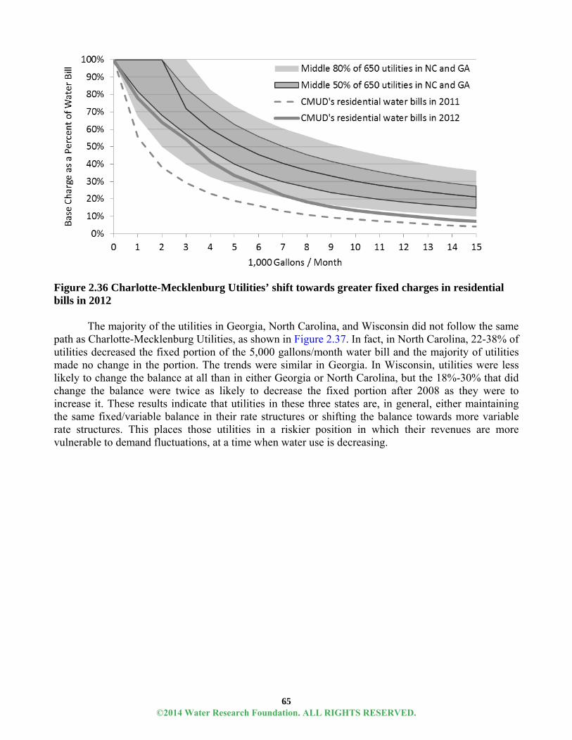
65
Figure 2.36 Charlotte-Mecklenburg Utilities’ shift towards greater fixed charges in residential bills in 2012
The majority of the utilities in Georgia, North Carolina, and Wisconsin did not follow the same path as Charlotte-Mecklenburg Utilities, as shown in Figure 2.37. In fact, in North Carolina, 22-38% of utilities decreased the fixed portion of the 5,000 gallons/month water bill and the majority of utilities made no change in the portion. The trends were similar in Georgia. In Wisconsin, utilities were less likely to change the balance at all than in either Georgia or North Carolina, but the 18%-30% that did change the balance were twice as likely to decrease the fixed portion after 2008 as they were to increase it. These results indicate that utilities in these three states are, in general, either maintaining the same fixed/variable balance in their rate structures or shifting the balance towards more variable rate structures. This places those utilities in a riskier position in which their revenues are more vulnerable to demand fluctuations, at a time when water use is decreasing.
©2014 Water Research Foundation. ALL RIGHTS RESERVED.

66
Figure 2.37 Annual changes to the base (fixed) charge portion of 5,000 gallons/month residential water bills in Georgia, North Carolina, and Wisconsin.
The extent to which the balance between fixed and variable charges changed after five years, from 2007 to 2012, for 1,260 utilities in the three states is shown in Figure 2.38. Each point represents one utility, and displays the base charge portion of the residential water monthly bill at 5,000 gallons in 2007 along the y-axis and in 2012 along the x-axis. The one-to-one line is displayed for orientation. Utilities that either did not adjust rates at all or adjusted the base charge and the volumetric rates by an equal percentage between 2007 and 2012 will be located along the one-to-one line: 37% of the 1,260 utilities fell on this line. The remaining 63% shifted the balance between base and volumetric rates in the five year period. Twice as many utilities decreased the base charge portion of their water bills than those that increased the portion (42% versus 21%, respectively). The extent of the adjustments varied widely. Many utilities changed the fixed portions by less than 20 percentage points. In some extremes, however, the change can be drastic. For example, one utility went from 70% fixed charge portion in 2007 to 7.4% in 2012, and another from 8% to 49%.
©2014 Water Research Foundation. ALL RIGHTS RESERVED.

67
Figure 2.38 Base (fixed) charge portion of the residential water bill for 5,000 gallons/month in 2007 and 2012 for 1,260 utilities in Georgia, North Carolina, and Wisconsin.
The relationship between fixed and variable charges can be delicate, and can often impact more than just a utility’s revenues. Figure 2.39, for example, shows variation in the fixed portion of water and combined utility bills for 5,000 gallons by credit rating for 38 utilities nationwide. Median fixed bill portions consistently increased as credit ratings worsened. Sample sizes between utilities, however, varied significantly and may have an impact on the trends seen in this figure.
©2014 Water Research Foundation. ALL RIGHTS RESERVED.

68
Figure 2.39 Fixed portion of 5,000 gallon bill in 2011 by most recent credit rating for 38 water and combined utilities nationwide.
Utilities that increase reliance on volumetric charges also increase revenue vulnerability due to
normal cyclic weather induced changes in use. Furthermore, raising the volumetric rates faster than the base charges may provide a price signal and a financial incentive for customers to curtail their demands since their water bills are more sensitive to their water use levels. Reducing demands will reduce the revenues for the utilities, which are more dependent on demand now that the base charge portions of the bills have been effectively lowered.
Relationship between Rate Structures, Rate Increases, and Revenues
As shown in the sections above, the complexity of rate structures provides utilities with many
adjustment options, including the type of volumetric rate structure. The most common volume-based rate structures for water and wastewater utilities are uniform rate structures (in which the marginal price for each additional unit of water consumed remains constant) and blocked rate structures (in which the marginal price either increases or decreases as consumption increases).
The impacts of these rate structure types on utility revenues vary significantly. Compared to uniform rate structures, increasing block rate structures inflate the revenues generated from higher consumption levels. Thus, the “premium” customers who use large volumes of water pay a higher share of the utility’s total revenues under an increasing block rate structure than the “basic” customers. Yet, high water use is more likely to include discretionary uses of water that are more vulnerable to fluctuations than baseline, indoor uses of water. Setting high marginal prices for high volumes of water simultaneously increases the proportion of revenue expected to be generated from that demand while at the same time sending a price signal that might cause customers to curtail those discretionary water uses. Consequently, increasing the rate differential between blocks puts more of a utility’s revenue at risk in the face of declining demand (particularly at the higher tiers which are more sensitive to price increases) while simultaneously incentivizing customers to reduce those high demands.
©2014 Water Research Foundation. ALL RIGHTS RESERVED.

69
In addition to different rate structures incentivizing different customer water use behavior and influencing the utilities’ revenues, rate increases alone impact water use. Water and wastewater price elasticity has been studied extensively by researchers for decades. Two meta-analyses on residential price elasticity found that the average estimated price elasticity for water (and wastewater) in over 300 research studies was between -0.41 and -0.51, and generally ranged between 0 and -0.75 (Dalhuisen et al. 2003; Espey et al. 1997). The authors of the two meta-analyses noted that in most of the research studies they reviewed, price elasticity was estimated to be statistically significant. In other words, extensive research has determined that residential customers, on average, respond to rate increases by lowering their consumption to some degree. The extent to which customers decrease their consumption for a given rate increase, however, is not clear from all of the studies, and varies depending on several factors including location, season, rate structure, income, weather, water use, and other factors (Dalhuisen et al. 2003; Espey et al.1997).
At the utility level, this creates an important relationship between rate increases and revenues. What the studies agree on is that if a utility raises rates by, say, 10%, and nothing else changes for the next year (including weather, number of customers, income levels, policies, household appliances, etc.), the utility would most likely see their revenues increase by less than 10%. In reality, all of the other factors that affect water use and revenues will never be identical from one year to the next, and thus revenues may increase or decrease by more than 10% for some utilities, but not likely in sole response to price.
On a national level, more utilities (57%) had greater cumulative rate increases on their 10 ccf (7,480 gallons) monthly water and/or wastewater bill than the resulting percentage increase in their total operating revenues, as reported in the 2004 and 2012 AWWA-RFC Water and Wastewater Rates Surveys and shown in Figure 2.40. In fact, three utilities had lower revenues in 2012 than in 2004, despite raising their residential rates. The relationship between rate and operating revenue increases may also be dependent on the extent by which rates are raised.
For high rate increases (marks on the upper right side of the graph), increases in operating revenues were much more likely to be lower than the increases in the rates. All but one of the 19 utilities that doubled their rates between 2004 and 2012 had operating revenue increases that were substantially lower than the rate increase. At the other end of the spectrum, utilities that only raised rates $10 per month or less and by 40% or less had greater revenue increases than rate increases. As explained above, these may be because of increases to demands due to other non-price related factors. In fact, more than half of these utilities had greater average daily sales (total demand) in 2012 relative to 2004, compared to only 20% of the utilities that more than doubled their rates and by at least $20/month. Further, as explained above, it is perhaps because of the declining sales and lower revenue increases that those utilities applied such high rate increases, to generate sufficient revenues in future years.
©2014 Water Research Foundation. ALL RIGHTS RESERVED.

70
Figure 2.40 Increases in rates and operating revenues for 94 utilities nationwide, 2004 to 2012
Similar relationships between rate and revenue increases were evident among 566 utilities in
Ohio, North Carolina, and Texas, as shown in Figure 2.41. Generally, utilities had a diverse range of rate and revenue changes over the three or four year period. In all three states, 61%-66% of the utilities had lower revenue increases than rate increases (points below the 1:1 line), and almost every utility that raised rates by more than 50% had relatively lower revenue increases. A handful of utilities were even in the unfortunate position of having decreasing revenues despite increasing rates. On the other hand, the utilities that had relatively small rate increases were more likely to have revenue increases commensurate with or greater than the rate increase.
©2014 Water Research Foundation. ALL RIGHTS RESERVED.

71
Figure 2.41 Increases in rates and revenues among 566 utilities in three states.
These analyses suggest three important lessons for utilities. 1) Revenues usually increase when rates increase, despite a downward pressure on customer demand due to elasticity. In Figures 2.40 and 2.41, revenue and rate increases are positively correlated. 2) Generally, larger rate increases is associated with disproportionately lower revenue increases. This is most likely a result of underlying factors, as opposed to the rate increases – a topic worth further exploration. 3) The relationship between rate and revenue increases is complicated and differs from utility to utility. Two utilities with identical rate increases may have very different outcomes on revenue increases, even in the same state or region. There is no single rule-of-thumb equation that utilities can use to accurately predict the effect of a rate increase on revenues, given that many other factors beyond the control of the utility, will affect revenues. Furthermore, the relationship between rate increases and revenue increases works
DataanalyzedbytheEnvironmentalFinanceCenterattheUniversityofNorthCarolina,ChapelHillandRaftelisFinancialConsultants,Inc.Lineindicatesthe1‐to‐1ratiobelow
©2014 Water Research Foundation. ALL RIGHTS RESERVED.

72
in both directions: rate increases may drive down demand which will lower revenue increases, and lower revenue increases may necessitate higher rate increases. Utilities will probably find it difficult to raise their way out of a significant revenue shortfall; since higher rate increases tend to yield disproportionately lower revenue increases. Additional strategies, many of which are described in this report, should be considered in addition to raising rates when a utility experiences large revenue gaps.
Relationship of Rate Increases and Utility Financial Performance
As shown in Figures 2.27 and 2.28, utilities that raise rates more frequently usually do so with
smaller annual rate increases that ultimately result in larger cumulative rate increases than utilities with infrequent rate increases. A higher cumulative rate increase, however, is not the goal of a well-run water utility. The ultimate financial goal of a utility is strong financial performance and self-sufficiency. Do utilities that raise rates more frequently using smaller annual increases fare better financially than utilities that raise rates infrequently with larger one-time rate increases? It was explained in the previous discussion; for instance, that utilities with larger rate increases may have disproportionately lower revenue increases. Does this put utilities with large one-time rate increases or the utilities with larger cumulative rate increases over time at a disadvantage financially?
Figure 2.42 displays the range of non-capital operating ratios (operating revenues divided by operating expenses less depreciation) for a cohort of 531 utilities in three states, categorized by whether the utility did not change rates in four years, occasionally changed rates, or changed rates almost every year (3 or 4 times in four years). The non-capital operating ratios for the four years were averaged to produce a mean non-capital operating ratio for each utility. The graph displays the middle 50% of the average ratios in each frequency category in each state.
The results are inconclusive. There are no clear indications that utilities that raised rates more or less frequently fared any better than the others using this financial metric. In Texas, for example, the interquartile range is narrower on the high end for utilities that raised rates almost every year versus utilities that only occasionally raised rates, implying that utilities that raised rates more frequently were more likely to have higher ratios than the others. On the other hand, in North Carolina, the reverse proved true. The utilities that did not raise rates at all in four years (a sample of 10 utilities) out-performed the utilities that raised rates. It may be that these ten utilities did not raise rates because their revenues were already sufficient to cover their expenditures.
©2014 Water Research Foundation. ALL RIGHTS RESERVED.

73
Figure 2.42 Range of four-year average non-capital operating ratios by utilities’ frequency of adjusting rates for 531 utilities in three states
If financial ratios drive rate increases for many utilities, a correlation would be expected
between one year’s financial ratio and the next year’s rate increase. Figure 2.43 displays this relationship for the same cohort of 531 utilities in North Carolina, Ohio, and Texas. It is interesting to note that some of the largest rate increases occurred for utilities that had a non-capital operating ratio at or near the 1.0 threshold. In North Carolina, a large cluster of utilities that had ratios below 1.0 (higher O&M expenditures than operating revenues) attempted to rectify their financial condition by raising rates significantly the next year. In Texas and North Carolina, utilities that had some of the highest ratios, implying a surplus of revenues, had lower rate increases than the rest of the utilities, as expected. Yet, in Ohio, a significant portion of utilities with high ratios still raised rates by more than 10% in the subsequent year. While it appears that financial performance may be partially driving rate increases in these three states, it is not the only factor that utilities are considering when they decide on rate increases. There may be other financial performance indicators, such as debt service coverage ratio targets, that influence the decision. Furthermore, the financial outlook might be more influential on rate setting than a retrospective analysis of past and current financial performance, particularly when capital projects are planned to be implemented soon.
©2014 Water Research Foundation. ALL RIGHTS RESERVED.

74
Figure 2.43 Rate increases one year after the reported non-capital operating ratio for 531 utilities in three states, over three years
DataanalyzedbytheEnvironmentalFinanceCenterattheUniversityofNorthCarolina,ChapelHillandRaftelisFinancialConsultants,Inc.Thecohortofutilitiesremainedthesameforallthreeyearsineachstate.
©2014 Water Research Foundation. ALL RIGHTS RESERVED.
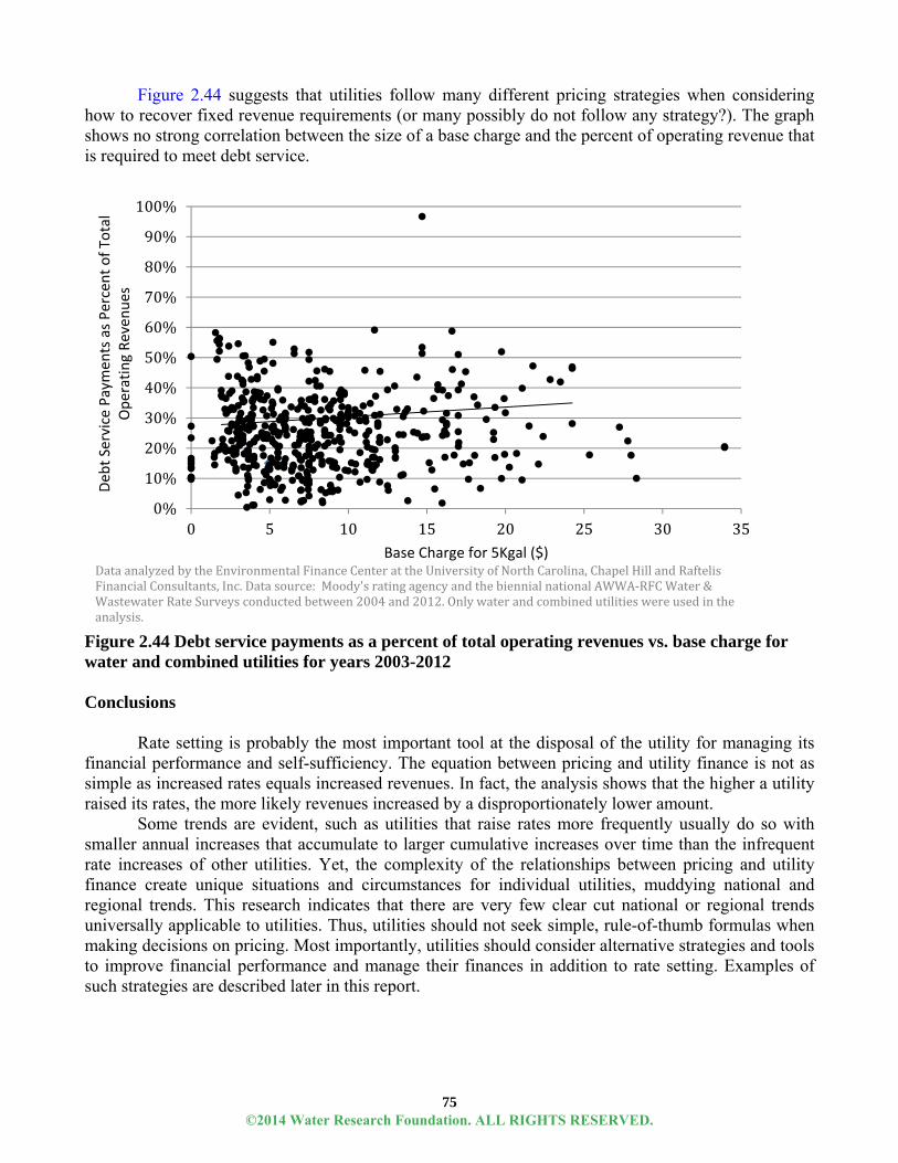
75
Figure 2.44 suggests that utilities follow many different pricing strategies when considering how to recover fixed revenue requirements (or many possibly do not follow any strategy?). The graph shows no strong correlation between the size of a base charge and the percent of operating revenue that is required to meet debt service.
Figure 2.44 Debt service payments as a percent of total operating revenues vs. base charge for water and combined utilities for years 2003-2012
Conclusions
Rate setting is probably the most important tool at the disposal of the utility for managing its financial performance and self-sufficiency. The equation between pricing and utility finance is not as simple as increased rates equals increased revenues. In fact, the analysis shows that the higher a utility raised its rates, the more likely revenues increased by a disproportionately lower amount.
Some trends are evident, such as utilities that raise rates more frequently usually do so with smaller annual increases that accumulate to larger cumulative increases over time than the infrequent rate increases of other utilities. Yet, the complexity of the relationships between pricing and utility finance create unique situations and circumstances for individual utilities, muddying national and regional trends. This research indicates that there are very few clear cut national or regional trends universally applicable to utilities. Thus, utilities should not seek simple, rule-of-thumb formulas when making decisions on pricing. Most importantly, utilities should consider alternative strategies and tools to improve financial performance and manage their finances in addition to rate setting. Examples of such strategies are described later in this report.
0%
10%
20%
30%
40%
50%
60%
70%
80%
90%
100%
0 5 10 15 20 25 30 35
Deb
t Service Paymen
ts as Percent of To
tal
Operating Reven
ues
Base Charge for 5Kgal ($)Dataanalyzed bytheEnvironmentalFinanceCenterattheUniversityofNorthCarolina,ChapelHillandRaftelisFinancialConsultants,Inc.Datasource:Moody'sratingagencyandthebiennialnationalAWWA‐RFCWater&WastewaterRateSurveysconductedbetween2004and2012.Onlywaterandcombinedutilitieswereusedintheanalysis.
©2014 Water Research Foundation. ALL RIGHTS RESERVED.

76
References
(AWWA) American Water Works Association. 2012. M1: Principle of Water Rates, Fees and Charges, 6th ed. Denver: Colo.: AWWA.
(CUWCC) California Urban Water Conservation Council. 2012. Utility Operations: Programs Resource Center. Sacramento, Calif.: CUWCC. [Online]. Available: <http://www.cuwcc.org/mou/bmp1-utility-operations-programs.aspx> [cited July 30, 2012]
(CMUD) Charlotte-Mecklenburg Utilities Department. 2011. Financial Planning Workshop Fall 2011 Presentation. Provided directly to the authors on May 8, 2012. Charlotte, N.C.: Charlotte-Mecklenburg Utilities Department.
(CMUD) Charlotte-Mecklenburg Utilities Department. 2012. Primary data provided directly to the authors on October 25, 2012. Charlotte, N.C.: Charlotte-Mecklenburg Utilities Department.
Dalhusien, J.M., Florax, R.J.G., de Groot, H.L.F., Nijkamp, P. 2003. Price and Income Elasticities of Residential Water Demand: A Meta-Analysis. Land Economics, 79(2): 292-308.
Espey, M., Espey, J. Shaw, W.D. 1997. Price Elasticity of Residential Demand for Water: A Meta-Analysis. Water Resources Research, 33(6): 1369-1374.
Fitch Ratings. 2011. U.S. Water and Sewer Revenue Bond Rating Criteria. New York, N.Y.: Fitch Ratings.
(USEPA) U.S. Environmental Protection Agency. 2011. Safe Drinking Water Information System Database [Online]. Available: EPA.gov. <http://www.epa.gov/enviro/facts/sdwis/search.html> [cited January 2011]
©2014 Water Research Foundation. ALL RIGHTS RESERVED.

77
CHAPTER 3:
FACTORS INFLUENCING REVENUE RESILIENCY SERVICE AREA SIZE AND DIVERSITY Introduction
Perhaps one of the most generalizable determinants of utility financial performance is facility size and customer base. Larger utilities can take advantage of economies of scale and spread their costs (which are mostly fixed) over a greater number of customers, thereby reducing costs per account. Smaller utilities have many of the same fixed costs and requirements with fewer customers to cover costs. Additionally, utility staff may lack time and expertise to strategically finance their utility. Larger systems are also more likely to have a diverse customer base (i.e. a healthy mix of residential, commercial, industrial, and wholesale customers) and are less vulnerable to revenue fluctuations as a result of individual customer behavior change. The following chapter explores utility financial trends in the context of service size area and diversity.
Key Points
Utilities serving a larger customer base tend to have lower rates and stronger financial performance metrics than their smaller counterparts.
Water utilities have very different customer type diversity profiles with some utilities almost exclusively relying on residential customers and others with a broader non-residential and residential mix.
Utilities with a larger percentage of industrial or wholesales tend to have stronger financial metrics. On the other hand, utilities reporting a reliance on a small number of very large customers are more at risk of sudden revenue drops due to the loss of one or two customers.
System Size
Figure 3.1 reiterates the notion that larger utilities are generally more financially secure than smaller utilities; it shows larger utilities tend to have higher operating ratios. In the 2012 AWWA-RFC Water and Wastewater Rates Survey, none of the utilities serving more than 150,000 accounts reported having operating ratios less than 1.0 (an indication that operating revenues fell short of operating expenses), a fate that several smaller systems did report.
©2014 Water Research Foundation. ALL RIGHTS RESERVED.

78
Figure 3.1 Operating ratio and number of accounts for 286 utilities nationwide in 2012
The AWWA-RFC survey sample has a disproportionate number of large systems in its sample.
An analysis of statewide data provides additional insight into the financial challenges of smaller systems. In North Carolina, 34% of local government utilities serving fewer than 1,000 connections had greater debt service and operations and maintenance expenses than the total operating revenues they collected from customer charges in FY2012, as shown in Table 3.1. In fact, 17% did not collect sufficient revenue in that fiscal year to pay for their day-to-day expenses alone. By comparison, only 8% of utilities serving more than 10,000 connections had debt service and operation and maintenance expenses that exceeded operating revenues. These financial stressors carry over to rate setting such that even though they are more likely to be suffering losses, smaller systems are also more likely to have higher rates than larger utilities as shown in Table 3.2.
Table 3.1
Utility financial performance in FY2012 among 382 local government utilities in North Carolina, by utility size
Number of service connections
Number of utilities
Operating revenues
insufficient to cover operations and maintenance
expenses
Operating revenues insufficient to cover
operations and maintenance
expenses plus debt service
Operating revenues sufficient to cover debt service and operations and maintenance
expenses 1-999 162 17% 17% 66% 1,000 – 9,999 172 5% 21% 74% 10,000+ 48 0% 8% 92% Source: Adapted from (Eskaf et al. 2013)
©2014 Water Research Foundation. ALL RIGHTS RESERVED.
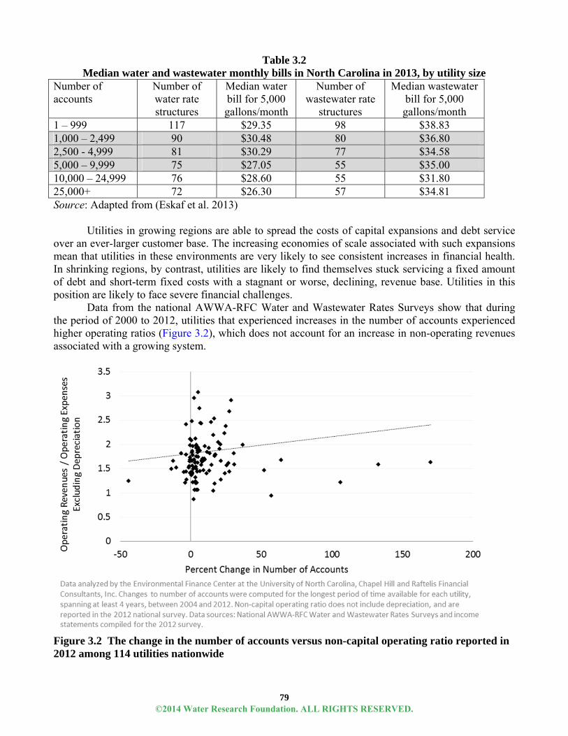
79
Table 3.2 Median water and wastewater monthly bills in North Carolina in 2013, by utility size
Number of accounts
Number of water rate structures
Median water bill for 5,000 gallons/month
Number of wastewater rate
structures
Median wastewater bill for 5,000 gallons/month
1 – 999 117 $29.35 98 $38.83 1,000 – 2,499 90 $30.48 80 $36.80 2,500 - 4,999 81 $30.29 77 $34.58 5,000 – 9,999 75 $27.05 55 $35.00 10,000 – 24,999 76 $28.60 55 $31.80 25,000+ 72 $26.30 57 $34.81 Source: Adapted from (Eskaf et al. 2013)
Utilities in growing regions are able to spread the costs of capital expansions and debt service
over an ever-larger customer base. The increasing economies of scale associated with such expansions mean that utilities in these environments are very likely to see consistent increases in financial health. In shrinking regions, by contrast, utilities are likely to find themselves stuck servicing a fixed amount of debt and short-term fixed costs with a stagnant or worse, declining, revenue base. Utilities in this position are likely to face severe financial challenges.
Data from the national AWWA-RFC Water and Wastewater Rates Surveys show that during the period of 2000 to 2012, utilities that experienced increases in the number of accounts experienced higher operating ratios (Figure 3.2), which does not account for an increase in non-operating revenues associated with a growing system.
Figure 3.2 The change in the number of accounts versus non-capital operating ratio reported in 2012 among 114 utilities nationwide
©2014 Water Research Foundation. ALL RIGHTS RESERVED.

80
Diversity of Customer Base
The concept of customer or market diversity comes up in any discussion of financial resiliency; the utility sector is no exception. Most utilities provide different types of services (water, irrigation water, wastewater, supplemental services) to several types of customers: single-family residential, multi-family residential, commercial, industrial, institutional, and other utilities (wholesale service). The relative share of a utility’s sales consumed by different customer sectors can affect the utility’s revenue and costs, and the vulnerability of its revenue generation to customer demand fluctuations.
An analysis of data in North Carolina illustrates potential revenue vulnerability for utilities that generate a significant amount of revenue from a small number of (usually non-residential) customers are more susceptible to revenue loss than utilities that spread their revenue generation across a greater number of customers. During 2010, 5% of 255 North Carolina utilities reportedly generated more than half of their total annual revenues from their five single largest customers (Figure 3.3, adapted from Eskaf, Hughes, and Nida 2011). If any one of these five customers left town, the utility would generate much less revenue in the subsequent year without a corresponding decrease in costs since the majority of expenses are fixed at least in the short-term.
Source: (Eskaf, Hughes, and Nida 2011) Figure 3.3 Breakdown of 255 North Carolina utilities based on the percentage of the utility’s total annual revenues generated by the 5 largest customers
Utilities that operate as wholesale-only (as opposed to retail) utilities often are under the same pressure as utilities with a large dependence on a few industrial customers. Wholesale utilities, such as the Metropolitan Water District of Southern California, sell water exclusively to surrounding utilities and do not provide direct water service to residential or commercial customers. Their revenue stream is sensitive to fluctuations in purchases from other utilities. Because their purchasing utilities may implement policies that affect demand (by implementing conservation-oriented rates, for example), wholesale utilities may have less control than retail utilities over their water demands, sales, and financial condition, although they have the option to address this issue in contracts.
©2014 Water Research Foundation. ALL RIGHTS RESERVED.

81
Local Water Supply Plan (LWSP) data from North Carolina Department of Environment and Natural Resources and financial performance data from the North Carolina Local Government Commission shows the variation in the importance of industrial sales across the state. A utility whose revenue largely comes from one or two large customers are subject to similar revenue vulnerability as wholesale utilities. However, despite the potential for more severe revenue fluctuation due to the loss of large customers, many utilities with a more diverse customer base that includes large industrial users have historically performed relatively well in North Carolina. While the trend is fairly weak, Figures 3.4 and 3.5 show that water utilities that sold a greater percentage of their output to industrial customers and to other utilities, respectively, tended to have higher operating ratios than those with lower sales to those types of customers. This trend may be due as much to the challenges facing utilities that focus on residential customers as it is to the inherent stability of depending on industrial customers.
Figure 3.4 Operating ratios of 363 North Carolina utilities by share of water sales to industrial customers
©2014 Water Research Foundation. ALL RIGHTS RESERVED.

82
Figure 3.5 Operating ratios of 363 North Carolina utilities by share of water sales to other utilities References Eskaf, S., D. Tucker, D. Batten, A. Patel and C. Nida. 2013. Water and Wastewater Rates and Rate
Structures in North Carolina, January 2013. Chapel Hill, N.C.: NC League of Municipalities and the Environmental Finance Center at the University of North Carolina. [Online]. Available: <http://efc.unc.edu/projects/NCWaterRates.htm> [cited May 31, 2013]
Eskaf, S., J. Hughes and C. Nida. 2011. Results of the 2010 North Carolina Water and Wastewater Financial Practices and Policies Survey. Chapel Hill, N.C.: NC League of Municipalities and the Environmental Finance Center at the University of North Carolina. [Online]. Available: <http://www.efc.unc.edu/publications> [cited May 31, 2013].
WATER USE AND WEATHER Introduction
Under the prevalent pricing models of water utilities across the United States and Canada, customer water use patterns have a very strong influence on utilities’ revenues and, by extension, on utility financial performance. Conversely, many utilities have incorporated pricing into their tools for impacting use. Understanding and managing this price-usage nexus is critical for utility managers that navigate between conservation goals and revenue requirements. As explained in the Trends in Utility Finance section, commodity charges generate revenue directly from the volume of water sold and are often the main source of revenue for water and wastewater utilities. When sales fall, revenues typically fall with them. But a decrease in water sales, however, does not lead to a commensurate reduction in utility expenses (further explained in the Trends in Utility Finance section). Without constant attention to pricing levels and structures, consistent decreases in water use from year to year can lead to significant revenue shortfalls for utilities. While many utilities have an expressed goal of reducing water usage, excessive declines in water use over recent years have caught many utilities off-guard, as
©2014 Water Research Foundation. ALL RIGHTS RESERVED.

83
revenues have fallen below predicted levels. As significant a significant driver of water use, weather can compound the relationship and its predictability, particularly in a time of climate extremities
Key Points
Water use for many utilities is the defining characteristic in the revenue consistency (and sometimes health) under current pricing and finance models.
National trends indicate that average water use per capita and per account is generally decreasing over time.
These trends corresponded with increasing drought trends across the country. Droughts in the United States were more significant in 2002-2004, 2006-2007, and from 2011 onwards, when at least 10% of land was in extreme or exceptional drought.
Such high drought prevalence is indicative of the need for utilities to develop revenue response strategies in conjunction with water shortage response strategies to help maintain utility financial health in times of restrictions.
Detailed analysis of large datasets of utilities within two states in separate regions of the country (NC and TX), show variation across utilities and regions that reinforces the danger of relying on generalized assumptions.
o In North Carolina, long-term trends of declining average residential use are more apparent than short-term fluctuations. Within North Carolina, utilities experienced extreme fluctuations in sales trends suggesting differences underlying factors from the implementation of water efficiency to customer migration.
o Although average residential water use declined for slightly more utilities than not, the Texas municipalities in this analysis were almost evenly split between those that reported increasing average residential water use and those that reported it decreasing.
These trends have a direct impact on the water pricing, and vice versa. Understanding the pricing-usage nexus should be a leading component of revenue projection.
National Trends
Literature on water use trends shows a convincing trend of increasing water use efficiency across the country. A look at four end use studies since 1995 shows that indoor residential water use was observed to be between 13.3% and 42.7% lower for a family living in a highly efficient new home (DeOreo and Mayer 2012). In another study, when controlling for weather and other variables, households in 2008 used nearly 12,000 gallons less annually than an identical household in 1978 (Rockaway et al. 2011). The overwhelming evidence, from research presented both here and elsewhere, supports a general trend of decreasing water consumption over the last decade, although regional differences may exist.
The national AWWA-RFC Water and Wastewater Rates Surveys, conducted biennially from 2000 to 2012, collected data on daily water sales in million gallons per day (MGD) and the number of water accounts for hundreds of utilities across the United States. Daily water sales included the aggregated utility-wide water sales to all customer types, including residential, commercial, industrial, institutional, and wholesale. Of the utilities that responded, 69 utilities in 32 states provided data on daily water sales and the number of water accounts in every survey from 2004 through 2012.
Figure 3.6 displays the median daily water sales and median number of water accounts in this cohort of 69 utilities between 2004 and 2012. While the number of water accounts increased over time due to population and customer base growth, the utility-wide median daily water sales decreased steadily over time (an 8.7% reduction from 2004 to 2012). This means that although the number of
©2014 Water Research Foundation. ALL RIGHTS RESERVED.

84
customers increased, the total water demand decreased over time for at least half of the 69 utilities. In fact, 47 out of the 69 (68%) utilities had lower daily water sales in 2012 compared to 2004, even though 60 out of the 69 (87%) utilities gained water customers during that time period. Declining total sales translates directly to lower revenues for utilities. To compensate, utilities would have had to raise rates in order to avoid declining revenues.
Figure 3.6 Daily water sales and number of water accounts among 69 utilities nationwide from 2004 to 2012.
The overall trends shown in Figure 3.6 were not seen for every individual utility studied. Figure 3.7 shows very different trends among utilities in the dataset. The degree to which daily water sales changed over time is shown in Figure 3.7, which compares daily water sales in 2012 to water sales in 2000 and 2006, in order to check in on the consistency of the trend. The analysis shows that despite a widespread increase in the number of water accounts, the majority of utilities had lower total daily water sales in 2012 than both comparison years. Using the years 2000 to 2006 as a baseline, 63% and 60% of the surveyed utilities, respectively, saw a reduction in total water sales when compared to 2012. In almost any industry, lowering sales of a product by more than 25% can be devastating to revenues, and such is the case for the water utilities as well. Although there are a number of factors explored later in this report that could have been driving this change in one particular year (2012), the point is that, despite why, sales declined for the majority of utilities.
©2014 Water Research Foundation. ALL RIGHTS RESERVED.

85
Figure 3.7 Differences in water sold and number of accounts in 2012 compared to the past decade Regional Trends
These national trends indicate that average water use per account is generally decreasing over time. At the regional level, however, results varied, implying that there may be regional trends that contradict the overall, national trends. In this analysis, the average residential water use data for larger samples of utilities in North Carolina and in Texas – two geographically disparate states with different climates – are compared. Data on water use in North Carolina were obtained from the North Carolina Division of Water Resources’ Local Water Supply Plans, which are plans in the form of questionnaires that all local government and large community water systems are required to complete. The LWSPs were completed in 1997, 2002, 2007, and updated once a year since then. The questionnaires asked water systems to report their average daily “use” (sales) in MGD and the number of metered connections, by customer class. From these data, the average household water use was calculated for this analysis in gallons/month. For Texas, hundreds of municipal water utilities directly reported their average residential water use, in gallons/month, to the Texas Municipal League as part of their annual Water and Wastewater Rates Surveys. For both states, analyses are presented on the changing average household (residential) water use in gallons/month, and not at the aggregated, utility-wide total sales in MGD.
In North Carolina, average residential water use has been declining steadily in the past decade. Figure 3.8 tracks the median and interquartile range of average residential water use among a cohort of 217 water systems in North Carolina for which data were available in every year. The median decreased from 5,083 gallons/month in 1997 to 4,292 gallons/month in 2010. On the low end, 38% of these systems’ average residential use was lower than 4,000 gallons/month in 2010, up from 19% in 1997.
©2014 Water Research Foundation. ALL RIGHTS RESERVED.
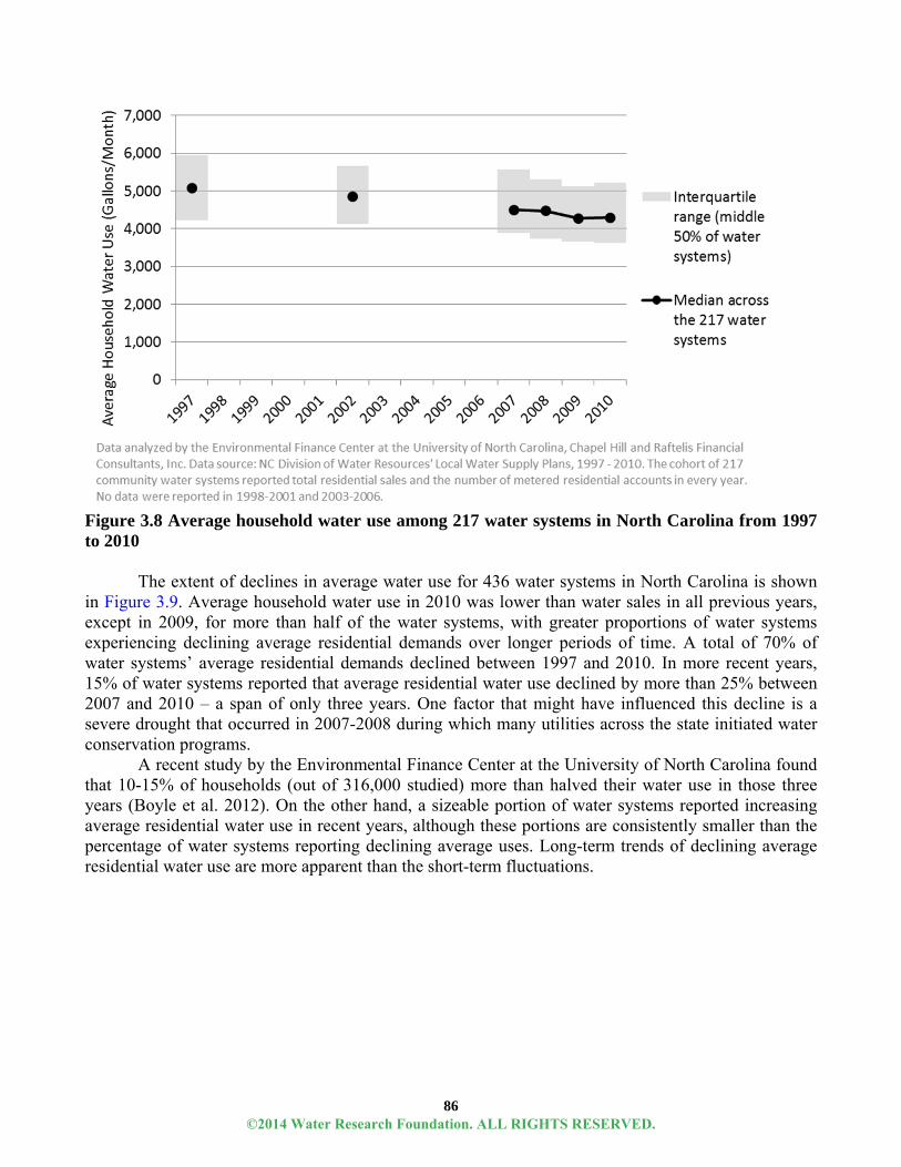
86
Figure 3.8 Average household water use among 217 water systems in North Carolina from 1997 to 2010
The extent of declines in average water use for 436 water systems in North Carolina is shown in Figure 3.9. Average household water use in 2010 was lower than water sales in all previous years, except in 2009, for more than half of the water systems, with greater proportions of water systems experiencing declining average residential demands over longer periods of time. A total of 70% of water systems’ average residential demands declined between 1997 and 2010. In more recent years, 15% of water systems reported that average residential water use declined by more than 25% between 2007 and 2010 – a span of only three years. One factor that might have influenced this decline is a severe drought that occurred in 2007-2008 during which many utilities across the state initiated water conservation programs.
A recent study by the Environmental Finance Center at the University of North Carolina found that 10-15% of households (out of 316,000 studied) more than halved their water use in those three years (Boyle et al. 2012). On the other hand, a sizeable portion of water systems reported increasing average residential water use in recent years, although these portions are consistently smaller than the percentage of water systems reporting declining average uses. Long-term trends of declining average residential water use are more apparent than the short-term fluctuations.
©2014 Water Research Foundation. ALL RIGHTS RESERVED.
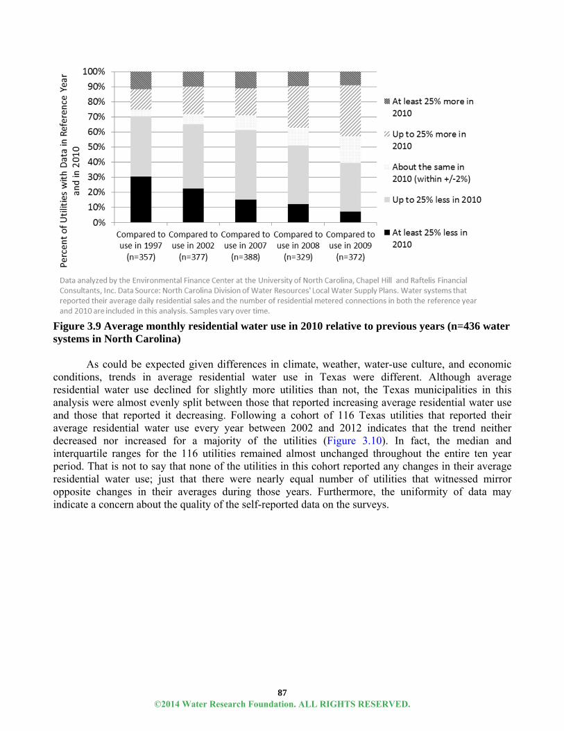
87
Figure 3.9 Average monthly residential water use in 2010 relative to previous years (n=436 water systems in North Carolina)
As could be expected given differences in climate, weather, water-use culture, and economic conditions, trends in average residential water use in Texas were different. Although average residential water use declined for slightly more utilities than not, the Texas municipalities in this analysis were almost evenly split between those that reported increasing average residential water use and those that reported it decreasing. Following a cohort of 116 Texas utilities that reported their average residential water use every year between 2002 and 2012 indicates that the trend neither decreased nor increased for a majority of the utilities (Figure 3.10). In fact, the median and interquartile ranges for the 116 utilities remained almost unchanged throughout the entire ten year period. That is not to say that none of the utilities in this cohort reported any changes in their average residential water use; just that there were nearly equal number of utilities that witnessed mirror opposite changes in their averages during those years. Furthermore, the uniformity of data may indicate a concern about the quality of the self-reported data on the surveys.
©2014 Water Research Foundation. ALL RIGHTS RESERVED.

88
Figure 3.10 Average residential water use among 116 municipalities in Texas from 2002 to 2012
Figure 3.11 displays the changes in average residential water use between 2002 and 2012 for 423 Texas utilities. Based on the self-reported data, average residential water use declined for a larger portion of utilities between 2002 and 2012.
©2014 Water Research Foundation. ALL RIGHTS RESERVED.

89
Figure 3.11 Percentage changes in average household water use for 423 Texas municipal water utilities, 2002-2012 (self-reported)
When analyzed on a year-to-year basis, Texas utilities were more likely to report stable or increasing water use trends, especially in later years, than were their counterparts in the national and North Carolina data sets, reinforcing the importance of trends in water use practices across the country. For example, in many parts of Texas, outdoor watering around the foundation of a house is viewed as an essential water use to prevent structural foundation damage due to rapidly shrinking and shifting clay soils. This water use practice may be viewed differently than outdoor watering in other parts of the country to maintain green grass.
Furthermore, the median average residential water use in Texas is higher than it is in North Carolina: about 6,000 gallons/month versus less than 4,500 gallons/month, respectively. Analysis shown in the Trends in Pricing section indicate that water rate increase amounts and frequencies are very similar in Texas and North Carolina, implying that rate increases may not be the driving factor for the differences in water use trends between the states while variations in the climate and water availability in the two states likely are, in addition to other regional differences. The Impact of Weather and Droughts
A major external driver behind customer water demand (and ultimately utility revenues) is weather. In suburban communities where residential and non-residential customers irrigate lawns and landscapes during the summer, the seasonal demand for water is highly dependent on precipitation and temperature patterns. During rainy summers, customers are likely to significantly curtail their outdoor water demand. In summers with warmer temperatures than normal, water demand might increase as customers use more water for cooling towers, irrigation, filling swimming pools, etc. The relationship between precipitation, temperature, and water demand are not always clear cut, though, since different
3%
11%
8%
17%
8%
23%
17%
11%
3%
0%
5%
10%
15%
20%
25%Percentageof423TexasMunicipalWater
Utilities
©2014 Water Research Foundation. ALL RIGHTS RESERVED.

90
combinations of precipitation and temperature patterns may affect customer demands in unpredictable ways. Nonetheless, utilities in which water demand cycles with the seasons will usually find that high-season water demands, and therefore water sales, will vary from year to year at least partly in accordance to weather patterns.
To complicate the relationship even further, long-term weather patterns and climate change may create changing conditions that affect customer demands for some utilities. One way long-term trends in precipitation and temperature manifest themselves at the local level is in creating droughts. During droughts, water demand patterns will change. On the one hand, temperatures and precipitation patterns during droughts are usually such that water demand increases as customers purchase more water for irrigation and cooling purposes. This was recognized in the Fitch Ratings’ Special Report on the financial impact of Texas’ 2011 drought, for example, reporting that droughts can improve the financial conditions of utilities with ample supplies that do not have to enact water use restrictions because customer demands increase, leading to greater revenues (Scott et al. 2011).
On the other hand, when droughts sufficiently diminish utilities’ water supplies, utilities often attempt to lower their customers’ demands through conservation programs, pricing, and use-restrictions in order to ensure sufficient water resources are available for the most basic needs of all customers. By implementing demand-side management strategies, utilities may be successful in lowering customer demands during water shortage periods, but the decreasing demands translate to decreasing revenues for the utilities. As explained previously, the majority of the utilities’ expenses, at least in the short-run, are fixed while the majority of revenues are obtained from the commodity charges. As customers conserve, utility revenues decline much faster than utility expenses. Some utilities may offset the revenue losses due to conservation during water shortage periods by implementing “drought surcharges.” Overall, therefore, droughts and long-term weather may affect utilities’ finances either positively or negatively, depending on local conditions.
Across the United States, drought conditions are assessed and monitored weekly in the U.S. Drought Monitor, which is produced in partnership between the National Drought Mitigation Center at the University of Nebraska-Lincoln, the United States Department of Agriculture, and the National Oceanic and Atmospheric Administration (U.S. Drought Monitor 2013). The Drought Monitor synthesizes multiple indices that measure drought conditions using historic weather data into a single, categorical value:
Normal: no drought D0: abnormally dry D1 drought: moderate D2 drought: severe D3 drought: extreme D4 drought: exceptional
©2014 Water Research Foundation. ALL RIGHTS RESERVED.

91
Figure 3.12 shows the percentage of area in the United States and Puerto Rico under various levels droughts weekly between January 2000 and February 2013. During this 12 year period, 7% - 55% of the area was in D1 – D4 levels of drought in any one week. Droughts were more significant in 2002-2004, 2006-2007, and from 2011 onwards, when at least 10% of land was in extreme or exceptional drought. Such high drought prevalence, particularly for extreme droughts, is indicative of the need for utilities to develop effective water shortage response strategies (and corresponding revenue response strategies) that will help maintain utility financial health in case conservation programs are enacted.
Figure 3.12 Percent area in the United States and Puerto Rico in different stages of drought between January 2000 and February 2013 Water Use, Rates, and Revenue
Could increasing water prices also be behind the nation’s shift in water demand? Although Consumer Price Index increased by only 22% between 2004 and 2012, a national cohort of utilities raised rates by a median 50% during that same time period. Likewise, our research indicates that the majority of utilities in six states have been raising rates faster than the rate of inflation in recent years. Though many of the utilities are likely raising rates to shore up their financial position and/or to promote conservation through pricing, it is also possible that the rate increases have been both a cause and a result of decreasing consumption.
As water use falls, if rates and pricing structure is not altered, revenues decline substantially faster than utilities’ costs, which are mostly fixed. In a falling use environment, utilities must raise customer’s bills and unit prices to maintain revenue generation at a level sufficient to pay for the (mostly fixed) costs of the utility. These higher rates, in turn through price elasticity, increase the financial incentive for customers to conserve, leading to further water use declines. The magnitude of this effect is highly dependent on the price elasticity of demand for drinking water. The more a utility raises its rates, the more price sensitive customers may become when their water and wastewater
©2014 Water Research Foundation. ALL RIGHTS RESERVED.

92
charges comprise larger portions of their monthly budgets. Utilities must therefore be careful in using rate increases to cope with lost revenue from falling consumption. If rate calculations do not take into consideration falling usage adequately, the utility may be forced to implement additional unplanned for rate increases.
If water rates do not go up, declining use might be expected to take water utility revenue with it. Figure 3.11 graphs the change in average water use per-account versus the percent change in operating revenues per account for 96 utilities between 2010 and 2012. The analysis shows a definite positive correlation between changes in average water use and changes in operating revenues. But it also shows that revenues have been partly resilient to water use. In many cases, revenue changes were above the 1-to-1 line, indicating that changes to operating revenues were greater in value than changes to average water use. This is good news for utilities. A 10% decline in average water use results in less than a 10% decline in revenue. Although, there were a few utilities whose increases in average water use did not seem to drive corresponding increases in revenues. Conclusion
Whether the result of changes in rates, weather, household size, efficiency policy, economic realities, or a combination of all and then some, lower levels of water use per customer is likely to represent a “new normal” for water utilities. It may be unlikely for water use to return to prior levels, given the ever-increasing efficiencies of water appliances and fixtures, and due to continual pressure to conserve both due to ever-increasing rates and a growing conservation ethos among customers. Data indicate that water use declines have been occurring for several years. In the long-run, these reductions are beneficial to the utility and to the environment, putting less stress on existing water resources, lowering power and chemical uses and costs, delaying the need for expanding water resource supplies, freeing current supplies for future customers, and preserving water resources for environmental uses. However, because demand is closely linked to utility revenue, low levels of water use in the short-run are likely to create the largest financial challenge facing water and sewer utilities in the coming decade. Our analysis shows that in the recent past, utilities have been able to maintain and even increase revenue levels despite trends in declining demand. Regardless, future strategies should focus on maintaining revenue stability and financial solvency in the context of lower demand. At the very least, utilities should strive for detailed, integrated, and updated demand forecasts (explained in the Strategy Section of this report) when projecting costs and revenues and setting rates for upcoming years. References Boyle, C. M. Tiger, M. Ngo, S. Eskaf and C. Wichman. 2012. Shifting Baselines in Water
Management: Using customer-level analysis to understand the interplay between utility policy, pricing, and household demand. Chapel Hill, N.C.: Environmental Finance Center. [Online]. Available: <http://www.efc.unc.edu/publications/2012/ShiftingBaselines.pdf>. [cited May 23, 2012]
DeOreo, W.B. and P.W. Mayer. 2012. Insights into declining single-family residential water demand. Jour. AWWA, 104(6): 383–394.
Rockaway, T.D., P.A. Coomes, J. Rivard and B. Kornstein. 2011. Residential water use trends in North America. Jour. AWWA, 103(2): 76-89.
Scott, D., G. Gutierrez, J. Seebach, and T. Wenck. 2011. Fitch Ratings Special Report: Texas-Sized Drought for the Lone Star State. New York, N.Y.: Fitch Ratings.
U.S. Drought Monitor. 2013. Current U.S. Drought Monitor. [Online]. Available: <http://droughtmonitor.unl.edu/ > [cited February 16, 2013]
©2014 Water Research Foundation. ALL RIGHTS RESERVED.
93
ECONOMIC CONDITIONS Introduction
The water and wastewater industry has long relied on the conventional wisdom that everyone needs water services, and that while the cost is increasing, the services are still priced at reasonable enough levels that customer ability-to-pay is not a major hurdle to resiliency of the existing business model. This section includes an analysis of the economic conditions facing residential and non-residential water and wastewater customers to characterize the stress changing economic conditions may be placing on revenue generation for utilities.
Economic conditions have the potential to influence a utility’s financial condition in a number of different ways. As issuers of debt and consumers of goods and services, utilities’ expenses are subject to economic conditions, through changing availability and terms of debt and changing prices of labor and materials. But economic conditions can also influence utility revenues. When residential customers experience economic difficulties through declining income and rising unemployment, their ability to pay for water and wastewater services diminishes and the customers may be more likely to reduce their expenditures on these services through reduced consumption. Likewise, commercial and industrial customers that are negatively affected by economic conditions may seek to cut costs by reducing water consumption or even installing wells to lower their water expenditures. In worst cases, a decline in the economic conditions may force small businesses and industries to close or leave town, completely eliminating their portion as a source of revenue to the water and wastewater utility. As shown in the Service Area Size and Diversity Section, some utilities rely heavily on their largest five customers for a substantial portion of their total revenues; should one or two of these customers leave, the utility will be hard-pressed to make up the loss in revenues from their other customers. Additionally, a slowdown in the growth in a utility’s service area means that there will be fewer new customers that would connect to the utility and pay the connection (tap) and system development (impact) charges, deposits, account activation charges, etc. (Although, the loss of these revenues may be offset by a reduction in the expenses of extending pipes to those new customers.)
In addition to driving down demand and growth-associated revenue, a weak economy can negatively influence a utility’s capacity to increase pricing. In a special report, Standard & Poor’s observed that the annual increase in water utility rates far outpaced even the most optimistic projections in the change of real disposable income (Chapman, Breeding, and Buswick 2013). Our own analysis indicates that water and wastewater rate increases have generally outpaced inflation of the Consumer Price Index since 2008, indicating that the charges for water and wastewater service have risen much faster than the rise in other consumer goods. Nonetheless, governing boards of local governments are challenged to balance all rate and tax increases within their control (e.g. water and wastewater rates, property taxes, fees, etc.) and the financial conditions outside of it. In difficult economic times, governing boards may choose to stagger increases to different services over time instead of raising costs to their citizens on multiple fronts. Investor-owned utilities and wholesalers must also stay sensitive to their customers’ ability to pay. Key Points
With worsening economic conditions, many residential and non-residential customers’ incomes have generally decreased or remained stagnant, while the cost of water and wastewater services has increased.
A bad economy, so far, has not resulted in a drastic fall in revenues, but has resulted in much more affordability pressure in many utilities.
©2014 Water Research Foundation. ALL RIGHTS RESERVED.

94
In some cases, declining economic conditions also have direct immediate impacts on revenues, for example, our analysis shows a strong relationship between trends in new home construction and connection charge revenue.
Ultimately, utilities across North America operate in very different economic environments with very different pressures. These pressures must be considered in developing business strategies.
Trends in Economic Conditions
Recent trends in economic indicators likely to influence a utility’s operating revenues are shown in Figures 3.13-3.16. Figure 3.13 tracks the unemployment rate of all persons aged 16 or over across the United States and Puerto Rico. Figure 3.14 shows the percentage of people living in poverty between 2000 and 2011. Figure 3.15 shows the median household income in the same time period in real terms, adjusted to 2011 dollars. Figure 3.16 shows the change in housing units started across the country and by region between 2000 and 2012. In all four graphs, it is clear that socioeconomic and housing conditions have worsened since 2000, and the effects of the recession after 2008 are sharply on display. In Figure 3.13, the national unemployment rate increased from 4.0% in January 2000 to 7.8% in December 2012. The national unemployment rate doubled (by five percentage points) during the “Great Recession” between April 2008 and October 2009. While the unemployment rate has declined since then through December 2012, unemployment remained at twice the level it was in January 2000.
Figure 3.13 Monthly unemployment rate in the United States Among People 16 Years and Over, January 2000 – December 2012
This rise in unemployment led to a corresponding rise in poverty and decline in income, as
shown in Figures 3.14 and 3.15. The national poverty rate increased from 11.3% in 2000 to 15.0% in 2011. In the seven states that this research focuses on, poverty rates increased in all states, by 1.9 – 6.3 percentage points during the same time period.
©2014 Water Research Foundation. ALL RIGHTS RESERVED.

95
Figure 3.14 Percent of people in poverty, 2000 to 2011
At the same time, the median household income decreased across the United States and in all seven states since 2000 when adjusted to 2011 dollars, as shown in Figure 3.15. The nationwide median household income decreased by nearly $5,000 (8.7%) over the eleven year period, with three focus states seeing a decrease of more than $7,500. In other words, more than half of the households in the country made at least $5,000 less in 2011 than in 2000 in terms of real dollars. Thus, households across the country, in general, had decreasing purchase power between 2000 and 2011, while experiencing a 33% increase in consumer prices and an even larger increase in water and wastewater rates post-2008. There are regional differences in how the economic conditions affected households. In Figures 3.14 and 3.15, the States of Ohio and Georgia witnessed the greatest decreases in median household income and greatest rises in poverty rates since 2000, whereas the changes in the State of Texas were minor by comparison. There exist also significant differences in socioeconomic conditions between states in 2011 alone, with median household incomes ranging across the seven states between $45,206 in North Carolina and $58,629 in Colorado.
Figure 3.15 Median household income in 2011 dollars, 2000-2011
©2014 Water Research Foundation. ALL RIGHTS RESERVED.

96
Figure 3.16 tracks the number of housing units started across the nation since 2000, as well as in regions of the country. The impact of the recession is most drastically seen in this graph. The U.S. Southern and Western regions experienced the largest decline in housing units started over the twelve-year time period, when housing units started falling by almost 50% in both regions. The Northeast and Mid-west also experienced declines, also to a more modest degree.
Figure 3.16 Housing Units Started Nationally and By Region, 2000-2012
The relationship between changing economic conditions at the local (county) level and the
financial performance of combined water and wastewater utilities is demonstrated in Figures 3.17 – 3.19. Using biennial income statement data from 2004- 2012 compiled for the national AWWA-RFC Water and Wastewater Rates Surveys, 143 utilities in 41 states with financial data in two separate years at least 4 years apart were identified and used in this analysis. The combined water and wastewater operating revenues was divided by the number of accounts served by the utility in the two years and used to calculate the percent change in average operating revenue per account between the two years. Each utility was matched to a county, and the county’s statistics on average annual unemployment rate, poverty rate, and median household income for the equivalent years were obtained from the U.S. Bureau of Labor Statistics and the U.S. Census Bureau. The change in the values of these three local economic indicators between the two years were then computed and graphed against the change in the average operating revenues per account, shown in Figures 3.17 – 3.19. Each dot represents one of the 143 utilities, and the trend line is added to each graph.
No significant correlations were observed in any of the three indicators with changing operating revenues per account, and the trend lines were only very slightly positive (but not statistically significant). In all three graphs, it is clear that the 143 utilities experienced very different changes to economic conditions and operating revenues. Although economic conditions in the United
DataanalyzedbytheEnvironmentalFinanceCenterattheUniversityofNorthCarolina,ChapelHillandRaftelisFinancialConsultants,Inc.Datasource:U.S.CensusBureau,BuildingPermitsData,NewResidentialConstruction
DataanalyzedbytheEnvironmentalFinanceCenterattheUniversityofNorthCarolina,ChapelHillandRaftelisFinancialConsultants,Inc.Datasource:U.S.CensusBureau,BuildingPermitsData,NewResidentialConstruction
©2014 Water Research Foundation. ALL RIGHTS RESERVED.

97
States worsened over time, only 39 out of the 143 utilities (27%) experienced a decrease in average operating revenues per account between their two years of analysis, despite decreasing demands, mostly as a result of increased rates. The majority of the utilities, therefore, increased their operating revenues per account over time.
In Figure 3.17, 92% of the utilities were in counties that experienced an increase in the local unemployment rate all the way up to a 12.7 percentage point increase for one utility between 2008 and 2012 (City of Yuma, AZ). In Figure 3.17, 92% of the utilities also experienced an increase in the county’s poverty rate all the way to a 10.1 percentage point increase between 2004 and 2012 for the City of Ames, IA. In Figure 3.18, 72% of the utilities witnessed the local median household income, in 2012 dollars, decrease in their county. Changes to the counties’ median household incomes ranged from a decrease of 17.5% between 2006 and 2012 in Waterford, MI and an increase of 14.3% between 2004 and 2012 in New York City, NY. These trends signify that the local economic conditions worsened over time for a large majority of the 143 utilities in 41 states, as expected. With worsening economic conditions, residential and non-residential customers’ ability to pay for water and wastewater services may have generally decreased.
Rate increases allowed three-quarters of the utilities to collect more revenues per account over time, aiding the utilities’ financial performance and demonstrating that water services in most areas display a certain level of inelasticity. Along with findings in the Trends in Financial Performance (Chapter 2) that total operating revenues also generally increased from 2000 to 2012, these findings imply that the worsening economic conditions of the past decade have not completely eroded utility revenues, as is likely to have occurred in certain sectors during the downturn (e.g. tourism revenues). On the other hand, collecting more revenues per account, while the customers’ ability-to-pay for services decreases over time, means that utility rates are becoming less affordable. However as shown in Figures 3.17 – 3.19, increased unemployment, increased poverty, and decreases in income do not, on their own, equate to utility revenue troubles. However, they do provide insight into the different operating environments facing utilities. Clearly, some areas of the country have customer bases with economic conditions severe enough to potentially impact customers’ abilities to pay for services, even essential services.
Figure 3.17 Changes in average combined water & wastewater operating revenues per account and the county’s unemployment rate over at least a 4-year period for 143 utilities nationwide.
©2014 Water Research Foundation. ALL RIGHTS RESERVED.

98
Figure 3.18 Changes in average combined water & wastewater operating revenues per account and the county’s poverty rate over at least a 4-year period for 143 utilities nationwide
Figure 3.19 Changes in average combined water & wastewater operating revenues per account and the county’s median household income over at least a 4-year period for 143 utilities nationwide.
Average expenditure for water and/or wastewater services portrayed as a percentage of median household income (MHI) continues to be widely used to provide a snapshot of affordability pressure within a particular community or service area. This metric is only able to present a limited view of household-level challenges. The denominator of the indicator MHI is plagued with shortcomings as an indicatorit masks income distribution within a community and discounts the low-income part of a community curve. A single parent family with two children who makes just over minimum wage will
©2014 Water Research Foundation. ALL RIGHTS RESERVED.

99
earn less than $20,000 per year. These types of distressed families make up a portion of almost every community, regardless of the community’s median income. Both a community with an MHI of $75,000 or one with an MHI of $30,000 will experience the same affordability challenge related to this type of low-income family. Addressing the financial impacts of water service on low-wealth families is both a public policy issue and a financial issue; as distressed families have more difficulty paying bills, the amount of late payments and disconnections go up. In addition, as it becomes clear that some families are unable to pay for basic services, the pressure on elected boards to keep rates low for the entire customer base increases.
Figure 3.20 shows the evolution of water and wastewater expenditures between 2004 and 2012 using two metrics. The chart on the left shows that almost every utility in the sample asked their customers to pay a greater percent of their income on water services in 2012. The data also show that even though the percent of income devoted to water has increased, it still remains below 2% for all of the utilities. The right side of the chart shows the evolution of the percentage of household income a family with an income at poverty threshold pays within the same utility sample. The analysis shows much more significant changes facing low income families with many families that had been paying less than 2% of their income, now paying 3% or higher.
Figure 3.20 Comparison of the cost of water as a percent of median household income and as percent of poverty threshold
©2014 Water Research Foundation. ALL RIGHTS RESERVED.
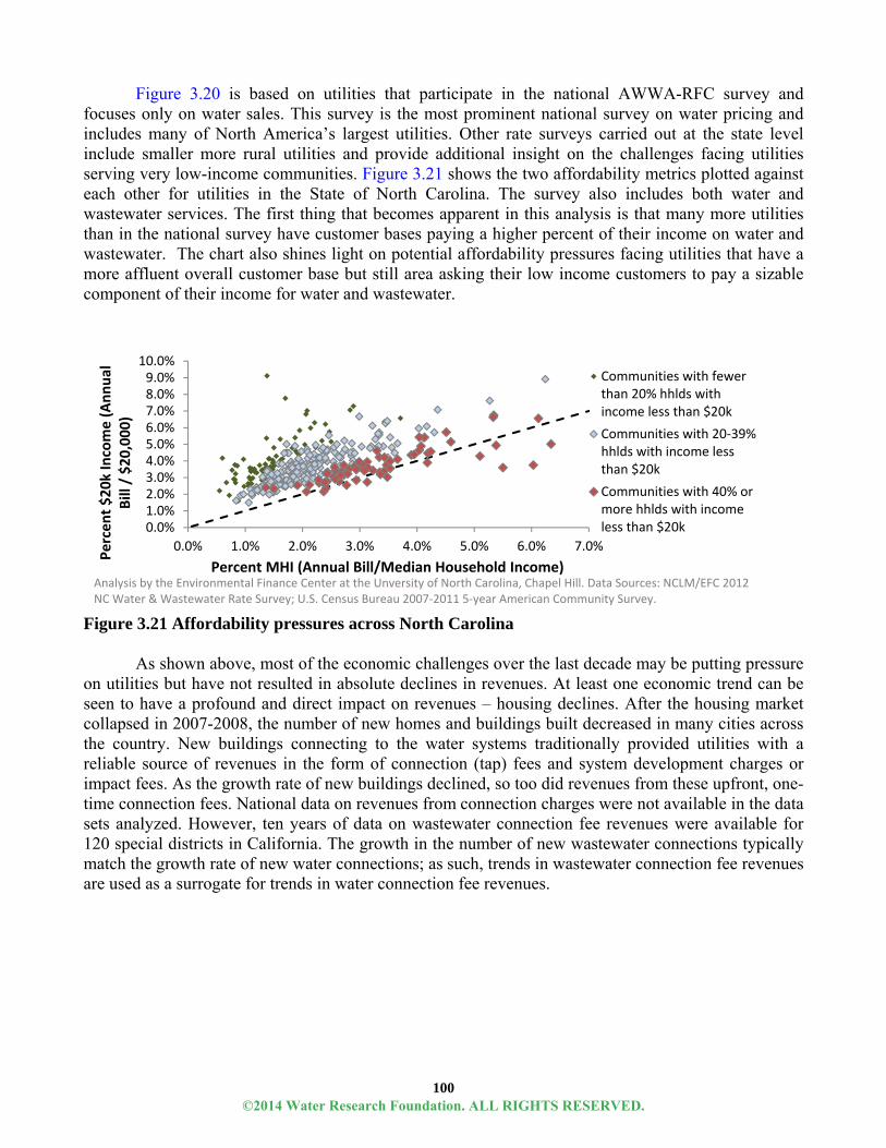
100
Figure 3.20 is based on utilities that participate in the national AWWA-RFC survey and focuses only on water sales. This survey is the most prominent national survey on water pricing and includes many of North America’s largest utilities. Other rate surveys carried out at the state level include smaller more rural utilities and provide additional insight on the challenges facing utilities serving very low-income communities. Figure 3.21 shows the two affordability metrics plotted against each other for utilities in the State of North Carolina. The survey also includes both water and wastewater services. The first thing that becomes apparent in this analysis is that many more utilities than in the national survey have customer bases paying a higher percent of their income on water and wastewater. The chart also shines light on potential affordability pressures facing utilities that have a more affluent overall customer base but still area asking their low income customers to pay a sizable component of their income for water and wastewater.
Figure 3.21 Affordability pressures across North Carolina
As shown above, most of the economic challenges over the last decade may be putting pressure on utilities but have not resulted in absolute declines in revenues. At least one economic trend can be seen to have a profound and direct impact on revenues – housing declines. After the housing market collapsed in 2007-2008, the number of new homes and buildings built decreased in many cities across the country. New buildings connecting to the water systems traditionally provided utilities with a reliable source of revenues in the form of connection (tap) fees and system development charges or impact fees. As the growth rate of new buildings declined, so too did revenues from these upfront, one-time connection fees. National data on revenues from connection charges were not available in the data sets analyzed. However, ten years of data on wastewater connection fee revenues were available for 120 special districts in California. The growth in the number of new wastewater connections typically match the growth rate of new water connections; as such, trends in wastewater connection fee revenues are used as a surrogate for trends in water connection fee revenues.
0.0%1.0%2.0%3.0%4.0%5.0%6.0%7.0%8.0%9.0%10.0%
0.0% 1.0% 2.0% 3.0% 4.0% 5.0% 6.0% 7.0%Percen
t $20
k Income (Ann
ual
Bill / $2
0,00
0)
Percent MHI (Annual Bill/Median Household Income)
Communities with fewerthan 20% hhlds withincome less than $20k
Communities with 20‐39%hhlds with income lessthan $20k
Communities with 40% ormore hhlds with incomeless than $20k
Analysis by the Environmental Finance Center at the Unversity of North Carolina, Chapel Hill. Data Sources: NCLM/EFC 2012 NC Water & Wastewater Rate Survey; U.S. Census Bureau 2007‐2011 5‐year American Community Survey.
©2014 Water Research Foundation. ALL RIGHTS RESERVED.

101
As shown in Figure 3.22, revenues from wastewater connection fees generally increased from FY2001 to FY2008 in California, before sharply declining. The median revenues from wastewater connection fees in FY2010 were 74% lower than the median revenues just two years prior. The interquartile range of revenues in the cohort also decreased significantly since FY2008, declining by 49%-68% in two years. If these trends were similar to trends in declining revenues from water connection fees, utilities that had been relying on new connections as a significant source of revenues each year would have seen these revenues virtually disappear, leaving them with a financial gap in the absence of increased rates.
Figure 3.22 Revenues from wastewater connection fees from FY2001 to FY2010 for the same 120 California special district utilities
These trends are also noticeable at the utility-level, as shown in Table 3.3. Water (and wastewater) tap fee revenues from seven Colorado utilities declined significantly since between FY2008 and FY2010. As shown by the sparklines, the tap fee revenues decreased by more than half in the span of a few years. Since 2010, the housing market has partially recovered, suggesting that revenues from connection fees and system development charges may be increasing once again. However, national and statewide data are not yet available to verify.
©2014 Water Research Foundation. ALL RIGHTS RESERVED.

102
Table 3.3 Tap fee revenues for seven Colorado utilities, FY2004 – FY2010
References
Chapman, T., J. Breeding and G. Buswick. 2013. U.S. Municipal Water and Sewer Utilities Face Continued Rate and Drought Pressure in 2013. Dallas, Tex.: Standard & Poor’s Rating Services.
CAPACITY UTILIZATION Introduction
One of the most important decisions a utility controls is when and how to expand capacity as their customer demands evolve with time. Typically, as demand grows and water production or transmission nears the capacity of a utility’s system, facilities are expanded to meet anticipated demands far into the future. Immediately after the major expansion of a critical facility such as a treatment plant, the system will likely have underutilized capacity for years to come. The larger the treatment plant expansion, the greater the initial cost, but the longer it takes before additional expansions are required.
Utilities that are nearing capacity have several alternatives including: installing new capacity that will serve them for many years to come; investing in conservation programs to extend existing capacity; and/or sharing unused capacity from nearby utilities. The threat of running out of capacity typically dominates the decision process for many utilities despite the financial cost of underutilized capacity. For most, the political impact of failing to meet demand is far greater than the financial cost. Key Points
Utility capacity (as measured as a function of water treatment plant capacity utilization) varies significantly among individual utilities; the majority of utilities use 50-80% of their capacity on a maximum day.
No clear, direct relationships appeared between capacity utilization and rates of return on equity, but more in-depth analysis is expected to reveal a detrimental financial impact with building capacity necessary to meet overestimated demands.
FY'04 '05 '06 '07 '08 '09 '10City of Florence's water tap fee revenuesCity of Grand Junction Water's water tap fee revenuesBuena Vista Sanitation District's sewer tap fee revenuesCherokee Metropolitan District's water & sewer tap fee revenuesCity of Brighton's water & sewer tap fee revenuesCity of Broomfield's sewer tap fee revenuesCity of Fruita's sewer tap fee revenues
Percent change in tap fee revenues from previous
Fiscal Year
Tap fee revenues FY2003-FY2010
Utility in Colorado
Data analyzed by the EnvironmentalFinance Center at the University of North Carolina, Chapel Hill and Raftelis Financial Consultants, Inc. Data Source: Colorado Water Resources and PowerDevelopment Authority. Bars reflect the percent change
to annual revenues from tap fees from previous fiscal year. Dark bars are relative gains, light bars are relative losses. The y‐axis scales are unique for each utility.
©2014 Water Research Foundation. ALL RIGHTS RESERVED.

103
Utilization rates influence what types of management practices utilities can employ to improve their financial position.
Assessing Capacity Utilization
In an effort to explore the relationship between capacity utilization and financial performance, two different data sets of self-reported information on water utilities’ treatment capacity, daily usage, pricing, and financial performance were used. The first dataset comes from a biennial survey of North American utilities conducted by the American Water Works Association (AWWA) and Raftelis Financial Consultants, Inc. (RFC) and includes information from 570 utilities throughout the United States and Canada for the years from 2000 through 2012. The second data set comes from the State of North Carolina’s Local Water Supply Plans (LWSP). These plans are submitted to the state’s Department of Environment and Natural Resources by all local government-owned and all large community water systems in the State and contain information on their water sources, sales, and treatment plants. These data sets were merged with utility rate data from the North Carolina League of Municipalities (NCLM) and the Environmental Finance Center at the University of North Carolina (EFC) annual rates surveys and financial reports from the North Carolina Office of the State Treasurer.
Unfortunately, data were not available to factor in excess capacity in the pumping and distribution system. Capacity Utilization Trends The water treatment plant capacity for utilities participating in the AWWA-RFC survey was assessed against systems’ average and maximum days2. Using AWWA-RFC figures for 2012, the median average day sales as a percent of capacity was 38%. The median maximum day sales as a percent of capacity were 68%. The full distribution, shown in the Figure 3.23, shows the majority of utilities between 20-40% capacity utilities on an average day and between 50-80% capacity utilization on a maximum day. Utilities with treatment facilities in North Carolina followed a similar distribution.
2 This analysis also revealed an underlying challenge in working with self-reported data. A small subset (less than 5%) of utilities responding to the
AWWA-RFC survey reported maximum and, in some cases, average-day water usage that was significantly higher than their plant capacity. Though the survey asks for “max-day water production” and “daily water treatment production capacity,” it seems clear that many utilities responded with figures that reflected more than just what is happening at their treatment plant. For example, one utility in California reported that it had a daily production capacity of 24 million gallons, but that it produced 44 million gallons on its peak day in 2010. The utility’s operating statistics for fiscal year 2010-2011 show, by contrast, that it actually has a combined treatment plant capacity of only 9 million gallons daily. Water purchases from another utility make up the bulk of its remaining source of drinking water. This underlying ambiguity in the AWWA-RFC survey response inhibits the ability to produce more extensive analyses from some utilities’ capacity utilization estimates.
©2014 Water Research Foundation. ALL RIGHTS RESERVED.

104
Figure 3.23 Plant capacity utilization in 2012 of 251 water utilities Across North America
Over the past twelve years, the AWWA-RFC survey sample reports minimal changes in average day capacity utilization. As shown in Figure 3.24, utilities responding to the survey in 2000 reported median average-day capacity use of 41%. That figure rose to 42% in 2002 and again in 2006 before declining to a median average-day capacity utilization of 38% in 2012.
Figure 3.24 Average day capacity utilization from 2000-2012 for water utilities across North America
©2014 Water Research Foundation. ALL RIGHTS RESERVED.

105
While the median capacity utilization rate across the sample has stayed relatively steady, individual utilities have seen more pronounced trends. Figure 3.25 shows the trend for the sub-group of 25 utilities that responded to each of the seven AWWA-RFC surveys. Those utilities experienced regular increases in their plant capacity (approximately 15% over the 12-year period), even though their average and maximum day use fell by an average of approximately 10% during the same timeframe. In other words, these 25 utilities expanded their treatment plant capacities during a time when their total demands were actually decreasing. Financially, this likely placed additional burdens on the utilities and their customers to pay for the new capital costs and associated higher operating and maintenance costs, while collecting lower revenues as customers use less water.
Figure 3.25 Change in plant capacity and water use over time for 25 utilities Relationship Between Treatment Plant Capacity Utilization and Utility Financial Condition
But to what extent do these trends impact the actual financial condition of a utility? To provide an initial take on this question, utilization rates were studied against water charges and a financial indicator; the results used to discuss the various finance and management options available to utilities in different circumstances. Capacity utilization was plotted against the household charge at a standardized consumption level to detect if utilities with underutilized capacity have higher charges than their peers. Additionally, capacity utilization was also plotted against a utility’s return on assets (operating revenues divided by total assets) to assess the financial efficiency of operating at a higher capacity. Ultimately, neither of these methods provided conclusive results on the direct relationship between capacity utilization and charges or financial performance, but rather suggests a more complex relationship between external drivers and strategies that can be engaged for utilities at either end of the spectrum.
©2014 Water Research Foundation. ALL RIGHTS RESERVED.

106
Household charge When examined in isolation, water treatment plant capacity utilization did not have a direct relationship with household charge (as shown in Figures 3.26 and 3.27). In other words, utilities with lower or higher plant capacity utilization did not necessarily have predictable lower or higher rates. Each figure plots a calculation of capacity utilization on a system’s maximum day (National utilities, Figure 3.26) and a system’s average day (North Carolina utilities, Figure 3.27). Even though, there is no clear trend between capacity utilization and the absolute charge at one consumption point, these graphs do allude to differences in system characteristics and pricing challenges and opportunities for utilities. For example, the utility in Figure 3.26 that has low maximum-day capacity utilization but relatively high water charges should hope to sell wholesale water to a neighboring community or experience rapid community growth to cover the costs of this capacity. Meanwhile, a utility with high water charges and high capacity utilization may have proactively increased rates to cash-finance a portion of the high capacity.
Figure 3.26 Water charge at 10 ccf and maximum day capacity utilization in 2012 for 241 National utilities
$0
$10
$20
$30
$40
$50
$60
$70
$80
0 20 40 60 80 100 120
Water Charge at 10ccf
Maximum Day Capacity UtilizationDataanalyzedbytheEnvironmental FinanceCenterattheUniversityofNorthCarolina,ChapelHilll.Waterchargerepresentseitheryear‐roundratesortheaverageofhighandlowseasonrates.Datasource:FinancialandoperatingdatacompiledbyRaftelisFinancialConsultants.
©2014 Water Research Foundation. ALL RIGHTS RESERVED.

107
Figure 3.27 Water charge at 7,000 gallons and average day capacity utilization in 2011 for 176 North Carolina utilities Return on Assets
Despite the fact that utilities are monopolies, theoretically, a system that is “optimizing” its capacity should be generating a higher return on those assets than a utility with underutilized capacity. Figures 3.28 and 3.29 show that utilities with higher capacity use on both the maximum and average day did tend to have slightly higher returns, but there is still a great deal of variation in the data, indicating that a number of other factors are playing into a utility’s return on its assets (operating revenue divided by total assets).
Figure 3.28 Return on assets and maximum day capacity utilization in 2012 for 212 national water utilities
$0
$20
$40
$60
$80
$100
$120
0 20 40 60 80 100 120
Water Charge at 7,000 Gallons
Average‐Day Capacity UtilizationDataanalyzedbytheEnvironmental FinanceCenterattheUniversityofNorthCarolina,ChapelHilll.Datasource:UNCEFCWaterandSewerratessurveysandNCDepartmentofEnvironmentandNaturalResourcesLocalWaterSupplyPlanningdata.
0
0.1
0.2
0.3
0.4
0.5
0.6
0.7
0.8
0.9
1
0 20 40 60 80 100 120
Return on Assets
Maximum‐day Capacity Utilization
DataanalyzedbytheEnvironmental FinanceCenterattheUniversityofNorthCarolina,ChapelHilll.Datasource:FinancialandoperatingdatacompiledbyRaftelisFinancialConsultants.
©2014 Water Research Foundation. ALL RIGHTS RESERVED.
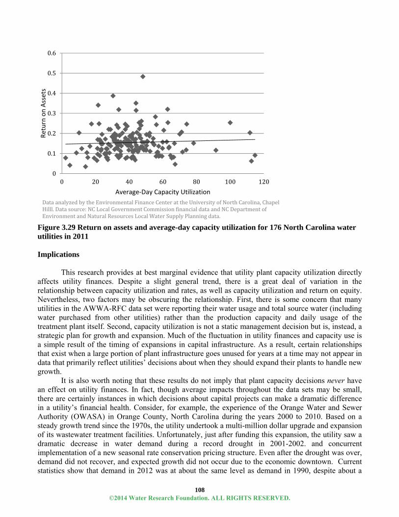
108
Figure 3.29 Return on assets and average-day capacity utilization for 176 North Carolina water utilities in 2011 Implications
This research provides at best marginal evidence that utility plant capacity utilization directly affects utility finances. Despite a slight general trend, there is a great deal of variation in the relationship between capacity utilization and rates, as well as capacity utilization and return on equity. Nevertheless, two factors may be obscuring the relationship. First, there is some concern that many utilities in the AWWA-RFC data set were reporting their water usage and total source water (including water purchased from other utilities) rather than the production capacity and daily usage of the treatment plant itself. Second, capacity utilization is not a static management decision but is, instead, a strategic plan for growth and expansion. Much of the fluctuation in utility finances and capacity use is a simple result of the timing of expansions in capital infrastructure. As a result, certain relationships that exist when a large portion of plant infrastructure goes unused for years at a time may not appear in data that primarily reflect utilities’ decisions about when they should expand their plants to handle new growth.
It is also worth noting that these results do not imply that plant capacity decisions never have an effect on utility finances. In fact, though average impacts throughout the data sets may be small, there are certainly instances in which decisions about capital projects can make a dramatic difference in a utility’s financial health. Consider, for example, the experience of the Orange Water and Sewer Authority (OWASA) in Orange County, North Carolina during the years 2000 to 2010. Based on a steady growth trend since the 1970s, the utility undertook a multi-million dollar upgrade and expansion of its wastewater treatment facilities. Unfortunately, just after funding this expansion, the utility saw a dramatic decrease in water demand during a record drought in 2001-2002. and concurrent implementation of a new seasonal rate conservation pricing structure. Even after the drought was over, demand did not recover, and expected growth did not occur due to the economic downtown. Current statistics show that demand in 2012 was at about the same level as demand in 1990, despite about a
0
0.1
0.2
0.3
0.4
0.5
0.6
0 20 40 60 80 100 120
Return on Assets
Average‐Day Capacity Utilization
DataanalyzedbytheEnvironmental FinanceCenterattheUniversityofNorthCarolina,ChapelHilll.Datasource:NCLocalGovernmentCommissionfinancialdataandNCDepartmentofEnvironmentandNaturalResourcesLocalWaterSupplyPlanningdata.
©2014 Water Research Foundation. ALL RIGHTS RESERVED.

109
60% increase in the number of customer accounts that OWASA serves. As a result, the expanded wastewater treatment capacity was not as necessary as originally anticipated, and OWASA’s current capital improvements plan indicates that the utility expects to have no need to expand its wastewater treatment plant further until at least 2030. OWASA’s falling demand is also visible in AWWA-RFC data on water production capacity, which show that the utility’s average day demand was 53% of its water treatment plant capacity in 2000, but only 34% of capacity by 2010. Following a significant debt issuance in 2004, primarily to fund the upgrade and expansion of the wastewater treatment plant, OWASA’s debt to asset ratio increased to 48%. (It has since declined to a current ratio of 30% as the cost of debt-funded assets has been capitalized.)
Despite this anecdote, industry-wide trends reveal no consistent pattern between capacity trends and utility finances. The experience of OWASA demonstrates that unfortunate timing of plant capacity expansions coinciding with decreasing demands can lead to financial constraints. and upward pressure on rates. More in-depth research that uses standardized and validated data could more easily parse out the actual financial impact of overbuilding capacity to meet overestimated demands.
Additionally, utilization rates influence what types of management practices utilities can employ to improve their financial position. Utilities with excess unused capacity have an incentive to sell more water to current customers and/or to minimize future sales reductions. On the other hand, utilities with relatively little excess capacity and are at the other end of the capacity utilization cycle have an opportunity incorporate and benefit from reduced demand rates. The stakes in maintaining excess capacity should be seen as a significant financial risk and potential burden to utility customers particularly in a period of declining or flat sales. Furthermore, and perhaps most importantly, the incremental costs of carrying excess capacity may erode the ability of a utility to invest in rehabilitation and other non-capacity expansion needs. ECONOMIC REGULATION AND GOVERNANCE Introduction
While many utilities have considerable flexibility and freedom to design their pricing model and implement a wide range of locally customized rates and fiscal policies, for some, there are critical economic regulatory and governance factors that influence fiscal condition and the practices and strategies for improving it.
In most cases, the degree to which a particular utility is regulated in a state depends on the state, the type of utility ownership, and service area characteristics. For example, in most states, investor-owned utilities fall under the jurisdiction and economic regulatory influence of a public service or utility commission. In some states, governmental utilities with particular governance structures or service area attributes are regulated. For example, in the State of Maine, governmental public service districts that provide service in multiple jurisdictions are closely regulated by the Maine Public Service Commission, whereas a city-owned system that serves customers within a single city is controlled by the city council (Maine Revised Statutes 1987). Historically, protecting consumers from the adverse impacts of monopolistic practices has driven economic regulation in North America (Beecher 1997), however some of the emerging pricing regulation can be attributed to more general public policy goals. For example, a few state and regional entities prone to drought or water shortages have begun incorporating pricing guidelines or requirements into their environmental regulations and policies. They are profiled below.
The scope of what is covered by an economic regulatory system varies and may include review and approval of rate modifications, review and approval of significant capital investments, control of specific pricing decisions, or general oversight of financial health.
©2014 Water Research Foundation. ALL RIGHTS RESERVED.
110
This section profiles several different economic regulatory models to illustrate the potential pricing and financial resiliency impact of economic regulation and governance systems. Our analysis focused on North American approaches, however it is important to point out that this is an area of utility management that has been studied extensively overseas (Beecher 1997). For example, the United Kingdom’s water management culture is founded on a national economic regulatory system and regulator (Office of Water, aka OFWAT) that has been the target of study for years and is quite different from the prevailing models found in North America.
Water utilities in the United States fall under varying types of ownership and management: state and federal government agencies, tribes, municipalities, counties, districts, authorities, not-for-profit water associations, investor-owned water companies, international and national corporations, individuals, homeowner associations, and more. By October 2012, the 50,803 active community water systems in the United States were nearly evenly split between those owned by local governments (48%) and those owned by private organizations (47%) (USEPA 2012).
The varying organizational structures create different incentives, opportunities, and challenges for managing utilities’ finances. Understanding the characteristics of each organizational structure is therefore essential for a holistic theory of utility financial health. In this section, several broad types of governance ownership and economic regulatory structures are analyzed ranging from city utility departments to investor-owned utilities. While the discussion below of each type of organizational structure is general, in nature, individual distinctions are rampant. Water utilities that are owned by individuals, homeowner associations, state or federal agencies, and tribes are excluded from this discussion since they represent a very small minority of water systems that set rates and directly charge customers for water service. Key Points
Governance and economic regulatory models can take different forms at varying levels across the country, depending on the state and system type.
The economic regulatory framework guiding a utility can have a major influence in the types of financial practices it can implement.
Areas with economic regulators have very different pricing modification trends than those that are locally regulated.
Economic regulation alone does not necessarily guarantee financial strength or resilience. Public policies, such as monopoly protection and water resource management, influence
financial resilience and limit pricing strategies. At a high level, organizational structures do not seem to have a direct influence on rate setting
or financial performance – negatively or positively. However, a more comprehensive analysis of rate setting trends and financial performance may detect more targeted differences between these various types of utilities.
Future research should more comprehensively study the intended and unintended financial ramifications of external utility economic regulation and governance model structures.
©2014 Water Research Foundation. ALL RIGHTS RESERVED.

111
Municipal/County-Owned Utilities
Utilities owned and operated by a municipality or county experience significant political and financial integration with the broader local government. Public utilities are often set up as a separate department in the city or county government, with a director and staff, and, many times, as a dedicated enterprise fund solely for the water and/or wastewater utility. While most municipal/county-owned utilities may have a stated goal of being financially independent, transfers between the government’s general fund (both in and out) are common and provide an interdependence that does not exist for other utility models. Although water and wastewater utilities are normally managed independently of other local government functions, the governing body of the utility is typically the same group of (usually elected) officials who oversee all other local government functions. While staff typically manage the finances of the water utility, they normally must seek approval of the city council or county commissioners for rate increases and for adjusting certain financial policies. It is important to point out that the council/commissioners are typically also responsible for voting on financial decisions for the police or sheriff’s department, public works, parks and recreation, etc. The competing demands of managing the budgets spanning numerous government functions means that the governing body will have less time to devote specifically to managing water utility finances. These conditions may increase disincentives for some governing bodies to raise water rates or approve expensive capital projects. On the other hand, being ultimately and publicly responsible for the water utility, the threat of being voted out of office for mismanagement incentivizes the governing body members to make prudent financial decisions when necessary. There are varying degrees of this model that range from a utility as a government executive department that is treated as a municipal department for government purposes (i.e. directly compete for General Fund dollars) to a government agency that reports to an independent governing board appointed by the mayor and approved by the City Council or Board of County Commissioners (Seidenstat 2003), with a few options in between.
Independent Authorities and Districts
The later model mentioned above (independent board reporting to City or Council) moves the organization of a water system much closer to the structure of an independent authority or district. Local government utilities may be formed independently of municipalities and counties, representing a middle ground between local government ownership and private corporations. California has led the country in the use of municipal utility districts (Seidenstat 2003). These independent authorities or districts are special units of local government set up with the single purpose of providing water and/or wastewater services in a regional area that may or may not transcend municipal/county/state boundaries. Since they are independent of municipal and county governments, they operate without the possibility of transfers in from or out to a government General Fund and are less likely to have broad taxation authority. These utilities typically also have separate governing boards whose sole purpose is to manage the utility and whose attention will therefore be undivided. The makeup, structure, and powers of the governing boards vary across different types of independent authorities and districts. In many cases, the governing board members are appointed to their positions, limiting the influence of elections on their decision-making.
Private Investor-Owned Companies
Private companies have a greater degree of financial and political independence compared to governmental structures, though they face different incentives and challenges associated with investor ownership. Investor-owned utilities seeking sustainable and predictable profits have a financial incentive to raise rates and lower costs to maximize profits for their investors, but are also almost
©2014 Water Research Foundation. ALL RIGHTS RESERVED.

112
always financially regulated by a Utilities Commission in order to ensure a reasonable but not excessive rate of return on investments.
One of the project’s utility partners, Aqua North Carolina, is an investor-owned utility that is part of the national company - Aqua America. The North Carolina Utilities Commission oversees and regulates rate setting and financial practices for Aqua (NC), as well as other investor-owned water utilities. As is the case in many but not all states, North Carolina’s Utility Commission has no authority or influence over rate setting and finances of government-owned water utilities. Aqua (NC) serves 250,000 residents in 53 counties from 796 separate water systems (Aqua 2013). The concept of “separate water system” refers to a Federal environmental regulatory framework that is often very different than the economic regulatory framework. Aqua (NC) is considered to manage nearly 800 separate systems because the systems are not physically connected, have different sources of water, and subsequently, different Public Water identification numbers under state and federal law. However, from an economic regulation perspective, Aqua NC is one system under shared management. This is important, because Aqua’s pricing strategy, which it believes is a key to its financial resilience, is based on a uniform tariff or consolidated rate approach throughout the vast majority of its service area. In other words, a customer served by a groundwater system in the western part of the state pays generally the same rates as a customer served by a larger surface water system in the central part of the state. The ability for an economically regulated utility to implement this pricing strategy, as well as other pricing strategies, such as allowing decoupling or surcharges, to recover unexpected expenses is controlled by utility commissions in most states.
One of the most important impacts of investor-owned water utility regulation is to encourage the concept of “full cost” pricing where rates are set to cover all of the eligible costs of operating a water system, as well as a rate of return to shareholders. There are often disagreements about what constitutes reasonable costs and rate of return on invested capital, but the economic regulatory framework is founded on having utilities fully cover operating as well as capital costs. Self-regulated governmental water utilities, such as those regulated by city or county boards, may have rates that do not cover all of the financial costs (e.g. depreciation) of utility operation – choosing instead to transfer money from the general fund to make the utility financially whole or even to operate the system at a loss. Investor-owned utilities do not have that option in the long-term.
Another important impact of the investor-owned regulation model relates to the ability of utilities to fund and maintain reserve funds. Non-regulated utilities may determine that revenue stability and/or future capital needs justify raising rates in the short-run to fund reserve funds to benefit financial resiliency long- run. In almost every state3, investor- owned utilities set rates based on historic costs and cannot raise rates solely to fund reserve funds.
Government-Owned Utilities Regulated by a Utility Commission
Commonly, government-owned utility finances are regulated almost exclusively by their governing board. In fact, only three out of 45 states in the United States comprehensively regulate public water systems at the state level: Maine, West Virginia, and Wisconsin (Beecher et al. 1994). In these states, governmental utilities have to follow prescribed rate adjustment processes that influence when and how they can modify rates. The impact of this type of regulatory framework can be quite
3 According to the 1993/1994 NRRI Survey on State Commission of Water Utilities, the Michigan Public Service Commission is the only State Commission that allows rate stabilization reserves.
©2014 Water Research Foundation. ALL RIGHTS RESERVED.

113
pronounced. The Wisconsin Public Service Commission regulates rates, large construction projects, utility finance, regional water supply solutions, rules and practices, and legal compliance for all government-owned water utilities (WI PSC 2013).
This report discusses rate adjustment history across six different states. As Wisconsin is the only state in the group that comprehensively regulates government-owned utilities, the analysis suggests that this type of regulation influences utility rate setting and financial performance. Figure 3.30 below compares the frequency of rate adjustments in five consecutive years. The analysis shows a much higher percentage of utilities in Wisconsin did not change rates or changed them only once over the past five years, as compared to the other states.
Figure 3.30 Frequency of rate adjustments in five consecutive years for six states
This has the potential to lead to larger rate increases, as shown in Figure 3.30 With the
exception of California (see Prop 218 discussion below), average rate adjustments are higher (sometimes significantly) for utilities that change rates only once in five years. In Wisconsin, for example, utilities that increased their rates only once in the five year period had rate increases approximately five times larger than those of utilities that increased their rates on a yearly or almost yearly basis (Figure 3.31). Similarly, utilities that changed their rates nearly every year had a significantly lower average rate adjustment. This trend is similar (if not as pronounced) in NC, OH, TX, and GA.
©2014 Water Research Foundation. ALL RIGHTS RESERVED.

114
Figure 3.31 Average rate adjustment by frequency
The stark difference between rate adjustment trends in Wisconsin compared to the other states
does not necessarily indicate financial insufficiency, but it can. Figure 3.32 compares the non-capital operating ratios utilities in Ohio, Texas, and Wisconsin. (The other three states included depreciation in their operating expenses and so cannot be compared at the same level.) Although the analysis shows that the majority of Wisconsin utilities have operating ratios higher than 1.0 (i.e. they are collecting enough revenues to cover the operations and maintenance of their system), between 12% and 26% of utilities, in any given fiscal year, collected less operating revenues than operating expenses (i.e. operating ratio less than 1.0). Under this type of situation, these utilities would have to use their reserves, transfers and/or non-operating revenues to fill the gap between day-to-day operations and maintenance expenditures and their operating revenues, leaving little to no revenue to cover capital expenses.
Figure 3.32 Non-capital operating ratios1 among the same 1,236 utilities in OH, TX, and WI over time
©2014 Water Research Foundation. ALL RIGHTS RESERVED.
115
Other Types of Economic Regulation and Oversight
Interestingly, the data from Ohio and Texas speak to another type of water utility economic regulation that occurs at the state level outside of utility commissions. The ratios computed in Ohio and Texas were for utilities that had outstanding loans with the Ohio Water Development Agency and the Texas Water Development Board, respectively. These utilities have their financial data reviewed, analyzed, and monitored by these two agencies, which work to ensure that the utilities are in strong financial position to pay back their outstanding debts.
State governments have other mechanisms to oversee the financial health of water systems in their jurisdiction. Over recent years, there has been increasing attention given to the fiscal health and sustainability of local governments in many areas of the country.4 While many state governments may have ultimate responsibility for backstopping troubled local governments, some states such as North Carolina, maintain strong on-going financial oversight of local government utilities that directly impacts fiscal policies and pricing. From within the Office of the NC State Treasurer, the Local Government Commission (LGC) assures local governments are managed in a fiscally responsible manner. The LGC requires submittals of audited financial statements from all governmental utilities and reviews and analyzes financial condition on an annual basis. Local governments exhibiting evidence of financial hardship, as indicated by metrics such as operating margin and days-of-cash-on-hand, are often required to implement corrective actions in the form of rate increases or other financial policies. The LGC must also approve all debt and include a detailed analysis of utility financials. This oversight is one of the factors cited by rating agencies as contributing to the large number of highly rated local government issuers in the state (NC State Treasurer 2013).
“Regulated” utilities are not the only utilities in some states that are subject to state law governing certain aspects of rate setting. State law can play a major role in rate setting for all utilities. For example, several of the project’s partner utilities are based in California and must comply with California rate setting legal limitations, such as Proposition 218. Prop 218 (as it is referred to by most local governments and utilities) was passed as a ballot initiative in 1996 and resulted in an amendment to the California Constitution that required changes in property-oriented charges to be subject to the vote of the people. Water rate increases have been deemed to be covered by Prop 218 and as a result, utility customers are presented with an opportunity to vote against a proposed rate increase. In theory this creates an external economic regulator beyond a utility governing board, however relatively few utilities have seen their rate proposals over-turned as a result. This is possibly because water customers that do not vote (in most cases by mail in ballot) are considered as non-opposing votes. Nonetheless, the mere presence of this possibility appears to influence rate setting and put additional pressure on utilities to balance public opinion with concern for financial stability. For example, although more frequent rate increases may lead to a stronger finance position, they also require more political capital. Figure 3.31 shows a different rate setting trend in California, as compared to the other states. California was the only state where not one utility changed rates every year. Conversely, it was also the only state where every utility changed rates at least once during the study period.
California was also the only state whose utilities rebuked the trend that more frequent rate increases come at smaller increments. Figure 3.31 indicates that the utilities that increased rates only once increased rates at a lower percentage than those that occasionally changed rates. Although not
4 At the time this report was being written, the State of Michigan was finalizing taking control over the City of Detroit (Davey 2013)
©2014 Water Research Foundation. ALL RIGHTS RESERVED.

116
conclusive, this seems to suggest that Prop 218 may be rewarding utilities with higher rate increase that stay “in front” of the public regarding revenue needs.
Another impact Prop 218 has on pricing relates to the constitutional requirement it created for “proportionality” among rate payers. It formalized and codified the principle that a rate payer pays their proportional cost of service and thereby limits any clear cases of cross subsidization among customer classes (League of California Cities 2007). The result is that California utilities are unable to charge some customers higher rates in order to generate funds to lower the rates of others or to directly fund an affordability assistance program.
In some states and regions of the country, regulations and guidelines designed to promote environmental and water resource management public policy goals have begun to incorporate elements of pricing regulation. Some of these environmentally-oriented pricing measures take the form of general guidelines and sometimes they include very specific requirements. For example, HB 2499, a comprehensive drought and water conservation bill passed in NC in 2008 identified pricing as a specific conservation measure (NCDENR 2013). The bill introduced both the concept of rates adequate to cover capital costs, as well as rate structures that promote water conservation. More specifically, the Metropolitan North Georgia Water Planning District requires all utilities in the 15 county, 90+ city region utilities in the district to adopt increasing block rate structures that “encourage conservation by charging higher rates for customers with higher water use.” Without an increasing block rate structure for residential customers, a local government will not be able to receive a permit for increased water withdraws (MNGWPD 2013). Even more specifically, the California Urban Water Conservation Council creates a voluntary framework for conservation that utilities are encouraged to sign on to but which are very formulaic as follows:
Total Annual Revenue from Volumetric Rates (V) ≥ 70% V+ Total Annual Revenue from Customer Meter/Service (fixed) charges
Direct Impact on Financial Condition
While the governance and economic structures discussed above have a clear impact on financial policies, the numerous other factors influencing financial condition make it difficult to determine the extent to which economic regulation drives financial performance. There is little evidence from the national AWWA-RFC Water and Wastewater Rates Surveys and the North Carolina and Georgia rates surveys that organizational structures have had a significant impact on the financial performance of utilities, but this sample is limited. For example, the median operating ratios of 263 utilities nationwide in the 2012 AWWA-RFC Water and Wastewater Rates Survey do not vary significantly by organizational structure, as shown in Figure 3.33. The median operating ratio (operating revenues / operating expenses) was only slightly higher for independent districts and authorities than for municipal and county-owned utilities, but the interquartile range of operating ratios was lower. This dataset produced an operating ratio estimate for only one privately-owned utility, negating any comparison between investor-owned utilities and the other two forms of utility ownership described in this section using this dataset.
©2014 Water Research Foundation. ALL RIGHTS RESERVED.

117
Figure 3.33 Operating ratios by system ownership for 263 utilities nationwide in 2012
At the state level, data compiled from financial statements collected by the North Carolina Local Government Commission show that average operating revenues increased steadily between FY1997 and FY2010 for municipal utilities, county-owned utilities, and special units of governments (i.e.: independent authorities and districts) (Figure 3.34). The average operating revenues and the rate by which they rose over time were very similar for the three types of local government utilities, again revealing no significant differences by ownership structures.
Figure 3.34 Average annual operating revenues in North Carolina by organizational structure, FY1997 – FY2010
©2014 Water Research Foundation. ALL RIGHTS RESERVED.
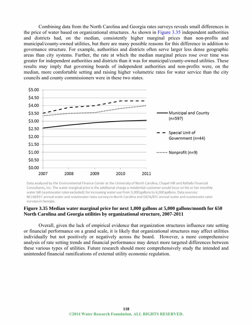
118
Combining data from the North Carolina and Georgia rates surveys reveals small differences in the price of water based on organizational structures. As shown in Figure 3.35 independent authorities and districts had, on the median, consistently higher marginal prices than non-profits and municipal/county-owned utilities, but there are many possible reasons for this difference in addition to governance structure. For example, authorities and districts often serve larger less dense geographic areas than city systems. Further, the rate at which the median marginal prices rose over time was greater for independent authorities and districts than it was for municipal/county-owned utilities. These results may imply that governing boards of independent authorities and non-profits were, on the median, more comfortable setting and raising higher volumetric rates for water service than the city councils and county commissioners were in these two states.
Figure 3.35 Median water marginal price for next 1,000 gallons at 5,000 gallons/month for 650 North Carolina and Georgia utilities by organizational structure, 2007-2011
Overall, given the lack of empirical evidence that organization structures influence rate setting or financial performance on a grand scale, it is likely that organizational structures may affect utilities individually but not positively or negatively across the board. However, a more comprehensive analysis of rate setting trends and financial performance may detect more targeted differences between these various types of utilities. Future research should more comprehensively study the intended and unintended financial ramifications of external utility economic regulation.
©2014 Water Research Foundation. ALL RIGHTS RESERVED.
119
References
Aqua. 2013. North Carolina Service Territory. [Online]. Available: <https://www.aquaamerica.com/our-states/north-carolina.aspx.> [cited April 15, 2013]
Beecher, J.A., P. Mann, Y. Hegazy, and J. Stanford. 1994. Revenue Effects of Water Conservation and Conservation Pricing: Issues and Practices. Columbus, Ohio: The National Regulatory Research Institute at Ohio State University.
Beecher, J. A. 1997. Water Utility Privatization and Regulation: Lessons from the Global Experiment. Water International, 22(1): 54-63.
Davey, M. 2013. Michigan Naming Fiscal Manager to Help Detroit. The New York Times, March 1, 2013. [Online]. Available: <http://www.nytimes.com/2013/03/02/us/michigan-appoints-emergency-manager-for-detroit.html?pagewanted=all&_r=0> [cited: May 9, 2013]
League of California Cities. 2007. Proposition 218 Implementation Guide. Sacramento, Calif.: League of California Cities.
Maine Revised Statutes. 1987. Title 35-A: Public Utilities Heading, Chapter 21: Organization, Powers, Service Territory Heading, § 2101. Organization of certain public utilities. [Online]. Available: < <http://www.mainelegislature.org/legis/statutes/35-A/title35-Asec2101.html> [cited May 9, 2013].
MNGWPD (Metropolitan North Georgia Water Planning District). 2009. Water Supply and Water Conservation Management Plan. Atlanta, Ga.: Metro Water District Board. [Online]. Available: <http://www.northgeorgiawater.com/plans/water-supply-and-water-conservation-management-plan> [cited April 15, 2013]
NC State Treasurer. 2013. Information on State and Local Government: Local Government Commission. [Online]. Available: <https://www.nctreasurer.com/slg/Pages/Local-Government-Commission.aspx> [cited April 15, 2013]
NCDENR (North Carolina Department of Environment and Natural Resources). 2013. 2008 Drought Bill Signed Into Law. [Online] Available: <http://www.ncwater.org/drought/> [cited April 15, 2013]
Seidenstat, P. 2003. Organizing Water and Wastewater Industries to Meet the Challenges of the 21st Century. Public Administration and Management: An Interactive Journal, 8(2): 69-99.
USEPA (United States Environmental Protection Agency). 2012. October 2012 data in Safe Drinking Water Information System Database. [Online]. Available: SDWISFED Drinking Water Data. <http://water.epa.gov/scitech/datait/databases/drink/sdwisfed/pivottables.cfm> [cited April 18, 2013]
WI PSC (Public Service Commission of Wisconsin). 2013. Information on the State’s water industry regulation. [Online]. Available: < http://psc.wi.gov/water/> [cited April 15, 2013]
FINANCIAL MANAGEMENT STRATEGIES Introduction
As with other business enterprises, many utilities striving for performance improvement adopt one or more integrated management theories, programs, or initiatives to guide their decision-making. A study of 15 different management initiatives carried out in 2004 concluded that creating an integrated management framework can lead to a greater chance of performance improvement than implementing discrete independent management practices (Integrated Management Systems Design Team 2004). Adopting a comprehensive approach to management can also help utilities rally around specific performance goals and create a shared institutional resolve to make difficult decisions. Management
©2014 Water Research Foundation. ALL RIGHTS RESERVED.
120
philosophies and systems can vary quite a bit; however, many of these business strategies include similar components relating to finance and revenue stability.
There are a number of integrated management theories utilized by water and wastewater utilities. These include Effective Utility Management (EUM), Lean, Six Sigma, and Total Quality Management (TQM). These techniques can be used alone or in concert to further utility financial and management goals. The Resource Guide to Effective Utility Management and Lean explains that EUM helps utilities to assess their strengths and weaknesses, prioritize their goals, and determine what outcomes the utility wants to achieve, while Lean and Six Sigma are business improvement approaches that focus on eliminating non-value added activity and help utilities to reach the desired outcomes.
Several utilities have effectively incorporated the concepts of EUM and Lean into their long-term strategies. This section of the report highlights the manner in which both of these management strategies address utility finances directly and highlights a case where the combination of the two had a direct financial impact. Key Points
Among other attributes, current management strategies in the industry, such as Effective Utility Management and LEAN, advance financial management.
The extent to which each and any management strategy has measurable impact on the financial condition and revenue resiliency of a utility could be the exclusive focus of an entire report.
Focus on Effective Utility Management as a Financial Management Driver
Since its inception, EUM has become more comprehensive, and is now serving as a framework
to help utility executives, governance boards, policy-makers, and regulators improve utility performance in a number of areas (AWWA 2008). The framework allows for planning, implementation, measuring, and monitoring performance enhancements against the Ten Attributes, which include:
Product Quality; Customer Satisfaction; Employee and Leadership Development; Operational Optimization; Financial Viability; Infrastructure Stability; Operational Resiliency; Community Sustainability; Water Resource Adequacy; and Stakeholder Understanding and Support.
Specifically focusing on Financial Viability, EUM cites well-managed utilities as:
“understanding the full life-cycle costs of the utility and establishing and maintaining an effective balance between long-term debt, asset value, operations and maintenance expenditures, and operating revenues.” Downward pressures on revenue due to falling sales and traditional pricing model has made maintaining this “balance” difficult for many utilities. The EUM Primer goes on to discuss the importance of establishing predictable rates to adequately cover costs, meet community expectations, provide for reserves, maintain support from bond rating agencies, and plan and invest for future needs. Metrics associated with financial viability include budget management effectiveness: debt ratio,
©2014 Water Research Foundation. ALL RIGHTS RESERVED.

121
revenue to expenditure ratio, O&M expenditures or capital expenditures, etc. While many of the tenets of Effective Utility Management have been widely recognized by utilities, a highly branded and endorsed framework may provide managers and boards facing difficult decisions with additional momentum to achieve financial resiliency. Focus on LEAN as a Financial Management Driver
As previously mentioned, LEAN refers to a set of principles and methods focused on the systematic elimination of non-value added activity. The principles and methods started with Toyota, in the manufacturing sector, and have since spread to diverse industries and sectors around the world. The idea is that people learn to see where inefficiency in resource use and deployment exists. This is often used in conjunction with Six Sigma, which is a statistical process that identifies process variation to improve overall quality.
Specifically relating to improving the financial state of utilities, LEAN offers several methods that help to ensure that resources are being used in the most effective way possible. For example, LEAN Events are two-five day periods where cross-functional teams of employees will analyze and improve a process. Six Sigma can also help to find and eliminate process variation, which can result in significant cost savings. Utilities adopt LEAN to:
Achieve better financial and operational results; Enhance customer service; Produce quality products and services; Optimize operational and administrative processes; Reduce risks and errors; and Improve staff morale and engage employees.
According to the “Resource Guide to Effective Utility Management and Lean, “One of the
most frequently cited benefits of LEAN is cost savings, which maps to the Financial Viability Attribute in the EUM system. Cost savings and cost avoidance are realized from process changes that allow utilities to avoid investing in costly new controls and increase machinery and process efficiency” (USEPA 2012). Utility Case Study City of Pompano Beach Utilities
The City of Pompano Beach Utilities Department (Department) serves approximately 80,000 customers in Pompano Beach, Florida. The Department has used both an EUM assessment and LEAN process-improvement tools to develop an action plan to move improvement activities forward. As a result, the Department has seen significant operational and management results, including increased water efficiency, improved customer satisfaction, and enhanced financial viability.
The Department started the improvement process with the help of a consulting group, which facilitated the EUM assessment. Based on the assessment findings, the highest priority areas for the Department were Product Quality, Financial Viability, Infrastructure Stability, Operational Optimization, and Employee and Leadership Development. The first task was then to create groups to focus on safety and job performance standards, and to systematically evaluate the processes in place and identify where failures might occur, so that process improvement could occur. The Department used a variety of LEAN and Six Sigma techniques to achieve the targets identified in the EUM assessment.
©2014 Water Research Foundation. ALL RIGHTS RESERVED.

122
One particular problem that the assessment found and LEAN helped to solve was the ICanWater Reuse Connection Program, which had seen low customer base penetration through 2011. By using the Six Sigma Define-Measure-Analyze-Improve-Control method, the Department was able to increase reuse connections from an average of 1.5 per month to more than 270 between October 2011 and April 2012, with an additional 770 planned by July 2013. This increase in reuse water addressed several of the attributes identified in the EUM assessment, including Financial Viability, by reducing pressure on drinking water supply and the need for expensive system upgrades (Oasis Reuse Water Utilities 2013).
The extent to which each and any management strategy has measurable impact on the financial condition and revenue resiliency of a utility could be the exclusive focus of an entire report. Most likely, more influential than the strategy itself is the manner in which it is applied. Suffice it to say an integrated management strategy, like Effective Utility Management and LEAN, drive integrated decision-making and prioritization which many studies have shown as a best practice in financial management. References AWWA (American Water Works Association). 2008. Effective Utility Management: A Primer for
Water and Wastewater Utilities. Denver, Colo.: AWWA. [Online]. Available: <http://www.watereum.org/resources/interactive-primer/> [cited May 9, 2013]
Integrated Management Systems Design Team. 2004. Continual Improvement in Utility Management: A Framework for Integration. Washington, D.C.: USEPA, Association of Metropolitan Sewerage Agencies, and Water Environment Federation. [Online]. Available: <http://www.peercenter.net/ewebeditpro/items/O73F3799.pdf> [cited May 9, 2013]
Oasis Water Reuse Utilities. 2013. I Can Water. Pompano Beach City, Fla.: Oasis Reuse Water Utilities. [Online]. Available: <http://www.icanwater.com/ > [cited May 9, 2012]
USEPA (United States Environmental Protection Agency). 2012. Resource Guide to Effective Utility Management and Lean: Improving Performance and Addressing Key Management Priorities at Water-Sector Utilities. Washington D.C.: USEPA. [Online]. Available: <http://www.epa.gov/lean/environment/pdf/eum-lean-guide.pdf> [cited May 9, 2013]
CREDIT RATING AGENCIES
Introduction
Water utilities considering, or in the process of, issuing debt through the capital markets often
decide to request a credit rating of that utility’s debt from one or more rating agencies, Standard & Poor’s, Moody’s, and Fitch Ratings. The rating is designed to provide information to prospective investors/lenders and influence utility access to, and the cost of, borrowing money. Fundamentally, each credit rating agency assesses the ability and willingness of an entity to repay impending debt issuance on-time and in-full, given the entity’s financial and operating circumstances. However, each credit agency focuses on slightly different qualitative and quantitative indicators to evaluate a utility’s credit strength.
In addition to individual utility ratings, rating agencies produce periodic sector reports and analyses that provide a wealth of general industry financial condition and trend information (summarized in Table 3.1). Individual utility reports, assessments, and special reports serve as an external third party reflection of the financial position of individual utilities and the industry as a whole. For many utilities, these external assessments also serve as important financial drivers and benchmarks behind internal financial policies and rate decisions.
©2014 Water Research Foundation. ALL RIGHTS RESERVED.
123
Key Points
Credit rating agencies weigh a myriad of qualitative and quantitative considerations when determining credit ratings; there is no pre-set formula for a good rating.
Ultimately, credit rating agencies are looking for flexibility, capacity, and predictability. Although the individual and summary reports from credit rating agencies provide a reflection
of the financial condition of the water industry, the processes engaged by credit rating agencies are also driving the financial priorities in the industry.
Traditionally, credit rating agencies view water demand as revenue, although there is some movement to recognize long-term, cost-effective conservation and efficiency efforts. The industry is challenged to account for “triple-bottom line” strategies due to scope and accounting limitations.
Reflection of Financial Position of Individual Water Utilities and the Industry as a Whole In general, credit rating agencies collect data on and evaluate the credit worthiness of the
country’s largest utilities because these utilities are primarily the entities issuing debt. At varying degrees of frequency, each credit rating agency releases their rating criteria – a summary of the multitude of qualitative and quantitative factors each agency considers when assigning a certain rating to an entity (summarized in Table 3.4).
©2014 Water Research Foundation. ALL RIGHTS RESERVED.

124
Table 3.4 Summary of Credit Rating Agency Guidance
Agency Rating criteria
Recent assessments and special reports
Ratings system
Number of Water and Wastewater Utilities Rated
Fitch Ratings
US Water and Sewer Revenue Bond Criteria (7/13)
2013 Water and Sewer Medians (12/5/12) 2013 Outlook: Water and Sewer Sector (12/5/12)
AAA AA (avg) A+, A BBB +,-
Approximately 400
Standard & Poor’s
Standard & Poor’s Public Finance Criteria (2008)
Sector Review: Funding Long-Term Needs Remains The Biggest Risk For U.S. Municipal Water And Sewer Utilities (1/31/12) How U.S. Municipal Water And Sewer Bond Ratings Correlate With Some Key Measures Of Issuers‘ Credit Quality (9/26/2011)
AAA AA A+/(median)- BBB +,-
Approximately 1,300
Moody’s Research and Ratings
Analytical Framework For Water And Sewer System Ratings (8/1999)
UK Water Sector Outlook 2011 Industry Outlook (10/2011)
Aaa Aa A Bb 1,2,3
Approximately 800
Other Players
The credit rating agencies are not the only entities collecting and evaluating the financial
performance and trends of the industry. Prudent public lenders, like the United States Department of Agriculture and state government loan programs, including the Environmental Protection Agency/State Revolving Loan Funds, as well as private lenders are evaluating the financial viability of the agencies they fund. In many cases, public sector and private capital lenders incorporate hard financial targets in loan agreements, while in other cases lenders monitor performance less formally. In addition, regulators such as public service and utility commissions evaluate and regulate the financial performance of the utilities in their state.
There are also a host of research, professional, and technical assistance organizations that promote the measurement and monitoring of financial performance and management strategies for the betterment of the industry. The financial metrics used and propagated by each of these organizations have significant overlap. The list below summarizes an example of a “Best Practice” advocated by one key organization, the Government Finance Officers Association (GFOA), for determining appropriate levels of working capital in enterprise funds. Many of the following “considerations” coincide with the metrics used by rating agencies.
©2014 Water Research Foundation. ALL RIGHTS RESERVED.

125
GFOA’s Primary considerations when customizing a working capital target for public enterprise funds
Support from general government Transfers out Cash cycles (i.e. peaks and valleys in in-flow) Customer concentration Demand for services Control over rates and revenue Asset age and condition Volatility of expenses Control over expenses Management plan for working capital Separate targets for operating and capital needs Debt position
No Formulas, Just Considerations
Much as the GFOA’s considerations in the list above include a mix of objective and subjective
indicators, the ratings agencies each use a number of quantitative and qualitative financial health metrics to prepare a utility’s financial profile and associated bond rating. As part of the project, specific ratings of utilities were studied, particularly for those utilities serving as partners on the project, as well as recent general guidance and criteria documents, to summarize the credit raters’ perspectives on revenue resilience. The finding: there is not a single pre-set formula for solid financial footing and a high credit rating. In fact, some of the metrics are in direct conflict with one another. For example, an excerpt of Standard & Poor’s ratings (summarized in Figure 3.36) highlight the importance that rating agency places on a history of rate increases, while at the same time recognizing the need for competitive and affordable rates.
©2014 Water Research Foundation. ALL RIGHTS RESERVED.

126
Periodically, Fitch Rating’s releases a report on “Water and Sewer Revenue Bond Rating Criteria” the explains in detail each criterion used by the agency to evaluate a utility’s credit worthiness, as well as provides an evaluation of stronger, mid-range, and weaker financial profiles. Although Fitch Ratings take into account many more quantitative metrics, they have also identified a list of “key” metrics summarized in the following table (Table 3.5).
Table 3.5
Fitch Rating’s Key Financial Ratios (Scott et al. 2013) Metric Definition Significance
Total outstanding long-term debt per customer
Total amount of utility long-term debt divided by the total number of utility customers (for a combined utility, the aggregate number of water and wastewater accounts are used)
Indicates the existing debt burden attributable to ratepayers (principal only)
Total outstanding long-term debt per capita
Total amount of utility long-term debt divided by total population served by the utility
Indicates the existing debt burden attributable to each person served by the utility (principal only)
Projected debt per customer
Total projected outstanding system debt (existing debt less scheduled amortization plus planned issuances) divided by total outstanding projected customers for five years from the date of the rating
Indicates the total debt burden to ratepayers five years from the date of the rating (principal only)
Projected debt per capita Total projected outstanding system debt (existing debt less scheduled amortization plus planned issuances) divided by total projected population served by utility (population is inflated based on anticipated growth)
Indicates the total debt burden to each person served by the utility five years from the date of the rating (principal only)
Three-year historical average senior lien annual debt service (ADS) coverage
Most recent three-year historical average of annual revenues available for debt service coverage divided by respective senior lien debt service for the year
Indicates the financial margin to meet current senior lien ADS with current revenues available for debt service
Three-year historical average all-in ADS coverage
Most recent three-year historical average of annual revenues available for debt service divided by respective total debt service for the year
Indicates historical trend in total ADS coverage
(continued)
©2014 Water Research Foundation. ALL RIGHTS RESERVED.

127
Table 3.5 (Continued)
Metric Definition Significance All-in ADS coverage Current-year revenues available
for debt service divided by current-year total debt service
Indicates the financial margin to meet current total ADS with current revenues available for debt service
Minimum projected all-in ADS coverage
Minimum debt service coverage projected typically over the ensuing five-year period, based on revenues available for debt service in any given fiscal year, divided by the respective total debt service amount for that fiscal year
Indicates the financial margin during the year in which future total ADS coverage is projected to be the lowest
Days cash on hand Current unrestricted cash and investments plus any restricted cash and investments (if available for general system purposes), divided by operating expenditures minus depreciation, divided by 365
Indicates financial flexibility to pay near-term obligations
Days of working capital Current unrestricted assets plus any restricted cash and investments (if available for general system purposes), minus current liabilities payable from unrestricted assets, divided by operating expenditures minus depreciation, divided by 365
Indicates financial flexibility to pay near-term obligations
Free cash as a % of depreciation
Current surplus revenues after payment of operating expenses, debt service, and operating transfers out divided by current year depreciation
Indicates annual financial capacity to maintain facilities at current level of service from existing cash flows
Standard & Poor’s and Moody’s have similar lists of metrics they purport as critical to their
credit ratings, but each credit rating agency may weigh these factors slightly different resulting in rating level variance between the three. In addition to measuring a utility’s ability to meet its operating and debt expenses under normal and slightly altered conditions, rating agencies stress the importance of metrics that gauge economic capacity (household/per capita effective buying income as a percentage of U.S. level), revenue diversity (top ten customers as a percentage of total operating revenues), and off-balance sheet fixed financial obligations.
In their criteria documents, both S&P and Fitch Ratings stress that quantitative metrics and ratios cannot completely portray the financial condition of a utility (Standard & Poor’s 2007; Scott et al. 2013). Economic, management, structural, and other qualitative factors may be given equal, if not more weight when assessing an entity’s ability and will to meet its financial obligations. Fitch Ratings has coined the phrase “10 C’s” to alliterate its portfolio of considerations including: community characteristics, customer growth and concentration, capacity, compliance with environmental laws and
©2014 Water Research Foundation. ALL RIGHTS RESERVED.

128
regulations, capital demands and debt policies, covenants, charges and rate affordability, coverage and financial performance, cash and balance sheet considerations, and crew.
Figure 3.36 Key credit rating considerations of S&P for 18 drinking water utilities from 2010-2012
The word cloud above identifies analyses trends among a group of Standard & Poor’s ratings for 18 of our utility partners prepared between 2010 and 2012. (The larger a word or phrase, the more often it was cited.) In most cases, we’ve stripped the considerations of non-quantified adjectives like strong, steady, and aggressive to draw attention to common themes and considerations. (It’s important to note that in the analysis above each utility received an AA or AAA rating from S&P.) Some prominent rating concerns like service area (Is the customer base large and diverse, or small and concentrated?) and customer wealth are outside the control of utility officials. Credit raters also consider income levels, housing values, employment patterns, and population growth. However, many of the recurring concerns (such as financial coverage and rate increase history) fall under the direct influence of utility management. Furthermore, the credit rating agencies are analyzing a utility’s preparation and response to the factors outside of its control, with a focus on flexibility, capacity, and predictability. Financial Focus on Flexibility, Capacity, and Predictability
In addition to hitting different variations of key debt service coverage ratios, Fitch Ratings and Standard and Poor’s place high value on utilities whose “day-to-day operations are relatively free from political interference” (Scott et al. 2013) and utilities that display “rate flexibility”; that is, they are willing and able to increase rates as necessary to cover costs (Dyson 2011). In a 2012 report, Moody’s discusses this “willingness” as a combination between the flexibility and capacity of organizations to manage rates and costs (Medina et al. 2012). In general, credit rating agencies define a resilient utility as one that has revenue and resource flexibility, capacity, and predictability. Of course, these attributes are also important when assessing costs as well. The following excerpts from credit rating summaries
©2014 Water Research Foundation. ALL RIGHTS RESERVED.
129
highlight areas where flexibility, capacity, and predictability were addressed in general guidance or specific summaries from credit rating agencies.
Flexibility
As monopolies, governance structure and pricing strategy largely govern the flexibility of a utility. Credit rating agencies are looking for evidence of a utility’s will to utilize this flexibility.
To Increase Rates. Credit rating agencies are assessing whether or not political leaders and
utility officials have, and will, raise rates.
Alameda, CA. “The district has historically raised rates annually, which has led to increased operating revenue over time and has offset some of the effects of conservation in recent years.” (Hannay and Dyson 2012). AAA/Stable
Austin, TX. “City officials have demonstrated their willingness to raise rates…” (Chapman and Murphy 2011). AA/Stable
Metropolitan Water District, CA. “On April 10, 2012, the district's board voted to increase rates by an average of 5.0% in each of the next two calendar years, 2013 and 2014. The 2013 increase is less than what district staff had proposed (7.5%) but more than the district's most vocal critics wanted (0-3%). This 5% compromise position, which keeps the cost of "wholesale supplies as low as possible" according to the district's board chairman, raises the specter that the district's previous above-average willingness to raise rates when necessary may be weakening in the face of increasingly vocal criticism. While we recognize the rhetorical appeal and inherent vagueness of keeping rates "as low as possible," in the long-run such rates will not maintain the district's long-term credit quality at a level consistent with its current rating.” (Moody’s Investors Service 2012) Aa1
Fort Worth, TX. “The downgrade reflects weak financial performance stemming from the city's lack of willingness to raise rates in the current fiscal year to offset reduced water sales. Given this unwillingness, Fitch is concerned that the city may be reluctant to implement the magnitude of rate increases needed to regain historical margins.” (Seebach and Wenck 2013) AA
To Absorb Temporary Financial Shocks. Reserves are commonly cited as a financial positive
because they allow a utility to absorb temporary financial shocks, such as those caused by the implementation of watering restrictions in response to an unexpected water shortage. The number of “days-of-cash” on hand that a utility has indicates how long it could operate with absolutely no new revenue. This report discusses the use of reserve funds as a strategy for revenue resiliency in great detail. Despite placing high value on the existence of these reserves, Standard & Poor’s cautions against the reliance on reserves, as they provide a limited amount of additional security and are sometimes used as a political “backdoor” to making unsustainable financial decisions (Chapman 2012d).
Alameda, CA. “The district’s liquidity position is strong, in our view (Unrestricted cash
and investments represent 610 days of operating expenses)” (Hannay and Dyson 2012). AAA/Stable
Daphne, AL .“Although the board may draw down unrestricted cash and investments from 458 days of operational expenses, one of the board’s financial principles is to
©2014 Water Research Foundation. ALL RIGHTS RESERVED.

130
maintain unrestricted cash equal to at least 120 days’ expenditures (Sagen and Waite 2012).” AA-/Stable
Glendale, CA- “The negative outlook reflects our view that if unrestricted cash remains near $0 during the next two years as debt service and debt levels increase, we will likely lower the rating. In the nearer term, we believe the currently high debt service coverage (3.5x) and the ability of the water fund to borrow from the electric fund provide the water system some financial flexibility (Chapman and Hannay 2011).” AA/Negative
From Environmental Regulation. Credit rating summaries typically view and discuss
regulation as a driver of capital costs outside utility control that can compromise a utility’s ability to increase rates and cover costs. “External regulations, government intervention, or scrutiny over affordability can limit an issuer’s ability to direct their own operations” (Medina et al. 2012)
Jackson, MS. “The sewer system is under a state order from the Mississippi
Commission on Environmental Quality (MCEQ) to address sewer overflow and sludge violations. …. Although consent decree requirements will likely allow the city multiple years to address identified sewer issues, the capital costs are expected to be large and could total as much as $600 million. The city's ability to handle this amount of capital requirements given the lack of rate-raising history and financial / capital planning is reflected in the negative outlook. ….We will continue to monitor the outcome of the consent decree and management's ability to plan for and manage the expectedly large capital requirements.” (Moody’s Investors Service 2011) Aa1
Atlanta, GA. “Although the city council’s resolution reiterates its commitment to comply with consent orders and current rate increases, in our opinion, the internal audit requirement together with management’s efforts to obtain an extension on meeting consent order milestones based on affordability guidelines signals increased rate sensitivity.” (Breeding and Sugden-Castillo 2011) A/Stable
Capacity
To Increase Rates. Credit rating agencies are assessing how “high” a utilities rates are by comparing its rates are to those in surrounding areas and similar utilities. Low rates, when considered in the context of service area income levels, indicate a capacity to increase rates. If a utility is deemed to have high rates, affordability pressures may arise that could significantly decrease a utility’s capacity to increase rates. Credit ratings take into consideration capital improvement plans (CIPs) and approaches large CIPs with caution – weighed very heavily against the capacity of the utility to increase rates.
Austin, TX. “Despite rate increases, the $71 residential bill for 8,000 gallons of combined service is especially competitive because of the water supply agreements already in place (Chapman and Murphy 2011).” AA/Stable
Raleigh, NC. “Management has demonstrated a willingness to adjust rates….Despite annual increases, the system’s rates are still affordable relative to service area wealth levels. We expect management to continue to adjust rates as needed (Pezzimenti and Costa 2012).” AAA/Stable
Fort Worth, TX. “The combined water and sewer monthly bill of $62.46 (assuming usage of 7,500 gallons per month for both water and sewer) equals a moderate 1.5% of median household income, providing the system sufficient rate flexibility.” (Seebach and Wenck 2013) AA
©2014 Water Research Foundation. ALL RIGHTS RESERVED.

131
To Meet Demand. Credit rating agencies are also viewing capital and resource plans of utilities to evaluate their capacity to meet demand. Demand equals revenue. In general, if a utility does not have the capacity to meet demand, it means lost revenue. The following excerpts provide insight into direct considerations of this relationship.
Metropolitan Water District, CA. In dealing with short-term water shortages, like
drought, Standard & Poor’s praised the Metropolitan Water District of Southern California for engaging effective drought policies to match demand to supply. “MWD implemented a 10% reduction in water available to customers in 2009 due to drought and reaffirmed it in April 2010. –However, they built up storage capacity to fill up when conditions are wet so that they can sell water during drought (Dyson and Hannay 2011).” AAA/Stable
Daphne, AL. “The system’s diverse customer base is still growing, albeit at, what we consider, a more-moderate pace; system treatment capacity adequately meets current demands.” (Sagen and Waite 2012) AA-/Stable
Atlanta, GA. According to the Atlanta Journal Constitution (AJC), local governments in metro area Atlanta received a report from the credit agency Fitch Ratings, warning that their credit scores may be downgraded depending on the outcome of a federal lawsuit over access to drinking water from Lake Lanier. According to AJC, Fitch warned that water will “continue to be a primary rating driver,” given “the devastating effect any material reduction would have on the region” (Joyner 2011). In late spring 2012, the 11th Circuit Court of Appeals upheld Atlanta’s right to draw its drinking water supply from Lake Lanier, thus forestalling its water and credit woes for the near future.
Predictability
In addition, credit rating agencies take into account decision-making and financial arrangements between a utility and its governing body. Obviously, the governance structure of a utility and established contracts fall out of the exclusive control of utility management, but the credit rating agencies are also assessing the process and predictability of the arrangement. For example, S&P does not necessarily view a transfer from a public enterprise fund to the general fund of the governing body as a negative factor, as long as the transfer policy is “well-researched, flexible, consistent, and well-communicated (Standard & Poor’s 2007).” How a utility reacts, or better yet, anticipates its operating environment largely factors into its rating. Water Demand
Historically, credit rating agencies cite aggressive conservation programs as weaknesses
because they have a direct and immediate impact on operating revenue. In 2011, Standard & Poor’s noted that the City of Austin, Texas’ financial metrics would have “looked stronger, if it weren’t for the City’s aggressive water conservation and resource management program (Chapman and Murphy 2011)”. Meanwhile, Fitch Ratings recognized those utilities that “were able to meet rising consumptive demand without significant usage restrictions (Scott et al. 2011).” When assessing whether or not a drought will impact a utility’s credit rating, Fitch Ratings identified the following factors (summarized in Table 3.6). This Water Research Foundation report contains discussion and financial strategies around many of the factors that are under management’s control.
©2014 Water Research Foundation. ALL RIGHTS RESERVED.

132
Table 3.6 Drought-time credit considerations by Fitch Ratings and assessment of utility control
Fitch Ratings’ factors (Scott et. al 2011) Is this factor under management’s control
Current drought stage No Current and anticipated drought restrictions Somewhat Level of precipitation needed to end drought restrictions compared to historical precipitation amounts
Somewhat
Current actions to avoid water shortage and availability of alternative supplies
Somewhat
Current and anticipated effect of drought on demand, revenues, and expenses
Somewhat
Current actions to mitigate the drought’s effect on utility financial performance
Yes
Degree of revenue certainty from base charges relative to budgeted revenues
Yes
Usage assumption used in current budget Yes Anticipated actions to ensure financial health should drought continue
Yes
Lasting effects of drought on supply costs, customer demand, etc.
No
In coping with present and future water shortages, credit rating agencies seem to be beginning
to recognize that while conservation efforts can impact revenues and financial risk profiles (fixed-charge coverage ratio is negatively impacted by conservation and wet weather) in the short-term, such efforts are necessary to deal with long-term risks associated with supply shortages and high costs of capital (Chapman 2012b; Leurig 2012). In their guidance reports for utilities, there is consensus that financially prudent utilities will account for the long-term benefits of conservation and long-range planning, including deferred costs of capital via demand reduction, incremental decreases in operating costs (such as electricity for pumping and water treatment chemicals), and ability to manage risks associated with seasonal water use variability (Chapman 2012d; Scott et al. 2013). Pricing and Rate Structures
Drought and seasonal variability are closely related to a utility’s revenue resiliency because of
pricing and rate structures. In 2012, Standard & Poor’s recognized that although the Alameda Water District’s operating revenue had experienced the “effect of conservation in recent years,” some of these effects were mitigated by annual rate increases and therefore retained their AAA/Stable rating by the agency (Hannay and Dyson 2012). And while the rating agency rebuked the City of Austin, Texas for its aggressive water conservation and resource management programs, they praised the utility for its plans to update its business model by adding a fixed revenue stability fee (Chapman and Murphy 2011). Fitch Ratings views favorably a utility whose fixed portion (base charge) of the water and wastewater bill makes up greater than 30% of the total bill (Scott et al. 2013), although it is not currently reported on its median report.
This later point alludes to the regard for fixed revenue over variable revenue by credit rating agencies and the lending institutions on whose behalf they work. Revenue that is dependent on discretionary water use can compromise a utility’s financial health when faced with drought
©2014 Water Research Foundation. ALL RIGHTS RESERVED.

133
restrictions in the short-term and its credit rating soon thereafter (Leurig 2012). However, the credit rating agencies, and in fact many utilities themselves, stop short of discussing the degree of vulnerability posed by the design of certain rate structures.
The Cart Leading the Horse: The Driving Power of Credit Rating Financial Metrics
Up until this point, credit rating agencies and the metrics they use have been discussed as a
reflection of an individual or group of utility’s financial performance. However, there is a management adage that suggests “what gets measured, gets done.” In 1954, Peter Drucker published a book entitled “The Practice of Management” that suggests that if people are accountable to a certain metric, they will forsake other non-measured efforts to meet or succeed the measured effort. Given that credit rating agencies are probably the most influential financial surveyors of the industry, the metrics they use, at least in a small part, set the bar against which utilities develop their own financial policies.
But credit rating agencies guide the financial policies by more than just defining the metrics. In fact, certain ratings have become the overarching goal of the financial policies set by utilities. For example, Charlotte-Mecklenburg Utilities Department’s financial policy stresses the importance of maintaining a AAA bond rating from the three credit rating agencies, according to an interview with CMUD director, Barry Gullet (Gullet 2012). The utility set its financial performance goals by benchmarking against other AAA rated utilities and consulting with financial advisors.
Charlotte-Mecklenburg Utilities is not alone. Others in our utility cohort had similar guidance set forth in their financial policies as summarized below:
“Denver Water’s debt guidelines state the organization’s desire to maintain the
standalone revenue bond rating at a level of AA or better.” (Denver Water 2012) Objective A: Maintain AAA 7-year financial goals and meet appropriated designated
fund level goals.” (Mesa Waterer 2011) Credit rating is one of the performance measures tracked by the Office of the General
Manager at the Metropolitan Water District of Southern California. The intent of the measurement is to “enable Metropolitan to access capital markets at the lowest borrowing cost.” The target is set at AA, Aa2 or better. (Metropolitan Water District of Southern California 2010)
“Maintain WaterOne’s current Bond ratings for senior debt of AAA from S&P and Aaa from Moody’s.” (Water District No. 1 of Johnson County 2012)
The [Clayton County Water] Authority’s primary objectives [of its debt policies] are to minimize debt service and issuance costs; maintain access to cost-effective borrowing; achieve the highest practical credit rating; ensure full and timely repayment of debt; maintain full and complete financial disclosure and reporting; and ensure compliance with applicable state and federal laws.” (Clayton County Water Authority 2011)
Clayton County Water Authority’s open-ended objective of achieving the highest practical
credit rating indicates that there are some costs associated with achieving the highest credit rating. Future analysis should look into just what these costs and benefits are. According to the Director of Charlotte-Mecklenburg Utilities, maintaining AAA bond rating means more to his utility than a lower interest rate, it ensures that the utility (and City) have access to the market when they need it, so that both can maintain liquidity (Gullet 2012).
For many utilities, a lower interest rate can lead to substantial cost savings on bond repayments. Figure 3.37 shows the differences in the interest rates for 20th year maturity by credit rating grade.
©2014 Water Research Foundation. ALL RIGHTS RESERVED.

134
Interest rates for credit ratings Aa, A, and Baa remain fairly widespread over time; however, prior to 2008 the spreads were generally less than 0.3% and are now consistently over 0.5%.
Figure 3. 37 Municipal market interest rates for 20th year maturity by credit rating (WM Financial Strategies 2013)
Table 3.7 shows the differences bond debt for an Aa rated utility, and a Baa rated utility for a $40,000,000 bond for interest rates in 2009 and 2013. After one year at the 2009 interest rate, there is a one million dollar difference in interest owed. At the 2013 rate however, this difference drops to $460,000 (WM Financial 2013). Thus, it is clear that a utility’s credit rating can have a significant financial impact, but how do those financial benefits compare to the costs of maintaining very high debt service coverage ratios and reserves that need to go largely “untouched?” Future research is needed to weigh the true costs and benefits of certain credit ratings.
Table 3.7 Cost savings from interest rate differences due to credit rating
Principal Credit Rating
Interest Rate (2009)1
Interest Rate (2013)1
Principal + Interest After 1 year (at 2009 rate)
Principal + Interest After 1 year (at 2013 rate)
$40,000,000 AA 0.049 0.0275 $41,960,000 $41,100,000 $40,000,000 BAA 0.074 0.039 $42,960,000 $41,560,000
Cost Savings in 1 year: $1,000,000 $460,000 1Interest Rates calculated from Figure 3.3
©2014 Water Research Foundation. ALL RIGHTS RESERVED.
135
Conclusion and Gap Analysis If indeed the credit rating agencies are steering the financial decisions of some of nation’s
largest utilities, where are they taking the industry? Are there unintended consequences of the quantitative and qualitative guidance explicitly and inexplicitly communicated through individual utility credit ratings? Scope and accounting limitations
Credit rating agencies are ultimately beholden to the lenders, not to water customers, in their
assessment of utility financial health. And lenders are concerned about the financial health for the tenure of the debt: 20, 10, 5 years or less. As such, credit rating agencies are short-sighted in their ability to integrate innovations in water utility infrastructure into their ratings systems, specifically those designed to address the “triple bottom line.” For example, at this point, the key agencies have not devised a methodology for assessing a utility’s green infrastructure or low impact development assets, such as cisterns. In this paradox of innovation and proven reliability between the utilities and the ratings agencies, up to this point, utilities have a limited ability to accurately convey information about the financial and environmental advantages of investments into innovative practices or to demonstrate the value of such practices relative to comparable utilities (Augustyn, Leurig, and Odefey 2012). A growing number of cities are meeting regulatory standards and cutting costs by installing green infrastructure. Yet some organizations such as American Rivers argue that there is a lack of credible valuation or accounting for natural infrastructure or other ecosystems services (American Rivers et al. 2012).
Additionally, ratings agencies, industry groups, and policy makers use four main financial metrics to identify investment and physical asset replacement: operating ratio (Bernstein 1993), age of plant (Hessenthaler, Masterson, and Quiroga 2008), fixed asset turnover (Bhattacharya 1995), and infrastructure condition (Garvin 2003). However, the financial statements and accounting behind these metrics are founded on recording assets at their historic or book value – the value, in nominal dollars, at which assets were purchased. This convention, combined with the common approach to depreciation of assets (straight-line depreciation) leads to some distortions between the economic value of the assets and the value reported on the annual financial statements (Ratcliffe and Munter 1981). Another impact of this accounting system is that utility accounting systems remain unable to attribute value to natural assets that provide water storage, filtration, and delivery. This makes it difficult to include such assets on a utility’s balance sheet, or to finance the acquisition or development of these assets on the bond market (Hughes 2009).
As an example, over the next 13 years, Seattle Public Utilities estimates it will spend about $500 million on capital construction projects including retrofits, green infrastructure, and large underground storage tanks. Through these “green investments”, the utility estimates it will save approximately $375 million in future operating and maintenance costs over 13 years (SPU 2012). How the city will account for the value and depreciation of these assets, which are decentralized in nature and may not be owned by the city (i.e. green roofs, parking lot bio swales), continues to vex utility financial staff. Credit ratings agencies’ general outlook on innovations in green infrastructure and technology adoption is that utilities’ financial risk is reduced only at the point where the innovation is proven reliable and effective at meeting regulatory and service requirements at a utility-wide scale (Chapman 2012c). The sector has yet to develop a uniform methodology to account for unconventional water quality and conservation infrastructure in their asset portfolios. Nonetheless, they currently serve as good resource and driving force behind the financial performance of many of the nation’s water utilities.
©2014 Water Research Foundation. ALL RIGHTS RESERVED.

136
References American Rivers, Ceres and The Johnson Foundation. 2012. Charting New Waters: Financing
Sustainable Water Infrastructure. Racine, Wis.: The Johnson Foundation at Wingspread. Augustyn, F., S. Leurig, and J. Odefey. 2012. Restoring Flows : Financing the Next Generation of
Water Systems. Washington, D.C.: Ceres and American Rivers. Bernstein, L.A. 1993. Financial Statement Analysis : Theory, Application, and Interpretation. 6th ed.
Boston, Mass.: Irwin/McGraw-Hill. Bhattacharya, H. 1995. Total Management by Ratios: An Integrated Approach. New Dehli, India: Sage
Publications. Chapman, T. 2012a. Dry as a Bone: The Drought Spurs Municipally-Owned Utilities to Rethink Their
Long-Term Plans and Funding. Dallas, Tex.: Standard & Poor's Ratings Services. Chapman, T. 2012b. From Droughts to Conservation: Water Can Have Big Effects on U.S. Municipal
Utility Credit Quality. Standard & Poor's Credit Week, March 7. Chapman, Theodore. 2012c. Interview by Christine Boyle. Telephone. Chapel Hill, N.C., September
5th, 2012. Chapman, T. 2012d. U.S. Municipal Water and Sewer Utilities: Funding Long-Term Needs Remains
Their Biggest Risk. Standard & Poor's Credit Week, March 7. Clayton County Water Authority. Clayton County Water Authority. 2011. Authority Law and Policy
Manual. Morrow, Ga.: Clayton County Water Authority. Denver Water. 2012. Denver Water 2012 Budget: Summary of Financial Policies. Denver, Colo.:
Denver Water. [Online]. Available: <http://www.denverwater.org/docs/assets/64063362-DF55-A26C-B6A2EE661B764088/BudgetBook2012.pdf> [cited May 1, 2013]
Drucker, P.F. 1954. The Practice of Management. New York, N.Y.: Harper & Row. Dyson, P. 2011. Global Credit Portal: Metropolitan Water District of Southern California;
Water/Sewer. San Francisco, Calif.: Standard & Poor’s. Garvin, M.J. 2003. Strategic Characterization of Water System Infrastructure and Management. New
York, N.Y.: Columbia University Press. Gullet, Barry. 2012. Interview by author. Telephone. June 15, 2012. Hessenthaler, S.D., K. Masterson and G. Quiroga. 2008. 2008 Median Ratios for Water and Sewer
Revenue Bonds. New York, N.Y.: Retail Systems. Hughes, S. 2009. Beyond the Operating Ratio: Using Financial Statement Analysis to Assess Fixed
Capital Investments. Chapel Hill, N.C.: University of North Carolina. Joyner, C. 2011. Water Wars Threaten Credit of Metro Government. The Atlanta Journal-Constitution,
June 3. [Online] Available: <http://www.ajc.com/news/news/local-govt-politics/water-wars-threaten-credit-of-metro-governments/nQt6t/> [cited on May 1, 2013].
Leurig, S. 2012. Water Ripples: Expanding Risks for U.S. Water Providers. Boston, Mass.: Ceres. Mesa Water. 2011. Mesa Consolidated Water District Strategic Plan. Costa Mesa, Calif.: Mesa Water
District (Mesa Water). Medina, J., J. Aingorn, K. Krummenacker, M. Matesanz, D. Aschenbach, C. M. Hu and J. Hempstead.
2012. US Public Infrastructure: Slow Economic Recovery Tests Willingness to Manage Rates and Costs, October 23. New York, N.Y.: Moody’s Investors Service.
Metropolitan Water District of Southern California. 2010. Biennial Budget for Fiscal Years 2011/12 and 2012/13. Los Angeles, Calif.: Metropolitan Water District of Southern California.
NC Urban Water Consortium. 2012. Analysis conducted on utility residential billing records for NC Urban Water Consortium. Chapel Hill, N.C.: Environmental Finance Center.
Ratcliffe, T. and Munter, P. 1981. Complete Handbook of Inflation Accounting. Englewood Cliffs, N.J.: Prentice-Hall, Inc.
©2014 Water Research Foundation. ALL RIGHTS RESERVED.

137
Scott, D., G. Gutierrez, J. Seebach, and T. Wenck. 2011. Fitch Ratings Special Report: Texas-Sized Drought for the Lone Star State. New York, N.Y.: Fitch Ratings.
Scott, D., K. Masterson, A. Booker, and A. DeStefano. 2013. US Water and Sewer Revenue Bond Rating Criteria. New York, N.Y.: Fitch Ratings.
SPU (Seattle Public Utilities). 2011. Adopted Budget. Seattle, Wash.: SPU. [Online]. Available: <http://www.seattle.gov/financedepartment/11adoptedbudget/documents/spufromutilitiesandtransportation.pdf> [cited on May 21, 2013]
Standard & Poor’s. 2007. Public Finance Criteria: Financial Management Assessment. New York, N.Y.: McGraw-Hill.
Standard & Poor’s Credit Research. 2012. Dry As a Bone: The Drought Spurs Municipally-Owned Utilities to Rethink Their Long-Term Plans and Funding. Cited in Leurig, S. 2012. Water Ripples: Expanding Risks for U.S. Water Providers. A Ceres Report. [Online]. Available: <http://www.ceres.org/resources/reports/water-ripples-expanding-risks-for-u.s.-water-providers/view.> [cited May 1, 2013]
Water District No. 1 of Johnson County. 2012. Budget 2012: Fiscal Policies & Procedures. Lenexa, Kan.: Water District No.1 of Johnson County.
WM Financial. 2013. Rates Over Time: Interest Rate Trends. [Online]. Available: <http://www.munibondadvisor.com/market.htm>. [cited May 1, 2013]
Credit Ratings Breeding, J. and J. Sugden-Castillo. July 2011. Atlanta, Georgia; Water/Sewer Rating for Standard &
Poor’s. Long Term Rating: A(SPUR)/Stable. Dallas, Tex: Standard & Poor’s. Chapman, T. and R. Hannay. July 2011. Glendale, California; Water/Sewer Rating for Standard &
Poor’s. Long Term Rating: AA(SPUR)/Negative. San Francisco, Calif.: Standard & Poor’s. Chapman, T. and P. Murphy. November 2011. Austin, Texas; Water/Sewer Rating for Standard &
Poor’s. Long Term Rating: AA/Stable. Dallas, Tex: Standard & Poor’s. Dyson, P. and R. Hannay. August 2011. Metropolitan Water District of Southern California Rating for
Standard & Poor’s. Long Term Rating: AAA/Stable. San Francisco, Calif.: Standard & Poor’s. Hannay, R. and P. Dyson. January 2012. Alameda County Water District Financing Authority,
California Alameda County Water District; Water/Sewer Rating for Standard & Poor’s. Long Term Rating: AAA/Stable. Unenhanced Rating: AAA(SPUR)/Stable. San Francisco, Calif.: Standard & Poor’s.
Moody’s Investors Service. February 2013. Moody’s assigns Aa1 rating to Metropolitan Water District of Southern California’s Water Revenue Refunding Bonds. New York, N.Y.: Moody’s Investor Services, Inc. [Online]. Available: <http://www.mwdh2o.com/mwdh2o/pages/finance/PDFs/Moody's_Report.pdf > [cited May 1, 2013]
Moody’s Investors Service. August 2011. Moody’s downgrades City of Jackson’s (MS) Water and Sewer Revenue Debt to Aa3 from Aa2; assigns Aa3 rating to series 2011A and 2011B Revenue Debt issuances; Outlook is Negative. New York, N.Y.: Moody’s Investors Services, Inc. [Online]. Available: <http://www.bondsonline.com/print/Todays_Market/Credit_Rating_News_.php?DA=view&RID=19087> [cited May 1, 2013]
Pezzimenti, J. and P. Costa. March 2012. Raleigh, North Carolina: Water/Sewer Rating for Standard & Poor’s. Long Term Rating: AAA/Stable. New York, N.Y.: Standard & Poor’s.
Sagen, S. and J. Waite. February 2012. Daphne Utilities Board, Alabama; Combined Utility Rating for Standard & Poor’s. Long Term Rating: AA-/Stable. Dallas, Tex: Standard & Poor’s.
©2014 Water Research Foundation. ALL RIGHTS RESERVED.

138
Seebach, J. and T. Wenck. April 2013. Fitch Ratings downgrades its rating on the following Fort Worth, Texas (the city) outstanding revenue bonds: --$530.7 million water and sewer system (the system) revenue bonds to 'AA' from 'AA+'. Austin, Tex: Standard & Poor’s.
©2014 Water Research Foundation. ALL RIGHTS RESERVED.

139
CHAPTER 4: STRATEGIES AND PRACTICES FOR REVENUE RESILIENCY
DEMAND PROJECTIONS
Introduction
The “new normal” for water utilities has been categorized as one of declining sales and
increasing costs. Research and anecdotes across the country cite a general trend of decreasing water usage from customers due to a combination of increased efficiency standards (Rockaway et al. 2011), utility conservation and efficiency programming, and higher water prices. Depending on a utility’s perspective and circumstances, declining sales can be an unwelcome obstacle to financial stability or a strategy to long-term financial sustainability, particularly when sales decreases come in the form of reduced peak demands. Many environmental advocates point out that reducing demand can be a strategy for alleviating the increasing costs faced by the industry (Hoffner 2008; Leurig 2012). Referred to as “avoided costs” (Beecher 1996) or “hidden reservoirs” (Hoffner 2008) avoiding or deferring direct and indirect costs of water and wastewater provision by reducing peak demand for water can lead to a significant deferral of investment. The California Urban Water Conservation Council uses avoided cost to evaluate the benefit (or cost) of potential conservation programs to underscore its theory that improved water-use efficiency can complement or substitute for investments in long-term water supplies and infrastructure (Chesnutt and Beecher 2004; Hunter et al. 2011; Bishop and Weber 1996).
While planned-for and expected decreases in demand can serve as an efficient and potentially financially advantageous alternative water source, rapid unexpected drops in service sales can lead to short term financial stress and a drop in financial performance as measured by traditional financial metrics, such as operating ratio and debt service coverage. Clearly, producing accurate sales projections that account for the decline in consumption is a major component in planning for financial resilience. How water resource planners integrate long-term water use trends can impact utilities’ financial health if expensive raw water requirements and new supply projects are needlessly pursued (DeOreo and Mayer 2012).
Water utilities have typically erred on the side of over-estimating customer demand for multiple reasons including:
(1) The risk to public health of over-projecting demand are much less than of under-projecting demand; (2) A historic trend of increasing demand, and (3) Assurance that the system will have capacity to support community development and growth that may or may not have been accurately forecast.
Although, the public health risks still remain if a utility under-predicts demand, financial
pressures are increasingly leading utilities to become more conservative with their sales projections. Additionally, over-predicting sales and investing in infrastructure to meet that demand can risk public health if a utility forsakes expansion over infrastructure repair and replacement (Table 4.1).
©2014 Water Research Foundation. ALL RIGHTS RESERVED.

140
Table 4.1 Financial repercussions of demand projections
Actual demand decreases Actual demand increases Projected decrease in demand
Balanced budget; delayed capital investment delayed
Revenue surplus; potential capacity constraint
Projected increase in demand
Revenue deficit; underutilized capacity
Balanced budget; utilized capital
Because of the financial risk associated with demand over-prediction, credit rating agencies
have just begun to negatively view utilities that over-predict their demand (Leurig 2012). Ultimately this could result in a utility that already has less revenue than it projected facing increased borrowing costs. In addition, negative public perception of inaccurate projections can impact a utility’s ability to recover revenue. When a utility has to drastically increase rates because it over-predicted demand and revenue, customers will likely feel “punished” for conserving. By accurately projecting demand, utilities can reduce the rate lag between “cost-occurrence and cost-recovery (Beecher and Chestnutt 2012).”
Industry guides present various methods for forecasting demand that require varying degrees of sophistication. As billing, metering, and computing technology improve, utilities have an increasing ability to understand the baseline demand of their customers and to model demand under varying circumstances. This section of the report will not cover the process of forecasting demand from a technical standpoint, but rather point out general practices and examples in demand forecasting that can help a utility stabilize revenue. Key Points
Just as grocery and other retail stores use customer loyalty cards to set prices, market, and plan inventory, water utilities have the opportunity to use customer-level information to drive rate setting, budgeting, capital planning, resource management, conservation programming, and program marketing.
In frequently updating demand projections, utilities are more likely to detect major adjustments in customer behavior, like seen in a “drought hangover” and congruently adjust plans.
Detailed, integrated, and updated demand forecasting can help water resource managers and finance officers make plans with more confidence and less financial risk.
Practices for Improving Revenue Projections Linked to Sales Customer-Level Analysis
Customer consumption information is typically the foundation of future sales projections. The simplest way for a utility to forecast future sales is from a baseline of aggregated service-area wide sales. For example, projecting system-wide sales will increase 2% per year. For many utilities, this aggregated method has provided acceptable results, however as customers become more diverse and sensitive to different usage drivers, aggregating all customers in demand projections becomes potentially much less accurate. Demand projections are greatly improved if a utility can establish a baseline of individual customer demand patterns or even segments of customers – through customer-level billing analysis (Boyle et al. 2011) or, even better, by customer end uses (Levin et al. 2006).
For example, between fiscal years 2007 and 2008, the Fayetteville Public Works Commission saw a nine percent increase in average household water use over their entire residential customer base
©2014 Water Research Foundation. ALL RIGHTS RESERVED.

141
during a period in which the utility was coming out of a period of drought. If simply using averages, the utility would be able to do little more than extrapolate this trend broadly across all households. However, when looking at individual customer level behavior, analysis found that the change in behavior was anything but across-the-board.
Figure 4.1 breaks down the changes in customer behavior by a household’s average water use. The analysis shows that 21% (approximately 7,686 households) of the segment of utility’s customers with an average monthly use less than 5,000 gallons were shown to increase their water use by more than 50%, and the majority of the customers with average use greater than 11,000 gallons per month actually reduced their water use. These changes are attributable to watering restrictions that reduced high levels of consumption combined with a rate change that increased prices for higher levels of consumption and decreased prices for lower levels of consumption. With this detailed analysis, the utility can make more informed projections on the future of sales taking into consideration customer response to programming and pricing.
Figure 4.1 Changes in water use by households with varying levels of water use in FY07
The degree to which the baseline is established greatly impacts the details in policy,
technology, and behavior change in projecting future water use. The more that a utility stratifies, studies, and profiles demand, the more that it can model the impacts of water-efficient technology, elasticity of demand in response to rate increases, and population changes. Even relative uncertainties, such as climate change and behavior change, can be incorporated into a range of projections.
This customer-level focused analysis also provides a utility with more precise understanding of who will purchase water at what time rather than just how much the overall customer base will purchase. This is essential in today’s pricing framework where it is common for utilities to attach different volumetric prices to the volume of water they sell. For example, based on their pricing structure in 2011, City of Austin, TX assigned eight separate prices to a 1,000 gallon unit of water depending on the customer class and block assignment, in addition to twelve different monthly base
©2014 Water Research Foundation. ALL RIGHTS RESERVED.

142
charges depending on meter size (Austin Water Utility 2011). Understanding trends at these price points is key in accurately predicting the revenue generation of overall service sales.
There is a tremendous amount at stake in improved understanding of customer sales. In addition to increasing reliability of revenue projections, this information becomes business intelligence. A detailed analysis of customer demands can be used by utilities to more efficiently and effectively spend money on conservation programming and marketing. For example, a utility can identify the customers that are irrigating through standard, non-irrigation meters and target irrigation schedules and programs to a sub-set of customers. In this manner, utilities can use an in-depth understanding of their customer base to “use” conservation, rather than just respond to it. Just as grocery and other retail stores use customer loyalty cards to set prices, market, and plan inventory (Fiorito et al. 2008), water utilities have the opportunity to use customer-level information to drive rate setting, budgeting, capital planning, resource management, conservation programming, and program marketing.
Challenge Historical Assumptions
Seattle Public Utilities has long recognized the financial value of long term supply and demand planning, despite acknowledging that what is most certain about forecasts is that they will be wrong (Flory 2013). Figure 4.2 shows the evolution of Seattle Public Utilities’ demand projections over time: wildly high in the early years but improving more recently with experience and more sophisticated models. Still, in the last two decades of declining demand, the forecasts have remained higher than what actual demand turned out to be. Over the years, Seattle Public Utilities has allowed no more than eight years to pass before re-forecasting (between 1985 and 1993) and has even re-forecasted two years after a previous forecast (from 2001 to 2003)5.
If they had not frequently updated their demand forecasts and correspondingly adjusted their capital plans and rates, they would have found themselves with an over-built system and rates unable to generate the revenue to fund it, particularly because alongside these demand trends, SPU has experienced a steady rise in the number of customers served. The frequency of a comprehensive, long-term demand forecast likely overlaps with the frequency of a system’s capital improvement and raw water supply plan updates (Billings and Jones 2008).
5 In fact, their policy is to revise their demand forecast no less frequently than every seven years in conjunction with their water system plans. They update the official forecast more often when new data or other information becomes available that may significantly alter the results.
©2014 Water Research Foundation. ALL RIGHTS RESERVED.
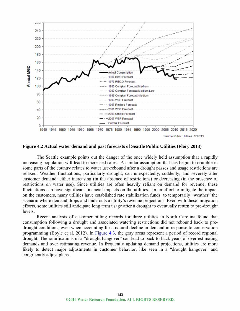
143
Figure 4.2 Actual water demand and past forecasts of Seattle Public Utilities (Flory 2013) The Seattle example points out the danger of the once widely held assumption that a rapidly increasing population will lead to increased sales. A similar assumption that has begun to crumble in some parts of the country relates to water use-rebound after a drought passes and usage restrictions are relaxed. Weather fluctuations, particularly drought, can unexpectedly, suddenly, and severely alter customer demand: either increasing (in the absence of restrictions) or decreasing (in the presence of restrictions on water use). Since utilities are often heavily reliant on demand for revenue, these fluctuations can have significant financial impacts on the utilities. In an effort to mitigate the impact on the customers, many utilities have established rate stabilization funds to temporarily “weather” the scenario where demand drops and undercuts a utility’s revenue projections. Even with these mitigation efforts, some utilities still anticipate long term usage after a drought to eventually return to pre-drought levels. Recent analysis of customer billing records for three utilities in North Carolina found that consumption following a drought and associated watering restrictions did not rebound back to pre-drought conditions, even when accounting for a natural decline in demand in response to conservation programming (Boyle et al. 2012). In Figure 4.3, the gray areas represent a period of record regional drought. The ramifications of a “drought hangover” can lead to back-to-back years of over estimating demands and over estimating revenue. In frequently updating demand projections, utilities are more likely to detect major adjustments in customer behavior, like seen in a “drought hangover” and congruently adjust plans.
©2014 Water Research Foundation. ALL RIGHTS RESERVED.

144
Figure 4.3 Changes in residential water use from 2007-2010 (Boyle et al. 2012); 6 month moving average residential water use
If utilities do not account for permanent, or even temporary, changes in consumption following
a drought, they run the risk of over-estimating use in months and years following a drought, and thereby over-projecting revenues from proposed rates. This may lead to setting rates too low due to not accounting for permanent declines in use, and subsequently collecting less revenue than projected. The risks of revenue shortfalls can be avoided once a utility has good information about the impacts and duration of drought-time curbs in water use (Boyle et al. 2011) Conclusion In an age of abundant data, its use can seem overwhelming, but water utilities have valuable assets in the data that they keep when extracted and analyzed. If detailed, integrated, and updated, demand forecasting can help water resource managers and finance officers make plans with more confidence and less financial risk.
References Austin Water Utility. 2011. Water Service Rates. Austin, Tex.: City of Austin. Beecher, J. 1996. Avoided cost: an essential concept for integrated resource planning. Water Research
and Education, 104(1): 28–35. Beecher, J. and T. Chestnutt. 2012. Declining Sales and Water Utility Revenues: A Framework for
Understanding and Adapting. A White Paper presented at the National Water Rates Summit, Racine, Wisc., October 24, 2012.
Billings, R.B. and C.V. Jones. 2008. Forecasting Urban Water Demand. Denver, Colo.: AWWA. Bishop, D.B. and Weber, J.A. 1996. Impacts of Demand Reduction on Water Utilities. Denver, Colo.:
AwwaRF. Boyle, C., S. Eskaf, M. Tiger and J. Hughes. 2011. Mining Water Billing Data to Inform Policy and
Communication Strategies. Jour. AWWA, 103(11): 45-58.
©2014 Water Research Foundation. ALL RIGHTS RESERVED.

145
Boyle, C. M. Tiger, M. Ngo, S. Eskaf and C. Wichman. 2012. Shifting Baselines in Water Management: Using customer-level analysis to understand the interplay between utility policy, pricing, and household demand. Chapel Hill, N.C.: Environmental Finance Center. Final report to the NC Urban Water Consortium. [Online]. Available: < http://dspace2.lib.ncsu.edu:8080/dr/handle/1840.4/8132> [cited October 31, 2013]
Chesnutt, T.W. & Beecher, J.A., 2004. Revenue Effects of Conservation Programs: The Case of Lost Revenue. Incomplete
DeOreo, W.B. and Mayer, P.W. 2012. Insights into declining single-family residential water demand. Jour. AWWA, 104(6): 383–394.
Fiorito, S., M. Gable and M. Topol. 2008. An empirical analysis of the components of retailer customer loyalty programs. International Journal of Retail and Distribution Management, 36(1): 32-49.
Flory, B. 2013. 2013 Revised Official Yield Estimate and Long-Range Water Demand Forecast. Seattle Public Utilities. [Online] Available at: <http://www.seattle.gov/util/Documents/Plans/Water/DemandForecast/index.htm.> [cited September 30, 2013]
Hoffner, J. 2008. Hidden Reservoir: Why Water Efficiency Is The Best Solution For The Southeast. Washington D.C.: American Rivers.
Hunter, M., K. Donmoyer, J. Chelius and G. Naumick. 2011. Declining Residential Water Use Presents Challenges, Opportunities. OpFlow, 37(5): 18-20.
Leurig, S. 2012. Water Ripples: Expanding Risks for U.S. Water Providers. Boston, Mass.: Ceres. Levin, E., W. Maddaus, N. Sandkulla, and H. Pohl. 2006. Forecasting Wholesale Demand and
Conservation Savings. Jour. AWWA, 98(2): 102-111. Rockaway, T.D., P.A. Coomes, J. Rivard and B. Kornstein. 2011. Residential water use trends in North
America. Jour. AWWA, 103(2): 76-89. ALTERNATIVE RATE DESIGNS Introduction: Challenges of Current Rate Structures
Water utilities consider much more than revenue recovery when setting the price of their product (e.g. customer affordability), and sometimes these considerations directly conflict with revenue stability and sufficiency objectives. One of the most notorious conflicts is between the goal of revenue stability and that of customer conservation and efficiency. The most prevalent retail pricing model in the industry relies on a modest base charge normally coupled with a much larger variable charge based on volumetric use. This highly variable structure provides an incentive for customer conservation and efficiency. Generally, the larger the ratio of variable revenue to fixed revenue, the greater the conservation incentive. In fact, members of the California Urban Water Conservation Council (CUWCC) are encouraged to recover at least 70% of revenue from variable charges, among other “best practices” designed to encourage customer conservation (CUWCC 2011). Ironically, the inverse ratio commonly holds true for the costs of a water utility. In its FY2012 Approved Budget, the Austin Water Utility divided each individual line item in their budget into fixed and variable costs (Austin Water Utility 2012). Figure 4.4 shows that 87% of their costs were projected to be fixed, while only 18% of their revenues were from fixed charges. The trend was similar for the Alameda County Water District and echoed across the project’s utility partners.
©2014 Water Research Foundation. ALL RIGHTS RESERVED.
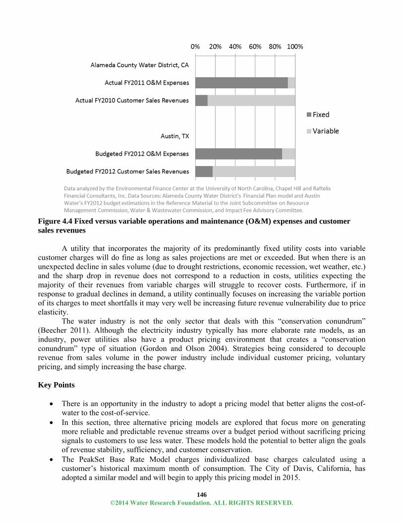
146
Figure 4.4 Fixed versus variable operations and maintenance (O&M) expenses and customer sales revenues
A utility that incorporates the majority of its predominantly fixed utility costs into variable customer charges will do fine as long as sales projections are met or exceeded. But when there is an unexpected decline in sales volume (due to drought restrictions, economic recession, wet weather, etc.) and the sharp drop in revenue does not correspond to a reduction in costs, utilities expecting the majority of their revenues from variable charges will struggle to recover costs. Furthermore, if in response to gradual declines in demand, a utility continually focuses on increasing the variable portion of its charges to meet shortfalls it may very well be increasing future revenue vulnerability due to price elasticity.
The water industry is not the only sector that deals with this “conservation conundrum” (Beecher 2011). Although the electricity industry typically has more elaborate rate models, as an industry, power utilities also have a product pricing environment that creates a “conservation conundrum” type of situation (Gordon and Olson 2004). Strategies being considered to decouple revenue from sales volume in the power industry include individual customer pricing, voluntary pricing, and simply increasing the base charge. Key Points
There is an opportunity in the industry to adopt a pricing model that better aligns the cost-of-water to the cost-of-service.
In this section, three alternative pricing models are explored that focus more on generating more reliable and predictable revenue streams over a budget period without sacrificing pricing signals to customers to use less water. These models hold the potential to better align the goals of revenue stability, sufficiency, and customer conservation.
The PeakSet Base Rate Model charges individualized base charges calculated using a customer’s historical maximum month of consumption. The City of Davis, California, has adopted a similar model and will begin to apply this pricing model in 2015.
©2014 Water Research Foundation. ALL RIGHTS RESERVED.
147
The CustomerSelect Model gives individual customers the choice to select an allotment of use that meets their needs and charges a fixed amount for that allotment for all use under it. Water use that exceeds the allotment is charged at a high rate.
The WaterWise Dividend Model basically ensures that utility cost recovery takes precedence, but returns “profit” to customers that use water efficiently.
Each pricing model explored needs additional research to gauge customer understanding, response, and technical feasibility.
Justifying an Alternative
Some studies have shown that customer efficiency can decrease long-term costs for utilities (Chesnutt and Beecher 2004, Hunter et al. 2011, Bishop and Weber 1996). But, in the short and medium term, water utilities are challenged to balance budgets and recover costs in the face of declining consumption. A high dependence on variable revenue can put these two planning timeframes in direct conflict with one another. Exclusively focusing on revenue stability in one single fiscal year – for example increasing base charges across the board and decreasing variable charges – may assure a level of revenue in the forthcoming year, but it concurrently diminishes price signals to customers to use water wisely and could lead to longer term costs linked to expansions that could have been avoided or delayed.
The foundation behind many water rates across the United States is the American Water Works Association’s M1 Manual on Principles of Rates, Charges, and Fees. This manual advocates cost-of-service ratemaking and describes several paths including the base-extra capacity method or the commodity-demand method. Both of these methods encourage a utility to think through the costs that fluctuate with total volume used and the rate at which it is used, but that doesn’t necessarily translate to a balanced cost and revenue situation year-to-year (AWWA 2012). In a recent water rate system evaluation, the City of Davis (California) utilized the commodity-demand method to determine that 56% of its total costs were associated with the quantity of water it produced (commodity). But they found that there is an important difference between costs that are “associated” with quantity of water produced and costs that actually fluctuate in short or medium term with water produced. An accounting exercise in Davis re-categorized well over half of its “commodity” costs as fixed and identified only 20% of the utility’s costs as truly variable in terms of annual budgeting (Williams 2013).
Cost-of-service studies are important in designing and explaining rate levels and structures. Utility commissions and governing boards look to these studies to assess sufficiency and fairness. Additionally, in the State of California, utilities must hold their rate structures against Proposition 218 which, among other requirements, requires “proportionality” in government’s fees and charges. The state requires that a fee or charge should not exceed the proportional cost of the service attributable to the parcel (League of California Cities 2007). But terms like fairness and proportionality are subjective. Rate consultants and utility staff may interpret these terms in a specific way; propose rates solidly based on that interpretation, and run into the conflicting interpretations from the rate-approving board.
There is an opportunity in the industry to adopt a pricing model that better aligns the cost-of-water to the cost-of-service. Modeling Alternatives
Most systems make general assumptions about the behavior and usage patterns of different customer classes and customers with different meter sizes to distribute utility costs. These classes are most often grouped based on common characteristics, such as single-family residential, multi-family
©2014 Water Research Foundation. ALL RIGHTS RESERVED.

148
residential, commercial, industrial, and irrigation; in rate modeling, costs are allocated to these customers through fixed and variable charges based in cost-of-service and proportionality principles. Typically, customers of the same “categorization” and/or meter size are charged the same base charge. But charging customers in these categories the same charge does not capture the diversity of demand provided within them, particularly in terms of their impact on a utilities’ capacity needs and fixed costs.
Figure 4.5 illustrates this point using the hypothetical demands of two families with the same average annual consumption, but vastly different system impacts. For example, a household with a large family on an urban lot that uses a moderately high, but steady amount of water throughout the year (Family 1) could pay the same base charge and same annual costs for water as a smaller family (Family 2) with a large suburban lot that uses a relatively small amount of water in the winter and twice as much during the summer irrigation. On average, the two families consume the exact same amount of water (72,000 gallons) per year. But rather than building a system that meets the sum of their average water use, the utility must build a system to meet the demands of Family 1 plus the peak of Family 2. In the wintertime, the capacity is still there, even if Family 2 is not using (and paying for) the water. Given the prevalent seasonal nature of water demand (particularly residential water demand), “the law of averages” does not always mitigate this phenomenon, but rather exacerbates it.
Figure 4.5 Hypothetical demands of two families with the same average annual consumption, but vastly different system impacts
The question therefore facing many utilities is how far to go tailoring what used to be standard
customer class features to the behavior of individual customers. By individually tailoring rates, utilities can better ensure that customers are billed for their specific demands on the system. Individually tailored rate structures are not in-and-of-themselves unique in the industry. Some utilities across the country use an individual customer’s average winter consumption to establish and apply tiered rate structures designed to target indoor and outdoor water use with different rates. Additionally, utilities with budget-based rates use a host of various individualized customer characteristics to establish a budget and relevant rates for customers. These two versions of rate structures do more to tailor charges to individual demands, but still place great reliance on variable charge.
As part of this research project, three alternative pricing models were explored that focused more on generating more reliable and predictable revenue streams over a budget period without
0
2
4
6
8
10
12
14
16
System
capacityrequirem
ents
Family2
Family1
Unused Capacity
Unused Capacity
©2014 Water Research Foundation. ALL RIGHTS RESERVED.

149
sacrificing pricing signals to use less water in an effort to better align the goals of revenue stability, sufficiency, and customer conservation.
The first two models presented below build more revenue recovery into fixed charges but annually tailor that fixed charge based on individual historical customer demand patterns. This model helps to close the short-term revenue gap that can leave a utility short-changed during a budget year. The third model basically ensures that utility cost recovery takes precedence, but rewards customers that use water efficiently. Concurrent to this project, the City of Davis (CA) was independently proceeding with an overhaul to their pricing model that introduces a formulaic and tailored base charge in response to a new surface water project and under the advisement of a stakeholder advisory group. A case study on this effort is also profiled to both illustrate a model and a process. Methodology
Historical billing records from two utilities (Beaufort-Jasper Water and Sewer Authority, SC and Clayton County Water Authority, GA) were used to model, for discussion purposes, two pricing structures. Neither utility had intentions to overhaul their pricing structure in the short term, however both organizations (like many of our partner utilities) had identified some weaknesses to existing pricing structures and were interested in assessing the impact of potential new models on their finances and customers. (Interestingly enough, when presented with the choice pricing structures to model in-depth, the utilities each chose different models.) Applying different pricing models to a robust data set of actual customer usages allowed the development of revenue-neutral pricing models that shifted revenue generation across customers and months of the year. Moreover, utilities were directly engaged in setting the rate-levels of each model. There are a multitude of underlying assumptions built into both models that influence the specific rates levels. The purpose of the following descriptions is not to focus on the specific charges but on the underlying structure and implications of that structure. PeakSet Base Model
The PeakSet Base Rate Model charges individualized base charges calculated using a
customer’s historical maximum month of consumption. This theoretical model is inspired by power utilities’ demand ratchet charges, yet grounded in the limitations of prevalent water metering technology6. Under this rate structure, a customer’s base charge would be individually set based on a three-year rolling average of that customer’s peak month of demand. The utility would still charge variable commodity charges, but they would constitute a lower proportion of a customer’s bill. This model would allow a utility to build more of their cost recovery into the base charge while still promoting customer conservation and efficiency. In particular, it would encourage consistent customer water use, benefitting both the utility and its customers through reduced financial risk for utility and increased financial predictability for its customers.
Table 4.2 below compares Beaufort-Jasper’s (BJWSA) current meter-size-dependent base charge plus a uniform variable rate to a hypothetical revenue-neutral PeakSet Base structure. Under the PeakSet Base residential rate structure, the utility would tailor each customer’s base charge for the forthcoming year using the average of the previous three years’ peak monthly consumption.
6 Utilities with Advanced Metering Infrastructure (AMI) would be able to adapt this model to target peaks in daily demand.
©2014 Water Research Foundation. ALL RIGHTS RESERVED.
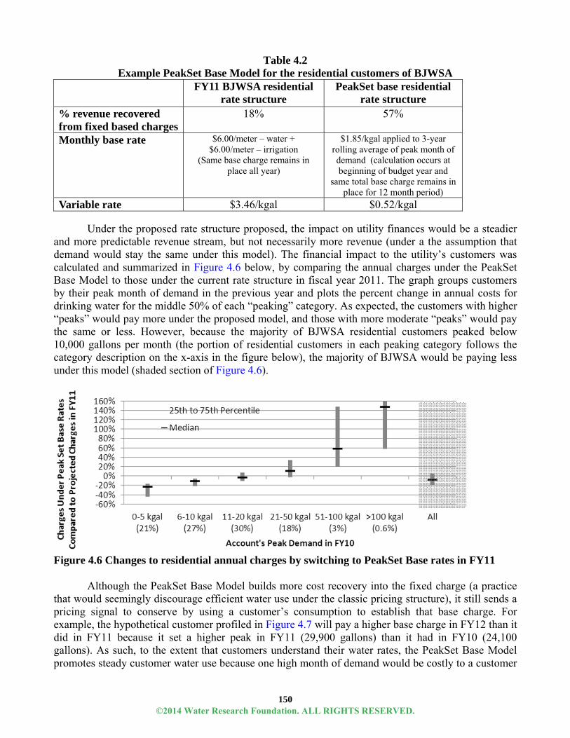
150
Table 4.2 Example PeakSet Base Model for the residential customers of BJWSA FY11 BJWSA residential
rate structure PeakSet base residential
rate structure % revenue recovered from fixed based charges
18% 57%
Monthly base rate
$6.00/meter – water + $6.00/meter – irrigation
(Same base charge remains in place all year)
$1.85/kgal applied to 3-year rolling average of peak month of demand (calculation occurs at beginning of budget year and
same total base charge remains in place for 12 month period)
Variable rate $3.46/kgal $0.52/kgal
Under the proposed rate structure proposed, the impact on utility finances would be a steadier and more predictable revenue stream, but not necessarily more revenue (under a the assumption that demand would stay the same under this model). The financial impact to the utility’s customers was calculated and summarized in Figure 4.6 below, by comparing the annual charges under the PeakSet Base Model to those under the current rate structure in fiscal year 2011. The graph groups customers by their peak month of demand in the previous year and plots the percent change in annual costs for drinking water for the middle 50% of each “peaking” category. As expected, the customers with higher “peaks” would pay more under the proposed model, and those with more moderate “peaks” would pay the same or less. However, because the majority of BJWSA residential customers peaked below 10,000 gallons per month (the portion of residential customers in each peaking category follows the category description on the x-axis in the figure below), the majority of BJWSA would be paying less under this model (shaded section of Figure 4.6).
Figure 4.6 Changes to residential annual charges by switching to PeakSet Base rates in FY11
Although the PeakSet Base Model builds more cost recovery into the fixed charge (a practice
that would seemingly discourage efficient water use under the classic pricing structure), it still sends a pricing signal to conserve by using a customer’s consumption to establish that base charge. For example, the hypothetical customer profiled in Figure 4.7 will pay a higher base charge in FY12 than it did in FY11 because it set a higher peak in FY11 (29,900 gallons) than it had in FY10 (24,100 gallons). As such, to the extent that customers understand their water rates, the PeakSet Base Model promotes steady customer water use because one high month of demand would be costly to a customer
©2014 Water Research Foundation. ALL RIGHTS RESERVED.

151
for the forthcoming years. As shown in Figure 4.7, it also benefits the customer with relatively stable payments within a given year.
Figure 4.7 Comparison of monthly and annual charges under the current rate structure to PeakSet Base-modeled rates for the same amount of water use
As modeled in Table 4.2, however, the utility would continue to send a variable price signal
(albeit much smaller) every month to send immediate feedback on water use. (Figure 4.7 shows a slight variation in the monthly charges.) There may be debate that behavior in a given year that influences what a customer pays the following year is too indirect to influence usage; this would be an interesting research topic to study. The use of new smart meters and customer communication tools such as text messaging reminders to customers approaching their peak or exhibiting other behavior could help compensate for the time lag in expenditure.
There are some challenges to implementing and executing this pricing model. For example, it was challenging to extract sufficient data from the utility’s billing system to determine a three-year rolling peak that would establish a customer’s base charge. This could be a challenge for other utilities in establishing this rate structure. Additionally, there would be issues in dealing with new and moving customers. How would a utility determine the base charge for a customer with no historical record? The Water Advisory Committee in Davis, California considered this last question and recommended that the utility either use the historical usage of a previous occupant, adopt an average customer profile, or allow a customer to establish their usage profile themselves, and then settle up at the end of the year (Williams 2013). Utilities with budget-based rates have grappled with similar issues and developed similar methodologies. For example, Athens-Clarke, Georgia (a college town) calculates the water budget for new residential customers using a two-person household with an average use of 50 gallons a day per person. Households with more customers can request adjustments.
As with any pricing structure, there are potential weaknesses to this structure. For example, a customer that is planning to move would not have as strong a financial incentive to control their behavior since the most important cost impact of their behavior would not be triggered until after they were gone. Moreover, a utility that implements a PeakSet Base Model should anticipate more meter re-reads and high bill disputes as customers realize the long-term implications of a high meter read, if they understand it at all. Again, customer understanding would be another interesting topic to explore.
©2014 Water Research Foundation. ALL RIGHTS RESERVED.

152
Case Study
The Consumption-Based Fixed Revenue Water Rate System in Davis, California. In 2012, the Davis City Council appointed a Water Advisory Committee to develop the most “fair” way to charge its water customers for the costs of the new surface water project; the Woodland-Davis Clean Water Agency project was estimated to cost the Town of Davis $113 million. It involves pumping water from the Sacramento River, treating it, and piping it to Davis and Woodland in an effort to supplement a deteriorating ground water source (Resolution No. 11-193, Series 2011).
The Committee was charged to propose a rate to the Davis City Council that balanced the requirements of the state’s Proposition 218 (that requires water service fees to be “proportional” to the cost of providing water service) and the requirements of Article X, Section 2 of the state Constitution (that requires that the water resources of the state be conserved and the waste or unreasonable use of water prevented). At the same time, the group had to consider the fixed cost of the debt the City would incur to finance this new project and propose a rate structure that would cover it.
The rate structure proposed by the Committee to the City Council and community of Davis works similarly to the PeakSet Base Rate Model described above in that a customer’s historical water use is used to establish their fixed charge in the forthcoming year. In addition to the fixed charge, customers would be charged a variable rate through an increasing block rate structure, as well as a “readiness to serve” fixed charge that is based on the size of a customer’s meter (Niederberger and Jensen 2013).
Proponents of the consumption-based fixed revenue rate model argue that the model is more “proportional” because the base charge is related to actual, rather than potential system demand. They also argue that it promotes water conservation because the base charge is set by demand concurrent to system demand. Opponents of the rate model, represented in a legal challenge to the City as the Yolo Ratepayers for Affordable Public Utility Services, argue that customers that use the same amount of water will be charged different amounts and that it violates the “proportionality” required by the state’s Proposition 218 (Sakash 2013). At the time this report was published, the City plans to launch the consumption-based fixed revenue water rate system in 2015 to give the utility time to communicate the nuances of the rate model and the long-term financial ramifications of a customer’s water use. CustomerSelect Model
The second alternative pricing model studied was the CustomerSelect Model. The CustomerSelect Model gives individual customers the choice to select an allotment of use that meets their needs and charges a fixed amount for that allotment for all use under it. If the customer exceeds that allotment in a given month, the utility charges a punitive overage fee. In many ways, the CustomerSelect Model is similar to a budget-based rate structure , but rather than establishing the budget parameters for customers, it gives customers autonomy to choose their own budget. Potential benefits of this model include increased revenue stability because customers commit to plans. In addition, by giving the customer the choice, the utility does not have the administrative burden of assigning customers to budgets, as they would with a budget-based rate structure. It promotes water-use efficiency, especially around the plan’s “break points.” Furthermore, it moves the pricing structure towards one focused on water and sewer service rather than a commodity.
©2014 Water Research Foundation. ALL RIGHTS RESERVED.

153
Table 4.3 below compares the range of charges to residential customers under the rate structure of the Clayton County Water Authority (GA) in 2011 to a revenue-neutral option for structuring a CustomerSelect rate7.
Table 4.3 Modeled water and irrigation schedule for CustomerSelect Model
Plan name* Monthly water allotment
Charge under 2011 rate structure
CustomerSelect base charge
Overage charge
Lifeline 2,000 gallons $8.93-$13.13 $8.13 $6.83/kgal
Basic service/Small family
6,000 gallons $15.23-$30.38 $18.70 $6.83/kgal
Light irrigation/Large family
10,000 gallons $35.43-$54.18 $32.52 $6.83/kgal
Heavy irrigation 24,000 gallons $64.75-$146.68 $81.30 $6.83/kgal
Water waster unlimited >$154.18 $162.60 NA
*Plan names are simply meant to be illustrative.
The rate was modeled assuming that customers would select their plan based on their historical average water use. The graph below shows how many residential customers would have, on average, exceeded their plan (as hypothetically laid out above) in FY 11 as determined by FY10 average water use. If residential customers selected their FY11 CustomerSelect Plan purely based on their own average in FY10, 18% would have exceeded their Plan's allotment on average (based on their FY11 use). This is displayed in Figure 4.8. One note to consider in the details of this model is that it was modeled retrospectively to back into a revenue neutral rate. Should a utility design this structure under projections and assumptions for the forthcoming year, they might want to align the base charge revenue with fixed costs and the overage charge revenue with the variable costs.
Figure 4.8 Changes in average use by residential customers from FY10 to FY11
7 The actual charges associated with each plan were developed in collaboration with utility officials in Clayton County Water Authority. The levels, of course, could and would be adjusted to suit utility‐specific objectives and politics.
©2014 Water Research Foundation. ALL RIGHTS RESERVED.

154
The CustomerSelect Rate model has the potential to stabilize utility rates by “locking”
customers into plans. Under the modeled rate structure, the Clayton County Water Authority would have collected 85% of its retail revenue from base charges, as opposed to 32%. Additionally, it is a relatively simple model to understand and advances the utility as a provider of a service. Customers would have an incentive to keep their consumption below the break-point of their plan and even to move down to a lower plan the next year. As with the PeakSet Base Model, it is easy to envision a role for new smart meter and customer notification technology with this structure. Providing customers with frequent updates on their usage during a billing period may make customers more aware of the water they use, but it also could signal to some customers a license to waste water at the end of some months just because they can at no extra cost.
This model does introduce social science questions that may be difficult to account for in the budgeting process. How will utilities predict what plans customers will choose? The model was generated under the assumption that households would use their historic average to choose a plan, but households that teeter on either ends of the breaks may choose to be conservative or liberal with their plan. If a utility has not invested in smart meter technology it may have to – as customers are likely to demand real-time water use information so that they can track their consumption against their block. Additional refinement of the plan will further consider the economic and social incentives and dis-incentives embedded in the model. For example, it has been pointed out that the pricing model gives a lower per-unit price to the customer that uses the maximum allowed under a Plan versus the lowest plan (Beecher 2012). Pilot applications of the rate model should focus on customer plan selection and the impact on demand.
WaterWise Dividend Model
Owned by their members, some cooperative retail organizations return profit to their “owners”
once financial obligations are met. Many times these cooperatives return larger “dividends” to the “owners” that bought more of their product over time. Under the theoretical WaterWise Dividend Model, water utilities seeking revenue stability and efficient customers would adopt an adapted model. However, rather than rewarding customers that used more, they would return conservation dividends to customers that used less or used water in a way that minimized short or long term costs. The definition of “less” could be established against a customer’s budget (for those utilities with budget-based rates) or relative to an individual customer’s historic use. Moreover, they could calculate a dividend according to any number of policies the utility wanted to promote, such as “peak shaving.”
This model has the benefit of communicating to customers that the utility is a not-for-profit entity (in cases where this is true), as “profits” are returned to customers. It provides a positive way for utilities to interact with their customers (much like rebate programs) and it helps ensure that the financial goals are met above other priorities. It has even been extoled by utility officials as a valuable, temporary tool to use when adopting a new rate structure to assure customers of a new rate’s revenue-neutral intent.
Returning money to citizens is not unprecedented. In January 2013, DC Water announced that it would refund a one-time credit to customer bills because it finished Fiscal Year 2012 with a surplus (DC Water 2013). They anticipated a total system refund of $4.2 million at a rate of $0.10 per ccf and $1 per ERU (equivalent residential unit). Even though, this rebate was given to customers that use more, the model could be adopted and the formula adjusted.
At this point, this model is more theoretical in nature; it has not been extensively modeled. It was, however, presented informally to a panel of water utility finance experts at the American Water Works Association’s Annual Conference and Exposition in the summer of 2012. These experts included Doug Scott, Managing Director of Fitch Ratings’ US Public Finance Group; Janice Beecher,
©2014 Water Research Foundation. ALL RIGHTS RESERVED.
155
Director of the Institute of Public Utilities at Michigan State; and Jeff Walker, Director of Project Development for the Texas Water Development Board. The panel expressed hesitation about a few components of this model, including giving money back to customers, stressing the point that this model is only likely to succeed with a utility that maintains a conservative finance policy and meets goals before writing any checks. Conclusion: Implementing Alternatives
The models described above have theoretical validity in meeting objectives of revenue sufficiency, stability, and customer conservation. But in reality, most governing boards and utility managers are hesitant to blaze a trail, especially on an initiative that significantly alters the way revenue is earned and customers are charged. In discussion, eighteen utility leaders identified challenges that needed be addressed before their utility could move forward with an overhaul to their utilities’ pricing model. Their responses communicated the challenging, but not insurmountable, process of transforming a utility’s business practices.
Some saw technical challenges. They recognized that their current metering and billing technology were not sophisticated enough to communicate real-time water usage information likely to be demanded under the CustomerSelect Model or to individually calculate base charges off a customer’s historical demand under the PeakSet Base Model.
Others felt like the models needed more standardization on how the industry should approach pricing transformation and a bit of tweaking to make them simpler. The utility officials proposed questions like what to do with new customers that have no demand history when setting a PeakSet Base Charge. And they needed better assurance that the models would actually generate revenue neutral rates: no massive surpluses, no scary deficits.
Overwhelming, though, the utility officials expressed a need for a well-executed communication and education campaign – more investigation into how customers would understand, receive, and react to these models. Even before going to the customers, utility officials expressed a need for stakeholder and board communication. Getting stakeholder and board buy-in to a rate structure that has the potential to significantly alter customers’ monthly bills is no insignificant contest. A revenue-neutral overhaul of the status quo will undoubtedly result in lower costs for some customers and higher costs for others. Those that will receive higher costs are likely to object openly and loudly. But overwhelmingly, the utility officials asked, “how will these rate structures actually influence customer demand and utility revenues?” Elasticity of long-term water demand (as opposed to responses to monthly pricing signals) has not been tested and assumes a level of customer understanding of the rates.
The headline of a story in the Davis Enterprise the morning after the Council voted to move forward with the Consumption-Based Fixed Revenue Rate Model read “Council to consider untested rate model (Sakash 2012).” At this point, they have cleared many of the administrative hurdles and initiated a communication strategy. If the courts support the rate’s proportionality, Davis officials will have blazed a trail for other utilities to watch and follow.
References Austin Water Utility. 2012. FY2012 Approved Budget, Fixed and Variable Costs. Austin, Tex.: City of
Austin. [Online]. Available: <http://www.austintexas.gov/sites/default/files/files/Water/awu2012lineitemfixedvsvariablecosts11302011.pdf> [cited May 1, 2013]
AWWA (American Water Works Association). 2012. M1 Manual: Principles of Water Rates, Fees, and Charges. Denver, Colo.: AWWA
©2014 Water Research Foundation. ALL RIGHTS RESERVED.

156
Beecher, J. 2011. The Conservation Conundrum: How Declining Demand Affects Water Utilities. Jour. AWWA, 102(2): 78-80
Beecher, J. 2012. August 28 (1:49 p.m.). comment on Christine E. Boyle, CustomerSelect Rate Plan: How would a cell phone rate plan work for water service? The Environmental Finance Center Blog. [Online]. Available: <http://efc.web.unc.edu/2012/08/28/customerselect-rate-plan-how-would-a-cell-phone-rate-plan-work-for-water-service/> [cited May 1, 2013]
Bishop, D.B. and Weber, J.A. 1996. Impacts of Demand Reduction on Water Utilities. Denver, CO: AwwaRF.
CUWCC (California Urban Water Conservation Council). 2011. Memorandum of Understanding Regarding Urban Water Conservation in California. Sacramento, Calif.: CUWCC. [Online]. Available: <http://www.cuwcc.org/mou-main-page.aspx> [cited May 1, 2013]
Chesnutt, T.W. and Beecher, J.A. 2004. Revenue Effects of Conservation Programs: The Case of Lost Revenue. White Paper. Los Angeles, Calif.: A&N Technical Services, Inc. [Online]. Available: http://www.allianceforwaterefficiency.org/WorkArea/linkit.aspx?LinkIdentifier=id&ItemID=1048 [cited May 8, 2013]
DC Water. 2013. What’s on TAP: News for DC Water Customers, 14(1). Washington D.C.: District of Columbia Water and Sewer Authority. [Online]. Available: <http://www.dcwater.com/news/publications/WOT_JAN_web.pdf> [cited May 1, 2013]
Donnelly, K., J. Christian-Smith, and H. Cooley. 2013. Pricing Practices in the Electricity Sector to Promote Conservation and Efficiency: Lessons for the Water Sector. [Online]. Available:<http://www.pacinst.org/wp-content/uploads/2013/09/pacinst-pricing-practices-full-report.pdf> [citied October 31, 2013]
Gordon, K. and W. Olson. 2004. Retail Cost Recovery and Rate Design in a Restructure Environment. Washington D.C.: Edison Electric Institute.
Hunter, M., K. Donmoyer, J. Chelius and G. Naumick. 2011. Declining Residential Water Use Presents Challenges, Opportunities. OpFlow, 37(5): 18-20.
League of California Cities. 2007. Proposition 218: Implementation Guide. Sacramento, Calif.: The League of California Cities. [Online]. Available: <http://www.cacities.org/UploadedFiles/LeagueInternet/e0/e0ae1157-b743-455f-a6a8-9e8f22537974.pdf> [cited May 1, 2013]
Niederberger, H. and D. Jensen. 2013. Staff Report to [Davis, California] City Council regarding Water Rate Recommendation. [Online]. Available: http://city-council.cityofdavis.org/Media/Default/Documents/PDF/CityCouncil/CouncilMeetings/Agendas/20130115/06-Water-Rate-Recommendation.pdf [cited September 27, 2013]
O’Donnel, P. 2008. Dominion’s fixed charge could rise 200 percent. Posted on Cleveland.com Blog, July 5.[Online]. Available: <http://blog.cleveland.com/business/2008/07/dominions_fixed_charge_could_r.html> [cited May 1, 2012]
Resolution No. 11-193, Series 2011. Resolution of the City Council of the City of Davis Establishing the Structure and Purpose of the Water Advisory Committee. [Online]. Available: http://archive.cityofdavis.org/meetings/water-advisory/documents/2011-12-08-item5-water-advisory-committee-authorizing.pdf [cited September 27, 2013]
Rockaway, T.D., P.A. Coomes, J. Rivard and B. Kornstein. Residential water use trends in North America. Jour. AWWA, 103(2): 76-89.
Sakash, T. 2012. Council to consider untested rate structure. The Davis Enterprise, December 19. [Online]. Available: < http://www.davisenterprise.com/local-news/city/council-to-consider-untested-water-rate-structure/> [cited May 1, 2012]
©2014 Water Research Foundation. ALL RIGHTS RESERVED.
157
Sakash, T. 2013. City sued over water rates, use. The Davis Enterprise, February 1. [Online] Available: http://www.davisenterprise.com/local-news/city/city-sued-over-water-rates-use/ [cited September 27, 2013]
Williams, Matt (Alternate on Water Advisory Committee). 2013. Interview by Mary Tiger. Telephone. Chapel Hill, N.C., February 8, 2013.
RATE STABILIZATION RESERVES
Introduction
Reserve funds have become an increasingly important part of a water utilities’ efforts to ensure financial stability and resiliency. Water utilities normally operate as enterprises without outside assistance from a city or local government. Operating revenues from fixed and variable charges directly support the utility and comprise the bulk of utility revenues. Due to fluctuations in the economy, weather, and other unexpected events, utilities need to have adequate financial planning, which typically involves reserves of money set aside to be used for hedging risk. Most utilities, however, operate as “not for profit” businesses, and water rates are often restricted by local governments or utility commissions so that customers are not overcharged. This creates a need for utilities to have one or more reserve funds appropriated for different types of expenditures, which can be justified to a local government or utility commission.
These reserves are used to create a monetary buffer to offset the financial risks of unforeseen natural events, infrastructure repairs, and facility upgrades (Mann 2010). “Appropriate” sizing of reserve funds is critical, yet reserve fund targets vary widely among utilities. This section will explore how a number of utilities are using reserve funds and identify targets in-place for these reserves. It will also serve as a discussion of the functional role of reserve funds, as well as issues presented by partner utilities, credit rating agencies, and other stakeholders. Key Points
There are four major purposes for reserve funds: o Contingency Planning o Achieve or maintain good standing with credit rating agencies, and subsequently benefit
from lower borrowing costs o Investment o Provide cash availability to cover lost revenues or to correctly time entrance into the
bond market Water utilities have two general types of reserves: restricted and unrestricted. Unrestricted
reserves can be designated, which carries varying associated requirements depending on the utility and its state.
Geography, weather, governance, and political priorities can affect reserve fund sizes and use. It is important for utilities to plan how resources will be set aside for each unrestricted reserve
fund balance, and to put in place mechanisms to protect unrestricted reserves. Reserve levels appear related to rate “smoothing.” While rate increases were not necessarily
smaller for utilities with higher reserve levels than other utilities, they tended to fluctuate less. Utilities with lower reserve levels (relative to operating expenses and debt service) had more volatile rate increases than those with larger reserve fund ratios.
There are three primary factors that can be used for reserve comparison between utilities: o The number and type of reserve funds
©2014 Water Research Foundation. ALL RIGHTS RESERVED.

158
o The amount of money in each reserve fund o Policies on how the reserve funds are utilized
Among our partner utilities, some have few designated reserve funds, while others have many. A portion of the utilities prefer to have fewer reserve funds, each with multiple uses and more flexibility of funds, and others prefer to have several different funds each with very specific uses. In our analysis of utility partner data, there was no correlation between the number of reserve funds, and debt service coverage ratio, days of cash on hand, or operating ratio. Additionally, the ratio of the total amount in these reserve funds to the sum of operation & maintenance costs and debt service costs, varied widely between utilities, pointing to precipitous differences in reserve fund policy.
Purpose In Financial Policies: Design and Implementation, Kavanagh et al. (2004) describe four major
purposes for reserve funds. The first and primary purpose is to plan for contingencies. Because almost all utilities rely on volume-based pricing structures, revenues are somewhat variable and may not closely match utility expenditures within a given year. This volatility in revenue, coupled with unexpected weather-related events, can drastically increase costs and create wide gaps between utility expenses and revenue. This uncertainty within water and sewer utility finance creates significant need of reserve funds.
The second major purpose of reserve funds is to achieve or maintain a good standing with credit rating agencies, and subsequently benefit from lower borrowing costs. Simply put, rating agencies use reserve funds as an indicator of financial health because financial reserves increase a utility’s ability to pay off debt. However, these agencies also take into account the ways in which reserves are used. Depletion of a reserve fund, for example, may be viewed unfavorably by a rating agency even if the reserve fund was depleted for a utility-designated reason, particularly if there is not a plan to replenish the fund. The use of reserve funds by credit rating agencies is further discussed in the “Rate Stabilization Fund” section below.
A third purpose of having reserve funds is that they can be invested. Treasury bills are a common, low-risk investment among municipalities, and investing a reserve fund can provide utilities with additional revenue. The Alameda County Water District (2009), for example, has a very broad investment policy that states that the district can invest funds “in a prudent manner which will provide the highest investment return with the maximum security of principal while meeting the daily cash flow demands of the District”. Clayton County Water Authority’s (2011) investment policy provides similar guidance, but states that investments must have maturity dates greater than 90 days, and earnings must be maximized without decreasing principle. There are limits to the level of risk of investments so many utilities are restricted to investments with returns that are very low at this time. As a result, this purpose has little value in times when investment income is very low.
Lastly, reserve funds can provide cash availability when revenues fall short. A reserve fund may be designated specifically for cash flows, so that a utility has access to additional money when revenues are low or there is seasonal variability in revenue generation. Also related to cash flow, reserve funds can allow utilities to better time their entrance into the bond market. These funds can then be replenished once the bond sale is complete (this often requires a reimbursement resolution). Types
Water and sewer utilities have two general types of reserve funds (restricted and unrestricted),
though the use of these reserve funds varies widely from utility to utility. Restricted funds refer to
©2014 Water Research Foundation. ALL RIGHTS RESERVED.
159
those funds that must be used for specific purposes. They include legally binding reserve fund balances for various categories that are set by state governments. Unrestricted reserve funds, however, are available for appropriation and can be divided into both designated and undesignated categories. Designated reserves are available for spending, but have been earmarked by utility managers (and potentially its governing board) for use for a specific purpose. The American Institute of Certified Public Accountants’ audit guide recommends that designated, unrestricted reserve funds have a definitive purpose and (at least) be approved by a utility’s senior management. Designations for these funds tend to be for capital improvement projects, unknown contingencies, or appropriations for the next year’s budget. While these funds may not technically be restricted, certain “designated” funds may be somewhat regulated depending on the state and interpretation of regulations. In North Carolina, capital reserve fund policy states:
“Any local government or public authority may establish and maintain a capital reserve fund for any purposes for which it may issue bonds. A capital reserve fund shall be established by resolution or ordinance of the governing board which shall state (i) the purposes for which the fund is created, (ii) the approximate periods of time during which the moneys are to be accumulated for each purpose, (iii) the approximate amounts to be accumulated for each purpose, and (iv) the sources from which moneys for each purpose will be derived” (Capital Reserve Funds 1971). The implications of this statute are that capital reserve funds (which are typically designated),
become more like restricted funds; however, it leaves some room for interpretation and the line between a designation and a restriction becomes somewhat blurred. Undesignated unrestricted reserve funds are available for spending and their use has not been designated for a particular purpose by the management. This type of fund is typically a good indicator for how flexible a utility can be when dealing with a financial emergency (Kavanagh et al. 2004).
Targets and Governance
Restrictions on reserve funds vary greatly from utility to utility. Geography, weather,
governance, and political priorities can affect reserve fund sizes and regulation. The Government Finance Officers Association (GFOA) recommends establishing minimum reserve fund levels, and many utilities have specific reserve policies based on expected revenues for the following year. Reserve targets can be either relative (a percentage or cost or revenues) or absolute (a specific dollar amount). Relative targets are more common and examples are described below. Table 4.4 shows only one (out of six) absolute target.
The City of Minneapolis, for example, dictates that a minimum of fifteen percent of the revenue budget for the next year be put into an unallocated general fund for cash flow, unexpected expenses, increases in service costs, and to maintain a AAA bond rating (GFOA 2013). Orange Water and Sewer Authority in Orange County, NC sets the target level of their operating reserves at the larger of 33% of their operating and maintenance budget or 20% of the total estimated cost of the three succeeding years of the CIP budget. Conversely, the Baltimore Department of Public Works dictates that a minimum of 90 days cash on hand be in their operating reserves. GFOA recommends maintaining an unrestricted fund balance of at least two months of operating revenues or expenditures. These and other reserve fund targets from the project’s utility partners are shown in Table 4.4, below.
©2014 Water Research Foundation. ALL RIGHTS RESERVED.

160
Table 4.4 Utility reserve fund targets
Utility Reserve Fund Targets City of Minneapolis1 15% of revenue budget for the next year Orange Water and Sewer Authority2 The greater of 33% of O&M budget or 20% of
the total estimated cost of the succeeding 3 years of the CIP budget
Baltimore Dept. of Public Works3 Minimum of 90 days cash on hand Alameda County Water District4 Sufficient to meet operating, capital, and debt
service obligations Charlotte-Mecklenburg Utilities5 100% of operating expenses for the current
budget Water District No.1 of Johnson County6 The Board will be notified when the rate
stabilization reserve reaches a minimum level of $2 million
1Source: GFOA, 2013 2Source: OWASA, 2009 3Source: Baltimore Department of Public Works, 2007 4Source: ACWD, 2009 5Source: CMUD, 2011 6Source: Water District No.1 of Johnson County, 2009 When setting policies for maintaining minimum reserve fund balances, several factors should
be taken into account, including the volatility of revenues and expenditures, the perceived exposure to financial risk (from natural disasters, drought, unexpected infrastructure repair, etc.), the amount of money and potential drain on other reserve funds, liquidity, and financial commitments to designated reserve funds (GFOA 2009). Another consideration when setting unrestricted reserve fund sizes is the size of a utility’s budget. Kavanagh et al. (2004) recommend that a government’s unrestricted reserve fund level on a relative basis be inversely proportional to the size of its total budget. For example, a smaller utility may be more susceptible to financial risk and economic changes and thus, may require larger relative reserve funds. Additionally, a reserve fund’s purpose may also influence its size. A hurricane-prone coastal community may have need of a larger contingency fund than a utility without a history of frequent natural disaster. Table 4.5, below, lists commonly used reserve funds along with some considerations for fund sizing.
©2014 Water Research Foundation. ALL RIGHTS RESERVED.

161
Table 4.5 Reserve fund size considerations
Reserve Fund Type Size Considerations Rate Stabilization Revenue variability (possibly due to seasonal variability,
increased precipitation, drought, conservation, etc.) Operating Capital Likelihood of a natural disaster, economic downturn,
financial shortfalls or other contingency Renewal and extension reserves Timeline for expansion or replacement, infrastructure age Capital project reserves Type of capital project (i.e. water supply expansion,
facility upgrades), timeline for when projects become necessary
Insurance reserves Likelihood of disaster or unforeseen event, infrastructure age, location & climate
It is also important for utilities to plan how resources will be set aside for each unrestricted
reserve fund balance, and to put in place mechanisms to protect unrestricted reserves. Politicians, city government leaders, and even savvy citizens may not fully understand the need for adequate reserves and may see it as a utility hoarding funds. Government leaders are often tempted to deplete a utility’s reserve fund to meet other financial needs or meet political goals, as was seen in the City of Park Ridge, IL. In 2010, against the recommendations of utility managers, the city council depleted utility reserve funds to pay for other expenses, noting that the reserve level was excessive (Mann 2010). This example indicates the importance of setting policies (and ideally seeking board-approval for those policies) for unrestricted fund balances, so that utilities can easily justify reserve levels to local governments. Conversely, some utilities may be keeping too much money in reserve funds, thereby charging customers a higher rate than necessary. It is difficult, however, to determine when a utility is retaining too much money in reserve funds. Figure 4.9 indicates reserve fund levels for each of our partner utilities, providing the ratio of total reserve funds to total operating expenses and debt service for each utility for one fiscal year.
©2014 Water Research Foundation. ALL RIGHTS RESERVED.
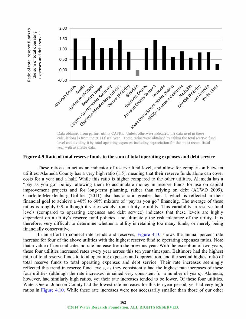
162
Figure 4.9 Ratio of total reserve funds to the sum of total operating expenses and debt service
These ratios can act as an indicator of reserve fund level, and allow for comparison between
utilities. Alameda County has a very high ratio (1.5), meaning that their reserve funds alone can cover costs for a year and a half. While this ratio is higher compared to the other utilities, Alameda has a “pay as you go” policy, allowing them to accumulate money in reserve funds for use on capital improvement projects and for long-term planning, rather than relying on debt (ACWD 2009). Charlotte-Mecklenburg Utilities (2011) also has a ratio greater than 1, which is reflected in their financial goal to achieve a 40% to 60% mixture of “pay as you go” financing. The average of these ratios is roughly 0.9, although it varies widely from utility to utility. This variability in reserve fund levels (compared to operating expenses and debt service) indicates that these levels are highly dependent on a utility’s reserve fund policies, and ultimately the risk tolerance of the utility. It is therefore, very difficult to determine whether a utility is retaining too many funds, or merely being financially conservative.
In an effort to connect rate trends and reserves, Figure 4.10 shows the annual percent rate increase for four of the above utilities with the highest reserve fund to operating expenses ratios. Note that a value of zero indicates no rate increase from the previous year. With the exception of two years, these four utilities increased rates every year across this ten year timespan. Baltimore had the highest ratio of total reserve funds to total operating expenses and depreciation, and the second highest ratio of total reserve funds to total operating expenses and debt service. Their rate increases seemingly reflected this trend in reserve fund levels, as they consistently had the highest rate increases of these four utilities (although the rate increases remained very consistent for a number of years). Alameda, however, had similarly high ratios, yet their rate increases tended to be lower. Of these four utilities, Water One of Johnson County had the lowest rate increases for this ten year period, yet had very high ratios in Figure 4.10. While these rate increases were not necessarily smaller than those of our other
Ratio of total reserve funds to
the sum of total operating
expen
ses and deb
t service
©2014 Water Research Foundation. ALL RIGHTS RESERVED.

163
partner utilities, they tended to fluctuate less. Utilities with smaller ratios in Figure 4.10 had more volatile rate increases than those with larger reserve fund ratios.
Figure 4.10 Annual percent rate increases for utilities with high reserve fund to operating expenses ratios
While there are many different types of policies regarding funding unrestricted reserves, many
utilities use specific formulas, percentages of operating surplus, or revenues from a specific source to help fund reserves to the target level. Formulas typically indicate that a small percentage of operating expenses go to unrestricted reserves. Other utilities require that a portion of operating surpluses be set aside for unrestricted reserves. This method is often useful for utilities with “pay as you go” financing. Another method for funding unrestricted reserves is to dictate that these reserves be funded only through revenue from a specific source, such as connection fees. This approach controls the amount that can be included in the reserve fund (Kavanagh et al. 2004). Trends in Reserves
Although utility reserve types, levels, and policies vary widely among utilities, there are three primary factors that can be used for reserve comparison between utilities:
The number and type of reserve funds The amount of money in each reserve fund Policies on how the reserve funds are utilized
©2014 Water Research Foundation. ALL RIGHTS RESERVED.

164
These factors will serve as a basis for discussion on reserve funds, in the context of the project’s utility partners.
Number and Types of Reserve Funds
Utilities often have a number of different reserve funds. While the number and type of reserve funds depends on a utility’s specific needs and policies, there are a few types of reserve funds that are frequently utilized. These funds, however, are used in different ways from utility to utility and often serve multiple purposes. The below paragraphs detail these commonly-used reserve funds and how they are used and regulated differently between our partner utilities.
Debt Service Reserves. Debt service reserves are one of the most commonly used reserve funds, and are typically restricted by bond covenants. These reserves are for the payment of principal debt and interest on bonds. For example, Alameda County Water District’s (ACWD) (2009) debt service reserve is regulated by legal bond covenants that require the reserve to be at a level sufficient to meet the maximum annual debt service payment. Similarly, the San Antonio Water System (2012) has a restricted debt service reserve that is “for the payment of principal and interest on all bonds which are payable from pledged revenues”.
Rate Stabilization Reserves. Rate stabilization reserve funds are also common and are typically used to “smooth out” rate increases over time in cases when there are fluctuations in revenues and expenses due to demand curtailment, weather events, and other factors. ACWD (2009) maintains this reserve at 10% of their annual budgeted operating expenses and treats it as a designated reserve that can also be used (with board approval) in the event of a natural disaster. The Cincinnati Metropolitan Sewer District (2012) uses their rate stabilization reserve to “pre-fund expected future expenses in a way that can reduce or smooth rate increases that would otherwise be needed”. The restrictions in place on this reserve also allow it to be used to help meet bond covenants.
Standard & Poor’s typically views this type of reserve fund as a “credit strengthening” reserve. While credit rating agencies frown upon the use of capital or other funds to smooth or avoid rate increases, the use of rate stabilization reserves (to reduce but not eliminate an otherwise large rate increase) is viewed as a financial asset. Utilities, however, must not continually rely on these funds to reduce rate increases or use them to fund long-term expenditures. Doing so could result in the underlying rates not being sufficient to fund the utility’s operations. Once a utility draws down a rate stabilization fund it needs to have a plan to replenish the fund. Rate stabilization funds are only viewed as “credit strengthening” by rating agencies, when used sparingly to ease into rate increases (Wiemken 2004).
Operating Reserves. Operating reserves are a common type of reserve and are typically used as a more general type of fund to help mitigate the financial risk of an economic downturn, a financial shortfall, a natural disaster or other event. Glendale Water & Power (2006) reports that their operating reserve is used as “the first line of defense” against unforeseen events or operating circumstances to ensure stable operations and uninterrupted service. Charlotte-Mecklenburg Utilities (2011) has set a goal of maintaining their operating fund balance at 100% of the current budget for the operating year. The operating reserve can also be used to fund working capital. The Cincinnati Metropolitan Sewer District characterizes their working capital reserve by the number of days of cash on hand, with the current target goal set to 90 days. This reserve is used to protect against financial shortfall and economic downturn (Cincinnati Metropolitan Sewer District 2012).
Renewal and Extension Reserves. Renewal and extension funds are typically used for improvements, expansions, additions, or replacements as well as for repairs that would not fall under operation and maintenance costs. Restrictions on this type of reserve varied between the project’s partner utilities. Some utilities had additional reserve funds dedicated to replacements. The Cincinnati
©2014 Water Research Foundation. ALL RIGHTS RESERVED.

165
Metropolitan Sewer District (2012), for example, has a “capital equipment & infrastructure replacement reserve” for use on non-reoccurring expenses to replace older infrastructure.
Capital Project Reserves. Capital projects reserve funds are used for various types of capital improvement projects. These can be both restricted and unrestricted, depending on the individual utility. ACWD (2009) has designated this reserve fund for use on capital improvement projects to meet regulatory and system reliability requirements and future demand. Often if the funding source for these reserves is impact fees, then the fund is restricted for growth-related projects.
Insurance reserves. Insurance reserves are often used by utilities to mitigate the financial impacts of an unforeseen disaster or event. Of our partner utilities, both Alameda County and Cincinnati utilities self-insure against these catastrophes. ACWD (2009) maintains its reserve “at a level equal to the highest amount paid for claims and/or expected losses in any one fiscal year” for property damages from the past five years and worker’s compensation losses during the past ten years. Conclusions
The types of reserve funds and levels at which utilities keep their reserve funds vary widely, but there are some discernible trends among our partner utilities. A trend seen in many of the project’s partner utilities was that unrestricted reserve funds were generally around the level of the total operating expenses for that particular utility. In other words, in extreme situations, the reserve fund does not cover utility expenses for very long. Figures 4.11, 4.12 and 4.13, below, indicate this trend for the Clayton County, San Antonio, and Denver systems.
Figure 4.11 Reserve fund levels and type for Clayton County Water Authority by year
©2014 Water Research Foundation. ALL RIGHTS RESERVED.

166
Figure 4.12 Reserve fund levels for the San Antonio Water System by year
Figure 4.11 also shows the distribution of money throughout each of Clayton County Water
Authority’s reserve funds. Figures 4.12 and 4.13 show a comparison of reserve levels to operating revenue, operating expenses excluding depreciation, and principal and interest payments. San Antonio has lower unrestricted reserves but a greater difference between operating revenues and operating expenses excluding depreciation.
It is interesting to note that Denver’s debt service reserve fund is significantly lower than the unrestricted fund, which is in stark contrast to the relationship seen in Clayton County Water Authority’s reserves. This difference implies that Clayton County Water Authority has much more debt on a relative basis than Denver Water because the amount generally drives the magnitude of the debt service reserve fund.
©2014 Water Research Foundation. ALL RIGHTS RESERVED.

167
Figure 4.13 Reserve fund levels for Denver Water by year
Among our partner utilities, some have few designated reserve funds, while others have many. A portion of the utilities prefer to have fewer reserve funds, each with multiple uses and more flexibility of funds, and others prefer to have several different funds each with very specific uses. In analysis of utility partner data, there was no correlation between the number of reserve funds, and debt service coverage ratio, days of cash on hand, or operating ratio. Additionally, the ratio of the total amount in these reserve funds to the sum of operation and maintenance costs and debt service costs, varied widely between utilities, pointing to precipitous differences in reserve fund policy.
Two of our partner utilities that had the greatest number of reserve funds (six), had the widest spectrum of reserve fund to costs ratios, indicating that the quantity of reserve funds does not necessarily correspond to total reserve fund levels nor does it mean that the utility has more ability to cover debt and operation and maintenance expenses. These results would seem to point to reserve fund policy, rather than to reserve levels or quantities, as being key to financial resiliency. Reserve funds, are of significant financial importance to water utilities, particularly when these utilities and regulatory agencies set appropriate reserve fund targets and regulations.
While reserve funds are an important tool in financial resiliency for utilities, they cannot be relied on exclusively to ensure the financial health of a utility. Utilities need to be careful not to use reserve funds at the expense of raising rates. The case studies in this section show that these utilities would be able to cover around just one year of operating expenses without additional revenue. Reserve funds need only be tapped by management or the utility’s governing board a few times (for legitimate or illegitimate reasons) before the security is lost and a more sustainable strategy engaged.
References ACWD (Alameda County Water District). 2009. Alameda Water District Statement of Reserve Fund
Policy: Resolution No. 09-030. Fremont, Calif.: ACWD.
©2014 Water Research Foundation. ALL RIGHTS RESERVED.

168
Baltimore Department of Public Works. 2007. Baltimore Department of Public Works Financial Policies. Baltimore, Md.: Baltimore Department of Public Works.
Beaufort-Jasper Water & Sewer Authority. 2011. Comprehensive Annual Financial Report. Okatie, S.C.: Beaufort-Jasper Water & Sewer Authority.
Capital Reserve Funds. 1971. North Carolina General Statutes § 159-18. [Online]. Available: < http://www.ncga.state.nc.us/gascripts/statutes/statutelookup.pl?statute=159> [cited May 15, 2013]
CMUD (Charlotte Mecklenburg Utilities Department). 2011. Financial Planning Workshop: Internal Financial Goals. Charlotte, N.C.: Charlotte Mecklenburg Utilities Department.
Cincinnati Metropolitan Sewer District. 2012. Financial Policies. Cincinnati, Ohio: Metropolitan Sewer District.
Clayton County Water Authority. 2011. Clayton County Water Authority Law and Policy Manual. Morrow, Ga.: Clayton County Water Authority.
GFOA (Government Finance Officers Association). 2009. Best Practice: Appropriate Level of Unrestricted Fund Balance in the General Fund. [Online]. Available: <http://www.gfoa.org/index.php?option=com_content&task=view&id=1450> [cited February 7, 2013]
GFOA (Government Finance Officers Association). 2013. General Fund Reserves. [Online]. Available: <http://www.gfoa.org/index.php?option=com_content&task=view&id=2320>. [cited February 7, 2013]
Glendale Water & Power. 2006. Glendale Water & Power: Report to City Council. Glendale, Calif.: City of Glendale.
Kavanaugh, S. and W.A. Williams. 2004. Financial Policies : Design and Implementation. Vol.7. Chicago, Ill: Government Finance Officers Association.
Mann, J. 2010. How Much Is Enough Utility Fund Reserve? Posted on StepWise Utility Advisors Blog, January 28. [Online]. Available: <http://www.stepwiseadvisors.com/how-much-is-enough-for-utility-fund-reserve> [cited February 1, 2013]
Moody’s Investors Service. 2009. Moody's: New Rating Methodology for Regulated Water Utilities. Global Credit Research, December 15.[Online]. Available: <http://www.moodys.com/research/Moodys‐new‐rating‐methodology‐for‐regulated‐water‐utilities‐‐PR_191994> [cited February 8, 2013]
OWASA (Orange Water and Sewer Authority). 2009. OWASA Financial Management Policy. Carrboro, N.C.: OWASA.
San Antonio Water System. 2012. Annual Operating and Capital Budget. San Antonio, Tex.: San Antonio Water System. [Online]. Available: <https://www.saws.org/who_we_are/Financial_Reports/Budget/docs/2012_Budget.pdf > [cited May 15, 2013]
Shelton, M., C. Tyer, and H. Hembree. 1999. Benchmarking and Municipal Reserve Funds: Theory vs. Practice. Public Management Magazine, 81(9):16-21. [Online]. Available: <http://www.ipspr.sc.edu/publication/Municipal_Reserves.htm> [cited May 15, 2013]
Shelton, M., C. Tyer, and H. Hembree. 2000. Local Government Reserve Funds and Fund Balance: Some Applications of Business Concepts. Municipal Finance Journal, 21(1): 1-18. [Online]. Available: <http://people.cas.sc.edu/tyer/local_government_reserve_funds_a.htm> [cited May 15, 2013]
Water District No.1 of Johnson County. 2009. Board Policy #16: Debt Service Coverage. Lenexa, Kan.: Water District No. 1 of Johnson County.
©2014 Water Research Foundation. ALL RIGHTS RESERVED.

169
Wiemken, J. 2004. Credit Implications of Rate Structure and Rate Setting for U.S. Municipal Water-Sewer Utilities. In Avoiding Rate Shock: Making the Case for Water Rates. Denver, Colo.: AWWA.
RETHINKING UTILITY SERVICES Introduction
When businesses begin to see a change in the demand for their traditional services and products, one of the first strategies for improving the bottom line involves investigating new products, which is why it is not surprising that many utility managers have begun looking at options beyond selling gallons of water or wastewater. Part of this strategy involves simply repackaging core services (see Section on Alternative Rate Models), but in some cases utilities have begun marketing entirely new services. “These new business lines leverage assets already ‘owned’ by the utility and develop others where utility core competencies exist (Haskins et al. 2011).” Diverse examples include sales of renewable energy (selling hydropower or assessing the value of methane for power generation), ranching (in areas where groundwater rights are determined based on ownership of surface area, some utilities lease their surface area for raising livestock), and fleet maintenance for other city departments. Other utilities have allowed advertisements on their property to earn additional revenues, and some have leased space for cell phone towers. Lab service is also something that is a core competency for many utilities, and something that is easily contracted to surrounding utilities or other city departments (Haskins et al. 2011).
A recent Water Research Foundation report carried out a comprehensive assessment of supplemental services (Raucher et al. 2012). In this report, a few of the most discussed new service sales models are assessed against their potential for solving some of the revenues holes created by changes in the sales of core services. The first service discussed involves utilities crossing a literal and figurative boundary and entering into the business of protecting private lines. Service line protection programs in particular offer a good example of how a utility can partner with a third-party or develop a program themselves to both generate additional revenue and protect customers from the significant expenses associated with main breaks. The other service discussed (fire protection) has long been part of what utilities provide their communities, but now some utilities are rethinking how those services are priced and marketed.
Key Points
Providing an opportunity for homeowners to acquire water and/or sewer line protection can be a win-win for utilities and their customers. Water and wastewater utilities can assist homeowners in combatting the costs associated with water line breaks while generating additional revenue for their systems. There are two prevalent approaches to utilities providing line protection: through third-party providers or in-house.
Some utilities are separating and recovering the cost of public fire protection through means other than water rates.
While the two supplemental utility services profiled in this chapter are quite different on their face, there is a very important similarity – in both cases, they involve a utility pricing and marketing a service that is not dependent on gallons of water for revenue collection.
©2014 Water Research Foundation. ALL RIGHTS RESERVED.

170
Focus on Service Line Protection Programs
Any number of conditions can have a negative effect on buried infrastructure causing main breaks and service disruption. Depending on where these breaks occur, homeowners may be responsible for shouldering the financial burden of repair or replacement, often at a cost of thousands of dollars. Many homeowners may not know that they are responsible for both the water line that runs from their home to the utility’s water meter, and for the sewer line that runs from their home to the utility’s sewer main. Through line protection programs, homeowners have a chance to mitigate the significant financial cost that can accompany standard emergency line replacement or repair, which standard homeowner’s insurance may not cover.
At the same time, water utilities across the country are looking for additional revenue sources to make up for revenue lost due to declining per capita consumption. Therefore, providing an opportunity for homeowners to acquire water and/or sewer line protection can be a win-win for utilities and their customers. Water and wastewater utilities can assist homeowners in combatting the costs associated with water line breaks while generating additional revenue for their systems, sometimes by tapping into skills of existing staff.
In addition to the alternative revenue stream, there are several other benefits for a water or wastewater utility offering this service. Wastewater utilities have incentive to minimize line breaks, as doing so helps to prevent groundwater infiltration into the wastewater system. Also, offering line protection can help to address affordability issues that a utility’s service population may face. Repair or replacement costs for line breaks can cost thousands of dollars to repair, which could represent a serious problem for low-income customers. Some utilities, including Louisville Water Company, also use the proceeds of the line protection program to subsidize assistance programs for customers that struggle to pay their water bills.
There are two approaches to utilities providing line protection. Some utilities, like the Louisville Water Company, operate line protection programs entirely through third-party providers, and others, like Connecticut Water, offer the program in-house.
Third-Party Approach to Service Line Protection Programs
A third-party approach to a service line protection program allows utilities to partner with
another company to offer line protection to its customers. Utilities may assist in advertising this service or in incorporating the costs of the program on the customer’s bill, but the program is administered by a third-party partner. Under the third-party approach, a utility must carefully select an appropriate partner. The utility must have confidence that the partner will provide payouts under appropriate circumstances in a timely manner. Even though the utility may have no ability to impact the performance of the third-party, negative reaction to the third-party will impact perceived value of the utility.
Line protection can benefit utilities by giving them the opportunity to develop the program as an alternative revenue stream and reinvest any additional funds back into the system. The amount of revenue generated by third-party line protection programs varies, depending on a few factors. Line protection programs typically cost between $4.00 and $10.00 per utility line protected per month. For utilities that operate the programs through a third party, there are opportunities to generate revenue through a percentage of royalties. For example, Utility Service Partners, a third-party provider that operates in 45 states, offers a 10-12% royalty to partner utilities. Some cities have also chosen to license their seal or city logo to a third-party provider for additional revenue (Plano, TX charged Service Line Warranties of America a licensing fee of $63,730).
Customers of the Louisville Water Company have service line protection available for both water and sewer lines, interior plumbing and drainage, and water heater repair. Water service line
©2014 Water Research Foundation. ALL RIGHTS RESERVED.

171
protection costs $5.49 per month ($65.88 per year), sewer service line protection costs $9.99 per month ($119.88 per year), interior plumbing and drainage costs $9.99 per month ($119.88 per year), and water heater repair and replacement costs $6.99 per month ($83.88 per year). The programs began in 2009, and are provided by Home Service Management Repair Corp. (HomeServe), with the contracts issued through AMT Warranty Corp. Through the program, customers have access to:
An Emergency Service Hotline - available 24 hours a day, 365 days a year; Professional and priority response; Water service line protection provides up to $5,500 per year in repair costs; Sewer septic line service covers two calls per year up to $5,000 per repair for total
coverage of $10,000; Interior plumbing and drainage provides $2,500 per service call. Allows for two service
calls per year for a total of $5,000 in annual coverage; Water heater repair/replacement plan covers repair or replacement of the water heater.
Plan provides $1,000 annual coverage; Up to $750 annually is also available for the repair or replacement of
sidewalk/pavement damages due to repairs; and Permanent repairs, guaranteed for one year.
Participation in the program has increased since its inception in 2008, as has revenue. In 2008,
the Louisville Water Company collected approximately $370,000 in revenues from its Service Line Protection Program. This revenue more than doubled in three years to $795,000 in 2011. Nonetheless, this represents a small amount of funds in comparison to the utility’s total water revenue in 2011. In 2011, program revenue represented 0.6% of the utility’s total water revenues, as shown in Figure 4.14 below.
Figure 4.14 Trends in revenue from Louisville Water Company’s service line protection program
©2014 Water Research Foundation. ALL RIGHTS RESERVED.

172
As previously mentioned, the Louisville Water Company uses a percentage of the revenue generated by the service line protection program to fund affordability programs for low income customers. According to the 2011 Louisville Water Annual Report, 10% of the service line protection program’s revenue goes to three community organizations that screen and provide funds to families that have trouble paying their bills. In 2011, the program provided funds to 704 families in the Louisville area. HomeServe has also contributed to the program, donating $12,000 in FY 2011. In-House Approach to Service Line Protection Programs
Unlike utilities that choose to work with third-party providers, utilities that conduct their service line protection programs in-house are responsible for administering the program and ensuring direct oversight of work through their own crews. Having an in-house program allows utilities to generate larger revenues, since they are not limited to a fixed royalty. However, by assuming control of the program, utilities that provide this service in-house also assume any associated risks: cost over-runs, negative customer feedback, quality control for contractor work, etc.
At Connecticut Water, customers can choose from one of three “Linebacker® Programs.” The standard Linebacker® program costs $85 per year, and covers water service line leaks from the curb valve or from the meter pits up to and including the first shutoff valve in the house. It also covers non-functioning curb boxes or curb box covers. The Linebacker® Plus option costs $140 per year, and covers everything in the standard Linebacker® program, plus clogged/blocked or broken wastewater lines inside the house and from the exterior foundation to the property line or septic tank. Finally, the Linebacker® Complete program costs $185 per year, and includes all the features of the Linebacker® Plus program, as well as any leaks in the home water supply system (Connecticut Water 2013).
Similar to the program at in Louisville, Connecticut Water has maximum coverage limits for each year ($10,000 per year for water service repair costs, $4,000 for a single wastewater repair, and $2,000 for any single in home plumbing repair). Connecticut Water also waives the cost of water turn off/turn on fees that might otherwise be charged for the repairs, and also provides for a one-time loam/seed for disturbed lawn areas and one time restoration of paving by application of temporary patch (Connecticut Water 2013).
Connecticut Water, which serves 121,791 accounts, has provided the Linebacker® service to 20,673 accounts, with more than 25% opting for the Linebacker® Plus or Linebacker® Complete options (Connecticut Water 2012) since March of 2000. The revenue from this program is added to the revenue from other services and rentals, and, because Connecticut Water is publically traded, is factored in to the net income applicable to common shares calculation.
Officials from Connecticut Water tout the customer service benefits of such a program. When a customer is notified of a leak or line break and told that they have to repair the leak/break, the utility is able to offer their Linebacker® program as a mechanism to alleviate them of this responsibility in the future (Stosse 2013).
Focus on Public Fire Protection Charges
In addition to providing clean drinking water to the public, water utilities build and maintain infrastructure necessary to provide fire protection. This additional service comes at a high cost to utilities. Table 4.6 proposes a “starting point” for utilities in determining cost allocation by general service and fire protection, as developed and used by the Nova Scotia Utility and Review Board. The theoretical allocation is based on the percentage of system assets that are associated with meeting fire flows. In a similar methodology, the AWWA Manual M1 advocates allocating costs to general water service and public and private fire protection service on a proportional bases (AWWA 2012). The
©2014 Water Research Foundation. ALL RIGHTS RESERVED.

173
additional costs of fire protection to utilities come from increased distribution system size and pressure requirements, as well as hydrant maintenance and replacement.
Table 4.6
Sample for calculating adjustments for water rates and services: public fire protection Asset Category Percent Allocation
General Service Fire Protection Source of Supply 90% 10% Power and Pumping – Demand 40% 60% Power and Pumping – Production 90% 10% Water Treatment 90% 10% Administration and General 90% 10% Services 100% 0% Hydrants 0% 100% Working Capital 100% 0% Meters 100% 0% Transmission Mains 40% 60% Distribution Mains 40% 60% Distribution Reservoirs and Standpipes 40% 60% Sample for Calculating Adjustments for Water Rates and Services p. B0210.3 Source: Nova Scotia Utility Review Board Water Utility Accounting and Reporting Handbook 2007
The M1 Water Rates Manual (AWWA 2012) cites a storied debate on the allocation of fire protection costs, ultimately advocating for allocating costs to general water service and fire protection service on a basis proportional to the system design and usage. But there are a number of different ways that utilities can recover these costs. The AWWA Manual discusses cost recovery from both retail and municipal users through rates and taxes, respectively. The majority of utilities in our study recover the costs of fire protection through rates and charges to water customers. The following case study focuses on two utilities that recover public fire protection costs from property taxes, directly and indirectly. This cost recovery is done under the premise that fire protection is a public good more associated with the value of the property than the amount of water that a customer uses – and that the provision of this public good costs the utility more than it would cost to build and maintain a system whose sole purpose was to deliver water for typical demand.
Case Study
EPCOR (Ancel 2012). Recently, EPCOR Water Services Inc. (EPCOR) (in conjunction with
its Regulator, the City of Edmonton City Council) reviewed the utility’s revenue requirements, and considered how it recovers the cost of public fire protection services provided by the water utility. The deliberation can provide insight to other utilities when they consider cost allocation and revenue recovery. EPCOR calculated the cost of water provision using the AWWA M1 Manual Base-Extra Capacity methodology. Through this process, revenue requirements for major customer groupings were determined. Figure 4.15 shows the relative revenue requirements for the utility’s different customer groups. Public fire protection services represent 5% of the annual revenue requirements for the utility.
©2014 Water Research Foundation. ALL RIGHTS RESERVED.

174
Figure 4.15 Revenue requirement percentages by customer class
EPCOR has a contract with the Fire Department that defines the level of service required from
the utility, including number of inspections and repair schedule for deficient hydrants. Daily communication between Fire dispatch and Water dispatch occur on the status of hydrants and any hydrants that have been used by the Fire Department. Public fire protection services from the water utility include the provision of standby services including:
Treatment, storage and pumping capacity; Transmission and distribution water mains to transport the water; and Provision of hydrants and hydrant inspections and maintenance to ensure that the fire hydrants
are available when required for fire-fighting purposes.
As part of the recent revenue recovery review with City Council, there was considerable discussion about why common infrastructure costs (e.g. treatment plants, reservoirs and water pipes) were allocated to public fire protection considering that they were required regardless to provide water to customers. In response to this discussion, EPCOR developed a detailed explanation of the additional capacity and water main looping required in supplying the higher rate fire flows. Figure 4.16 was one of the items prepared to illustrate the difference between flow rates required of normal system consumption and of fire events. The horizontal line at 200 liters per second represents the National Fire Protection Association guideline.
0% 10% 20% 30% 40% 50% 60%
Residential
Commercial
Wholesale
Multi‐residential
Public Fire Protection
Private Fire Protection
©2014 Water Research Foundation. ALL RIGHTS RESERVED.

175
Figure 4.16 EPCOR’s fire protection requirements versus normal water usage In addition to the review of common infrastructure costs, the City Council asked EPCOR to
develop a methodology to recover the Public Fire Protection revenue requirements through water bills as opposed to the current practice via the tax roll. One of the drivers of this request was to allow recovery of public fire protection costs from entities that currently had tax-free status. This group of approximately 800 properties included a number of institutions such as schools, places of worship, non-profit organizations and some municipal properties.
EPCOR staff contacted a number of utilities to assess other public fire protection cost-recovery methodologies. Through this outreach, staff concluded that there is no single consistent methodology. Utilities implement a mix of approaches, some of which included:
Charging as part of the water consumption rate; Adding to the fixed charge based on customer class; and Charging to the tax roll but only to customers within so many meters of a hydrant.
The methodology ultimately proposed by EPCOR was to have the public fire protection costs recovered through the fixed cost portion of the water rate, with the rate based on the customer class (i.e. residential, multifamily or commercial). Due to customer privacy constraints, the water utility does not have access to the details on specific customer land and property values which are held by the City. Staff also considered varying the fixed rate based on meter size. This was ultimately rejected because there are commercial properties with very low water consumption that require higher fire protection due to the nature of their business.
Consequently, through the analysis, staff and Council recognized that if public fire protection costs were recovered through water bills there would be a new set of properties no longer paying for public fire protection because they did not have a water account (e.g. parking lots and undeveloped lots), as well as a potential shift between businesses and individuals for rental properties where often the tenants had individual water accounts.
National Fire Protection Association’s 291 Guidelines National Fire Protection Association’s 291 Guidelines National Fire Protection Association’s 291 Guidelines
©2014 Water Research Foundation. ALL RIGHTS RESERVED.

176
The proposed change attracted media attention and a number of individuals contacted City Council to protest it. One concern raised was that lower valued properties would pay more for fire protection when it was thought that higher value properties benefited more from the public service. There was also considerable discussion about public fire protection being for the public good, a good that should be funded through the tax roll.
Ultimately, City Council determined that public fire protection should continue to be funded through the tax roll through a “Fire Hydrant Service Fee,” and no changes to the methodology were implemented. The benefit of this exercise, however, was an increased understanding by all parties of the role of the water utility and the infrastructure required to support the fire protection in the community. The fee schedule was adopted for the next five years. Case Study
Halifax Regional Water Commission. Another Canadian utility, the Halifax Regional Water Commission, charges the Halifax Regional Municipality for Public Fire Protection Services as well8. Public Fire Protection in Halifax is funded through the taxes, but as a separate charge on the tax bill and is based on an amount/direction provided by the Nova Scotia Utility and Review Board (HRWC 2011). The public fire protection rate equates to $0.026/$100 of assessed value for residential property and $0.075/$100 assessed value for commercial and business property. It is only charged to properties within 1,200 feet of a hydrant that is designated and operated for public fire protection purposes (HRM 2010). The amount budgeted in the 2010/2011 Budget for public fire protection was $9.1 million. For the Halifax Regional Water Commission, the portion of revenues represented by taxes for public fire protection service represents 10% of the utility’s revenues and 25% of water revenues.
Conclusions
While the two supplemental utility services profiled in this chapter are quite different on their face, there is a very important similarity – in both cases, they involve a utility pricing and marketing a service that is not dependent on gallons of water for revenue collection. In the case of fire protection, the model used by EPCOR has resulted in significant revenue decoupling from gallons sold providing an important revenue diversity option to the utility. As with almost every aspect of water rate and revenue systems, selling fire protection to a general government has advantages and disadvantages. While the costs of fire protection are really more related to property value than to water use, entities like churches, state universities, and non-profits that benefit from public fire protection but are tax-exempt and would not pay for fire protection under this model. At the same time, charging for fire protection through water rates also exempts structures that demand the service, such as parking garages. Charging for fire protection through ad valorem taxes more accurately matches the fixed costs associated with a “ready” system, than recovering the revenue from a variable charge. Of course, as is the consideration with alternative rate models, shifting cost recovery away from the variable charge reduces pricing signals to customers to conserve water. Additionally, if fire protection costs are recovered indirectly through the fire departments budget (as they are for EPCOR), the public is unlikely to know, understand, and scrutinize the costs of fire protection. However, convincing the
8 In addition to charging the Halifax Regional Municipality the $9.1 million associated with the benefits of fire hydrant protection, the utility also charges customers directly (through a fixed annual fee) for any sprinkler lines connected to the system.
©2014 Water Research Foundation. ALL RIGHTS RESERVED.

177
municipal staff and the governing board is likely the most challenging issue of shifting fire protection cost recovery away from water utility fees and rates and into property taxes.
References
Ancel, S. 2012. Public Fire Service Water Charges – On the Water Bill or on the Tax Roll? Posted on
Environmental Finance Center Blog, August 16. [Online]. Available: <http://efc.web.unc.edu/2012/08/16/public-fire-service-water-charges-on-the-water-bill-or-on-the-tax-roll/> [cited May 29, 2013]
AWWA (American Water Works Association). 2012. Principles of Water Rates, Fees, and Charges. M1 Manual of Water Supply Practices – M1, 6th ed. Denver, Colo.: AWWA.
Connecticut Water. 2013. Linebacker® Protection Plans. [Online]. Available: <http://www.ctwater.com/Home/Linebacker%20Protection/Linebacker%20Plans> [cited May 29, 2013]
Connecticut Water. 2012. Connecticut Water History! 2012 Annual Report. Clinton, Conn.: Connecticut Water. [Online]. Available: <http://www.ctwater.com/Investors/~/media/Files/Investor/CTWS%20AR%20and%2010-K%20Webpdf.pdf> [cited May 29, 2013]
HRM (Halifax Regional Municipality). 2010. 2010/11 Business Plan and Budget. Halifax Regional Municipality. [Online]. Available: <http://www.halifax.ca/budget/documents/2010-11OPERATINGBOOKFINAL.pdf> [cited May 29, 2013]
HRWC (Halifax Regional Water Commission). 2011. Cost-of-Service and Rate Design Methodology Review and Recommendations. Halifax, Canada: Galardi Rothstein Group, LLC, G.A. Isenor Consulting Limited, W.H. Gates Utility Consultants Limited.
Haskins, S., M. Tiger and J. Hughes. 2011. Rates and Revenues: Water Utility Leadership Forum on Challenges of Meeting Revenue Gaps, Web Report #4405. Denver, Colo.: Water Research Foundation.
Louisville Water Company. 2011. Louisville Water Annual Report 2011. Louisville, Ky.: Louisville Water. [Online]. Available: <http://www.louisvilleky.gov/NR/rdonlyres/69CC2760-4685-4A7E-845F-6304CC45DAF3/0/LouisvilleWater2012AnnualReport_Full.pdf> [cited May 29, 2013]
Nova Scotia Utility and Review Board. 2007. Water Utility Accounting and Reporting Handbook. [Online]. Available: <http://nsuarb.novascotia.ca/sites/default/files/documents/water_report_handbook_2010.pdf> [cited: May 29, 2013]
Raucher, R., J. Clements, J. Oxenford, K. Raucher, and B. McLoughlin. 2012. Expanding Water Utility Services Beyond Water Supply. #4171. Denver, Colo.: Water Research Foundation.
Stosse, Matthew. 2013. Emailed comments on Linebacker® program to S. Berahzer. FINANCIAL PERFORMANCE TARGETS Introduction
Financial policies are guidelines for an organization’s financial operational and strategic decision making. They typically identify acceptable and unacceptable courses of action, establish parameters in which the organizations can operate, and provide a standard against which its fiscal performance can be judged (Kavanagh and Williams 2004; Godsey 1984). In 2001, the Government Finance Officers Association began officially recommending the adoption and use of financial policies by governmental entities. Given that many are agencies of governmental entities, water utilities across
©2014 Water Research Foundation. ALL RIGHTS RESERVED.

178
the continent are now using various forms of financial policies to govern financial operations and strategy. These policies focus on the financial stability and health of the utility, and address practices and policies that affect long-term and short-term revenue resiliency in areas of cash management, risk management, debt, capital investment and maintenance, pensions, revenues, and spending (Hendrick 2011).
The format, structure, and content of financial policies vary from one utility to the next. Some utilities establish discrete financial management policies. Other times, these policies may be compiled into a comprehensive collection of guidelines addressing everything from budget procedures to debt burden (e.g., Water District Number 1 of Johnson County, Kansas’ 40-page financial policy) or separated into a series of individual resolutions regarding certain topics (e.g., the Reserve Fund and Investment policies of Alameda County Water District). Other utilities embed their policies in Capital Improvement Plans, Comprehensive Annual Financial Reports, and annual budgets. Despite these differences, experts argue that policies are most effective when explicit, current, literal, centrally available, brief, and comprehensive (Carver 1997).
Policies may also differ in a number of more abstract dimensions, as summarized for governmental entities by the Governmental Finance Officers Association (Kavanagh and Williams 2004). Policies must find a balance between these four sets of competing characteristics and priorities:
Formal vs. Informal Written into an authoritative document; typically approved by governing board
Consists of de facto policies that have evolved over time as the result of past practice
Accountability
vs.
Flexibility
Has specific targets and procedures that the governing board can see and evaluate
Sets broad targets and strategies, but preserves manager’s ability to make practical decisions
Policy
vs.
Procedure
High-level; considers impact to citizens
Directs staff to undertake certain activities in support of policy
Actionable vs. Philosophical Has specific performance indicators and dictates actions depending on the status of the indicator
States general policy goals for financial management
©2014 Water Research Foundation. ALL RIGHTS RESERVED.

179
The adoption and use of specific financial performance measures strikes a balance between accountability and flexibility, as well as actionable and philosophical goals. Through the establishment and monitoring of financial performance against a target, a utility can hold itself accountable for financial stability, but maintain flexibility in how it meets the financial performance metric. In addition, it can define fiscal philosophy with specific performance indicators, without necessarily predicting the specific course of action. Not all policies lend themselves to performance measures, but they are particularly suited to financial goals.
Key Points
Through the establishment and monitoring of financial performance against specified
targets, a utility can hold itself accountable for financial stability, but maintain flexibility in how it meets the metric.
Financial metrics are useful in providing a framework for discussion and decision-making; they can be used as a vision of what the utility wants to become or a baseline below which it doesn’t want to fall.
Birmingham, Alabama used a financial policy to improve its financial condition and ultimately a credit upgrade.
Although lessons can be learned from the experiences of other utilities, financial policies should be developed with respect to unique financial situations
Origin
The majority of the project’s utility partners reported in a poll that financial policies primarily
originate from management, where staff identifies targets using professional expertise. Nevertheless, there were some instances where the governing board actually initiated the development of the financial policy. Given that the majority of performance measurements require an understanding of utility finance, the group agreed that financial metrics were unlikely to originate from a utility’s customer base. Additionally, the group recognized that credit rating agencies and consultants are instrumental in identifying and recommending specific metrics that will be important for monitoring utility finance. Overall, a financial policy has the potential to bring together an organization’s stakeholders and establish a common language to use in rate setting, debt issuance, and funding prioritization.
Single-purpose boards like those that govern authorities and investor-owned utilities, are more likely to be engaged in the development of a utility’s financial policy. For example, Orange Water and Sewer Authority’s (OWASA) Board of Directors was “instrumental in the development” of their seven-page financial management policy, according the Authority’s Chief Financial Officer (Winters 2012). “There was a lot of back-and-forth” between the finance committee and the Board of Directors when the utility revised its financial policy in 2009. Board involvement, in the opinion of OWASA staff, generated a better product and Board buy-in to the metrics. “Even though the most recent revision was done three to four boards ago, the current board has respect for the metrics because their predecessors were involved” (Winters 2012). Conversely, the Charlotte-Mecklenburg Utilities Department financial policy was developed primarily by staff rather than Charlotte’s multi-purpose City Council (Gullet 2012). However, staff frequently uses the metrics set forth in the policy to communicate the financial impact of projects and rates to its City Council.
©2014 Water Research Foundation. ALL RIGHTS RESERVED.

180
Uses Financial policies are useful in providing long-term guidance to a governing body, and as
mentioned above, in creating a common framework for the utility and its stakeholders to compare decisions. Additionally, if a utility deals with a board that has a high turnover rate, a financial policy can be used to educate board members in matters related to utility finances and provide continuity in the evaluation of them.
Operationally, utilities have various reasons for adopting financial policies. In its financial policy, Arlington Water Utilities (TX) states the purpose of its policy is to “achieve and maintain a long-term, stable and positive financial position, and to provide guidelines for budget preparation.” Financial policies may be also used to define a financial relationship between a utility and its parent organization (e.g. General Fund of the City government), wholesale customers, and shareholders by establishing a hierarchy for revenue allocation.
A utility may also use their financial policy as a vision of what it would like to become, setting aggressive financial performance metrics and driving the organization in a direction to meet them. Such a strategy often results in multiple, and sometimes conflicting, financial targets in a utility’s financial policy. For example, the Orange Water and Sewer Authority’s (OWASA) financial policy contains a service affordability metric with the following goal that “the average annual residential water and sewer bill divided by real median household income is less than or equal to 1.5%”.
This affordability metric has fallen in direct conflict with some of OWASA’s other goals, like maintaining a debt service coverage ratio of 2.0. But by setting the goal and tracking their performance against the goal, the utility has had discussions and exerted effort that it might not have otherwise (Winters 2012). In fact, OWASA has addressed service affordability in creative ways, such as starting an assistance program for low-income residents, with funding provided from voluntary contributions utility customers make along with their monthly bill. Ultimately, the utility is setting a holistic and ideal vision for itself. When it falls short, it has the framework to discuss alternatives.
Alternatively, utilities may use financial policies to establish baseline metrics that they do not want to fall below. For example, Water District Number 1 of Johnson County’s financial plan states that “the board will be notified when the [rate stabilization fund] reaches a minimum level of $2 million”. The Clayton County Water Authority’s baseline for a debt service coverage ratio is 1.5. This metric grants utility staff the flexibility to fund the reserve at a level it deems appropriate, as long as that level is above the minimum benchmark. In the absence of a formal or even informal financial policy, requirements in bond covenants often serve as a baseline for debt service coverage and other financial ratios.
Finally, the metrics set forth in financial policies provide a good framework for evaluating financial performance. The Orange Water and Sewer Authority publishes a financial management scorecard each quarter that reports the nine measurements in their policy. Additionally, these metrics give the utility a structure for modeling and evaluating certain rates and capital and operating spending scenarios.
Other utilities are more specific about the purpose of their metrics. Charlotte-Mecklenburg Utilities, for example, states that the goal of its financial policy is to achieve a higher credit rating. The pressure of a credit rating downgrade can certainly inform various rate and policy choices. Even among utilities reviewed where credit rating was not the sole goal of the financial policy, it commonly appeared as an individual metric (Table 4.7).
Whether a utility explicitly states the objective of achieving a higher credit rating in their financial policy, the metrics that they use align very closely with financial metrics used by credit rating agencies (see section on Credit Rating Agencies). Charlotte-Mecklenburg Utilities, in fact, set each of their metrics by benchmarking other AAA rated utilities (Gullet 2012). Table 4.7 presents an array of
©2014 Water Research Foundation. ALL RIGHTS RESERVED.

181
fixed and relative, explicit and ambiguous benchmarks embedded in the project’s utility partner’s financial policies.
Table 4.7 Summary of financial metrics in water utility debt and financial policies
Utility Board Approved
Debt Service Coverage Ratio Target
Debt Burden
Pay-As-You-Go
Description of Reserve Funds
Rating Goal Reserves Targets
Alameda County Water District
Yes 1.25 NA NA
Five - Debt Service, Emergency/Rate Stabilization, Retiree, Self-Insurance, Capital Projects and Contingencies
NA Sufficient to meet operating, capital, and debt service obligations
Arlington Water Utilities Department
Yes 1.5 NA
All unbudgeted revenue beyond 60 days of O&M expenses
Restricted, Unrestricted, Rate Stabilization Fund
NA
Operating Reserve: 60 days of O&M expenses The remaining unbudgeted revenues will be used for capital expenditure in lieu of issuing debt Rate Stabilization Fund: <= 5% of the total Water Utilities expenditure budget
Baltimore Department of Public Works
Yes
1.4 and 1.1 for senior and total debt, respectively
Flexible
Between 10-15% of the recommended annual amount for new financing authorizations
Six - Specified by Water and Wastewater (Debt Service, Unrestricted, Future Capital Construction)
N/A 90 days cash on hand
Beaufort-Jasper Water and Sewer Authority
Yes 1.25 NA NA Two - Restricted for Capital and Debt Service, Unrestricted
NA Flexible
Charlotte-Mecklenburg Utilities Department
No 1.8 Goal of 40-60% mix of PAYGO
Three - Operating Fund, Debt Service Fund, Capital Projects Fund
AAA Fund balance target is 100% of operating expenses for the current budget
(continued) (continued)
©2014 Water Research Foundation. ALL RIGHTS RESERVED.

182
Table 4.7 (Continued)
Utility Board Appro
ved
Debt Service Coverage
Ratio Target
Debt Burden
Pay-As-You-Go
Description of Reserve Funds
Rating Goal
Reserves Targets
Clayton County Water Authority
Yes Minimum: 1.5 NA “Whenever feasible”
Five - Debt Service, Construction, Renewal and Extension, Working Capital, Unrestricted
Best Possible
Renewal and Extension Fund: $1.5 million Operating Reserves sufficient to comply with debt requirement and to provide the Authority with sufficient working capital and a comfortable margin of safety to address emergencies and unexpected declines in revenues without borrowing Irrevocable trust containing enough to cover future post- employment benefits as they are earned by employees
Denver Water
Yes
Debt service coverage in excess of 2.2 times
<=40% debt to fixed assets + working capital
Capital improvements of a normal recurring nature
Two- Operating/Insurance Reserve and Capital Reserve
AA or Better
Reserves that sufficient to provide 25% of next year's operating costs, the greater of average amortization cost and 2% of current total capital assets for R&R, 50% of annual debt service and $10 million in exposure reserve
Northeast Ohio Regional Sewer District
Yes 1.25 for senior NA Target: 25% of the annual CIP
Working Capital Reserve, Capital Replacement, Insurance, Rate Stabilization
NA
Working Capital Reserve: 90 days of budgeted operating expenses Capital Replacement Fund: Identified through Asset Management Insurance: Flexible Rate Stabilization: Up to 5% of rate revenues
Orange Water and Sewer Authority
Yes
Debt service coverage ratio should be greater than 2.0; 1.5 in any single year when weather anomalies or other unforeseen circumstances occur (Bond Covenant: 1.2)
Total debt <=50% fixed assets Debt service <=35% annual revenues
No less than 30% of funds required for CIP
Three Working Capital Reserves, Capital Improvement Reserve Fund and Rate/Revenue Stabilization Fund
Maintain at least Aa2 from Moody's and AA+ from S&P and Fitch
Working Capital Reserves: Greater of 33% of the O&M budget or 20% of the succeeding 3 years of CIP budget Capital Improvement Reserves: 2% of the annual depreciated capital costs Rate/Revenue Stabilization fund: 5% of the projected water and sewer revenue for the applicable year
City of Raleigh
Yes
2.0, or within a range necessary to maintain credit rating
NA
5-15% level with the expectation of increasing levels over next five years
Four - Water and Sewer Operating Fund, Water Capital Projects, Sewer Capital Projects, Water and Sewer Revenue Bond Fund
Aa1, AAA, AAA
Unrestricted fund balance: 50-75% of operating expenses
San Antonio Water System
Yes
Target: 2.0 on Senior Debt Service 1.5 on Total Debt Service (Bond covenant: 1.25)
NA 30-35% of annual capital expenditures
System, Operating Reserve, Debt Service, Renewal and Replacement Fund, Project
Operating Reserve: Two months of current year’s O&M expenses
Water District No. 1 of Johnson County
Yes
Target: 2
NA NA
Four (Bond Reserve Fund, Operating Contingency, Negative Cash Flow Reserve, Rate Stabilization Fund)
AAA S&P; Aaa Moody's
Operating Contingency: 60-day reserves; Rate Stabilization Fund: The Board will be notified when the reserve reaches a minimum level of $2 million
Bond Covenant: 1.25
©2014 Water Research Foundation. ALL RIGHTS RESERVED.

183
Financial Impact of Financial Metrics Case Study
Water Works Board of the City of Birmingham. “With our concerted conservation efforts, our focus on local water supply development, and the recession . . . we’re selling a lot less water than we originally anticipated,” said Maureen Stapleton, General Manager of the San Diego County Water Authority on July 26th 2012. This is by no means a challenge unique to San Diego County—trying economic times and declining per capita usage have required utilities across the country to take a number of steps to maintain financial sufficiency.
The Water Works Board of the City of Birmingham (Board) has been particularly successful in combatting these challenges through the use of financial goals and policies, which guide the financial operations of the utility. Implementing and following the policies described below has helped the Board to not only maintain financial sufficiency, but to improve its financial situation such that it received a ratings upgrade (Birmingham Water Works 2011) from Moody’s during nationally and regionally challenging financial times.
One policy came about in 2004 when the Board, with an operating budget of approximately $56 million, had only $2 million in operating reserves. The Board had issued $300 million in debt in 2002 and $64 million in debt in 2004, and was projecting future debt issuances every other year. Board leadership recognized that this level of debt was not sustainable and urged staff to develop a plan to improve the utility’s financial position. The Board formally adopted reserve and pay-as-you-go (PAYGO) targets as identified by staff, shown below. The Board met the reserve targets in 2009, but chose to use reserves to fund a debt service reserve fund, as the surety provider had been downgraded. By 2011, the Board once again met the reserve targets. Though the Board has increased PAYGO funding, it has yet to meet the PAYGO target because of the size of the capital plan and the potential rate impact of significantly increasing PAYGO (it was about 5% in 2004). However, the current financial projections indicate that the utility will meet the PAYGO target in each of the next five years.
Reserve Targets • Revenue Fund (12.5% of Operating Expenses + Debt Service) • Capital Reserve Fund (20% of Average Annual Capital Plan) • Demand Shortfall Fund (10% of Operating Expenses + Debt Service) PAYGO Target • Rate Funding of 20% of Annual Capital Plan The following year, the Board formally adopted a rate stabilization and equalization (RSE)
approach for setting rates. The Board’s approach was developed based on RSE approaches adopted by investor-owned gas and electric utilities in Alabama. Under this approach there is a minimum, a target, and an upper bound. For investor-owned utilities, the approach focuses on return, while for the Board, the focus was on coverage. The primary targets were for senior debt service coverage and total debt service coverage. The Board’s bond covenants require 1.25 and 1.00 coverage, respectively, but the minimum levels were set above the covenants. If the current rates result in either the coverage ratio dropping below the minimum level, then rates must be increased so the coverage is at the target level (not just above the minimum level). If both coverage levels exceed their upper bounds, then rates should be lowered (as long as maximum annual debt service (MADS) coverage is maintained and the Board does not project an annual deficit). Table 4.8 summarizes the coverage metrics included in Birmingham’s rate stabilization and equalization approach.
©2014 Water Research Foundation. ALL RIGHTS RESERVED.

184
Table 4.8
Coverage metrics included in Birmingham’s rate stabilization and equalization approach Senior Debt Service Coverage • Target: 1.5 • Upper Bound: 1.65 • Minimum: 1.35 • Required: 1.25 (Required in Trust Indenture for Senior Debt) Target Debt Service Coverage • Target: 1.20 • Upper Bound: 1.30 • Minimum: 1.20 • Required: 1.00 (Required in Trust Indenture for Total Debt) MADS Coverage • Minimum: 1.25 • Required: 1.25 (Required in Trust Indenture to issue additional Senior Debt)
In addition to formal financial policies, the Board developed guidelines for the level of revenue
to recover from monthly fixed charges. The current monthly fixed charges are higher than those of most utilities, which provide revenue stability for the Board. As part of a comprehensive cost of service analysis in 2011, the Board identified a guideline of the monthly fixed charge revenue covering at least 95% of the Board’s annual debt service. This guideline was incorporated into the comprehensive cost of service analysis.
Thanks in part to the financial policies and guidelines adopted by the Water Works Board of the City of Birmingham, the utility has improved its financial stability and has earned a ratings upgrade from Moody’s at a time when municipalities across the country were struggling to address the challenges associated with the “new normal.” Though it is recommended that each utility have a set of financial policies, the policies adopted and the guidelines identified by the Board are unlikely to be optimal for every utility. Instead, utilities should determine specific targets that are appropriate with respect to their unique financial situations.
Conclusion
Despite the case study from Birmingham Water Works, few utilities can point to their financial policy as the primary reason for receiving a credit upgrade or receiving a necessary rate increase. Rather, it is a tool in the toolbox that makes the outcome more likely. Long-term financial resiliency is the most commonly cited (yet most difficult to measure) impact of certain financial performance metrics. The financial policy of Clayton County Water Authority notes, for example, that “the budget and reserve policies encourage the level of fiscal responsibility needed to prepare the Authority for financial emergencies and abrupt adverse economic conditions.” A financial policy can elevate a budget and rate increase discussion beyond just the forthcoming fiscal year. For example, a utility with a rate stabilization fund target in place is less likely to use reserves in place of a rate increase. Conversely, by thinking through the “right size” of the rate stabilization fund, the utility is also less likely to increase rates just to build a large unrestricted reserve fund. But utilities with financial policies in place cautioned about the use of a financial policy as an absolute driver. For example, one partner utility recounted an experience when the debt service coverage ratio goal was set at a level so high, the utility was not able to leverage debt to minimize current rates.
©2014 Water Research Foundation. ALL RIGHTS RESERVED.

185
In the text of Clayton County Water Authority’s (GA) policy, it recognizes that financial policies can “elevate the credibility of the governing body and promote public confidence in the financial decisions it makes.” This credibility is valuable in the eyes’ of the board members’ constituency, as well as the credit rating agencies. The Orange Water and Sewer Authority’s Chief Financial Officer cited that their financial policy ensured discipline to focus on the financial sustainability of the utility, not just one preferred metric. Financial planning is described by Standard & Poor’s as one of the “top 10 management characteristics of highly rated credits.”
More than anything else, though, utilities cite that development and use of a financial policies helps in communicating the need for rate increases. For example, Water District Number 1 of Johnson County set a general policy of having smooth rate increases to avoid a drastic increase in rates when debt is issued. Because of this policy, the Board has become used to seeing rate increases every year (Hoffman 2012). Although the board has the authority to change the financial policy, the fact that it is formalized provides some political cover to the governing body. One of the primary levers that they have to meet financial performance metrics is to increase rates.
Utilities are not alone in recognizing the advantages of financial policies in these areas. One of the reasons that the Governmental Finance Officer Association promotes financial policies is that they strengthen organizations during times of financial difficulty because they set guidelines to control debt, limit spending, and increase revenues (Kavanagh and Williams 2004). Ultimately, finance policies are one of the factors separating a financially sustainable organization from a financially resilient organization (GFOA 2013).
References
Birmingham Water Works. 2011. Birmingham Water Works receives bond upgrade. Birmingham,
Ala.: Birmingham Water Works. [Online]. Available: <http://www.birminghamwaterworks.com/index.php?option=com_content&task=view&id=333&Itemid=88> [cited May 14, 2013]
Carver, J. 1997. Boards that Make a Difference. 2nd ed. San Francisco, Calif.: Jossey-Bass. GFOA (Government Finance Officers Association). 2013. Recovery from Financial Distress: A 12-
Step Diagram Acknowledgement. Chicago, Ill.: GFOA. GFOA (Government Finance Officers Association). 2001. Best Practice: Adoption of Financial
Policies. Chicago, Ill.: GFOA. [Online]. Available: Chicago, Ill.: GFOA. <http://www.gfoa.org/downloads/budgetAdoptionofFinancialPolicies.pdf> [cited May 14, 2013]
Godsey, M.W. 1984. “Establishing Financial Policies: What, Why and How.” In Practical Financial Management: New Techniques for Local Government, ed. John Matzer, Jr. Washington, D.C.: International City Management Association.
Gullet, Barry. 2012. Interview by Jeff Hughes. Video Recording. Chapel Hill, N.C., July 15, 2012. [Online]. Available: <http://www.youtube.com/watch?v=-K-cATmM71M> [cited May 14, 2013]
Hendrick, R.M. 2011. Managing the Fiscal Metropolis: The Financial Policies, Practices, and Health of Suburban Municipalities. Washington, D.C.: Georgetown University Press.
Hoffman, S. 2012. Defining a Resilient Business Model for Water Utilities. Presented at Water Research Foundation Project’s #4366 Peer2Peer Exchange, Webinar, December 2012.
Kavanagh, S. and W.A. Williams. 2004. Financial Policies: Design and Implementation: Government Finance Officers Association Budgeting Series, Vol.7. Chicago, Ill.: GFOA.
Winters, Stephen. 2012. Interview by Jeff Hughes. Video Recording. Chapel Hill, N.C., July 2012. [Online]. Available: <http://www.youtube.com/watch?v=-jJH9FOfDco> [cited May 14, 2013]
©2014 Water Research Foundation. ALL RIGHTS RESERVED.

186
CUSTOMER AFFORDABILITY/ASSISTANCE PROGRAMS Introduction
The revenues generated from water and sewer rates provide the vast majority of funds for running a utility. While rates have generally been increasing due to declining per capita demand, as well as increasing operation, maintenance, and capital costs, rates are often still set too low due to concerns over affordability for low-income customers. Having an affordability program in place to accommodate these customers often clears the way for more comprehensive and realistic rate setting (EFAB 2006). Key Points
Defining affordability at the national scale is not simple; affordability concerns differ from community to community
One of the major reasons that the issue is receiving so much attention in the United States lately is that the average consumer water bill, at least in the US, has been rising significantly.
Utilities have a few options when choosing how to address affordability concerns. Adopting lifeline rates and keeping rates artificially low for all customers is the imprecise approach.
State laws influence the design and funding options of affordability programs. A case study approach with utility partners endorses the claim that implementing a customer
assistance program is relatively affordable for most utilities. When societal benefits were taken into a study of an energy affordability program, the costs
were less than the benefits. A case study illustrates how an affordability program was rolled out alongside increasing utility
regulations and costs. Defining Affordability
“Affordability” with respect to water/sewer service has many facets, each of which is difficult to define. This case is focused on the ability of the poorest households in the service area to afford their water and wastewater bills. Even so, it is difficult to decide on the dollar amount at which a water bill becomes “unaffordable.” Several groups have tackled this issue, including the following:
The Safe Drinking Water Act established small water system variances for whom new treatment technology would raise average residential bill to a threshold (evaluated by the States).
The 1997 EPA document, “Combined Sewer Overflows (CSO): Guidance for Financial Capacity Assessment and Schedule Development” outlines a two-step process used to categorize the burden a CSO permittee (utility) faces as “Low,” “Medium,” or “High.” An “assessment matrix,” used to determine the burden, is founded on a single Residential Indicator and a composite Financial Capability Indicator based on six separate financial indicators. The use of this two-step approach promotes the view that a permittee’s financial capability to implement a CSO plan is influenced by the financial impact on the permittee’s residential households and the permittee’s overall financial strength An often-quoted metric of 2% can be traced back to this document.
The Environmental Finance Advisory Board’s “Comments on EPA Document: Combined Sewer Overflows: Guidance for Financial Capability Assessment and Schedule Development
©2014 Water Research Foundation. ALL RIGHTS RESERVED.

187
recommends that EPA develop a residential indicator which considers actual household expenditures based on average water use, using the rate structures expected to be in effect after the CSO improvements are implemented, rather than assume that the entire cost of controls is spread evenly across households. This would also allow consideration of the effect which lifeline rates or low-income assistance programs could have on mitigating impacts (EFAB 2007).
In the United States Department of Agriculture loan program for water and sewer systems, grants are often made for projects where the residential water bills are greater than a certain threshold of Median Household Income (MHI). For example, in GA, at the time this report was written, grant money may be offered to communities where the residential water bills are greater than 1.5% of MHI.
The Water Research Foundation Report on Water Affordability Programs suggests that such programs should be based on a measure of 2% of income for poor households, rather than using MHI.
“Financial Capability and Affordability in Wet Weather Negotiations” (NACWA 2005) and “Principles for Assessment and Negotiation of Financial Capability: A Compilation of Resources” (NACWA 2007) reiterate that using the financial impact of utility service on the median household income family can be an inadequate measure for assessing affordability for communities that have demographic profiles with significant numbers of households with incomes below the median level. Both reports were commissioned by the National Association of Clean Water Agencies (NACWA). An affordability threshold of up to 2.5% of MHI for water, and then increasing to 5% for water
and sewer combined is often quoted. But, on a local scale, this “rule of thumb” has been criticized for hiding small pockets of poverty within a given census block. On a national scale, census data suggests that 23 million households’ water and sewer services are currently “unaffordable” using these criteria (Mumm 2012). On the other hand, the same threshold is cited as sometimes pressuring a water utility to keep rates too low, while many of the utility’s customers can easily handle a higher rate. The bottom line is that defining affordability at the national scale is not simple; affordability concerns differ from community to community.
The Orange Water and Sewer Authority (OWASA) in North Carolina provides an example of an attempt to define affordability on a more local scale. OWASA’s affordability goal is that the average annual residential water and sewer bill divided by median household income should be not greater than 1.5%. This goal is included in the utility’s financial policy document (OWASA 2009). With or without a clear definition of affordability, there is increasing pressure to address the issue. Increasing Pressure to Manage Water with Affordability in Mind Water as a Human Right
In 2010, the United Nations (UN) passed Resolution 64/292 (United Nations 2010) to recognize the “human right to water and sanitation.” As a human right, the Resolution calls upon governments and international organizations to “provide financial resources, help capacity-building and technology transfer to help countries, in particular developing countries, to provide safe, clean, accessible and affordable drinking water and sanitation for all.” While this language puts emphasis on developing countries, the UN’s independent expert on this topic subsequently travelled to several countries and identified that in the US, while the quality and access to water was superior, affordability was a major concern. Again the UN does not provide a specific definition of affordability. But, the UN
©2014 Water Research Foundation. ALL RIGHTS RESERVED.

188
expert explains that from a human rights perspective, “what you pay for your water cannot force you to make choices … between … paying for medicine and paying for water (Hayward 2011). While the UN’s statement pushes the cost of water toward a higher priority, its ambiguity does no better to provide a definition for affordability.
Not surprisingly, the UN resolution had a ripple effect. California passed Assembly Bill 685 in September 2012 stating that “every human being has the right to safe, clean, affordable, and accessible water adequate for human consumption, cooking, and sanitary purposes (California Assembly Bill No. 685 2012).” In addition to rate setting concerns, utilities in that state have raised concerns over their ability to shut off water service to customers for non-payment (Association of California Water Agencies 2012), even though the last sentence of the bill does state “the implementation of this section shall not infringe on the rights or responsibilities of any public water system.”
In addition to this international focus on water affordability, one of the major reasons that the issue is receiving so much attention in the United States lately is that the average consumer water bill, at least in the US, has been rising significantly.
Rising Water Prices
Water prices are rising faster than any other utility service nationally. Of course, there is good reason for this – the industry has a large backlog of infrastructure needs (AWWA 2012a, USEPA 2009). While options such as public private partnerships represent further areas for financing this backlog, it is mainly water customers who will be writing monthly checks to pay for these infrastructure projects. The historic underpricing of water may be slowly righting itself. But, with this rise comes a greater need for utilities to consider the affordability issues of low income customers. Types of Affordability Programs
At the utility level, programs addressing customer affordability can take different shapes. The three most common approaches follow: 1) Rate Structure Approaches, for example:
Lifeline rates where a minimal amount of water is offered at a relatively low cost to all customers (AWWA 2012b)
2) Direct Financial Assistance, for example: Bill payment assistance for low income customers Discounts for senior citizens, since affordability is not simply dependent on the level of rates or
bills, but instead a function of the relationship of bills to income. Therefore, even a current high-wage customer may be in need of assistance as his/her income decreases at retirement (Hasson 2002)
3) Conservation Programming, for example: Customer conservation assistance programs that provide plumbing repairs or low flow fixtures
as part of an affordability program
One key area of differentiation among these various approaches is whether the program is targeted or not. The examples above of “direct financial assistance” represent “targeted” approaches. Targeted approaches, by their very nature, involve eligibility criteria which can add an additional layer of administration for water utilities. The “rate structure approaches” are essentially indirect ways of addressing affordability.
©2014 Water Research Foundation. ALL RIGHTS RESERVED.
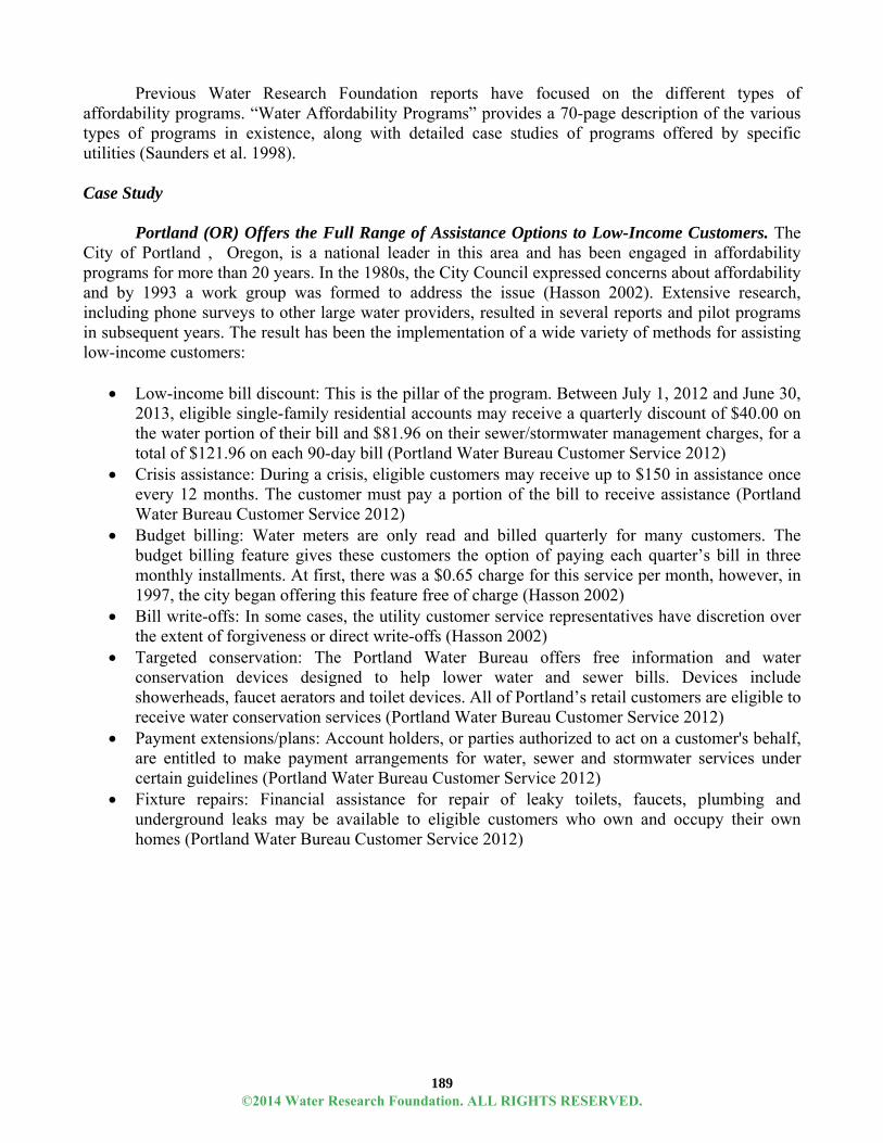
189
Previous Water Research Foundation reports have focused on the different types of affordability programs. “Water Affordability Programs” provides a 70-page description of the various types of programs in existence, along with detailed case studies of programs offered by specific utilities (Saunders et al. 1998). Case Study
Portland (OR) Offers the Full Range of Assistance Options to Low-Income Customers. The City of Portland , Oregon, is a national leader in this area and has been engaged in affordability programs for more than 20 years. In the 1980s, the City Council expressed concerns about affordability and by 1993 a work group was formed to address the issue (Hasson 2002). Extensive research, including phone surveys to other large water providers, resulted in several reports and pilot programs in subsequent years. The result has been the implementation of a wide variety of methods for assisting low-income customers:
Low-income bill discount: This is the pillar of the program. Between July 1, 2012 and June 30,
2013, eligible single-family residential accounts may receive a quarterly discount of $40.00 on the water portion of their bill and $81.96 on their sewer/stormwater management charges, for a total of $121.96 on each 90-day bill (Portland Water Bureau Customer Service 2012)
Crisis assistance: During a crisis, eligible customers may receive up to $150 in assistance once every 12 months. The customer must pay a portion of the bill to receive assistance (Portland Water Bureau Customer Service 2012)
Budget billing: Water meters are only read and billed quarterly for many customers. The budget billing feature gives these customers the option of paying each quarter’s bill in three monthly installments. At first, there was a $0.65 charge for this service per month, however, in 1997, the city began offering this feature free of charge (Hasson 2002)
Bill write-offs: In some cases, the utility customer service representatives have discretion over the extent of forgiveness or direct write-offs (Hasson 2002)
Targeted conservation: The Portland Water Bureau offers free information and water conservation devices designed to help lower water and sewer bills. Devices include showerheads, faucet aerators and toilet devices. All of Portland’s retail customers are eligible to receive water conservation services (Portland Water Bureau Customer Service 2012)
Payment extensions/plans: Account holders, or parties authorized to act on a customer's behalf, are entitled to make payment arrangements for water, sewer and stormwater services under certain guidelines (Portland Water Bureau Customer Service 2012)
Fixture repairs: Financial assistance for repair of leaky toilets, faucets, plumbing and underground leaks may be available to eligible customers who own and occupy their own homes (Portland Water Bureau Customer Service 2012)
©2014 Water Research Foundation. ALL RIGHTS RESERVED.

190
State Laws Influence the Design of Affordability Programs
At the federal level, the following statutory provision from the Clean Water Act (33 USC 1284(b)(1)) related to the federal requirement that utilities obtaining Clean Water State Revolving Funds money charge user fees (Clause A), acknowledges water affordability concerns:
“A system of user charges which imposes a lower charge for low-income residential users (as defined by the Administrator) shall be deemed to be a user charge system meeting the requirements of Clause (A) of this paragraph if the Administrator determines that such system was adopted after public notice and hearing.”
Federal law says little more on affordability programs, so it is largely up to the states to control such programs.
One of the newer areas of state law that affects affordability programs is California’s Proposition 218 and the related newer Proposition 26. These Propositions have led to a series of events where property owners and renters can reject water and sewer rate increases if more than 50% respond “in protest” to the increases. But, water utilities seem less concerned over this aspect of the law, describing it as more of a nuisance barrier. (In reality, even less than 50% of protest letters may be enough to have board members reconsider their decision to raise rates.) Perhaps more pressing is that one objective of the legislation is that rates are fair/equitable – discouraging one class of customer from subsidizing another. Article XIII, Section 6 of the California Constitution, states that “the amount of a fee or charge imposed upon any parcel or person as an incident of property ownership shall not exceed the proportional cost of the service attributable to the parcel.” This was added to State law on November 5, 1996 when California voters approved Proposition 218, “The Right to Vote on Taxes Act.” This raises more serious questions for affordability programs among California water utilities.
In some states, utilities are encouraged to use water rates revenue as the funding source for affordability programs. For example, in Pennsylvania, the Public Utility Commission (PUC) has provided for its Customer Assistance Programs (CAPs) that “cost recovery” will be handled as follows:
“Cost recovery. In evaluating utility CAPs for ratemaking purposes, the Commission will consider both revenue and expense impacts. Revenue impact considerations include a comparison between the amount of revenue collected from CAP participants prior to and during their enrollment in the CAP. CAP expense impacts include both the expenses associated with operating the CAPs as well as the potential decrease of customer utility operating expenses. Operating expenses include the return requirement on cash working capital for carrying arrearages, the cost of credit and collection activities for dealing with low income negative ability to pay customers, and uncollectible accounts expense for writing off bad debt for these customers.”
The PUC states that "program funding" should be derived from “operations and maintenance expense reductions." (CAP Policy Statement, at Section 69.265(1)) (Colton 2005).
In many other states, a utility’s rate revenues are restricted, or interpreted to be restricted, from being used to finance these types of assistance programs. North Carolina is one such state. In fact, in North Carolina, water utility revenues are not to be used to even administer these programs. Hence, a popular approach for North Carolina customer assistance programs has been for the water utility to partner with a local charity or human services organization to administer the program (Millonzi 2008). Millonzi interprets that law to mean that:
“Counties, cities, and public authorities all are prohibited from using utility proceeds to fund even the administration of an assistance program for utility customers. Counties and cities, however, have the option to appropriate general fund monies to fund such assistance programs for low or moderate income customers as well as senior citizens” (Millonzi 2012)
In Georgia, concerns exist over whether use of rates revenue is precluded due to restrictions on uses of public funds and/or bond covenant restrictions. The main issue has been whether funding an
©2014 Water Research Foundation. ALL RIGHTS RESERVED.
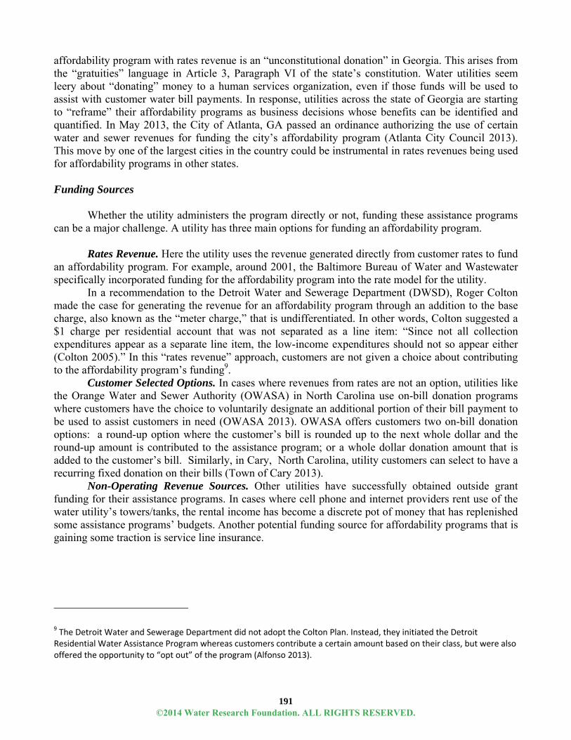
191
affordability program with rates revenue is an “unconstitutional donation” in Georgia. This arises from the “gratuities” language in Article 3, Paragraph VI of the state’s constitution. Water utilities seem leery about “donating” money to a human services organization, even if those funds will be used to assist with customer water bill payments. In response, utilities across the state of Georgia are starting to “reframe” their affordability programs as business decisions whose benefits can be identified and quantified. In May 2013, the City of Atlanta, GA passed an ordinance authorizing the use of certain water and sewer revenues for funding the city’s affordability program (Atlanta City Council 2013). This move by one of the largest cities in the country could be instrumental in rates revenues being used for affordability programs in other states. Funding Sources
Whether the utility administers the program directly or not, funding these assistance programs can be a major challenge. A utility has three main options for funding an affordability program.
Rates Revenue. Here the utility uses the revenue generated directly from customer rates to fund
an affordability program. For example, around 2001, the Baltimore Bureau of Water and Wastewater specifically incorporated funding for the affordability program into the rate model for the utility.
In a recommendation to the Detroit Water and Sewerage Department (DWSD), Roger Colton made the case for generating the revenue for an affordability program through an addition to the base charge, also known as the “meter charge,” that is undifferentiated. In other words, Colton suggested a $1 charge per residential account that was not separated as a line item: “Since not all collection expenditures appear as a separate line item, the low-income expenditures should not so appear either (Colton 2005).” In this “rates revenue” approach, customers are not given a choice about contributing to the affordability program’s funding9.
Customer Selected Options. In cases where revenues from rates are not an option, utilities like the Orange Water and Sewer Authority (OWASA) in North Carolina use on-bill donation programs where customers have the choice to voluntarily designate an additional portion of their bill payment to be used to assist customers in need (OWASA 2013). OWASA offers customers two on-bill donation options: a round-up option where the customer’s bill is rounded up to the next whole dollar and the round-up amount is contributed to the assistance program; or a whole dollar donation amount that is added to the customer’s bill. Similarly, in Cary, North Carolina, utility customers can select to have a recurring fixed donation on their bills (Town of Cary 2013).
Non-Operating Revenue Sources. Other utilities have successfully obtained outside grant funding for their assistance programs. In cases where cell phone and internet providers rent use of the water utility’s towers/tanks, the rental income has become a discrete pot of money that has replenished some assistance programs’ budgets. Another potential funding source for affordability programs that is gaining some traction is service line insurance.
9 The Detroit Water and Sewerage Department did not adopt the Colton Plan. Instead, they initiated the Detroit Residential Water Assistance Program whereas customers contribute a certain amount based on their class, but were also offered the opportunity to “opt out” of the program (Alfonso 2013).
©2014 Water Research Foundation. ALL RIGHTS RESERVED.
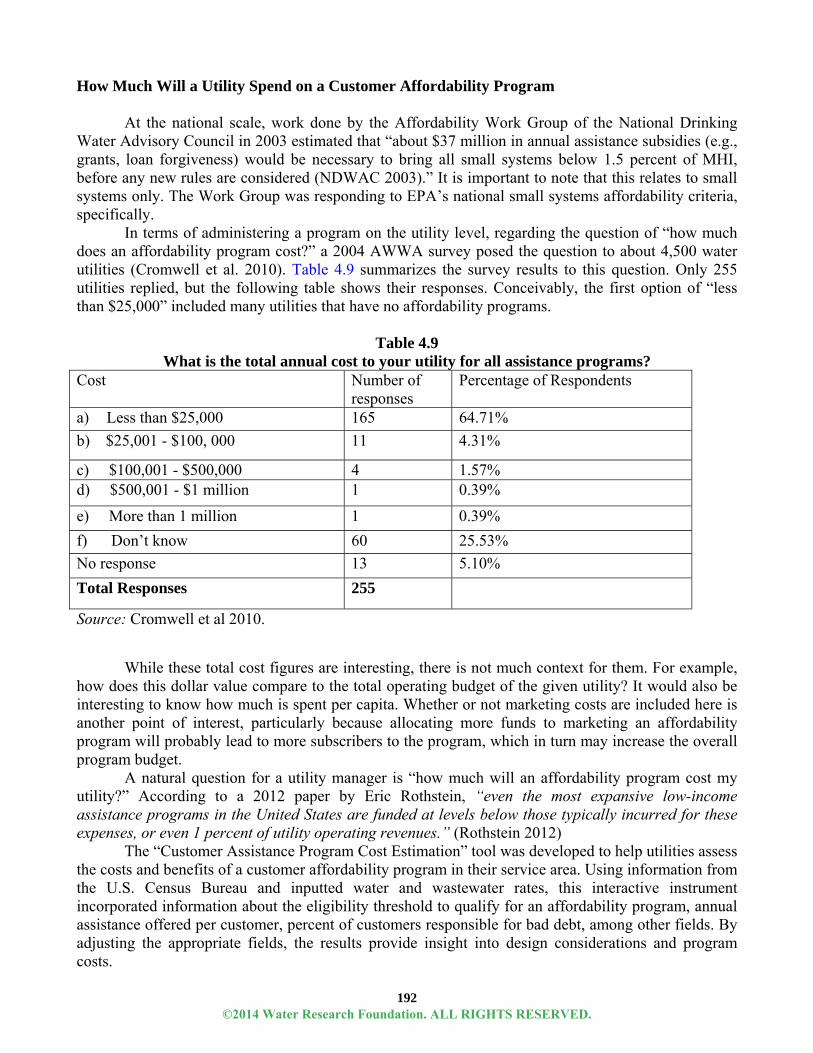
192
How Much Will a Utility Spend on a Customer Affordability Program
At the national scale, work done by the Affordability Work Group of the National Drinking Water Advisory Council in 2003 estimated that “about $37 million in annual assistance subsidies (e.g., grants, loan forgiveness) would be necessary to bring all small systems below 1.5 percent of MHI, before any new rules are considered (NDWAC 2003).” It is important to note that this relates to small systems only. The Work Group was responding to EPA’s national small systems affordability criteria, specifically.
In terms of administering a program on the utility level, regarding the question of “how much does an affordability program cost?” a 2004 AWWA survey posed the question to about 4,500 water utilities (Cromwell et al. 2010). Table 4.9 summarizes the survey results to this question. Only 255 utilities replied, but the following table shows their responses. Conceivably, the first option of “less than $25,000” included many utilities that have no affordability programs.
Table 4.9
What is the total annual cost to your utility for all assistance programs? Cost Number of
responses Percentage of Respondents
a) Less than $25,000 165 64.71%
b) $25,001 - $100, 000 11 4.31%
c) $100,001 - $500,000 4 1.57% d) $500,001 - $1 million 1 0.39%
e) More than 1 million 1 0.39%
f) Don’t know 60 25.53%
No response 13 5.10%
Total Responses 255
Source: Cromwell et al 2010.
While these total cost figures are interesting, there is not much context for them. For example,
how does this dollar value compare to the total operating budget of the given utility? It would also be interesting to know how much is spent per capita. Whether or not marketing costs are included here is another point of interest, particularly because allocating more funds to marketing an affordability program will probably lead to more subscribers to the program, which in turn may increase the overall program budget.
A natural question for a utility manager is “how much will an affordability program cost my utility?” According to a 2012 paper by Eric Rothstein, “even the most expansive low-income assistance programs in the United States are funded at levels below those typically incurred for these expenses, or even 1 percent of utility operating revenues.” (Rothstein 2012)
The “Customer Assistance Program Cost Estimation” tool was developed to help utilities assess the costs and benefits of a customer affordability program in their service area. Using information from the U.S. Census Bureau and inputted water and wastewater rates, this interactive instrument incorporated information about the eligibility threshold to qualify for an affordability program, annual assistance offered per customer, percent of customers responsible for bad debt, among other fields. By adjusting the appropriate fields, the results provide insight into design considerations and program costs.
©2014 Water Research Foundation. ALL RIGHTS RESERVED.

193
The tool was designed on the assumption that customers in need can access a fund a certain number of times per year to help them pay utility bills when necessary. The utility can adjust eligibility criteria and the amount of customer assistance per customer in a given year to determine direct program costs. It is built using Census information. An example of a summary for a given utility is:
"If a residential customer annually spends more than "2%" of their household income on “4 kgal"/month, they are eligible to receive up to “$125" in direct assistance per year assuming that they pay the rest of their bills. Only “50%” of eligible customers are expected to participate." (Items in quotation marks were inputs to the tool.)
Table 4.10 illustrates the differences in costs of a similarly constructed customer affordability program in three hypothetical systems inspired by three of the project’s utility partners. System characteristics, operating revenues, rate structures, and other tool inputs were adapted and incorporated into this analysis for comparison purposes. In order to show how an affordability program can affect utility systems of different characteristics, the analysis used common assumptions across all three systems: that in order to qualify for an assistance program offering $125 per eligible customer, households would have to spend 2% of their annual income on water and wastewater bill at 4 kgal/month.
Table 4.10 Customer affordability program details in three hypothetical water systems
System Characteristics System 1 System 2 System 3 Population 620,000 235,000 65,000 Median Household Income $40,000 $47,000 $115,000 Poverty Rate 22% 19% 3% 2011 Water and Wastewater Operating Revenues $290,000,000 $75,000,000 $25,000,000
Customer Affordability Tool Inputs A household is eligible if (x%) of its annual income
2%
is spent annually on water and wastewater bills at (x) kgal/month
4
Annual assistance amount per eligible account: $125 Estimate percent of eligible customers that will participate:
50%
Annual water and wastewater household charges for customers billed at 4 kgal/month: $441.36 $533.64 $368.52
(continued)
©2014 Water Research Foundation. ALL RIGHTS RESERVED.
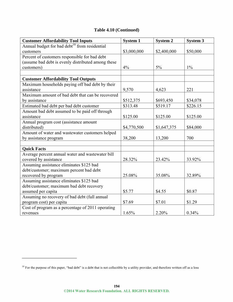
194
Table 4.10 (Continued)
Customer Affordability Tool Inputs System 1 System 2 System 3 Annual budget for bad debt10 from residential customers $3,000,000 $2,400,000 $50,000 Percent of customers responsible for bad debt (assume bad debt is evenly distributed among these customers) 4% 5% 1%
Customer Affordability Tool Outputs Maximum households paying off bad debt by their assistance 9,570 4,623 221 Maximum amount of bad debt that can be recovered by assistance $512,375 $693,450 $34,078 Estimated bad debt per bad debt customer $313.48 $519.17 $226.15 Amount bad debt assumed to be paid off through assistance $125.00 $125.00 $125.00 Annual program cost (assistance amount distributed) $4,770,500 $1,647,375 $84,000 Amount of water and wastewater customers helped by assistance program 38,200 13,200 700
Quick Facts Average percent annual water and wastewater bill covered by assistance 28.32% 23.42% 33.92% Assuming assistance eliminates $125 bad debt/customer; maximum percent bad debt recovered by program 25.08% 35.08% 32.89% Assuming assistance eliminates $125 bad debt/customer; maximum bad debt recovery assumed per capita $5.77 $4.55 $0.87 Assuming no recovery of bad debt (full annual program cost) per capita $7.69 $7.01 $1.29 Cost of program as a percentage of 2011 operating revenues 1.65% 2.20% 0.34%
10 For the purpose of this paper, “bad debt” is a debt that is not collectible by a utility provider, and therefore written off as a loss
©2014 Water Research Foundation. ALL RIGHTS RESERVED.

195
Holding for these same assumptions across all towns, the affordability tool analysis provides interesting insights into how MHI, poverty rate, and population can affect the costs per capita of running such a program, among other takeaways. This information helps in understanding why an affordability program may cost more in System 1 than in System 3.
As seen above, for System 3 to run an affordability program using the provided background information, the cost would range from $0.87 to $1.29 per capita annually. That is, the average individual would see a maximum total annual increase of $1.29 on their utility bill, with the chance that there would only be an increase of $0.87 per person if the system is successful in collecting the maximum amount of bad debt through assistance. This scenario will not occur for all utilities, by observing the effects of an assistance program on the other two systems, customers would see an average annual increase ranging from $4.55 to $7.69 per capita.
It should come as no surprise that an assistance program in Systems 1 and 2 costs more than in System 3 when observing how the different characteristics determine the number of households that qualify for assistance. For example, System 3 has a MHI of nearly three times as much as System 1, and a poverty rate over seven times smaller than System 1, which leads to approximately 6% of the total population in System 1 to qualifying for assistance, while approximately 1% of the total population in System 3 qualifies. Given these findings, such a program still has minimal negative financial effects on each of the three utility systems in the analysis, as it represents approximately 0.3 to 2.2% of their operating revenues. While these findings may be limited to three cases, they illustrate Eric Rothstein’s conclusion that implementing an assistance program is relatively affordable for most systems. (Rothstein 2012)
Impact of Customer Affordability on Utility Operations
That non-payment due to affordability issues affects a water utility’s bottom line is not
disputed. Since dealing with late payments, service disconnects/reconnects, and uncollectible accounts (bad debt) is very costly relative to the amount of money involved, a low-income assistance program can potentially provide significant savings to the utility by reducing those costs. However, it is difficult to quantify the costs and benefits of affordability programs in the water industry. For example, work done to recommend an affordability program to Detroit states that while “(a) low-income affordability program can reasonably be expected to generate expense savings that will offset, at least in part, the cost of the revenue loss attributable to the proposed rate discount, … due to the unavailability of data, those offsets cannot be calculated for the DWSD program (Colton 2005).”
Owing to this lack of literature in the water sector, research focused on another utility sector to garner what has been done on quantifying the financial benefits of an affordability program. Research published from the electricity industry does seem to offer some relevant analogies. Customer Assistance in the Energy Sector
In Oregon, there is a heavy energy burden on low-income customers, where such customers typically spend 16% of annual income on energy, compared with 5% for other households (Elliott 2006). A study conducted by Quantec LLC in 2003 found that the societal benefits derived from the Oregon Low- Income Weatherization program slightly exceeded the costs, while the benefits to the utilities as measured through cost savings were slightly less than the program costs. The study itemized utility costs as follows:
1) Reductions in past due amounts of $340 per customer 2) Savings of $11 per participant due to the time value of money and reduced need to acquire
capital
©2014 Water Research Foundation. ALL RIGHTS RESERVED.

196
3) Reduction of $190,000 in costs related to efforts to collect bad debt (including phone calls, letters, customer visits, and collection agency costs)
4) Reduction in customer mobility caused by need to move due to high energy costs resulted in estimated cost savings to utility of $22,000 related to reading meter prior to assigning new account; and
5) Possible increase in federal assistance from Low Income Home Energy Assistance Program (LIHEAP) attributable to state-sponsored program.
Additionally, the writers observe that certain benefits of the Oregon program could not be
quantified, and concluded that if those factors were taken into consideration, the program’s cost effectiveness would have increased significantly (Khawaja and Baggett 2003).
The approach analyzed the affordability program costs and benefits from the perspective of two energy utilities - PacifiCorp and PGE; as well as that of the State of Oregon in general (societal). In calculating Benefit-Cost (B/C) Ratios, a B/C ratio of 1.0 is the “breakeven point” where what the utility receives back in benefit is just equal to the investment. Values above 1.0 indicate “profitable investments.” The results showed the Oregon energy affordability program to be cost effective from the state-level (societal) perspective with benefit/cost ratio 1.03. From the utility perspective, the Program is slightly short of cost effectiveness with a B/C ratio of 0.96 (Khawaja and Baggett 2003).
Why Low Income Customers Perhaps Should Pay Less?
In general, low-income electricity customers have been described as having “flatter-than average load profiles (Wood and Faruqui 2010).” If this is assumed to be true for water customers as well, it lends to the business case for charging low-income customers less since they contribute less to system peaking.
Apart from their usage patterns, low-income customers may be at risk of facing a disproportionate share of water utility costs, unless the utility adjusts the base/fixed charge. This is because, as average per capita water use continues to decline, the charge per unit of consumption will increase in order to cover the fixed costs of the water utility. Low-income customers will lack the ability to change out toilets, washing machines, and other hardware with water-saving appliances. Therefore, these underprivileged customers will bear an increased burden of covering the fixed costs of the water utility. Meanwhile, as prices rise, more customers will find it in their financial interest to invest in water efficiency – further increasing the burden on low-income customers.
From a more holistic or qualitative viewpoint, research on energy customer assistance programs found that such programs “provide utility staff persons greater satisfaction in their jobs (Fisher, Sheehan and Colton 2010).” The fact that a utility was offering assistance to low-income customers is also looked upon favorably by the community and affords the utility “reputational capital” as explained by Fisher, Sheenan and Colton (2010). These authors go further to point out that “because rate affordability programs contribute to additional disposable income within the low-income population, it helps drive additional job creation, income generation, and economic activity for local businesses (Fisher, Sheehan and Colton 2010).” Low-income households tend to be comprised of hourly-paid workers. The case has been made that the lost work hours involved in setting-up utility reconnection further exacerbates the income problem for these customers.
As a way to maximize limited resources, customer assistance programs can be argued to allow a utility to re-direct its “bill collections” and “disconnections” line items towards customers who do not have the ability to pay (Colton 2007). The idea here is that these utility funds/activities have less useful impact on low-income customers than they have on wealthier customers (Colton 2007).
By avoiding disconnection and mitigating accruals of past due balances, both the utility and the customer may benefit financially from affordability programs. From the utility’s perspective,
©2014 Water Research Foundation. ALL RIGHTS RESERVED.

197
“maintaining customer service billings effectively provides the system with an annuity whose value becomes substantial as customer retention persists over time (Rothstein 2012).” As an example, with the City of Atlanta’s “Care and Conserve” assistance program which provides up to $500 of assistance every three years, if one assumes that the typical participating household’s water and sewer bill is $50 per month, Rothstein points out that retention of a customer for less than one additional year would achieve positive cash flow. Admittedly, not all program participants would be disconnected except for the provision of assistance; and not all those whose disconnection is forestalled will remain customers for even an additional year. However, many will be benefitted in this way, and some will remain customers for extended periods, each providing the type of financial returns explained above.
Many of the financial benefits mentioned thus far have been indirect benefits, but even direct benefits are difficult to quantify. The following case study from the City of Baltimore, MD illustrates this utility’s attempt to quantify the finances of its water customer assistance program. Case Study
Baltimore Bureau of Water and Wastewater. Like many older US cities with combined sewers, the Baltimore Bureau of Water and Wastewater faces a consent decree. In response, the City is proactively negotiating to ramp up its remedial efforts to address discharge and overflow issues. The cost of the construction and maintenance are estimated to be more than $1 billion dollars over the next two decades. The City has committed to financing these remedial efforts through a combination of water and waste water revenue bonds in conjunction with all available State and Federal assistance (City of Baltimore 2011) and has been raising water and wastewater rates by approximately 9% each year since 2003 in order to generate the revenue to cover these bonds. Figure 4.17 below shows the change in Baltimore’s quarterly base and volumetric charge for block one (all consumption between 10 ccf and 50 ccf per quarter).
Figure 4.17 Change in Baltimore City’s charges for residential water
While rate increases are seldom popular, the scenario of a consent decree provides utility decision-makers with some measure of political cover. However, affordability issues within Baltimore’s service population prompted the City to develop a two-pronged customer assistance approach in response to the cost of the consent decree.
$0
$2
$4
$6
$8
$10
$12
2002 2003 2004 2005 2006 2007 2008 2009 2010 2011 2012
YearBaseChargePerQuarter(includes10ccfpermeter) RatePerCCFforFirst50ccf
©2014 Water Research Foundation. ALL RIGHTS RESERVED.
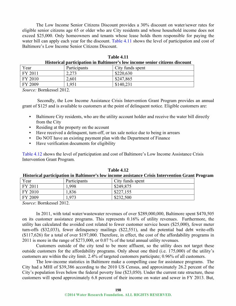
198
The Low Income Senior Citizens Discount provides a 30% discount on water/sewer rates for eligible senior citizens age 65 or older who are City residents and whose household income does not exceed $25,000. Only homeowners and tenants whose lease holds them responsible for paying the water bill can apply each year for the discount. Table 4.11 shows the level of participation and cost of Baltimore’s Low Income Senior Citizens Discount.
Table 4.11
Historical participation in Baltimore’s low income senior citizens discount Year Participants City funds spent FY 2011 2,273 $220,630 FY 2010 2,601 $247,865 FY 2009 1,951 $140,231 Source: Bornkessel 2012.
Secondly, the Low Income Assistance Crisis Intervention Grant Program provides an annual grant of $125 and is available to customers at the point of delinquent notice. Eligible customers are:
• Baltimore City residents, who are the utility account holder and receive the water bill directly
from the City • Residing at the property on the account • Have received a delinquent, turn-off, or tax sale notice due to being in arrears • Do NOT have an existing payment plan with the Department of Finance • Have verification documents for eligibility
Table 4.12 shows the level of participation and cost of Baltimore’s Low Income Assistance Crisis Intervention Grant Program.
Table 4.12 Historical participation in Baltimore’s low income assistance Crisis Intervention Grant Program Year Participants City funds spent FY 2011 1,998 $249,875 FY 2010 1,836 $227,155 FY 2009 1,973 $232,500 Source: Bornkessel 2012.
In 2011, with total water/wastewater revenues of over $289,000,000, Baltimore spent $470,505 on its customer assistance programs. This represents 0.16% of utility revenues. Furthermore, the utility has calculated the avoided cost related to fewer customer service hours ($25,000), fewer meter turn-offs ($32,033), fewer delinquency mailings ($22,551), and the potential bad debt write-offs ($117,626) for a total of over $197,000. Therefore, in effect, the cost of the affordability programs in 2011 is more in the range of $273,000, or 0.07 % of the total annual utility revenues.
Customers outside of the city tend to be more affluent, so the utility does not target these outside customers for the affordability programs. Only about one third (i.e. 175,000) of the utility’s customers are within the city limit. 2.4% of targeted customers participate; 0.96% of all customers.
The low-income statistics in Baltimore make a compelling case for assistance programs. The City had a MHI of $39,386 according to the 2010 US Census, and approximately 26.2 percent of the City’s population lives below the federal poverty line ($23,050). Under the current rate structure, these customers will spend approximately 6.8 percent of their income on water and sewer in FY 2013. But,
©2014 Water Research Foundation. ALL RIGHTS RESERVED.

199
of that 26.2 percent, 12.3 percent of the City’s population lives below half of the federal poverty line, indicating that while the City-wide MHI is $39,386, a large percentage of customers have significantly lower income levels. Conclusions This section explored some of the financial constructs and reasoning behind customer affordability programs. Methods for generating the revenue to fund these types of programs, depending on the limitations of state law, were also considered. While the financial or business case for implementing an affordability program was explored, the research did not pinpoint the larger indirect financial benefits of customer affordability programs for water utilities. Clearly, keeping rates unsustainably low for everyone at the cost of water and wastewater infrastructure investment benefits no one in the long term. Affordability programs provide flexibility to utilities seeking revenue resiliency. References Alfonso, Mary. 2013. Email exchange regarding affordability program. September 23, 2013. Association of California Water Agencies. 2012. AB 685 headed to the Governor’s Desk – Your Veto
Request Letters are Needed! [Online]. Available: <http://outreach.acwa.com/site/MessageViewer?em_id=3521.0> [cited December 22, 2012]
Atlanta City Council. 2013. Ordinance 13-0-0119. Approved May 15, 2013. Atlanta, Ga.: City of Atlanta.
AWWA (American Water Works Association). 2012a. Buried No Longer: Confronting America’s Water Infrastructure Challenge. Denver, Colo.: AWWA.
AWWA (American Water Works Association). 2012b. M1 Manual: Principles of Water Rates, Fees, and Charges. Denver, Colo.: AWWA.
Bornkessel, B. 2012. < [email protected]> e-mail message to author, S. Berahzer. <[email protected]>.
California General Assembly. 2012. Bill No. 685, An act to add Section 106.3 to the Water Code, relating to water. Sacramento. [Online]. Available: <http://www.leginfo.ca.gov/pub/11-12/bill/asm/ab_0651-0700/ab_685_bill_20120925_chaptered.pdf>. [cited December 22, 2012]
City of Baltimore. 2011. 2011 Comprehensive Annual Financial Report. Baltimore, Md.: City of Baltimore.
Colton, R. 2005. A Water Affordability Program for Detroit Water and Sewerage Department (DWSD). Belmont, Mass.: Fisher, Sheehan & Colton.
Colton, R. 2007. The Impact of Indiana’s Low-Income Affordability Programs on Nonpayment Disconnections. Belmont, Mass.: Fisher, Sheehan, & Colton.
Cromwell, J.E., R. Colton, S. Rubin, C. Herrick, J. Mobley, K. Reinhardt, and R. Wilson. 2010. Best Practices in Customer Assistance Programs. Denver, Colo.: Water Research Foundation.
EFAB (Environmental Financial Advisory Board). 2006. Affordable Rate Design for Households. Atlanta, Ga.: EFAB.
EFAB (Environmental Financial Advisory Board). 2007. Comments on EPA Document: Combined Sewer Overflows—Guidance for Financial Capability Assessment and Schedule Development. Atlanta, Ga.: EFAB. [Online]. Available: <http://www.efc.unc.edu/publications/2011/Financial_Capacity_Review_Report.pdf>. [cited January 2, 2013]
Elliott, D. Low Income Weatherization – Current Successes and Future Directions. Presented at Poverty Conference, Portland, Ore., October 2006.) [Online]. Available:
©2014 Water Research Foundation. ALL RIGHTS RESERVED.

200
<http://www.oregon.gov/ohcs/CRD/SOS/docs/Pov_Conf_06_Wx_Pres_Final.pdf>. [cited January 2, 2013]
Fisher, Sheehan and Colton. Utility Rate Affordability: The Indirect Business Benefits. FSC’s Law & Economic Insights, 10(6):1-6. [Online]. Available: http://www.fsconline.com/downloads/FSC%20Newsletter/news2010/n2010_1112.pdf [cited January 2, 2013]
Hasson, D. 2002. Water Utility Options for Low-Income Assistance Programs. Jour. AWWA, 94(4): 138.
Hayward, K. 2011. The Human Right to Water and Sanitation: The View of the UN’s Independent Expert. Water 21 Magazine of the International Water Association, October.
Khawaja, S and S. Baggett. 2003. Final Report: Oregon Energy Assistance Program Evaluation. Prepared for Oregon Housing and Community Services. Portland, Ore.: Quantec, LLC.
Millonzi, K. 2008. Guide to Billing and Collecting Public Enterprise Utility Fees for Water, Wastewater, and Solid Waste Services. Chapel Hill, N.C.: University of North Carolina School of Government.
Millonzi, K. 2012. May 31 (10:22 a.m.). comment on Stacey Isaac Berahzer, The Increasing Need to Address Customer Affordability. The Environmental Finance Center Blog. May 29, 2012. [Online]. Available: <https://efc.web.unc.edu/2012/05/29/the-increasing-need-to-address-customer-affordability/ > [cited May 1, 2013]
Mumm, J. 2012. Money Matters: Accepting the Affordability Challenge. Jour. AWWA, 104(5): 27-28. NACWA (National Association of Clean Water Agencies). 2005. Financial Capability and
Affordability in Wet Weather Negotiations. Washington D.C.: CH2M HILL. [Online]. Available: <http://www.nacwa.org/index.php?option=com_content&view=article&id=476%3A2005-nacwa-financialcapability-and-affordability-in-wet-weather-negotiations-white-paper&catid=8%3Apublications&Itemid=7> [cited May 9, 2013]
NACWA (National Association of Clean Water Agencies). 2007. Principles for Assessment and Negotiation of Financial Capability: A Compilation of Resources. Washington D.C.: CH2M HILL. [Online]. Available: <http://www.nacwa.org/index.php?option=com_content&view=article&id=1636&Itemid=271> [cited May 9, 2013]
NDWAC (National Drinking Water Advisory Council). 2003. Recommendations of the National Drinking Water Advisory Council to U.S. EPA on its National Small Systems Affordability Criteria. Washington D.C.: NDWAC.
OWASA (Orange Water and Sewer Authority). 2009. Resolution Adopting Orange Water and Sewer Authority Financial Management Policy. Adopted March 26, 2009. N.C.: OWASA.
OWASA (Orange Water and Sewer Authority). Taste of Hope. [Online]. Available: <http://www.owasa.org/customerService/taste-of-hope.aspx>. [cited January 3, 2013]
Portland Water Bureau Customer Service. 2012. Need help paying your water and sewer bill? Portland, Ore.: City of Portland, Oregon. [Online]. Available:
<http://www.portlandoregon.gov/water/article/371216> [cited January 2, 2013] Rothstein, E. 2012.The Business Case for Low-Income Affordability Programs. Proceedings of the
2012 Utility Management Conference, Miami, Fla., January 30-February 2: Water Environment Federation.
Saunders, Kimmel, Spade, and Brockway. 1998. Water Affordability Programs – Project 184 1998. Denver, Colo.: AwwaRF.
Town of Cary (North Carolina). Department of Finance: Oasis. [Online]. Available: <http://www.townofcary.org/Departments/Finance/Utility_Accounts/Oasis.htm>. [cited on January 3, 2013]
©2014 Water Research Foundation. ALL RIGHTS RESERVED.

201
United Nations General Assembly. 2010. Resolution 64/292 The Human Right to Water and Sanitation. Adopted July 28, 2010. [Online]. Available: <http://www.un.org/ga/search/view_doc.asp?symbol=A/RES/64/292> [cited on December 12, 2012]
USEPA (United States Environmental Protection Agency). 2009. 2009 Drinking Water Infrastructure Needs Survey and Assessment: Fourth Report to Congress. Washington, D.C.: USEPA.
Wood, L and A. Faruqui. 2010. Dynamic Pricing and Low-Income Customers: correcting misconceptions about load-management programs. Public Utilities Fortnightly, 148(11): 60. [Online] Available: <http://www.edisonfoundation.net/IEE/Documents/PUF_11-01-2010_Final_LowIncome.pdf> [cited January 2, 2013].
RATE ADJUSTMENT APPROACHES
Introduction
Revenue resiliency necessitates water rates that are sufficient to keep up with the rising costs of
managing water resources and running a utility. Rate increases should happen “slowly, but surely.” The Chapter 2 section on Trends in Rates and Pricing showed the relationship between the degree of rate increases and financial performance. In theory, most government-owned utilities would like to follow a pricing approach that is directly linked to their revenue requirements. As service sales and revenue requirements evolve, managers would be able to quickly and expediently modify rates accordingly. This “cost-of-service approach is promoted across the industry and is in place in many utilities (AWWA 2012), however this process is hindered in many situations by political pressure, non-cost oriented pricing objectives, and regulatory requirements. Facing a governing board to get its approval for rate increases is usually one of the least appealing parts of a water utility manager’s job. While, some governing bodies have the experience to see the importance of frequent, incremental rate increases, it seems this is the exception. Water utility pricing cannot always be separated from other pressing social and governmental challenges. For example, some governing boards responsible for general government functions and utility services may subjectively balance the increase of water rates with increases on general fund taxes and charges. So in a year when taxes rise, water rates may stagnate. Furthermore, if the board member hopes to serve a subsequent term, such prospects are usually not brightened by having voted to increase the water rate. There is a tremendous amount of evidence showing that current water and sewer prices are far from adequate in meeting existing revenue requirements, so it is not surprising that many utility managers have looked to “less than perfect” pricing practices to increase the resiliency of their business.
©2014 Water Research Foundation. ALL RIGHTS RESERVED.

202
Figure 4.18 Alternative rate adjustment approaches can help water utility managers ensure a level of rate increases, despite political challenges
This section examines automatic pricing adjustments that do not rely solely on revenue requirements. Having a process in place where rates increase “automatically,” without having to go to a decision-making body annually for approval, obviously has some appeal to utility managers. The process of automatic rate increases helps to mitigate some of the financial risk associated with political uncertainty; however it could lead to other types of financial risk. Three alternative methods of approach rate adjustments are discussed below; each has potential drawbacks that a utility should consider. These potential hurdles are considered in the individual sections that follow. Key Points
Revenues are a function of sales and pricing. Sales are difficult to predict, and pricing is difficult to modify for many utilities. Under this backdrop, some utilities may benefit from adopting a process for “automatically” adjusting rates for a multi-year period instead of relying on a one-time cost justified rate adjustment request.
Alternative approaches to rate adjustments, including pass through clauses, indexed rate adjustments, and multi-year rate adjustment plans, have advantages and disadvantages that have to be clearly evaluated at the utility level before adopting this practice.
Cost-Indexed Rate Adjustments To keep up with increasing costs due to inflation, additional regulatory requirements, and the
need to repair or replace aging infrastructure, some utilities have begun to rely on indexed rate increases to help boost the revenue stream without requiring annual approval of rate increases by the governing body. With indexed rates, a utility’s governing body approves annual rate increases based on a specified cost index, such as the Consumer Price Index (CPI) for a certain period of time. In theory, this approach allows the utility’s revenue to increase without the governing body having to approve increases each year.
©2014 Water Research Foundation. ALL RIGHTS RESERVED.

203
The Case for Indexed Rates
The cost of providing water and sewer service is generally increasing. The three largest operation and maintenance (O&M) costs for water and wastewater utilities are labor, power, and chemicals. While the amount of power and chemical used is directly influenced by the amount of water a utility sells, labor is not. Utility labor costs generally do not fluctuate based on the amount of water sold. A utility needs to maintain its staff, even if water sales were down one month. In response to the recession, many utilities eliminated or reduced cost-of-living adjustments to salaries. However, this can be considered a temporary adjustment, and salary increases are expected in the longer term. Historically, along with these cost-of-living adjustments, utilities have also had merit increases. So, employees’ positions have been at a higher pay rate and employees have moved up within the wage scale. The escalating health care costs liability have seriously impacted the benefits component of labor costs. Power and chemical costs have also seen fluctuations, with significant increases at certain times. Therefore, the cost of these three largest components of O&M costs increase every year, even though the same level of service remains the same.
In addition to O&M increases, capital costs have also been increasing. Utilities have had capital expenditures necessary to gain compliance with new regulatory requirements. Many utilities have also begun to ramp up spending on repair and replacement of aging infrastructure. These trends are likely to continue.
Another advantage of indexed rates is that they may be positively received by groups that tend to be critical of government, since the use of indexed rates forces a utility to manage within a certain revenue stream. From the perspective of critics of governmental utilities, this prevents the utility from simply increasing rates to pay for costs that are unnecessarily increased.
As more utilities are recognizing the need and benefit of annual increases, utilities are looking for approaches that do not require going in front of the governing body to approve every rate increase. For political reasons, providing an option where governing bodies can somewhat distance themselves from increases can be viewed positively by the members of the body. Indexed rates are one solution. Limitations of Indexed Rates
One of the risks of indexed rates is that the escalation factor afforded by the index selected may
not capture all of the revenue needs of a utility. Utility management, and more importantly governing bodies, may be lured into a false sense of financial security. It may be more difficult to gain approval for additional increases in later years if the public has been convinced that indexed rate increases would be sufficient. For example, additional regulatory requirements may result in revenue needs increasing more significantly than expected, which could cause a shortfall from indexed rate increases. Also, declines in demand, which many utilities are currently experiencing, could cause financial challenges for utilities that rely solely on indexed rates. Furthermore, this report’s assessment of Trends in Pricing and Rates showed that the majority of utilities surveyed in the AWWA-RFC Water and Wastewater Rate Surveys increased rates much faster, on average, than the Consumer Price Index, as it did in many states. This suggests that cost-indexed rates may be of little or even negative benefit to utilities economic recessions and depressions.
As with all practices, utilities will have to take into consideration their unique circumstances when evaluating the appropriateness of automatic pricing adjustments. Certainly a utility that is about to embark on a major capital project that will result in a dramatic increase in costs will not see prices adjusted by inflation as a resiliency strategy, but a utility with a fairly stable cost outlook and stable customer base may have a very different perspective.
©2014 Water Research Foundation. ALL RIGHTS RESERVED.
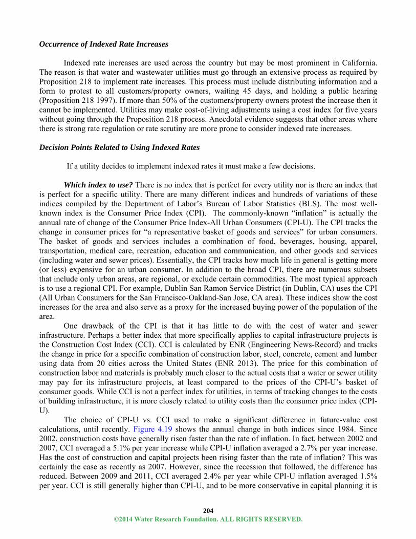
204
Occurrence of Indexed Rate Increases
Indexed rate increases are used across the country but may be most prominent in California. The reason is that water and wastewater utilities must go through an extensive process as required by Proposition 218 to implement rate increases. This process must include distributing information and a form to protest to all customers/property owners, waiting 45 days, and holding a public hearing (Proposition 218 1997). If more than 50% of the customers/property owners protest the increase then it cannot be implemented. Utilities may make cost-of-living adjustments using a cost index for five years without going through the Proposition 218 process. Anecdotal evidence suggests that other areas where there is strong rate regulation or rate scrutiny are more prone to consider indexed rate increases. Decision Points Related to Using Indexed Rates
If a utility decides to implement indexed rates it must make a few decisions. Which index to use? There is no index that is perfect for every utility nor is there an index that
is perfect for a specific utility. There are many different indices and hundreds of variations of these indices compiled by the Department of Labor’s Bureau of Labor Statistics (BLS). The most well-known index is the Consumer Price Index (CPI). The commonly-known “inflation” is actually the annual rate of change of the Consumer Price Index-All Urban Consumers (CPI-U). The CPI tracks the change in consumer prices for “a representative basket of goods and services” for urban consumers. The basket of goods and services includes a combination of food, beverages, housing, apparel, transportation, medical care, recreation, education and communication, and other goods and services (including water and sewer prices). Essentially, the CPI tracks how much life in general is getting more (or less) expensive for an urban consumer. In addition to the broad CPI, there are numerous subsets that include only urban areas, are regional, or exclude certain commodities. The most typical approach is to use a regional CPI. For example, Dublin San Ramon Service District (in Dublin, CA) uses the CPI (All Urban Consumers for the San Francisco-Oakland-San Jose, CA area). These indices show the cost increases for the area and also serve as a proxy for the increased buying power of the population of the area.
One drawback of the CPI is that it has little to do with the cost of water and sewer infrastructure. Perhaps a better index that more specifically applies to capital infrastructure projects is the Construction Cost Index (CCI). CCI is calculated by ENR (Engineering News-Record) and tracks the change in price for a specific combination of construction labor, steel, concrete, cement and lumber using data from 20 cities across the United States (ENR 2013). The price for this combination of construction labor and materials is probably much closer to the actual costs that a water or sewer utility may pay for its infrastructure projects, at least compared to the prices of the CPI-U’s basket of consumer goods. While CCI is not a perfect index for utilities, in terms of tracking changes to the costs of building infrastructure, it is more closely related to utility costs than the consumer price index (CPI-U).
The choice of CPI-U vs. CCI used to make a significant difference in future-value cost calculations, until recently. Figure 4.19 shows the annual change in both indices since 1984. Since 2002, construction costs have generally risen faster than the rate of inflation. In fact, between 2002 and 2007, CCI averaged a 5.1% per year increase while CPI-U inflation averaged a 2.7% per year increase. Has the cost of construction and capital projects been rising faster than the rate of inflation? This was certainly the case as recently as 2007. However, since the recession that followed, the difference has reduced. Between 2009 and 2011, CCI averaged 2.4% per year while CPI-U inflation averaged 1.5% per year. CCI is still generally higher than CPI-U, and to be more conservative in capital planning it is
©2014 Water Research Foundation. ALL RIGHTS RESERVED.

205
wise for utilities to use the higher inflation rate in order to better prepare for possible increases to construction costs.
Figure 4.19 Annual changes to CPI-U (“inflation”) and CCI: 1984- 2012
As a word of caution, from 2008 to 2012, both CPI-U and CCI fluctuated. Predicting what will happen to these indices is difficult, but by using a graph such as this one, a utility can make informed decisions about which index to use for financial decisions such as rate setting.
Many utilities will turn to customized indexes that are prepared by professional associations or regional entities. For example, in Griffin, Georgia, the utility tags its water rates to the Municipal Cost Index (MCI). This index is produced by “American City and County” and has been around since 1978 (American City and County 2013).
The BLS also tracks the “water and sewer maintenance index,” which may also be useful in comparing rate increases. The “water and sewerage maintenance” index, tracks changes to the seasonally-adjusted water/sewer monthly bill that is charged to households in 87 urban communities, and it is not the change of costs of maintenance that utilities face to repair, rehabilitate or replace infrastructure11.
Which periods to use? For the indices provided by the BLS, updates are usually available
monthly. However, there is some lag between the end of the month and when the index is released; there are often slight adjustments to the previous period(s). Therefore, a utility should choose three or
11 http://www.inflationsummary.com/ConsumerPriceIndex/Housing/FuelsandUtilities/WaterandSewerandTrashCollectionServices/WaterandSewerageMaintenance
©2014 Water Research Foundation. ALL RIGHTS RESERVED.

206
four months in advance to compare from year to year. For example, if a utility wants to have annual increases on July 1, it should not try to use the June over June change in the index. Instead, it should select March over March or February over February. Therefore, a utility that uses CPI may compare the February 2012 CPI to the February 2011 CPI to calculate the increase to become effective July 1, 2012.
How to handle unexpected events? The utility also must have a plan for addressing unexpected
events. Over time, most indices have averaged annual increases of 2% to 3%. However, due to the recession, most indices actually fell between some months in 2008 and 2009. If the utility is committed to using the index, it might be required to lower rates at this time. Due to the recession and other factors, many utilities were experiencing declines in water usage at the same time. The combination of these factors could result in a significant decline in revenue
Combining Performance Incentives with Rate Indexing
Another critique of pure cost indexing is that it could take away the incentive for efficiency. EPCOR Water Services Inc., a private utility with public roots that serves Edmonton, Canada has a pricing adjustment process (see case study box), incorporates performance measurement and efficiency drivers into their system.
Case Study
EPCOR Water Services Inc. EPCOR Water Services Inc. (EPCOR) is a private company which operates the water system according to Performance Based Regulations (PBR) found in the City of Edmonton Waterworks Bylaw. There is a general process for increasing rates, but, included therein is the fact that if the utility is not able to achieve a certain level of performance in a given year, then it must rebate its customers in the subsequent year (City of Edmonton 2012).
EPCOR considers the performance approach to provide the benefits of:
1. Assuring customers that their utility must meet performance standards 2. Ensuring customers receive stable and predictable rates over the five year period (there is a
five year rate filing with annual progress reports reducing the amount of materials to be produced annually)
3. Protecting customers from unexpected rate increases, as EWSI (EPCOR) bears the risk of greater than expected cost increases
4. Encouraging EWSI (EPCOR) to keep costs low and to find more innovative and efficient ways to improve the operations of its system Of course, other factors besides performance are considered. Figure 4.20 was taken from the
PBR Progress Report for 2011, and illustrates how the various components of the PBR conceptual framework inter-relate.
©2014 Water Research Foundation. ALL RIGHTS RESERVED.

207
Figure 4.20 This conceptual framework shows the various areas that are considered in deciding on the level of the water rate. 2011 Performance Measures – Water System Service Quality Standards
Target Points Actual Points Earned Actual Outcome
System Reliability Index 25.0 27.5 Exceeded target
Water Quality Index 25.0 25.0 Met target
Customer Service Index 20.0 21.6 Exceeded target
Environmental Index 15.0 14.5 Below target
Safety Index 15.0 16.3 Exceeded target
Aggregate Points Earned (sum of all indicies)
100.0 104.9
Figure 4.21 Honing in on the performance of the utility, scores are available in five 5 different categories for a total of 100. (Exceeding the target levels in some areas resulted in a score of over 100 in this case. However, there is no reward to the utility for scoring higher than 100.)
Figure 4.21 shows the scoring mechanism for individual performance measures in 2011. According to the Bylaws, for each full point scored below 100 base and bonus points, a penalty of $67,000 will be assessed to a maximum of $1,000,000. The total penalty for the year is applied as a rebate to customers in the year immediately following the performance year (City of Edmonton 2012).
©2014 Water Research Foundation. ALL RIGHTS RESERVED.

208
Like most utilities, EPCOR does compare its rates to other cities and local communities, in an attempt to make sure that its rates are reasonable and competitive. But, unlike most other utilities, EPCOR faces financial penalties if performance measures are not met. The method of calculating the overall rate increase is outlined below. Once this rate is calculated, the performance penalty is subtracted from the fixed rate portion of the water bill.
According to the 2011 PBR Progress Report, the bulk of the rate increase is calculated by the following process:
“Under the PBR framework for 2007-2011, water rate increases are based on inflation, less a 0.25% efficiency factor. For PBR purposes, inflation is weighted 79% on Alberta CPI and 21% on labor inflation (based on the annual percentage increase negotiated and accepted by the bargaining units representing EPCOR’s unionized employees within the City).” For all 5 years of the 2007 – 2011 PBR term, EPCOR exceeded the operating performance
standards, achieving 104.9 points compared to the PBR standard of 100 points. So, performance has not hampered the utility’s financial model recently.
For 2011, this whole process meant that water consumption charges increased by 1.36% over the 2010 levels1213. Summary
Indexed rates have potential benefits to some utilities. In general, they provide rate increases
(and revenue increases) without the challenges of getting rates annually approved. However, indexed rates are not without their limitations. Utilities using indexed rates should develop policies that provide for decreases in the index, and indexed rate increases that fall short of the revenue needs of the utility. The initial discussions that lead to the adoption of indexed rates should include these caveats, and frame this process as only one part of the rate setting and revenue forecasting toolbox of a utility. Multi-year Rate Increases
Here the term “multiyear rate increase” refers to a utility gaining approval for a series of
increases that spans several years. This is included under this section of “automatic” rate increases, despite the fact that the first year of this type of rate increase probably feels anything but automatic and often does incorporate a cost justification in a staged rate adjustment plan. This process at least prevents the utility manager from standing in front of the governing body with “hat in hand” every single year (as shown in Figure 4.18).
12 This increase consists of the 2011 forecast inflation factor of 2.05%, minus a 2010 actual-to-forecast inflation factor adjustment of 0.69%. (The 0.69% was based on 2010 forecast inflation of 2.44% to actual 2010 inflation of 1.75%). 13 2 other non-routine adjustments (NRAs) were approved for 2011: Accelerated Water Main Renewal (AWMR) – “The annual increase from the AWMR program resulted in a $0.35 per meter per month increase to the monthly fixed charges based on a 15 mm equivalent meter size (standard household meter size).”An increase in franchise rate in response to the 2009 increase in franchise fee by City Council
©2014 Water Research Foundation. ALL RIGHTS RESERVED.

209
Multiyear Rate Increases in Public Water Utilities There are different variations to the use of a multi-year rate adjustment approach. Some utilities
have financial plans and rate models that are vetted and provisionally approved by governing boards for use in subsequent years without knowing the exact future rate increases. In other situations, some public utilities have convinced their boards to approve multi-year increases based on a financial plan done in a particular year. Such was the case in December 2012 when the City Council in New Orleans’ approved a rate increase of 10% for the following eight years (Rainey 2012). After undergoing a rate study that lasted more than two and a half years, the Sewerage & Water Board of New Orleans gained approval of a proposed program of rate increases that will raise a typical customers’ monthly. Undoubtedly, part of what made the process so controversial and protracted for New Orleans is the stigmatized “doubling of rates within eight years”. But, this idea of approving a series of increases at one time is certainly not novel in the industry. The following three examples from this project’s partner utilities serve as a proxy for the occurrence of this practice in the industry.
One of the most common practices is to carry out a rate analysis and to project estimated rate needs for a multi-year period. These increases are cost based, but get “frozen” in time at the time of approval and often do not take into consideration changes in demand or other sales assumptions in out years. For example, Gwinnett County, GA with its “2009 Water and Sewer Rate Resolution” was able to institute a series of rate increases in one shot described in Figure 4.22 below.
Figure 4.22 Approved increases to Gwinnet County Water’s volumetric charges set forth in its 2009 Water and Sewer Rate Resolution (Gwinnett County 2009).
Similarly, Mesa Consolidated Water District in California passed Resolution 1384 which approved rate increases from 2010 to 2014 shown in Figure 4.23.
Commodity Charges for Potable, Recycled, Construction, and Fireline Water, Basic Charges, and LAFCO Surcharges Effective for water used on and after January 1, 2010
Usage Charge Per Unit* (CCF):
FY2010 FY2011 FY2012 FY2013 FY2014
Potable $2.60 $2.70 $2.85 $3.00 $3.15 Recycled $2.34 $2.43 $2.57 $2.70 $2.84 Construction $3.90 $4.05 $4.28 $4.50 $4.73 Fire $5.20 $5.40 $5.70 $6.00 $6.30 *One unit equals 100 cubic feet or 748 gallons Figure 4.23 Mesa Consolidated Water District rate schedule from 2010 to 2014
©2014 Water Research Foundation. ALL RIGHTS RESERVED.
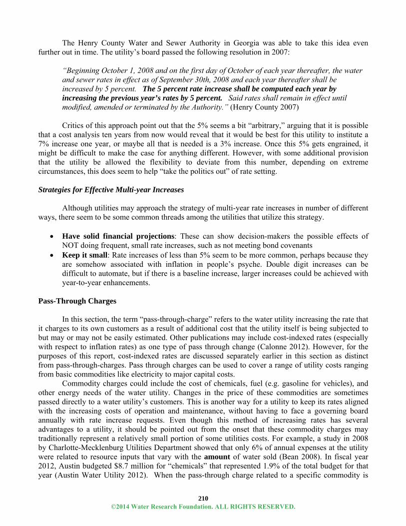
210
The Henry County Water and Sewer Authority in Georgia was able to take this idea even further out in time. The utility’s board passed the following resolution in 2007:
“Beginning October 1, 2008 and on the first day of October of each year thereafter, the water and sewer rates in effect as of September 30th, 2008 and each year thereafter shall be increased by 5 percent. The 5 percent rate increase shall be computed each year by increasing the previous year’s rates by 5 percent. Said rates shall remain in effect until modified, amended or terminated by the Authority.” (Henry County 2007) Critics of this approach point out that the 5% seems a bit “arbitrary,” arguing that it is possible
that a cost analysis ten years from now would reveal that it would be best for this utility to institute a 7% increase one year, or maybe all that is needed is a 3% increase. Once this 5% gets engrained, it might be difficult to make the case for anything different. However, with some additional provision that the utility be allowed the flexibility to deviate from this number, depending on extreme circumstances, this does seem to help “take the politics out” of rate setting.
Strategies for Effective Multi-year Increases
Although utilities may approach the strategy of multi-year rate increases in number of different
ways, there seem to be some common threads among the utilities that utilize this strategy.
Have solid financial projections: These can show decision-makers the possible effects of NOT doing frequent, small rate increases, such as not meeting bond covenants
Keep it small: Rate increases of less than 5% seem to be more common, perhaps because they are somehow associated with inflation in people’s psyche. Double digit increases can be difficult to automate, but if there is a baseline increase, larger increases could be achieved with year-to-year enhancements.
Pass-Through Charges
In this section, the term “pass-through-charge” refers to the water utility increasing the rate that
it charges to its own customers as a result of additional cost that the utility itself is being subjected to but may or may not be easily estimated. Other publications may include cost-indexed rates (especially with respect to inflation rates) as one type of pass through change (Calonne 2012). However, for the purposes of this report, cost-indexed rates are discussed separately earlier in this section as distinct from pass-through-charges. Pass through charges can be used to cover a range of utility costs ranging from basic commodities like electricity to major capital costs.
Commodity charges could include the cost of chemicals, fuel (e.g. gasoline for vehicles), and other energy needs of the water utility. Changes in the price of these commodities are sometimes passed directly to a water utility’s customers. This is another way for a utility to keep its rates aligned with the increasing costs of operation and maintenance, without having to face a governing board annually with rate increase requests. Even though this method of increasing rates has several advantages to a utility, it should be pointed out from the onset that these commodity charges may traditionally represent a relatively small portion of some utilities costs. For example, a study in 2008 by Charlotte-Mecklenburg Utilities Department showed that only 6% of annual expenses at the utility were related to resource inputs that vary with the amount of water sold (Bean 2008). In fiscal year 2012, Austin budgeted $8.7 million for “chemicals” that represented 1.9% of the total budget for that year (Austin Water Utility 2012). When the pass-through charge related to a specific commodity is
©2014 Water Research Foundation. ALL RIGHTS RESERVED.

211
such a small fraction of a utility’s expenses, it needs to be clear to decision-makers that the pass-through charge is just one small way of keeping up with the rising costs of utility operation, and other rate adjustment methods need to be in place.
In some cases a utility purchases its water from another utility and then re-sells that water to its own customers. In this case of a purchase water system, the largest “commodity” would be the actual water purchased: raw or treated. This is certainly not a small portion of the utility’s budget, and pass-through charges have more significance for purchase water systems. For example, during periods of high use, the City of Tampa Bay purchases water from Tampa Bay Water. The City uses a pass-through charge to its own customers. A per unit cost is calculated from the total cost for all of the purchases from Tampa Bay Water during the previous three month period. The amount each customer pays is calculated by multiplying their individual usage times that per unit cost. The surcharge appears a separate line item on the utility bill (City of Tampa Bay 2007).
In California, Government Code Section 53756 authorizes agencies to adopt a schedule of fees or charges authorizing automatic adjustments that pass through increases in wholesale charges for water and adjustments for inflation for a period of five (5) years (Proposition 218 1997). For example, “Resolution 641-10, adopted by the Monte Vista Water District Board of Directors in January 2010, established a three-year schedule of water rates and also authorized, as provided by state law, the ability to “pass through” to customers any increases in wholesale water service charges which exceed, in any fiscal year, the amount of scheduled increase in the adopted rates.” (Monte Vista Water District 2013)
Similarly, in Orange, CA, the utility buys water from two different providers14. The City of Orange has adopted the following pass-through formula: Pass-through charge = [Revised Supply Cost)*(Revised Water Supplied) – (Plan Supply Cost)*(Planned Water Supplied)]
Where: Revised Supply Cost = cost of water based on provided water purveyor rates, basin pumping percentage for the current year, and electricity costs Revise Water Supplied = water consumption for current year Plan Supply Cost = estimated cost of water based on provided water purveyor rates, basin pumping percentage at the time of the rate study, and electricity costs Planned Water Supplied = estimated water demand at the time of the rate study
The “revised water supplied” has the additional advantage that it appears to allow this utility to decouple rates from consumption.
In Southern California, scarce water supplies have resulted in some expensive capital projects. The $1 billion Carlsbad Desalination Project, for example, was approved in 2012 and is expected to be completed in 2016. Another project was the $1.5 billion Emergency Storage Project by the San Diego County Water Authority (SDCWA). Olivenhain Municipal Water District (OMWD) purchases all of its water from SDCWA. As a result of the emergency storage project, OMWD looked at a 7.5% increase to its own customers (OMWD 2013). In order to explain these rate increases to its customers,
14 These providers are the Orange County Water District (OCWD) and the Metropolitan Water District of Southern California (MET).
©2014 Water Research Foundation. ALL RIGHTS RESERVED.

212
OMWD included Figure 4.24 in a newsletter to its customers (Shandling 2013).
Figure 4.24 OMWD Increases in Rates and Charges vs. SDCWA Increases and San Diego CPI: Image from Olivenhain Municipal Water District’s Newsletter Highlighting Pass- Through-Charges (OMWD 2013)
While many pass-through charges are linked to third-party charges imparted on the utility, the City of Alamo Heights, TX, adopted an ordinance in July 2012 that authorizes pass through charges for funding a Habitat Conservation Plan. Alamo Heights draws water from the Edwards Aquifer. In recent decades, demand for water has outstripped the aquifer's capacity to provide at past levels. There are increasing concerns about the welfare of endangered species and regional economies that depend on spring flows from the aquifer. The pass-through-charge will be used by the Edwards Aquifer Authority to fund amelioration of habitat destruction (City of Alamo Heights 2012).
Investor owned utilities typically follow a different economic regulatory framework that influences their ability to implement pricing practices (See Section on Economic Regulation). The use of indexing, multi-year rates, and pass-through charges varies from state to state, but in some cases has become quite prevalent particularly in the area of creating pass-through charges. For example, there is some evidence that the “method of choice” that is emerging in the private water sector is the distribution system improvement charge (DSIC) model that Pennsylvania pioneered in 1997. DSIC allows a utility to bundle a set of infrastructure improvement projects together and collect the needed funds from rate payers in a variation of a pass-through charge. This “bundling” saves the time and costs involved in making several individual rate cases. Several other states, including New York, Connecticut, and Delaware have followed suit with programs similar to DSIC (American Water Intelligence 2012). Programs like DSIC allow the company to avoid borrowing for certain projects. Instead, the company can recover the costs, through rates, almost simultaneously to performing the infrastructure project. So, in essence, the company gets approved for rate increases for a set of projects, instead of a set of years.
In another example, the private water utility, EPCOR Water Services Inc., serves the City of Edmonton in Canada and is required to pay a “franchise fee” to the city. According to the “Waterworks
©2014 Water Research Foundation. ALL RIGHTS RESERVED.

213
Bylaw” EPCOR is permitted to have a “non-routine adjustment” in rates to EPCOR customers. Therefore, as a result of a 0.4% increase in the franchise fee that went into effect on April 1, 2010, there was a $0.13 per meter per month increase to the monthly fixed charged based on a 15mm equivalent meter size (EPCOR 2012).).
Observations From the Energy Sector
In the energy sector, requests for other types of surcharges and tracking mechanisms by utilities
have significantly increased recently. In fact, in 2012, the National Regulatory Research Institute characterized the use of cost trackers and mechanisms as the “latest trend.” The Institute defined trackers as automatic adjustments to rates and trackers are approved in rate cases for specific future events, durations, and amounts. Trackers allow utilities to recover (or rebate) between rate cases the adjustments prospectively approved in the rate case. But experts in the energy field warn that the increasing imposition of surcharges and other alternative ratemaking mechanisms can also defeat some of the primary principles of the rate-setting and regulatory review process (Larkin & Associates 2012).
Costello (2009) provides “Seven Major Points” from the energy sector that relate to pass-through-charges that could have relevance to water utilities as well:
1. There has been a proliferation of “cost trackers” in recent years, covering the gamut of utility
functions and activities 2. Regulators generally have approved these new charges for a wide array of utility functions 3. Regulators in recent years have applied less stringent criteria for the approval of cost trackers 4. Regulators have given inadequate attention to the negative features of cost trackers. By
conflicting with certain regulatory objectives, cost trackers are at odds with the public interest 5. A rate-of-return tracker in the form of an earnings sharing mechanism has advantages over
having myriad trackers for a single utility 6. Regulators should consider traditional regulation as the default policy unless a utility is able to
demonstrate that it needs a cost tracker to prevent the possibility of a serious financial condition, and
7. Regulators should attach conditions to cost trackers
Some of these points may appear less relevant where water charges are not regulated by entities such as public service commissions, however, elected officials who make decisions on water rates would do well to pay attention to these concerns from some experts in the energy industry.
©2014 Water Research Foundation. ALL RIGHTS RESERVED.

214
Conclusion This section provided a variety of approaches to raising water rates that involve a process
besides approaching a decision-making board every year with annual cost justified rate modification requests. Cost-indexed rates, multi-year increases, and pass-through charges all involve an initial decision by the governing body, but that decision would have long term effect on utility revenue. These processes for raising rates incrementally help quell some of political and public adversity to rate increases. But, another important financial side-benefit to annual rate increases (as opposed to increases every few years) relates to the power of compounding.
References American City & County. 2013. Municipal Cost Index Archive. [Online]. Available:
<http://americancityandcounty.com/municipal-cost-index/2013> [cited May 14, 2013] American Water Intelligence. 2012. PaPUC Shows Brotherly Love for Private Water Companies.
American Water Intelligence, 3(8). [Online]. Available: <http://www.americanwaterintel.com/archive/3/8/profile/papuc-shows-brotherly-love-private-water-companies.html> [cited on May 24, 2013]
Austin Water Utility. 2012. FY2012 Approved Budget: Fixed and Variable Costs. Austin, Tex.: Austin Water Utility.
(AWWA) American Water Works Association. 2012. M1: Principle of Water Rates, Fees and Charges, 6th ed. Denver: Colo.: AWWA
Bean, D. 2008. Revenue Expenses for Charlotte-Mecklenburg Utilities in a Given Year. Presented at Charlotte City Council Meeting, Charlotte, N.C., December 1, 2008.
Calonne, A.P. 2012. City of Ventura – City Attorney Legal Report, July 9. Ventura, Calif.: City of Ventura.
City of Alamo Heights. 2012. Ordinance 1933. Alamo Heights, Tex.: City Council of the City of Alamo Heights. [Online]. Available: <http://www.alamoheightstx.gov/government/documents/Ord1933AmendingChpt.19HCPPlan.pdf> [cited February 28, 2012]
City of Edmonton. 2012. EPCOR Water Services and Wastewater Treatment Bylaw. Edmonton (Alberta), Canada: The City of Edmonton. [Online]. Available: <http://www.edmonton.ca/bylaws_licences/C15816.pdf > [cited April 22, 2013]
City of Tampa. 2007. Resolution No 2007-631, A Resolution to Include a Specific Formula to Calculate the Cost of Potable Water Purchased from Tampa Bay Water to be Charged to City of Tampa Water Customers. [Online]. Available: <http://www.tampagov.net/dept_water/files/Resolutions_and_Ordinances/TBW_Passthrough_Resolution_2007-631.pdf> [cited April 24, 2013]
Costello, K. 2009. Talking Points on Cost Trackers. Presented before the NARUC (National Association of Regulatory Utility Commissioners), Chicago Ill. November 15 and 1, 2009.
Engineering News Record. 2013 (copyright year). Using ENR Indexes. [Online]. Available: <http://enr.construction.com/economics/FAQ.asp> [cited April 12, 2013]
EPCOR Water Services Inc. 2012. 2007 – 2011 Performance Based Regulation. Edmonton (Alberta), Canada: EPCOR Water Services.
Gwinnett County. 2009. Water and Sewer Rate Resolution. [Online]. Available: <http://www.gwinnettcounty.com/static/departments/publicutilities/pdf/waterrateresolution.pdf> [cited May 9, 2013]
Henry County. 2007. Resolution No. 2007-20. Adopted September 25, 2007. Henry County, Ga.: Henry County Water and Sewerage Authority.
©2014 Water Research Foundation. ALL RIGHTS RESERVED.

215
Larkin & Associates. 2012. Increasing Use of Surcharges on Consumer Utility Bills – for the AARP. Surprise, Ariz.: Larkin & Associates. [Online]. Available: <http://www.aarp.org/content/dam/aarp/aarp_foundation/2012-06/increasing-use-of-surcharges-on-consumer-utility-bills-aarp.pdf > [cited May 9, 2013]
Monte Vista Water District. 2013. Notice of “Pass Through” Water Charges. Montclair, Calif.: Monte Vista Water District. [Online]. Available: <http://www.mvwd.org/download.cfm?ID=544> [cited April 24, 2013].
OMWD (Olivenhain Municipal Water District). 2013. Watching Water – Your District News, February. Encitas, Calif.: OMWD. [Online]. Available: <http://www.olivenhain.com/files/docs/publications/newsletters/2013/Feb2013WW.pdf> [cited May 9, 2013]
Proposition 218. 1997. California Government Code § 53756. [Online]. Available: <http://codes.lp.findlaw.com/cacode/GOV/1/5/d2/1/4/4.6/s53756#sthash.0TQCSBxJ.dpuf> [cited on February 28, 2013]
Rainey, R. 2012. New Orleans City Council passes major sewer and water rate hikes. The Times-Picayune, December 6. New Orleans, La. [Online]. Available: <http://www.nola.com/politics/index.ssf/2012/12/new_orleans_city_council_passe_4.html> [cited May 24, 2013]
Shandling, K. 2013. Water and the Fiscal Cliff. Water Utility Infrastructure Management, February. [Online]. Available: < http://www.uimonline.com/index/webapp-stories-action/id.865/archive.yes/Issue.2013-02-01/title.water-&-the-fiscal-cliff> [cited May 9, 2013]
©2014 Water Research Foundation. ALL RIGHTS RESERVED.

©2014 Water Research Foundation. ALL RIGHTS RESERVED.
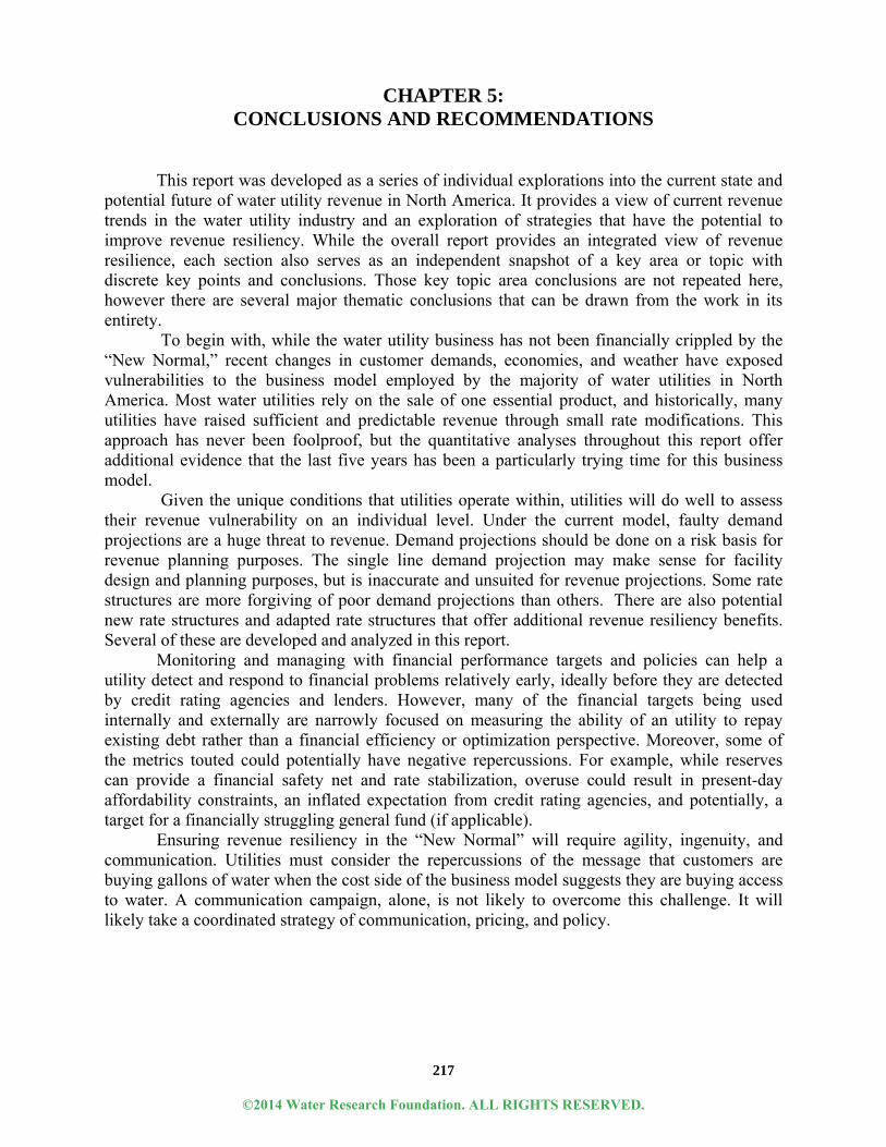
217
CHAPTER 5: CONCLUSIONS AND RECOMMENDATIONS
This report was developed as a series of individual explorations into the current state and potential future of water utility revenue in North America. It provides a view of current revenue trends in the water utility industry and an exploration of strategies that have the potential to improve revenue resiliency. While the overall report provides an integrated view of revenue resilience, each section also serves as an independent snapshot of a key area or topic with discrete key points and conclusions. Those key topic area conclusions are not repeated here, however there are several major thematic conclusions that can be drawn from the work in its entirety.
To begin with, while the water utility business has not been financially crippled by the “New Normal,” recent changes in customer demands, economies, and weather have exposed vulnerabilities to the business model employed by the majority of water utilities in North America. Most water utilities rely on the sale of one essential product, and historically, many utilities have raised sufficient and predictable revenue through small rate modifications. This approach has never been foolproof, but the quantitative analyses throughout this report offer additional evidence that the last five years has been a particularly trying time for this business model.
Given the unique conditions that utilities operate within, utilities will do well to assess their revenue vulnerability on an individual level. Under the current model, faulty demand projections are a huge threat to revenue. Demand projections should be done on a risk basis for revenue planning purposes. The single line demand projection may make sense for facility design and planning purposes, but is inaccurate and unsuited for revenue projections. Some rate structures are more forgiving of poor demand projections than others. There are also potential new rate structures and adapted rate structures that offer additional revenue resiliency benefits. Several of these are developed and analyzed in this report.
Monitoring and managing with financial performance targets and policies can help a utility detect and respond to financial problems relatively early, ideally before they are detected by credit rating agencies and lenders. However, many of the financial targets being used internally and externally are narrowly focused on measuring the ability of an utility to repay existing debt rather than a financial efficiency or optimization perspective. Moreover, some of the metrics touted could potentially have negative repercussions. For example, while reserves can provide a financial safety net and rate stabilization, overuse could result in present-day affordability constraints, an inflated expectation from credit rating agencies, and potentially, a target for a financially struggling general fund (if applicable).
Ensuring revenue resiliency in the “New Normal” will require agility, ingenuity, and communication. Utilities must consider the repercussions of the message that customers are buying gallons of water when the cost side of the business model suggests they are buying access to water. A communication campaign, alone, is not likely to overcome this challenge. It will likely take a coordinated strategy of communication, pricing, and policy.
©2014 Water Research Foundation. ALL RIGHTS RESERVED.

©2014 Water Research Foundation. ALL RIGHTS RESERVED.

219
ABBREVIATIONS
ACWD Alameda County Water District ADS annual debt service AJC Atlanta Journal Constitution (Newspaper) AMI Advanced Metering Infrastructure ASCE American Society of Civil Engineers avg. Average AWMR Accelerated Water Main Renewal AWWA American Water Works Association AWWA-RFC American Water Works Association-Raftelis Financial Consultants B/C Benefit-Cost BJWSA Beaufort-Jasper Water and Sewer Authority BLS Department of Labor’s Bureau of Labor Statistics CAFR Comprehensive Annual Financial Reports CAP Customer Assistance Program CCI Construction Cost Index CIP Capital Improvement Plans ccf 100 cubic feet CMUD Charlotte-Mecklenburg Utility Department Corp. Corporation CPI Consumer Price Index CPI-U Consumer Price Index-All Urban Consumers CSO Combined Sewer Overflows CUWCC California Urban Water Conservation Council CWRPDA Colorado Water Resources and Power Development Authority DC Water District of Columbia Water and Sewer Authority DSIC distribution system improvement charge model from Pennsylvania DWSD Detroit Water and Sewerage Department D0 drought, abnormally dry D1 drought conditions, moderate D2 drought conditions, severe D3 drought conditions, extreme D4 drought conditions, exceptional ed. edition EFAB Environmental Advisory Board EFC Environmental Finance Center at the University of North Carolina e.g. exempli gratia (for the sake of example) ENR Engineering News-Record EPA US Environmental Protection Agency EPCOR EPCOR Water Services Inc. ERU Equivalent Residential Unit et al. and others etc. etcetera
©2014 Water Research Foundation. ALL RIGHTS RESERVED.

220
EUM Effective Utility Management EWSI EPCOR Water Services Inc. FY Fiscal Year gal gallon GEFA Georgia Environmental Finance Authority GFOA Government Finance Officers Association HB House Bill hholds households HRWC Halifax Regional Water Commission HRM Halifax Regional Municipality i.e. id est (that is) Inc. Incorporated kgal one thousand gallons kGPM one thousand gallons per month LAFCO Orange County Local Agency Formation Commission LGC Local Government Commission LIHEAP Low Income Home Energy Assistance Program LWSP Local Water Supply Plans MADS maximum annual debt service max. maximum MCEQ Mississippi Commission on Environmental Quality MCI Municipal Cost Index MET Metropolitan Water District of Southern California MGD millions of gallons per day MHI Median Household Income mm millimeter MNGWPD Metropolitan North Georgia Water Planning District MWD Metropolitan Water District of Southern California n number NA Not Applicable NACWA National Association of Clean Water Agencies NBC National Broadcasting Company NCDENR North Carolina Department of Environment and Natural Resources NCLM North Carolina League of Municipalities NDWAC National Drinking Water Advisory Council No. Number NRA non-routine adjustments NRRI National Regulatory Research Institute OCWD Orange County Water District OFWAT Office of Water
©2014 Water Research Foundation. ALL RIGHTS RESERVED.

221
OH EPA Ohio Environmental Protection Agency O&M Operations and Maintenance OMWD Olivenhain Municipal Water District OWASA Orange Water and Sewer Authority OWDA Ohio Water Development Agency PAY-GO Pay as you go PBR Performance Based Regulations Prop Proposition PSC Public Service Commission of WI PUC Public Utility Commission of Pennsylvania R&R Repair and Rehabilitation RFC Raftelis Financial Consultants, Inc. RSE Rate Stabilization and Equalization SDCWA San Diego County Water Authority S&P Standard and Poor’s SPU Seattle Public Utilities TML Texas Municipal League TQM Total Quality Management TWDB Texas Water Development Board UN United Nations USDA United States Department of Agriculture USEPA United States Environmental Protection Agency V Volumetric Rates WI PSC Wisconsin Public Service Commission
©2014 Water Research Foundation. ALL RIGHTS RESERVED.

©2014 Water Research Foundation. ALL RIGHTS RESERVED.

223
ADDENDUMS
A FINANCIAL POLICY STRAWMAN
Financial policies represent an important element in the long-term plan of a utility because they help to ensure the financial sustainability of the organization. These policies often consist of a set of financial targets and provide direction and guidance for how governing bodies should proceed in certain situations. Financial policies often include statements that address the utility’s stance on topics including but not limited to: credit, debt, operations, reserves, and rates. The following details the indicators that are often used to assess the overall health and long-term sustainability of a utility organization.
Also included is a best practices strawman for water utility financial metrics, which will be referred to in each of the metric sections. The Strawman presents possible targets for each financial policy. These targets were identified based on data provided by the project’s utility partners experience working with utilities across the country. It is critical that utilities adjust these targets to fit their current situations. For example, it is of little value for a utility to have a target such as parity coverage of 2.0x that is only attainable through extraordinarily high rate increases or to have a target that the utility can easily exceed even without improved financial performance. Once a set of financial policies are put into place, these policies should be reviewed on at least an annual or bi-annual basis to determine whether adjustments are necessary.
Financial Metric Policy Target
Debt Service Coverage Ratio Parity coverage of 1.5x Total coverage of 1.2x
Debt Load Debt service less than 40% of total revenue requirements
Capital Funding Minimum of 25% of annual capital expenses funded
through rate-funded capital (PAYGO)
Days Cash on Hand 180 days O&M Budget Escalation Maximum annual O&M budget escalation of 5%
Operating Reserve Fund Minimum fund balance of 90 days of annual O&M expenses
Capital Reserve Fund Minimum fund balance of 25% of annual Capital expenses
Rate/Revenue Stabilization Fund (Demand Shortfall Fund)
Minimum fund balance target of 5% of projected annual revenues
Rate Revenue Composition Minimum of 25% of annual revenue from fixed charges
Rate Increases Minimum of automatic rate increases indexed to CPI
Service Affordability Maximum annual bill of an average customer of 2% of median household for each water and wastewater
©2014 Water Research Foundation. ALL RIGHTS RESERVED.

224
Credit Rating
Because it is a composite indicator with significant implications, one of the most important metrics for a utility is its credit rating. Assigned by one of the credit bureaus (Fitch, Moody’s, and Standard & Poor’s), the credit rating indicates the ability of the utility to meet its financial obligations in full in a timely manner. It is largely what determines the utility’s ability to borrow funds to finance capital projects on favorable terms. Utilities receive credit ratings from one or more rating agencies. Because so much information is required by the ratings agencies in determining a rating, the credit rating is generally the single encapsulating metric that best represents the overall financial health of the utility. It was not included in the previous table because it is a function of the financial policies and not under the direct control of the utility. Debt
The capital cost associated with the provision of water and wastewater service is
significant, and is thus most efficiently financed through debt. Though the credit rating helps to determine the terms on which debt will be issued, there are several other metrics associated with debt. Many utilities choose to implement specific policies regarding the debt service coverage ratio, the debt load, and/or the debt composition.
The debt service coverage ratio is a primary indicator of the financial health of a utility. It is a ratio of the revenues available for debt service to the cost of the debt service. The metric indicates a utility’s ability to produce enough cash to cover its debt obligations. If a utility has a debt service coverage ratio of less than 1.0x, this is likely an indication of a mismatch between revenues and revenue requirements, with the ratio indicating the inability of the utility to meet its obligations. Bond covenants typically require debt service coverage of anywhere between 1.00x and 1.30x. If a utility does not satisfy its covenant it may be required to initiate a rate study to avoid being considered in default even if it is making the necessary debt service payments. Because this is a basic and important metric, many utilities have financial policies that require total debt service coverage that is 10 to 20 basis points greater than their bond covenants. The 2013 Fitch Ratings Median Report for the Water and Sewer Industry found that the median All-In All Debt Service Coverage Ratio was 2.0x (Fitch 2013). The Strawman presents a potential total debt service coverage ratio target of 1.2x and a potential parity coverage ratio target of 1.5x. After reviewing the Strawman, one Utility Partner offered the following advice for utilities establishing their debt service coverage ratio targets, “Be careful not to set the target too high; our Board’s policy is 2.0x without system development charges, which has driven rate increases for many years and has not allowed us to leverage debt to minimize rates.” In general, meeting these targets should be achievable without being too easy for utilities. Debt load and debt composition are important secondary considerations regarding utility indebtedness. The debt load, which is the total amount of debt accumulated, can give insight into the system’s rates and its capacity for additional debt, in addition to providing a sense of whether the system is expanding or in the midst of a rehabilitation-focused capital program. The Strawman suggests a target of total debt service being less than 40% of total revenue requirements. The 2013 Fitch Ratings Median Report for the
©2014 Water Research Foundation. ALL RIGHTS RESERVED.

225
Water and Sewer Industry found that the median All-In Debt Service as % of Gross Revenues was 21% (Fitch 2013). The composition of the debt, which shows the mix of short- and long-term debt, is also significant, as it indicates how efficiently the utility is able to borrow funds. If a utility’s debt is largely variable rate, the instability may require the utility to direct resources to debt that may have been otherwise used to cover other costs. Financial policies around debt load and debt composition could include limiting the debt load as a percentage of the total revenue requirements and limiting the percent of debt that can be borrowed at a variable rate. A related measure, Capital Funding, indicates a utility’s ability to pay for capital projects with cash. This is an important financial metric for utilities to be aware of, as paying for capital projects using PAYGO (pay as you go) funds will be less expensive than financing exclusively through debt issuances. PAYGO financing helps minimize the reliance on debt-financing and improves a utility’s debt service coverage ratio. In this case, the Strawman suggests a minimum of 25% of annual capital expenditures funded directly through rates.
Operations
Much like the debt service coverage ratio is a basic indicator of cash flow, Days Cash on
Hand represents the ability of existing cash reserves to meet near-term obligations. It is calculated by dividing the total unrestricted reserves by the O&M budget and multiplying by 365. The combination of aging infrastructure and climate change could have significant short-term financial impacts on utilities. Cash reserves help weather the need for immediate, unexpected capital repairs (such as a pipeline break in a major transmission line) and events that could interrupt cash flow (such as a hurricane). As such, utilities need to maintain some level of unrestricted cash on hand as working capital to mitigate revenue shortfalls. Utilities are also subject to seasonal fluctuations, with revenue significantly impacted by the weather and climate, so cash reserves are important to ensure operational sustainability. Financial policies regarding the days of cash on hand typically include a minimum number of days’ worth of operating expenses. The 2013 Fitch Ratings Median Report for the Water and Sewer Industry found that the median Days Cash on Hand for all of the utilities it rated in 2012 was 417 days (Fitch 2013).
The O&M Budget Escalation metric is significant in that it represents the level of
efficiency that the utility has achieved. Utility service cannot always avoid the political realm. As such, and particularly when rate increases become necessary, it is important for utilities to be able to demonstrate that they have taken steps to ensure that their costs remain low. Financial policies regarding O&M budget escalation generally include a range of escalation that the utility must remain within. The Strawman presents a suggested policy target of a maximum escalation of 5%, which is one possible target. Because circumstances could occur that would require utilities to exceed their target escalations, exceeding this metric could trigger the utility to do a detailed review of the O&M budget.
©2014 Water Research Foundation. ALL RIGHTS RESERVED.

226
Reserves
Reserve funds help utilities fund expected and unexpected projects and protect utilities from disruptions in revenue streams. Most utilities have at least two reserve funds, one with restricted funds, which can be used only for designated purposes such as debt service, and one that has more flexible unrestricted funds. Within unrestricted reserves, utilities often have operating reserve funds, capital reserve funds, and/or rate/revenue stabilization funds. These reserve funds taken together are the basis for the Days Cash on Hand. In general, large unrestricted reserve funds are positive indicators of the health of the utility.
Financial policies associated with reserve funds tend to include setting a minimum fund balance as a percentage of expenses or revenues. Two common minimum targets are a percentage of specific expenses or of projected operating revenues. An Operating Reserve Fund helps utilities to weather unexpected short-term revenue shortages, expenses, or losses. This type of fund provides a back stop if the utility is unable to collect revenues for a certain period of time (one example would be if billing systems were to fail for an extended period of time due to a severe weather event or technical issues). For this fund, the Strawman suggests a target of 90 days (approximately 25%) of annual O&M expenses. Capital Reserve Funds allow utilities to partially or completely fund large capital projects. These funds can also be used for unexpected capital projects. The use of capital reserve funds can help a utility reduce its reliance on debt issuance, which is more expensive over the long term than cash-financing projects because of interest and issuance costs. These funds can also help utilities better time entering the debt market. The Strawman proposes a target of 25% of annual capital expenses for this reserve. Rate or Revenue Stabilization Funds help to ensure steady streams of revenue. These funds can be particularly important during times of drought or wet weather, or for utilities that have large seasonal populations or strong conservation-oriented rate structures. In this case, the Strawman recommends a fund balance target of 5% of projected annual revenues, but that should depend on the variability of utility revenues.
Rates
The rates charged by a utility are often the only indicators of financial performance seen by the general public. The metrics that need to be considered with regard to the general financial health of the utility are the rate revenue composition and the rate increases.
Rate Revenue Composition deals with the breakdown of revenue recovery through either fixed or variable charges. The ideal composition is utility-specific, but should take into account conservation goals, revenue stability, and long-term revenue sufficiency. Since per capita consumption is trending down nationally, many utilities have increased the percentage of revenue recovered from the fixed charge, thus ensuring more stable revenues over the long-term. As such, the Strawman proposes that a minimum of 25% of annual revenue be recovered from fixed charges. This target must be balanced with the needs of the service population, as increasing the fixed charge can have affordability impacts for the low income population.
©2014 Water Research Foundation. ALL RIGHTS RESERVED.
227
A second financial policy for utilities to consider around rates deals with Rate Increases. Rate increases indicate the future expected burden for the cost of service to rate payers. Because expenses continue to rise, utilities that have programs to increase rates by at least a small margin every year have a better chance of avoiding rate shocks and maintaining a high level of customer satisfaction than those utilities that allow expenses to build without ensuring adequate revenues. The Strawman suggests a minimum of automatic rate increases indexed to the CPI. As mentioned in the report, cost-indexed rate increases can help, but need to be monitored. A related metric that is often considered in conjunction with rates is Service Affordability. Service affordability indicates the ability of the average customer to pay for service and can have significant implications for less affluent communities. Because water and wastewater are perceived as services to which everyone has a right, rate increases can cause customer dissatisfaction, and have major ramifications for utility leadership. Rate setting and affordability issues are also political, and utilities with rates that are perceived to be “too high” may face challenges getting future rate increases approved by the governing body. Financial policies in this area tend to follow the U.S. EPA’s guidelines that service is affordable if the annual combined cost of water and sewer is less than 4% of the median household income of the area. See the Customer Affordability Program Section for more discussion on this issue.
References Fitch Ratings. 2013. 2103 Water and Sewer Medians, Special Revenue Report. New York, N.Y.:
Fitch Ratings Ltd.
©2014 Water Research Foundation. ALL RIGHTS RESERVED.

228
B Catalog of Blog Posts Title Date Published Does Governing Structure Determine the Financial Health of the Utility?
June 3, 2013
Water Services are Cheap, Right? Maybe Not for Everyone… May 29, 2013 Trends in Operating Expenses Relative to Operating Revenues for Local Government‐Owned Water Utilities
May 22, 2013
Effective Utility Management May 7, 2013 WaterWise Dividend Model April 23, 2013 Economic Climate and Utility Financial Health April 20, 2013 Financial Health: Running Treatment at Capacity April 10, 2013 The Role of Economic Regulation in Influencing Financial Practices
March 27, 2013
Cost‐Indexed Rate Increases March 14, 2013 Are Operating Revenues Declining for Local Government‐Owned Water Utilities? Evidence from Six States
March 6, 2013
Setting Up and Clearing Hurdles in a Water Pricing Overhaul February 26, 2013 More on Reserve Funds: How Much is Too Much? February 22, 2013 Right‐sizing Reserve Funds February 12, 2013 Multi‐year Rate Increases: “Taking the Politics Out?” February 1, 2013 Sewerage and Water Board of New Orleans Gains Rate Increase Approval
January 23, 2013
“Percent MHI” Indicator of Affordability of Residential Rates: Using the U.S. Census Bureau’s Median Household Income Data
January 9, 2013
Breaking News: Utility Rates Have Continued to Increase Over the Last Two Years
December 4, 2012
Don’t Chicken Out on Financial Policies November 20, 2012 The Role of Rates in Ratings November 8, 2012 Rates Flood: Rising Water Bills October 23, 2012 Rate Structures Don’t Kill Budgets, Inaccurate Projections Do October 9, 2012 Using an Index to Help Project Capital Costs Into the Future September 26, 2012 Service Line Protection: Homeowners and Utilities Can Benefit September 11, 2012 CustomerSelect Rate Plan: How would a cell phone rate plan work for water service?
August 28, 2012
Pricing and Revenues: A Challenging Relationship August 23, 2012 Public Fire Service Water Charges: On the water bill or on the tax roll?
August 16, 2012
The Success Story of One Water Utility’s Financial Policies August 1, 2012 All A‐board! Strategies to Get Your Board on Track with Financial Policies
July 17, 2012
(continued)
©2014 Water Research Foundation. ALL RIGHTS RESERVED.
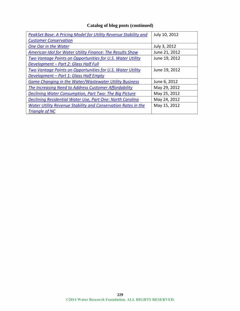
229
Catalog of blog posts (continued)
PeakSet Base: A Pricing Model for Utility Revenue Stability and Customer Conservation
July 10, 2012
One Oar in the Water July 3, 2012
American Idol for Water Utility Finance: The Results Show June 21, 2012
Two Vantage Points on Opportunities for U.S. Water Utility Development – Part 2: Glass Half Full
June 19, 2012
Two Vantage Points on Opportunities for U.S. Water Utility Development – Part 1: Glass Half Empty
June 19, 2012
Game Changing in the Water/Wastewater Utility Business June 6, 2012
The Increasing Need to Address Customer Affordability May 29, 2012
Declining Water Consumption, Part Two: The Big Picture May 25, 2012
Declining Residential Water Use, Part One: North Carolina May 24, 2012
Water Utility Revenue Stability and Conservation Rates in the Triangle of NC
May 15, 2012
©2014 Water Research Foundation. ALL RIGHTS RESERVED.


